Gaussian Processes for Machine Learning · algorithms (not just large dataset issues) Chris Williams ANC Gaussian Processes for Machine Learning. Slide from Rob Tibshirani (early

Gaussian Processes for Machine Learning

Chris Williams

Institute for Adaptive and Neural ComputationSchool of Informatics, University of Edinburgh, UK

August 2007

Chris Williams ANC


Overview

1 What is machine learning?

2 Gaussian Processes for Machine Learning

3 Multi-task Learning

Chris Williams ANC


1. What is Machine Learning?

The goal of machine learning is to build computer systemsthat can adapt and learn from their experience. (Dietterich,1999)

Machine learning usually refers to changes in systems thatperform tasks associated with artificial intelligence (AI). Suchtasks involve recognition, diagnosis, planning, robot control,prediction, etc. (Nilsson, 1996)

Some reasons for adaptation:

Some tasks can be hard to define except via examplesAdaptation can improve a human-built system, or trackchanges over time

Goals can be autonomous machine performance, or enablinghumans to learn from data (data mining)

Chris Williams ANC


Roots of Machine Learning

Statistical pattern recognition, adaptive control theory (EE)

Artificial Intelligence: e.g. discovering rules using decisiontrees, inductive logic programming

Brain models, e.g. neural networks

Psychological models

Statistics

Chris Williams ANC


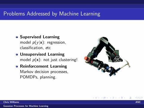
Problems Addressed by Machine Learning

Supervised Learningmodel p(y |x): regression,classification, etc

Unsupervised Learningmodel p(x): not just clustering!

Reinforcement LearningMarkov decision processes,POMDPs, planning.

Chris Williams ANC


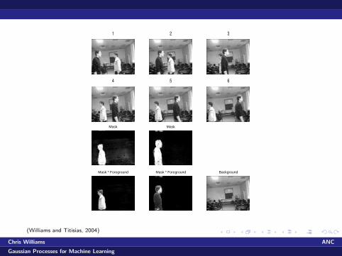
1 2 3

4 5 6

Mask

Mask * Foreground

Mask

Mask * Foreground Background

(Williams and Titisias, 2004)

Chris Williams ANC


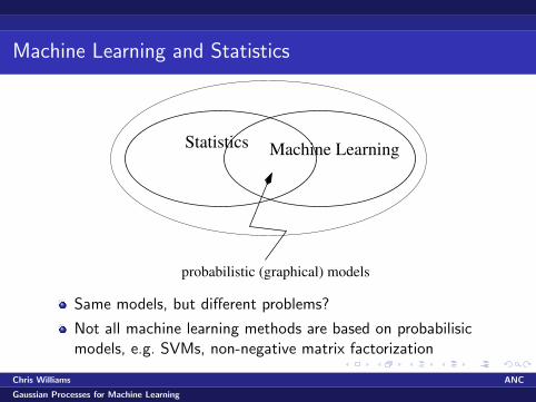
Machine Learning and Statistics

Statistics Machine Learning

probabilistic (graphical) models

Same models, but different problems?

Not all machine learning methods are based on probabilisicmodels, e.g. SVMs, non-negative matrix factorization

Chris Williams ANC


Some Differences

Statistics: focus on understanding data in terms of models

Statistics: interpretability, hypothesis testing

Machine Learning: greater focus on prediction

Machine Learning: focus on the analysis of learningalgorithms (not just large dataset issues)

Chris Williams ANC


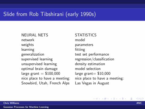
Slide from Rob Tibshirani (early 1990s)

NEURAL NETS STATISTICSnetwork modelweights parameterslearning fittinggeneralization test set performancesupervised learning regression/classificationunsupervised learning density estimationoptimal brain damage model selectionlarge grant = $100,000 large grant= $10,000nice place to have a meeting: nice place to have a meeting:Snowbird, Utah, French Alps Las Vegas in August

Chris Williams ANC


2. Gaussian Processes for Machine Learning

Gaussian processes

History

Regression, classification and beyond

Covariance functions/kernels

Dealing with hyperparameters

Theory

Approximations for large datasets

Chris Williams ANC


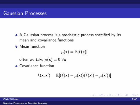
Gaussian Processes

A Gaussian process is a stochastic process specified by itsmean and covariance functions

Mean functionµ(x) = E[f (x)]

often we take µ(x) ≡ 0 ∀xCovariance function

k(x, x′) = E[(f (x)− µ(x))(f (x′)− µ(x′))]

Chris Williams ANC


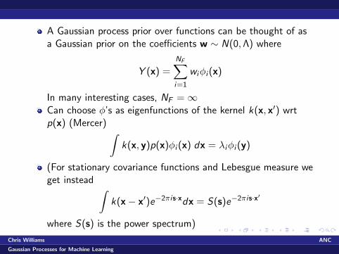
A Gaussian process prior over functions can be thought of asa Gaussian prior on the coefficients w ∼ N(0,Λ) where

Y (x) =

NF∑i=1

wiφi (x)

In many interesting cases, NF = ∞Can choose φ’s as eigenfunctions of the kernel k(x, x′) wrtp(x) (Mercer) ∫

k(x, y)p(x)φi (x) dx = λiφi (y)

(For stationary covariance functions and Lebesgue measure weget instead ∫

k(x− x′)e−2πis·xdx = S(s)e−2πis·x′

where S(s) is the power spectrum)

Chris Williams ANC


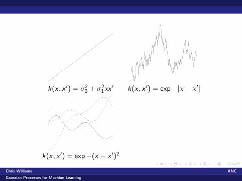
k(x , x ′) = σ20 + σ2

1xx′ k(x , x ′) = exp−|x − x ′|

k(x , x ′) = exp−(x − x ′)2

Chris Williams ANC


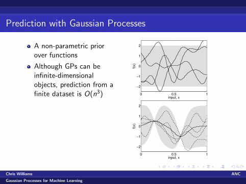
Prediction with Gaussian Processes

A non-parametric priorover functions

Although GPs can beinfinite-dimensionalobjects, prediction from afinite dataset is O(n3) 0 0.5 1

−2

−1

0

1

2

input, x

f(x)

0 0.5 1

−2

−1

0

1

2

input, x

f(x)

Chris Williams ANC


Gaussian Process Regression

Dataset D = (xi , yi )ni=1, Gaussian likelihood p(yi |fi ) ∼ N(0, σ2)

f (x) =n∑

i=1

αik(x, xi )

whereα = (K + σ2I )−1y

var(f (x)) = k(x, x)− kT (x)(K + σ2I )−1k(x)

in time O(n3), with k(x) = (k(x, x1), . . . , k(x, xn))T

Chris Williams ANC


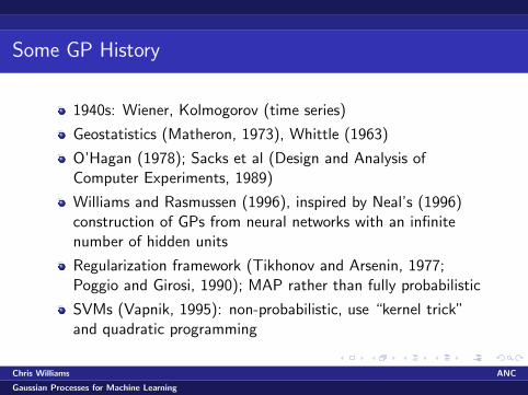
Some GP History

1940s: Wiener, Kolmogorov (time series)

Geostatistics (Matheron, 1973), Whittle (1963)

O’Hagan (1978); Sacks et al (Design and Analysis ofComputer Experiments, 1989)

Williams and Rasmussen (1996), inspired by Neal’s (1996)construction of GPs from neural networks with an infinitenumber of hidden units

Regularization framework (Tikhonov and Arsenin, 1977;Poggio and Girosi, 1990); MAP rather than fully probabilistic

SVMs (Vapnik, 1995): non-probabilistic, use “kernel trick”and quadratic programming

Chris Williams ANC


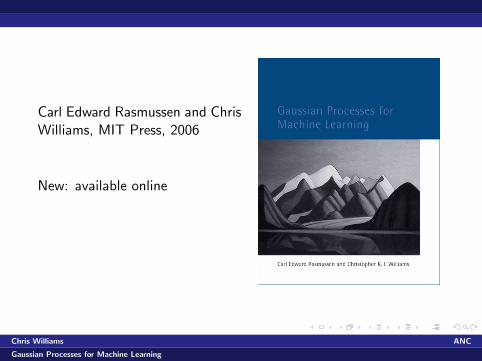
Carl Edward Rasmussen and ChrisWilliams, MIT Press, 2006

New: available online

Chris Williams ANC


Regression, classification and beyond

Regression with Gausian noise: e.g. robot arm inversedynamics (21-d input space)

Classification: binary, multiclass, e.g. handwritten digitclassification

ML community tends to use approximations to deal withnon-Gaussian likelihoods, cf MCMC in statistics?

MAP solution, Laplace approximation

Expectation Propagation (Minka, 2001; see also Opper andWinther, 2000)

Other likelihoods (e.g. Poisson), observations of derivatives,uncertain inputs, mixtures of GPs

Chris Williams ANC


Covariance functions

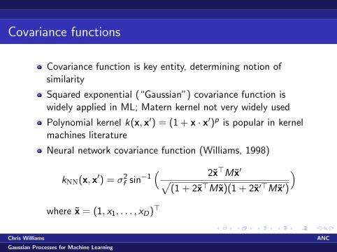
Covariance function is key entity, determining notion ofsimilarity

Squared exponential (“Gaussian”) covariance function iswidely applied in ML; Matern kernel not very widely used

Polynomial kernel k(x, x′) = (1 + x · x′)p is popular in kernelmachines literature

Neural network covariance function (Williams, 1998)

kNN(x, x′) = σ2f sin−1

( 2x>M x′√(1 + 2x>M x)(1 + 2x′>M x′)

)where x = (1, x1, . . . , xD)>

Chris Williams ANC


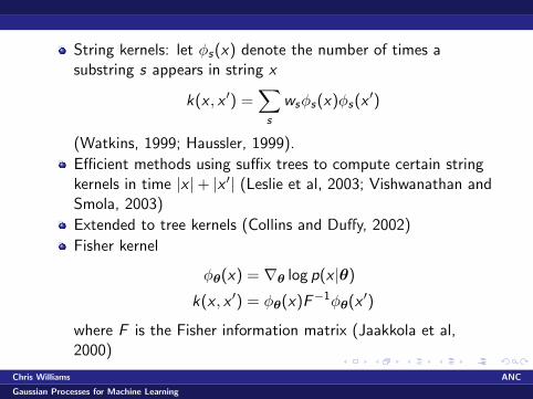
String kernels: let φs(x) denote the number of times asubstring s appears in string x

k(x , x ′) =∑

s

wsφs(x)φs(x′)

(Watkins, 1999; Haussler, 1999).

Efficient methods using suffix trees to compute certain stringkernels in time |x |+ |x ′| (Leslie et al, 2003; Vishwanathan andSmola, 2003)

Extended to tree kernels (Collins and Duffy, 2002)

Fisher kernel

φθ(x) = ∇θ log p(x |θ)

k(x , x ′) = φθ(x)F−1φθ(x ′)

where F is the Fisher information matrix (Jaakkola et al,2000)

Chris Williams ANC


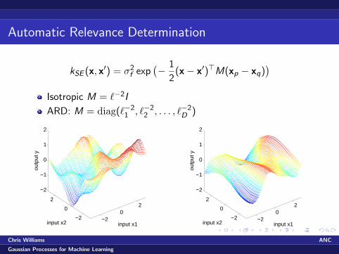
Automatic Relevance Determination

kSE (x, x′) = σ2f exp

(− 1

2(x− x′)>M(xp − xq)

)Isotropic M = `−2I

ARD: M = diag(`−21 , `−2

2 , . . . , `−2D )

−20

2

−2

0

2

−2

−1

0

1

2

input x1input x2

outp

ut y

−20

2

−2

0

2

−2

−1

0

1

2

input x1input x2

outp

ut y

Chris Williams ANC


Dealing with hyperparameters

Criteria for model selection

Marginal likelihood p(y|X ,θ)

Estimate the generalization error: LOO-CV∑ni=1 log p(yi |y−i ,X ,θ)

Bound the generalization error (e.g. PAC-Bayes)

Typically do ML-II rather than sampling of p(θ|X , y)

Optimize by gradient descent (etc) on objective function

SVMs do not generally have good methods for kernel selection

Chris Williams ANC


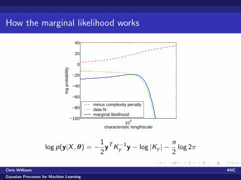
How the marginal likelihood works

100

−100

−80

−60

−40

−20

0

20

40

log

prob

abili

ty

characteristic lengthscale

minus complexity penaltydata fitmarginal likelihood

log p(y|X ,θ) = −1

2yTK−1

y y − log |Ky | −n

2log 2π

Chris Williams ANC


Marginal Likelihood and Local Optima

−5 0 5−2

−1

0

1

2

input, x

outp

ut, y

−5 0 5−2

−1

0

1

2

input, x

outp

ut, y

There can be multiple optima of the marginal likelihood

These correspond to different interpretations of the data

Chris Williams ANC


The Baby and the Bathwater

MacKay (2003 ch 45): In moving from neural networks tokernel machines did we throw out the baby with thebathwater? i.e. the ability to learn hiddenfeatures/representations

But consider M = ΛΛ> for Λ being D × k, for k < D

The k columns of Λ can identify directions in the input spacewith specially high relevance (Vivarelli and Williams, 1999)

Chris Williams ANC


Theory

Equivalent kernel (Silverman, 1984)

Consistency (Diaconis and Freedman, 1986; Choudhuri,Ghoshal and Roy 2005; Choi and Schervish, 2004)

Average case learning curves

PAC-Bayesian analysis for GPs (Seeger, 2003)

pD{RL(fD) ≤ RL(fD) + gap(fD,D, δ)} ≥ 1− δ

where RL(fD) is the expected risk, and RL(fD) is the empirical(training) risk

Chris Williams ANC


Approximation Methods for Large Datasets

Fast approximate solution of the linear system

Subset of Data

Subset of Regressors

Inducing Variables

Projected Process Approximation

FITC, PITC, BCM

SPGP

Empirical Comparison

Chris Williams ANC


Some interesting recent uses for Gaussian Processes

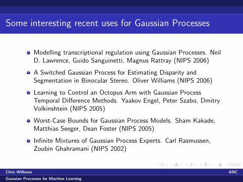
Modelling transcriptional regulation using Gaussian Processes. NeilD. Lawrence, Guido Sanguinetti, Magnus Rattray (NIPS 2006)

A Switched Gaussian Process for Estimating Disparity andSegmentation in Binocular Stereo. Oliver Williams (NIPS 2006)

Learning to Control an Octopus Arm with Gaussian ProcessTemporal Difference Methods. Yaakov Engel, Peter Szabo, DmitryVolkinshtein (NIPS 2005)

Worst-Case Bounds for Gaussian Process Models. Sham Kakade,Matthias Seeger, Dean Foster (NIPS 2005)

Infinite Mixtures of Gaussian Process Experts. Carl Rasmussen,Zoubin Ghahramani (NIPS 2002)

Chris Williams ANC


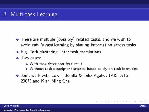
3. Multi-task Learning

There are multiple (possibly) related tasks, and we wish toavoid tabula rasa learning by sharing information across tasks

E.g. Task clustering, inter-task correlations

Two cases:

With task-descriptor features tWithout task-descriptor features, based solely on task identities

Joint work with Edwin Bonilla & Felix Agakov (AISTATS2007) and Kian Ming Chai

Chris Williams ANC


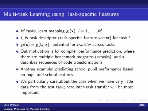
Multi-task Learning using Task-specific Features

M tasks, learn mapping gi (x), i = 1, . . . ,M

ti is task descriptor (task-specific feature vector) for task i

gi (x) = g(ti , x): potential for transfer across tasks

Out motivation is for compiler performance prediction, wherethere are multiple benchmark programs (=tasks), and xdescribes sequences of code transformations

Another example: predicting school pupil performance basedon pupil and school features

We particularly care about the case when we have very littledata from the test task; here inter-task transfer will be mostimportant

Chris Williams ANC


Overview

Model setup

Related work

Experimental setup, feature representation

Results

Discussion

Chris Williams ANC


Task-descriptor Model

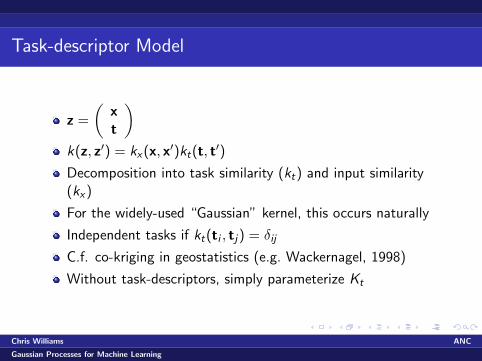
z =

(xt

)k(z, z′) = kx(x, x′)kt(t, t′)

Decomposition into task similarity (kt) and input similarity(kx)

For the widely-used “Gaussian” kernel, this occurs naturally

Independent tasks if kt(ti , tj) = δij

C.f. co-kriging in geostatistics (e.g. Wackernagel, 1998)

Without task-descriptors, simply parameterize Kt

Chris Williams ANC


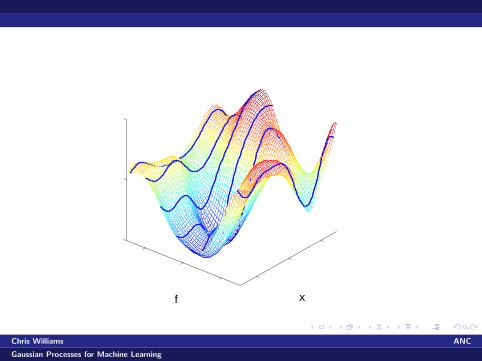
xf

Chris Williams ANC


Related Work

Work using task-specific features

Bakker and Heskes (2003) use neural networks. These can betricky to train (local optima, number of hidden units etc)

Yu et al (NIPS 2006, Stochastic Relational Models forDiscriminative Link Prediction)

Chris Williams ANC


General work on Multi-task Learning

What should be transferred?

Early work: Thrun (1996), Caruana (1997)

Minka and Picard (1999); multiple tasks share same GPhyperparameters (but are uncorrelated)

Evgeniou et al (2005): induce correlations between tasksbased on a correlated prior over linear regression parameters(special case of co-kriging)

Multilevel (or hierarchical) modelling in statistics (e.g.Goldstein, 2003)

Chris Williams ANC


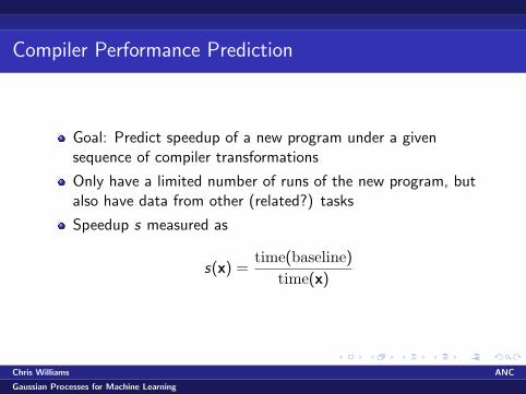
Compiler Performance Prediction

Goal: Predict speedup of a new program under a givensequence of compiler transformations

Only have a limited number of runs of the new program, butalso have data from other (related?) tasks

Speedup s measured as

s(x) =time(baseline)

time(x)

Chris Williams ANC


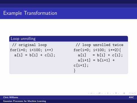
Example Transformation

Loop unrolling

// original loopfor(i=0; i<100; i++)a[i] = b[i] + c[i];

// loop unrolled twicefor(i=0; i<100; i+=2){a[i] = b[i] + c[i];a[i+1] = b[i+1] +

c[i+1];}

Chris Williams ANC


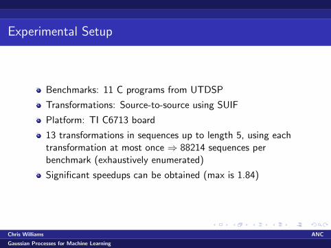
Experimental Setup

Benchmarks: 11 C programs from UTDSP

Transformations: Source-to-source using SUIF

Platform: TI C6713 board

13 transformations in sequences up to length 5, using eachtransformation at most once ⇒ 88214 sequences perbenchmark (exhaustively enumerated)

Significant speedups can be obtained (max is 1.84)

Chris Williams ANC


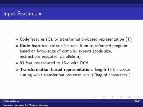
Input Features x

Code features (C), or transformation-based representation (T)

Code features: extract features from transformed programbased on knowledge of compiler experts (code size,instructions executed, parallelism)

83 features reduced to 15-d with PCA

Transformation-based representation: length-13 bit vectorstating what transformations were used (“bag of characters”)

Chris Williams ANC


Task-specific features t

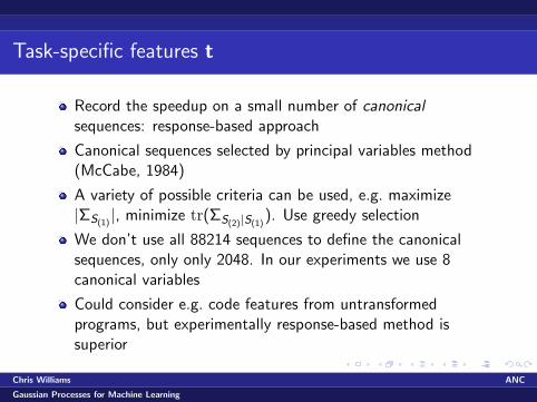
Record the speedup on a small number of canonicalsequences: response-based approach

Canonical sequences selected by principal variables method(McCabe, 1984)

A variety of possible criteria can be used, e.g. maximize|ΣS(1)

|, minimize tr(ΣS(2)|S(1)). Use greedy selection

We don’t use all 88214 sequences to define the canonicalsequences, only only 2048. In our experiments we use 8canonical variables

Could consider e.g. code features from untransformedprograms, but experimentally response-based method issuperior

Chris Williams ANC


Experiments

LOO-CV setup (leave out one task at a time)

Therefore 10 reference tasks for each prediction task; we usednr = 256 examples per benchmark

Use nte examples from the test task (nte ≥ 8)

Assess performance using mean absolute error (MAE) on allremaining test sequences

Comparison to baseline “no transfer” method using just datafrom test task

Used GP regression prediction with squared exponential kernel

ARD was used, except for “no transfer” case when nte ≤ 64

Chris Williams ANC


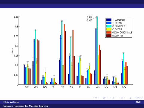
ADP COM EDG FFT FIR HIS IIR LAT LMS LPC SPE AVG0

0.05

0.1

0.15

0.2

0.25

0.3

0.35

MA

E

[T] COMBINED[T] GATING[C] COMBINED[C] GATINGMEDIAN CANONICALSMEDIAN TEST

0.540(0.007)

Chris Williams ANC


Results

T-combined is best overall (av MAE is 0.0576, compared to0.1162 for median canonicals)

T-combined generally either improves performance or leaves itabout the same compared to T-no-transfer-canonicals

Chris Williams ANC


8 16 32 64 1280

0.05

0.1

0.15

0.2

0.25

0.3

0.35

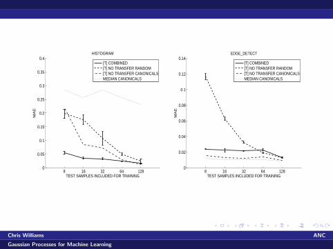
0.4HISTOGRAM

TEST SAMPLES INCLUDED FOR TRAINING

MA

E

[T] COMBINED[T] NO TRANSFER RANDOM[T] NO TRANSFER CANONICALSMEDIAN CANONICALS

8 16 32 64 1280

0.02

0.04

0.06

0.08

0.1

0.12

0.14EDGE_DETECT

TEST SAMPLES INCLUDED FOR TRAININGM

AE


Chris Williams ANC


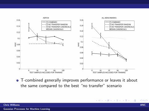
8 16 32 64 1280

0.02

0.04

0.06

0.08

0.1

0.12

0.14

0.16ADPCM


MA

E


8 16 32 64 1280

0.02

0.04

0.06

0.08

0.1

0.12

0.14

0.16

0.18


MA

E

ALL BENCHMARKS


T-combined generally improves performance or leaves it aboutthe same compared to the best “no transfer” scenario

Chris Williams ANC


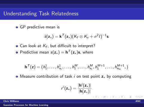
Understanding Task Relatedness

GP predictive mean is

s(z∗) = kT (z∗)(Kf ⊗ Kx + σ2I )−1s

Can look at Kf , but difficult to interpret?

Predictive mean s(z∗) = hT (z∗)s, where

hT (z) = (h11, . . . , h

1nr

, . . . , hM1 , . . . , hM

nr, hM+1

1 , . . . , hM+1nte

, )

Measure contribution of task i on test point z∗ by computing

r i (z∗) =|hi (z∗)||h(z∗)|

Chris Williams ANC


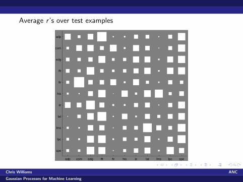
Average r ’s over test examples

adp com edg fft fir his iir lat lms lpc spe

spe

lpc

lms

lat

iir

his

fir

fft

edg

com

adp

Chris Williams ANC


Discussion

Our focus is on the hard problem of prediction on a new taskgiven very little data for that task

The presented method allows sharing over tasks. This shouldbe beneficial, but note that “no transfer” method has thefreedom to use different hyperparams on each task

Can learn similarity between tasks directly (unparameterizedKt), but this is not so easy if nte is very small

Note that there is no inter-task transfer in noiseless case!(autokrigeability)

Chris Williams ANC


General Conclusions

Key issues:

Designing/discovering covariance functions suitable for varioustypes of data

Methods for setting/inference of hyperparameters

Dealing with large datasets

Chris Williams ANC


Gaussian Process Regression

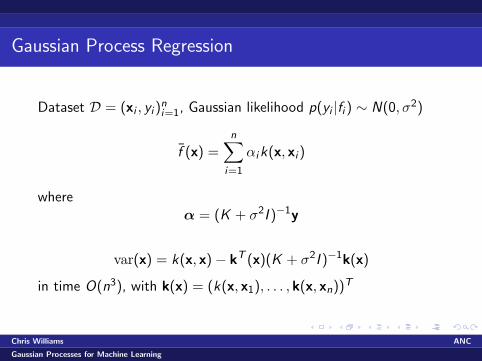
Dataset D = (xi , yi )ni=1, Gaussian likelihood p(yi |fi ) ∼ N(0, σ2)

f (x) =n∑

i=1

αik(x, xi )

whereα = (K + σ2I )−1y

var(x) = k(x, x)− kT (x)(K + σ2I )−1k(x)

in time O(n3), with k(x) = (k(x, x1), . . . , k(x, xn))T

Chris Williams ANC


Fast approximate solution of linear systems

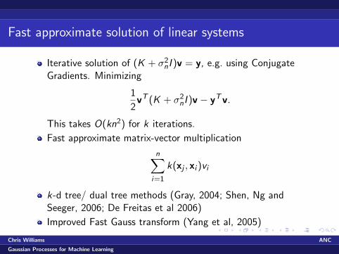
Iterative solution of (K + σ2nI )v = y, e.g. using Conjugate

Gradients. Minimizing

1

2vT (K + σ2

nI )v − yTv.

This takes O(kn2) for k iterations.

Fast approximate matrix-vector multiplication

n∑i=1

k(xj , xi )vi

k-d tree/ dual tree methods (Gray, 2004; Shen, Ng andSeeger, 2006; De Freitas et al 2006)

Improved Fast Gauss transform (Yang et al, 2005)

Chris Williams ANC


Subset of Data

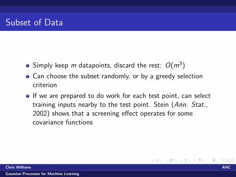
Simply keep m datapoints, discard the rest: O(m3)

Can choose the subset randomly, or by a greedy selectioncriterion

If we are prepared to do work for each test point, can selecttraining inputs nearby to the test point. Stein (Ann. Stat.,2002) shows that a screening effect operates for somecovariance functions

Chris Williams ANC


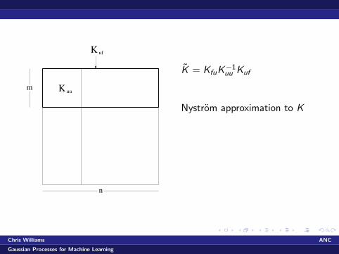
K

K

uu

uf

n

m

K = KfuK−1uu Kuf

Nystrom approximation to K

Chris Williams ANC


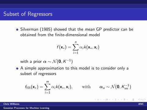
Subset of Regressors

Silverman (1985) showed that the mean GP predictor can beobtained from the finite-dimensional model

f (x∗) =n∑

i=1

αik(x∗, xi )

with a prior α ∼ N (0,K−1)

A simple approximation to this model is to consider only asubset of regressors

fSR(x∗) =m∑

i=1

αik(x∗, xi ), with αu ∼ N (0,K−1uu )

Chris Williams ANC


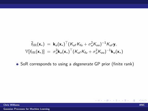
fSR(x∗) = ku(x∗)>(Kuf Kfu + σ2

nKuu)−1Kuf y,

V[fSR(x∗)] = σ2nku(x∗)

>(Kuf Kfu + σ2nKuu)

−1ku(x∗)

SoR corresponds to using a degenerate GP prior (finite rank)

Chris Williams ANC


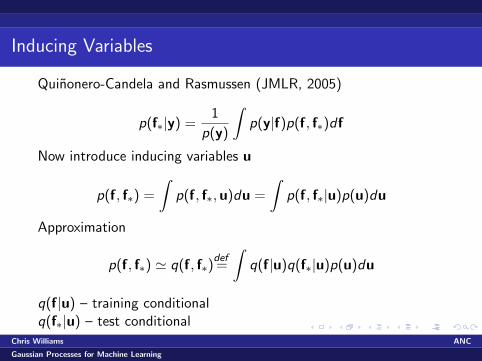
Inducing Variables

Quinonero-Candela and Rasmussen (JMLR, 2005)

p(f∗|y) =1

p(y)

∫p(y|f)p(f, f∗)df

Now introduce inducing variables u

p(f, f∗) =

∫p(f, f∗,u)du =

∫p(f, f∗|u)p(u)du

Approximation

p(f, f∗) ' q(f, f∗)def=

∫q(f|u)q(f∗|u)p(u)du

q(f|u) – training conditionalq(f∗|u) – test conditional

Chris Williams ANC


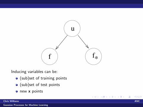
u

f f*Inducing variables can be:

(sub)set of training points

(sub)set of test points

new x points

Chris Williams ANC


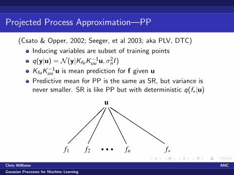
Projected Process Approximation—PP

(Csato & Opper, 2002; Seeger, et al 2003; aka PLV, DTC)

Inducing variables are subset of training points

q(y|u) = N (y|KfuK−1uu u, σ2

nI )

KfuK−1uu u is mean prediction for f given u

Predictive mean for PP is the same as SR, but variance isnever smaller. SR is like PP but with deterministic q(f∗|u)

��

��

��

��

AA

AA

AA

QQ

QQ

QQ

QQQ

u

f1 f2 r r r fn f∗

Chris Williams ANC


FITC, PITC and BCM

See Quinonero-Candela and Rasmussen (2005) for overview

Under PP, q(f|u) = N (y|KfuK−1uu u, 0)

Instead FITC (Snelson and Ghahramani, 2005) uses individualpredictive variances diag[Kff − KfuK

−1uu Kuf ], i.e. fully

independent training conditionals

PP can make poor predictions in low noise [S Q-C M R W]

PITC uses blocks of training points to improve theapproximation

BCM (Tresp, 2000) is the same approximation as PITC,except that the test points are the inducing set

Chris Williams ANC


Sparse GPs using Pseudo-inputs

(Snelson and Ghahramani, 2006)

FITC approximation, but inducing inputs are new points, inneither the training or test sets

Locations of the inducing inputs are changed along withhyperparameters so as to maximize the approximate marginallikelihood

Chris Williams ANC


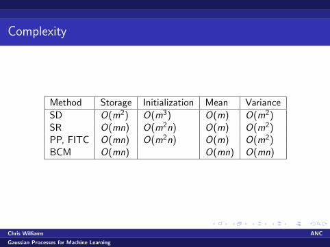
Complexity

Method Storage Initialization Mean Variance

SD O(m2) O(m3) O(m) O(m2)SR O(mn) O(m2n) O(m) O(m2)PP, FITC O(mn) O(m2n) O(m) O(m2)BCM O(mn) O(mn) O(mn)

Chris Williams ANC


Empirical Comparison

Robot arm problem, 44,484 training cases in 21-d, 4,449 testcases

For SD method subset of size m was chosen at random,hyperparameters set by optimizing marginal likelihood (ARD).Repeated 10 times

For SR, PP and BCM methods same subsets/hyperparameterswere used (BCM: hyperparameters only)

Chris Williams ANC


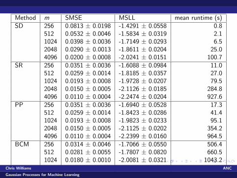
Method m SMSE MSLL mean runtime (s)SD 256 0.0813 ± 0.0198 -1.4291 ± 0.0558 0.8

512 0.0532 ± 0.0046 -1.5834 ± 0.0319 2.11024 0.0398 ± 0.0036 -1.7149 ± 0.0293 6.52048 0.0290 ± 0.0013 -1.8611 ± 0.0204 25.04096 0.0200 ± 0.0008 -2.0241 ± 0.0151 100.7

SR 256 0.0351 ± 0.0036 -1.6088 ± 0.0984 11.0512 0.0259 ± 0.0014 -1.8185 ± 0.0357 27.01024 0.0193 ± 0.0008 -1.9728 ± 0.0207 79.52048 0.0150 ± 0.0005 -2.1126 ± 0.0185 284.84096 0.0110 ± 0.0004 -2.2474 ± 0.0204 927.6

PP 256 0.0351 ± 0.0036 -1.6940 ± 0.0528 17.3512 0.0259 ± 0.0014 -1.8423 ± 0.0286 41.41024 0.0193 ± 0.0008 -1.9823 ± 0.0233 95.12048 0.0150 ± 0.0005 -2.1125 ± 0.0202 354.24096 0.0110 ± 0.0004 -2.2399 ± 0.0160 964.5

BCM 256 0.0314 ± 0.0046 -1.7066 ± 0.0550 506.4512 0.0281 ± 0.0055 -1.7807 ± 0.0820 660.51024 0.0180 ± 0.0010 -2.0081 ± 0.0321 1043.22048 0.0136 ± 0.0007 -2.1364 ± 0.0266 1920.7Chris Williams ANC


10−1 100 101 102 103 1040.01

0.02

0.03

0.04

0.05

0.06

0.07

0.08

0.09

time (s)

SMSE

SDSR and PPBCM

Chris Williams ANC


10−1 100 101 102 103 104

−2.3

−2.2

−2.1

−2

−1.9

−1.8

−1.7

−1.6

−1.5

−1.4

time (s)

MSL

LSDSRPPBCM

Chris Williams ANC


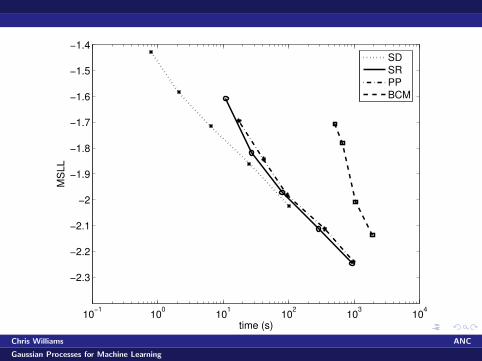
Judged on time, for this dataset SD, SR and PP are on thesame trajectory, with BCM being worse

But what about greedy vs random subset selection, methodsto set hyperparameters, different datasets?

In general, we must take into account training (initialization),testing and hyperparameter learning times separately [S Q-CM R W]. Balance will depend on your situation.

Chris Williams ANC


Documents

Gaussian Processes for Machine Learning · algorithms (not just large dataset issues) Chris Williams ANC Gaussian Processes for Machine Learning. Slide from Rob Tibshirani (early