Embed Size (px)
Citation preview
Gaussian Processes: An Introduction
Lili MOU
[email protected]://sei.pku.edu.cn/˜moull12
9 April 2015
Outline
Introduction
Kernel Tricks
Gaussian Processes for Regression
Bayesian Linear Regression
Outline
Introduction
Kernel Tricks
Gaussian Processes for Regression
Bayesian Linear Regression
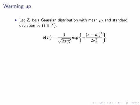
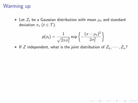
Warming up
I Let Zt be a Gaussian distribution with mean µt and standarddeviation σt (t ∈ T ).
p(zt) =1√
2πσ2t
exp
{−(x − µt)2
2σ2t
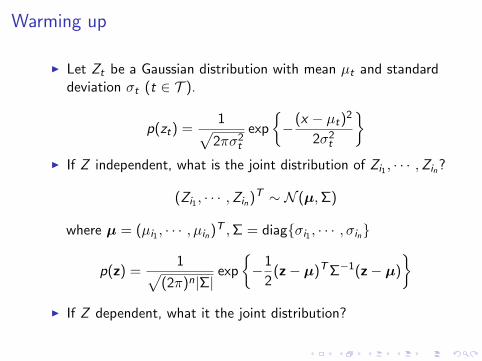
}I If Z independent, what is the joint distribution of Zi1 , · · · ,Zin?
(Zi1 , · · · ,Zin)T ∼ N (µ,Σ)
where µ = (µi1 , · · · , µin)T ,Σ = diag{σi1 , · · · , σin}
p(z) =1√
(2π)n|Σ|exp
{−1
2(z− µ)TΣ−1(z− µ)
}I If Z dependent, what it the joint distribution? Recall copulas.
Warming up
I Let Zt be a Gaussian distribution with mean µt and standarddeviation σt (t ∈ T ).
p(zt) =1√
2πσ2t
exp
{−(x − µt)2
2σ2t
}
I If Z independent, what is the joint distribution of Zi1 , · · · ,Zin?
(Zi1 , · · · ,Zin)T ∼ N (µ,Σ)
where µ = (µi1 , · · · , µin)T ,Σ = diag{σi1 , · · · , σin}
p(z) =1√
(2π)n|Σ|exp
{−1
2(z− µ)TΣ−1(z− µ)
}I If Z dependent, what it the joint distribution? Recall copulas.
Warming up
I Let Zt be a Gaussian distribution with mean µt and standarddeviation σt (t ∈ T ).
p(zt) =1√
2πσ2t
exp
{−(x − µt)2
2σ2t
}I If Z independent, what is the joint distribution of Zi1 , · · · ,Zin?
(Zi1 , · · · ,Zin)T ∼ N (µ,Σ)
where µ = (µi1 , · · · , µin)T ,Σ = diag{σi1 , · · · , σin}
p(z) =1√
(2π)n|Σ|exp
{−1
2(z− µ)TΣ−1(z− µ)
}I If Z dependent, what it the joint distribution? Recall copulas.
Warming up
I Let Zt be a Gaussian distribution with mean µt and standarddeviation σt (t ∈ T ).
p(zt) =1√
2πσ2t
exp
{−(x − µt)2
2σ2t
}I If Z independent, what is the joint distribution of Zi1 , · · · ,Zin?
(Zi1 , · · · ,Zin)T ∼ N (µ,Σ)
where µ = (µi1 , · · · , µin)T ,Σ = diag{σi1 , · · · , σin}
p(z) =1√
(2π)n|Σ|exp
{−1
2(z− µ)TΣ−1(z− µ)
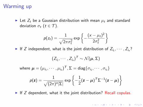
}I If Z dependent, what it the joint distribution?
Recall copulas.
Warming up
I Let Zt be a Gaussian distribution with mean µt and standarddeviation σt (t ∈ T ).
p(zt) =1√
2πσ2t
exp
{−(x − µt)2
2σ2t
}I If Z independent, what is the joint distribution of Zi1 , · · · ,Zin?
(Zi1 , · · · ,Zin)T ∼ N (µ,Σ)
where µ = (µi1 , · · · , µin)T ,Σ = diag{σi1 , · · · , σin}
p(z) =1√
(2π)n|Σ|exp
{−1
2(z− µ)TΣ−1(z− µ)
}I If Z dependent, what it the joint distribution? Recall copulas.
Stochastic Processes
Definition. A stochastic process is a set of random variables {Zt},t ∈ T . T is called an index set.
I Trivial process: Zt independent
I Brownian process
I Poisson process
The relationships between Zt are a distinguishing feature in the fieldof stochastic processes.
Gaussian Processes
Definition. A Gaussian process {Zt}, (t ∈ T ) is a stochasticprocess, each subset of {Zt} forming a (multivariate) Gaussian.
A minor question: Why not model {Zt} directly as a multivariateGaussian?
I T may have infinite elements (or even uncountable).
I What computers can deal with is finite Gaussian processes,degraded to multivariate Gaussian distributions.
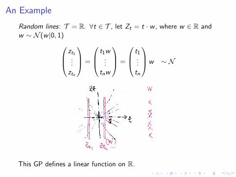
An Example
Random lines: T = R. ∀t ∈ T , let Zt = t · w , where w ∈ R andw ∼ N (w |0, 1) zt1
...ztn
=
t1w...
tnw
=
t1...tn
w ∼ N
This GP defines a linear function on R.
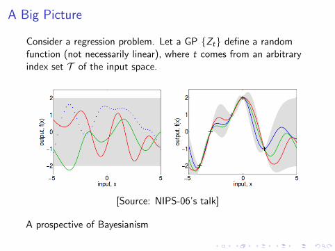
A Big Picture
Consider a regression problem. Let a GP {Zt} define a randomfunction (not necessarily linear), where t comes from an arbitraryindex set T of the input space.
[Source: NIPS-06’s talk]
A prospective of Bayesianism
Outline
Introduction
Kernel Tricks
Gaussian Processes for Regression
Bayesian Linear Regression
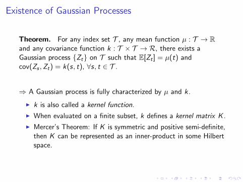
Existence of Gaussian Processes
Theorem. For any index set T , any mean function µ : T → Rand any covariance function k : T × T → R, there exists aGaussian process {Zt} on T such that E[Zt ] = µ(t) andcov(Zs ,Zt) = k(s, t), ∀s, t ∈ T .
⇒ A Gaussian process is fully characterized by µ and k.
I k is also called a kernel function.
I When evaluated on a finite subset, k defines a kernel matrix K .
I Mercer’s Theorem: If K is symmetric and positive semi-definite,then K can be represented as an inner-product in some Hilbertspace.
Random Line Revisit
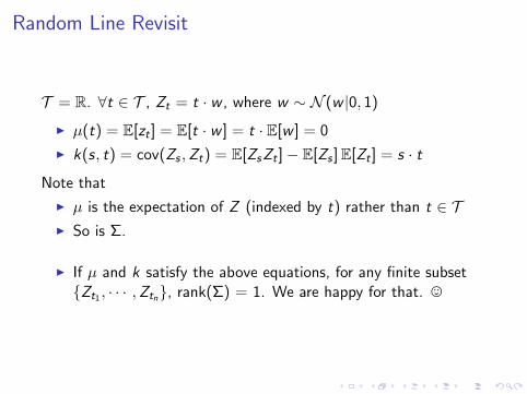
T = R. ∀t ∈ T , Zt = t · w , where w ∼ N (w |0, 1)
I µ(t) = E[zt ] = E[t · w ] = t · E[w ] = 0
I k(s, t) = cov(Zs ,Zt) = E[ZsZt ]− E[Zs ]E[Zt ] = s · t
Note that
I µ is the expectation of Z (indexed by t) rather than t ∈ TI So is Σ.
I If µ and k satisfy the above equations, for any finite subset{Zt1 , · · · ,Ztn}, rank(Σ) = 1. We are happy for that. ,
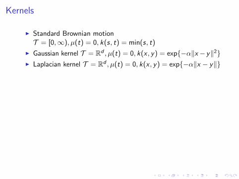
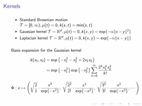
Kernels
I Standard Brownian motionT = [0,∞), µ(t) = 0, k(s, t) = min(s, t)
I Gaussian kernel T = Rd , µ(t) = 0, k(x , y) = exp{−α‖x − y‖2}I Laplacian kernel T = Rd , µ(t) = 0, k(x , y) = exp{−α‖x − y‖}
Basis expansion for the Gaussian kernel
k(x1, x2) = exp{−x2
1 − x22 + 2x1x2
}= exp
{−x2
1
}exp
{−x2
2
} ∞∑k=0
2kxk1 xk2
k!
Φ : x 7→
(√2
1· x0
exp{−x2},
√22
2!· x1
exp{−x2},
√32
3!· x2
exp{−x2}, · · ·
)
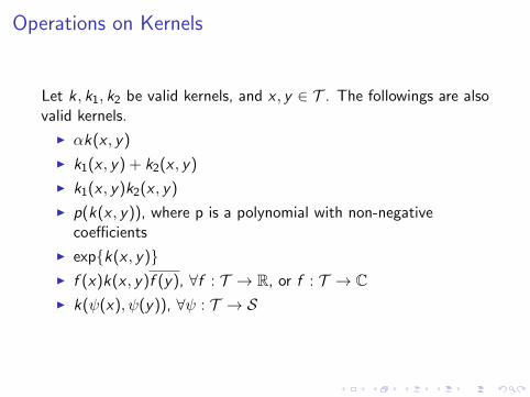
Operations on Kernels
Let k , k1, k2 be valid kernels, and x , y ∈ T . The followings are alsovalid kernels.
I αk(x , y)
I k1(x , y) + k2(x , y)
I k1(x , y)k2(x , y)
I p(k(x , y)), where p is a polynomial with non-negativecoefficients
I exp{k(x , y)}I f (x)k(x , y)f (y), ∀f : T → R, or f : T → CI k(ψ(x), ψ(y)), ∀ψ : T → S
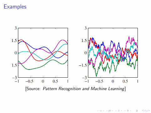
Examples
[Source: Pattern Recognition and Machine Learning ]
Generating the Random Functions
To generate the previous beautiful figures, i.e., random functionsdefined by GP(µ, k), we need to
I Take discrete points Zx1 , · · · ,Zxn in an interval
I Sample zx1 , · · · , zxn from N (µ,Σ)
I Interpolate, which is valid intuitively as long as the kernel is“smooth.”
Outline
Introduction
Kernel Tricks
Gaussian Processes for Regression
Bayesian Linear Regression
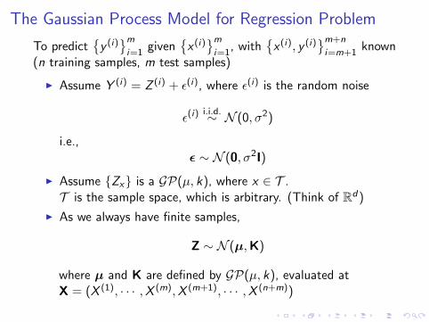
The Gaussian Process Model for Regression Problem
To predict{y (i)}mi=1
given{x (i)}mi=1
, with{x (i), y (i)
}m+n
i=m+1known
(n training samples, m test samples)
I Assume Y (i) = Z (i) + ε(i), where ε(i) is the random noise
ε(i) i.i.d.∼ N (0, σ2)
i.e.,ε ∼ N (0, σ2I)
I Assume {Zx} is a GP(µ, k), where x ∈ T .T is the sample space, which is arbitrary. (Think of Rd)
I As we always have finite samples,
Z ∼ N (µ,K)
where µ and K are defined by GP(µ, k), evaluated atX = (X (1), · · · ,X (m),X (m+1), · · · ,X (n+m))
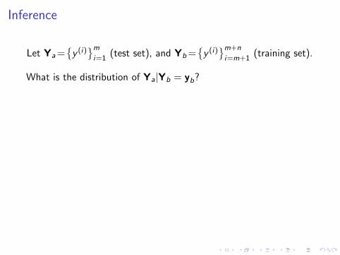
Inference
Let Ya ={y (i)}mi=1
(test set), and Yb ={y (i)}m+n
i=m+1(training set).
What is the distribution of Ya|Yb = yb?
Gaussian!
I Y = Z + ε, where Z ∼ N (µ,K) and ε ∼ N (0, σ2I)Z and ε are independent
I Y ∼ N (µ,K + σ2I)∆= N (µ,C)
I Denote Y =
(Ya
Yb
), then
µ =
(µa
µb
), and C =
(Caa Cab
Cba Cbb
)I The solution is analytic!
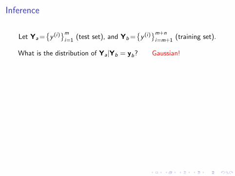
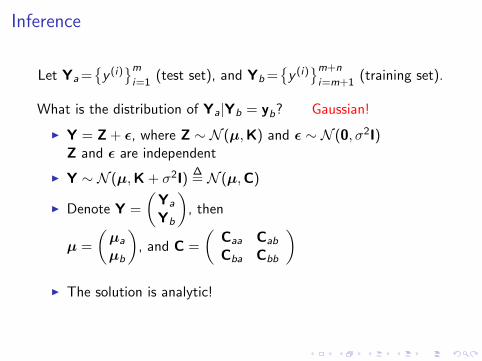
Inference
Let Ya ={y (i)}mi=1
(test set), and Yb ={y (i)}m+n
i=m+1(training set).
What is the distribution of Ya|Yb = yb? Gaussian!
I Y = Z + ε, where Z ∼ N (µ,K) and ε ∼ N (0, σ2I)Z and ε are independent
I Y ∼ N (µ,K + σ2I)∆= N (µ,C)
I Denote Y =
(Ya
Yb
), then
µ =
(µa
µb
), and C =
(Caa Cab
Cba Cbb
)I The solution is analytic!
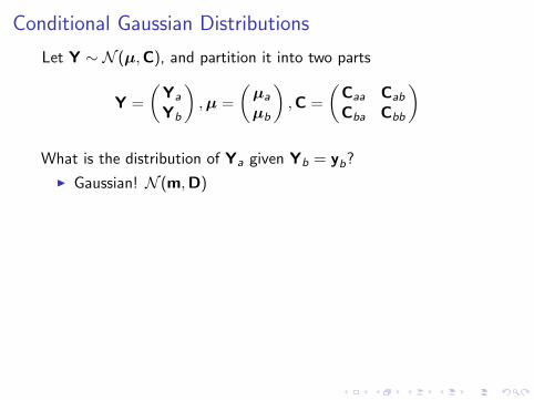
Conditional Gaussian Distributions
Let Y ∼ N (µ,C), and partition it into two parts
Y =
(Ya
Yb
),µ =
(µa
µb
),C =
(Caa Cab
Cba Cbb
)
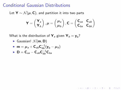
What is the distribution of Ya given Yb = yb?
I Gaussian! N (m,D)
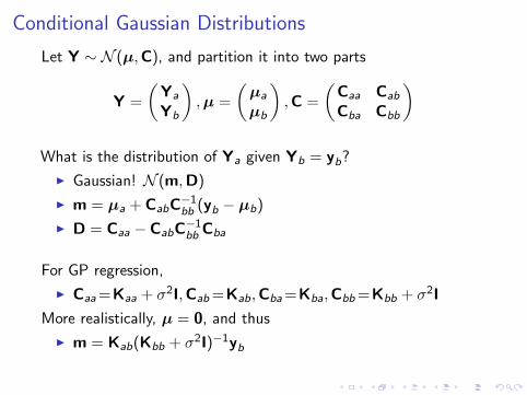
I m = µa + CabC−1bb (yb − µb)
I D = Caa − CabC−1bb Cba
For GP regression,
I Caa =Kaa + σ2I,Cab =Kab,Cba =Kba,Cbb =Kbb + σ2I
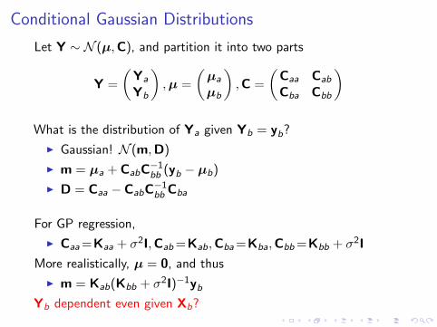
More realistically, µ = 0, and thus
I m = Kab(Kbb + σ2I)−1ybYb dependent even given Xb?
Conditional Gaussian Distributions
Let Y ∼ N (µ,C), and partition it into two parts
Y =
(Ya
Yb
),µ =
(µa
µb
),C =
(Caa Cab
Cba Cbb
)
What is the distribution of Ya given Yb = yb?
I Gaussian! N (m,D)
I m = µa + CabC−1bb (yb − µb)
I D = Caa − CabC−1bb Cba
For GP regression,
I Caa =Kaa + σ2I,Cab =Kab,Cba =Kba,Cbb =Kbb + σ2I
More realistically, µ = 0, and thus
I m = Kab(Kbb + σ2I)−1yb
Yb dependent even given Xb?
Conditional Gaussian Distributions
Let Y ∼ N (µ,C), and partition it into two parts
Y =
(Ya
Yb
),µ =
(µa
µb
),C =
(Caa Cab
Cba Cbb
)
What is the distribution of Ya given Yb = yb?
I Gaussian! N (m,D)
I m = µa + CabC−1bb (yb − µb)
I D = Caa − CabC−1bb Cba
For GP regression,
I Caa =Kaa + σ2I,Cab =Kab,Cba =Kba,Cbb =Kbb + σ2I
More realistically, µ = 0, and thus
I m = Kab(Kbb + σ2I)−1ybYb dependent even given Xb?
Outline
Introduction
Kernel Tricks
Gaussian Processes for Regression
Bayesian Linear Regression
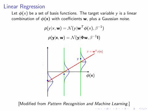
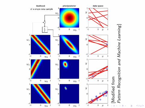
Linear RegressionLet φ(x) be a set of basis functions. The target variable y is a linearcombination of φ(x) with coefficients w, plus a Gaussian noise.
p(y |x ,w) = N (y |wTφ(x), β−1)
p(y|x,w) = N (y|Φw, β−1I)
[Modified from Pattern Recognition and Machine Learning.]
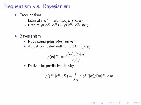
Frequentism v.s. Bayesianism
I Frequentism
- Estimate w∗ = argmaxw p(y|x; w)- Predict p̂(y (t)|x (t)) = p(y (t)|x (t); w∗)
I BayesianismI Have some prior p(w) on wI Adjust our belief with data D = {x, y}
p(w|D) =p(w)p(D|w)
p(D)
I Derive the predictive density
p(y (t)|x (t),D) =
∫W
p(y (t)|w)p(w|D) d w
Note that
I Mathematicians are happy , if prior and posterior distributionstake the same form. (Called conjugate priors.)
I Most problems do not have closed-form solutions.
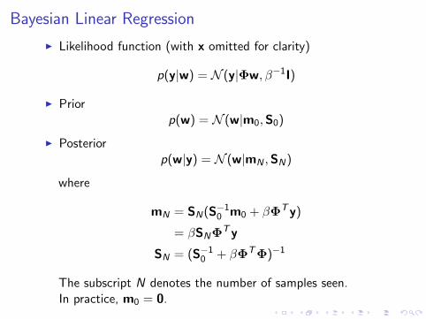
Bayesian Linear Regression
I Likelihood function (with x omitted for clarity)
p(y|w) = N (y|Φw, β−1I)
I Priorp(w) = N (w|m0,S0)
I Posteriorp(w|y) = N (w|mN ,SN)
where
mN = SN(S−10 m0 + βΦTy)
= βSNΦTy
SN = (S−10 + βΦTΦ)−1
The subscript N denotes the number of samples seen.In practice, m0 = 0.
[Mo
difi
edfr
om
Pattern
Recog
nitionandMachineLearning
]
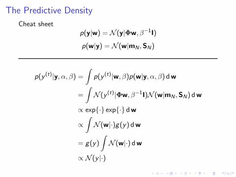
The Predictive Density
Cheat sheetp(y|w) = N (y|Φw, β−1I)
p(w|y) = N (w|mN ,SN)
p(y (t)|y, α, β) =
∫p(y (t)|w, β)p(w|y, α, β) d w
=
∫N (y (t)|Φw, β−1I)N (w|mN ,SN) d w
∝ exp{·} exp{·} d w
∝∫N (w|·)g(y) d w
= g(y)
∫N (w|·) d w
∝ N (y |·)
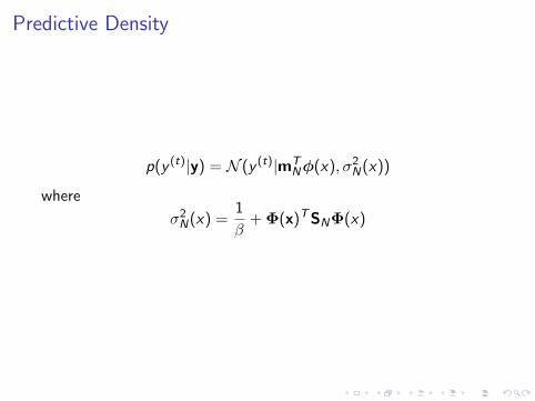
Predictive Density
p(y (t)|y) = N (y (t)|mTNφ(x), σ2
N(x))
where
σ2N(x) =
1
β+ Φ(x)TSNΦ(x)
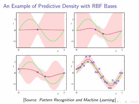
An Example of Predictive Density with RBF Bases
[Source: Pattern Recognition and Machine Learning ]
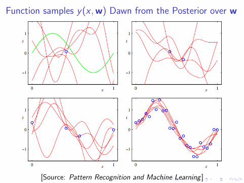
Function samples y(x ,w) Dawn from the Posterior over w
[Source: Pattern Recognition and Machine Learning ]
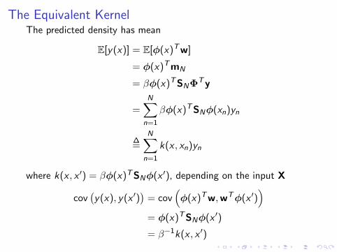
The Equivalent KernelThe predicted density has mean
E[y(x)] = E[φ(x)Tw]
= φ(x)TmN
= βφ(x)TSNΦTy
=N∑
n=1
βφ(x)TSNφ(xn)yn
∆=
N∑n=1
k(x , xn)yn
where k(x , x ′) = βφ(x)TSNφ(x ′), depending on the input X
cov(y(x), y(x ′)
)= cov
(φ(x)Tw,wTφ(x ′)
)= φ(x)TSNφ(x ′)
= β−1k(x , x ′)
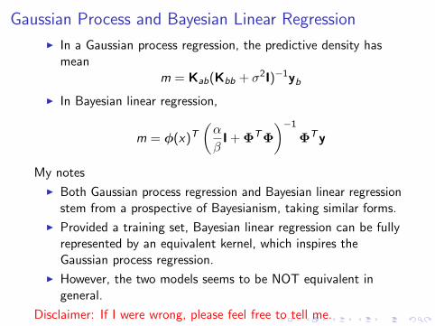
Gaussian Process and Bayesian Linear Regression
I In a Gaussian process regression, the predictive density hasmean
m = Kab(Kbb + σ2I)−1yb
I In Bayesian linear regression,
m = φ(x)T(α
βI + ΦTΦ
)−1
ΦTy
My notes
I Both Gaussian process regression and Bayesian linear regressionstem from a prospective of Bayesianism, taking similar forms.
I Provided a training set, Bayesian linear regression can be fullyrepresented by an equivalent kernel, which inspires theGaussian process regression.
I However, the two models seems to be NOT equivalent ingeneral.
Disclaimer: If I were wrong, please feel free to tell me.
References
I Pattern Recognition and Machine Learning
I Machine Learning: A Probabilistic Prospective
I http://www.gaussianprocess.org/
I https://www.youtube.com/user/mathematicalmonk