Embed Size (px)
DESCRIPTION
Gauss Quadrature Rule of Integration. Electrical Engineering Majors Authors: Autar Kaw, Charlie Barker http://numericalmethods.eng.usf.edu Transforming Numerical Methods Education for STEM Undergraduates. Gauss Quadrature Rule of Integration http://numericalmethods.eng.usf.edu. f(x). y. a. - PowerPoint PPT Presentation
Citation preview
04/20/23http://
numericalmethods.eng.usf.edu 1
Gauss Quadrature Rule of Integration
Electrical Engineering Majors
Authors: Autar Kaw, Charlie Barker
http://numericalmethods.eng.usf.eduTransforming Numerical Methods Education for STEM
Undergraduates
Gauss Quadrature Rule of Integration
http://numericalmethods.eng.usf.edu
http://numericalmethods.eng.usf.edu3
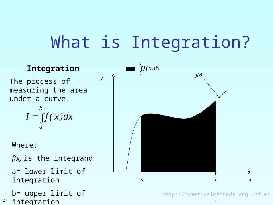
What is Integration?Integration
b
a
dx)x(fI
The process of measuring the area under a curve.
Where:
f(x) is the integrand
a= lower limit of integration
b= upper limit of integration
f(x)
a b
y
x
b
a
dx)x(f
http://numericalmethods.eng.usf.edu4
Two-Point Gaussian Quadrature Rule
http://numericalmethods.eng.usf.edu5
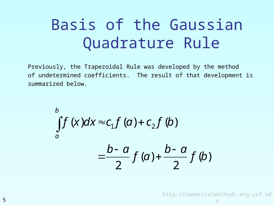
Basis of the Gaussian Quadrature Rule
Previously, the Trapezoidal Rule was developed by the methodof undetermined coefficients. The result of that development issummarized below.
)(2
)(2
)()()( 21
bfab
afab
bfcafcdxxfb
a
http://numericalmethods.eng.usf.edu6
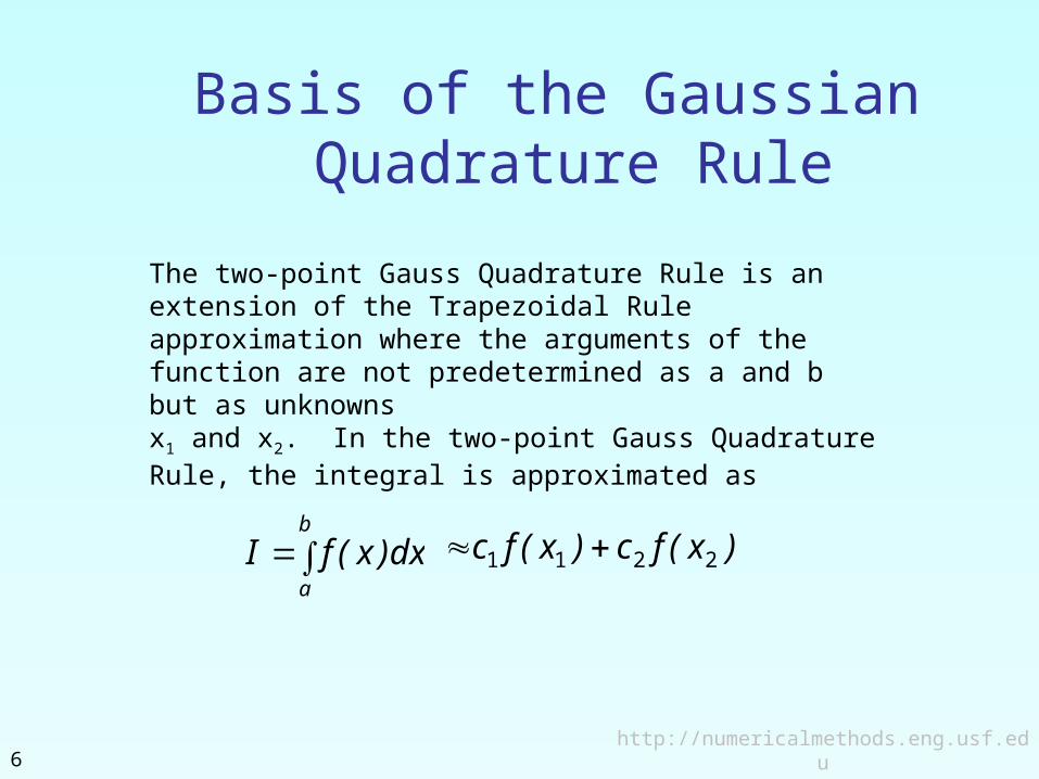
Basis of the Gaussian Quadrature Rule
The two-point Gauss Quadrature Rule is an extension of the Trapezoidal Rule approximation where the arguments of the function are not predetermined as a and b but as unknownsx1 and x2. In the two-point Gauss Quadrature Rule, the integral is approximated as
b
a
dx)x(fI )x(fc)x(fc 2211
http://numericalmethods.eng.usf.edu7
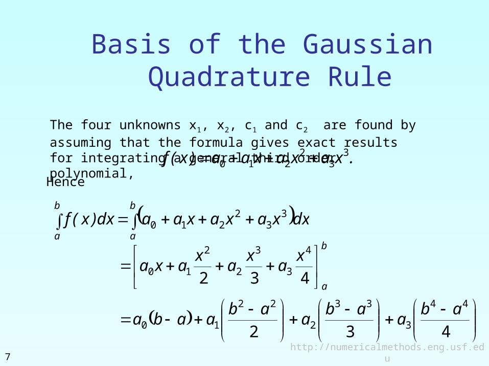
Basis of the Gaussian Quadrature Rule
The four unknowns x1, x2, c1 and c2 are found by assuming that the formula gives exact results for integrating a general third order polynomial, .xaxaxaa)x(f 3
32
210 Hence
b
a
b
a
dxxaxaxaadx)x(f 33
2210
b
a
xa
xa
xaxa
432
4
3
3
2
2
10
432
44
3
33
2
22
10
aba
aba
abaaba
http://numericalmethods.eng.usf.edu8
Basis of the Gaussian Quadrature Rule
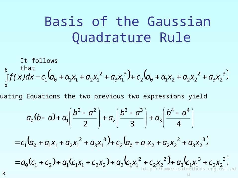
It follows that
323
2222102
313
2121101 xaxaxaacxaxaxaacdx)x(f
b
a
Equating Equations the two previous two expressions yield
432
44
3
33
2
22
10
aba
aba
abaaba
323
2222102
313
2121101 xaxaxaacxaxaxaac
322
3113
222
211222111210 xcxcaxcxcaxcxcacca
http://numericalmethods.eng.usf.edu9
Basis of the Gaussian Quadrature Rule
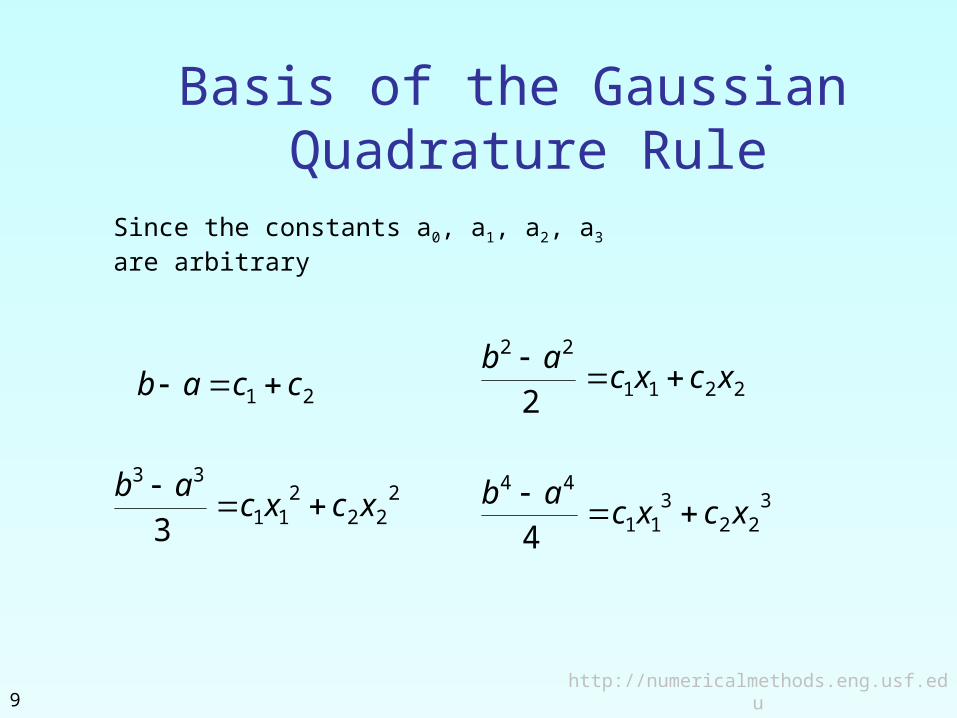
Since the constants a0, a1, a2, a3 are arbitrary
21 ccab 2211
22
2xcxc
ab
222
211
33
3xcxc
ab
3
223
11
44
4xcxc
ab
http://numericalmethods.eng.usf.edu10
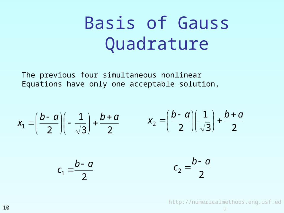
Basis of Gauss Quadrature
The previous four simultaneous nonlinear Equations have only one acceptable solution,
21
abc
22
abc
23
1
21
ababx
23
1
22
ababx
http://numericalmethods.eng.usf.edu11
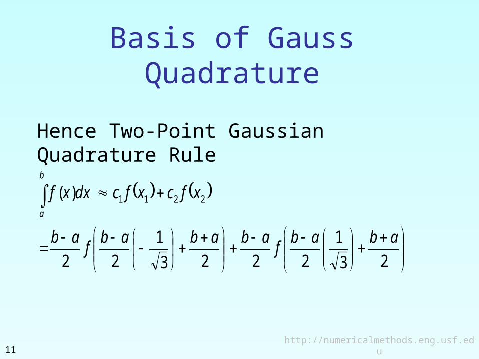
Basis of Gauss Quadrature
Hence Two-Point Gaussian Quadrature Rule
23
1
2223
1
22
)( 2211
ababf
abababf
ab
xfcxfcdxxfb
a
http://numericalmethods.eng.usf.edu12
Higher Point Gaussian Quadrature Formulas
http://numericalmethods.eng.usf.edu13
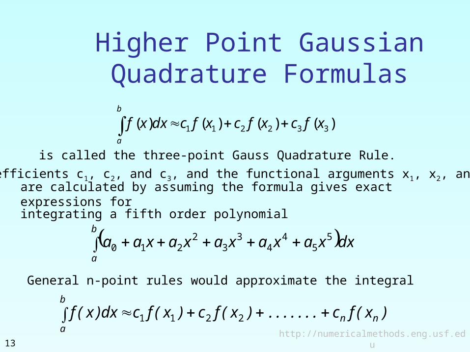
Higher Point Gaussian Quadrature Formulas
)()()()( 332211 xfcxfcxfcdxxfb
a
is called the three-point Gauss Quadrature Rule.
The coefficients c1, c2, and c3, and the functional arguments x1, x2, and x3
are calculated by assuming the formula gives exact expressions for
b
a
dxxaxaxaxaxaa 55
44
33
2210
General n-point rules would approximate the integral
)x(fc.......)x(fc)x(fcdx)x(f nn
b
a
2211
integrating a fifth order polynomial
http://numericalmethods.eng.usf.edu14
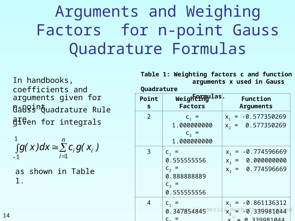
Arguments and Weighing Factors for n-point Gauss
Quadrature Formulas
In handbooks, coefficients and
Gauss Quadrature Rule are
1
1 1
n
iii )x(gcdx)x(g
as shown in Table 1.
Points
WeightingFactors
FunctionArguments
2 c1 = 1.000000000
c2 = 1.000000000
x1 = -0.577350269x2 = 0.577350269
3 c1 = 0.555555556c2 = 0.888888889c3 = 0.555555556
x1 = -0.774596669x2 = 0.000000000x3 = 0.774596669
4 c1 = 0.347854845c2 = 0.652145155c3 = 0.652145155c4 = 0.347854845
x1 = -0.861136312x2 = -0.339981044x3 = 0.339981044x4 = 0.861136312
arguments given for n-point
given for integrals
Table 1: Weighting factors c and function arguments x used in Gauss Quadrature Formulas.
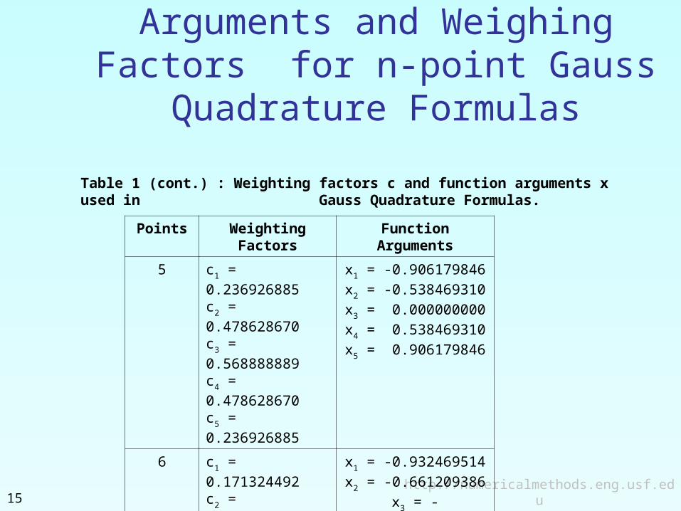
http://numericalmethods.eng.usf.edu15
Arguments and Weighing Factors for n-point Gauss
Quadrature Formulas
Points WeightingFactors
FunctionArguments
5 c1 = 0.236926885c2 = 0.478628670c3 = 0.568888889c4 = 0.478628670c5 = 0.236926885
x1 = -0.906179846x2 = -0.538469310x3 = 0.000000000x4 = 0.538469310x5 = 0.906179846
6 c1 = 0.171324492c2 = 0.360761573c3 = 0.467913935c4 = 0.467913935c5 = 0.360761573c6 = 0.171324492
x1 = -0.932469514x2 = -0.661209386
x3 = -0.2386191860
x4 = 0.2386191860x5 = 0.661209386x6 = 0.932469514
Table 1 (cont.) : Weighting factors c and function arguments x used in Gauss Quadrature Formulas.
http://numericalmethods.eng.usf.edu16
Arguments and Weighing Factors for n-point Gauss
Quadrature Formulas
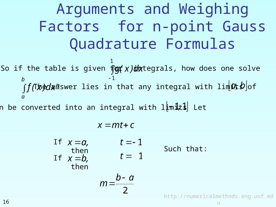
So if the table is given for
1
1
dx)x(g integrals, how does one solve
b
a
dx)x(f ? The answer lies in that any integral with limits of b,a
can be converted into an integral with limits 11, Let
cmtx
If then,ax 1t
,bx If then 1tSuch that:
2
abm
http://numericalmethods.eng.usf.edu17
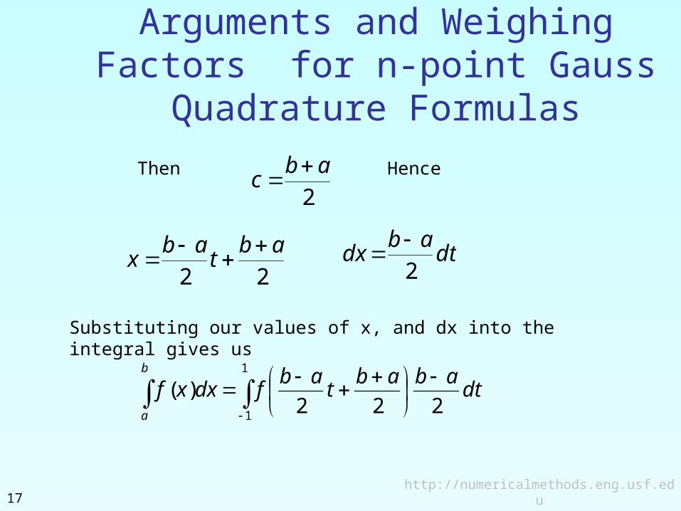
Arguments and Weighing Factors for n-point Gauss
Quadrature Formulas
2
abc
Then Hence
22
abtab
x
dtab
dx2
Substituting our values of x, and dx into the integral gives us
1
1 222)( dt
ababtab
fdxxfb
a
http://numericalmethods.eng.usf.edu18
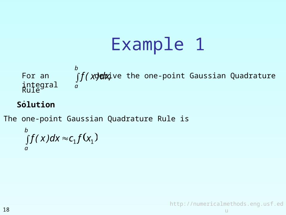
Example 1
For an integral
derive the one-point Gaussian Quadrature
Rule.
,dx)x(fb
a
Solution
The one-point Gaussian Quadrature Rule is
11 xfcdx)x(fb
a
http://numericalmethods.eng.usf.edu19
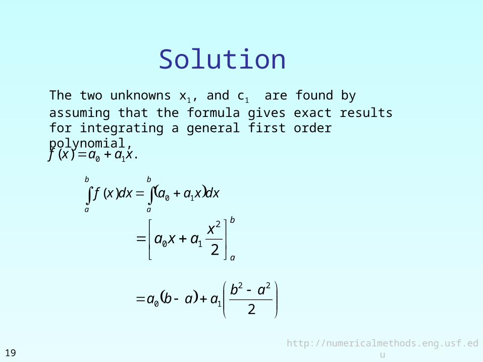
SolutionThe two unknowns x1, and c1 are found by assuming that the formula gives exact results for integrating a general first order polynomial,
.)( 10 xaaxf
b
a
b
a
dxxaadxxf 10)(
b
a
xaxa
2
2
10
2
22
10
abaaba
http://numericalmethods.eng.usf.edu20
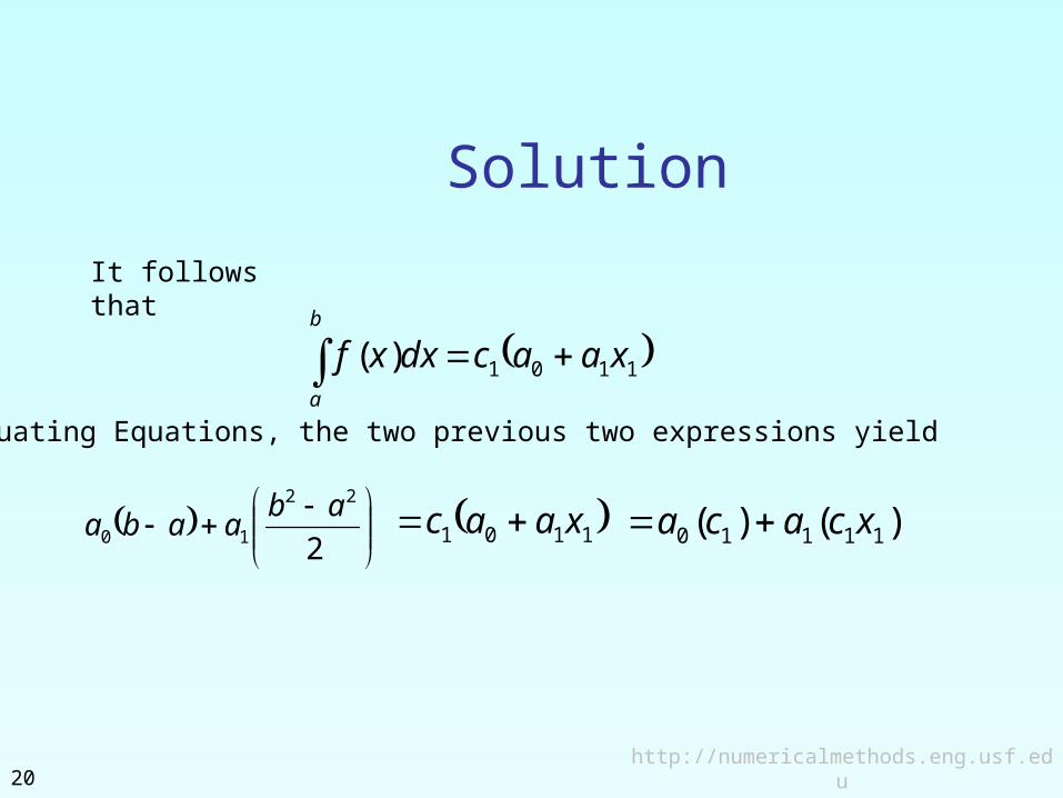
Solution
It follows that
1101)( xaacdxxfb
a
Equating Equations, the two previous two expressions yield
2
22
10
abaaba 1101 xaac )()( 11110 xcaca
http://numericalmethods.eng.usf.edu21
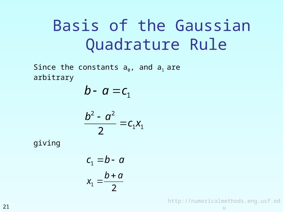
Basis of the Gaussian Quadrature Rule
Since the constants a0, and a1 are arbitrary
1cab
11
22
2xc
ab
abc 1
21
abx
giving
http://numericalmethods.eng.usf.edu22
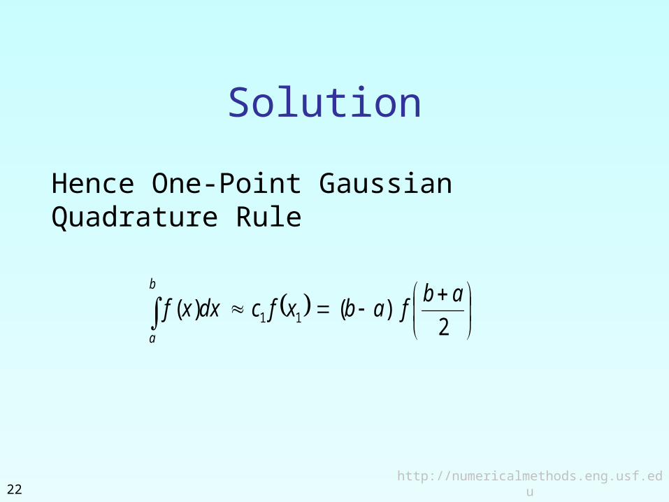
Solution
Hence One-Point Gaussian Quadrature Rule
2)()( 11
abfabxfcdxxf
b
a
http://numericalmethods.eng.usf.edu23
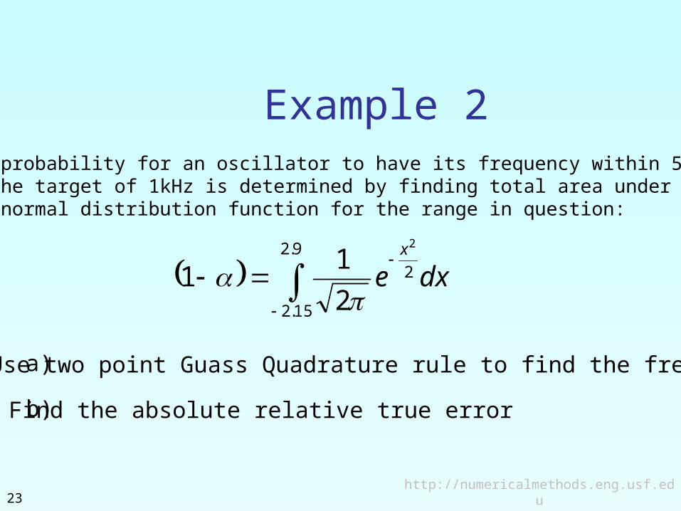
Example 2
a)
b)
The probability for an oscillator to have its frequency within 5%of the target of 1kHz is determined by finding total area underthe normal distribution function for the range in question:
Use two point Guass Quadrature rule to find the frequency
Find the absolute relative true error
9.2
15.2
2
2
2
11 dxe
x
http://numericalmethods.eng.usf.edu24
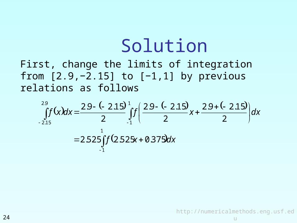
SolutionFirst, change the limits of integration from [2.9,−2.15] to [−1,1] by previous relations as follows
1
1
1
1
9.2
15.2
375.0525.2525.2
2
15.29.2
2
15.29.2
2
15.29.2
dxxf
dxxfdxxf
http://numericalmethods.eng.usf.edu25
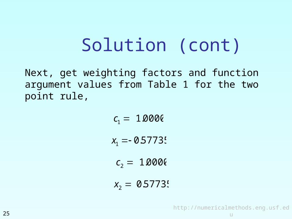
Solution (cont)Next, get weighting factors and function argument values from Table 1 for the two point rule,
0000.11 c
57735.01 x
0000.12 c
57735.02 x
http://numericalmethods.eng.usf.edu26
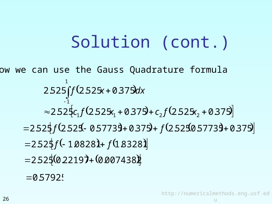
Solution (cont.)
Now we can use the Gauss Quadrature formula
57925.0
375.0525.2375.0525.2525.2
375.0525.2525.2
2211
1
1
xfcxfc
dxxf
375.057735.0525.2375.057735.0525.2525.2 ff
83281.108281.1525.2 ff
0074382.022197.0525.2
http://numericalmethods.eng.usf.edu27
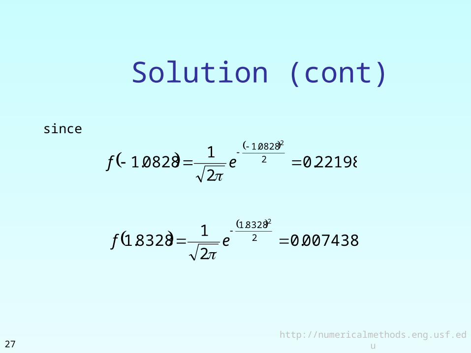
Solution (cont)
since
22198.02
10828.1 2
0828.1 2
ef
0074383.02
18328.1 2
8328.1 2
ef
http://numericalmethods.eng.usf.edu28
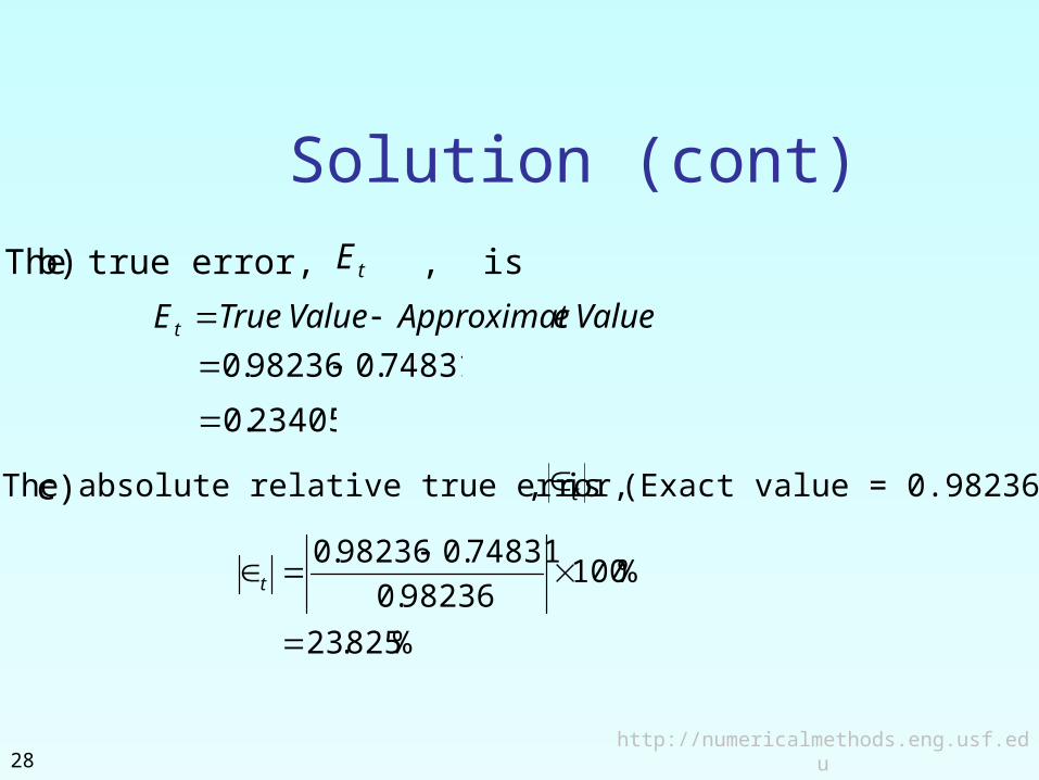
Solution (cont)
The absolute relative true error, t, is (Exact value = 0.98236)
%825.23
%10098236.0
74831.098236.0
t
c)
The true error, , isb) tE
ValueeApproximatValueTrueEt 74831.098236.0 23405.0
Additional ResourcesFor all resources on this topic such as digital audiovisual lectures, primers, textbook chapters, multiple-choice tests, worksheets in MATLAB, MATHEMATICA, MathCad and MAPLE, blogs, related physical problems, please visit
http://numericalmethods.eng.usf.edu/topics/gauss_quadrature.html
![Gene H. Golubnasonline.org/publications/biographical-memoirs/... · Kronrod [CGGR00], Gauss-Radau and Gauss-Lobatto quadrature [Gol73]. Other authors have generalized further. The](https://img.pdfslide.us/doc/110x75/5f485b28dc757434613d5adb/gene-h-kronrod-cggr00-gauss-radau-and-gauss-lobatto-quadrature-gol73-other.jpg)