Embed Size (px)
Citation preview

Valuing Credit Derivatives Using Gaussian Quadrature :
A Stochastic Volatility Framework
Nabil TAHANI *
(First version: June 2002 ; This version: January 2003)
Contact information
Nabil Tahani
HEC Montréal
Department of Finance, Office 4-455
3000, Chemin de la Côte-Sainte-Catherine
Montreal (Quebec)
Canada H3T 2A7
Phone : 1 (514) 340-7158
Fax : 1 (514) 340-5019
E-mail : [email protected]

Valuing Credit Derivatives Using Gaussian Quadrature :
A Stochastic Volatility Framework
Abstract
This paper proposes semi-closed-form solutions to value derivatives on mean-reverting
assets. We consider a very general mean-reverting process for the underlying asset and two
stochastic volatility processes: the Square-Root process and the Ornstein-Uhlenbeck
process. For both models, we derive semi-closed-form solutions for Characteristic
Functions, in which we need to solve simple Ordinary Differential Equations, and then
invert them to recover the cumulative probabilities using the Gaussian-Laguerre quadrature
rule. As benchmarks, we use our models to value European Call options within Black-
Scholes (1973) (represents constant volatility and no mean-reversion), Longstaff-Schwartz
(1995) (represents constant volatility and mean-reversion), Heston (1993) and Zhu (2000)
(represent stochastic volatility and no mean-reversion) frameworks. These comparisons
show that we only need polynomials with small degree for convergence and accuracy.
Indeed, when applied to our processes (represent stochastic volatility and mean-reversion),
the Gaussian-Laguerre rule is very efficient and very accurate. We also show that the mean-
reversion could have a large impact on option prices even though the strength of the
reversion is small. As applications, we value credit spread options, caps, floors and swaps.
Keywords : Mean-reversion, Stochastic Volatility, Gaussian Quadrature, Inverse Fourier
Transform, Feynman-Kac Theorem, Credit Spread Options, Caps, Floors, Swaps.
JEL Classification : G13, C63

2
Some assets such as interest rates, credit spreads and some commodities are shown to
exhibit mean-reversion feature. Many papers price derivatives on these assets under constant
volatility assumption. Cox, Ingersoll and Ross (1985) propose a general equilibrium model
and derive a square-root interest rate model and the discount bond pricing formula as well as
the bond option price. Longstaff and Schwartz (1995) show that the log-credit spreads are
mean-reverting. Assuming that they could be modelled with a Gaussian process, they derive
a simple closed-form solution for European options. Schwartz (1997) proposes a mean-
reverting process for commodities in order to price some derivatives. But all these models
have the common point that the volatility is assumed non-stochastic, which is a strong
simplification that omits some empirical features like leptokurtic distributions and leads to
unrealistic option prices.
In this way, substantial progress has been made in developing more realistic option
pricing models by incorporating stochastic volatility and jumps. Heston (1993) prices
European options on stocks, bonds and currencies under a square-root volatility process. In
the same way, Bakshi, Cao and Chen (1997) combine stochastic volatility and jumps to test
the empirical performance of some alternative option pricing models. Schöbel and Zhu
(1998) and Zhu (2000) propose a more elegant method to derive option prices under some
volatility models such as the square-root and the Ornstein-Uhlenbeck. While all these papers
propose simple and easy-to-use closed-form solutions to non-mean-reverting assets
derivatives under stochastic volatility assumption, there is a little literature for mean-
reverting assets within stochastic volatility frameworks.
Assuming a square-root volatility and Vasicek’s (1977) interest rate process, Fong
and Vasicek (1992) develop the fundamental partial differential equation for interest rate
contingent claims but derive a closed-form solution only for discount bonds. This solution
3
requires a heavy computation of the confluent hypergeometric function within the complex
numbers algebra. To override this difficulty, Selby and Strickland (1995) propose a series
solution for the discount bond price that is very efficient. In another paper (1997), they also
develop a Monte Carlo valuation of other interest rate derivatives under the Fong and
Vasicek (1992) model. In a discrete-time framework, Tahani (2000) proposes a closed-form
valuation formula for credit spread options under GARCH as a generalization of Longstaff
and Schwartz (1995) and Heston and Nandi (2000) models. He also shows that the GARCH
used has the square-root mean-reverting process, one of the two models used in the current
paper, as a continuous-time limit.
In this paper, we propose to derive pricing formulas for options on mean-reverting
assets within two stochastic volatility frameworks, the square-root and the Ornstein-
Uhlenbeck processes. In this, we generalize the Longstaff and Schwartz (1995) constant
volatility model and the work done by Heston (1993) and Zhu (2000) by incorporating a
mean-reverting component. Our work also extends the Fong and Vasicek (1992) model
since we propose a semi-analytic valuation framework for some derivatives on general
mean-reverting assets instead of using Monte Carlo simulation as done by Selby and
Strickland (1997). Monte Carlo methods may need a large number of paths simulation
which makes semi-analytic valuation, when possible, much more efficient.
For both stochastic volatility models considered in this paper, we derive semi-closed-
form characteristic functions in which we only need to solve simple ordinary differential
equations (ODEs). In the square-root case, even though we derive complete closed-form
solution (it involves the Whittaker functions that are related to the confluent hypergeometric
function), we show that a numerical resolution of the ODEs provides us with as accurate
values as the exact ones but in much less time. This is due to the fact that when one deals
4
with complex functions that could only be computed approximately as a series expansion
(like Whittaker and the confluent hypergeometric functions) even with some mathematical
softwares such as Maple® or Mathematica®, one has to face large time computation and
usually overflow errors.
Once the characteristic function derived in a semi-closed-form way, we use the
inverse Fourier transform technique to get the associated cumulative probabilities by a
numerical integration based on the Gauss-Laguerre quadrature rule. The Gaussian
integration technique was proved very efficient and accurate in many papers among which
Bates (1996), who prices currency options within a stochastic volatility and jumps
framework, and Sullivan (2000) who proposes an approximation to American Put options.
In our frameworks, using some benchmark such as the Black and Scholes (1973), the
Longstaff and Schwartz (1995), the Heston (1993) and the Zhu (2000) models, the Gauss-
Laguerre quadrature rule is shown to be very accurate and convergent to the true price even
with small polynomial degree. As applications, we value credit spread options, caps, floors
and swaps.
The contribution of this work is twofold. We propose a semi-analytic procedure to
price derivatives on very general mean-reverting underlying assets under stochastic
volatility assumption. We also show that a small mean-reversion coefficient (e.g. for credit
spreads, it is of order 0.02) could have a large impact on option prices (up to 20% - 40%).
The next section presents a general mean-reverting framework and how to compute
the characteristic function. Section II derives semi-closed-form solutions for characteristic
functions under both the square-root and the Ornstein-Uhlenbeck volatility assumptions.
Section III presents the numerical integration procedure using the Gaussian quadrature rules

5
to recover the cumulative probabilities. Section IV values some credit spread derivatives and
their Greeks as particular applications. Section V presents some results on convergence and
efficiency. Section VI will conclude.
6
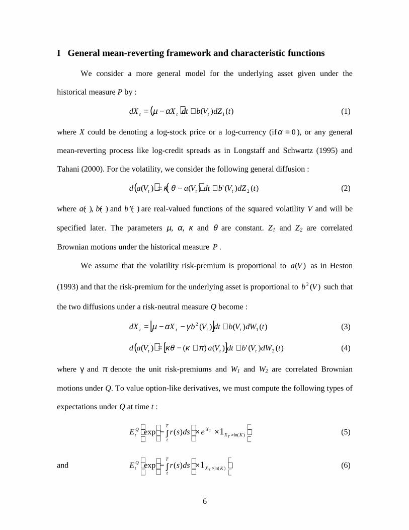
I General mean-reverting framework and characteristic functions
We consider a more general model for the underlying asset given under the
historical measure P by :
( ) )()( 1 tdZVbdtXdX ttt +−= αµ (1)
where X could be denoting a log-stock price or a log-currency (if0=α ), or any general
mean-reverting process like log-credit spreads as in Longstaff and Schwartz (1995) and
Tahani (2000). For the volatility, we consider the following general diffusion :
( ) ( ) )()(')()( 2 tdZVbdtVaVad ttt +−= θκ (2)
where a(· ), b(· ) and b’(· ) are real-valued functions of the squared volatility V and will be
specified later. The parameters µ, α, κ and θ are constant. Z1 and Z2 are correlated
Brownian motions under the historical measure P .
We assume that the volatility risk-premium is proportional to )(Va as in Heston
(1993) and that the risk-premium for the underlying asset is proportional to )(2 Vb such that
the two diffusions under a risk-neutral measure Q become :
[ ] )()()( 12 tdWVbdtVbXdX tttt +−−= γαµ (3)
( ) [ ] )()(')()()( 2 tdWVbdtVaVad ttt ++−= πκκθ (4)
where γ and π denote the unit risk-premiums and W1 and W2 are correlated Brownian
motions under Q. To value option-like derivatives, we must compute the following types of
expectations under Q at time t :
××
∫− > )ln(1)(exp KXX
T
t
Qt T
TedssrE (5)
and
×
∫− > )ln(1)(exp KX
T
t
Qt T
dssrE (6)
7
In order to obtain simpler expressions for these expectations, we consider two
probability measures Q1 and Q2 equivalent to Q and defined by their Radon-Nikodym
derivatives :
×
∫−
×
∫−=≡
T
T
XT
t
Qt
XT
t
edssrE
edssrTtg
dQ
dQ
)(exp
)(exp),(1
1 (7)
∫−
∫−=≡
T
t
Qt
T
t
dssrE
dssrTtg
dQ
dQ
)(exp
)(exp),(2
2 (8)
Q2 is simply the so-called T-forward measure. Equations (5) and (7) give :
( )
∫×>=
××
−
−
>∫ T
T
t
T
T Xdssr
QtTKX
XT
t
Qt eeEKXQedssrE
)(
1)ln( )ln()(exp 1 (9)
and Equations (6) and (8) give :
( ) ),()ln()(exp 2)ln(1 TtPKXQdssrE TKX
T
t
Qt T
×>=
×
− >∫ (10)
where P(t,T) denotes the zero-coupon bond maturing at T. We also define the characteristic
functions of the process X under Q1 and Q2 by :
( )[ ] 2,1forexp)( =≡ jXiEf T
Q
tjj φφ (11)
Expressed under the risk-neutral measure Q, the characteristic function1f becomes :
( )[ ]TQt XiTtgEf φφ exp),()( 11 ≡
( )
×
∫−
+×
∫−=
TXT
t
Qt
T
T
t
Qt
edssrE
XidssrE
)(exp
)1(exp)(exp φ (12)
8
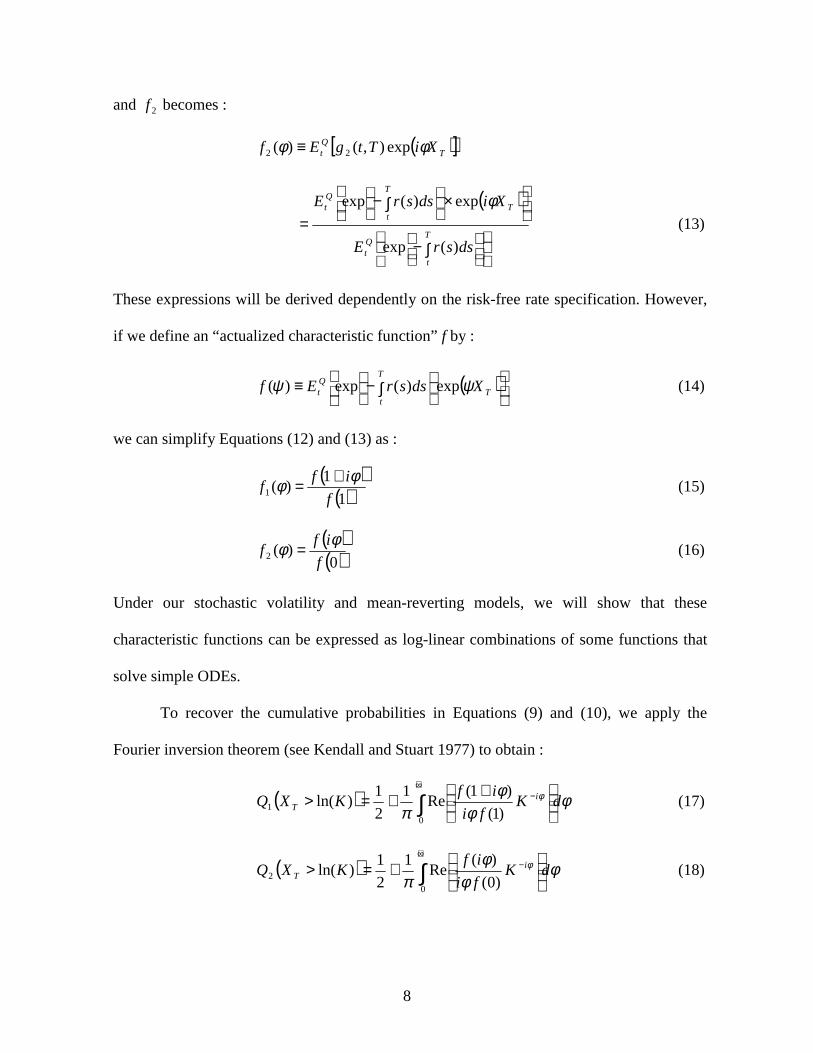
and 2f becomes :
( )[ ]TQt XiTtgEf φφ exp),()( 22 ≡
( )
∫−
×
∫−=
T
t
Qt
T
T
t
Qt
dssrE
XidssrE
)(exp
exp)(exp φ (13)
These expressions will be derived dependently on the risk-free rate specification. However,
if we define an “actualized characteristic function” f by :
( )
∫−≡ T
T
t
Qt XdssrEf ψψ exp)(exp)( (14)
we can simplify Equations (12) and (13) as :
( )
( )1
1)(1
f
iff
φφ += (15)
( )( )0
)(2f
iff
φφ = (16)
Under our stochastic volatility and mean-reverting models, we will show that these
characteristic functions can be expressed as log-linear combinations of some functions that
solve simple ODEs.
To recover the cumulative probabilities in Equations (9) and (10), we apply the
Fourier inversion theorem (see Kendall and Stuart 1977) to obtain :
( ) φφ
φπ
φ dKfi
ifKXQ i
T ∫+∞
−
++=>0
1 )1(
)1(Re
1
2
1)ln( (17)
( ) φφ
φπ
φ dKfi
ifKXQ i
T ∫+∞
−
+=>
0
2 )0(
)(Re
1
2
1)ln( (18)

9
where Re(· ) denotes the real part of a complex number. These integrals are well-defined (see
Appendix C) and convergent. Although they cannot be computed analytically, we will use
numerical techniques such as Gaussian quadrature to do it. The next section will consider
two different stochastic volatility models by choosing appropriate a(V) and b(V) functions
and derive their characteristic functions.
II Stochastic volatility models
II.1 Square-root mean-reverting model
In this subsection, we generalize Heston (1993) model by incorporating a mean-
reverting underlying asset. The model is given under the risk-neutral measure Q by :
( ) )(1 tdWVdtVXdX tttt +−−= γαµ (19)
( ) )(2 tdWVdtVdV ttt σλκθ +−= (20)
where dtWWdt
ρ=21, . For all models, we assume a constant risk-free rate denoted by r.
The characteristic function can be expressed by (for details, see Appendix A.1) :
( )( ) ( )
−−×
−
−−−+=
∫
−−
−−−−−−
T
t
sTQt
ttT
tTtTt
tT
XQt
dsVsTVE
Ve
eeXeeE T
)(exp
11exp
12
)(
)()()(
εε
ψσρ
ψακθ
σρψ
αµψ
α
ααα
ψ
(21)
where
( ) ( ) ( )
=
−−−−
+−=
ψσρε
ατρψατψγλασρτε
2
221 2exp1
2
1exp)()(
(22)
10
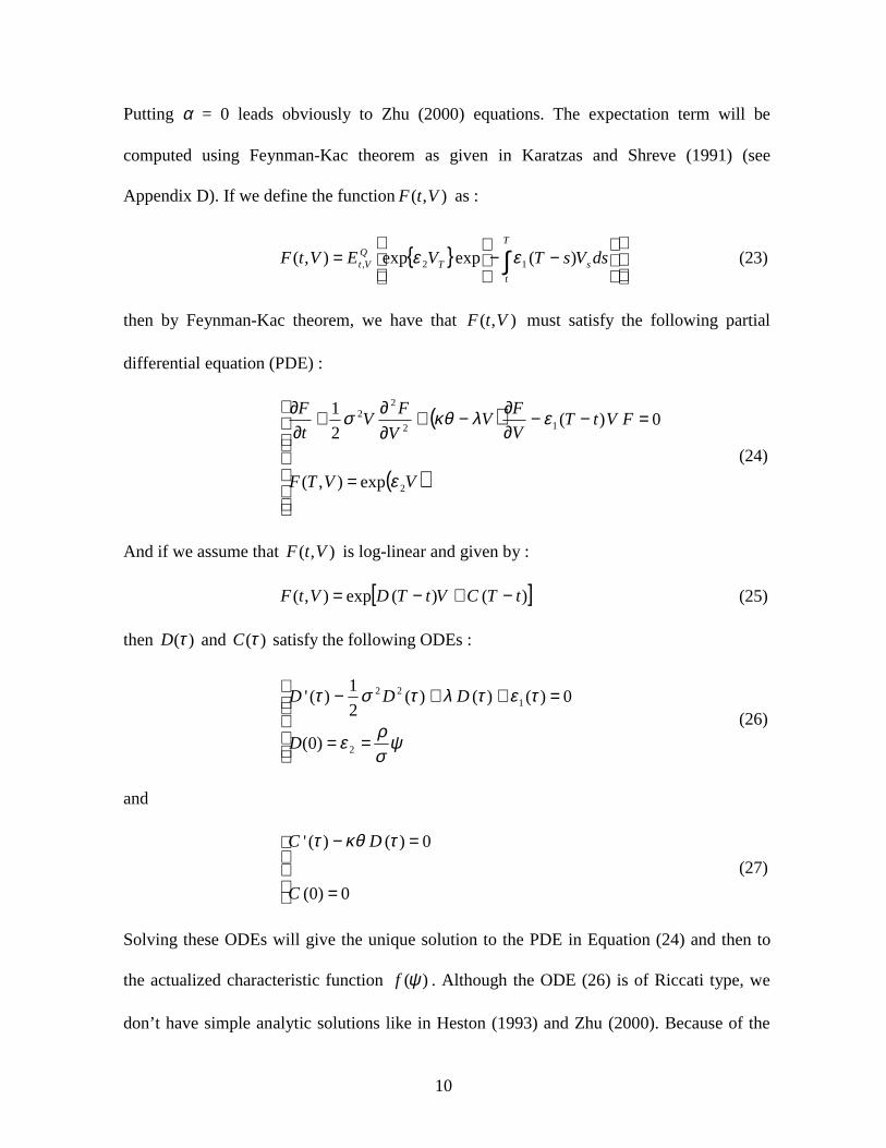
Putting α = 0 leads obviously to Zhu (2000) equations. The expectation term will be
computed using Feynman-Kac theorem as given in Karatzas and Shreve (1991) (see
Appendix D). If we define the function ),( VtF as :
{ }
−−= ∫T
t
sTQVt dsVsTVEVtF )(expexp),( 12, εε (23)
then by Feynman-Kac theorem, we have that ),( VtF must satisfy the following partial
differential equation (PDE) :
( )
( )
=
=−−∂∂−+
∂∂+
∂∂
VVTF
FVtTV
FV
V
FV
t
F
2
12
22
exp),(
0)(2
1
ε
ελκθσ
(24)
And if we assume that ),( VtF is log-linear and given by :
[ ])()(exp),( tTCVtTDVtF −+−= (25)
then )(τD and )(τC satisfy the following ODEs :
==
=++−
ψσρε
τετλτστ
2
122
)0(
0)()()(2
1)('
D
DDD (26)
and
=
=−
0)0(
0)()('
C
DC τκθτ (27)
Solving these ODEs will give the unique solution to the PDE in Equation (24) and then to
the actualized characteristic function )(ψf . Although the ODE (26) is of Riccati type, we
don’t have simple analytic solutions like in Heston (1993) and Zhu (2000). Because of the

11
mean-reverting feature, the function )(1 τε is of exponential type while it’s independent of
the time variable τ in Zhu (2000). However, these first-degree ODEs can be solved easily
using numerical methods such as Runge-Kutta formula or Adams-Bashforth-Moulton
method. For details about these methods, see Dormand and Prince (1980), Shampine (1994)
or Shampine and Gordon (1975).
The ODEs (26-27) have analytic solutions (given in Appendix A.2) that involve the
Whittaker functions. They need much more time (about 10 times on average) to be
computed for large values of φ (or equivalently ψ as defined in Equations 14-16) than
solved numerically for the same order of accuracy (the relative error is about 10-8). This may
be due to the fact that the confluent hypergeometric function is approximated by a series
expansion in all mathematical softwares and the calculation could be slow for large input
values (one could also face overflow errors as well). The series expansion for the Fong and
Vasicek (1992) discount bond price in Selby and Strickland (1995) is efficient because φ is
always equal to 1.
The actualized characteristic function )(ψf for the square-root mean-reverting
model is then given by :
( )
( ) ( )
[ ]);();(exp
11exp
exp)(exp)(
)(
)()()(
)(
ψψ
ψσρ
ψακθ
σρψ
αµψ
ψψ
α
ααα
tTCVtTD
Ve
eeXee
XdssrEf
t
ttT
tTtTt
tT
tTr
T
T
t
Qt
−+−×
−
−−−+×=
∫−≡
−−
−−−−−−
−− (28)
Now that we can evaluate numerically expressions like )( φif and )1( φif + for all
possible values of φ, we are able to compute cumulative probabilities under measures 1Q

12
and 2Q by inverting the Fourier transforms which leads to evaluate the integrals given in
Equations (17) and (18). This will be done by the Gaussian quadrature rule using Laguerre
polynomials. Section III will describe this method and shows how it applies to our models.
II.2 Ornstein-Uhlenbeck mean-reverting model
A. Risk-premium for the underlying asset is proportional to the squared volatility
In this subsection, we use an Ornstein-Uhlenbeck model for the volatility and a
mean-reverting underlying asset. The model is given under the risk-neutral measure Q by :
( ) )(12 tdWdtXdX tttt σγσαµ +−−= (29)
( ) )(2 tdWdtd tt βλσκθσ +−= (30)
where dtWWdt
ρ=21, . We can write the characteristic function as (for details, see
Appendix B) :
( )( ) ( )
−−−−×
−
−−−+=
∫∫
−−
−−−−−−
T
t
s
T
t
sTQt
ttT
tTtTt
tT
XQt
dssTdssTE
e
eeXe
eE T
212
23
2)(
)()()(
)()(exp
2
12
1
exp
σησηση
σψβρ
ψα
ρβψαµψ
α
ααα
ψ
(31)
where
( ) ( ) ( )
( )
=
−=
−−−−
+−=
ψβρη
ατψβ
ρκθτη
ατρψατψγβρλ
βαρτη
2
exp)(
2exp12
1exp
2)(
3
2
221
(32)
Again, putting 0=α leads to Zhu (2000) equations. Define the function ),( σtG as :
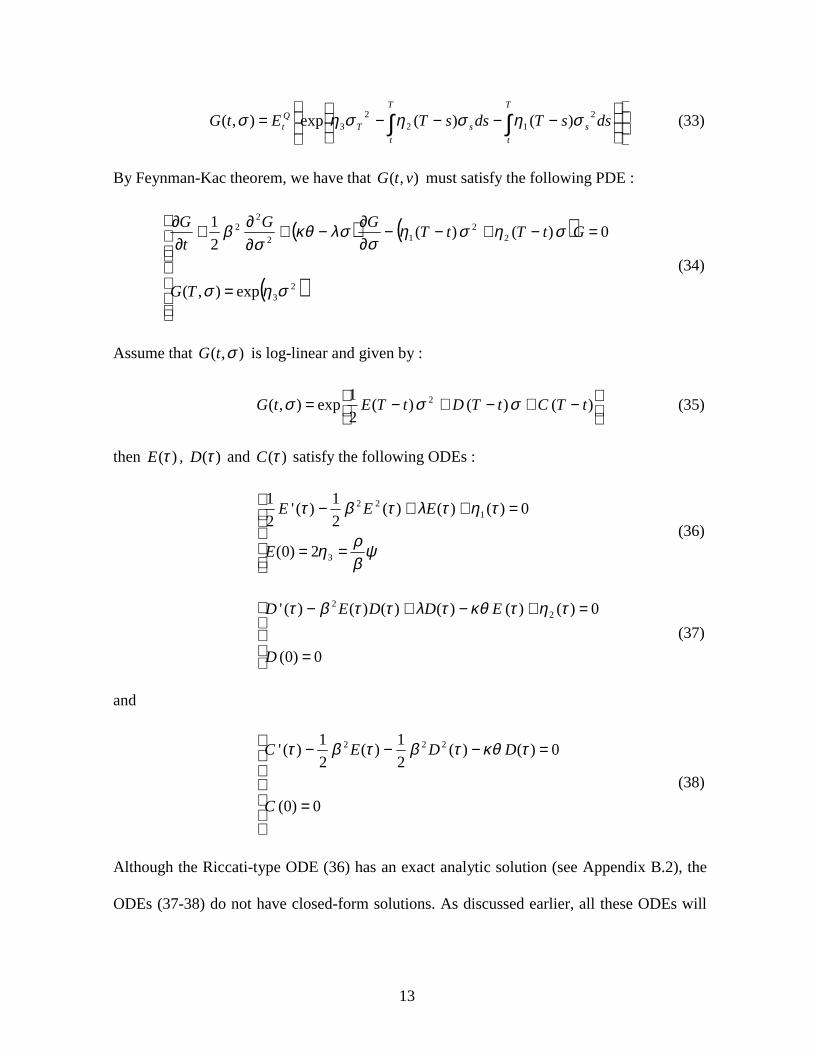
13
−−−−= ∫∫
T
t
s
T
t
sTQt dssTdssTEtG 2
122
3 )()(exp),( σησησησ (33)
By Feynman-Kac theorem, we have that ),( vtG must satisfy the following PDE :
( ) ( )
( )
=
=−+−−∂∂−+
∂∂+
∂∂
23
22
12
22
exp),(
0)()(2
1
σησ
σησησ
λσκθσ
β
TG
GtTtTGG
t
G
(34)
Assume that ),( σtG is log-linear and given by :
−+−+−= )()()(2
1exp),( 2 tTCtTDtTEtG σσσ (35)
then )(τE , )(τD and )(τC satisfy the following ODEs :
==
=++−
ψβρη
τητλτβτ
3
122
2)0(
0)()()(2
1)('
2
1
E
EEE
(36)
=
=+−+−
0)0(
0)()()()()()(' 22
D
EDDED τητκθτλττβτ (37)
and
=
=−−−
0)0(
0)()(2
1)(
2
1)(' 222
C
DDEC τκθτβτβτ
(38)
Although the Riccati-type ODE (36) has an exact analytic solution (see Appendix B.2), the
ODEs (37-38) do not have closed-form solutions. As discussed earlier, all these ODEs will

14
be solved numerically. The actualized characteristic function )(ψf for the Ornstein-
Uhlenbeck mean-reverting model is then given by :
( )
( ) ( )
−+−+−×
−
−−−+=
∫−≡
−−
−−−−−−
−−
);();();(2
1exp
2
12
1
exp
exp)(exp)(
2
2)(
)()()(
)(
ψσψσψ
σψβρ
ψα
ρβψαµψ
ψψ
α
ααα
tTCtTDtTE
e
eeXe
e
XdssrEf
tt
ttT
tTtTt
tT
tTr
T
T
t
Qt
(39)
B. Risk-premium for the underlying asset is proportional to the volatility
If the risk-premium for the underlying asset X is proportional to the volatility instead
of its square, the model’s equations become :
( ) )(1 tdWdtXdX tttt σγσαµ +−−= (40)
( ) )(2 tdWdtd tt βλσκθσ +−= (41)
and for the characteristic function, we obtain with the same calculations as before :
( )( ) ( )
−−−−×
−
−−−+=
∫∫
−−
−−−−−−
T
t
s
T
t
sTQt
ttT
tTtTt
tT
XQt
dssTdssTE
e
eeXe
eE T
212
23
2)(
)()()(
)()(exp
2
12
1
exp
σωσωσω
σψβρ
ψα
ρβψαµψ
α
ααα
ψ
(42)
where

15
( ) ( ) ( )
( )
=
−
+=
−−−−
−=
ψβρω
ατψγβ
ρκθτω
ατρψατψλαβρτω
2
exp)(
2exp12
1exp
2)(
3
2
221
(43)
Using Feynman-Kac theorem as before gives for the actualized characteristic function :
( )
( ) ( )
−+−+−×
−
−−−+=
∫−≡
−−
−−−−−−
−−
);();();(2
1exp
2
12
1
exp
exp)(exp)(
2
2)(
)()()(
)(
ψσψσψ
σψβρ
ψα
ρβψαµψ
ψψ
α
ααα
tTCtTDtTE
e
eeXe
e
XdssrEf
tt
ttT
tTtTt
tT
tTr
T
T
t
Qt
(44)
where functions )(),( ττ DE and )(τC solve the same ODEs in Equations (36-38) by
replacing 21,ηη and 3η respectively by 21,ωω and 3ω .
III Numerical integration using Gaussian quadrature
In general, a quadrature rule approximation allows to estimate an integral of a
function, )(φg , over a given interval with a linear combination of function values in the
interval [ ]ba, . After specifying a set of abscissas ( )njj ,...,1=
φ and their corresponding weights
( )njj ,...,1=
ω , the integral is approximated by :
∫ ∑=
≅b
a
n
jjj gdgw
1
)()()( φωφφφ (45)
where w is a weight function to be specified dependently on the rule which is used. The
abscissas and the weights are specified such that this approximation is exact for any given
16
polynomial function with a maximum degree. The highest degree is called the order of the
quadrature rule. While rules such as Trapezoidal and Simpson’s specify a set of equally
spaced abscissas and choose the weights to maximize the order, Gaussian rules determine
both abscissas and weights to maximize the order. For n abscissas and n weights, the highest
order is 12 −n . Furthermore, in many studies, Gaussian rules are shown to converge faster
than the classic Trapezoidal and Simpson’s rules and give greater accuracy even for small n
(Sullivan 2000).
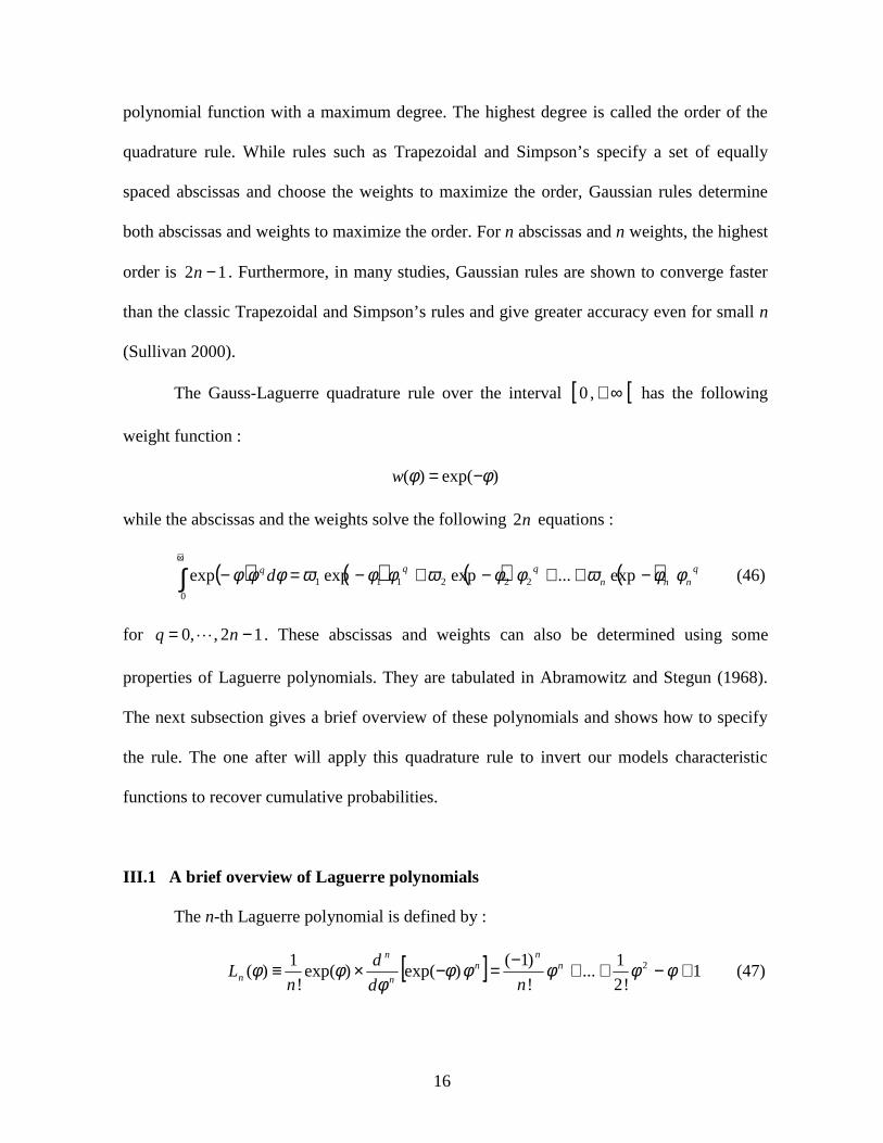
The Gauss-Laguerre quadrature rule over the interval [ [∞+,0 has the following
weight function :
)exp()( φφ −=w
while the abscissas and the weights solve the following n2 equations :
( ) ( ) ( ) ( ) qnnn
qqqd φφωφφωφφωφφφ −++−+−=−∫+∞
exp...expexpexp 222111
0
(46)
for 12,,0 −= nq � . These abscissas and weights can also be determined using some
properties of Laguerre polynomials. They are tabulated in Abramowitz and Stegun (1968).
The next subsection gives a brief overview of these polynomials and shows how to specify
the rule. The one after will apply this quadrature rule to invert our models characteristic
functions to recover cumulative probabilities.
III.1 A brief overview of Laguerre polynomials
The n-th Laguerre polynomial is defined by :
[ ] 1!2
1...
!
)1()exp()exp(
!
1)( 2 +−++−=−×≡ φφφφφ
φφφ n
nn
n
n
n nd
d
nL (47)

17
They have many characteristics, among which the “orthonormality” with respect to the
weight function :
=≠
==−∫+∞
pn
pndLL nppn if1
if0)()()exp(
0
δφφφφ (48)
where npδ is the Kronecker’s symbol. We can also proof that the n-th Lageurre polynomial
has exactly n real zeros over the interval ] [∞+,0 . These zeros are the abscissas, ( )njj ,...,1=
φ ,
needed for the Gauss-Laguerre quadrature rule of order n. The associated weights,
( )njj ,...,1=
ω , are then given by :
[ ] njLn
jn
j
j ,...,1)(
12
12
==− φ
φω (49)
In order to apply this integration method to our models, we need to modify the weights to
take into account the function to be integrated. Recall that we must value this type of
integrals :
[ ]
∑
∫∫
=
+∞+∞
≅
−=
n
jjjj g
dgdg
1
00
)()exp(
)()exp()exp()(
φφω
φφφφφφ (50)
While n increases, the sum converges to the true value if the function )()exp( φφ g satisfies
some assumptions as discussed in Davis and Rabinowitz (1984).
III.2 Recovering cumulative probabilities
For a fixed order n, we setup the abscissas ( )njj ,...,1=
φ and the modified weights
( )njjj ,...,1
)exp(=
φω as shown before. We also choose all the model’s parameters as well as

18
the time t, the maturity T, the strike K, the initial value for the underlying asset tX and,
depending on the model, the initial value for the volatility tσ or the squared volatility tV .
For every abscissa jφ or equivalently jψ as defined earlier by jj iφψ +=1 or by jj iφψ = ,
we solve the ODEs in Equations (26-27) for the square-root model and Equations (36-38)
for the Ornstein-Uhlenbeck model to get the functions values );( jtTE ψ− , );( jtTD ψ−
and );( jtTC ψ− defined in section II for every nj ,...,1= . We can then compute the
actualized characteristic functions values )( jf ψ at the needed points jψ and the
cumulative probabilities can then be approximated by :
( )
{ }∑
∫
=
+∞−
−
++≅
++=>
n
jj
j
j
jj
iT
Kifi
if
dKfi
ifKXQ
1
0
1
)ln(exp)1(
)1(Re)exp(
1
2
1
)1(
)1(Re
1
2
1)ln(
φφ
φφω
π
φφ
φπ
φ
(51)
and
( )
{ }∑
∫
=
+∞−
−+≅
+=>
n
jj
j
j
jj
iT
Kifi
if
dKfi
ifKXQ
1
0
2
)ln(exp)0(
)(Re)exp(
1
2
1
)0(
)(Re
1
2
1)ln(
φφ
φφω
π
φφ
φπ
φ
(52)
Theoretically, as n becomes large, these approximations converge to the true probability
values. As it will be shown with many valuation examples, a fast convergence and a good
accuracy can be achieved even with small n.

19
IV Credit spread options, caps, floors and swaps valuation
IV.1 Credit spread options
A credit spread option gives the right to buy or sell the credit at the strike price until
or at the expiration date dependently if the option is American or European. One could buy a
credit spread option for hedging its credit risk exposures against up or down movements in a
credit value as well as for speculative purposes. For an exhaustive credit derivatives
overview, see Howard (1995).
More specifically, denoting the maturity date by T and the strike by K, under the
models studied in earlier sections, the European Call premium is given by :
( ) ( ))ln()0;,()ln()1;,(),( ,2
,1 KXQKTtfKXQTtfTtCall T
TtT
Tt >−>= (53)
where the actualized characteristic function );,( ψTtf and the cumulative probabilities are
defined as before by :
( )
∫−= T
T
t
Qt XdssrETtf ψψ exp)(exp);,( (54)
and
( ) φφ
φπ
φ dKTtfi
iTtfKXQ i
TTt ∫
+∞−
++=>
0
,1 )1;,(
)1;,(Re
1
2
1)ln( (55)
( ) φφ
φπ
φ dKTtfi
iTtfKXQ i
TTt ∫
+∞−
+=>
0
,2 )0;,(
);,(Re
1
2
1)ln( (56)
The European Put can be derived using the Call-Put parity :
( ) ( ))ln()1;,()ln()0;,(),( ,1
,2 KXQTtfKXQKTtfTtPut T
TtT
Tt <−<= (57)
20
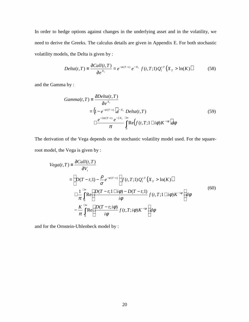
In order to hedge options against changes in the underlying asset and in the volatility, we
need to derive the Greeks. The calculus details are given in Appendix E. For both stochastic
volatility models, the Delta is given by :
( ))ln()1;,(),(
),( ,1
)( KXQTtfeee
TtCallTtDelta T
TtXtT
Xt
t>=
∂∂≡ −−−α (58)
and the Gamma by :
( )( )∫
∞+−
−−−
−−−
++
−=
∂∂≡
0
2)(2
)(
)1;,(Re
),(1
),(),(
φφπ
φα
α
dKiTtfee
TtDeltaee
e
TtDeltaTtGamma
iXtT
XtT
X
t
t
t
(59)
The derivation of the Vega depends on the stochastic volatility model used. For the square-
root model, the Vega is given by :
( )
∫
∫∞+
−
∞+−
−−
−−
+−−+−+
>
−−=
∂∂≡
0
0
,1
)(
);,();(
Re
)1;,()1;()1;(
Re1
)ln()1;,()1;(
),(),(
φφφ
φπ
φφφ
φπ
σρ
φ
φ
α
dKiTtfi
itTDK
dKiTtfi
tTDitTD
KXQTtfetTD
V
TtCallTtVega
i
i
TTttT
t
(60)
and for the Ornstein-Uhlenbeck model by :

21
( )
∫
∫
∞+−
∞+−
−−
−+−−
+
−−+−+
−−+−
+
>
−−+−=
∂∂≡
0
0
,1
)(
);,();();(
Re
)1;,()1;()1;(
)1;()1;(
Re1
)ln()1;,()1;()1;(
),(),(
φφφ
φσφ
φπ
φφ
φφ
σφ
φ
π
σβρσ
σ
φ
φ
α
dKiTtfi
itTD
i
itTEK
dKiTtf
i
tTDitTD
i
tTEitTE
KXQTtfetTDtTE
TtCallTtVega
it
i
t
TTt
ttT
t
t
(61)
IV.2 Credit spread Cap and Floor
A credit spread cap or floor provides the right to get payoffs at periodic dates called
the reset dates. At each reset date, the cap/floor payoff is the same as for a call/put. In this,
the cap/floor can be seen as a sequence of many calls/puts called caplets or floorlets. The
Figure below shows the reset dates and the associated payoffs for a credit spread cap with a
maturity T and different strike prices corresponding to the n periods.
The cap/floor premium is then equal to the sum of the corresponding caplets/floorlets
premia. The cap premium is given by :
( )
( )∑
∑
=
=
>−
>=
n
jjj
jjj
n
jjj
jj
KtXQKttf
KtXQttftCap
12
11
)ln()()0;,(
)ln()()1;,()(
(62)
{ }( )+− 11)(exp KtX { }( )+− 22)(exp KtX
Cap(t)
t = t0
t1 t2 T = tn
{ }( )+− nn KtX )(exp
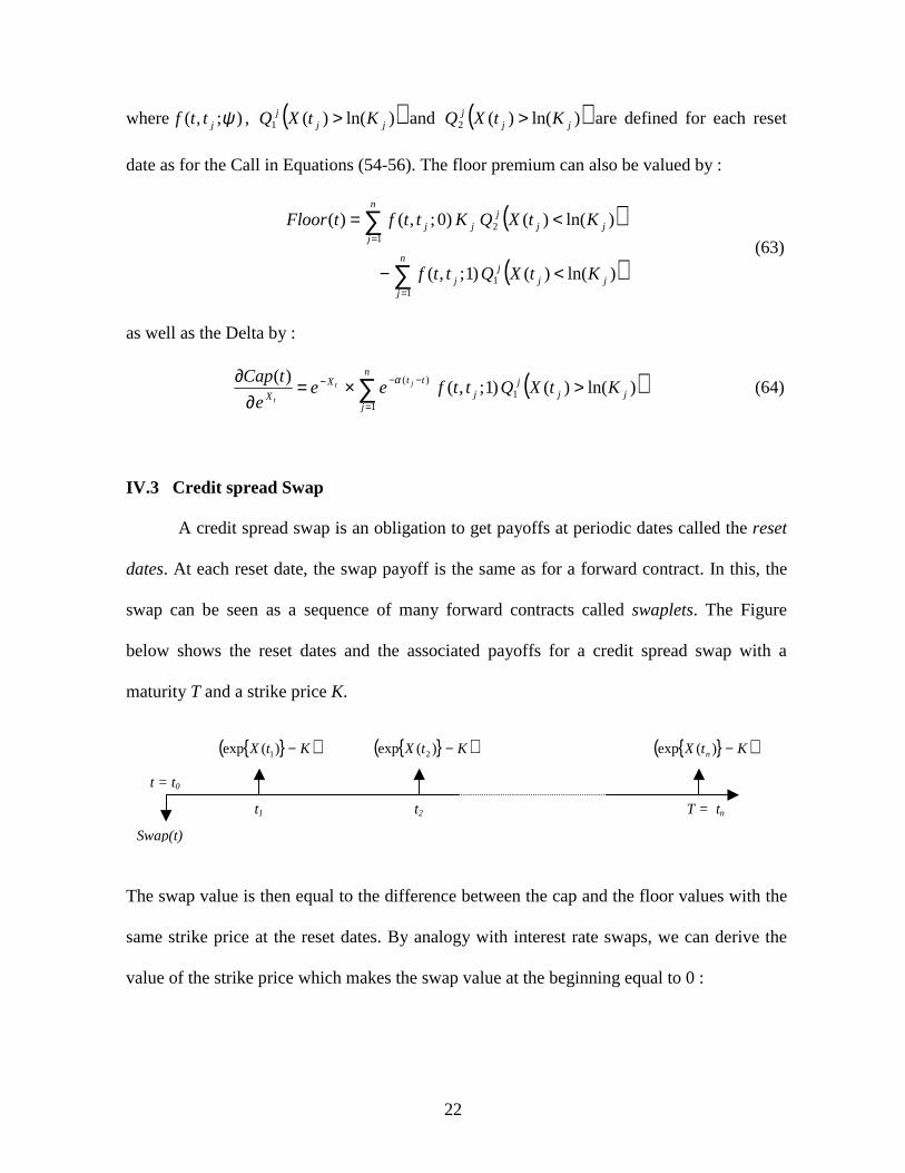
22
where );,( ψjttf , ( ))ln()(1 jjj KtXQ > and ( ))ln()(2 jj
j KtXQ > are defined for each reset
date as for the Call in Equations (54-56). The floor premium can also be valued by :
( )
( )∑
∑
=
=
<−
<=
n
jjj
jj
n
jjj
jjj
KtXQttf
KtXQKttftFloor
11
12
)ln()()1;,(
)ln()()0;,()(
(63)
as well as the Delta by :
( )∑=
−−− >×=∂
∂ n
jjj
jj
ttX
XKtXQttfee
e
tCap jt
t1
1)( )ln()()1;,(
)( α (64)
IV.3 Credit spread Swap
A credit spread swap is an obligation to get payoffs at periodic dates called the reset
dates. At each reset date, the swap payoff is the same as for a forward contract. In this, the
swap can be seen as a sequence of many forward contracts called swaplets. The Figure
below shows the reset dates and the associated payoffs for a credit spread swap with a
maturity T and a strike price K.
The swap value is then equal to the difference between the cap and the floor values with the
same strike price at the reset dates. By analogy with interest rate swaps, we can derive the
value of the strike price which makes the swap value at the beginning equal to 0 :
{ }( )KtX −)(exp 1 { }( )KtX −)(exp 2
Swap(t)
t = t0
t1 t2 T = tn
{ }( )KtX n −)(exp

23
∑
∑
=
== n
jj
n
jj
ttf
ttf
K
1
1
)0;,(
)1;,(
(65)
where );,( ψjttf are defined for each reset date as in Equation (54).
24
V Empirical results on convergence and the impact of mean-reversion
To assess the accuracy and the efficiency of our procedure, we priced many
European call options within different frameworks, Black and Scholes (1973) (B&S
hereafter), Longstaff and Schwartz (1995) (L&S hereafter) and Zhu (2000) (the Heston’s
(1993) model is one of the models studied by Zhu). For different parameters, we try to
converge to the exact true price. The true price for B&S and L&S frameworks are given by
the corresponding simple formula, while for Zhu framework, we use a Matlab® routine for
numerical integration.
The Tables 1 to 4 present the results for different maturities, different strikes and
different models parameters. All these applications show that a good accuracy is achieved
even with small quadrature rule order, between 10 and 15 depending on which model is used
and within which framework. We also find that the relative pricing errors are very small and
converge to 0. The Figures 1 to 4 present the relative errors. Notice that for Zhu (2000)
framework, the square-root model converges faster than the Ornstein-Uhlenbeck model.
The efficiency and the accuracy of our semi-analytic procedure within these “exact”
frameworks are still true for our mean-reverting frameworks. Indeed for both the square-root
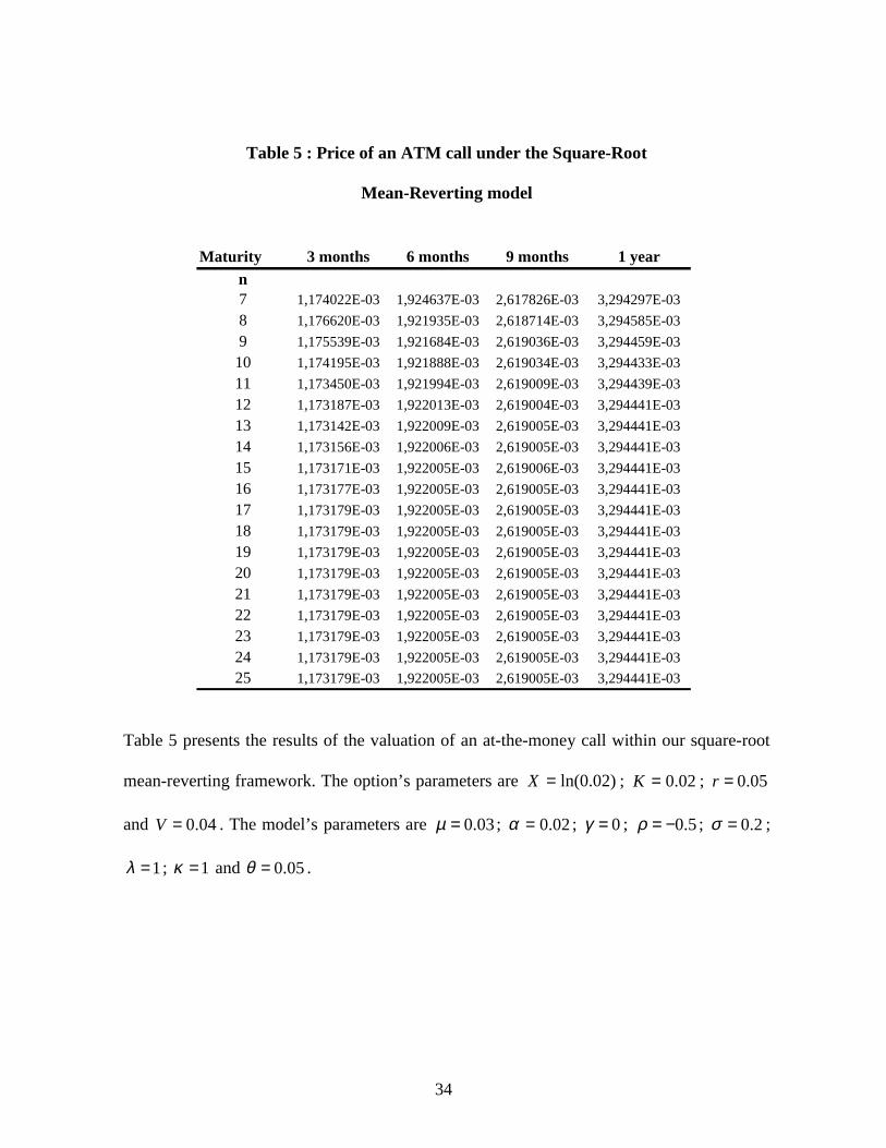
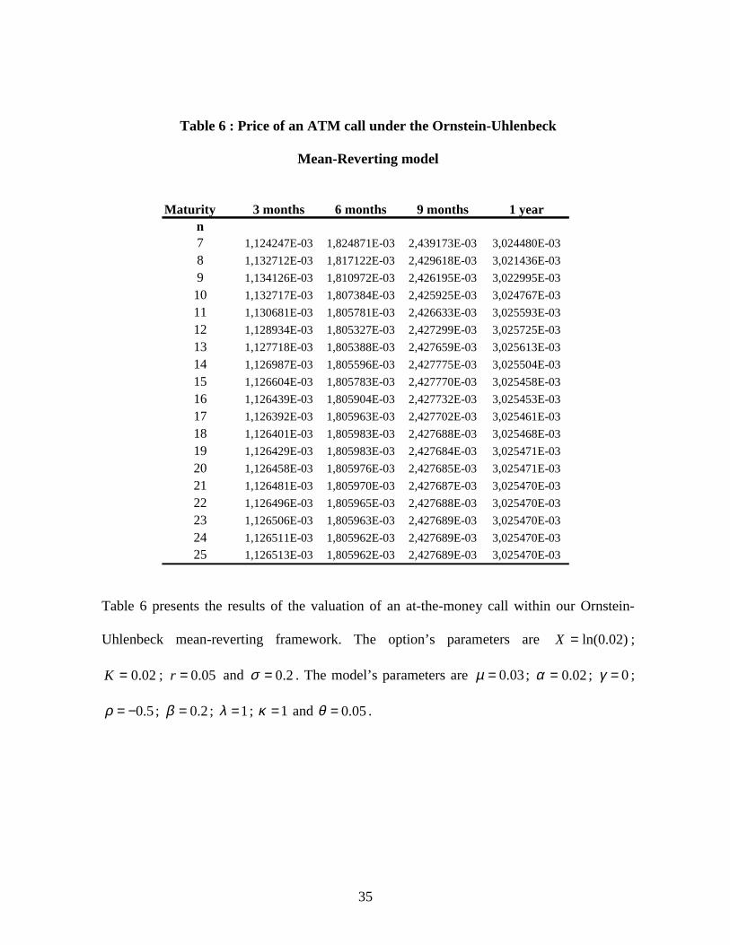
and the Ornstein-Uhlenbeck models, the “true” asymptotic price (this asymptotic price could
be computed with a Monte Carlo simulation) is attained for small quadrature rule orders
between 12 and 15. The Tables 5 and 6 present the convergence and the Figures 5 and 6
present the relative errors with respect to the asymptotic price. Again, the convergence is
faster for the square-root model than for the Ornstein-Uhlenbeck model.
We also show that the mean-reversion could have a large impact on option prices and
that is true even though the strength of the reversion is small. The results presented in Tables

25
7 and 8 show that with a small mean-reversion coefficient (for credit spreads, α is about
0.02), the relative impact with respect to the “no mean-reversion option price” (i.e. 0=α ) is
between 20% and 40% depending on the maturity.

26
VI Conclusion
In this paper, we propose semi-analytic pricing formulas for derivatives on mean-
reverting assets within two stochastic volatility frameworks. In this, we generalize Longstaff
and Schwartz (1995) by making the volatility stochastic; and Heston (1993) and Zhu (2000)
models by incorporating a mean-reverting component in the underlying asset diffusion. Our
work also extends the Fong and Vasicek (1992) model since we value options on general
mean-reverting underlying assets semi-analytically.
However, adding a mean-reverting feature in our models only allows getting a semi-
closed-form characteristic function, in the sense that we propose to solve some ODEs with
numerical methods like Runge-Kutta formula or Adams-Bashforth-Moulton method. In our
work, the numerical resolution is very accurate and takes much less time than the exact
computation since analytic solutions (when they exist) involve complex algebra with
Whittaker and the confluent hypergeometric functions. The use of numerical integration
method, like the Gaussian-Laguerre quadrature rule, to invert the characteristic function is
necessary to recover cumulative probabilities and then to price derivatives. With some
pricing applications within different frameworks as Black and Scholes (1973), Longstaff and
Schwartz (1995), Heston (1993) and Zhu (2000), it is shown that a good accuracy is
achieved even with small quadrature rule orders and that the relative pricing errors are very
small and convergent to 0. These results also apply to our mean-reverting frameworks, the
prices converge to asymptotic prices and the relative errors are small and tend to 0.
As particular applications to our general valuation models, we derive semi-closed-
form pricing formulas for credit-spread European options, caps, floors and swaps. We also
show an interesting feature of derivative prices on mean-reverting assets. We find that the

27
impact of small reversion coefficients on the prices could be very large. This finding proves
that the pricing of derivatives on mean-reverting underlying assets is very sensitive to the
strength of the reversion and that has to be taken into account.
The combination of numerical resolution of ODEs with numerical integration using
Gaussian-Laguerre quadrature rule provides extremely accurate valuation of credit
derivatives and may do well for derivatives on other mean-reverting underlying assets like
interest rates and commodities.

28
References
Abramowitz M., and I. Stegun, 1968. Handbook of Mathematical Functions (5th Edition), Dover Publications, Inc., New York.
Bates D., 1996, “Jumps and Stochastic Volatility: Exchange Rate Processes Implicit in Deutsche Mark Options,” The Review of Financial Studies, Vol 9, 69-107.
Bakshi G., C. Cao, and Z. Chen, 1997, “Empirical Performance of Alternative Option Pricing Models,” The Journal of Finance, Vol 52, 2003-2049.
Black F., and M. Scholes, 1973, “The Valuation of Options and Corporate Liabilities,” Journal of Political Economy, Vol 81, 637-654.
Clewlow L. J., and C. R. Strickland, 1997, “Monte Carlo Valuation of Interest Rate Derivatives under Stochastic Volatility,” The Journal of Fixed Income, Vol 7, 35-45.
Cox J., J. Ingersoll, and S. Ross, 1985, “A Theory of the Term Structure of Interest Rates,” Econometrica, Vol 53, 385-407.
Davis P., and P. Rabinowitz, 1984. Methods of Numerical Integration (2nd Edition), Academic Press, Inc., California.
Dormand, J. R. and P. J. Prince, 1980, “A family of embedded Runge-Kutta formulae,” Journal of Computation and Applied Mathematics, Vol 6, 19-26.
Duan J.C., 1995, “The GARCH Option Pricing Model,” Mathematical Finance, Vol 5, 13-32.
Feller W., 1966. An Introduction to Probability Theory and Its Applications (Vol 2), Wiley & Sons, New York.
Fong H.G., and O. A. Vasicek, 1992, “Interest Rate Volatility as a Stochastic Factor,” Working paper, Gifford Associates.
Heston S.L., 1993, “A Closed-Form Solution for Options with Stochastic Volatility, with Applications to Bond and Currency Options,” The Review of Financial Studies, Vol 6, 327-343.
Heston S.L., and S. Nandi, 2000, “A Closed-Form GARCH Option Valuation Model,” The Review of Financial Studies, Vol 13, 585-625.
29
Howard K., 1995, “An Introduction to Credit Derivatives,” Derivatives Quarterly, Vol 2, 28-37.
Kendall M., and A. Stuart, 1977. The Advanced Theory of Statistics (Vol 1), Macmillan Publishing Co., Inc., New York.
Karatzas I., and S.A. Shreve, 1991. Brownian Motion and Stochastic Calculus, Springer Verlag, New York.
Longstaff F.A., and E.S. Schwartz, 1995, “Valuing Credit Derivatives,” The Journal of Fixed Income, Vol 5, 6-12.
Schöbel R., and J. Zhu, 1998, “Stochastic Volatility With an Ornstein-Uhlenbeck Process : An Extension,” Working paper, Eberhard-Karls-Universität Tübingen.
Schwartz E.S., 1997, “The Stochastic Behavior of Commodity Prices: Implications for Valuation and Hedging,” The Journal of Finance, Vol 3, 6-12.
Selby M. J. P., and C. R. Strickland, 1995, “Computing the Fong and Vasicek Pure Discount Bond Price Formula,” The Journal of Fixed Income, Vol 5, 78-84.
Shampine L. F., 1994. Numerical Solution of Ordinary Differential Equations, Chapman & Hall, New York.
Shampine L. F., and M. K. Gordon, 1975. Computer Solution of Ordinary Differential Equations: the Initial Value Problem, W. H. Freeman, San Francisco.
Sullivan M.A., 2000, “Valuing American Put Options Using Gaussian Quadrature,” The Review of Financial Studies, Vol 13, 75-94.
Tahani N., 2000, “Credit Spread Option Valuation under GARCH,” Working paper, Risk Management Chair, HEC Montreal.
Vasicek O.A., 1977, “An Equilibrium Characterization of the Term Structure,” Journal of Financial Economics, Vol 5, 177-188.
Zhu J., 2000, “Modular Pricing of Options,” Working paper, Eberhard-Karls-Universität Tübingen.

30
Tables
Table 1 : Convergence to B&S ATM call
Table 1 presents the results of the valuation of an at-the-money call within Black and
Scholes (1973) framework both with the B&S analytic formula and with our numerical
procedure. The option’s parameters are )100ln(=X ; 100=K ; 05.0=r and 04.0=V . To
match B&S framework, the model’s parameters are r=µ ; 0=α ; 5.0=γ ; 0=ρ ; 0=σ ;
0=λ ; 0=κ and 0=θ .
Maturity 3 months 6 months 9 months 1 year
B&S price 4,614997 6,888729 8,772268 10,450584
n7 4,576689 6,888989 8,772230 10,450610
8 4,605435 6,888729 8,772276 10,450578
9 4,613204 6,888726 8,772267 10,450584
10 4,614770 6,888729 8,772268 10,450583
11 4,614983 6,888729 8,772268 10,450584
12 4,614998 6,888729 8,772268 10,450584
13 4,614997 6,888729 8,772268 10,450584
14 4,614997 6,888729 8,772268 10,450584
15 4,614997 6,888729 8,772268 10,450584
16 4,614997 6,888729 8,772268 10,450584
17 4,614997 6,888729 8,772268 10,450584
18 4,614997 6,888729 8,772268 10,450584
19 4,614997 6,888729 8,772268 10,450584
20 4,614997 6,888729 8,772268 10,450584
21 4,614997 6,888729 8,772268 10,450584
22 4,614997 6,888729 8,772268 10,450584
23 4,614997 6,888729 8,772268 10,450584
24 4,614997 6,888729 8,772268 10,450584
25 4,614997 6,888729 8,772268 10,450584

31
Table 2 : Convergence to L&S ATM call
Table 2 presents the results of the valuation of an at-the-money call within Longstaff and
Schwartz (1995) framework both with the L&S analytic formula and with our numerical
procedure. The option’s parameters are )02.0ln(=X ; 02.0=K ; 05.0=r and 04.0=V .
To match L&S framework, the model’s parameters are 02.0=µ ; 015.0=α ; 0=γ ;
0=ρ ; 0=σ ; 0=λ ; 0=κ and 0=θ .
Maturity 3 months 6 months 9 months 1 year
L&S price 1,066132E-03 1,681529E-03 2,229959E-03 2,746019E-03
n7 1,059709E-03 1,681586E-03 2,229965E-03 2,746012E-03
8 1,064684E-03 1,681522E-03 2,229960E-03 2,746019E-03
9 1,065903E-03 1,681529E-03 2,229959E-03 2,746018E-03
10 1,066112E-03 1,681529E-03 2,229959E-03 2,746019E-03
11 1,066132E-03 1,681529E-03 2,229959E-03 2,746019E-03
12 1,066132E-03 1,681529E-03 2,229959E-03 2,746019E-03
13 1,066132E-03 1,681529E-03 2,229959E-03 2,746019E-03
14 1,066132E-03 1,681529E-03 2,229959E-03 2,746019E-03
15 1,066132E-03 1,681529E-03 2,229959E-03 2,746019E-03
16 1,066132E-03 1,681529E-03 2,229959E-03 2,746019E-03
17 1,066132E-03 1,681529E-03 2,229959E-03 2,746019E-03
18 1,066132E-03 1,681529E-03 2,229959E-03 2,746019E-03
19 1,066132E-03 1,681529E-03 2,229959E-03 2,746019E-03
20 1,066132E-03 1,681529E-03 2,229959E-03 2,746019E-03
21 1,066132E-03 1,681529E-03 2,229959E-03 2,746019E-03
22 1,066132E-03 1,681529E-03 2,229959E-03 2,746019E-03
23 1,066131E-03 1,681529E-03 2,229959E-03 2,746019E-03
24 1,066131E-03 1,681529E-03 2,229959E-03 2,746019E-03
25 1,066131E-03 1,681529E-03 2,229959E-03 2,746019E-03

32
Table 3 : Convergence to Zhu Square-Root ATM call
Table 3 presents the results of the valuation of an at-the-money call within Zhu (2000)
framework both with the Zhu square-root semi-analytic formula and with our numerical
procedure. The option’s parameters are )100ln(=X ; 100=K ; 05.0=r and 04.0=V . To
match Zhu framework, the model’s parameters are r=µ ; 0=α ; 5.0=γ ; 5.0−=ρ ;
1.0=σ ; 4=λ ; 4=κ and 06.0=θ .
Maturity 3 months 6 months 9 months 1 year
Zhu price 4,962005 7,620725 9,824956 11,766004
n7 4,947824 7,620594 9,825099 11,765874
8 4,961141 7,620671 9,824932 11,766032
9 4,962557 7,620737 9,824959 11,765998
10 4,962208 7,620725 9,824955 11,766006
11 4,962029 7,620725 9,824956 11,766004
12 4,962002 7,620725 9,824956 11,766004
13 4,962004 7,620725 9,824956 11,766004
14 4,962005 7,620725 9,824956 11,766004
15 4,962005 7,620725 9,824956 11,766004
16 4,962005 7,620725 9,824956 11,766004
17 4,962005 7,620725 9,824956 11,766004
18 4,962005 7,620725 9,824956 11,766004
19 4,962005 7,620725 9,824956 11,766004
20 4,962005 7,620725 9,824956 11,766004
21 4,962005 7,620725 9,824956 11,766004
22 4,962005 7,620725 9,824956 11,766004
23 4,962005 7,620725 9,824956 11,766004
24 4,962005 7,620725 9,824956 11,766004
25 4,962005 7,620725 9,824956 11,766004

33
Table 4 : Convergence to Zhu Ornstein-Uhlenbeck ATM call
Table 4 presents the results of the valuation of an at-the-money call within Zhu (2000)
framework both with the Zhu Ornstein-Uhlenbeck semi-analytic formula and with our
numerical procedure. The option’s parameters are )100ln(=X ; 100=K ; 05.0=r and
2.0=σ . To match Zhu framework, the model’s parameters are r=µ ; 0=α ; 5.0=γ ;
5.0−=ρ ; 1.0=β ; 4=λ ; 4=κ and 06.0=θ .
Maturity 3 months 6 months 9 months 1 yearZhu price 3,692764 4,977335 6,056673 7,089761
n7 3,524815 4,940583 6,081476 7,143954
8 3,619622 4,985383 6,089360 7,124454
9 3,668585 4,994529 6,077641 7,103581
10 3,690008 4,990486 6,065813 7,092411
11 3,696937 4,984396 6,059099 7,088899
12 3,697505 4,980122 6,056573 7,088730
13 3,696076 4,977996 6,056122 7,089273
14 3,694563 4,977249 6,056309 7,089642
15 3,693544 4,977128 6,056528 7,089772
16 3,693010 4,977196 6,056643 7,089787
17 3,692792 4,977273 6,056680 7,089775
18 3,692731 4,977317 6,056683 7,089765
19 3,692730 4,977335 6,056679 7,089761
20 3,692744 4,977339 6,056676 7,089761
21 3,692755 4,977338 6,056674 7,089761
22 3,692761 4,977337 6,056674 7,089761
23 3,692763 4,977336 6,056673 7,089761
24 3,692764 4,977336 6,056673 7,089761
25 3,692764 4,977335 6,056673 7,089761
34
Table 5 : Price of an ATM call under the Square-Root
Mean-Reverting model
Table 5 presents the results of the valuation of an at-the-money call within our square-root
mean-reverting framework. The option’s parameters are )02.0ln(=X ; 02.0=K ; 05.0=r
and 04.0=V . The model’s parameters are 03.0=µ ; 02.0=α ; 0=γ ; 5.0−=ρ ; 2.0=σ ;
1=λ ; 1=κ and 05.0=θ .
Maturity 3 months 6 months 9 months 1 yearn7 1,174022E-03 1,924637E-03 2,617826E-03 3,294297E-03
8 1,176620E-03 1,921935E-03 2,618714E-03 3,294585E-03
9 1,175539E-03 1,921684E-03 2,619036E-03 3,294459E-03
10 1,174195E-03 1,921888E-03 2,619034E-03 3,294433E-03
11 1,173450E-03 1,921994E-03 2,619009E-03 3,294439E-03
12 1,173187E-03 1,922013E-03 2,619004E-03 3,294441E-03
13 1,173142E-03 1,922009E-03 2,619005E-03 3,294441E-03
14 1,173156E-03 1,922006E-03 2,619005E-03 3,294441E-03
15 1,173171E-03 1,922005E-03 2,619006E-03 3,294441E-03
16 1,173177E-03 1,922005E-03 2,619005E-03 3,294441E-03
17 1,173179E-03 1,922005E-03 2,619005E-03 3,294441E-03
18 1,173179E-03 1,922005E-03 2,619005E-03 3,294441E-03
19 1,173179E-03 1,922005E-03 2,619005E-03 3,294441E-03
20 1,173179E-03 1,922005E-03 2,619005E-03 3,294441E-03
21 1,173179E-03 1,922005E-03 2,619005E-03 3,294441E-03
22 1,173179E-03 1,922005E-03 2,619005E-03 3,294441E-03
23 1,173179E-03 1,922005E-03 2,619005E-03 3,294441E-03
24 1,173179E-03 1,922005E-03 2,619005E-03 3,294441E-03
25 1,173179E-03 1,922005E-03 2,619005E-03 3,294441E-03
35
Table 6 : Price of an ATM call under the Ornstein-Uhlenbeck
Mean-Reverting model
Table 6 presents the results of the valuation of an at-the-money call within our Ornstein-
Uhlenbeck mean-reverting framework. The option’s parameters are )02.0ln(=X ;
02.0=K ; 05.0=r and 2.0=σ . The model’s parameters are 03.0=µ ; 02.0=α ; 0=γ ;
5.0−=ρ ; 2.0=β ; 1=λ ; 1=κ and 05.0=θ .
Maturity 3 months 6 months 9 months 1 yearn7 1,124247E-03 1,824871E-03 2,439173E-03 3,024480E-03
8 1,132712E-03 1,817122E-03 2,429618E-03 3,021436E-03
9 1,134126E-03 1,810972E-03 2,426195E-03 3,022995E-03
10 1,132717E-03 1,807384E-03 2,425925E-03 3,024767E-03
11 1,130681E-03 1,805781E-03 2,426633E-03 3,025593E-03
12 1,128934E-03 1,805327E-03 2,427299E-03 3,025725E-03
13 1,127718E-03 1,805388E-03 2,427659E-03 3,025613E-03
14 1,126987E-03 1,805596E-03 2,427775E-03 3,025504E-03
15 1,126604E-03 1,805783E-03 2,427770E-03 3,025458E-03
16 1,126439E-03 1,805904E-03 2,427732E-03 3,025453E-03
17 1,126392E-03 1,805963E-03 2,427702E-03 3,025461E-03
18 1,126401E-03 1,805983E-03 2,427688E-03 3,025468E-03
19 1,126429E-03 1,805983E-03 2,427684E-03 3,025471E-03
20 1,126458E-03 1,805976E-03 2,427685E-03 3,025471E-03
21 1,126481E-03 1,805970E-03 2,427687E-03 3,025470E-03
22 1,126496E-03 1,805965E-03 2,427688E-03 3,025470E-03
23 1,126506E-03 1,805963E-03 2,427689E-03 3,025470E-03
24 1,126511E-03 1,805962E-03 2,427689E-03 3,025470E-03
25 1,126513E-03 1,805962E-03 2,427689E-03 3,025470E-03
36
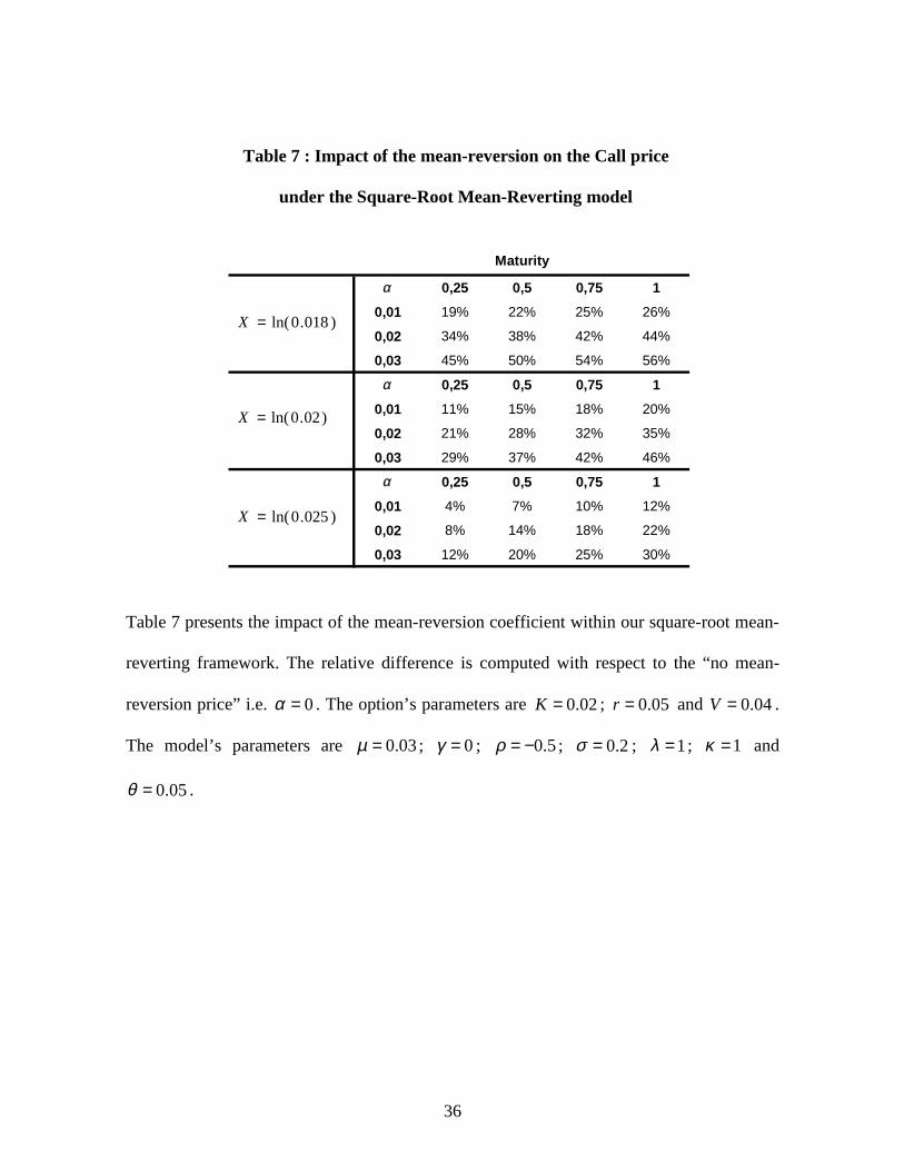
Table 7 : Impact of the mean-reversion on the Call price
under the Square-Root Mean-Reverting model
Table 7 presents the impact of the mean-reversion coefficient within our square-root mean-
reverting framework. The relative difference is computed with respect to the “no mean-
reversion price” i.e. 0=α . The option’s parameters are 02.0=K ; 05.0=r and 04.0=V .
The model’s parameters are 03.0=µ ; 0=γ ; 5.0−=ρ ; 2.0=σ ; 1=λ ; 1=κ and
05.0=θ .
α 0,25 0,5 0,75 1
0,01 19% 22% 25% 26%
0,02 34% 38% 42% 44%
0,03 45% 50% 54% 56%
α 0,25 0,5 0,75 1
0,01 11% 15% 18% 20%
0,02 21% 28% 32% 35%
0,03 29% 37% 42% 46%
α 0,25 0,5 0,75 1
0,01 4% 7% 10% 12%
0,02 8% 14% 18% 22%
0,03 12% 20% 25% 30%
Maturity
)018.0ln(=X
)025.0ln(=X
)02.0ln(=X

37
Table 8 : Impact of the mean-reversion on the Call price
under the Ornstein-Uhlenbeck Mean-Reverting model
Table 8 presents the impact of the mean-reversion coefficient within our Ornstein-
Uhlenbeck mean-reverting framework. The relative difference is computed with respect to
the “no mean-reversion price” i.e. 0=α . The option’s parameters are 02.0=K ; 05.0=r
and 04.0=V . The model’s parameters are 03.0=µ ; 0=γ ; 5.0−=ρ ; 2.0=β ; 1=λ ;
1=κ and 05.0=θ .
α 0,25 0,5 0,75 1
0,01 22% 27% 31% 34%
0,02 38% 46% 50% 54%
0,03 50% 58% 63% 66%
α 0,25 0,5 0,75 1
0,01 12% 18% 21% 24%
0,02 23% 31% 36% 40%
0,03 31% 41% 47% 52%
α 0,25 0,5 0,75 1
0,01 4% 7% 10% 13%
0,02 8% 14% 19% 23%
0,03 12% 20% 26% 31%
Maturity
)018.0ln(=X
)025.0ln(=X
)02.0ln(=X

38
Figures
Figure 1 : B&S call pricing relative error
Figure 1 shows the relative pricing error of a call within Black and Scholes (B&S)
framework. The true price is given by B&S analytic formula. The underlying asset values
are )100ln(=X ; )110ln(=X and )90ln(=X . The option’s parameters are 100=K ;
5.0=T ; 05.0=r and 04.0=V . To match B&S framework, the model’s parameters are
r=µ ; 0=α ; 5.0=γ ; 0=ρ ; 0=σ ; 0=λ ; 0=κ and 0=θ .
0,00E+00
1,00E-05
2,00E-05
3,00E-05
4,00E-05
5,00E-05
6,00E-05
7,00E-05
8,00E-05
7 8 9 10 11 12 13 14 15 16 17 18 19 20 21 22 23 24 25
Quadrature rule order
Rel
ativ
e er
ror
ATM call relative error ITM call relative error OTM call relative error
39
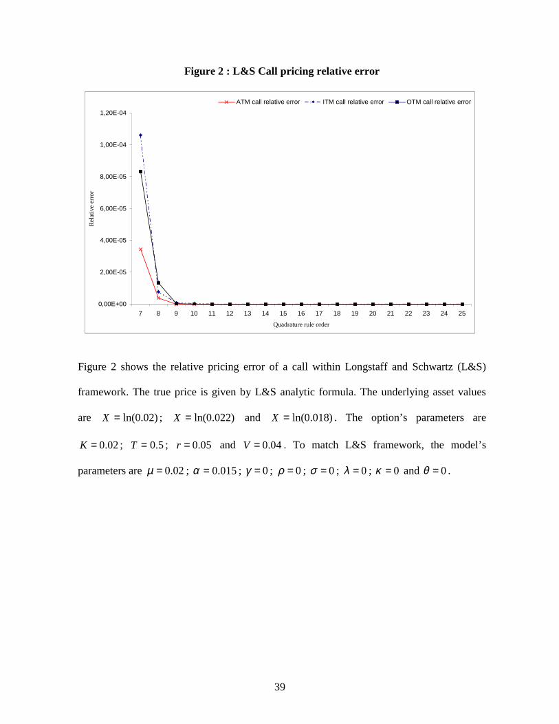
Figure 2 : L&S Call pricing relative error
Figure 2 shows the relative pricing error of a call within Longstaff and Schwartz (L&S)
framework. The true price is given by L&S analytic formula. The underlying asset values
are )02.0ln(=X ; )022.0ln(=X and )018.0ln(=X . The option’s parameters are
02.0=K ; 5.0=T ; 05.0=r and 04.0=V . To match L&S framework, the model’s
parameters are 02.0=µ ; 015.0=α ; 0=γ ; 0=ρ ; 0=σ ; 0=λ ; 0=κ and 0=θ .
0,00E+00
2,00E-05
4,00E-05
6,00E-05
8,00E-05
1,00E-04
1,20E-04
7 8 9 10 11 12 13 14 15 16 17 18 19 20 21 22 23 24 25
Quadrature rule order
Rel
ativ
e er
ror
ATM call relative error ITM call relative error OTM call relative error

40
Figure 3 : Zhu square-root Call pricing relative error
Figure 3 shows the relative pricing error of a call within Zhu framework. The true price is
given by Zhu square-root semi-analytic formula. The underlying asset values are
)100ln(=X ; )120ln(=X and )80ln(=X . The option’s parameters are 100=K ; 5.0=T ;
05.0=r and 04.0=V . To match Zhu framework, the model’s parameters are 05.0=µ ;
0=α ; 5.0=γ ; 5.0−=ρ ; 1.0=σ ; 4=λ ; 4=κ and 06.0=θ .
0,00E+00
5,00E-05
1,00E-04
1,50E-04
2,00E-04
2,50E-04
3,00E-04
7 8 9 10 11 12 13 14 15 16 17 18 19 20 21 22 23 24 25
Quadrature rule order
Rel
ativ
e er
ror
ATM call relative error ITM call relative error OTM call relative error

41
Figure 4 : Zhu Ornstein-Uhlenbeck Call pricing relative error
Figure 4 shows the relative pricing error of a call within Zhu framework. The true price is
given by Zhu Ornstein-Uhlenbeck semi-analytic formula. The underlying asset values are
)100ln(=X ; )120ln(=X and )80ln(=X . The option’s parameters are 100=K ; 1=T ;
05.0=r and 2.0=σ . To match Zhu framework, the model’s parameters are 05.0=µ ;
0=α ; 5.0=γ ; 5.0−=ρ ; 1.0=β ; 4=λ ; 4=κ and 06.0=θ . To keep the same scale, the
out-of-the-money pricing relative error is divided by 50.
0,00E+00
2,00E-03
4,00E-03
6,00E-03
8,00E-03
1,00E-02
1,20E-02
7 8 9 10 11 12 13 14 15 16 17 18 19 20 21 22 23 24 25
Quadrature rule order
Re
lativ
e e
rror
ATM call relative error ITM call relative error OTM call relative error
42
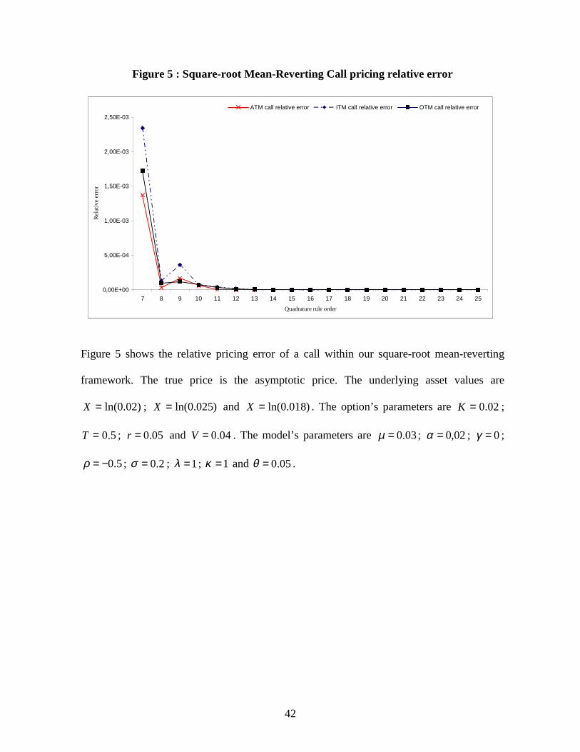
Figure 5 : Square-root Mean-Reverting Call pricing relative error
Figure 5 shows the relative pricing error of a call within our square-root mean-reverting
framework. The true price is the asymptotic price. The underlying asset values are
)02.0ln(=X ; )025.0ln(=X and )018.0ln(=X . The option’s parameters are 02.0=K ;
5.0=T ; 05.0=r and 04.0=V . The model’s parameters are 03.0=µ ; 02,0=α ; 0=γ ;
5.0−=ρ ; 2.0=σ ; 1=λ ; 1=κ and 05.0=θ .
0,00E+00
5,00E-04
1,00E-03
1,50E-03
2,00E-03
2,50E-03
7 8 9 10 11 12 13 14 15 16 17 18 19 20 21 22 23 24 25
Quadrature rule order
Re
lativ
e e
rror
ATM call relative error ITM call relative error OTM call relative error
43
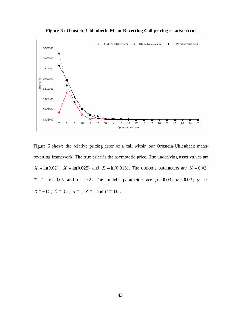
Figure 6 : Ornstein-Uhlenbeck Mean-Reverting Call pricing relative error
Figure 6 shows the relative pricing error of a call within our Ornstein-Uhlenbeck mean-
reverting framework. The true price is the asymptotic price. The underlying asset values are
)02.0ln(=X ; )025.0ln(=X and )018.0ln(=X . The option’s parameters are 02.0=K ;
1=T ; 05.0=r and 2.0=σ . The model’s parameters are 03.0=µ ; 02,0=α ; 0=γ ;
5.0−=ρ ; 2.0=β ; 1=λ ; 1=κ and 05.0=θ .
0,00E+00
5,00E-04
1,00E-03
1,50E-03
2,00E-03
2,50E-03
3,00E-03
3,50E-03
7 8 9 10 11 12 13 14 15 16 17 18 19 20 21 22 23 24 25
Quadrature rule order
Re
lativ
e e
rror
ATM call relative error ITM call relative error OTM call relative error
44
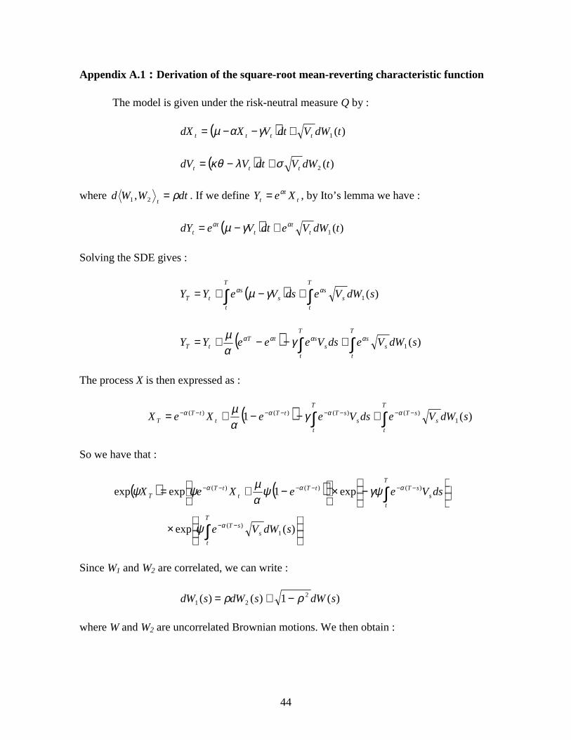
Appendix A.1 : Derivation of the square-root mean-reverting characteristic function
The model is given under the risk-neutral measure Q by :
( ) )(1 tdWVdtVXdX tttt +−−= γαµ
( ) )(2 tdWVdtVdV ttt σλκθ +−=
where dtWWdt
ρ=21, . If we define tt
t XeY α= , by Ito’s lemma we have :
( ) )(1 tdWVedtVedY tt
tt
tαα γµ +−=
Solving the SDE gives :
( )∫ ∫+−+=T
t
T
t
ss
ss
tT sdWVedsVeYY )(1αα γµ
( ) ∫∫ +−−+=T
t
ss
T
t
sstT
tT sdWVedsVeeeYY )(1αααα γ
αµ
The process X is then expressed as :
( ) ∫∫ −−−−−−−− +−−+=T
t
ssT
T
t
ssTtT
ttT
T sdWVedsVeeXeX )(1 1)()()()( αααα γ
αµ
So we have that :
( ) ( )
×
−×
−+=
∫
∫
−−
−−−−−−
T
t
ssT
T
t
ssTtT
ttT
T
sdWVe
dsVeeXeX
)(exp
exp1expexp
1)(
)()()(
α
ααα
ψ
γψψαµψψ
Since W1 and W2 are correlated, we can write :
)(1)()( 221 sdWsdWsdW ρρ −+=
where W and W2 are uncorrelated Brownian motions. We then obtain :

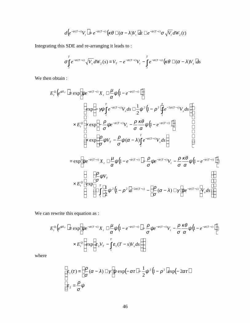
45
( ) ( )
−×
×
−
×
−+=
∫
∫∫
−−
−−−−
−−−−
T
t
ssT
T
t
ssT
T
t
ssT
Qt
tTt
tTXQt
sdWVe
sdWVedsVe
E
eXeeE T
)(1exp
)(expexp
1exp
)(2
2)()(
)()(
α
αα
ααψ
ρψ
ρψγψ
ψαµψ
( )
( )
≤≤
−×
×
−
×
−+=
ℑ∫
∫∫
−−
−−−−
−−−−
TstsWsdWVeE
sdWVedsVe
E
eXe
T
t
ssTQ
T
t
ssT
T
t
ssT
Qt
tTt
tT
;)()(1exp
)(expexp
1exp
2)(2
2)()(
)()(
α
αα
αα
ρψ
ρψγψ
ψαµψ
Since W and W2 are independent,( ) ( ) TsTs sWsW ≤≤≤≤ ℑ⊥ 020 )()( , the equation becomes :
( ) ( )
−×
×
−
×
−+=
∫
∫∫
−−
−−−−
−−−−
T
t
ssTQ
T
t
ssT
T
t
ssT
Qt
tTt
tTXQt
sdWVeE
sdWVedsVe
E
eXeeE T
)(1exp
)(expexp
1exp
)(2
2)()(
)()(
α
αα
ααψ
ρψ
ρψγψ
ψαµψ
( )
( )
×
−+−
×
−+=
∫
∫∫
−−
−−−−
−−−−
T
t
ssT
T
t
ssT
T
t
ssT
Qt
tTt
tT
sdWVe
dsVedsVe
E
eXe
)(exp
12
1exp
1exp
2)(
)(222)(
)()(
α
αα
αα
ρψ
ρψγψ
ψαµψ
At this stage, we did not need the particular square-root specification of the volatility
diffusion. These equations will be also valid for the Ornstein-Uhlenbeck volatility diffusion.
For the square-root model, by Ito’s lemma we can write for the squared volatility :
46
( ) ( ) )()( 2)()()( tdWVedtVeVed t
tTt
tTt
tT σλακθ ααα −−−−−− +−+=
Integrating this SDE and re-arranging it leads to :
( )∫∫ −+−−= −−−−−−T
t
ssT
ttT
T
T
t
ssT dsVeVeVsdWVe )()( )()(
2)( λακθσ ααα
We then obtain :
( ) ( )
( )
( )
−−×
−−−×
−+−
×
−+=
∫
∫∫
−−
−−−−
−−−−
−−−−
T
t
stT
T
tTt
tT
T
t
ssT
T
t
ssT
Qt
tTt
tTXQt
dsVeV
eVe
dsVedsVe
E
eXeeE T
)(
)()(
)(222)(
)()(
)(exp
1exp
12
1exp
1exp
α
αα
αα
ααψ
λαψσρψ
σρ
ψακθ
σρψ
σρ
ρψγψ
ψαµψ
( ) ( )
( )
+−−−+
×
−−−−+=
∫ −−−−
−−−−−−−−
T
t
ssTsT
T
Qt
tTt
tTtTt
tT
dsVee
V
E
eVeeXe
)()(222
)()()()(
)(12
1exp
11exp
αα
αααα
ψγλασρρψ
ψσρ
ψακθ
σρψ
σρψ
αµψ
We can rewrite this equation as :
( ) ( ) ( )
−−×
−−−−+=
∫
−−−−−−−−
T
t
sTQt
tTt
tTtTt
tTXQt
dsVsTVE
eVeeXeeE T
)(exp
11exp
12
)()()()(
εε
ψακθ
σρψ
σρψ
αµψ ααααψ
where
( ) ( ) ( )
=
−−−−
+−=
ψσρε
ατρψατψγλασρτε
2
221 2exp1
2
1exp)()(
47
Define the function ),( VtF by :
{ }
−−= ∫T
t
sTQVt dsVsTVEVtF )(expexp),( 12, εε
then by Feynman-Kac theorem, we have that ),( VtF must satisfy the following PDE :
( )
( )
=
=−−∂∂−+
∂∂+
∂∂
VVTF
FVtTV
FV
V
FV
t
F
2
12
22
exp),(
0)(2
1
ε
ελκθσ
Replacing the time variable t by tT −=τ , we can rewrite this PDE as (without ambiguity,
we keep the same function’s F) :
( )
( )
=
−∂∂−+
∂∂=
∂∂
VVF
FVV
FV
V
FV
F
2
12
22
exp),0(
)(2
1
ε
τελκθστ
If we assume that ),( VF τ is log-linear and given by :
[ ])()(exp),( τττ CVDVF +=
where
0)0(;)0( 2 == CD ε
we have :
[ ]
×=∂∂
×=∂∂
×+=∂∂
),()(
),()(
),()(')('
2
2
2
VFDV
F
VFDV
F
VFCVDF
ττ
ττ
ττττ

48
The PDE for ),( VF τ becomes :
)()()()(2
1)(')(' 1
22 τετλκθτσττ VDVVDCVD −−+=+
After re-arranging it as a polynomial of V , we deduce the ODEs satisfied by )(τD :
==
=++−
ψσρε
τετλτστ
2
122
)0(
0)()()(2
1)('
D
DDD
and by )(τC :
=
=−
0)0(
0)()('
C
DC τκθτ
The actualized characteristic function is then given by :
( )
( ) ( )[ ]);();(exp
11exp
exp)(exp)(
)()()()()(
ψψ
ψακθ
σρψ
σρψ
αµψ
ψψ
αααα
tTCVtTD
eVeeXee
XdssrEf
t
tTt
tTtTt
tTtTr
T
T
t
Qt
−+−×
−−−−+×=
∫−≡
−−−−−−−−−−
49
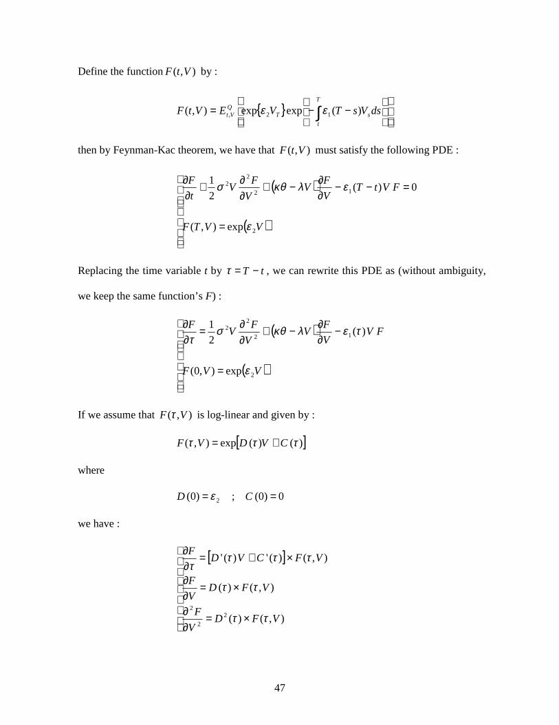
Appendix A.2 : Exact resolution of the ODEs satisfied by D and C in the square-root
framework
The ODEs satisfied by the functions D and C are :
=
=++−
ψσρ
τετλτστ
)0(
0)()()(2
1)(' 1
22
D
DDD
and
=
=−
0)0(
0)()('
C
DC τκθτ
Making the traditional (for Riccati-type ODEs) following transformation :
−= ∫ dssDU )(
2exp)(
2στ
leads to the following linear homogeneous second-order ODE :
0)()(2
1)(')('' 1
2 =−+ τετστλτ UUU
Under this transformation we recover the original functions D and C simply by :
( )
−=
−=
)(ln2
)(
)(
)('2)(
2
2
τσκθτ
ττ
στ
UC
U
UD
A further substitution ( ) )()exp()( τατ UVzV ≡−≡ reduces the ODE to :
0)()(2
1)(')()('' 1
222 =−−+ zezVVzzVz στλααα

50
where )()( 11 τε≡ze . We then only need to solve for the function V(z). Softwares like
Maple® give the solution to this ODE in terms of special functions known as the Whittaker
functions. These functions are related to the well-known confluent hypergeometric
function (see Abramowitz and Stegun, 1968). The solution U is given by :
( ) ( ) ),,(exp),,(exp
)()(ατατ
ατ
ψατψαττ
−−
−
−+−=
≡ecbaWdBecbaMdA
eVU
where M(.) and W(.) are respectively the WhittakerM and the WhittakerW functions and :
−=−
=
=−
−+−=
ααλ
αρσ
αλ
ρα
ρλγσρα
2;
1
2;
12
2
2
dc
ba
Constants A and B are determined by writing down that ψσρ=)0(D and 0)0( =C .

51
Appendix B.1 : Derivation of the Ornstein-Uhlenbeck mean-reverting characteristic
function
The model is given under the risk-neutral measure Q by :
( ) )(12 tdWdtXdX tttt σγσαµ +−−=
( ) )(2 tdWdtd tt βλσκθσ +−=
where dtWWdt
ρ=21, .
From Appendix A.1, we can write the characteristic function as :
( ) ( )
( )
×
−+−
×
−+=
∫
∫∫
−−
−−−−
−−−−
T
t
ssT
T
t
ssT
T
t
ssT
Qt
tTt
tTXQt
sdWe
dsedse
E
eXeeE T
)(exp
12
1exp
1exp
2)(
2)(2222)(
)()(
σρψ
σρψσγψ
ψαµψ
α
αα
ααψ
For the Ornstein-Uhlenbeck model, we can solve for the volatility :
dsedsedesdWe ssT
ssT
sssT
ssT 2)()()(
2)( )( σ
βλσ
βκθσ
βσ
σ αααα −−−−−−−− +−=
Integrating this SDE and re-arranging it leads to :
∫∫∫∫ −−−−−−−− +−=T
t
ssT
T
t
ssT
T
t
sssT
T
t
ssT dsedsedesdWe 2)()()(
2)( 1
)( σβλσ
βκθσσ
βσ αααα
By Ito’s lemma, we also have :
( ) dsededseed sTss
sTs
sTs
sT )(2)(2)(2)( 2 −−−−−−−− ++= αααα βσσσασ
[ ] ( ))(2)(2)(2)( 1222
11 tTT
t
ssT
ttT
T
T
t
sssT edseede −−−−−−−− −−−−= ∫∫ αααα
αβσ
βασσ
βσσ
β
and
52
[ ] ( )
∫∫
∫∫
−−−−
−−−−−−−−
+−
−−−−=
T
t
ssT
T
t
ssT
tTT
t
ssT
ttT
T
T
t
ssT
dsedse
edseesdWe
2)()(
)(2)(2)(22
)( 1222
1)(
σβλρψσψ
βρκθ
αβσ
βασσ
βρψσρψ
αα
αααα
[ ]
( ) ∫
∫−−−−
−−−−
−−−
−+−=
T
t
ssTtT
T
t
ssT
ttT
T
dsee
dsee
σψβ
ρκθψα
ρβ
σαλψβρσσψ
βρ
αα
αα
)()(
2)(2)(2
12
22
The characteristic function is then given by :
( ) ( ) ( )
( )
+
−−−+
−
×
−−−−+=
∫
∫
−−−−
−−
−−−−−−−−
T
t
ssTsT
T
t
ssT
T
Qt
tTt
tTtTt
tTXQt
dsee
dse
E
eeeXeeE T
2)()(222
)(2
)(2)()()(
21
2
1
2exp
122
1exp
σψγλαβρρψ
σψβ
ρκθψσβρ
ψα
ρβσψβρψ
αµψ
αα
α
ααααψ
We can rewrite this equation as :
( ) ( ) ( )
−−−−×
−−−−+=
∫∫
−−−−−−−−
T
t
s
T
t
sTQt
tTt
tTtTt
tTXQt
dssTdssTE
eeeXeeE T
212
23
)(2)()()(
)()(exp
122
1exp
σησηση
ψα
ρβσψβρψ
αµψ ααααψ
where
( ) ( ) ( )
( )
=
−=
−−−−
+−=
ψβρη
ατψβ
ρκθτη
ατρψατψγβρλ
βαρτη
2
exp)(
2exp12
1exp
2)(
3
2
221
53
Define the function ),( σtG as :
−−−−= ∫∫
T
t
s
T
t
sTQt dssTdssTEtG 2
122
3 )()(exp),( σησησησ
By Feynman-Kac theorem, we have that ),( vtG must satisfy the following PDE :
( ) ( )
( )
=
=−+−−∂∂−+
∂∂+
∂∂
23
22
12
22
exp),(
0)()(2
1
σησ
σησησ
λσκθσ
β
TG
GtTtTGG
t
G
Replacing the time variable t by tT −=τ as before, we can rewrite this PDE as (without
ambiguity, we keep the same function’s G) :
( ) ( )
( )
=
+−∂∂−+
∂∂=
∂∂
23
22
12
22
exp),0(
)()(2
1
σησ
στηστησ
λσκθσ
βτ
G
GGGG
Assuming that ),( στG is log-linear and given by :
++= )()()(2
1exp),( 2 τστστστ CDEG
where
0)0(;0)0(;2)0( 3 === CDE η
leads to :
[ ]
[ ]
×++×=∂∂
×+=∂∂
×
++=
∂∂
),()()(),()(
),()()(
),()(')(')('2
1
2
2
2
2
σττστσττσ
σττστσ
σττστσττ
GDEGEG
GDEG
GCDEG
54
The PDE satisfied by ),( στG becomes :
( )[ ]
( )[ ]
[ ]212
222
)()(
)()(
)()()(2
1)(')(')('
2
1
στηστη
τστλσκθ
τσττβτστστ
+−
+−+
++=++
DE
DEECDE
After re-arranging it as a polynomial of σ, we deduce the ODEs satisfied by )(τE :
==
=++−
ψβρη
τητλτβτ
3
122
2)0(
0)()()(2
1)('
2
1
E
EEE
by )(τD :
=
=+−+−
0)0(
0)()()()()()(' 22
D
EDDED τητκθτλττβτ
and by )(τC :
=
=−−−
0)0(
0)()(2
1)(
2
1)(' 222
C
DDEC τκθτβτβτ
The actualized characteristic function is then given by :
( )
( ) ( )
−+−+−×
−−−−+=
∫−≡
−−−−−−−−−−
);();();(2
1exp
122
1exp
exp)(exp)(
2
)(2)()()()(
ψσψσψ
ψα
ρβσψβρψ
αµψ
ψψ
αααα
tTCtTDtTE
eeeXee
XdssrEf
tt
tTt
tTtTt
tTtTr
T
T
t
Qt
55
Appendix B.2 : Exact resolution of the ODE satisfied by E in the Ornstein-Uhlenbeck
framework
The ODEs satisfied by the functions E is :
==
=++−
ψβρη
τητλτβτ
3
122
2)0(
0)()()(2
1)('
2
1
E
EEE
As detailed in Appendix A.2, we use two transformations before getting the exact solution
E. Making the first transformation :
−= ∫ dssEU )(exp)( 2βτ
and the further substitution ( ) )()exp()( τατ UVzV ≡−≡ lead to :
( ) ( ) ),,(exp),,(exp
)()(ατατ
ατ
ψατψαττ
−−
−
−+−=
≡
ecbaWdBecbaMdA
eVU
where again M(.) and W(.) are respectively the WhittakerM and the WhittakerW functions
and :
−=−
=
=−
−+−=
ααλ
αρβ
αλ
ραρλγβρα
2
2;
12
;12
22
2
2
dc
ba
Constants A and B are determined by writing down that 1)0( =U and βρψ−=)0('U . We
recover the function E by :
)(
)('1)(
2 ττ
βτ
U
UE −=

56
To see that neither D (nor C) could be expressed in a closed-form way, we use a traditional
technique to solve linear first-degree ODEs to find :
( )
−+−= ∫ −
τλαλτ
λτ ρβψλττβ
κθτ0
2)()(1
)(
1)( dssUeeUe
UeD ss
This expression could not be simplified further.
57
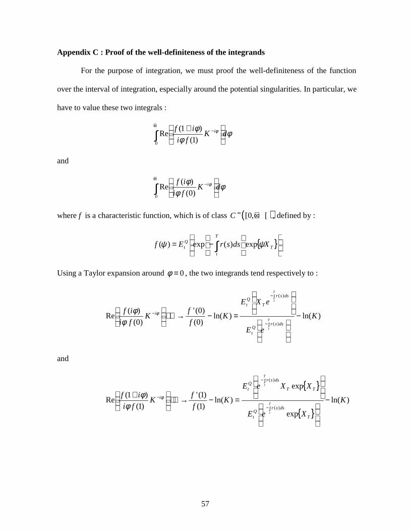
Appendix C : Proof of the well-definiteness of the integrands
For the purpose of integration, we must proof the well-definiteness of the function
over the interval of integration, especially around the potential singularities. In particular, we
have to value these two integrals :
φφ
φ φ dKfi
if i∫+∞
−
+
0 )1(
)1(Re
and
φφ
φ φ dKfi
if i∫+∞
−
0 )0(
)(Re
where f is a characteristic function, which is of class ( )[,0[ +∞∞C , defined by :
{ }
−= ∫ T
T
t
Qt XdssrEf ψψ exp)(exp)(
Using a Taylor expansion around 0=φ , the two integrands tend respectively to :
)ln()ln()0(
)0('
)0(
)(Re
)(
)(
K
eE
eXE
Kf
fK
fi
ifT
t
T
t
dssrQt
dssr
TQt
i −
=−→
∫−
∫−
− φ
φφ
and
{ }
{ })ln(
exp
exp
)ln()1(
)1('
)1(
)1(Re
)(
)(
K
XeE
XXeE
Kf
fK
fi
if
T
dssrQt
TT
dssrQt
iT
t
T
t
−
=−→
+∫−
∫−
− φ
φφ

58
Appendix D : Feynman-Kac theorem (Karatzas and Shreve 1991)
Under some regularity assumptions, if we suppose that ddTVtF ℜ→ℜ×],0[:),(
is of class ( )dTC ℜ×],0[2,1 and satisfies the Cauchy problem :
=
=−++∂∂
)(),(
0),(),(),(
VkVtF
VtFVthVtgFAt
Ft
where At is the second order differential operator, then ),( VtF is unique and admits the
stochastic representation :
−+
−
=
∫ ∫
∫T
t t
s
T
t
sT
Vt
ddsVshVg
dsVshVk
EVtF
τττ
τ ),(exp),(
),(exp)(
),( ,

59
Appendix E : Derivation of the Greeks
Recall that the Call premium is given by :
( ) ( ))ln()0;,()ln()1;,(),( ,2
,1 KXQKTtfKXQTtfTtCall T
TtT
Tt >−>=
For simplicity, we denote );,( ψTtf by )(ψf and ( ))ln(, KXQ TTt
j > by jQ . We need to
compute the following derivatives :
)()( )( ψψψ α fe
X
f tT
t
−−=∂
∂
( ))1(
)(1
)1(
)(
)(
f
fe
X
f
f
tT
t
ψψ
ψ
α −−−=∂
∂
∫+∞
−−−
+=∂∂
0
)(1
)1(
)1(Re φφ
πφ
α
dKf
ife
X
Q itT
t
∫+∞
−−−
=
∂∂
0
)(2
)0(
)(Re φφ
πφ
α
dKf
ife
X
Q itT
t
We then can write :
∂∂
−∂∂
+∂∂=
∂∂=
∂∂≡
−
−
ttt
X
t
X
X
X
QKf
X
QfQ
X
fe
X
TtCalle
e
TtCallTtDelta
t
t
t
211 )0()1(
)1(
),(
),(),(
By a “formal” change of variable, we can show that :
tt X
QKf
X
Qf
∂∂
=∂∂ 21 )0()1(
and we can deduce the formula for the Delta as given in the main text.

60
Define the Gamma by :
tXe
TtDeltaTtGamma
∂∂≡ ),(
),(
Using the same calculus done to derive the Delta leads to :
( ) ( )∫∞+
−−−−
−−−
−−−
−−−−−−
−
−
++−=
∂∂
+
∂∂+−
=
∂∂=
0
2)(2)(
1)(
1)(
1)(
)1(Re),(1
)1(
)1()1(
),(),(
φφπ
φα
α
α
αα
dKifee
TtDeltaee
X
Qfee
QX
feeQfee
e
X
TtDeltaeTtGamma
iXtT
XtT
t
XtT
t
XtTXtT
X
t
X
t
t
t
tt
t
t
For the Vega, consider first the square-root model :
tV
TtCallTtVega
∂∂≡ ),(
),(
We compute the following derivatives :
)();()( )( ψψ
σρψψ α fetTD
V
f tT
t
−−=
∂∂ −−
( ))1(
)(1)1;();(
)1(
)(
)(
f
fetTDtTD
V
f
f
tT
t
ψψσρψ
ψ
α
−−−−−=
∂
∂
−−
∫+∞
−−−
+
−
−−+−=
∂∂
0
)(1
)1(
)1()1;()1;(Re
1 φφσρ
φφ
πφα dK
f
ife
i
tTDitTD
V
Q itT
t
∫+∞
−−−
−
−=
∂∂
0
)(2
)0(
)();(Re
1 φφσρ
φφ
πφα dK
f
ife
i
itTD
V
Q itT
t

61
We now can write for the Vega :
ttt V
QKf
V
QfQ
V
fTtVega
∂∂
−∂∂
+∂
∂= 211 )0()1(
)1(),(
∫
∫∞+
−
∞+−
−−
−−
+
−−+−+
−−=
0
0
1)(
)();(
Re
)1()1;()1;(
Re1
)1()1;(
φφφ
φπ
φφφ
φπ
σρ
φ
φ
α
dKifi
itTDK
dKifi
tTDitTD
QfetTD
i
i
tT
For the Ornstein-Uhlenbeck model, define the Vega by :
t
TtCallTtVega
σ∂∂≡ ),(
),(
The following derivatives are needed :
)();();()( )( ψψ
βρψσψ
σψ α fetTDtTE
f tTt
t
−−+−=
∂∂ −−
[ ]( ) )1(
)(1
)1;();()1;();()1(
)(
)( f
fe
tTDtTDtTEtTEf
f
ttT
t
t
ψσψ
βρ
ψσψ
σ
ψ
α
−−
−−−+−−−=
∂
∂
−−
∫∞+
−
−−
+
−−−+−
+
−−+−
=∂∂
0 )(
1
)1(
)1(
)1;()1;(
)1;()1;(
Re1 φφ
βρ
φφ
σφ
φ
πφ
α
dKf
if
ei
tTDitTD
i
tTEitTE
V
Q i
tT
t
t
∫+∞
−−−
−
−+
−=
∂∂
0
)(2
)0(
)();();(Re
1 φφσρ
φφσ
φφ
πφα dK
f
ife
i
itTD
i
itTE
V
Q itTt
t

62
The Vega can be written as :
ttt
QKf
QfQ
fTtVega
σσσ ∂∂
−∂∂
+∂∂= 21
1 )0()1()1(
),(
∫
∫
∞+−
∞+−
−−
−+
−−
+
−−+−+
−−+−
+
−−+−=
0
0
1)(
)();();(
Re
)1()1;()1;(
)1;()1;(
Re1
)1()1;()1;(
φφφ
φσφ
φπ
φφ
φφ
σφ
φ
π
σβρσ
φ
φ
α
dKifi
itTD
i
itTEK
dKif
i
tTDitTD
i
tTEitTE
QfetTDtTE
it
i
t
ttT
t
63
Footnotes
* Ph.D. candidate in Finance at the École HEC Montréal. Financial support was provided by
the Risk Management Chair, the FCAR and the Social Sciences and Humanities Research
Council of Canada. I would like to thank my professors, Georges Dionne, Jean-Guy
Simonato and Peter Christoffersen for their comments. I am also grateful to the participants
at the “Brown Bag” seminar at HEC Montréal, at the 2nd CIRPÉE annual conference at
Montreal and at the QMF 2002 conference at Sydney for helpful discussions.