Construction of Gauss-Christ of fei Quadrature Formulas · 2012-05-01 · Construction of Gauss-Christ of fei Quadrature Formulas By Walter Gautschi* 1. ... are associated with the

Construction of Gauss-Christ of feiQuadrature Formulas

By Walter Gautschi*

1. Introduction. Let w(x) be a given function ("weight function") defined on a

finite or infinite interval (a, b). Consider a sequence of quadrature rules

(1.1) / f(x)w(x)dx = ¿ Xr(n)/fe(n)) , n = 1, 2, 3, • • • .

Each of these rules will be called a Gauss-Christoffel quadrature formula if it has

maximum degree of exactness, i.e. if (1.1) is an exact equality whenever / is a poly-

nomial of degree 2n — 1. It is a well-known fact, due to Christoffel [3], that such

quadrature formulas exist uniquely, provided the weight function w(x) is nonnega-

tive, integrable with /* w(x)dx > 0, and such that all its moments

(1.2) ßk= xkw(x)dx, k = 0,1,2, ■■■ ,Ja

exist. Then, moreover, £r(n) £ (a, b), and Xr(n) > 0. If w(x) is not of constant sign,

Gauss-Christoffel formulas still exist if certain Hankel determinants in the moments

are different from zero [21]. In this case, however, some of the abscissas £rM may

fall outside the interval (a, b) ; in particular, they may become complex. We shall

call £r(n) the Christoffel abscissas, and Xr(n) the Christoffel weights associated with

the weight function w(x).

Gauss [7] originally considered the case w(x) = 1 on [— 1,1]. Other classical cases

are associated with the names of Jacobi, Laguerre, and Hermite. In more recent

times, the subject has experienced a considerable resurgence, as is evidenced by the

appearance of numerous numerical tables [15], [21], both relative to classical and

nonclassical weight functions. The emergence of powerful high-speed computers,

undoubtedly, has been a major force in this development. Curiously enough, the

constructive (algorithmic) aspect of the subject, until very recently, has remained at

the state of development in which it was left by Christoffel, and Stieltjes [20]. The

generally recommended procedure still consists [1] in constructing the system {xr}

of orthogonal polynomials associated with the weight function w(x), and to obtain

£r(n) as the zeros of ir„, and Xr(n), in a number of possible ways, in terms of these

orthogonal polynomials. An alternative procedure, suggested by Rutishauser [19],

makes use of the quotient-difference algorithm, while Golub and Welsch [11] use

Francis' QÄ-transformations to compute £r(n) as eigenvalues of a Jacobi matrix

and Xr(n) as the first component of the corresponding eigenvectors. These methods,

as interesting as they are, appear to be computationally feasible, for large n, only

if the orthogonal polynomials xr, or the associated Stieltjes continued fraction, are

explicitly known. Otherwise, they are subject to severe numerical instability,

Received September 11, 1967.* This work was performed in part at the Argonne National Laboratory, Argonne, Illinois,

under the auspices of the U. S. Atomic Energy Commission.

251License or copyright restrictions may apply to redistribution; see https://www.ams.org/journal-terms-of-use

252 WALTER GAUTSCHI

making it virtually impossible to obtain meaningful answers, unless one resorts to

multiple-precision work.

The reason for this is the ill-conditioned character of the problem which these

methods attempt to solve. The problem, basically, is the purely algebraic one of

deriving £r(n>, Xr(?l) from the first 2n moments of w(x), i.e. of solving the algebraic

system of equations

(1.3) Èx,wK,wf-/i» (fc = 0, 1,2, ...,2n-l).r=l

It will be shown (Section 2) that for a finite interval (0, 1) the (asymptotic, relative)

condition number k„ for this problem can be estimated from below by

(1.4) Kn > min U, — ) max {(1 + {«) fl L l)+ **'t> ) Í "

Considering that the abscissas £r(n), for large n, tend to cluster near the endpoints

of the interval (0, 1), many of the differences £r(n) — &(n) will be quite small in abso-

lute value. Consequently, some of the products in (1.4), and thus the lower bound

for Kn, are likely to be very large when n is large.

To give a more concrete idea of just how large k„ may become, we note [22, p.

309] that for a wide class of weight functions the abscissas £r(n) ultimately (as n

—> =o ) assume an arc cos-distribution, i.e.

(1.5) £r(n) = i(l + cos e/n)) , e/n) = (2r - l)x/2n .

Replacing the £rCn) in (1.4) by their approximate values in (1.5), one finds that

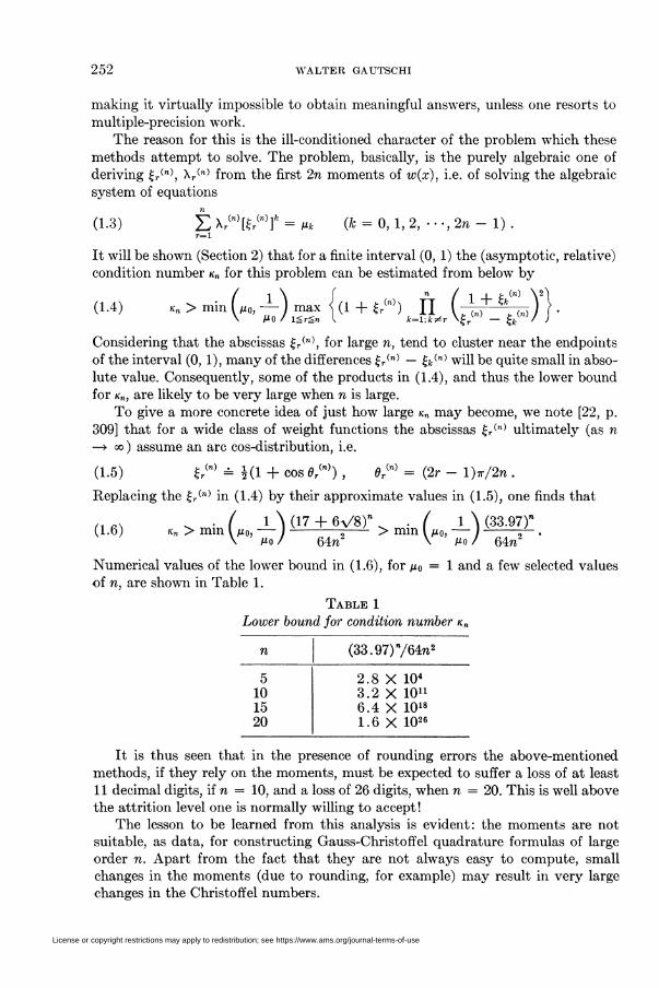
,,. ^ . ( 1 \ (17 + 6V8)" . . / 1 \ (33.97)"(1.6) Kn > mm I /to, — J-—:—- > min I /t0, ■— ) nÁ / .

V mo/ 64n \ /to/ 64w

Numerical values of the lower bound in (1.6), for /t0 = 1 and a few selected values

of n, are shown in Table 1.

Table 1

Lower bound for condition number k„

5101520

(33.97)n/64n2

2.8 X 1043.2 X 10u

6.4 X 10181.6 X 1026

It is thus seen that in the presence of rounding errors the above-mentioned

methods, if they rely on the moments, must be expected to suffer a loss of at least

11 decimal digits, if n = 10, and a loss of 26 digits, when n = 20. This is well above

the attrition level one is normally willing to accept!

The lesson to be learned from this analysis is evident: the moments are not

suitable, as data, for constructing Gauss-Christoffel quadrature formulas of large

order n. Apart from the fact that they are not always easy to compute, small

changes in the moments (due to rounding, for example) may result in very large

changes in the Christoffel numbers.

License or copyright restrictions may apply to redistribution; see https://www.ams.org/journal-terms-of-use

GAUSS-CHRISTOFFEL QUADRATURE FORMULAS 253

In Section 3 we propose an alternative procedure for generating Gauss-Christoffel

formulas, which is based on a suitable discretization of the inner product (/, g) =

¡lf(x)g(x)w(x)dx, and thus bypasses the moments altogether. As the discretization

is made infinitely fine, the process converges to the desired Christoffel numbers pro-

vided the singularities of w(x), if any, are located at the endpoints of the interval

and are monotonie. Extensive tests have shown that the method is reasonably

accurate, relatively "inexpensive," and requiring only single-precision arithmetic.

A computer algorithm (in ALGOL) is to appear in [10].

Cases may arise in which our method converges very slowly. While approximate

Christoffel numbers are still obtained, it may be desirable to further improve

their accuracy. This can be done by applying Newton's method to a system of equa-

tions, equivalent to (1.3), using as initial approximations the approximate Christoffel

numbers already obtained. An appropriate procedure for this will be described in

Section 4. Unfortunately, this iterative refinement calls for the moments of the

weight function, and therefore is of limited practical value, unless one is prepared

to use higher-precision work in some preliminary parts of the computation.

The ability to generate Gauss-Christoffel quadrature formulas, as needed, is of

considerable practical interest, not only for integrating singular functions, but also

for the numerical solution of integral equations and boundary value problems. We

also remark that this new capability may well be useful in future systems of "auto-

mated numerical analysis," such as the NAPSS system currently under development

at Purdue University [18].

In the appendix are collected a few general properties, more or less known, of

orthogonal polynomials which are relevant to our discussion in Sections 3, 4.

Extensions of our work seem possible to quadrature formulas of maximum de-

gree of exactness, where some of the abscissas are prescribed, or the quadrature

sum involves derivative values as well as function values. Such generalizations,

however, will not be considered here.

2. Condition of the Classical Approach. In this section we discuss the con-

dition of the problem of solving the system of algebraic equations (1.3). In particular

we derive the estimates (1.4) and (1.6) for the asymptotic condition number, and

compare them with the condition of inverting Hilbert matrices.

It will be useful, first, to consider the condition of a mapping M, say, from one

normed space X into another, F:

M : X-^Y.

Following Rice [17], we define the (relative) 5-condition number k(8) of M at xo £ X

by

(2.1) «Wtfm^ll^' + ^-^'ll/A.v w lUII-a ||Mzo|| / Hzoll

Thus, k(ô) represents the maximum amount by which a (relative) perturbation in

the space X, as given by 5/1 Wl, is magnified under the mapping M. Since the

perturbations to be considered are small (rounding errors!) it is natural to consider

the (relative) asymptotic condition number k of M at xo, as defined by


254 WALTER GAUTSCHI

(2.2) K = lim k(S) ,

where the existence of the limit, of course, is assumed.

In solving the system of equations (1.3) we are dealing with the mapping M:

X —» F of a 2n-dimensional Euclidean space into itself, if we identify X with the

"moment space," and Y with the space of Christoffel numbers. This mapping is

one-to-one in the neighborhood of the exact solution of (1.3). We may write (1.3)

in the compact form

(2.3)

where xT

F2n), and

(ßo, Ml,

F(y) = x,

-, /t2n-i), yT = (Xl, • • -, X„, £l, •, £,), F* - (Fh Ft,

(2.4) Fk(y) = Z X^*"1 (k = 1, 2, 2n) .

The (relative) asymptotic condition number k = kk for solving the nonlinear

system of equations (2.3) at x<¡ is well known to be (cf. [17])

(2.5) IËsJJ\yo\\

It^ö/o)]"1!!,

where y0 is the solution of F(y) = x0, and ^(2/) denotes the Jacobian matrix of F.

The matrix norm in (2.5) is assumed to be subordinate to the vector norm chosen

in X and Y. From (2.4) we obtain by a simple computation that

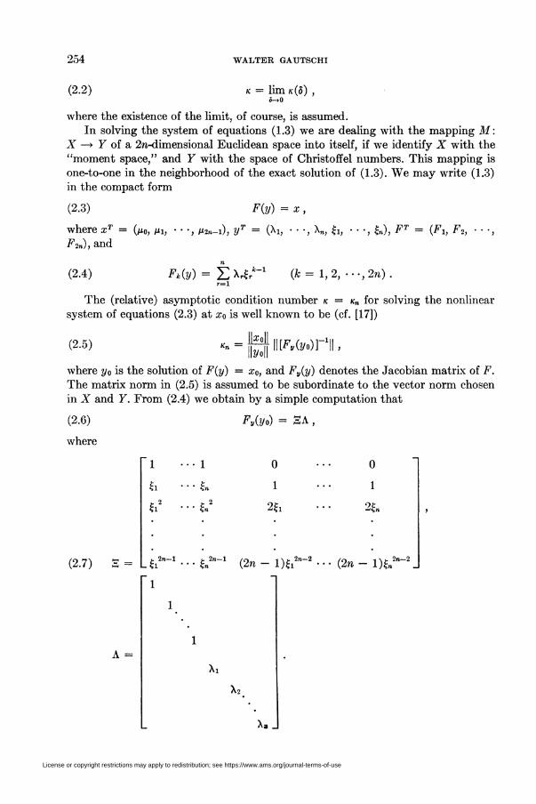
(2.6)

where

Ft(y0) = HA,

(2.7) S

1

£1

íi

1

c ain

0

1

2?,

$„ (2n — l)?i

0

1

2?„

(2n - l)?„2i

A =

X8



(For simplicity, we have written |r for £r(n), and Xr for \rM.) Hence, by (2.5),

C2 8) k = JJ^îli IIa^w-1!!W Kn ||2/o|| ||A „ || .

We now choose our norms. We take as vector norm ||a;|| = maxs \xk\, and corre-

spondingly as matrix norm ||.4|| = max* ^r |<z&rJ. We further assume the basic

interval to be (0, 1), and w(x) ^ 0. Clearly, ||a;o|| i5 /to- Since Xr > 0, and ^r=i Xr =

/to, we have Xr < /t0. Also, 0 < £r < 1. Therefore,

\\y0\\ = max:(Xr, £r) < max (1, /t0) .r

Moreover, with the matrix norm as defined,

llA-ig-ièminCl, l/ÎIS-1».

It thus follows from (2.8), that

/to min (1, l//to) ||,-î||Kn> max (1,/to) l|A "'

or, equivalently,

(2.9) K„>min(/t0, l/ÎIS-1!!.

Further discussion now hinges on obtaining a lower bound for || E_1||, where S is

the matrix in (2.7), a confluent Vandermonde matrix [8].

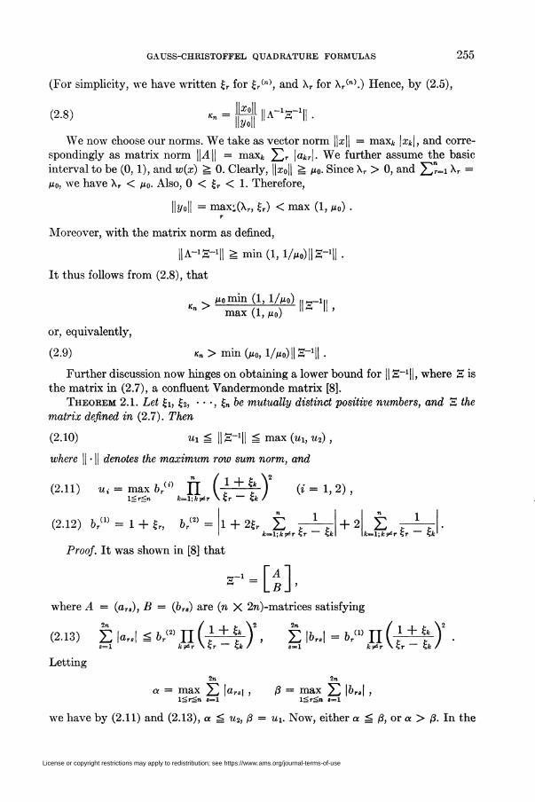
Theorem 2.1. Let £i, £2, • • -, £n be mutually distinct positive numbers, and S the

matrix defined in (2.7). Then

(2.10) Mi g || S"1!! á max (uh u2),

where || • || denotes the maximum row sum norm, and

brU) ft (j^fT(2.11 u,- = max 6rl" L)lgrgn

(2.12) brm = 1 + £r, b/2) = 1 + 2£r ¿ r-i—k~\;k*r Çr ~ Kk

+ 2b—l;*|rfr £r — £*

Proof. It was shown in [8] that

HIwhere A = (ara), B = (brs) are (n X 2n)-matrices satisfying

(2.13) z ia„i ̂ t,« n (t^Y , ë i6«i = &r(i) n (t^t)2 •s=l A:?*)- \ Çr — Kk / s=l *7är \ Kr — « /

Letting

2» 2n

a = max Z la^l > ß — max 2 l&™| ,lárín 8=1 lSr^n 8=1

we have by (2.11) and (2.13), a ^ u2, ß = u\. Now, either a g /3, or a > ß. In the


256 WALTER GAUTSCHI

first case, ||S_1|| = ß = Mi, in the second case, Mi < ||E-1¡| = a ^ u2. Hence, (2.10)

holds in either case, and Theorem 2.1 is proved.

We remark that in the case ui ^ w2 we have || H-1|| = U\.

Applying Theorem 2.1 to (2.9), we obtain

(2.14) Kn > min (/t0, — ) max {(1 + £r) Ü ( \ + \ ) !,

the result already stated in (1.4).

Using the approximations (cf. (1.5))

kr = Kl + Xr) , Xr = COS 0r , 0r = (2f - 1)tt/2« ,

where xr are the zeros of the Chebyshev polynomial Tn(x), we may estimate

(2.15)(i + « n (f^)2 - i (3 +.,,) n (f^)2

i_[ r.(3) ]2 j_ [ r.(3) I22(3 +

We have

sin (n6r)(2.16) Tn'(xr) = 7Y(cos0r) = n v" ry = (-1)'

sin ör sin er

Now the maximum in (2.14) is obviously larger than the respective expression

evaluated for any fixed r = r0. Choosing r0 = [n/2] + 1, we obtain in view of (2.15),

(2.16)

1 . ( 1 \ [cnTn(3)~- mm I /to, — ) -—8 \ mo / L n

k„ >

Mo

c„ = 1 (n odd) ,

c„ = cos (ir/2n) (n even) .*

Since cos (ir/2n) ^ 1/ V 2 (n ^ 2), it follows that cn 5; 1/ V 2, and so

k„ > (l/16n2) min (Mo, l//io)[T„(3)]2 .

As is well known, zn = THi/¿) satisfies

Zn+l — &Zn + Zn-1 = 0 , 20 = 1 , 2l = 3 .

Hence, using standard results from the theory of linear difference equations,

zn = r,(3) = §(ii" + Í2») , ii = 3+V8, i2 = 3 - V8 .

It follows that r„(3) > 5Í1", and we finally obtain

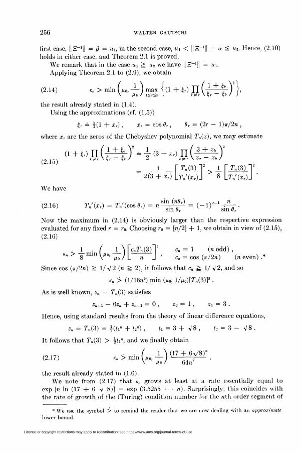
(2.17) k„ > min. ( 1 \ (17 + 6V8)"111 I Mo, - J -——- :

V Mo / 64n

the result already stated in (1.6).

We note from (2.17) that k„ grows at least at a rate essentially equal to

exp [n In (17 + 6 V 8)] = exp (3.5255 • • • n). Surprisingly, this coincides with

the rate of growth of the (Turing) condition number for the nth order segment of

* We use the symbol > to remind the reader that we are now dealing with an approximate

lower bound.



the Hubert matrix, as estimated by Todd [23]. Computing Christoffel numbers on

the interval (0, 1) from given moments is therefore about as ill-conditioned as the

inversion of Hubert matrices!

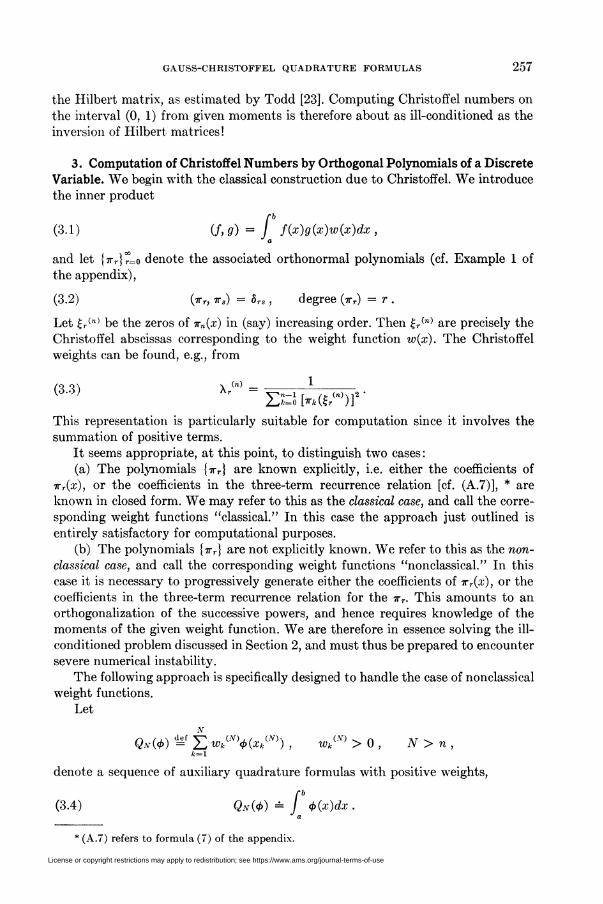
3. Computation of Christoffel Numbers by Orthogonal Polynomials of a Discrete

Variable. We begin with the classical construction due to Christoffel. We introduce

the inner product

(3.1) (f,g) = / f(x)g(x)w(x)dx ,

and let J7rr}r=o denote the associated orthonormal polynomials (cf. Example 1 of

the appendix),

(3.2) (xr, xs) = 5rs, degree (irr) = r .

Let %,M be the zeros of tu(x) in (say) increasing order. Then çV(n) are precisely the

Christoffel abscissas corresponding to the weight function w(x). The Christoffel

weights can be found, e.g., from

Cn)

(3-3) Xr" 'Züb^f'

This representation is particularly suitable for computation since it involves the

summation of positive terms.

It seems appropriate, at this point, to distinguish two cases :

(a) The polynomials ¡xr} are known explicitly, i.e. either the coefficients of

Trr(x), or the coefficients in the three-term recurrence relation [cf. (A.7)], * are

known in closed form. We may refer to this as the classical case, and call the corre-

sponding weight functions "classical." In this case the approach just outlined is

entirely satisfactory for computational purposes.

(b) The polynomials {t?} are not explicitly known. We refer to this as the non-

classical case, and call the corresponding weight functions "nonclassical." In this

case it is necessary to progressively generate either the coefficients of tt(x), or the

coefficients in the three-term recurrence relation for the irr. This amounts to an

orthogonalization of the successive powers, and hence requires knowledge of the

moments of the given weight function. We are therefore in essence solving the ill-

conditioned problem discussed in Section 2, and must thus be prepared to encounter

severe numerical instability.

The following approach is specifically designed to handle the case of nonclassical

weight functions.

Let

Ndef

fc— 1

denote a sequence of auxiliary quadrature formulas with positive weights,

QA4>) = E Wkm<t>(xkm) , Wk(N) > 0 , N>n,A-=l

îence of auxiliary quadrature

(3.4) Qn(<p) = J <j>(x)dx

* (A.7) refers to formula (7) of the appendix.


258 WALTER GAUTSCHI

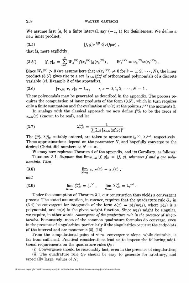
We assume first (a, b) a finite interval, say (—1, 1) for definiteness. We define a

new inner product,

(3.5) [/, g]s = QN(fgw),

that is, more explicitly,

(3.5') If, 9h = E Wkmf(xkm)g(Xkm) , Wkm = Wkmw(xkm) .k=l

Since Wk(N) > 0 (we assume here that w(xkiN)) ^ 0 for k = 1, 2, • • -, N), the inner

product (3.5') gives rise to a set {irr.jv}^1 of orthonormal polynomials of a discrete

variable (cf. Example 2 of the appendix),

(3.6) [wr.N, TTs,n]n = Sts , T, 8 = 0, 1, 2, • • -, N - 1 .

These polynomials may be generated as described in the appendix. The process re-

quires the computation of inner products of the form (3.5'), which in turn requires

only a finite summation and the evaluation of w(x) at the points Xk(JV) (no moments !).

In analogy with the classical approach we now define £("at to be the zeros of

■ïïn,N(x) (known to be real), and let

(n)

(3-7) Kn - Vn_j¿^=0 [TTk.NKÇr.NJi

The Q"N, \^lf, suitably ordered, are taken to approximate £r(n), Xr<n), respectively.

These approximations depend on the parameter N, and hopefully converge to the

desired Christoffel numbers as N —> °o.

We may now rephrase Theorem 4 of the appendix, and its Corollary, as follows :

Theorem 3.1. Suppose that limAf-,,» [/, g]N = (/, g), whenever f and g are poly-

nomials. Then

(3.8) lim 7rr,jv(a;) = irT(x) ,JV-«o

and

(3.9) lim {g, = ç-r(n) , lim \% = Xr(n).N—HX) N—*tX3

Under the assumption of Theorem 3.1, our construction thus yields a convergent

process. The stated assumption, in essence, requires that the quadrature rule Qn in

(3.4) be convergent for integrands of the form <p(x) = p(x)w(x), where p(x) is a

polynomial, and w(x) is the given weight function. Since w(x) might be singular,

we require, in other words, convergence of the quadrature rule in the presence of singu-

larities. Fortunately, most of the common quadrature formulas do converge, even

in the presence of singularities, particularly if the singularities occur at the endpoints

of the interval and are monotonie [5], [16].

From the computational point of view, convergence alone, while desirable, is

far from sufficient. Practical considerations lead us to impose the following addi-

tional requirements on the quadrature rules Qn ■

(i) Convergence should be reasonably fast, even in the presence of singularities ;

(ii) The quadrature rule Qn should be easy to generate for arbitrary, and

especially large, values of N;



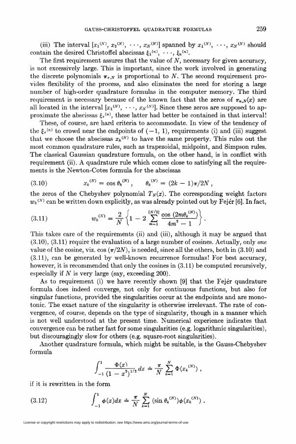
(iii) The interval [xi<-N), x2(JV), • • -, xn(N)] spanned by xi*-N), ■ ■ -, xnÍN) should

contain the desired Christoffel abscissas £i(k), • • -, £>»(n)-

The first requirement assures that the value of JV, necessary for given accuracy,

is not excessively large. This is important, since the work involved in generating

the discrete polynomials ttt,n is proportional to N. The second requirement pro-

vides flexibility of the process, and also eliminates the need for storing a large

number of high-order quadrature formulas in the computer memory. The third

requirement is necessary because of the known fact that the zeros of irn¡N(x) are

all located in the interval [xi(N), • • -, xn(n)]- Since these zeros are supposed to ap-

proximate the abscissas £r<n), these latter had better be contained in that interval!

These, of course, are hard criteria to accommodate. In view of the tendency of

the £r(n) to crowd near the endpoints of ( — 1, 1), requirements (i) and (iii) suggest

that we choose the abscissas Xk^m to have the same property. This rules out the

most common quadrature rules, such as trapezoidal, midpoint, and Simpson rules.

The classical Gaussian quadrature formula, on the other hand, is in conflict with

requirement (ii). A quadrature rule which comes close to satisfying all the require-

ments is the Newton-Cotes formula for the abscissas

(3.10) xkm = cos dkm , 6km = (2k - l)r/22V ,

the zeros of the Chebyshev polynomial Tn(x). The corresponding weight factors

Wk(tf) can be written down explicitly, as was already pointed out by Fejér [6]. In fact,

lN/2] cos (2mekm)(3.11) »"-ffl-íl- ï

J» L m=i 4¿m

This takes care of the requirements (ii) and (iii), although it may be argued that

(3.10), (3.11) require the evaluation of a large number of cosines. Actually, only one

value of the cosine, viz. cos (ir/2N), is needed, since all the others, both in (3.10) and

(3.11), can be generated by well-known recurrence formulas! For best accuracy,

however, it is recommended that only the cosines in (3.11) be computed recursively,

especially if N is very large (say, exceeding 200).

As to requirement (i) we have recently shown [9] that the Fejér quadrature

formula does indeed converge, not only for continuous functions, but also for

singular functions, provided the singularities occur at the endpoints and are mono-

tonic. The exact nature of the singularity is otherwise irrelevant. The rate of con-

vergence, of course, depends on the type of singularity, though in a manner which

is not well understood at the present time. Numerical experience indicates that

convergence can be rather fast for some singularities (e.g. logarithmic singularities),

but discouragingly slow for others (e.g. square-root singularities).

Another quadrature formula, which might be suitable, is the Gauss-Chebyshev

formula

L^$f2dx^fÈiHxkm)'

form

(3.12) P <b(x)dx = -— £ (sin ekm)<t>(xkm) .J -1 iv ,t=i

(1-

if it is rewritten in the form


260 WALTER GAUTSCHI

Here we have exact equality if <p(x) = p2N-i(x)(l — x2)~112, where p2N-i(x) is a poly-

nomial of degree 2N — 1. The formula (3.12) is therefore particularly suitable in

cases where the weight function w(x) has square-root singularities at the endpoints

±1, which is one of the cases where the Fejér formula converges very slowly.

It is interesting to point out the close kinship between the Fejér formula (3.10),

(3.11) and the Gauss-Chebyshev formula (3.12), noting that the right-hand side in

(3.11) is nothing else but the truncated Fourier expansion of (t/N) sin 0it('v), the

weight factor in (3.12)!

We may also remark, at this point, that in the process of generating the poly-

nomials iTr.N (r = 0, 1, • • -, n), one needs to evaluate inner products [/, g]x only for

polynomials /, g of degree ¿n. Using the Fejér quadrature formula, which is of

interpolatory type, it thus follows from (3.1), (3.5) that for such/ and g, [f, g]N =

(/, g) whenever w(x) is a polynomial of degree m, and N > 2n + m. As a result, our

process of constructing Christoffel numbers, based on the Fejér formula (3.10), (3.11),

is exact if w(x) is a polynomial of degree m and N > 2n + m. The process, in this

case, converges trivially. Similarly, our process of constructing Christoffel numbers,

based on the Gauss-Chebyshev formula (3.12), is exact if w(x) — (1 — x2)~l!2 and N

> n.

Our development so far assumed [—1, 1] as the basic interval. This is no re-

striction of generality. In fact, the case of an arbitrary finite interval [a, b] is readily

reduced to the case considered by a linear transformation of the independent vari-

able. In the case of a half-infinite interval, say (0, go), let <p(t) be any continuously

differentiable monotonically increasing function mapping the interval ( — 1, 1) onto

(0, » ). Then

(f,g) = J f(x)g(x)w(x)dx = J /(*(¿))ff(*(i))w(*(0)*'(0d<,

and we can proceed as before if we define

[f,gh = iwkmf(cp(xkm))g(<p(xkm)),A:^l

where now

Wkm = w^N)w((b(xkm))<p'(xkm) .

An analogous device applies for a doubly infinite interval (— eo, °o), in which case

<p(t) is to map (—1, 1) onto (—=°, go). Simple transformation functions, which

proved satisfactory, are <p(t) = (1 + t)/(l — t) for (0, «), and <p(t) = t/(l — t2) for

(-co, oo).

We conclude this section with a few comments on the computation of the

zeros £^ of irn,N(x). We assume that the coefficients ar, br+i in the recurrence

relation (cf. (A.7*))

irr+l,N(x) = ((X — ar)irr,N(x) — br1Tr-l,N(x))/br+l

(3.13) (r = 0, 1, ...,n-l),

ito,n(x) = [1, 1]aTx 2, t-i,n(x) = 0 ,

have already been obtained by the methods described in the appendix. We propose

two different procedures to find the Christoffel abscissas, depending on whether the



|rw) are desired for ail k = 1, 2, • • -, n, r = 1, 2, • ■ -, k, or £r(,l), r = 1, 2, • • -, n,

are desired for only one, or a few selected values of n.

In the first case we apply Newton's method to each of the equations Tk,N(x)

= 0 (fc = 2, 3, • • -, n), using (£^7° + £r0c~1'')/2 as initial approximation for £rlk).

(Here, £o(Ä:-1) is equal to a, if a is finite, or a lower bound for £i(n), if a = — °o. Simi-

larly i;^*-1' is equal to b, if b is finite, or an upper bound for £n<n), if b = 00.) The

choice of the initial approximation is motivated by the interlacing property of the

zeros of irr,N and is normally sufficiently accurate to assure rapid convergence of

Newton's iteration. Occasionally, however, because of the highly oscillatory charac-

ter of the polynomials 7rr,jv, it may happen that some of the Newton iterates fall

astray. For this reason it is recommended that each Newton approximation be

checked upon whether or not it satisfies the interlacing property. If not, the ap-

propriate subinterval should be examined more carefully for possible zeros, and

Newton's iteration repeated with a suitably revised initial approximation.

In the second case, the zeros £r(n) may be computed in their natural order, using

Newton's method in combination with successive deflation. Thus suppose ¿1 = £i(n)

is already obtained. We then construct the deflated polynomial (we drop the

second subscripts N for notational simplicity)

(3.14) «■„«(*) = (*»(*) - «■.(&))/(* - fc)

and compute its smallest zero by Newton's method, using £1 as initial approximation.

Thereafter, we deflate again, and compute the smallest zero of the twice deflated

polynomial. The process is repeated until all zeros are obtained. We note, that x„ui

can be obtained by a recurrence relation very similar to (3.13), namely

*&(*) = M£i) + (x- ar)irrll](x) - brirl^1(x))/br+1

(r= 1,2, ...,n- 1),

*i[11(aO =xo/&i, xo(11=0.

This follows readily from (3.13), and the definition (3.14), where n is to be replaced

by r. (This technique of deflation, in the context of matrices, was already described

by Wilkinson [24, p. 468ff.]. He also analyzes its numerical stability.) Similarly, the

m-times deflated polynomial irnlm](x) can be generated from

T&(¡r) = (7rr[m-1](U) + (x- ar)rrlm](x) - brwlZ\(x))/br+1

(3.13m) (r = m,wi+ 1, ••-,«- 1) ,.

Tm (X) = 1Tm-l /bm , ITm-lW = 0 .

To avoid undesirable accumulation of error, it is recommended that each deflation

(except the first) be preceded by a "refinement" of the respective zero using New-

ton's iteration applied to the original (undeflated) polynomial irn(x).

It should be noted that the initial approximations to the zeros, if successive

deflations are used, are not as accurate as those used in the first procedure (without

deflation).

4. Iterative Refinement of Christoffel Numbers. We assume now that we have

certain approximations £r°, Xr° to the desired Christoffel numbers ¿r<n), X/n), which

(3.131)


262 WALTER GAUTSCHI

are sufficiently accurate to attempt solving the basic system of algebraic equations

by Newton's method. The approximations £r°, Xr°, for example, may have been ob-

tained by the procedure discussed in Section 3.

Let {pi-}2!!^1 be a system of 2n linearly independent polynomials, and define the

"modified moments" by

(4.1) mk = j pk(x)w(x)dx .•'a

The basic system of equations (1.3) is obviously equivalent to

(4.2) £ KMPk(ïrM) =mk (k = 0, 1, 2, • • •, 2n - 1) .r-l

We wish to choose the polynomials pr in such a way that the system (4.2), un-

like (1.3), is well-conditioned. Ideally, this would be achieved if the Jacobian

matrix «7(Xi, • • -, X„; £i, • • -, £„) of (4.2) evaluated at the exact solution Xr = Xr(n),

£r = £,>>, is orthogonal. We shall settle for the next best, which is orthogonality of

/(À!0, •■•, X„°;£i°, • ■•,£»"). Since

(4.3) J(Xr;£r) =

Po(£i)

Pi(£i)

Po(Sn)

Pl«n)

XiPo'fe)

XlPl'(£l)

X„Po'(£n)

XnPl'(Sn)

-P2n-l(?l) • • • P2n-l(£„) Xip'2n_i(£i) • " ■ X„p2„_1(£„)J

the required orthogonality means that the rows in the matrix (4.3) be mutually

orthonormal. In terms of the inner product

(4.4) {/, g\ = ¿ [/(ír°)ptt,°) + (Xr°)2/'(£rV(¿;r0)] ,r=l

this in turn implies that

(4.5) {pr, p*) = 8rs, r, s = 0, 1, • • -, 2n - 1 .

We are led to the discrete analogue of Gröbner polynomials, considered in Example

3 of the appendix.

In choosing the polynomials pT as described, we not only are achieving a well-

conditioned system of algebraic equations, (4.2), but also assure that the linear

systems of equations which need to be solved in Newton's method are all well-

conditioned. This is so because the first of these is exactly orthogonal, while the

remaining ones are nearly orthogonal.

Unfortunately, the modified moments (4.1) are not known in advance, and must

be generated, along with the polynomials pr. As is shown in the first section of

the appendix, we have for {pr} the recurrence relation

Pr+l(x) = ((X — aT,r)Pr(x) — ar,r-\Pr-l(x)

,-l/î

• • — ar,oPo(x))/br+i

(4.6) (r-0,1, •••,2n-

p0(x) = {1,1}""

where the coefficients ars and 6r+i can be computed as described in the appendix.

Let us define, then,



(4.7) mrk = / xkpr(x)w(x)dx .J a

We have, in particular,

(4.8) m0* = poßk , mro = mr,

where m* are the moments (1.2) of w(x). From (4.6) and (4.7) we obtain

(4.9) mT+1,k = ( mr,k+i — £ arsmSkj/br+i.

We may consider mr,k as entries at grid points of the triangular region r ^ 0,

k ^ 0, r + k ;£ 2n — 1 in the first quadrant of the (r, fc)-plane. The entries along

the vertical boundary of the triangle, by (4.8), are poM*, which we assume to be

known. The relation (4.9) then permits to progressively fill in the triangle, proceed-

ing from left to right. When completed, the entries along the horizontal boundary

will be found, which by (4.8) are precisely the modified moments mr.

Our process of iterative refinement thus consists of two parts. First, the genera-

tion of the orthonormal polynomials pr and, along with this, the generation of the

modified moments mr. Second, the solution of the system of equations (4.2) by

Newton's method. Since the whole process (starting, as it does, with the moments

Mi) is unstable, and the second part is stable, we conclude that the first part must

be unstable. In practice, therefore, unless n is small, this part should be carried

out with high precision.

5. Examples. We select at random some of the possible applications of our pro-

cedure to numerical integration, and also point out some of its limitations. The

examples, of course, could easily be multiplied. For additional numerical examples

we refer to [10].

(a) In the theory of radiative equilibrium of stellar atmospheres one encounters

integrals of the form

j<j)=y mEît-Tïïdt,2-,

F(r) = 2 /" f(t)E2(t - r)dt - 2 f f(t)E2(r - t)dt ,

to evaluate mean intensities and fluxes. Here, f(t) is a known function, and Em(x)

= J"™ e~xt trmdt, the exponential integral. After a suitable change of variables, one

is thus faced with integrals of the form

/ f(x)Em(x)dx , / f(x)Em(r - x)dx .

Since Em(x) has a logarithmic singularity at x = 0, and an essential singularity at

x = co, it is natural to treat Em(x) and Em(r — x) as weight functions, and to apply

the corresponding Gauss-Christoffel quadrature formulas [2, p. 65ff]. These may be

constructed by our procedure of Section 3, both singularities being monotonie. A

20-point formula for w(x) = E\(x), 0 < x < co, so obtained, may be found in [10].

(b) For the evaluation of Fourier coefficients it may be useful to compute


264 WALTER GAUTSCHI

— / f(x)[ 1 — . ax )dx2W0 \ sin /

by Gaussian quadrature treating the trigonometric factor as a weight function [25].

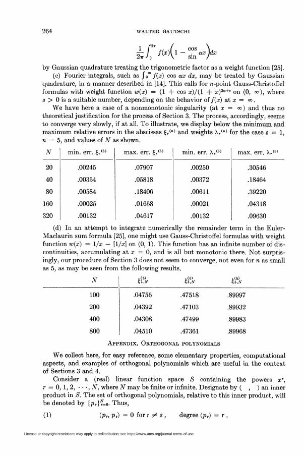
(c) Fourier integrals, such as J"o°° f(x) cos ax dx, may be treated by Gaussian

quadrature, in a manner described in [14]. This calls for n-point Gauss-Christoffel

formulas with weight function w(x) = (1 + cos x)/(l + x)2n+s on (0, go), where

s > 0 is a suitable number, depending on the behavior of f(x) at x = go .

We have here a case of a nonmonotonic singularity (at x = go) and thus no

theoretical justification for the process of Section 3. The process, accordingly, seems

to converge very slowly, if at all. To illustrate, we display below the minimum and

maximum relative errors in the abscissas £r(n) and weights Xr(n) for the case s = 1,

n = 5, and values of N as shown.

N

20

40

80

160

320

min. err. £r (5)

.00245

.00354

.00584

.00025

.00132

max. err. £r (.->)

.07907

.05818

.18406

.01658

.04617

min. err. Xr(5)

.00250

.00372

.00611

.00021

.00132

max. err. Xr(5)

.30546

.18464

.39220

.04318

.09630

(d) In an attempt to integrate numerically the remainder term in the Euler-

Maclaurin sum formula [25], one might use Gauss-Christoffel formulas with weight

function w(x) = 1/x — [1/x] on (0, 1). This function has an infinite number of dis-

continuities, accumulating at x = 0, and is all but monotonie there. Not surpris-

ingly, our procedure of Section 3 does not seem to converge, not even for n as small

as 5, as may be seen from the following results.

N >(6)Ç1.AT

t(5)Ç3.N

t(5)Ç5.2V

100

200

400

800

.04756

.04392

.04308

.04510

.47518

.47103

.47499

.47361

.89997

.89932

.89983

.89968

Appendix. Orthogonal polynomials

We collect here, for easy reference, some elementary properties, computational

aspects, and examples of orthogonal polynomials which are useful in the context

of Sections 3 and 4.

Consider a (real) linear function space S containing the powers xT,

r = 0, 1, 2, • • •, N, where N may be finite or infinite. Designate by ( , ) an inner

product in S. The set of orthogonal polynomials, relative to this inner product, will

be denoted by {pr}f_o. Thus,

(1) (pr, p») = 0 for r ?¿ s , degree (pr) = r .


GAUSS-CHRISTOFFEL quadrature formulas 265

These polynomials are uniquely determined if we require that each pr has leading

coefficient one. The orthonormal polynomials will be denoted by p*. We have

(2) P*(X) = CrPr(x) , Cr = (pr, Pr)~112 .

1. Recurrence relations.

Theorem 1. The orthogonal polynomials in (1), having leading coefficients one,

satisfy the recurrence relation

(3) Pr+i(x) = (x — ar,r)Pr(x) — ar,r-iPr-\(x) — ■ ■ ■ — ar,oPo(x)

(r = 0, 1,2, ...,2V-1),

where

(4) ar,s = (xpr, Ps)/(ps, Ps) (s = 0,1,2, •• -,r).

Proof. It is clear that the polynomials defined by (3), and p<¡(x) = 1, have

leading coefficients one and correct degrees. A simple computation shows that

orthogonality of p0, pi, ■ ■ •, pr implies orthogonality of p0, pi, • • -, pr+i. Since

p0 and p\ are orthogonal, Theorem 1 follows by induction.

A recurrence relation for the orthonormal polynomials p* could be obtained in

the obvious manner by substituting (2) into (3). Computationally, it is slightly

more convenient to introduce

(5) Pr(x) = Cr-lPr(x) = Cr-lP*(x)/cr ,

and to transform (3), (4) into

(o*\ Pt+i(x) = (x — a*T,r)pr*(x) — a*r,r-\P%-\(x) — • • • — a^,0po*(x) ,

P*+l(x) = pr+l(x)/(pr+l, pr+lY ^ ,

where

a* s = (xpr*, p*) (s = 0, 1, • • •, r) .

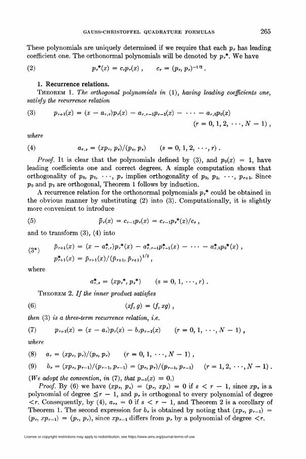
Theorem 2. // the inner product satisfies

(6) (xf, g) = (/, xg) ,

then (3) is a three-term recurrence relation, i.e.

(7) Pr+i(x) = (x — ar)pr(x) — brpr-i(x) (r = 0, 1, • • •, N — 1) ,

where

(8) ar = (xpr, Pr)/(Pr, Pr) (r = 0, 1, • • •, N - 1) ,

(9) bT = (Xpr, pr~l)/(Pr-l, Pr-l) = (pr, pr)/(Pr-l, Pr-l) (r = 1, 2, ■ ■ ■, N - 1) .

(We adopt the convention, in (7), that p~i(x) = 0.)

Proof. By (6) we have (xpr, ps) = (pr, xps) = 0 if s < r — 1, since xps is a

polynomial of degree £r — 1, and p, is orthogonal to every polynomial of degree

<r. Consequently, by (4), ars = 0 if s < r — 1, and Theorem 2 is a corollary of

Theorem 1. The second expression for br is obtained by noting that (xpr, Pr-i) =

(pr, xpr-i) = (pr, Pr), since xpr-i differs from pr by a polynomial of degree <r.


266 WALTER GAUTSCHI

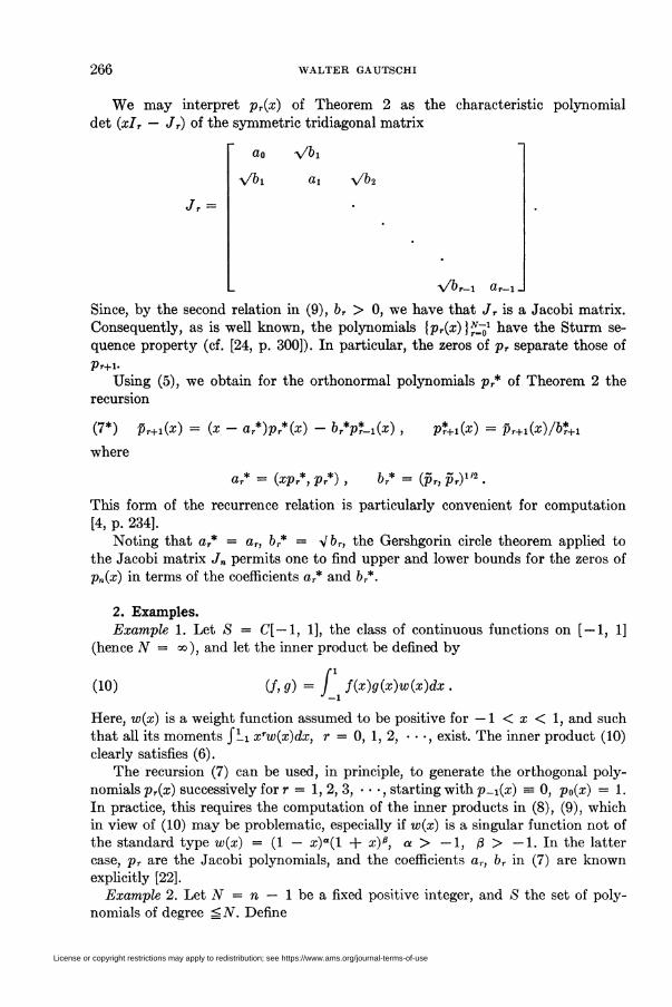
We may interpret pr(x) of Theorem 2 as the characteristic polynomial

det (xlr — Jr) of the symmetric tridiagonal matrix

Jr =

Qq

Vbi

Vbi

ax Vb2

y/br-i ar-i J

Since, by the second relation in (9), br > 0, we have that Jr is a Jacobi matrix.

Consequently, as is well known, the polynomials {pr(x)}^ have the Sturm se-

quence property (cf. [24, p. 300]). In particular, the zeros of pr separate those of

Pr+l.

Using (5), we obtain for the orthonormal polynomials pT* of Theorem 2 the

recursion

(7*) Pr+iG*0 = (x - ar*)pr*(x) - br*p*-i(x) , p*+i(x) = pr+i(x)/b*+1

where

Or* = (xpr*, P*) , br* = (Pr, Pr)1'2 .

This form of the recurrence relation is particularly convenient for computation

[4, p. 234].Noting that ar ar, br* ■Jbr, the Gershgorin circle theorem applied to

the Jacobi matrix Jn permits one to find upper and lower bounds for the zeros of

pn(x) in terms of the coefficients ar* and br*.

2. Examples.

Example 1. Let S = C[— 1, 1], the class of continuous functions on [—1, 1]

(hence N = go), and let the inner product be defined by

(10) (/:; g) = f f(x)g(x)w(x)dx,

Here, w(x) is a weight function assumed to be positive for —1 < x < 1, and such

that all its moments Jli xrw(x)dx, r = 0, 1, 2, • • -, exist. The inner product (10)

clearly satisfies (6).

The recursion (7) can be used, in principle, to generate the orthogonal poly-

nomials pr(x) successively for r = 1, 2, 3, • • -, starting with p-i(x) = 0, pa(x) = 1.

In practice, this requires the computation of the inner products in (8), (9), which

in view of (10) may be problematic, especially if w(x) is a singular function not of

the standard type w(x) = (1 — x)"(l + x)ß, a > —1, ß > —1. In the latter

case, pr are the Jacobi polynomials, and the coefficients ar, br in (7) are known

explicitly [22].

Example 2. Let N = n — 1 be a fixed positive integer, and S the set of poly-

nomials of degree ^ N. Define



(H) (f,g)=T,Wrf(Xr)g(Xr),r-1

where wr, xr are fixed real numbers with wT > 0, xr 9e xs for r ¿¿ s. We note that

S is an inner product space, since (f, f) =0 implies f(xT) = 0 (r = 1, 2, • • •, n),

which in turn implies/ = 0, / being a polynomial of degree <n.

In contrast to Example 1, we now have a finite set of orthogonal polynomials

depending on a parameter, n. To different values of n correspond different sets of

orthogonal polynomials. As (6) is satisfied, these polynomials again obey the re-

lations in (7)-(9). The successive computation of the coefficients ar, br is now

straightforward, since the inner product (11) requires only the evaluation of a

finite sum.

Example 3. Let N = 2n — 1 be fixed, and S the set of polynomials of degree

g N. Definen

(12) (/, g) = E [urf(xr)g(xT) + vrf (xT)g'(xr)] ,r=l

where uT, vr, xr are fixed real numbers, with ur > 0, vr > 0. As in Example 2 one

shows that S is an inner-product space. Unlike the previous example, however,

the inner product now fails to satisfy (6). As a result, the associated orthogonal

polynomials pT obey the "long" recurrence relation (3). The coefficients ar,s ap-

pearing in this relation are different from zero, in general, although in special

circumstances some of them may vanish (cf. Theorem 3 below).

While it is true that the recurrence relation is now more complicated, it can

still be used, as in Example 2, to successively build up the coefficients ar,,. The

inner products required in (4) are readily computed by the finite summation in

(12), using for the derivatives the recursion

(13) p'r+i(x) = Pr(x) + Or — ar.r)Pr'(x) — ar,r-ip'r-i(x) — ••• — ar,ipi'(x) .

We remark that the continuous analogues of the polynomials considered in

Example 3 were recently studied by Gröbner [12].

3. Symmetry Properties. If w(x) is an even function on (—a, a), where 0 < a

^ go , then the associated orthogonal polynomials satisfy

PAX) = (-l)rPr(-x) .

In particular, the zeros of pr are located symmetrically with respect to the origin,

and x = 0 is a zero of pT if r is odd.

This property may be used to essentially cut in half the amount of work re-

quired to construct the Christoffel numbers for an even weight function. Indeed,

the polynomials pn,e(x) — p2n(^x) form a set of orthogonal polynomials relative

to the inner product

(f,g)e = f f(x)g(x)^^-dx'o Vx

It follows that the Christoffel numbers £T% \Tn?, of p„,e are related to those of p2n by

«ft = [|?T, XÄi = 2Xr(2n> (r = 1,2, • • •, n) ,

where £r(2"> are the positive zeros of p2n and \<2n) the corresponding weight factors.


268 WALTER GAUTSCHI

Similarly, the polynomials pn,o(x) = (1/ V x)p2n+\( V x) are orthogonal with re-

spect to the inner product

(f,g)o= f(x)g(x)Vxw(Vx)dx,J 0

and their zeros and weight factors are given by

Un) i> (2n+l)-i2 , (n) otM\ <2"+D /„ 1 O ™ \Cr,0 = [Kr J , Xr,0 = 2?r,0Ar (f = 1,2, • • -, W) .

Here again £r(2n+1) denotes the positive zeros of p2K+i and Xr(2"+1) the corresponding

weight factors. Moreover,

/" u>(a;)dz - ¿ Xô/ô = X0<2"+1)•'-a r=l

is the weight factor corresponding to the zero £o(2n+1) = 0 of p2n+i.

The inner product (12) may be called equilibrated if

X/i+1—r X\ ~T" *£» »Cr

(14) (r = l,2, ...,n).

Wn+l-r == Ur, Vn+i—r — Vr

Theorem 3. // the inner product (12) is equilibrated, in the sense of (14), then the

associated orthogonal polynomials pr satisfy

(15) Pr(Xx + Xn — X) = (-l)rPr(x) .

Moreover, every other coefficient in the recursion (3) is zero, i.e.

(16) ar,r-2* = 0 (s = 1, 2, 3, •••).

The proof of Theorem 3 is elementary, and is omitted here.

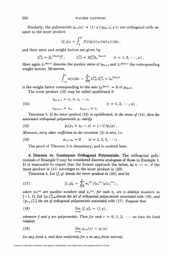
4. Discrete vs. Continuous Orthogonal Polynomials. The orthogonal poly-

nomials of Example 2 may be considered discrete analogues of those in Example 1.

It is reasonable to expect that the former approach the latter, as n —> oo, if the

inner product in (11) converges to the inner product in (10).

Theorem 4. Let (/, g) denote the inner product in (10), and let

(17) [f,g]n= J2wrMf(XrM)g(XrM),r=l

where wrM are positive numbers and xrM, for each n, are n distinct numbers in

[ — 1, 1]. Let {pr}r=o denote the set of orthogonal polynomials associated with (10), and

\pr.n]"=o the set of orthogonal polynomials associated with (17). Suppose that

(18) lim [/, g]n = (f, g) ,n—»oo

whenever f and g are polynomials. Then for each r = 0, 1, 2, • • • we have the limit

relation

(19) lim Pr,n(x) = VAX)n—»oo

for any fixed x, and thus uniformly for x in any finite interval.



Proof. We begin with the observation that

n

\U,g]n\ ú Y,™™ max \f(x)\ ■ max \g(x)\r=l — lSxgl —ISiSI

for any continuous functions /, g, and therefore

(20) \\f,g]n\ ̂||/|| IMI [1,1]«.

The polynomials pr, by Theorem 2, satisfy (7)-(9), while the polynomials p,,»,

by the same theorem, satisfy

(21) pr+i,n(x) = (x — ar,„)pr,„(x) — &r,npr-i,n(a:) ,

with

/OON „ _ [XPr.n, Pr,n\n r _ lxPr,n, Pr—\,n\n\ ) ar,n — r i , Or,n r i •

[Pr,n, Pr.njn [Pr—l,n, Pr—l,n\n

Suppose now that (19) is true for r = s and r = s — 1. We want to show that

(19) holds for r = s + 1. For this it suffices to show that

(23) as,n—>a,, &«,„—>&„ (n—>co),

since by (21), this implies ps+i,n(x) —» (x — as)ps(x) — bsps-i(x) = pg+i(x).

We have

[Ps.n, Ps,n]n = [ps + (pS,n ~ Ps), Ps + (Ps.n ~ Ps)]n

(24)= [Ps, Ps]n + 2[ps, ps,n - Ps]n + [Ps.n ~ Ps, Ps.n ~ Ps]n ■

The first term on the right, by (18), has the limit (ps, pe) as n —> oo. To the second

term we apply (20), with the result that

|[P«, Ps.n - Ps]n\ á ||PS|| \\Ps.n ~ Ps\\[l, 1]» .

Since [1, l]n —> (1, 1), and ps.n —* ps (by assumption), we see that the bound on

the right tends to zero as n —> go . By the same reasoning, one shows that the last

term in (24) also tends to zero. Consequently,

lim [p5,n, ps,n]n = (ps, Ps) ■n—*to

In the same manner, analogous limit relations can be established for all the

other inner products appearing in (22), thus proving (23).

Since, trivially, po,„ —» po, P-i,n —■* p-i, the assertion (19) now follows by in-

duction.

Theorem 4 may also be obtained from a general theorem of B. Ft. Kripke [13]

on best approximation with respect to nearby norms, if one observes that xT —

pr,n(x) and xr — pT(x) are the best approximations to xr, from polynomials of

degree r — 1, in the norms of (17) and (10), respectively. The author is indebted

to Professor J. R. Rice for this remark.

Corollary. Let the zeros of pr(x), in increasing order, be denoted by

•ri(r>, x2M, • • -, Xrir), and the zeros ofpT,n(x), in the same order, by x^n, x^n, • • -, xrT)n.

Under the assumptions of Theorem 4, we have

(25) lim xst = x,M , lim pt,n(x%) = pt(xsM) (s = 1, 2, • • •, r; t < r) .n—*oo n—»oo


270 WALTER GAUTSCHI

Proof. The first relation in (25) follows from the continuity of the zeros of an

algebraic equation. The second relation follows from

PtAxi'l) - Pt(XsM) = [pt.n(Xst) - P<Wl)] + ÍPtUt) - Pt(x,M)]

by observing that \ptin(x(¡i) - p«(a#i)| á max_is*si \pt,n(x) - pt(x)\ -» 0

(n —> oo ) , and pt(xlt%) —» Pt(x,M) («—»»).

Computer Sciences Department

Purdue University

Lafayette, Indiana 47907

1. D. G. Anderson, "Gaussian quadrature formulae for Jo1 — \i\{x)f{x)dx," Math. Comp.v. 19, 1965, pp. 477-481. MR 31 #2826.

2. S. Chandrasekhar, Radiative Transfer, Oxford Univ. Press, 1950, Chapter II. MR 13,136.

3. E. B. Christoffel, "Sur une classe particulière de fonctions entières et de fractionscontinues," Ann. Mat. Pura Appl., (2), v. 8, 1877, pp. 1-10.

4. P. J. Davis, Interpolation and Approximation, Blaisdell, New York, 1963. MR 28 #393.5. P. J. Davis & P. Rabinowitz, "Ignoring the singularity in approximate integration,"

SI AM J. Numer. Anal, v. 2, 1965, pp. 367-383. MR 33 #3459.6. L. Fejér, "Mechanische Quadraturen mit positiven Cotesschen Zahlen," Math. Z., v.

37, 1933, pp. 287-309.7. C. F. Gauss, "Methodus nova integralium valores per approximationem inveniendi,"

Comment. Soc. Regiae Sei. Gottingensis Recentiores, v. 3, 1816; Werke, Vol. 3, pp. 163-196.8. W. Gautschi, "On inverses of Vandermonde and confluent Vandermonde matrices. II,"

Numer. Math., v. 5, 1963, pp. 425-430. MR 29 #1734.9. W. Gautschi, "Numerical quadrature in the presence of a singularity," SI AM J. Numer.

Anal, v. 4, 1967, pp. 357-362.10. W. Gautschi, "Algorithm, Gaussian quadrature formulas," Comm. ACM. (To appear.)11. G. H. Golub & J. H. Welsch, Calculation of Gauss Quadrature Rules, Comput. Sei. Dept.

Tech. Rep. No. CS 81, Stanford University, Calif., 1967.12. W. Gröbner, "Orthogonale Polynomsysteme die gleichzeitig mit f{x) auch deren Ab-

leitung/'(x) approximieren," Funktionalanalysis, Approximationstheorie, Numerische Mathematik,edited by L. Collatz, G. Meinardus, and H. Unger, Birkhäuser, Basel, 1967, pp. 24-32.

13. B. R. Kripke, "Best approximation with respect to nearby norms," Numer. Math., v.6, 1964, pp. 103-105. MR 29 #1483.

14. L. G. Kruglikova & V. I. Krylov, "Numerical Fourier transform," Dokl. Akad. NaukBSSR, v. 5, 1961, pp. 279-283v(Russian) MR 26 #886.

15. V. I. Krylov & L. T. Sul'gina, Handbook on Numerical Integration, "Nauka," Moscow,1966. (Russian)

16. P. Rabinowitz, "Gaussian integration in the presence of a singularity," SI AM J. Numer.Anal, v. 4, 1967, pp. 191-201.

17. J. R. Rice, "A theory of condition," SIAM J. Numer. Anal, v. 3, 1966, pp. 287-310.18. J. R. Rice & S. Rosen, "NAPSS—a numerical analysis problem solving system," Proc.

ACM 21st Nati. Conf., Los Angeles, Calif. (August 1966), Thompson, Washington, D. C, 1966,pp. 51-56.

19. H. Rutishauser, "On a modification of the QD-algorithm with Graeffe-type conver-gence," Proc. IFIP Congress 62, pp. 93-96, North-Holland, Amsterdam, 1963.

20. T. J. Stieltjes, "Quelques recherches sur la théorie des quadratures dites mécaniques,"Ann. Sei. Ecole Norm. Sup., (3), v. 1, 1884, pp. 409-426; Oevres Complètes, Vol. I, pp. 377-394.

21. A. H. Stroud & Don Secrest, Gaussian Quadrature Formulas, Prentice-Hall, EnglewoodCliffs, N. J., 1966. MR 34 #2185.

22. G. Szegö, Orthogonal Polynomials, Amer. Math. Soc. Colloq. Publ., Vol. 23, Amer. Math.Soc, Providence, R. I., 1959. MR 21 #5029.

23. J. Todd, "The condition of the finite segments of the Hubert matrix," Nat. Bur. StandardsAppl. Math. Ser., No. 39, U. S. Government Printing Office, Washington, D. C, 1954, pp. 109-116.MR 16, 861.

24. J. H. Wilkinson, The Algebraic Eigenvalue Problem, Clarendon Press, Oxford, 1965.MR 32 #1894.

25. I. Zamfirescu, "An extension of Gauss' method for the calculation of improper integrals,"Acad. R. P. Romîne Stud. Cere. Mat., v. 14, 1963, pp. 615-631. (Romanian) MR 32 #1906.


Documents

Construction of Gauss-Christ of fei Quadrature Formulas · 2012-05-01 · Construction of Gauss-Christ of fei Quadrature Formulas By Walter Gautschi* 1. ... are associated with the