Embed Size (px)
Citation preview

3/2/2012
1
Technical Coaching Program – Design for Six Sigma
AGENDA – DAY 1, (February 21, 2012) 7:30 AM : Introduction by Pratik Shah & Michele Ziegler7:45 AM : Introduction by Graeme Knox and Kyoyul Oh 8:15 AM : Introduction by Al Power , President & COO –Gates Corporation
8:30 AM : Class Begins11:30 AM : Lunch Break12:30 PM : Class Resumes4:30 PM : End of DAY 1
Ref. Page N/A
Slide # 1
Slide 2
(The Taguchi Approach)
Dates: Feb. 21 – July 5, 2012Sponsor: Gates Corporation, Rochester Hills, MI and Columbia, MO.
Welcome!
Class Starts at: 7:30 AM Instructor:Ranjit Roy (120226.1)
Participants:
Professional from Gates Corporation
Robust Product and Process DesignsRobust Product and Process Designs

3/2/2012
2
Robust Product and Process DesignsRobust Product and Process Designs
Gates Corporation Gates Corporation –– DFSS Technical DFSS Technical Coaching ProgramCoaching Program
3/2/2012
3
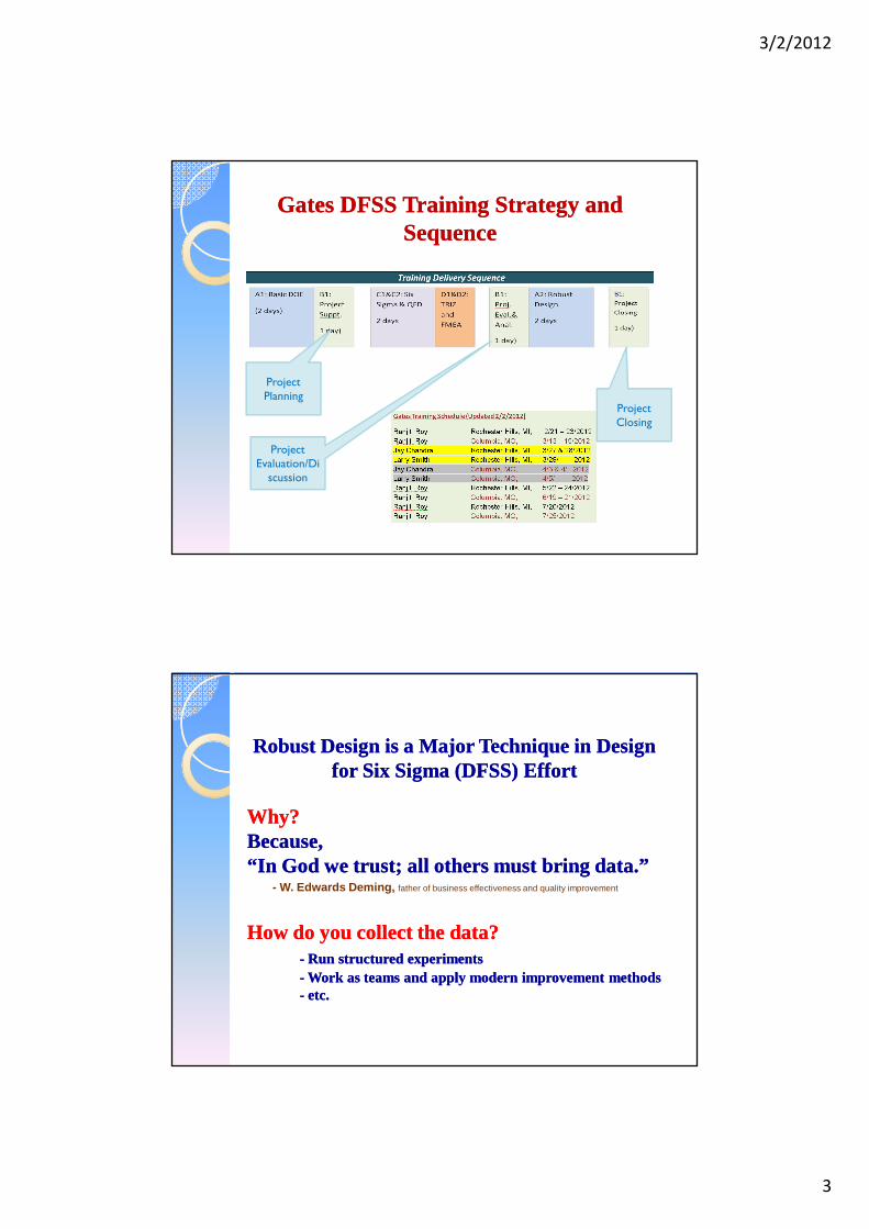
Gates DFSS Training Strategy and Gates DFSS Training Strategy and SequenceSequence
Project Planning
Project Closing
Project Evaluation/Di
scussion
Robust Design is a Major Technique in Design Robust Design is a Major Technique in Design for Six Sigma (DFSS) Effortfor Six Sigma (DFSS) Effort
Why?Why?Because, Because, “In God we trust; all others must bring“In God we trust; all others must bring data.”data.”
- W. Edwards Deming, father of business effectiveness and quality improvement
How do you collect the data?How do you collect the data?-- Run structuredRun structured experimentsexperiments-- WorkWork as teams and apply modern improvement methodsas teams and apply modern improvement methods-- etc.etc.

3/2/2012
4
◦ How To Design Experiments Using the Taguchi Approach.- Use Std. Orthogonal Array (Simple Designs) - Handle Interaction- Handle Mixed Levels- Includes Noise Factors (Robust Design)- Study Systems with Dynamic Response
◦ Steps in Analysis of Main Effects and determination of Optimum Condition.- Main effect studies- Interaction analysis- Analysis of Variance (ANOVA)- Signal to Noise ratio (S/N)- Dynamic Characteristics
◦ Learn to Quantify Improvements Expected From Improved Designs in Terms of Dollars. Apply Taguchi's loss function to compute $ LOSS.
◦ Learn to Brainstorm and Plan for Taguchi Experiments.- Determine evaluation criteria, factors, levels, interactions, noise factors, etc. by group consensus.
Course Content and Learning Objectives(Robust Design)
Slide # 7
Things you should learn from discussions in this mo dule:
◦ Why does performance vary?◦ What are NOISE FACTORS?◦ Why can’t we get rid of the Noise Factors?◦ How can we reduce variability without actually◦ removing the cause of variation?◦ What does an OUTER ARRAY design do?◦ Could you include the Noise Factors in your study◦ with the Control Factors?◦ What is an practical/economical strategy?
Strategies and Characteristics of Robust Design
Ref. Page 5 - 1
Slide # 8
3/2/2012
5
Instructor: Ranjit Roy
◦ Mechanical engineer
◦ Industrial experience since 1973.
◦ Independent consultant since 1987
◦ Specializes in product and process design improvement technique
◦ Published books and developed technical software
◦ Adjunct professor (Oakland University, Rochester, MI since 1976)
Introduction Ref. Page N/A
Slide # 9
Participants: Please tell us (address the class)
◦ Who you are, name
◦ Activities you are from or involved in
◦ Your reason for being in the class
◦ experience with quality improvement effort
◦ expectations you have
◦ Etc.
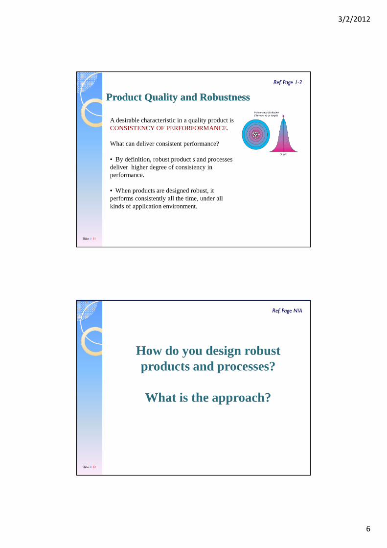
What is Robustness?What is Robustness?
Robust Product & Process designs
Sturdy, Rugged,Consistent, Dependable,..
What are examples of robust products and processes?
Why design robust products?Built Strong to Last Long
It takes the licking, but keeps on ticking
Ref. Page 1-1
Slide # 10
3/2/2012
6
Product Quality and RobustnessProduct Quality and Robustness
A desirable characteristic in a quality product is CONSISTENCY OF PERFORFORMANCE.
What can deliver consistent performance?
• By definition, robust product s and processes deliver higher degree of consistency in performance.
• When products are designed robust, it performs consistently all the time, under all kinds of application environment.
Ref. Page 1-2
Slide # 11
How do you design robust products and processes?
What is the approach?
Ref. Page N/A
Slide # 12
3/2/2012
7
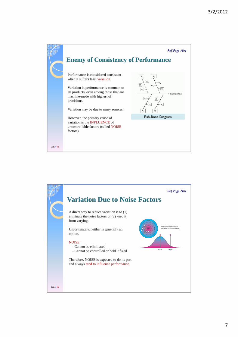
Enemy of Consistency of PerformanceEnemy of Consistency of Performance
Performance is considered consistent when it suffers least variation.
Variation in performance is common to all products, even among those that are machine-made with highest of precisions.
Variation may be due to many sources.
However, the primary cause of variation is the INFLUENCE of uncontrollable factors (called NOISEfactors)
Fish-Bone Diagram
Ref. Page N/A
Slide # 13
Variation Due to Noise FactorsVariation Due to Noise Factors
A direct way to reduce variation is to (1) eliminate the noise factors or (2) keep it from varying.
Unfortunately, neither is generally an option.
NOISE:- Cannot be eliminated- Cannot be controlled or held it fixed
Therefore, NOISE is expected to do its part and always tend to influence performance.
Ref. Page N/A
Slide # 14

3/2/2012
8
The Taguchi ApproachThe Taguchi Approach
“While NOISE often cannot be controlled or it is too expensive to control, perhaps, by some means, its INFLUENCE to performance can be minimized.”
How do you control its influence without controlling the noise factor itself?
Dr. Taguchi suggested a revolutionary idea.
- Leave noise alone- Find proper levels of the controllable factors to minimize influence of noise
Ref. Page N/A
Slide # 15
Robust Design StrategyRobust Design Strategy
Reduce variation by minimizing the influence of uncontrollable factors.
Determine design parameters by selecting a combination of the CONTROL FACTORS such that the performance is insensitive (immune) to the influence of UNCONTROLLABLE FACTORS.
“ Reduce variability without actually removing the cause of variability.”
Ref. Page N/A
Slide # 16

3/2/2012
9
Desired Output Characteristic Desired Output Characteristic
ROBUST DESIGN
Sensitive
O
U
T
P
U
T
Input/Signal
Less Sensitive
Ref. Page 1-3
Slide # 17
Robust Design Application MethodologiesRobust Design Application Methodologies
Methods: Undertake experimental studies with hardwareoranalytical simulation
When: The earlier the better. The return on investment is highest when applied in product design and development phases.
Specific Method:- Taguchi experimental design (PARAMETER DESIGN)- Outer array designs with NOISE factors (Process diagram & Ideal
function)- Analysis ( Two step optimization, Signal-to-noise, Loss function,
etc.)
(First part of this seminar will be dedicated to learning the experimental design techniques)
Ref. Page 1-3
Slide # 18

3/2/2012
10
History of Quality Improvement History of Quality Improvement Activities and the Taguchi Activities and the Taguchi
Experimental Design TechniquesExperimental Design Techniques
Ref. Page N/A
Slide # 19
Quality & Cost Improvement Quality & Cost Improvement -- Lean Manufacturing History (Timeline )Lean Manufacturing History (Timeline )
1850 1875 1900 1920 1940 1960 1980 2000
WW-I WW-IICivil War
Eli Whitney1765 – 1825, was an American inventor and manufacturer who is credited with creating the first cotton gin in 1793. • Interchangeable parts
Henry Ford•Assembly Line•Flow Lines•Manufacturing Strategy
Eiji Toyoda Taichi Ohno Shigeo Shingo
•Just in Time and Toyota Production System
•Stockless Production
•World Class Manufacturing
Fredrick Taylor• Standardized work time study & work standards• Worker/management dichotomy
Frank & Lilian Gilbreth•Process Chart•Motion Study
Edward Joseph Genichi Kaoru Deming Juran Taguchi Ishikawa
•TQM, SPC, Taguchi Methods, Fishbone Diagram ….
Ref. Page N/A
Slide # 20

3/2/2012
11
Module – 1Overview of the Taguchi
Experimental Design Approach
Slide # 21
� Genichi Taguchi was born in Japan in 1924.
� Worked with Electronic Communication Laboratory (ECL) of Nippon Telephone and Telegraph Co.(1949 -61).
� Major contribution has been to standardize and simplify the use of the DESIGN OF EXPERIMENTS techniques.
� Published many books and papers on the subject.
Who is Taguchi?Ref. Page 1- 4
22Slide # 22
3/2/2012
12
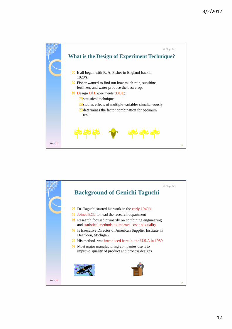
� It all began with R. A. Fisher in England back in 1920’s.
� Fisher wanted to find out how much rain, sunshine, fertilizer, and water produce the best crop.
� Design Of Experiments (DOE):
statistical technique
studies effects of multiple variables simultaneously
determines the factor combination for optimum result
What is the Design of Experiment Technique?
Ref. Page 1- 4
23Slide # 23
� Dr. Taguchi started his work in the early 1940’s
� Joined ECL to head the research department
� Research focused primarily on combining engineering and statistical methods to improve cost and quality
� Is Executive Director of American Supplier Institute in Dearborn, Michigan
� His method was introduced here in the U.S.A in 1980
� Most major manufacturing companies use it to improve quality of product and process designs
Background of Genichi TaguchiRef. Page 1- 5
24Slide # 24
3/2/2012
13
� DO IT UP-FRONT:
Return on investment higher in design
The best way is to build quality into the design
� DO IT IN DESIGN. DESIGN QUALITY IN:
Does not replace quality activities in production
Must not forget to do quality in design
What’s New? Philosophy !Ref. Page 1- 5
25Slide # 25
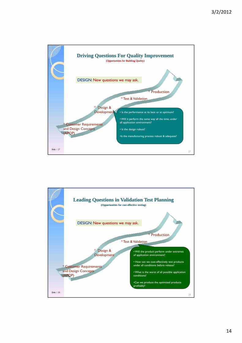
Product Engineering Roadmap (Opportunities for Building Quality)
Where do we do quality improvement?
* Design & Analysis
* Design & Development
* Test & Validation
* Production
Return on Investment
Ref. Page 1- 6
Slide # 26
3/2/2012
14
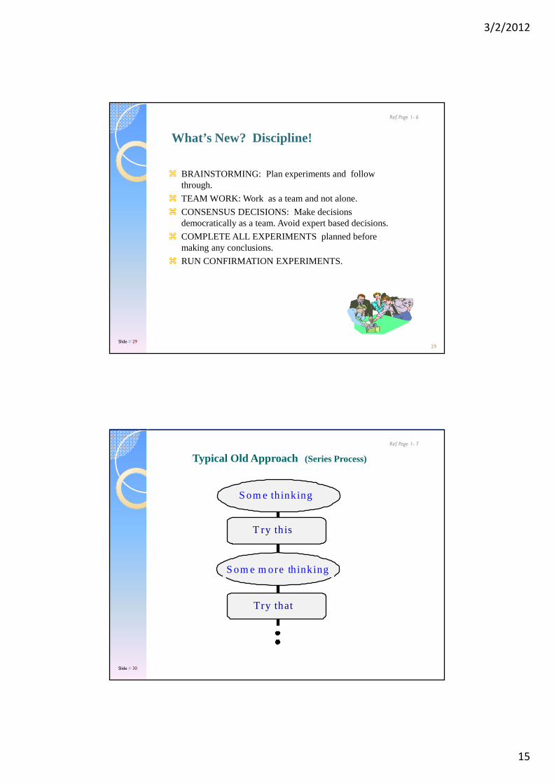
Driving Questions For Quality ImprovementDriving Questions For Quality Improvement(Opportunities for Building Quality)(Opportunities for Building Quality)
* Customer Requirements and Design Concepts (APQP)
* Design & Development
* Test & Validation
* Production
• Is the performance at its best or at optimum?
• Will it perform the same way all the time, under all application environment?
• Is the design robust?
•Is the manufacturing process robust & adequate?
DESIGN: New questions we may ask.
27Slide # 27
Leading Questions in Validation Test PlanningLeading Questions in Validation Test Planning(Opportunities for cost(Opportunities for cost--effective testing)effective testing)
* Customer Requirements and Design Concepts (APQP)
* Design & Development
* Test & Validation
* Production
• Will the product perform under extremes of application environment?
• How can we cost-effectively test products under all conditions before release?
• What is the worst of all possible application conditions?
•Can we produce the optimized products profitably?
28Slide # 28
DESIGN: New questions we may ask.
3/2/2012
15
� BRAINSTORMING: Plan experiments and follow through.
� TEAM WORK: Work as a team and not alone.
� CONSENSUS DECISIONS: Make decisions democratically as a team. Avoid expert based decisions.
� COMPLETE ALL EXPERIMENTS planned before making any conclusions.
� RUN CONFIRMATION EXPERIMENTS.
What’s New? Discipline!
Ref. Page 1- 6
29Slide # 29
Som e th inking
Som e m ore think ing
T ry th is
Try that
Typical Old Approach (Series Process)
Ref. Page 1- 7
Slide # 30
3/2/2012
16
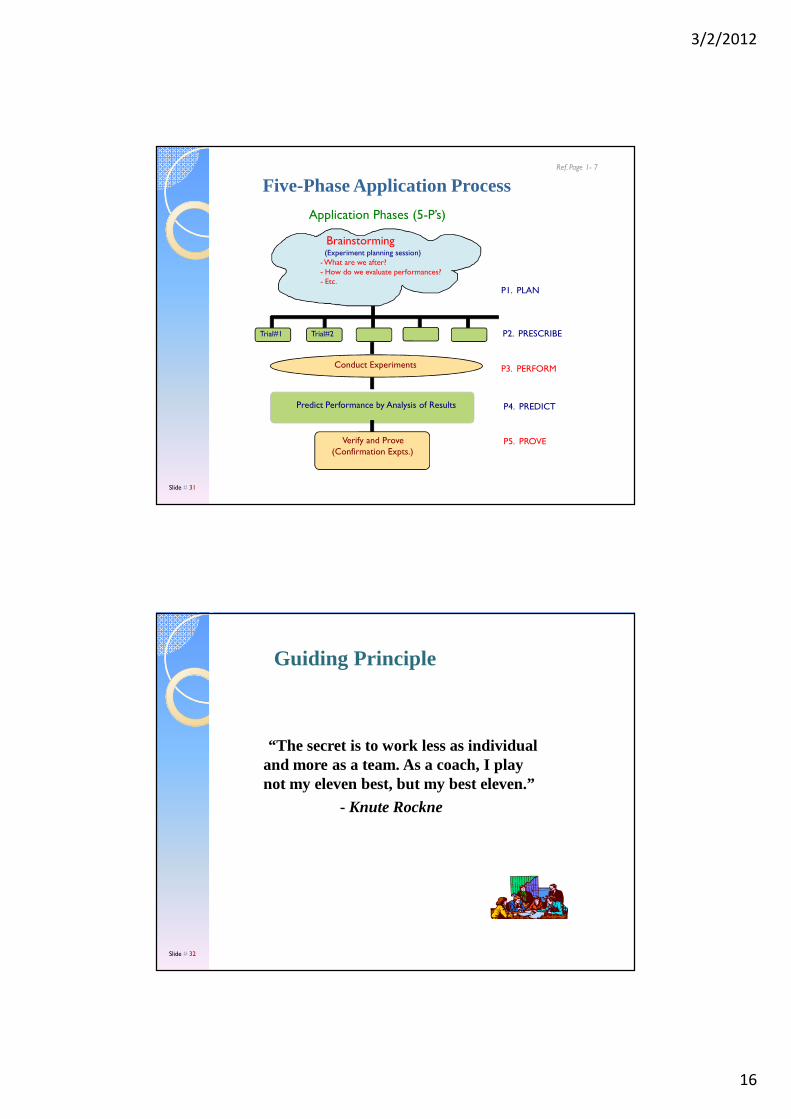
Brainstorming
Trial#1 Trial#2
Predict Performance by Analysis of Results
P1. PLAN
P2. PRESCRIBE
P3. PERFORM
P4. PREDICT
P5. PROVE
Application Phases (5-P’s)
Verify and Prove (Confirmation Expts.)
Conduct Experiments
(Experiment planning session)-What are we after?- How do we evaluate performances?- Etc.
Five-Phase Application ProcessRef. Page 1- 7
Slide # 31
“The secret is to work less as individual and more as a team. As a coach, I play not my eleven best, but my best eleven.”
- Knute Rockne
Guiding Principle
Slide # 32

3/2/2012
17
� CONSISTENCY OF PERFORMANCE: Quality may be viewed in terms of consistency of performance. To be consistent is to BE LIKE THE GOOD ONE’S ALL THE TIME.
� REDUCED VARIATION AROUND THE TARGET: Quality of performance can be measured in terms of variations around the target.
What’s New? Definition of QualityRef. Page 1- 8
This holds true also with performance of
any product or process.
33Slide # 33
Looks of ImprovementLooks of ImprovementFigure 1: Performance Before Experimental Study Figure 2: Performance After Study
m = (Yavg -Yo )
Yavg. Yo
σσnew
Improve Performance = Reduce σ and/or Reduce m
34Slide # 34
Ref. Page 1- 8
3/2/2012
18
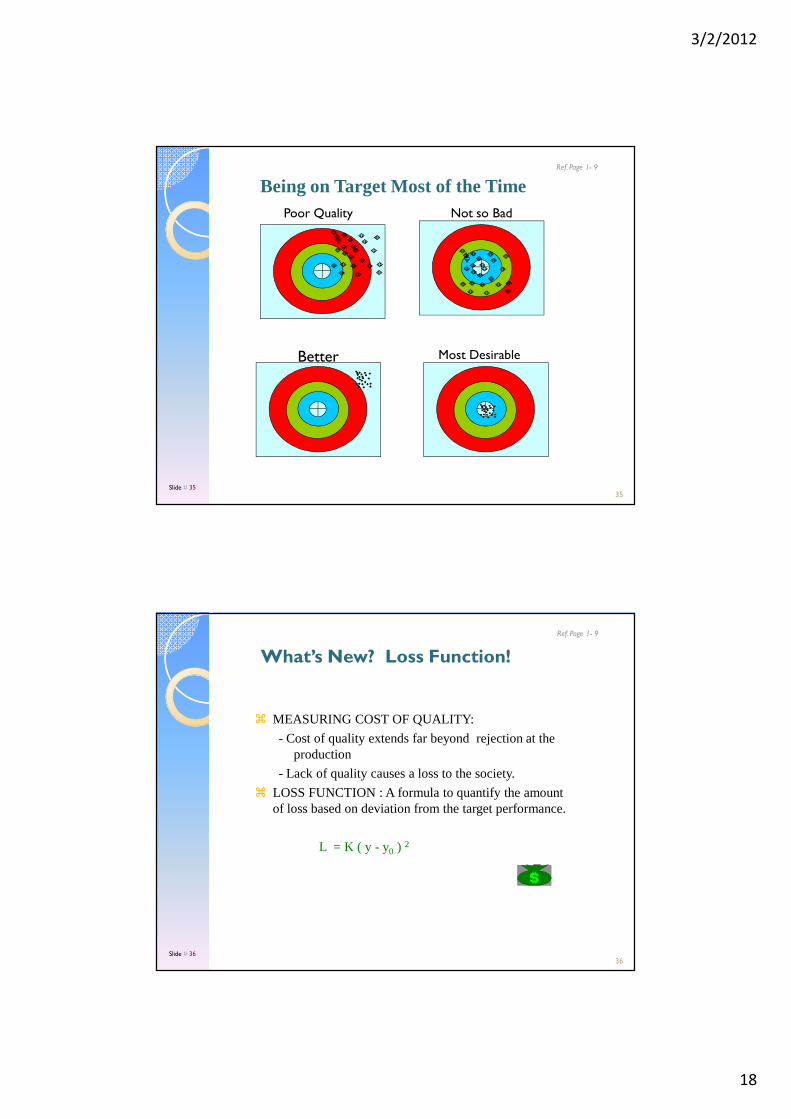
Poor Quality Not so Bad
Better Most Desirable
Being on Target Most of the Time Ref. Page 1- 9
35Slide # 35
� MEASURING COST OF QUALITY:
- Cost of quality extends far beyond rejection at the production
- Lack of quality causes a loss to the society.
� LOSS FUNCTION : A formula to quantify the amount of loss based on deviation from the target performance.
L = K ( y - y0 ) 2
What’s New? Loss Function!
Ref. Page 1- 9
36Slide # 36

3/2/2012
19
� APPLICATION STEPS: Steps for applications are clearly defined.
� EXPERIMENT DESIGNS: Experiments are designed using special orthogonal arrays.
� ANALYSIS OF RESULTS: Analysis and conclusions follow standard guidelines.
What’s New? Simpler and Standardized DOE.
Ref. Page 1- 10
37Slide # 37
“Things should be as simple as possible,
but no simpler.”- Albert Einstein
Simpler and Standardized DOE Methodologies
Ref. N/A
38Slide # 38

3/2/2012
20
� PARAMETER DESIGN: Taguchi approach generally refers to the parameter design phase of the three quality engineering activities (SYSTEM DESIGN, PARAMETER DESIGN and TOLERANCE DESIGN) proposed by Taguchi.
� Off-line Quality Control
� Quality Loss Function
� Signal To Noise Ratio(s/n) For Analysis
� Reduced Variability, a Measure Of Quality
DOE - the Taguchi Approach - Seminar ContentsRef. Page 1- 11
39Slide # 39
EXAMPLE APPLICATION
� It is an experimental technique that determines the solution with minimum effort.
� In a POUND CAKE baking process with 5 ingredients, and with options to take HIGH and LOW values of each, it can determine the recipe with only 8 experiments.
� Full factorial calls for 32 experiments. Taguchi approach requires only 8
How Does DOE Technique Work?
Ref. Page 1- 11
40Slide # 40
3/2/2012
21
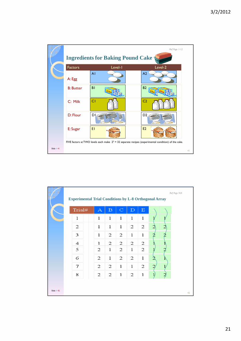
FIVE factors at TWO levels each make 25 = 32 separate recipes (experimental condition) of the cake.
Ingredients for Baking Pound Cake
Factors Level-1 Level-2
A: Egg
B: Butter
C: Milk
E: Sugar
D: Flour
A2A1
B1 B2
C1 C2
D2D1
E1 E2
Ref. Page 1-12
41Slide # 41
Experimental Trial Conditions by L-8 Orthogonal Arr ay
Ref. Page N/A
42Slide # 42
3/2/2012
22
Experiment Design Using L-8 ArrayRef. Page N/A
43Slide # 43
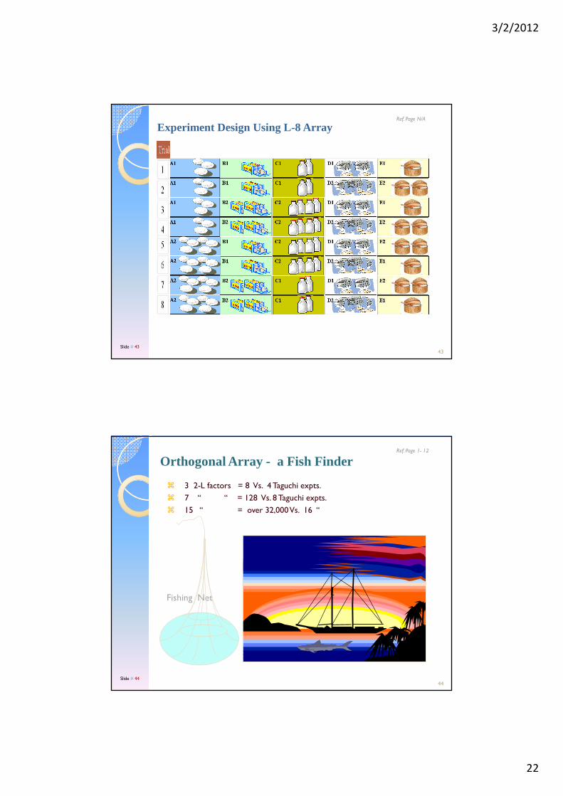
� 3 2-L factors = 8 Vs. 4 Taguchi expts.
� 7 ‘‘ ‘‘ = 128 Vs. 8 Taguchi expts.
� 15 ‘‘ = over 32,000 Vs. 16 ‘‘
Fishing Net
Orthogonal Array - a Fish FinderRef. Page 1- 12
44Slide # 44

3/2/2012
23
� Standardized application and data analysis
� Higher probability of success
� Option to confirm predicted improvement
� Improvement quantified in terms of dollars
Benefits of the Taguchi DOE?
Ref. Page 1- 12
45Slide # 45
Desirable Goals and Objectives for Manufacturing Quality Products
Ref. Page 1- 12
46Slide # 46
What matters is:: What you doMission: Find the Rights THINGS to do
Activity areas and objectives:
What matters is:How you do itMission: Do the Things RIGHT
Activity Areas and objectives:
A: Product Definition and Concept Designs
B: Design & Development
C: Performance Validation
D: Production
- Search for market demand
- Determine products to make
- Define design specifications
- Design parts- Optimize designs- Build robustness
- Build and test prototypes- Perform test to validate robustness
- Optimize process- Reduce variability and rejects
Problem Type ====> - Technical problems with performance- Understanding sources of influence and behaviors
- Establishing level of performance- Validating for robust performance
- Rejects & rework- Warranty & customer satisfaction- Process robustness
3/2/2012
24
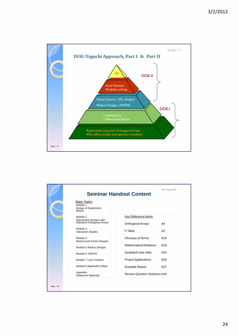
•Experiment using Std. Orthogonal Arrays•Main effect studies and optimum condition
• Interactions• Mixed level factors
•Loss Function •Problem solving
DC
•Noise Factors, S/N, Analysis
•Robust Designs, ANOVA
DOE-II
DOE-I
DOE/Taguchi Approach, Part I & Part II
Ref. Page 1- 15
Slide # 47
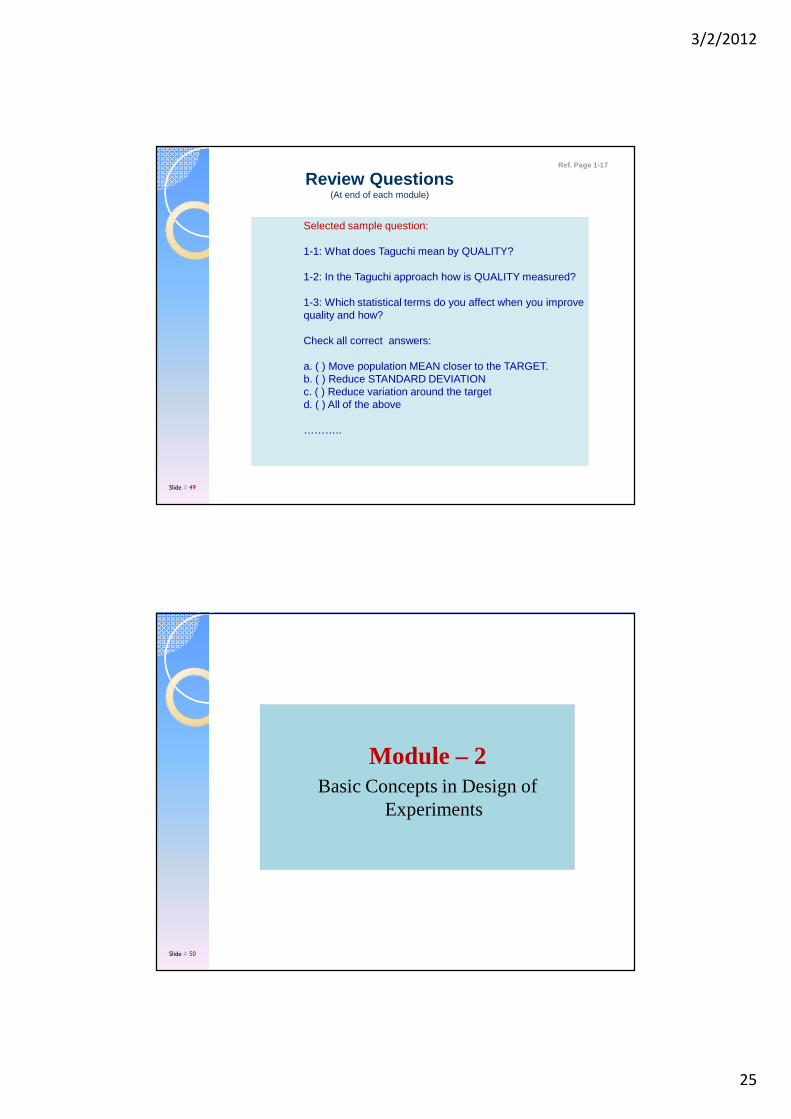
Seminar Handout Content
Key Reference Items
Orthogonal Arrays A4
F-Table A2
Glossary of Terms A16
Mathematical Relations A18
Qualitek4 User Help A22
Project Applications A25
Example Report A27
Review Question Solutions A34
Major TopicsModule 1Design of Experiment Basics
Module 2Experiment Designs with Standard Orthogonal Arrays
Module 3Interaction Studies
Module 4Mixed-Level Factor Designs
Module 5 Robust Designs
Module 6 ANOVA
Module 7 Loss Function
Module 8 Application Steps
AppendixReference Materials
Ref. Page N/A
Slide # 48
3/2/2012
25
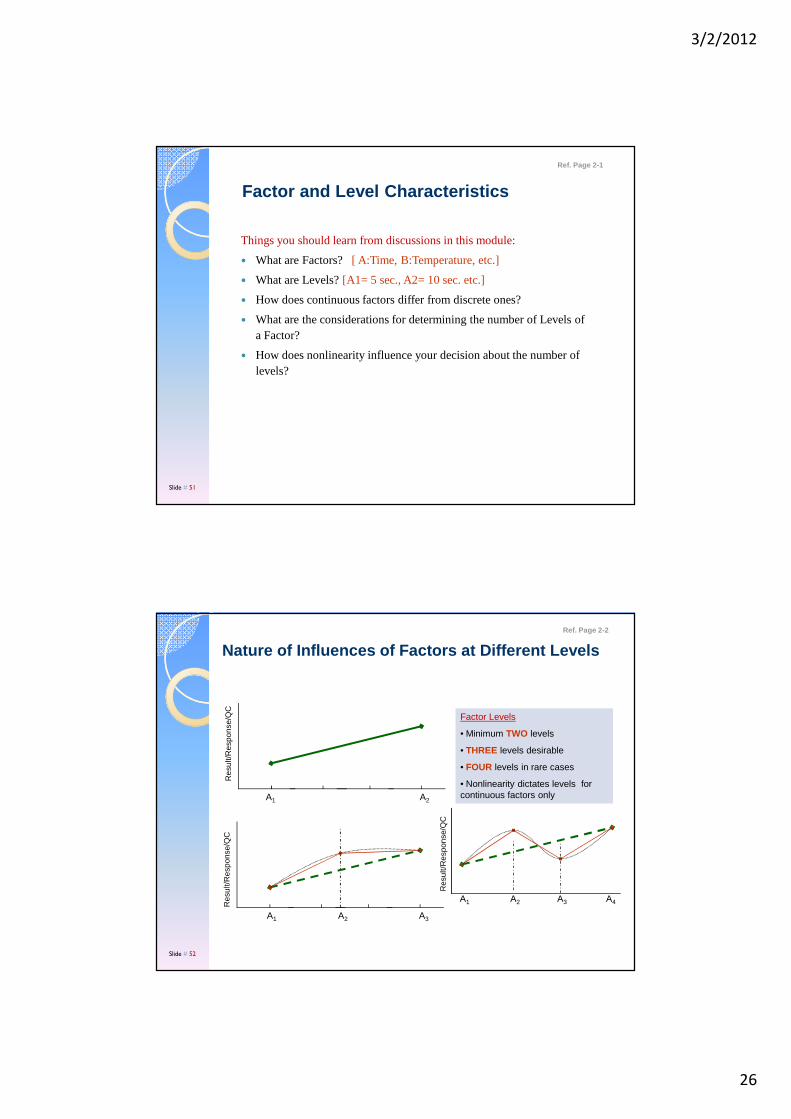
Selected sample question:
1-1: What does Taguchi mean by QUALITY?
1-2: In the Taguchi approach how is QUALITY measured?
1-3: Which statistical terms do you affect when you improve quality and how?
Check all correct answers:
a. ( ) Move population MEAN closer to the TARGET.b. ( ) Reduce STANDARD DEVIATIONc. ( ) Reduce variation around the targetd. ( ) All of the above
………..
Review Questions(At end of each module)
Ref. Page 1-17
Slide # 49
Module – 2Basic Concepts in Design of
Experiments
Slide # 50
3/2/2012
26
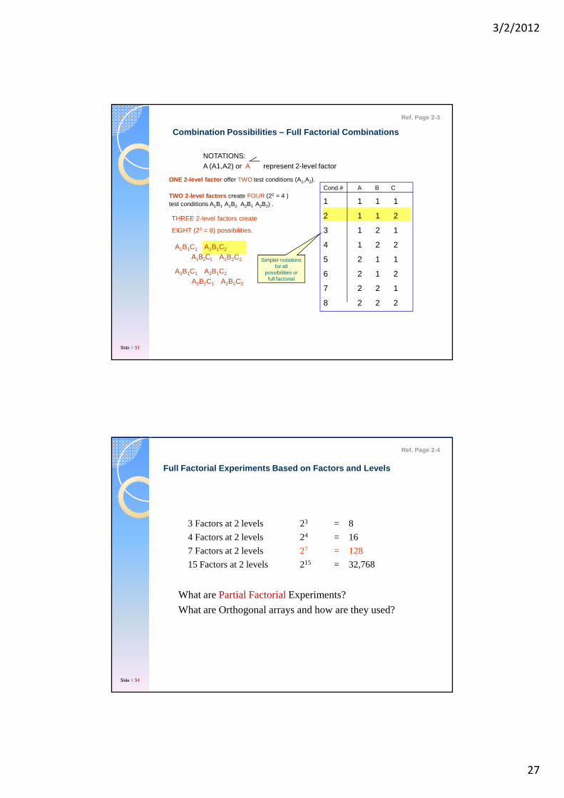
Things you should learn from discussions in this module:
� What are Factors? [ A:Time, B:Temperature, etc.]
� What are Levels? [A1= 5 sec., A2= 10 sec. etc.]
� How does continuous factors differ from discrete ones?
� What are the considerations for determining the number of Levels of a Factor?
� How does nonlinearity influence your decision about the number of levels?
Factor and Level Characteristics
Ref. Page 2-1
Slide # 51
Nature of Influences of Factors at Different Levels
Res
ult/R
espo
nse/
QC
A1 A2 A3 A2
Res
ult/R
espo
nse/
QC
A1 A2 A3
Factor Levels
• Minimum TWO levels
• THREE levels desirable
• FOUR levels in rare cases
• Nonlinearity dictates levels for continuous factors only
Res
ult/R
espo
nse/
QC
A1 A2 A3 A4
Ref. Page 2-2
Slide # 52
3/2/2012
27
Combination Possibilities – Full Factorial Combinati ons
ONE 2-level factor offer TWO test conditions (A1,A2).
TWO 2-level factors create FOUR (22 = 4 ) test conditions A1B1 A1B2 A2B1 A2B2) .
NOTATIONS:A (A1,A2) or A represent 2-level factor
THREE 2-level factors create
EIGHT (23 = 8) possibilities.
A1B1C1 A1B1C2
A1B2C1 A1B2C2
A2B1C1 A2B1C2
A2B2C1 A2B2C2
Simpler notations for all
possibilities or full factorial
Cond.# A B C
1 1 1 1
2 1 1 2
3 1 2 1
4 1 2 2
5 2 1 1
6 2 1 2
7 2 2 1
8 2 2 2
Ref. Page 2-3
Slide # 53
3 Factors at 2 levels 23 = 8
4 Factors at 2 levels 24 = 16
7 Factors at 2 levels 27 = 128
15 Factors at 2 levels 215 = 32,768
What are Partial Factorial Experiments?
What are Orthogonal arrays and how are they used?
Full Factorial Experiments Based on Factors and Lev els
Ref. Page 2-4
Slide # 54
3/2/2012
28
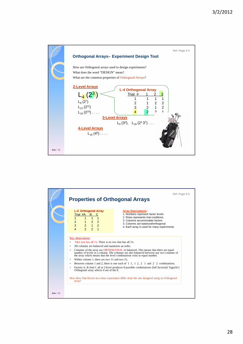
How are Orthogonal arrays used to design experiments?
What does the word “DESIGN” mean?
What are the common properties of Orthogonal Arrays?
Orthogonal Arrays– Experiment Design Tool
2-Level Arrays
L4 (23 )L8 (27)L12 (211)L16 (215) . . . .
3-Level ArraysL9 (34), L18 (21 37) . . .
4-Level ArraysL16 (45) . . . .
L-4 Orthogonal ArrayTrial # 1 2 3
1 1 1 12 1 2 23 2 1 2 4 2 2 1
Ref. Page 2-4
Slide # 55
Key observations:
� First row has all 1's. There is no row that has all 2's.
� All columns are balanced and maintains an order.
� Columns of the array are ORTHOGONALor balanced. This means that there are equal number of levels in a column. The columns are also balanced between any two columns of the array which means that the level combinations exist in equal number.
� Within column 1, there are two 1's and two 2's.
� Between column 1 and 2, there is one each of 1 1, 1 2, 2 1 and 2 2 combinations.
� Factors A, B And C all at 2-level produces 8 possible combinations (full factorial) Taguchi’s Orthogonal array selects 4 out of the 8.
How does One-Factor-at-a-time experiment differ from the one designed using an Orthogonal array?
L-4 Orthogonal ArrayTrial #A B C1 1 1 12 1 2 23 2 1 2 4 2 2 1
Array Descriptions :1. Numbers represent factor levels2. Rows represents trial conditions3. Columns accommodate factors 3. Columns are balanced/orthogonal 4. Each array is used for many experiments
Properties of Orthogonal ArraysRef. Page 2-5
Slide # 56
3/2/2012
29
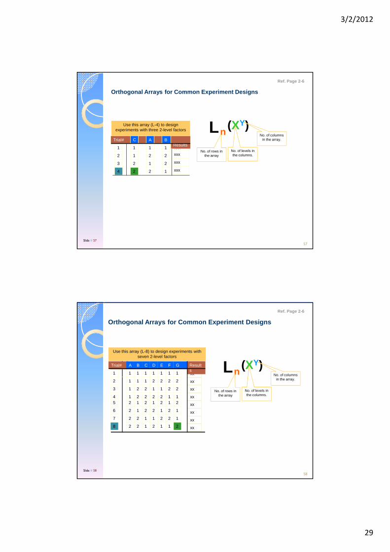
Orthogonal Arrays for Common Experiment Designs
L (XY)n
No. of rows in the array
No. of levels in the columns.
No. of columns in the array.
Use this array (L-4) to design experiments with three 2-level factors
1
1
2
2
1
2
2
1
1
2
1
2
1
2
4
3
xxx
xxx
xxx
xxx
C A BTrial#Results
Ref. Page 2-6
57Slide # 57
Orthogonal Arrays for Common Experiment Designs
L (XY)n
No. of rows in the array
No. of levels in the columns.
No. of columns in the array.
Use this array (L-8) to design experiments with seven 2-level factors
xx
xx
xx
xx
xx
xx
xx
xx
1
1
1
1
2
2
2
2
1
2
4
3
5
6
8
7
1
2
1
2
2
1
2
1
1
1
2
2
2
2
1
1
1
2
2
1
1
2
2
1
1
2
2
1
2
1
1
2
1
2
1
2
1
2
1
2
1
1
2
2
1
1
2
2
Results
ETrial# A CB FD G
Ref. Page 2-6
58Slide # 58
3/2/2012
30
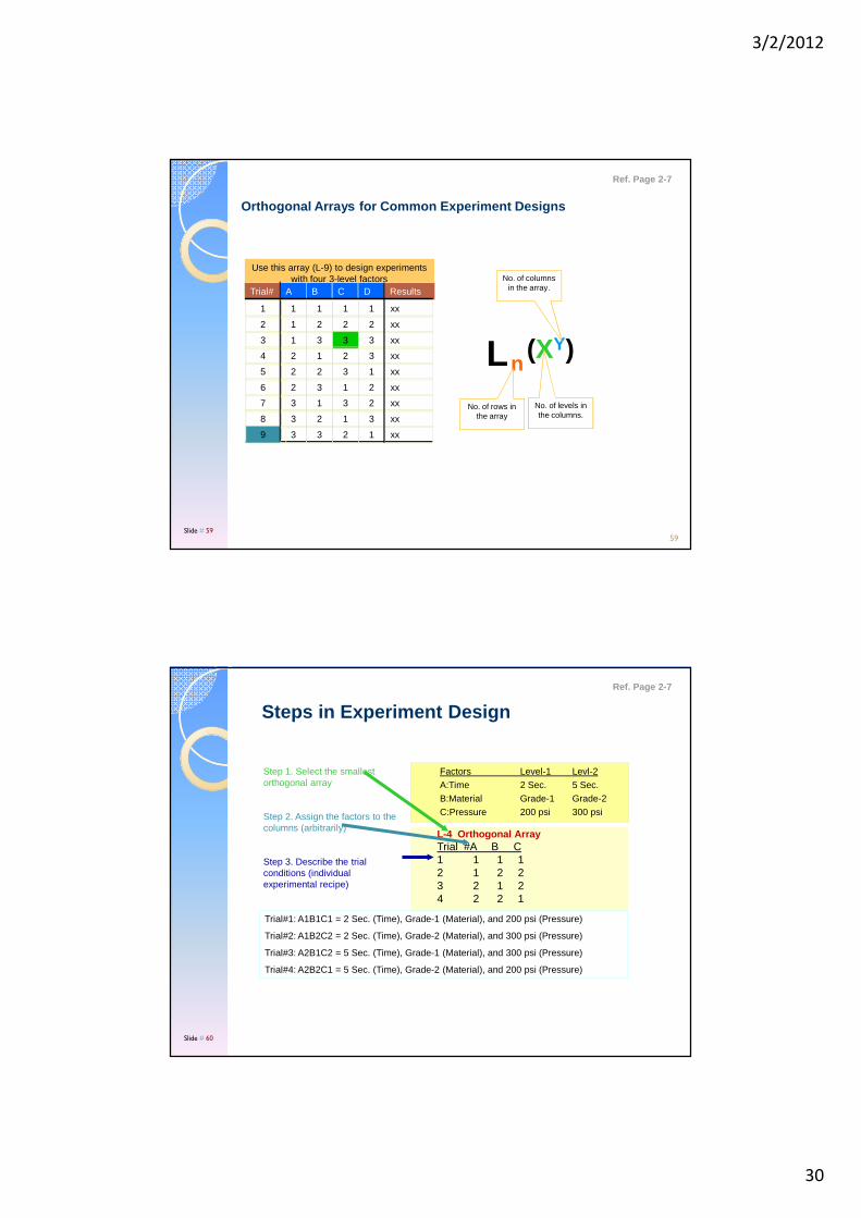
Orthogonal Arrays for Common Experiment Designs
L (XY)n
No. of rows in the array
No. of levels in the columns.
No. of columns in the array.
Use this array (L-9) to design experiments with four 3-level factors
Trial# A B C D Results
1 1 1 1 1 xx
2 1 2 2 2 xx
3 1 3 3 3 xx
4 2 1 2 3 xx
5 2 2 3 1 xx
6 2 3 1 2 xx
7 3 1 3 2 xx
8 3 2 1 3 xx
9 3 3 2 1 xx
Ref. Page 2-7
59Slide # 59
Steps in Experiment Design
Factors Level-1 Levl-2A:Time 2 Sec. 5 Sec.B:Material Grade-1 Grade-2C:Pressure 200 psi 300 psi
L-4 Orthogonal ArrayTrial #A B C1 1 1 12 1 2 23 2 1 2 4 2 2 1
Step 1. Select the smallest orthogonal array
Step 2. Assign the factors to the columns (arbitrarily)
Step 3. Describe the trial conditions (individual experimental recipe)
Trial#1: A1B1C1 = 2 Sec. (Time), Grade-1 (Material), and 200 psi (Pressure)
Trial#2: A1B2C2 = 2 Sec. (Time), Grade-2 (Material), and 300 psi (Pressure)
Trial#3: A2B1C2 = 5 Sec. (Time), Grade-1 (Material), and 300 psi (Pressure)
Trial#4: A2B2C1 = 5 Sec. (Time), Grade-2 (Material), and 200 psi (Pressure)
Ref. Page 2-7
Slide # 60
3/2/2012
31
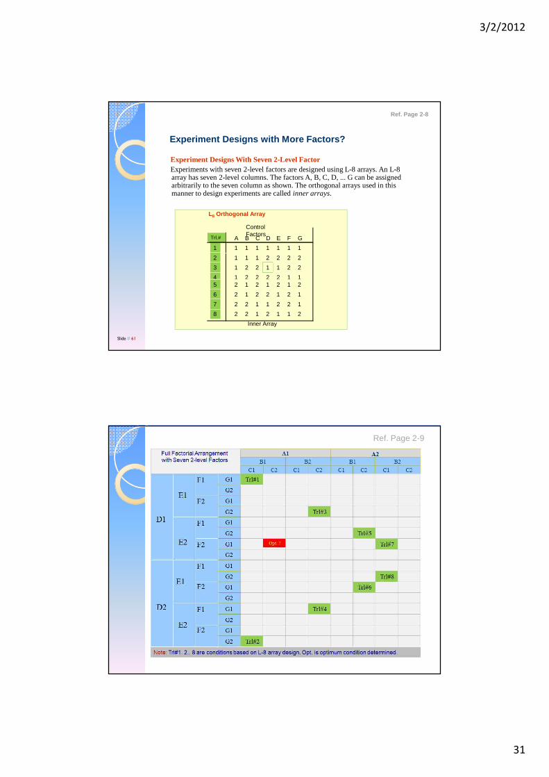
Experiment Designs With Seven 2-Level FactorExperiments with seven 2-level factors are designed using L-8 arrays. An L-8 array has seven 2-level columns. The factors A, B, C, D, ... G can be assigned arbitrarily to the seven column as shown. The orthogonal arrays used in this manner to design experiments are called inner arrays.
Experiment Designs with More Factors?
L8 Orthogonal Array
1
1
1
1
2
2
2
2
1
2
4
3
5
6
8
7
1
2
1
2
2
1
2
1
1
1
2
2
2
2
1
1
1
2
2
1
1
2
2
1
1
2
2
1
2
1
1
2
1
2
1
2
1
2
1
2
1
1
2
2
1
1
2
2
ETrl.# A CB FD G
Control Factors
Inner Array
Ref. Page 2-8
Slide # 61
Ref. Page 2-9
3/2/2012
32
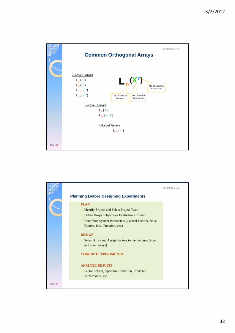
2-Level Arrays
L4 (23)
L8 (27)
L12 (211)
L16 (215)
3-Level Arrays
L9 (34)
L18 (21 37)
4-Level Arrays
L16 (45)
Common Orthogonal Arrays
L (XY)n
No. of rows in the array
No. of levels in the columns.
No. of columns in the array.
Ref. Page 2-10
Slide # 63
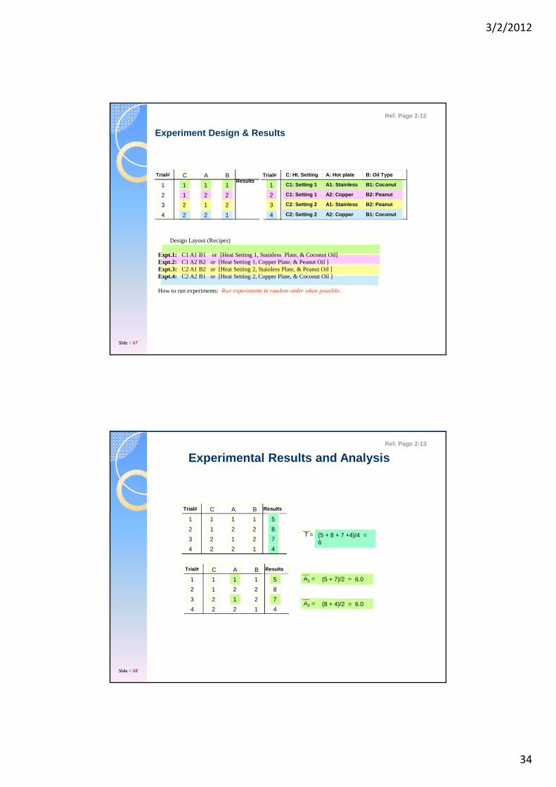
PLAN
� Identify Project and Select Project Team
� Define Project objectives Evaluation Criteria
� Determine System Parameters (Control Factors, Noise
Factors, Ideal Function, etc.)
DESIGN
� Select Array and Assign Factors to the columns (inner
and outer arrays)
CONDUCT EXPERIMENTS
ANALYZE RESULTS
� Factor Effects, Optimum Condition, Predicted
Performance, etc.
Planning Before Designing Experiments
Ref. Page 2-10
Slide # 64

3/2/2012
33
An ordinary kernel of corn, a little yellow seed, it just sits there. But add some oil, turn up the heat, and, pow. Within a second, an aromatic snack sensation has come into being: a fat, fluffy popcorn.
Note: C. Cretors & Company in the U.S. was the first company to develop popcorn machines, about 100 years ago.
Popcorn Machine Performance Study(Example Experiment)
This example is used to demonstrate “cradle to grave”, mini planning, design, and analyses tasks involved in DOE.
Ref. Page 2-11
Slide # 65
Project - Pop Corn Machine performance Study
Objective & Result- Determine best machine settings
Quality Characteristics- Measure unpopped kernels (Smalleris better)
Factors and Level Descriptions
Factor Level I Level II
A: Hot Plate Stainless Steel Copper Alloy
B: Type of Oil Coconut Oil Peanut Oil
C: Heat Setting Setting 1 Setting 2
Experiment Planning & Design
1
2
4
3
Trial# C: Ht. Setting A: Hot plate B: Oil Type
C1: Setting 1
C1: Setting 1
C2: Setting 2
C2: Setting 2
A1: Stainless
A2: Copper
A1: Stainless
A2: Copper
B1: Coconut
B2: Peanut
B2: Peanut
B1: Coconut
1
1
2
2
C A B
1
2
2
1
1
2
1
2
1
2
4
3
Trial#Results
Ref. Page 2-12
Slide # 66
3/2/2012
34
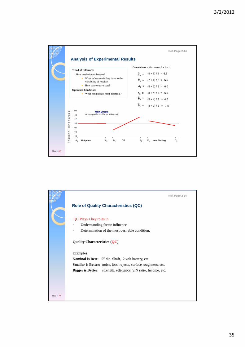
Experiment Design & Results
1
2
4
3
Trial# C: Ht. Setting A: Hot plate B: Oil Type
C1: Setting 1
C1: Setting 1
C2: Setting 2
C2: Setting 2
A1: Stainless
A2: Copper
A1: Stainless
A2: Copper
B1: Coconut
B2: Peanut
B2: Peanut
B1: Coconut
1
1
2
2
C A B
1
2
2
1
1
2
1
2
1
2
4
3
Trial#Results
Design Layout (Recipes)
Expt.1: C1 A1 B1 or [Heat Setting 1, Stainless Plate, & Coconut Oil]Expt.2: C1 A2 B2 or [Heat Setting 1, Copper Plate, & Peanut Oil ]Expt.3: C2 A1 B2 or [Heat Setting 2, Stainless Plate, & Peanut Oil ]Expt.4: C2 A2 B1 or [Heat Setting 2, Copper Plate, & Coconut Oil ]
How to run experiments: Run experiments in random order when possible.
Ref. Page 2-12
Slide # 67
Experimental Results and Analysis
A1 =__
(5 + 7)/2 = 6.0
1
1
2
2
C A B
1
2
2
1
1
2
1
2
1
2
4
3
Trial# Results
5
8
4
7
__T = (5 + 8 + 7 +4)/4 =
6
1
1
2
2
C A B
1
2
2
1
1
2
1
2
1
2
4
3
Trial# Results
5
8
4
7A2 =__
(8 + 4)/2 = 6.0
Ref. Page 2-13
Slide # 68
3/2/2012
35
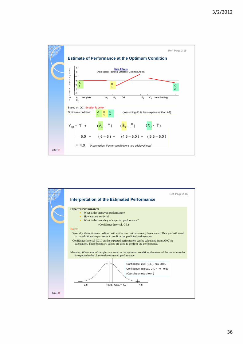
Trend of Influence:
How do the factor behave?
♦ What influence do they have to the variability of results?
♦ How can we save cost?
Optimum Condition:
♦ What condition is most desirable?
Calculations: ( Min. seven, 3 x 2 + 1)
(5 + 8) / 2 = 6.5
(7 + 4) / 2 = 5.5
(5 + 7) / 2 = 6.0
(8 + 4) / 2 = 6.0
(5 + 4) / 2 = 4.5
(8 + 7) / 2 = 7.5
_C2 =
_C1 =
_A2 =
_A1 =
_B1 = _B2 =
Analysis of Experimental Results
A1 Hot plate A2 B1 Oil B2 C1 Heat Setting C2
3
4
6
5
7
8
9UNPOPPED
KERNELS
Main Effects(Average effects of factor influence)
Ref. Page 2-14
Slide # 69
QC Plays a key roles in:
◦ Understanding factor influence
◦ Determination of the most desirable condition.
Quality Characteristics (QC)
Examples
Nominal is Best: 5” dia. Shaft,12 volt battery, etc.
Smaller is Better: noise, loss, rejects, surface roughness, etc.
Bigger is Better: strength, efficiency, S/N ratio, Income, etc.
Role of Quality Characteristics (QC)
Ref. Page 2-14
Slide # 70
3/2/2012
36
Estimate of Performance at the Optimum Condition
A1 Hot plate A2 B1 Oil B2 C1 Heat SettingC2
3
4
6
5
7
8
9UNPOPPED
KERNELS
Main Effects(Also called: Factorial Effects or Column Effects)
A1
B1 C
2
Based on QC: Smaller is better
Optimum condition: ( Assuming A1 is less expensive than A2)A1
B1
C2
= 6.0 + ( 6 – 6 ) + (4.5 – 6.0 ) + ( 5.5 – 6.0 )
= 4.0 (Assumption: Factor contributions are additive/linear)
_Yopt = T +
_( A1 -
_( C2 -
_T )
_( B1 -
_T )
_T )
Ref. Page 2-15
Slide # 71
Expected Performance:♦ What is the improved performance?♦ How can we verify it?♦ What is the boundary of expected performance?
(Confidence Interval, C.I.)
Notes:
Generally, the optimum condition will not be one that has already been tested. Thus you will need to run additional experiments to confirm the predicted performance.
Confidence Interval (C.I.) on the expected performance can be calculated from ANOVA calculation. These boundary values are used to confirm the performance.
Meaning: When a set of samples are tested at the optimum condition, the mean of the tested samples is expected to be close to the estimated performance.
Interpretation of the Estimated Performance
3.5 Yavg. Yexp. = 4.0 4.5
Confidence level (C.L.), say 90%.
Confidence Interval, C.I. = +/- 0.50
(Calculation not shown)
Ref. Page 2-16
Slide # 72
3/2/2012
37
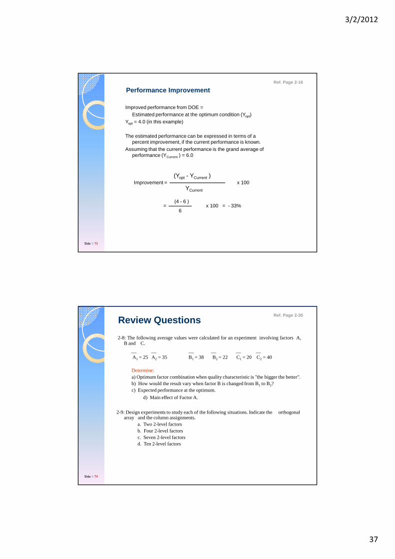
Performance Improvement
Improved performance from DOE = Estimated performance at the optimum condition (Yopt)
Yopt = 4.0 (in this example)
The estimated performance can be expressed in terms of a percent improvement, if the current performance is known.
Assuming that the current performance is the grand average of performance (YCurrent ) = 6.0
Improvement = x 100(Yopt - YCurrent )
YCurrent
= x 100 = - 33%(4 - 6 )
6
Ref. Page 2-16
Slide # 73
2-8: The following average values were calculated for an experiment involving factors A,B and C.
__ __ __ __ __ __A1 = 25 A2 = 35 B1 = 38 B2 = 22 C1 = 20 C2 = 40
Determine:a) Optimum factor combination when quality characteristicis "the bigger the better".b) How would the result vary when factor B is changed from B1 to B2?c) Expected performance at the optimum.
d) Main effect of Factor A.
2-9: Design experiments to study each of the following situations. Indicate the orthogonal array and the column assignments.
a. Two 2-level factorsb. Four 2-level factorsc. Seven 2-level factorsd. Ten 2-level factors
Review QuestionsRef. Page 2-35
Slide # 74
3/2/2012
38
SolveProblem 2A and 2B (30 minutes)
Recommendation: Solve problem as a group or solve individually and discuss with your TEAM member.
Note: Install Qualitek-4 software (if asked) using Reg.# 409240108100690. Remove software after class.
Ref. Page 2-42
Slide # 75
Practice and Learn
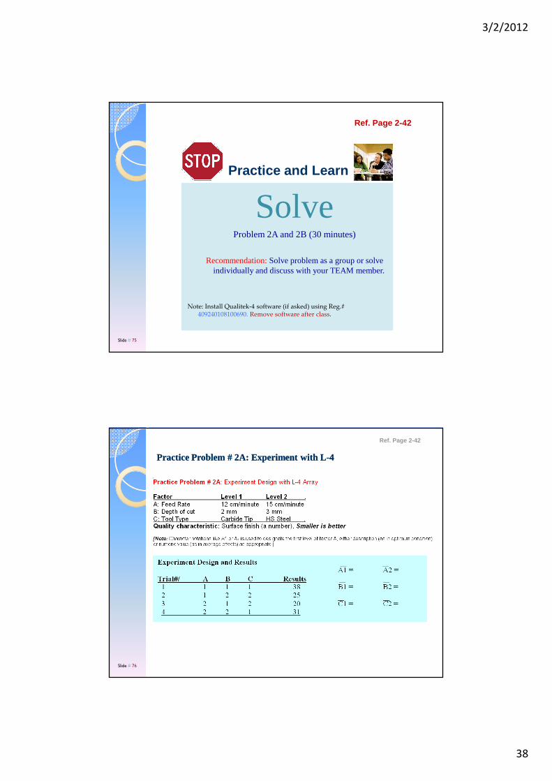
Practice Problem # 2A: Experiment with LPractice Problem # 2A: Experiment with L--44
Ref. Page 2-42
Slide # 76
3/2/2012
39
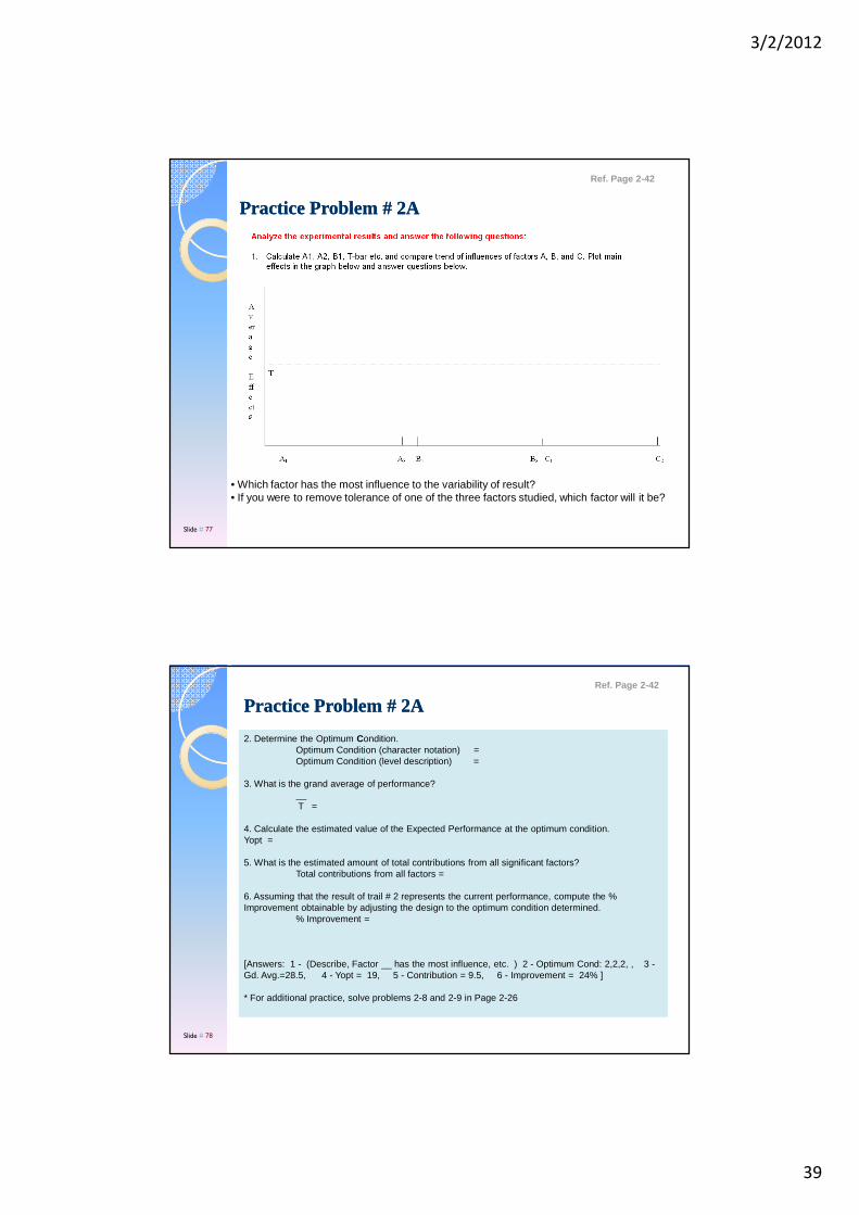
Practice Problem # 2APractice Problem # 2A
• Which factor has the most influence to the variability of result?• If you were to remove tolerance of one of the three factors studied, which factor will it be?
Ref. Page 2-42
Slide # 77
Practice Problem # 2APractice Problem # 2A
2. Determine the Optimum Condition. Optimum Condition (character notation) = Optimum Condition (level description) =
3. What is the grand average of performance?__T =
4. Calculate the estimated value of the Expected Performance at the optimum condition.Yopt =
5. What is the estimated amount of total contributions from all significant factors?Total contributions from all factors =
6. Assuming that the result of trail # 2 represents the current performance, compute the % Improvement obtainable by adjusting the design to the optimum condition determined.
% Improvement =
[Answers: 1 - (Describe, Factor __ has the most influence, etc. ) 2 - Optimum Cond: 2,2,2, , 3 -Gd. Avg.=28.5, 4 - Yopt = 19, 5 - Contribution = 9.5, 6 - Improvement = 24% ]
* For additional practice, solve problems 2-8 and 2-9 in Page 2-26
Ref. Page 2-42
Slide # 78
3/2/2012
40
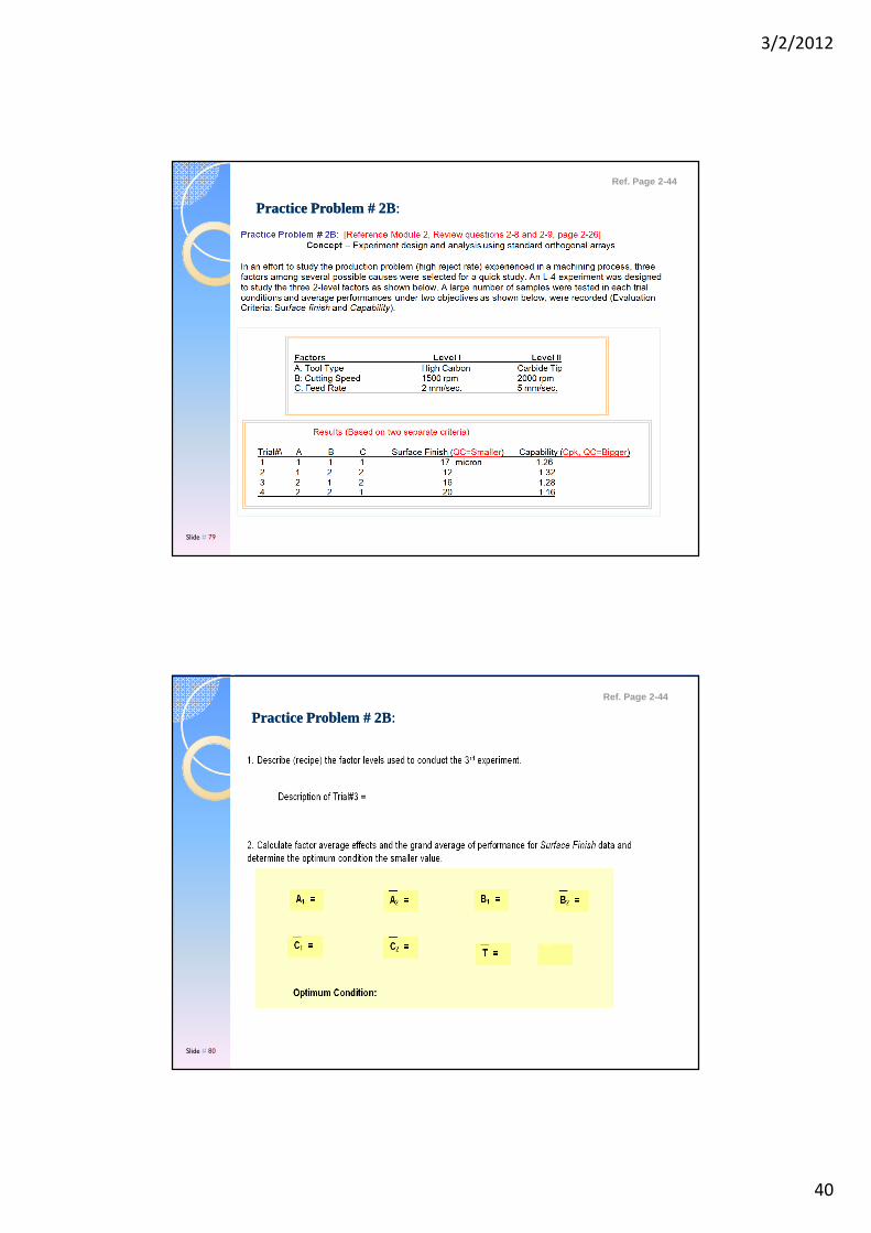
Practice Problem # 2BPractice Problem # 2B: :
Ref. Page 2-44
Slide # 79
Practice Problem # 2BPractice Problem # 2B: :
Ref. Page 2-44
Slide # 80
3/2/2012
41
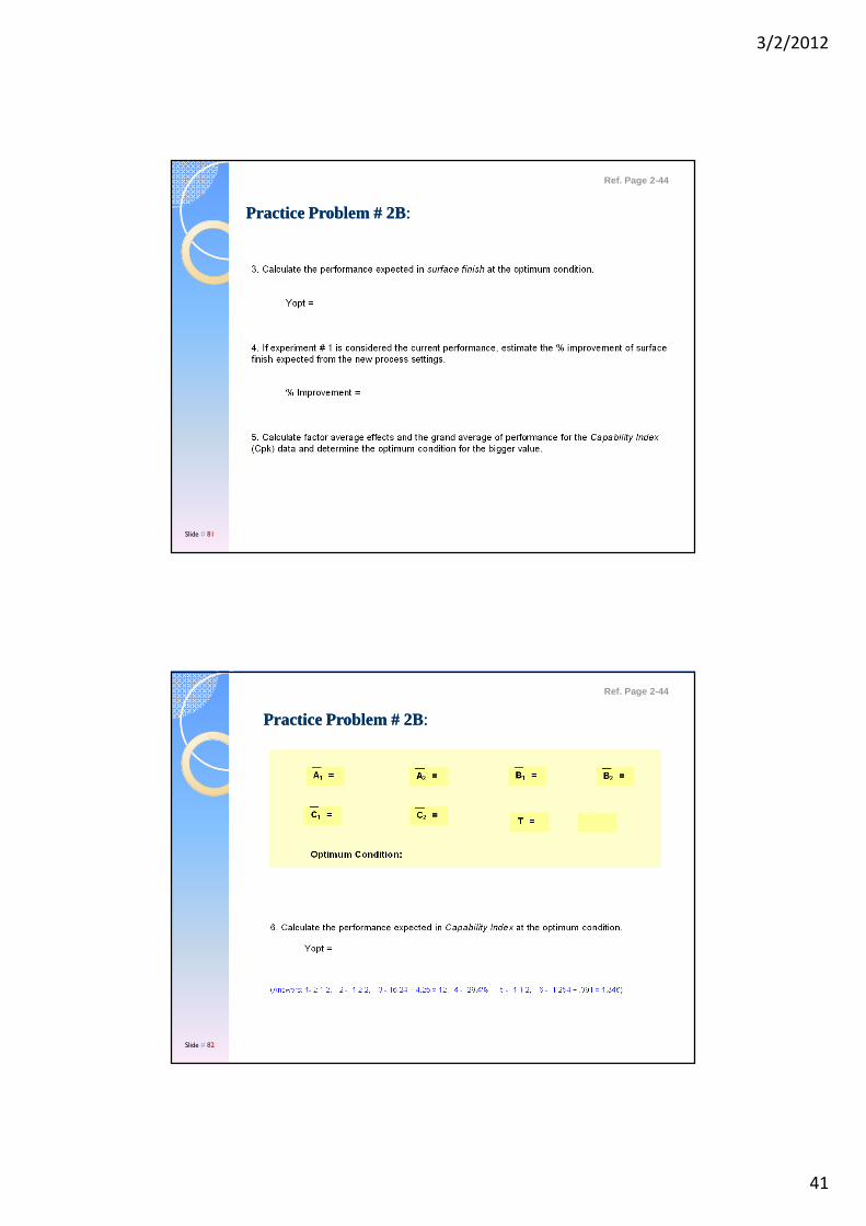
Practice Problem # 2BPractice Problem # 2B::
Ref. Page 2-44
Slide # 81
Practice Problem # 2BPractice Problem # 2B::
Ref. Page 2-44
Slide # 82
3/2/2012
42
Group Exercise Group Exercise -- Class ProjectClass Project
I. Experiment Planning
Project Title -
Objective & Result -
(Describe why you initiated the project and what you wish to accomplish)
Quality Characteristics: (Describe what you are after and how you would measure the results. Depending on what it is you are after, your quality characteristic will be bigger is better, smaller is better, or nominal is the best)
Factors and Level Descriptions
Notation/Factor Description Level I Level II
A:
B:
C: etc.
II. Experiment Design & Results
Our plan is to use _____ array. We/I want to complete design by assigning factors to the columns as.. Etc.
Slide # 83
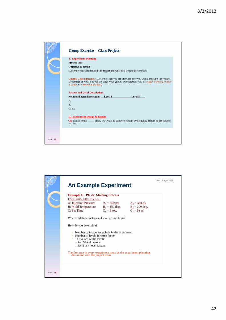
Example 1: Plastic Molding ProcessFACTORS and LEVELSA: Injection Pressure A1 = 250 psi A2 = 350 psiB: Mold Temperature B1 = 150 deg. B2 = 200 deg.C: Set Time C1 = 6 sec. C2 = 9 sec.
Where did these factors and levels come from?
How do you determine?
� Number of factors to include in the experiment� Number of levels for each factor� The values of the levels
- for 2-level factors- for 3 or 4-level factors
The first step in every experiment must be the experiment planning discussion with the project team.
An Example ExperimentRef. Page 2-16
Slide # 84
3/2/2012
43
Preparation for Planning Meeting
◦ Identify Project � One that gives “the biggest bang for the buck”.
◦ Form Team (3 – 12 people)� People with first hand knowledge� Internal customers� People responsible for implementation
◦ Schedule and convene an all-day experiment planning meeting with the team.� Inform and prepare all for a full day of meeting.
◦ As the project leader, invite all team members to attend the planning meeting. � Secure commitment to attend the meeting� Encourage team members to bring all project information to the meeting,
but discourage any formal research or documentations.� Study subject project and bring information with respect to details of
system breakdown (system into sub-systems, products into components) to the meeting.
Planning –The Essential First Step
Ref. Page 2-17
Slide # 85
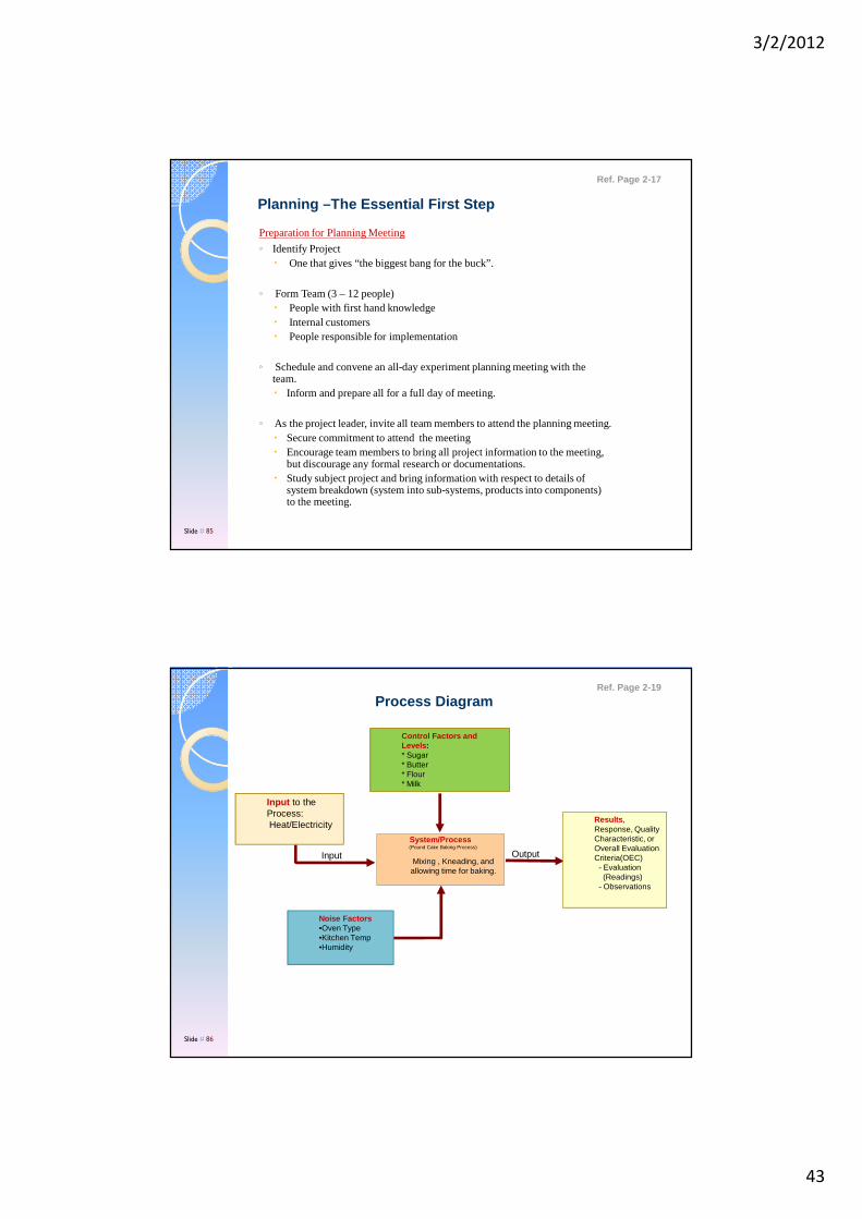
Process Diagram
Input
System/Process(Pound Cake Baking Process)
Mixing , Kneading, and allowing time for baking.
Output
Input to the Process:Heat/Electricity
Control Factors and Levels :* Sugar* Butter* Flour* Milk
Results , Response, Quality Characteristic, or Overall Evaluation Criteria(OEC)- Evaluation(Readings)
- Observations
Noise Factors•Oven Type•Kitchen Temp•Humidity
Ref. Page 2-19
Slide # 86

3/2/2012
44
Slide 87
Define SystemDefine SystemSystem may include all or part of the products or processes. It must always System may include all or part of the products or processes. It must always
include suspect areas (subinclude suspect areas (sub--processes or components) of the subject process processes or components) of the subject process under study. under study.
Slide # 87
Ref. Page N/A
Slide 88
System definition utilizes knowledge about problem and System definition utilizes knowledge about problem and probable causes.probable causes.
Consider the process of baking cakes (shown next).
Once the system is defined (boundaries), proceed to define:
- Outputs (Objectives)
- How outputs are measured- etc. (Planning discussions)
Ref. Page N/A
3/2/2012
45
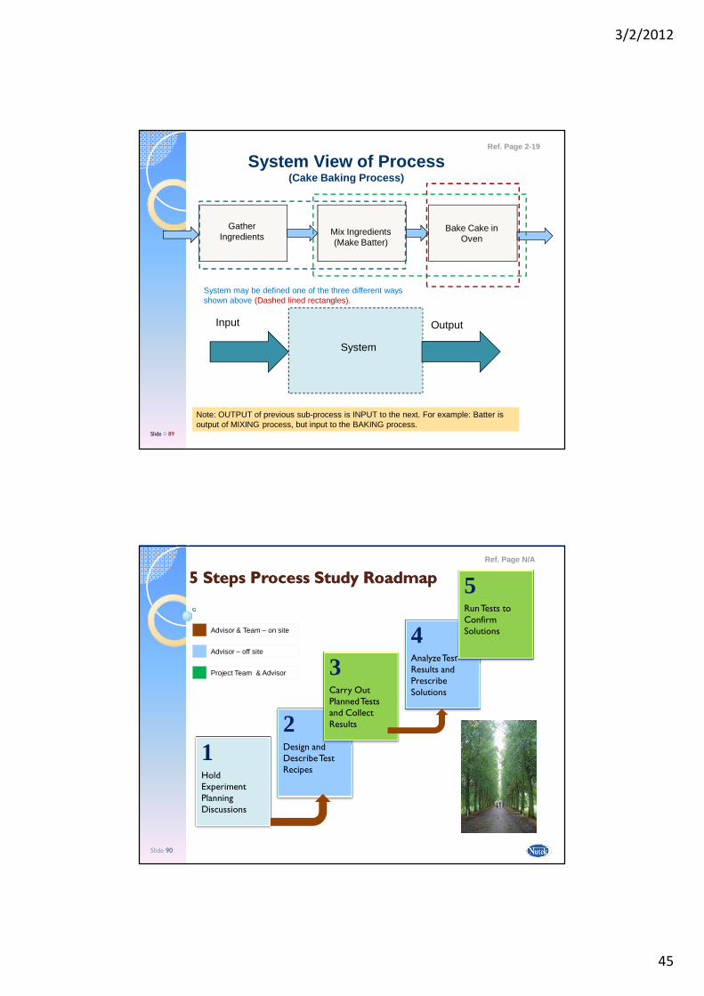
System View of Process(Cake Baking Process)
Ref. Page 2-19
Input Output
System
Note: OUTPUT of previous sub-process is INPUT to the next. For example: Batter is output of MIXING process, but input to the BAKING process.
Gather Ingredients Mix Ingredients
(Make Batter)
Bake Cake in Oven
System may be defined one of the three different ways shown above (Dashed lined rectangles).
Slide # 89
Slide 90
5 Steps Process Study Roadmap5 Steps Process Study Roadmap
1Hold Experiment Planning Discussions
2Design and Describe Test Recipes
4Analyze Test Results and Prescribe Solutions
3Carry Out Planned Tests and Collect Results
5Run Tests to Confirm SolutionsAdvisor & Team – on site
Advisor – off site
Project Team & Advisor
Ref. Page N/A
3/2/2012
46
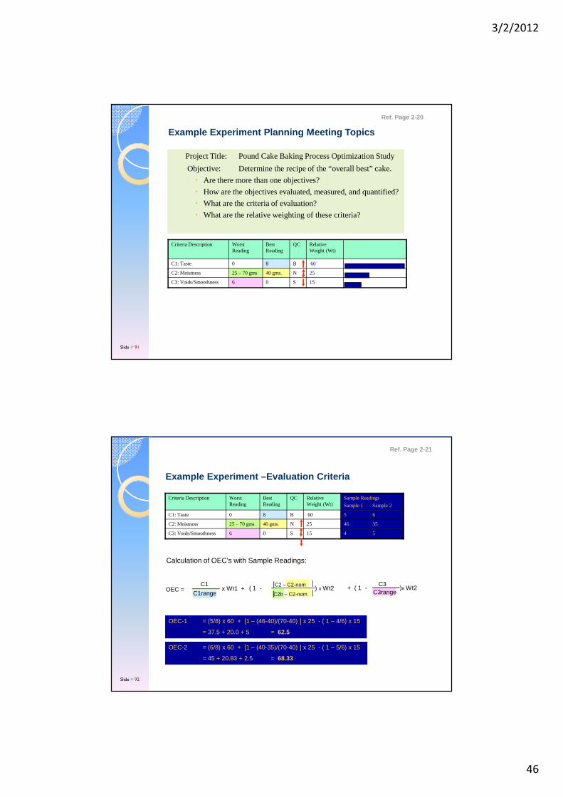
Example Experiment Planning Meeting Topics
Project Title: Pound Cake Baking Process Optimization Study
Objective: Determine the recipe of the “overall best” cake.
� Are there more than one objectives?
� How are the objectives evaluated, measured, and quantified?
� What are the criteria of evaluation?
� What are the relative weighting of these criteria?
Criteria Description Worst Reading
Best Reading
QC Relative Weight (Wt)
C1: Taste 0 8 B 60
C2: Moistness 25 – 70 gms 40 gms. N 25
C3: Voids/Smoothness 6 0 S 15
Ref. Page 2-20
Slide # 91
Example Experiment –Evaluation Criteria
Criteria Description Worst Reading
Best Reading
QC Relative Weight (Wt)
Sample Readings
Sample 1 Sample 2
C1: Taste 0 8 B 60 5 6
C2: Moistness 25 – 70 gms 40 gms. N 25 46 35
C3: Voids/Smoothness 6 0 S 15 4 5
OEC = C1
C1rangex Wt1 + ( 1 - ) x Wt2
C2b – C2-nom
C2 – C2-nom + ( 1 - )x Wt2 C3range
C3
OEC-1 = (5/8) x 60 + [1 – (46-40)/(70-40) ] x 25 - ( 1 – 4/6) x 15
= 37.5 + 20.0 + 5 = 62.5
OEC-2 = (6/8) x 60 + [1 – (40-35)/(70-40) ] x 25 - ( 1 – 5/6) x 15
= 45 + 20.83 + 2.5 = 68.33
Calculation of OEC’s with Sample Readings:
Ref. Page 2-21
Slide # 92
3/2/2012
47
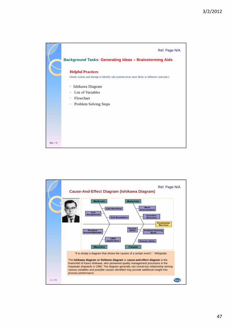
Helpful Practices(Study system and attempt to identify sub-systems/areas most likely to influence outcome.)
◦ Ishikawa Diagram
◦ List of Variables
◦ Flowchart
◦ Problem Solving Steps
Background Tasks: Generating Ideas – Brainstorming Aids
Ref. Page N/A
Slide # 93
Slide 94
Cause-And-Effect Diagram (Ishikawa Diagram)
“It is simply a diagram that shows the causes of a certain event.” - Wikipedia
The Ishikawa diagram or fishbone diagram or cause-and-effect diagram is the brainchild of Kaoru Ishikawa, who pioneered quality management processes in the Kawasaki shipyards in 1960. The diagram generally can reveal key relationship among various variables and possible causes identified may provide additional insight into process performance.
Ref. Page N/A
3/2/2012
48
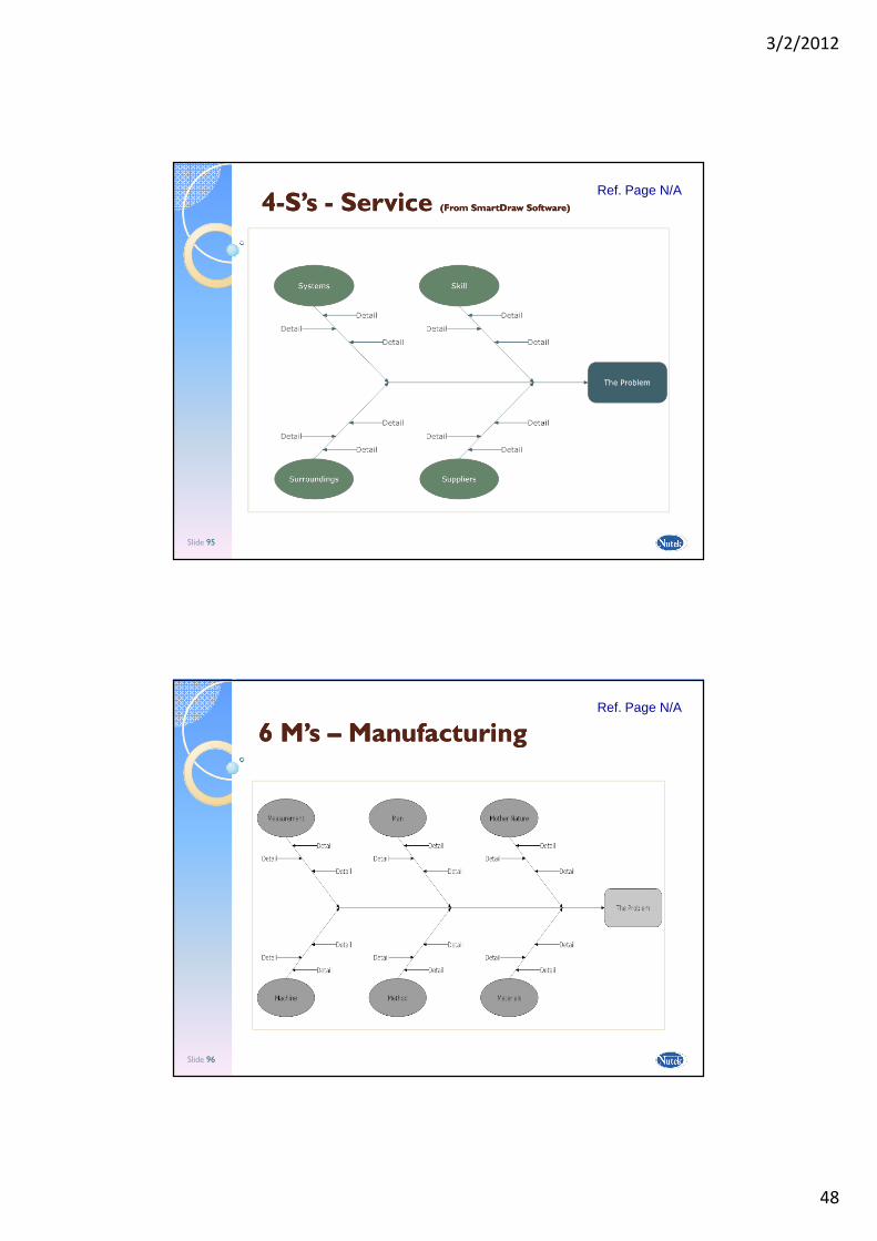
Slide 95
44--S’s S’s -- Service Service (From (From SmartDrawSmartDraw Software)Software)
Ref. Page N/A
Slide 96
6 M’s 6 M’s –– ManufacturingManufacturingRef. Page N/A
3/2/2012
49
Slide 97
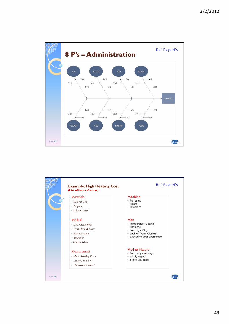
8 P’s 8 P’s –– AdministrationAdministrationRef. Page N/A
Slide 98
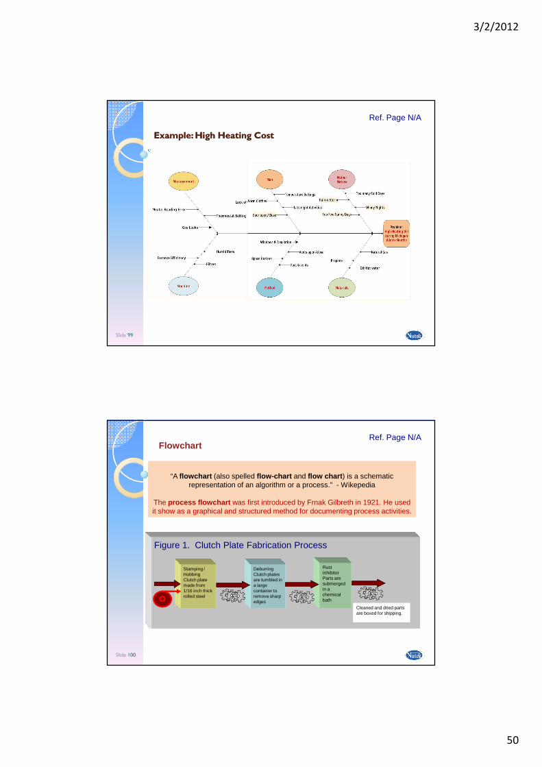
Materials• Natural Gas
• Propane
• Oil/Hot water
Method• Duct Cleanliness
• Vents Open & Close
• Space Heaters
• Insulation
• Window Glass
Measurement• Meter Reading Error
• Leaky Gas Tube
• Thermostat Control
Machine• Furnance• Filters• Himidifies
Man• Temperature Setting• Fireplace• Late night Stay• Lack of Worm Clothes• Excessive door open/close
Mother Nature• Too many clod days• Windy nights• Storm and Rain
Example: High Heating Cost Example: High Heating Cost (List of factors/causes)(List of factors/causes)
Ref. Page N/A
3/2/2012
50
Slide 99
Example: High Heating CostExample: High Heating Cost
Ref. Page N/A
Slide 100
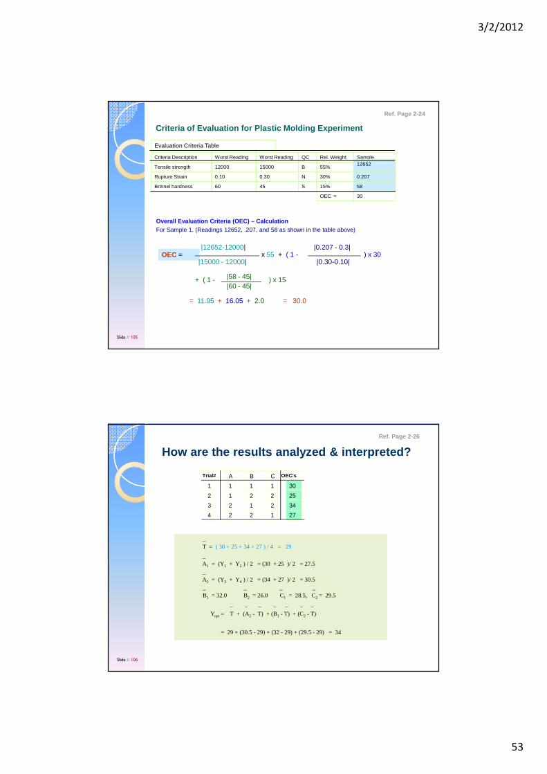
Flowchart
“A flowchart (also spelled flow-chart and flow chart ) is a schematic representation of an algorithm or a process.” - Wikepedia
The process flowchart was first introduced by Frnak Gilbreth in 1921. He used it show as a graphical and structured method for documenting process activities.
Figure 1. Clutch Plate Fabrication Process
Stamping /HobbingClutch plate made from 1/16 inch thick rolled steel
DeburringClutch plates are tumbled in a large container to remove sharp edges
Rust InhibitorParts are submerged in a chemical bath
Cleaned and dried parts are boxed for shipping.Cleaned and dried parts are boxed for shipping.
Ref. Page N/A

3/2/2012
51
Structured Steps tructured Steps tructured Steps tructured Steps (Use it when DOE is not applicable)(Use it when DOE is not applicable)(Use it when DOE is not applicable)(Use it when DOE is not applicable)
1.1.1.1. Form Team Form Team Form Team Form Team
2.2.2.2. Describe ProblemDescribe ProblemDescribe ProblemDescribe Problem
3.3.3.3. Contain ProblemContain ProblemContain ProblemContain Problem
4.4.4.4. Identify Root CausesIdentify Root CausesIdentify Root CausesIdentify Root Causes
5.5.5.5. Find SolutionsFind SolutionsFind SolutionsFind Solutions
6.6.6.6. Implement Permanent SolutionImplement Permanent SolutionImplement Permanent SolutionImplement Permanent Solution
7.7.7.7. Establish ControlsEstablish ControlsEstablish ControlsEstablish Controls
8.8.8.8. Recognize Team Recognize Team Recognize Team Recognize Team
Basic Disciplines of Problem Solving (8 D)
Ref. Page N/A
Factors Identification and Qualification (Planning)Factors Identification and Qualification (Planning)
Long List Qualified List Study List
1. Sugar
2. Butter
3. Sifted Cake Flour
4. Egg
5. Baking Powder…
6. Granulated Sugar
7. Vegetable Coloring
…….
12. Smell of Cake
13. Browning of cake
…
22. Type of Oven
23. Kitchen Temp.
24. Vanilla Extract
25. Brandy
26. Mixing Time
1. Sugar
2. Butter
3. Flour
4. Egg
5. Baking Powder…
6. Granulated Sugar
7. Vegetable Coloring
……….
12. Vanilla Extract
13. Brandy
===============
22. Type of Oven
23. Kitchen Temp.
Note: Scrutinize list to select factors (input variables)
Determine scopes of experiment (number of experiments possible based on time and money)
Suppose 8 -10 experiments.
Select L-8, which means 7 2-level factors can be studied.
Select 7 out of 13 factors by team consensus.
3
4
1
5
6
7
.
.
.
.
.
.
Ref. Page 2-22
Slide # 102

3/2/2012
52
Factors Level Identification Factors Level Identification –– Example ProjectExample Project
2-Level Factors 3- Level Factors 4- Level Factors
Select one level at left and one level at right of the current working condition.
Select two levels at either side of the current working condition, and the third level as the current working
condition.
Select two levels at the two extreme ends of the current working
condition and the other two between the two extremes.
1. Select level as far away as possible (extreme value) from the current working condition, but be sure to stay within working range.
2. Always select levels such that should it be identified as the optimum condition, it can be released immediately.
3. Because of the cost consequence, select two levels for the factorsunless it is a discrete factor or it is continuous factor with known nonlinearity.
Current Working Condition
X XCurrent Working
Condition
X XX XCurrent Working
Condition
X XX
Ref. Page 2-23
Slide # 103
Slide 104
Application Case Studies (Start Thinking about your own project)
- Team project- Dedicated planning meeting- Consensus decisions- etc.-
Ref. Page N/A
3/2/2012
53
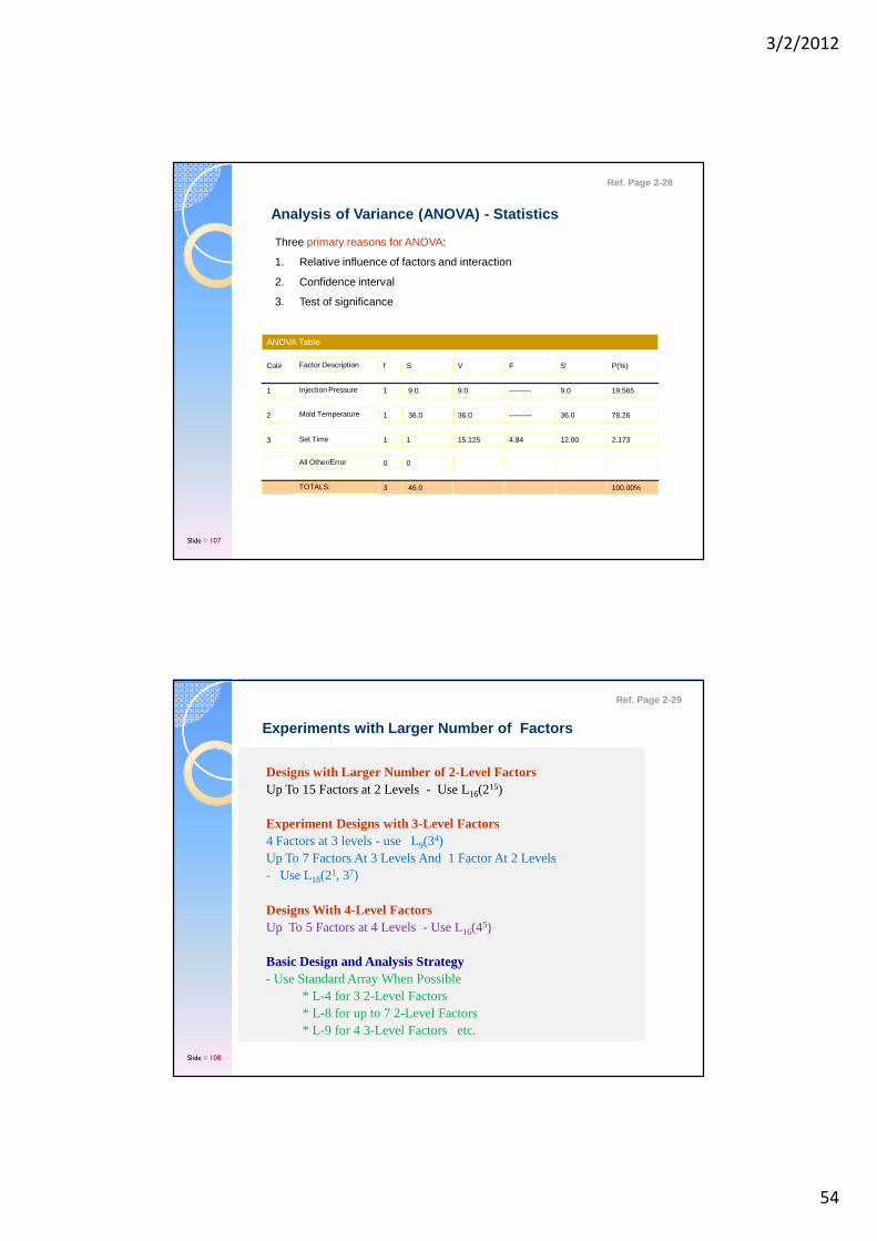
Overall Evaluation Criteria (OEC) – CalculationFor Sample 1. (Readings 12652, .207, and 58 as shown in the table above)
= 11.95 + 16.05 + 2.0 = 30.0
OEC = |12652-12000|
|15000 - 12000|x 55 + ( 1 - ) x 30
|0.207 - 0.3|
|0.30-0.10|
|58 - 45|+ ( 1 - ) x 15|60 - 45|
Criteria of Evaluation for Plastic Molding Experime nt
Evaluation Criteria Table
Criteria Description Worst Reading Worst Reading QC Rel. Weight Sample Reading
Tensile strength 12000 15000 B 55%12652
Brinnel hardness 60 45 S 15% 58
Rupture Strain 0.10 0.30 N 30% 0.207
OEC = 30
Ref. Page 2-24
Slide # 105
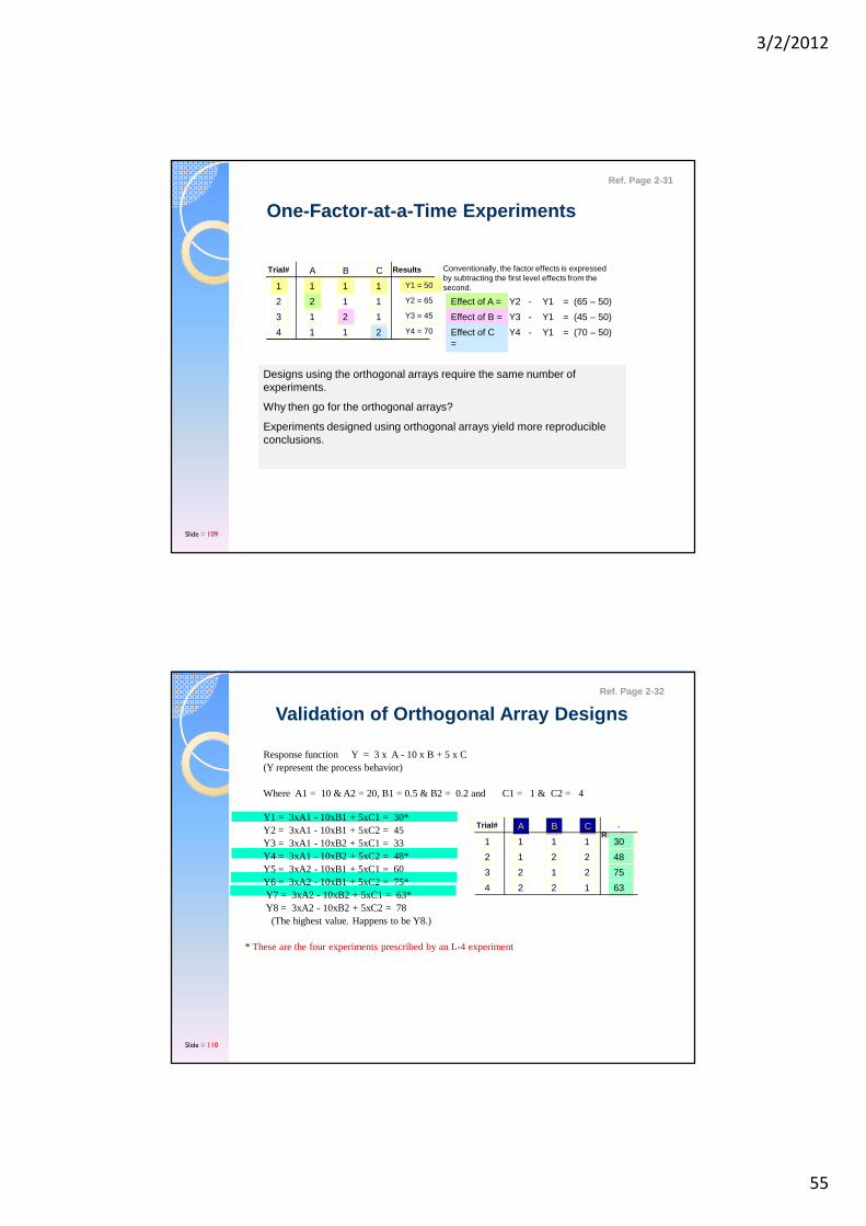
_T = ( 30 + 25 + 34 + 27 ) / 4 = 29
_A1 = (Y1 + Y2 ) / 2 = (30 + 25 )/ 2 = 27.5_A2 = (Y3 + Y4 ) / 2 = (34 + 27 )/ 2 = 30.5_ _ _ _B1 = 32.0 B2 = 26.0 C1 = 28.5, C2 = 29.5
_ _ _ _ _ _ _
Yopt = T + (A2 - T) + (B1 - T) + (C2 - T)
= 29 + (30.5 - 29) + (32 - 29) + (29.5 - 29) = 34
How are the results analyzed & interpreted?
1
1
2
2
A B C
1
2
2
1
1
2
1
2
1
2
4
3
Trial# OEC’s
30
25
27
34
Ref. Page 2-26
Slide # 106
3/2/2012
54
Three primary reasons for ANOVA:
1. Relative influence of factors and interaction
2. Confidence interval
3. Test of significance
Analysis of Variance (ANOVA) - Statistics
Col# Factor Description f S V F S’ P(%)
ANOVA Table
All Other/Error 0 0
3 Set Time 1 1 15.125 4.84 12.00 2.173
2 Mold Temperature 1 36.0 36.0 --------- 36.0 78.26
1 Injection Pressure 1 9.0 9.0 --------- 9.0 19.565
TOTALS: 3 46.0 100.00%
Ref. Page 2-28
Slide # 107
Designs with Larger Number of 2-Level FactorsUp To 15 Factors at 2 Levels - Use L16(215)
Experiment Designs with 3-Level Factors4 Factors at 3 levels - use L9(34)Up To 7 Factors At 3 Levels And 1 Factor At 2 Levels - Use L18(21, 37)
Designs With 4-Level FactorsUp To 5 Factors at 4 Levels - Use L16(45)
Basic Design and Analysis Strategy- Use Standard Array When Possible
* L-4 for 3 2-Level Factors* L-8 for up to 7 2-Level Factors* L-9 for 4 3-Level Factors etc.
Experiments with Larger Number of Factors
Ref. Page 2-29
Slide # 108
3/2/2012
55
Designs using the orthogonal arrays require the same number of experiments.
Why then go for the orthogonal arrays?
Experiments designed using orthogonal arrays yield more reproducible conclusions.
One-Factor-at-a-Time Experiments
1
2
1
1
A B C
1
1
1
2
1
1
2
1
1
2
4
3
Trial# Results
Y1 = 50
Y2 = 65
Y4 = 70
Y3 = 45
Effect of A = Y2 - Y1 = (65 – 50)
Effect of B = Y3 - Y1 = (45 – 50)
Effect of C =
Y4 - Y1 = (70 – 50)
Conventionally, the factor effects is expressed by subtracting the first level effects from the second.
Ref. Page 2-31
Slide # 109
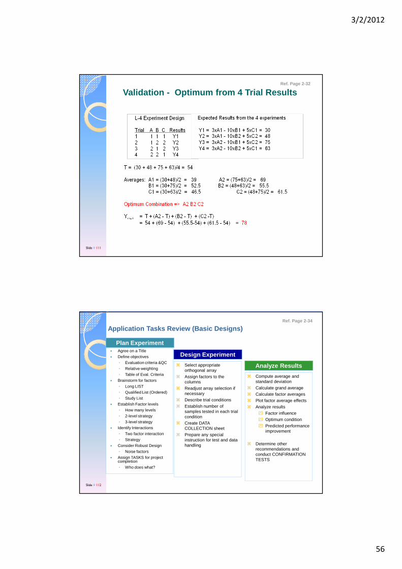
Validation of Orthogonal Array Designs
1
1
2
2
A B C
1
2
2
1
1
2
1
2
1
2
4
3
Trial#Results
30
48
63
75
Response function Y = 3 x A - 10 x B + 5 x C (Y represent the process behavior)
Where A1 = 10 & A2 = 20, B1 = 0.5 & B2 = 0.2 and C1 = 1 & C2 = 4
Y1 = 3xA1 - 10xB1 + 5xC1 = 30*Y2 = 3xA1 - 10xB1 + 5xC2 = 45Y3 = 3xA1 - 10xB2 + 5xC1 = 33Y4 = 3xA1 - 10xB2 + 5xC2 = 48*Y5 = 3xA2 - 10xB1 + 5xC1 = 60Y6 = 3xA2 - 10xB1 + 5xC2 = 75*Y7 = 3xA2 - 10xB2 + 5xC1 = 63*Y8 = 3xA2 - 10xB2 + 5xC2 = 78 (The highest value. Happens to be Y8.)
* These are the four experiments prescribed by an L-4 experiment
Ref. Page 2-32
Slide # 110
3/2/2012
56
Validation - Optimum from 4 Trial ResultsRef. Page 2-32
Slide # 111
Application Tasks Review (Basic Designs)
Plan Experiment� Agree on a Title
� Define objectives
◦ Evaluation criteria &QC
◦ Relative weighting
◦ Table of Eval. Criteria
� Brainstorm for factors
◦ Long LIST
◦ Qualified List (Ordered)
◦ Study List
� Establish Factor levels
◦ How many levels
◦ 2-level strategy
◦ 3-level strategy
� Identify Interactions
◦ Two factor interaction
◦ Strategy
� Consider Robust Design
◦ Noise factors
� Assign TASKS for project completion
◦ Who does what?
Design Experiment
� Select appropriate orthogonal array
� Assign factors to the columns
� Readjust array selection if necessary
� Describe trial conditions� Establish number of
samples tested in each trial condition
� Create DATA COLLECTION sheet
� Prepare any special instruction for test and data handling
Analyze Results
� Compute average and standard deviation
� Calculate grand average� Calculate factor averages� Plot factor average effects� Analyze results
Factor influence Optimum condition Predicted performance
improvement
� Determine other recommendations and conduct CONFIRMATION TESTS
Ref. Page 2-34
Slide # 112

3/2/2012
57
2-8: The following average values were calculated for an experiment involving factors A,B and C.
__ __ __ __ __ __A1 = 25 A2 = 35 B1 = 38 B2 = 22 C1 = 20 C2 = 40
Determine:a) Optimum factor combination when quality characteristicis "the bigger the better".b) How would the result vary when factor B is changed from B1 to B2?c) Expected performance at the optimum.
d) Main effect of Factor A.
2-9: Design experiments to study each of the following situations. Indicate the orthogonal array and the column assignments.
a. Two 2-level factorsb. Four 2-level factorsc. Seven 2-level factorsd. Ten 2-level factors
Review QuestionsRef. Page 2-35
Slide # 113
SolveProblem 2C and 2D (30 minutes)
Recommendation: Solve problem as a group or solve individually and discuss with your TEAM member.
Note: Install Qualitek-4 software (if asked) using Reg.# 409240108100690. Remove software after class.
Ref. Page 2-46
Slide # 114
Practice and Learn
3/2/2012
58
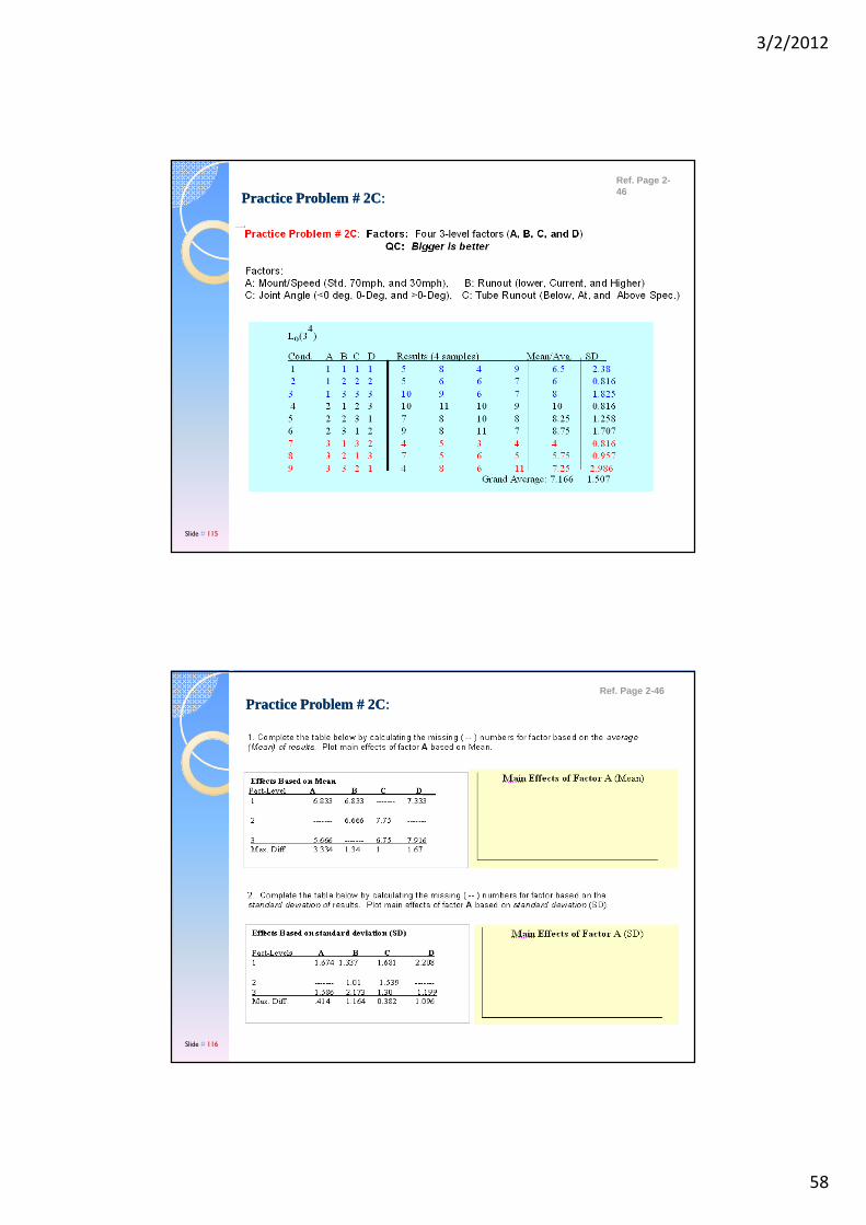
Practice Problem # 2CPractice Problem # 2C::Ref. Page 2-46
Slide # 115
Practice Problem # 2CPractice Problem # 2C::Ref. Page 2-46
Slide # 116
3/2/2012
59
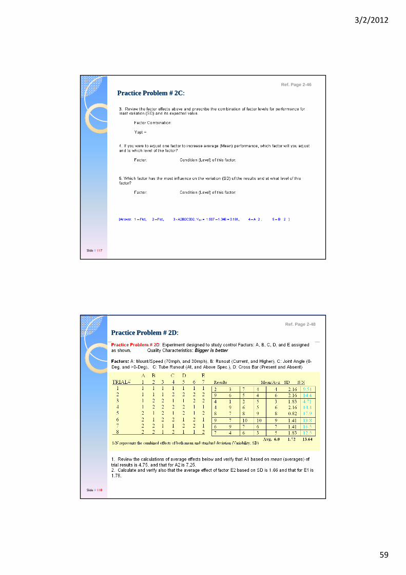
Practice Problem # 2CPractice Problem # 2C::Ref. Page 2-46
Slide # 117
Practice Problem # 2DPractice Problem # 2D::Ref. Page 2-48
Slide # 118
3/2/2012
60
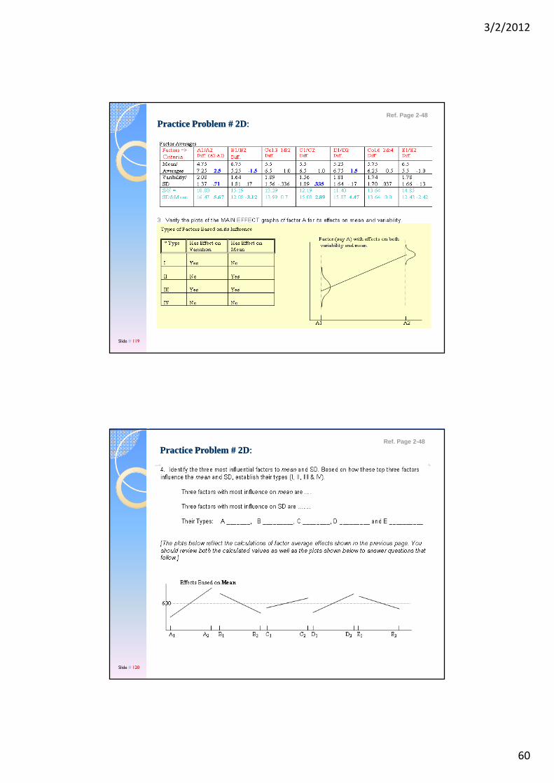
Practice Problem # 2DPractice Problem # 2D::Ref. Page 2-48
Slide # 119
Practice Problem # 2DPractice Problem # 2D::Ref. Page 2-48
Slide # 120

3/2/2012
61
Practice Problem # 2DPractice Problem # 2D::Ref. Page 2-49
Slide # 121
Practice Problem # 2DPractice Problem # 2D::Ref. Page 2-49
Slide # 122
3/2/2012
62
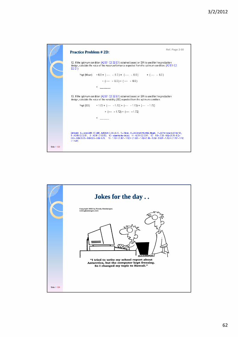
Practice Problem # 2DPractice Problem # 2D::Ref. Page 2-50
Slide # 123
Jokes for the day . .Jokes for the day . .
Slide # 124
3/2/2012
63
Module - 3Experiment Designs to Study Interactions
Slide # 125
Things you should learn from discussions in this module:
� What is interaction?
� Is interaction like a factor? Is it an input or an output?
� How many kinds of Interaction are there?
� Where does interactions show up?
� What can we do in our design to study interaction?
� How can you tell which interaction is stronger?
� When Interactions are too many, what is a good way to design the experiment?
Experiments to Study Interaction Between Factors
Ref. Pg. 3-1
Slide # 126
3/2/2012
64
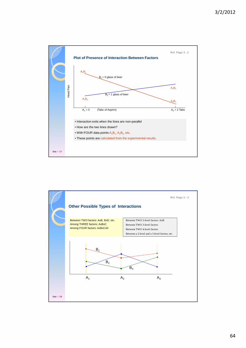
A1 = 0 (Tabs of Aspirin) A2 = 2 Tabs
Hea
d P
ain
B1 = 0 glass of beer
B2 = 1 glass of beer
A1B1
A2B1
A2B2
A1B2
• Interaction exits when the lines are non-parallel
• How are the two lines drawn?
• With FOUR data points A1B1, A1B2, etc.
• These points are calculated from the experimental results.
Plot of Presence of Interaction Between Factors
Ref. Page 3 - 2
Slide # 127
Between TWO 2-level factors: AxB
Between TWO 3-level factors
Between TWO 4-level factors
Between a 2-level and a 3-level factors, etc.
A1 A2 A3
B1
B2
B3
Other Possible Types of Interactions
Between TWO factors: AxB, BxD, etc.Among THREE factors: AxBxCAmong FOUR factors: AxBxCxD
Ref. Page 3 - 3
Slide # 128

3/2/2012
65
◦ Interaction effects can be theoretically determined from the array and the factor assignments. The task, however, is quite laborious. Fortunately, it has all been done by Taguchi.
◦ Reference: Pages 208 -212 QUALITY ENGINEERING by Yuin Wu and Dr. Willie Hobbs Moore
◦ Method: Interaction effect AxB (A in col 1, and B in col2 ) is the angle between the two lines which can be expressed in terms of results: Y, Y2, etc. This expression shows that it is the same for factor C in column 3.
Columns of Interaction Effects (AxB)
Ref. Page 3 - 5
Slide # 129
Number of Possible Factor Main Effects and Interaction Effects
Avg. Effect 2-factor 3-factor 4-factor 5-factor 6-factor 7-factor
1 7 21 35 35 21 7 1
(1 + 7 + 21 + 35 + 35 + 21 + 7 + 1) = 128
(27 = 128)
Calculation method: Two-Factor Interaction - two (say A and B) taken out of seven factors (The combination formula):
nCr = n!/[(n-r)! R! ] = 7 x 6 x 5! / [5!x 2 ] = 21
Ref: Page 374, STATISTICS FOR EXPERIMENTERS by Box, Hunter and Hunter
Scopes of Seminar: Learn how to study and make corrections for interactions between TWO 2-Level factors (AxB, BxC, etc)
Obtainable Information from Full-Factorial, 2 7 = 128
Ref. Page 3 - 5
Slide # 130
3/2/2012
66
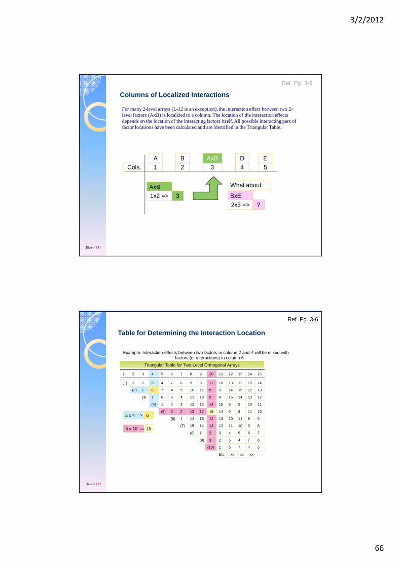
For many 2-level arrays (L-12 is an exception), the interaction effect between two 2-level factors (AxB) is localized to a column. The location of the interaction effects depends on the location of the interacting factors itself. All possible interacting pars of factor locations have been calculated and are identified in the Triangular Table.
Columns of Localized Interactions
A
1
B
2
AxB
3
AxB
1x2 => 3
D
4Cols.
BxE
2x5 => ?
E
5
What about
Ref. Pg. 3-6
Slide # 131
Table for Determining the Interaction Location
Example: Interaction effects between two factors in column 2 and 4 will be mixed with factors (or interactions) in column 6.
1 2 3 4 5 6 7 8 9 10 11 12 13 14 15
(1) 23 5 74 6 89 11 1310 12 1415
(2) 61 7 54 10 811 9 1514 12 13
(3) 67 5 114 10 89 15 1314 12
(4) 21 3 1312 14 815 9 1110
(5) 23 13 1512 14 89 11 10
(6) 141 15 1312 10 811 9
(7) 1415 13 1112 10 89
(8) 21 3 54 6 7
(9) 23 5 74 6
(10) 61 7 54
Etc. xxxx xx
2 x 4 => 6
5 x 10 => 15
Triangular Table for Two-Level Orthogonal Arrays
Ref. Pg. 3-6
Slide # 132
3/2/2012
67
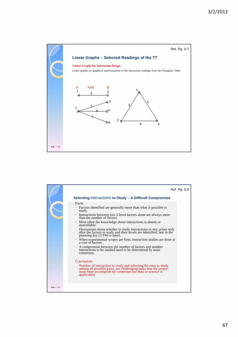
Linear Graphs for Interaction Design
Linear graphs are graphical representations of the interaction readings from the Triangular Table.
Linear Graphs – Selected Readings of the TT
13 2 1
2
3
46
5
1
2
345
6
7
A BAxB
Ref. Pg. 3-7
Slide # 133
Facts:◦ Factors identified are generally more than what is possible to
study.◦ Interactions between two 2-level factors alone are always more
than the number of factors.◦ Most often the knowledge about interactions is absent or
unavailable.◦ Discussions about whether to study interactions or not, arises only
after the factors to study and their levels are identified, late in the planning day (3 PM or later).
◦ When experimental scopes are firm, interaction studies are done at a cost of factors.
◦ A compromise between the number of factors and number interactions to be studied need to be determined by team consensus.
Conclusion:Number of interaction to study and selecting the ones to study among all possible pairs, are challenging tasks that the project team must accomplish by consensus (no data or science is applicable)
Selecting Interactions to Study – A Difficult Compromise
Ref. Pg. 3-8
Slide # 134
3/2/2012
68
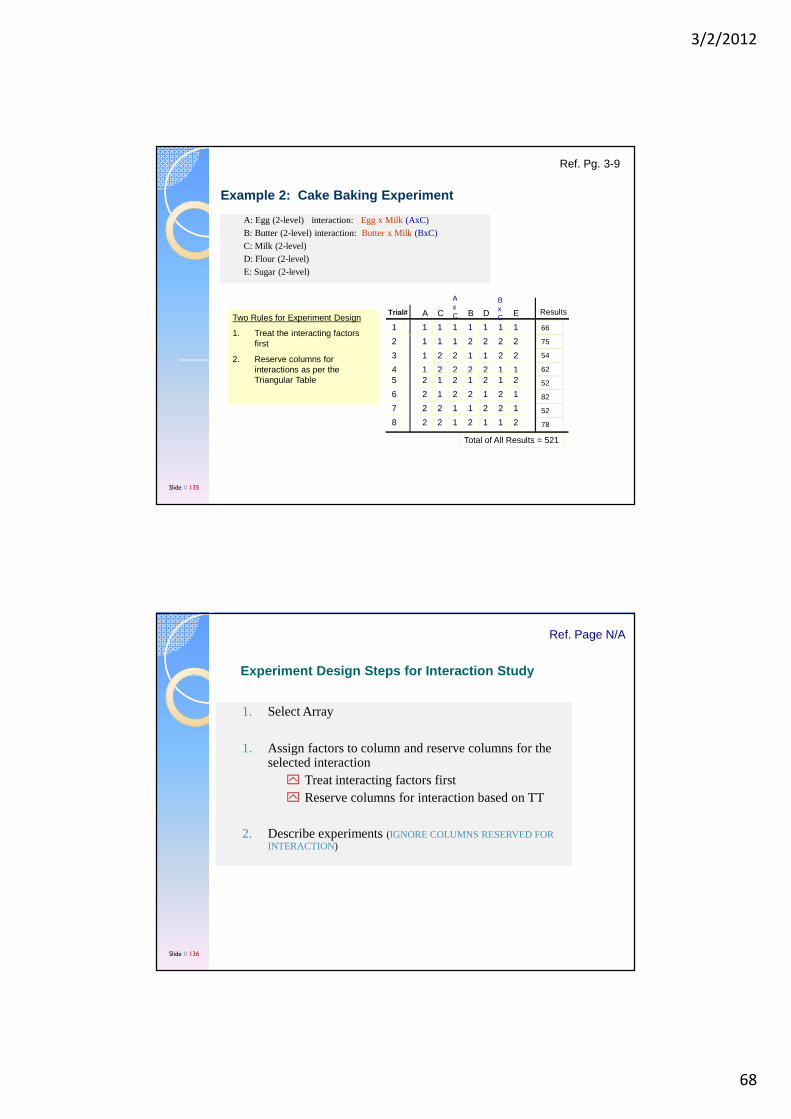
A: Egg (2-level) interaction: Egg x Milk (AxC)
B: Butter (2-level) interaction:Butter x Milk (BxC)
C: Milk (2-level)
D: Flour (2-level)
E: Sugar (2-level)
Example 2: Cake Baking Experiment
1
1
1
1
2
2
2
2
1
2
4
3
5
6
8
7
1
2
1
2
2
1
2
1
1
1
2
2
2
2
1
1
1
2
2
1
1
2
2
1
1
2
2
1
2
1
1
2
1
2
1
2
1
2
1
2
1
1
2
2
1
1
2
2
DTrial# A
AxCC
BxCB E Results
66
75
54
62
52
82
52
78
Total of All Results = 521
Two Rules for Experiment Design
1. Treat the interacting factors first
2. Reserve columns for interactions as per the Triangular Table
Ref. Pg. 3-9
Slide # 135
1. Select Array
1. Assign factors to column and reserve columns for the selected interaction
Treat interacting factors first Reserve columns for interaction based on TT
2. Describe experiments (IGNORE COLUMNS RESERVED FOR INTERACTION)
Experiment Design Steps for Interaction Study
Ref. Page N/A
Slide # 136
3/2/2012
69
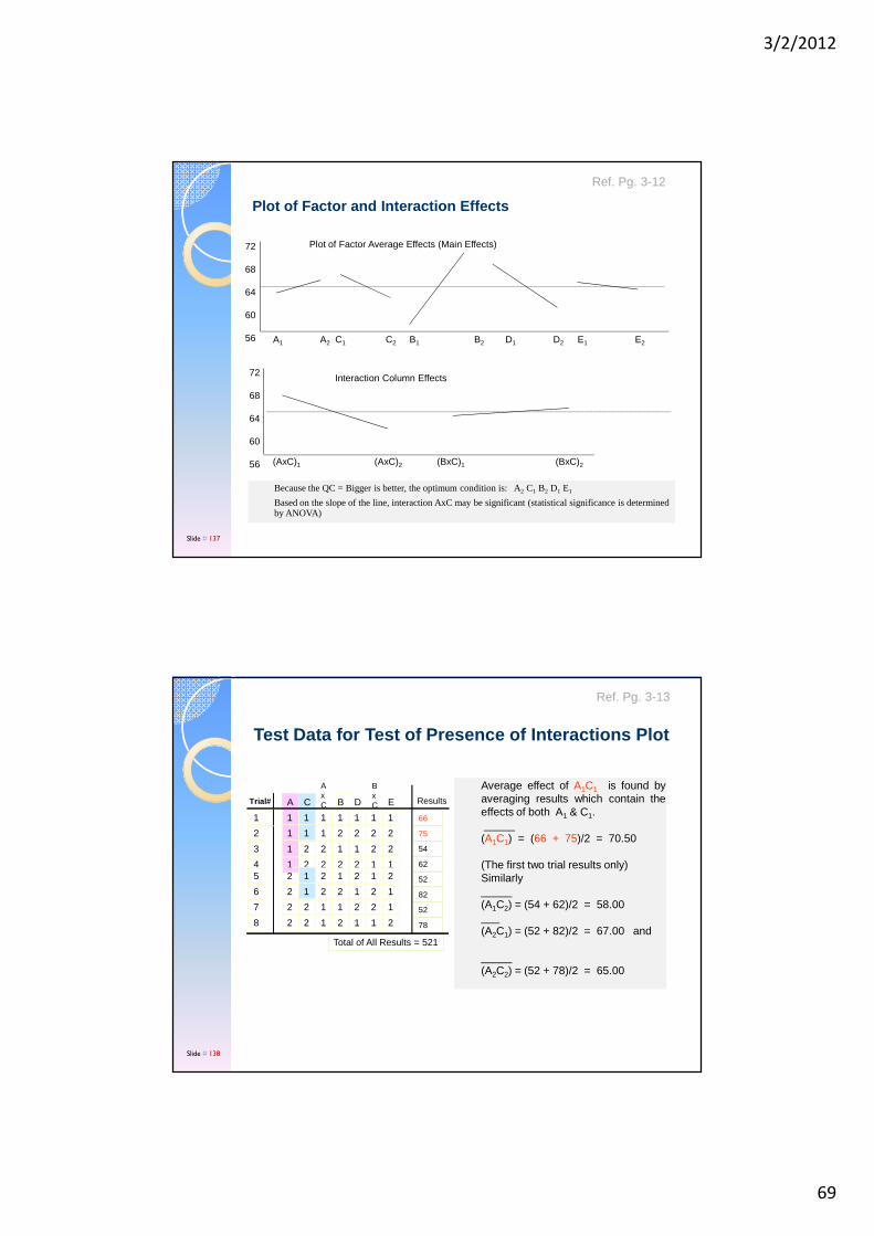
Because the QC = Bigger is better, the optimum condition is: A2 C1 B2 D1 E1
Based on the slope of the line, interaction AxC may be significant (statistical significance is determined by ANOVA)
A1 A2 C1 C2 B1 B2 D1 D2 E1 E2
72
68
64
60
56
Plot of Factor Average Effects (Main Effects)
Plot of Factor and Interaction Effects
(AxC)1 (AxC)2 (BxC)1 (BxC)2
72
68
64
60
56
Interaction Column Effects
Ref. Pg. 3-12
Slide # 137
Average effect of A1C1 is found byaveraging results which contain theeffects of both A1 & C1._____(A1C1) = (66 + 75)/2 = 70.50
(The first two trial results only)Similarly_____(A1C2) = (54 + 62)/2 = 58.00___(A2C1) = (52 + 82)/2 = 67.00 and
_____(A2C2) = (52 + 78)/2 = 65.00
Test Data for Test of Presence of Interactions Plot
1
1
1
1
2
2
2
2
1
2
4
3
5
6
8
7
1
2
1
2
2
1
2
1
1
1
2
2
2
2
1
1
1
2
2
1
1
2
2
1
1
2
2
1
2
1
1
2
1
2
1
2
1
2
1
2
1
1
2
2
1
1
2
2
DTrial# A
AxCC
BxCB E Results
66
75
54
62
52
82
52
78
Total of All Results = 521
Ref. Pg. 3-13
Slide # 138
3/2/2012
70
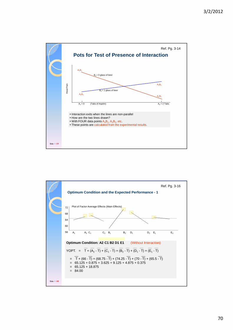
Pots for Test of Presence of Interaction
A1 = 0 (Tabs of Aspirin) A2 = 2 Tabs
Hea
d P
ain
B1 = 0 glass of beer
B2 = 1 glass of beer
A1B1
A2B1
A2B2
A1B2
• Interaction exits when the lines are non-parallel• How are the two lines drawn?• With FOUR data points A1B1, A1B2, etc.• These points are calculated from the experimental results.
Ref. Pg. 3-14
Slide # 139
Optimum Condition and the Expected Performance - 1
A1 A2 C1 C2 B1 B2 D1 D2 E1 E2
72
68
64
60
56
Plot of Factor Average Effects (Main Effects)
Optimum Condition: A2 C1 B2 D1 E1 (Without Interaction)__ __ __ __ __ __ __ __ __ __ __
YOPT. = T + (A2 - T) + (C1 - T) + (B2 - T) + (D1 - T) + (E1 - T)__ __ __ __ __ __
= T + (66 - T) + (68.75 - T) + (74.25 - T) + (70 - T) + (65.5 - T)= 65.125 + 0.875 + 3.625 + 9.125 + 4.875 + 0.375= 65.125 + 18.875 = 84.00
Ref. Pg. 3-16
Slide # 140
3/2/2012
71
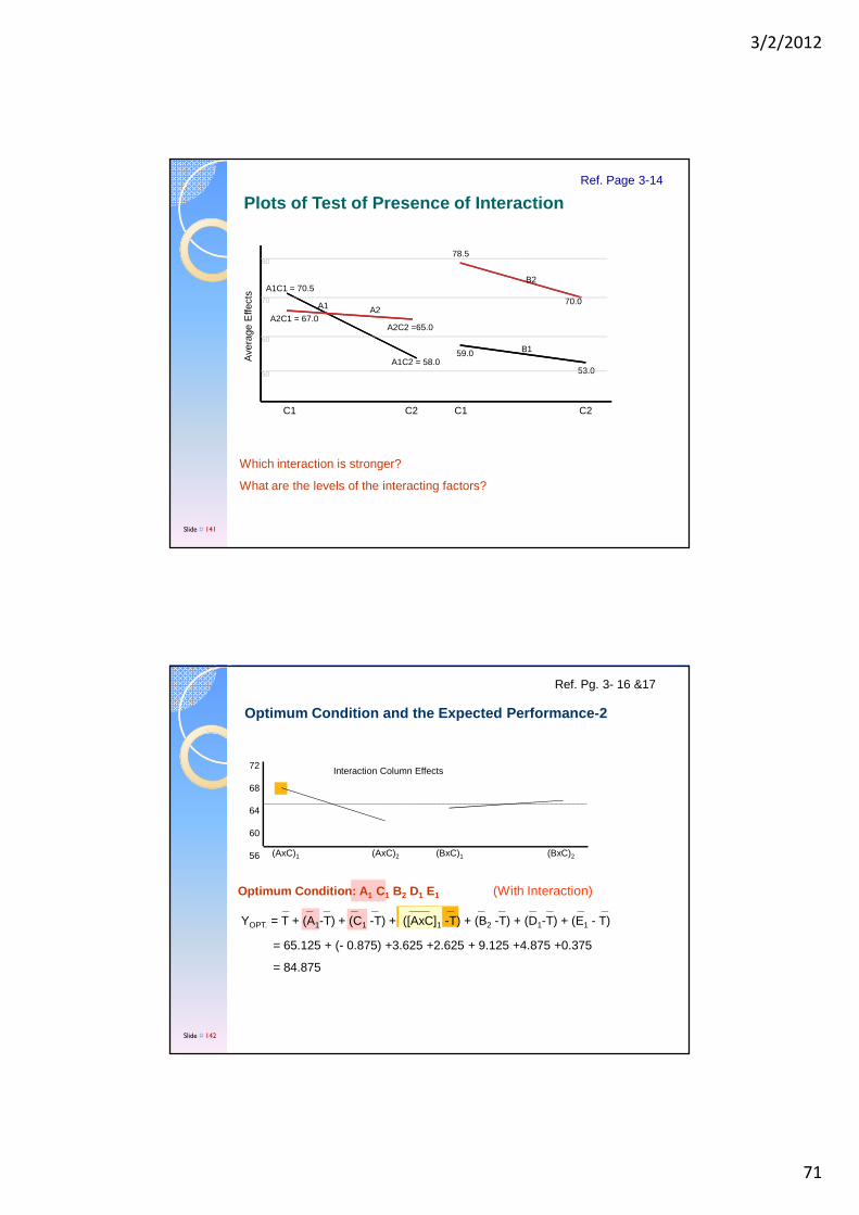
Plots of Test of Presence of InteractionRef. Page 3-14
Which interaction is stronger?
What are the levels of the interacting factors?
Slide # 141
A1C1 = 70.5
A1
A1C2 = 58.0
C1 C2 C1 C2
Ave
rage
Effe
cts
78.5
B2
70.0
B1
53.0
59.0
A2C1 = 67.0A2
A2C2 =65.0
80
70
60
50
Optimum Condition and the Expected Performance-2
(AxC)1 (AxC)2 (BxC)1 (BxC)2
72
68
64
60
56
Interaction Column Effects
Optimum Condition: A 1 C1 B2 D1 E1 (With Interaction)_ _ _ _ _ ___ _ _ _ _ _ _ _
YOPT. = T + (A1-T) + (C1 -T) + ([AxC]1 -T) + (B2 -T) + (D1-T) + (E1 - T)
= 65.125 + (- 0.875) +3.625 +2.625 + 9.125 +4.875 +0.375
= 84.875
Ref. Pg. 3- 16 &17
Slide # 142
3/2/2012
72
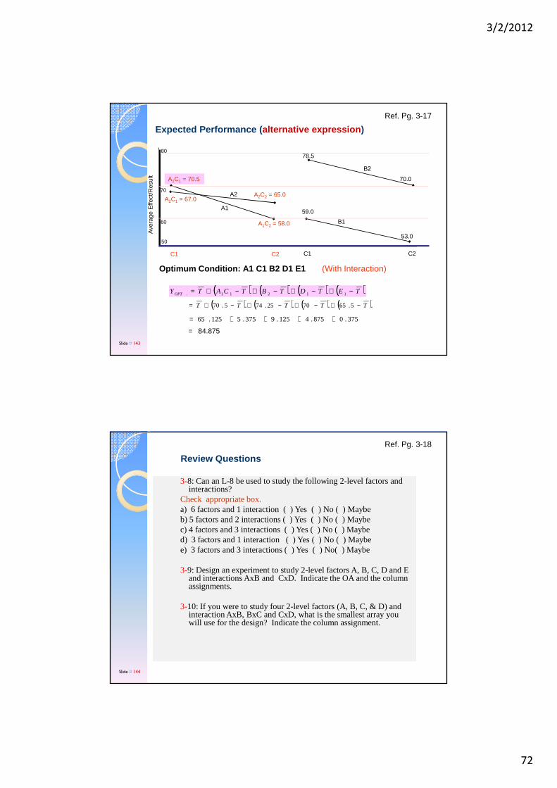
Expected Performance ( alternative expression )
( ) ( ) ( ) ( )TTTTT −+−+−+−+= 5.657025.745.70
375.0875.4125.9375.5125.65 ++++=
( ) ( ) ( ) ( )TETDTBTCATY OPT −+−+−+−+= 11211.
= 84.875
C1 C2 C1 C2
A1
A2
78.5
B1
70.0
59.0
53.0
80A
vera
ge E
ffect
/Res
ult
A1C1 = 70.5
A1C2 = 58.0
A2C1 = 67.0A2C2 = 65.0
60
70
50
Ref. Pg. 3-17
Optimum Condition: A1 C1 B2 D1 E1 (With Interaction)
Slide # 143
3-8: Can an L-8 be used to study the following 2-level factors and interactions?
Check appropriate box.a) 6 factors and 1 interaction ( ) Yes ( ) No ( ) Maybeb) 5 factors and 2 interactions ( ) Yes ( ) No ( ) Maybec) 4 factors and 3 interactions ( ) Yes ( ) No ( ) Maybed) 3 factors and 1 interaction ( ) Yes ( ) No ( ) Maybee) 3 factors and 3 interactions ( ) Yes ( ) No( ) Maybe
3-9: Design an experiment to study 2-level factors A, B, C, D and E and interactions AxB and CxD. Indicate the OA and the column assignments.
3-10: If you were to study four 2-level factors (A, B, C, & D) and interaction AxB, BxC and CxD, what is the smallest array you will use for the design? Indicate the column assignment.
Review Questions
Ref. Pg. 3-18
Slide # 144

3/2/2012
73
SolveProblem 3A, 3B and 3C (40 minutes)
Recommendation: Solve problem as a group or solve individually and discuss with your TEAM member.
Note: Install Qualitek-4 software (if asked) using Reg.# 409240108100690. Remove software after class.
Ref. Page 3-22
Slide # 145
Practice and Learn
Practice Problem # 3APractice Problem # 3A: : Rust Inhibitor Process StudyRust Inhibitor Process StudyQuality Characteristics: Quality Characteristics: Bigger is BetterBigger is Better
Ref. Pg. 3-22
Slide # 146
3/2/2012
74
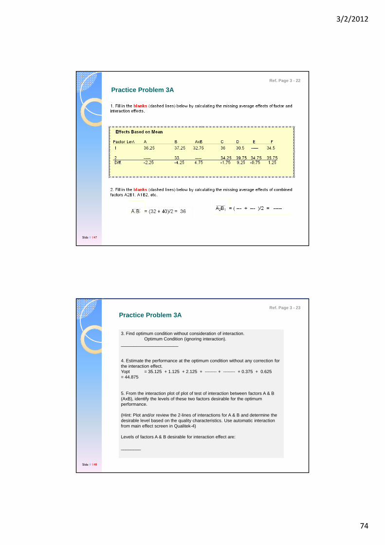
Practice Problem 3A
Ref. Page 3 - 22
Slide # 147
Practice Problem 3A
3. Find optimum condition without consideration of interaction.Optimum Condition (ignoring interaction).
_______________________
4. Estimate the performance at the optimum condition without any correction for the interaction effect.Yopt = 35.125 + 1.125 + 2.125 + -------- + -------- + 0.375 + 0.625 = 44.875
5. From the interaction plot of plot of test of interaction between factors A & B (AxB), identify the levels of these two factors desirable for the optimum performance.
(Hint: Plot and/or review the 2-lines of interactions for A & B and determine the desirable level based on the quality characteristics. Use automatic interaction from main effect screen in Qualitek-4)
Levels of factors A & B desirable for interaction effect are:
________
Ref. Page 3 - 23
Slide # 148
3/2/2012
75
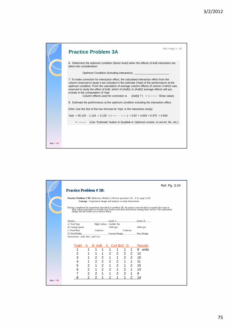
Practice Problem 3A
6. Determine the optimum condition (factor level) when the effects of AxB interaction are taken into consideration.
Optimum Condition (including interaction). _______________________
7. To make correction for interaction effect, the calculated interaction effect from the column reserved to study it are included in the estimate (Yopt) of the performance at the optimum condition. From the calculation of average column effects of column 3 which was reserved to study the effect of AxB, which of (AxB)1 or (AxB)2 average effects will you include in the computation of Yopt.
Column effects used for correction is (AxB)( ? ) = ( -------- Show value)
8: Estimate the performance at the optimum condition including the interaction effect.
(Hint: Use the first of the two formula for Yopt. in the interaction study)
Yopt = 35.125 - 1.125 + 2.125 + ( ----- - ------ ) + 0.87 + 4.625 + 0.375 + 0.625
= --------- (Use “Estimate” button in Qualitek-4, Optimum screen, to set A2, B1, etc.)
Ref. Page 3 - 23
Slide # 149
Practice Problem # 3BPractice Problem # 3B: :
Practice Problem # 3B: [Reference Module 3, Review questions 3-8 .. 3-11, page 3-16]Concept – Experiment design and analysis to study Interactions
Having completed the experiment described in problem 2B, the project team decided to expand the scope in their repeat experiment to include four Factors and three interactions among these factors. The experiment design and the results are as shown below.
Factors Level- I Level- IIA: Tool Type High Carbon Carbide TipB: Cutting Speed 1500 rpm 2000 rpmC: Feed Rate 2 mm/sec. 5 mm/sec.D: Tool Holder Current Design New DesignInteractions: AxB, BxC, and CxA
Trial# A B AxB C CxA BxC D Results1 1 1 1 1 1 1 1 8 units2 1 1 1 2 2 2 2 123 1 2 2 1 1 2 2 104 1 2 2 2 2 1 1 115 2 1 2 1 2 1 2 156 2 1 2 2 1 2 1 137 2 2 1 1 2 2 1 98 2 2 1 2 1 1 2 14
Ref. Pg. 3-24
Slide # 150
3/2/2012
76
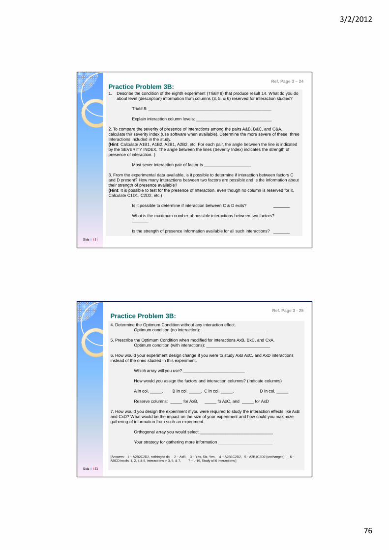
Practice Problem 3B:1. Describe the condition of the eighth experiment (Trial# 8) that produce result 14. What do you do
about level (description) information from columns (3, 5, & 6) reserved for interaction studies?
Trial# 8: ____________________________________________________
Explain interaction column levels: ________________________________
2. To compare the severity of presence of interactions among the pairs A&B, B&C, and C&A, calculate thir severity index (use software when available). Determine the more severe of these three Interactions included in the study.(Hint : Calculate A1B1, A1B2, A2B1, A2B2, etc. For each pair, the angle between the line is indicated by the SEVERITY INDEX. The angle between the lines (Severity Index) indicates the strength of presence of interaction. )
Most sever interaction pair of factor is ____________________
3. From the experimental data available, is it possible to determine if interaction between factors C and D present? How many interactions between two factors are possible and is the information about their strength of presence available?(Hint : It is possible to test for the presence of Interaction, even though no column is reserved for it. Calculate C1D1, C2D2, etc.)
Is it possible to determine if interaction between C & D exits? _______
What is the maximum number of possible interactions between two factors? _______
Is the strength of presence information available for all such interactions? _______
Ref. Page 3 – 24
Slide # 151
Practice Problem 3B:4. Determine the Optimum Condition without any interaction effect.
Optimum condition (no interaction): ___________________________
5. Prescribe the Optimum Condition when modified for interactions AxB, BxC, and CxA.Optimum condition (with interactions): ___________________________
6. How would your experiment design change if you were to study AxB AxC, and AxD interactions instead of the ones studied in this experiment.
Which array will you use? __________________________
How would you assign the factors and interaction columns? (Indicate columns)
A in col. _____, B in col. _____, C in col. _____, D in col. _____
Reserve columns: _____ for AxB, _____ fo AxC, and _____ for AxD
7. How would you design the experiment if you were required to study the interaction effects like AxBand CxD? What would be the impact on the size of your experiment and how could you maximize gathering of information from such an experiment.
Orthogonal array you would select _______________________________
Your strategy for gathering more information _______________________
[Answers: 1 – A2B2C2D2, nothing to do, 2 – AxB, 3 – Yes, Six, Yes, 4 – A2B1C2D2, 5 - A2B1C2D2 (unchanged), 6 –ABCD incols. 1, 2, 4 & 6, interactions in 3, 5, & 7, 7 – L-16, Study all 6 interactions ]
Ref. Page 3 - 25
Slide # 152

3/2/2012
77
Practice Problem # 3C
Ref. Pg. 3-26
Slide # 153
Ref. Page 3-26
Your group will be asked to discuss one or all of the following:
1. Evaluation criteria, their ranges of evaluations, QC, and their relative weighting (create the OEC table with assumed ranges of evaluations.Skip questions 1 - 3 if you have only one objective.)
Slide # 154

3/2/2012
78
Practice Problem # 3DPractice Problem # 3D: (Optional Exercise): (Optional Exercise)
Optimize Paper Helicopter Design Shown
Lower Body
Wing
Upper Body
WingAssignment:
(I) Practice making a few helicopters and fly them,
(II) Brainstorm and select factors (A, B, C, D, etc.) and determine the two levels for each factor. Design an experiment and construct eight helicopters. Fly your models and collect three flight duration (# of rotation or time) data under each of the two noise levels. Analyze results and confirm the optimum design.
(Do this project as a group when time permits)
Ref. Page 3-28
Slide # 155
Steps:
1. Make a few sample helicopters and practice flying it
2. Define factors (5 factors) and establish levels (2 levels, keep length/width ratio between 3 to 5)
3. Design experiments:1. Select array (L-18)2. Assign factors to columns3. Describe experiments (8 trial conditions)
4. Make Helicopters (8 separate designs) and identify them
5. Fly helicopters and collect FLIGHT TIME data (3 – 5 samples in each trial)
6. Analyze results 1. Find optimum designs2. Estimate optimum performance
7. Make a helicopter in optimum design
8. Run confirmation flights
9. Compare confirmation test results with prediction
Paper Helicopter Design Optimization WorkshopRef. Page N/A
Slide # 156

3/2/2012
79
Module - 4Experiment Designs with Mixed-Level Factors
Slide # 157
Things you should learn from discussions in this module:
� How standard orthogonal arrays are modified to use it for many experiment designs with mixed level factors.
� What is degrees of freedom (DOF)?
� How to determine requirements for the experiment in terms of DOF?
� How to determine which array is most suitable for modification?
� How to upgrade columns?
� How to downgrade columns?
� What is a combination design?
Designing Experiments with Mixed Factor Levels
Ref. Pg. 4-1
Slide # 158
3/2/2012
80
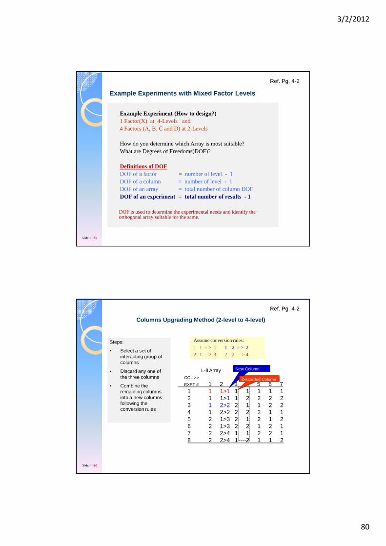
Example Experiment (How to design?)1 Factor(X) at 4-Levels and 4 Factors (A, B, C and D) at 2-Levels
How do you determine which Array is most suitable?What are Degrees of Freedoms(DOF)?
Definitions of DOFDOF of a factor = number of level - 1DOF of a column = number of level - 1DOF of an array = total number of column DOFDOF of an experiment = total number of results - 1
DOF is used to determine the experimental needs and identify the orthogonal array suitable for the same.
Example Experiments with Mixed Factor Levels
Ref. Pg. 4-2
Slide # 159
Assume conversion rules:
1 1 = > 1 1 2 = > 2
2 1 = > 3 2 2 = > 4
L-8 ArrayCOL >>
EXPT # 1 2 3 4 5 6 71 1 1>1 1 1 1 1 12 1 1>1 1 2 2 2 23 1 2>2 2 1 1 2 24 1 2>2 2 2 2 1 15 2 1>3 2 1 2 1 26 2 1>3 2 2 1 2 17 2 2>4 1 1 2 2 18 2 2>4 1 2 1 1 2
New Column
Discarded Column
Columns Upgrading Method (2-level to 4-level)
Steps:
• Select a set of interacting group of columns
• Discard any one of the three columns
• Combine the remaining columns into a new columns following the conversion rules
Ref. Pg. 4-2
Slide # 160
3/2/2012
81
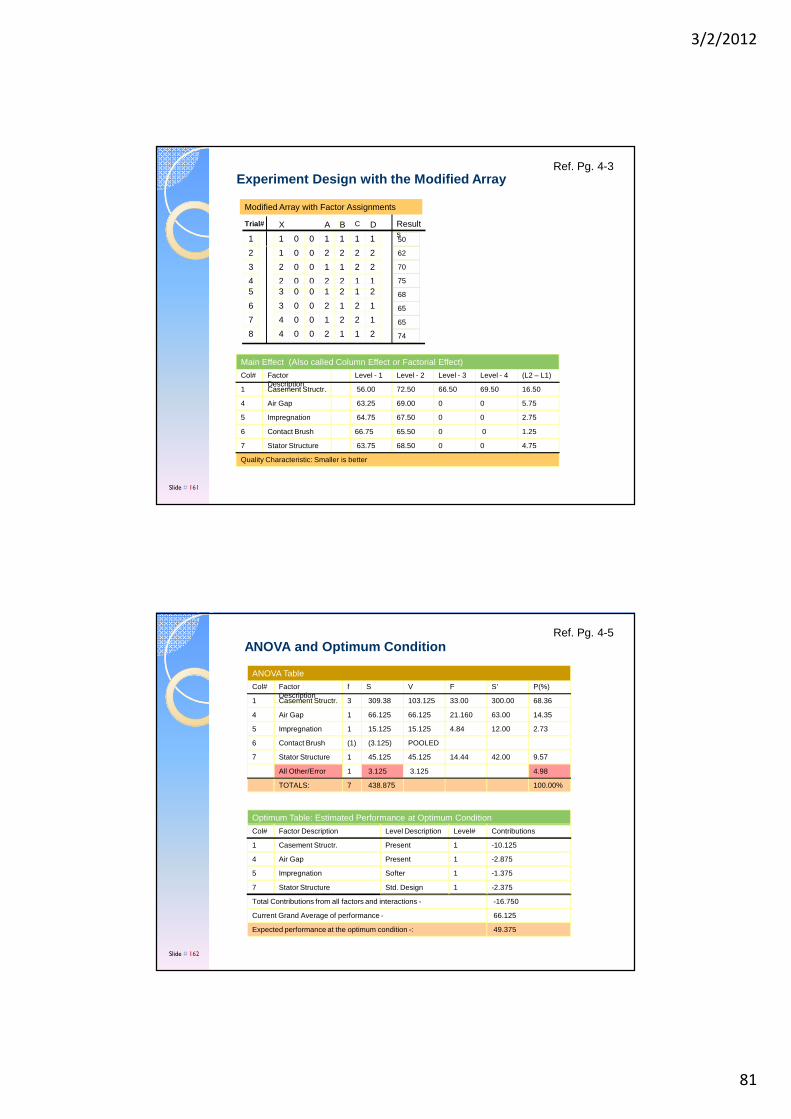
Experiment Design with the Modified Array
Col# Factor Description
Level - 1 Level - 2 Level - 3 Level - 4 (L2 – L1)
Main Effect (Also called Column Effect or Factorial Effect)
7 Stator Structure 63.75 68.50 0 0 4.75
6 Contact Brush 66.75 65.50 0 0 1.25
5 Impregnation 64.75 67.50 0 0 2.75
4 Air Gap 63.25 69.00 0 0 5.75
1 Casement Structr. 56.00 72.50 66.50 69.50 16.50
Quality Characteristic: Smaller is better
1
1
2
2
3
3
4
4
1
2
4
3
5
6
8
7
1
2
1
2
2
1
2
1
0
0
0
0
0
0
0
0
1
2
2
1
1
2
2
1
1
2
2
1
2
1
1
2
1
2
1
2
1
2
1
2
0
0
0
0
0
0
0
0
BTrial# X CA D Results50
62
70
75
68
65
65
74
Modified Array with Factor Assignments
Ref. Pg. 4-3
Slide # 161
ANOVA and Optimum Condition
Optimum Table: Estimated Performance at Optimum Condition
7 Stator Structure
5 Impregnation
4 Air Gap
1 Casement Structr.
Total Contributions from all factors and interactions - -16.750
Col# Factor Description Level Description Level# Contributions
Std. Design 1 -2.375
Present 1 -2.875
Present 1 -10.125
Softer 1 -1.375
Expected performance at the optimum condition -: 49.375
Current Grand Average of performance - 66.125
Col# Factor Description
f S V F S’ P(%)
ANOVA Table
7 Stator Structure 1 45.125 45.125 14.44 42.00 9.57
All Other/Error 1 3.125 3.125 4.98
6 Contact Brush (1) (3.125) POOLED
5 Impregnation 1 15.125 15.125 4.84 12.00 2.73
4 Air Gap 1 66.125 66.125 21.160 63.00 14.35
1 Casement Structr. 3 309.38 103.125 33.00 300.00 68.36
TOTALS: 7 438.875 100.00%
Ref. Pg. 4-5
Slide # 162
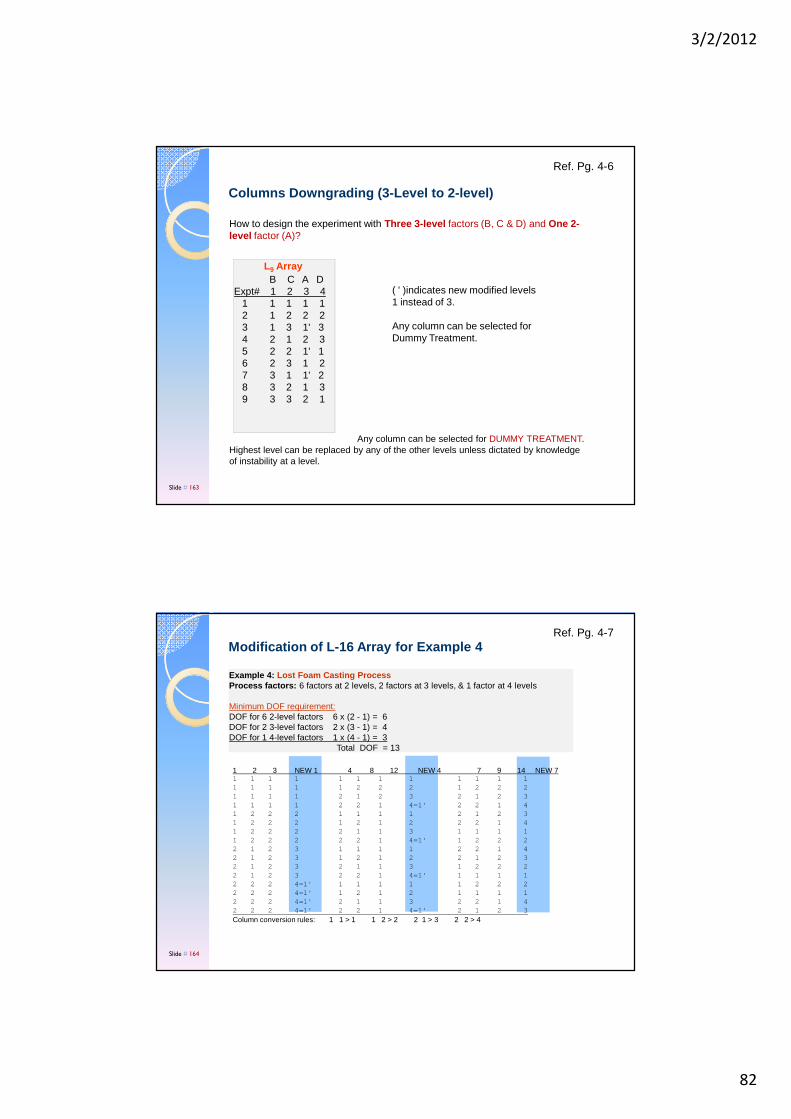
3/2/2012
82
How to design the experiment with Three 3-level factors (B, C & D) and One 2-level factor (A)?
Any column can be selected for DUMMY TREATMENT.Highest level can be replaced by any of the other levels unless dictated by knowledge of instability at a level.
L9 ArrayB C A D
Expt# 1 2 3 41 1 1 1 12 1 2 2 23 1 3 1' 34 2 1 2 35 2 2 1' 16 2 3 1 27 3 1 1' 28 3 2 1 39 3 3 2 1
( ' )indicates new modified levels 1 instead of 3.
Any column can be selected for Dummy Treatment.
Columns Downgrading (3-Level to 2-level)
Ref. Pg. 4-6
Slide # 163
Example 4: Lost Foam Casting ProcessProcess factors: 6 factors at 2 levels, 2 factors at 3 levels, & 1 factor at 4 levels
Minimum DOF requirement:DOF for 6 2-level factors 6 x (2 - 1) = 6DOF for 2 3-level factors 2 x (3 - 1) = 4DOF for 1 4-level factors 1 x (4 - 1) = 3
Total DOF = 13
Modification of L-16 Array for Example 4
1 2 3 NEW 1 4 8 12 NEW 4 7 9 14 NEW 7 1 1 1 1 1 1 1 1 1 1 1 11 1 1 1 1 2 2 2 1 2 2 21 1 1 1 2 1 2 3 2 1 2 31 1 1 1 2 2 1 4=1' 2 2 1 41 2 2 2 1 1 1 1 2 1 2 31 2 2 2 1 2 1 2 2 2 1 41 2 2 2 2 1 1 3 1 1 1 11 2 2 2 2 2 1 4=1' 1 2 2 22 1 2 3 1 1 1 1 2 2 1 42 1 2 3 1 2 1 2 2 1 2 32 1 2 3 2 1 1 3 1 2 2 22 1 2 3 2 2 1 4=1' 1 1 1 12 2 2 4=1' 1 1 1 1 1 2 2 22 2 2 4=1' 1 2 1 2 1 1 1 12 2 2 4=1' 2 1 1 3 2 2 1 42 2 2 4=1' 2 2 1 4=1' 2 1 2 3Column conversion rules: 1 1 > 1 1 2 > 2 2 1 > 3 2 2 > 4
Ref. Pg. 4-7
Slide # 164
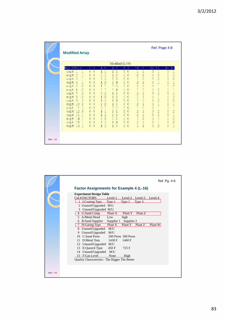
3/2/2012
83
Modified ArrayRef. Page 4-8
Slide # 165
Factor Assignments for Example 4 (L-16)Experiment Design Table Col.# FACTORS Level-1 Level-2 Level-3 Level-4
1 I:Coating Type Type 1 Type 2 Type 3 2 Unused/Upgraded M/U 3 Unused/Upgraded M/U 4 G:Sand Comp Plant X Plant Y Plant Z 5 A:Metal Head Low high 6 B:Sand Supplier Supplier 1 Supplier 2 7 H:Gating Type Plant X Plant Y Plant Z Plant W 8 Unused/Upgraded M/U 9 Unused/Upgraded M/U 10 C:Sand Perm 200 Perm 300 Perm 11 D:Metal Tem. 1430 F 1460 F 12 Unused/Upgraded M/U 13 E:Quench Type 450 F 725 F 14 Unused/Upgraded M/U 15 F:Gas Level None High
Quality Characteristic: The Bigger The Better
Ref. Pg. 4-9
Slide # 166
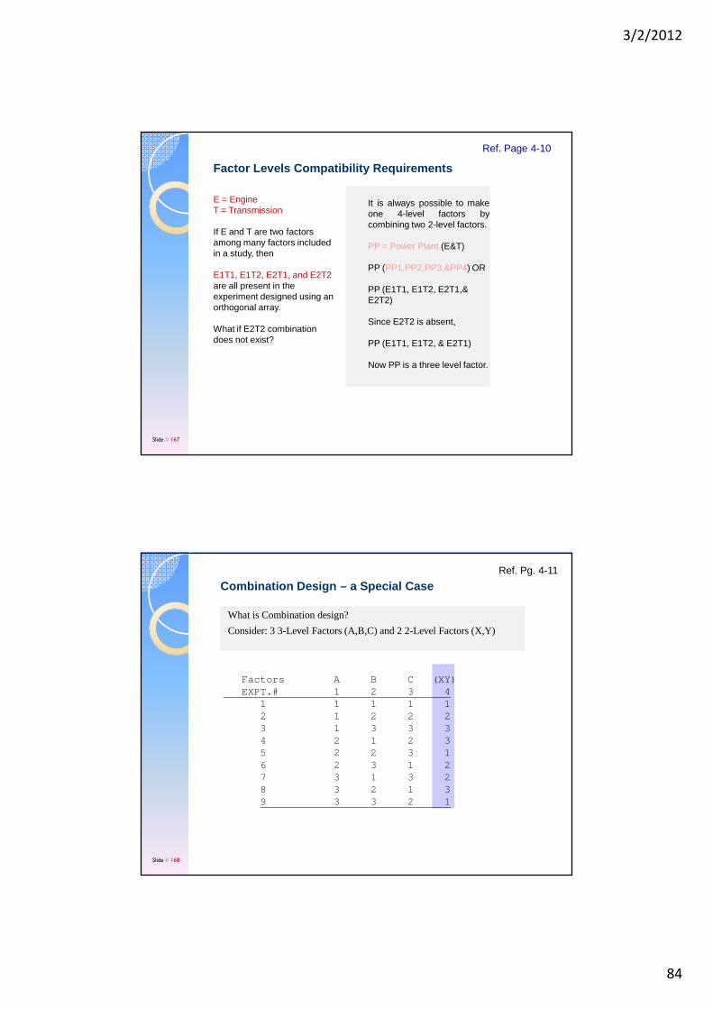
3/2/2012
84
E = EngineT = Transmission
If E and T are two factors among many factors included in a study, then
E1T1, E1T2, E2T1, and E2T2are all present in the experiment designed using an orthogonal array.
What if E2T2 combination does not exist?
Factor Levels Compatibility Requirements
It is always possible to makeone 4-level factors bycombining two 2-level factors.
PP = Power Plant (E&T)
PP (PP1,PP2,PP3,&PP4) OR
PP (E1T1, E1T2, E2T1,& E2T2)
Since E2T2 is absent,
PP (E1T1, E1T2, & E2T1)
Now PP is a three level factor.
Ref. Page 4-10
Slide # 167
What is Combination design?
Consider: 3 3-Level Factors (A,B,C) and 2 2-Level Factors (X,Y)
Combination Design – a Special Case
Factors A B C (XY)EXPT.# 1 2 3 4
1 1 1 1 12 1 2 2 23 1 3 3 34 2 1 2 35 2 2 3 16 2 3 1 27 3 1 3 28 3 2 1 39 3 3 2 1
Ref. Pg. 4-11
Slide # 168
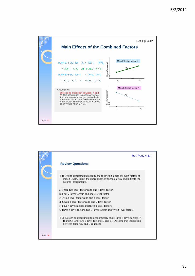
3/2/2012
85
Assumption: There is no interaction between X and Y. This assumption is necessary since the conclusions about the main effects are drawn based on a fixed value of the other factor. The main effect of X above is only valid when Y = Y1.
___ ___MAIN EFFECT OF X = (XY)2 - (XY)1
____ ____= X2Y1 - X1Y1 AT FIXED Y = Y1
___ ___MAIN EFFECT OF Y = (XY)3 - (XY)1
____ ____= X1Y2 - X1Y1 AT FIXED X = X1
Main Effects of the Combined Factors
Res
ult/R
espo
nse/
QC
X1 A3 X2
Res
ult/R
espo
nse/
QC
Y1 A3 Y2
Y1
X1
Main Effect of factor X
Main Effect of factor Y
Ref. Pg. 4-12
Slide # 169
4-1: Design experiments to study the following situations with factors at mixed levels. Select the appropriate orthogonal array and indicate the column assignments.
a. Three two level factors and one 4-level factor
b. Four 2-level factors and one 3-level factor
c. Two 3-level factors and one 2-level factor
d. Seven 3-level factors and one 2-level factor
e. Four 4-level factors and three 2-level factors
f. Three 4-level factors, two 3-level factors and five 2-level factors.
4-2: Design an experiment to economically study three 3-level factors (A, B and C) and two 2-level factors (D and E). Assume that interaction between factors D and E is absent.
Review Questions
Ref. Page 4-13
Slide # 170
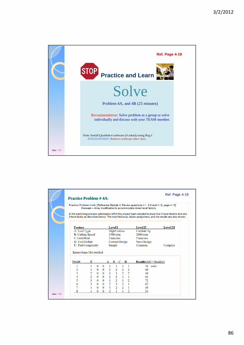
3/2/2012
86
SolveProblem 4A, and 4B (25 minutes)
Recommendation: Solve problem as a group or solve individually and discuss with your TEAM member.
Note: Install Qualitek-4 software (if asked) using Reg.# 409240108100690. Remove software after class.
Ref. Page 4-19
Slide # 171
Practice and Learn
Practice Problem # 4APractice Problem # 4A::Ref. Page 4-19
Slide # 172
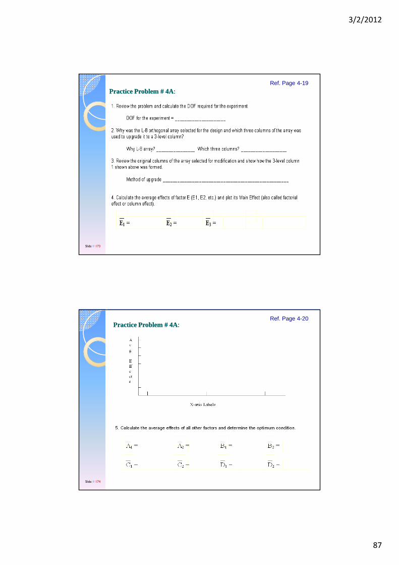
3/2/2012
87
Practice Problem # 4APractice Problem # 4A::Ref. Page 4-19
Slide # 173
Practice Problem # 4APractice Problem # 4A::Ref. Page 4-20
Slide # 174
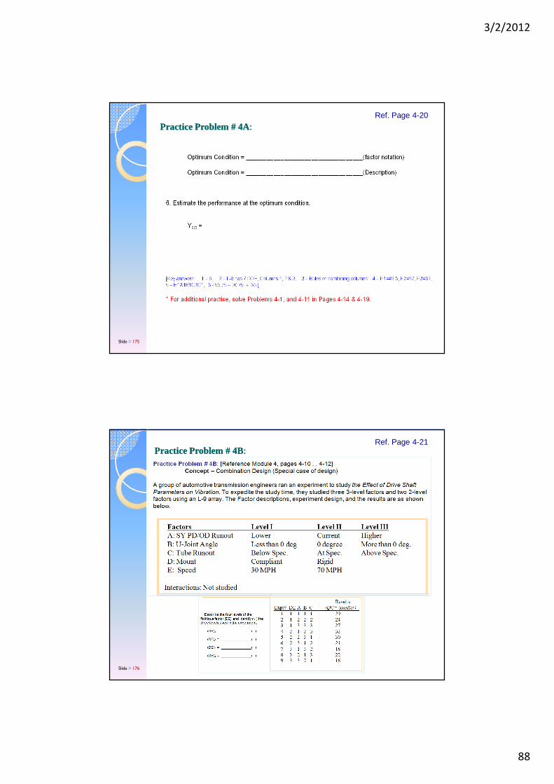
3/2/2012
88
Practice Problem # 4APractice Problem # 4A::Ref. Page 4-20
Slide # 175
Practice Problem # 4BPractice Problem # 4B::Ref. Page 4-21
Slide # 176
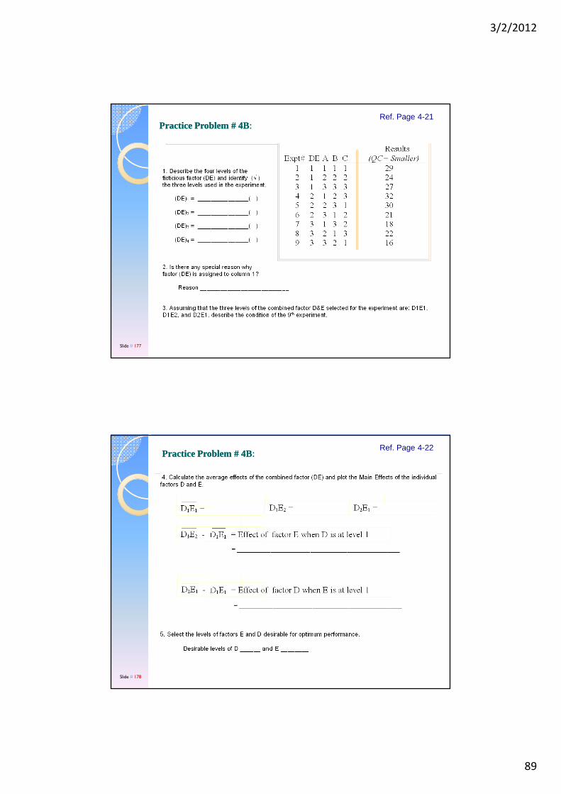
3/2/2012
89
Practice Problem # 4BPractice Problem # 4B::Ref. Page 4-21
Slide # 177
Practice Problem # 4BPractice Problem # 4B::Ref. Page 4-22
Slide # 178

3/2/2012
90
Practice Problem # 4BPractice Problem # 4B::Ref. Page 4-22
Slide # 179
Thoughts for the day . .Thoughts for the day . .
“Give a man a fish and you feed him for a day. Teach a man to fish and you feed him for a lifetime.”
-Chinese Proverb
Slide # 180
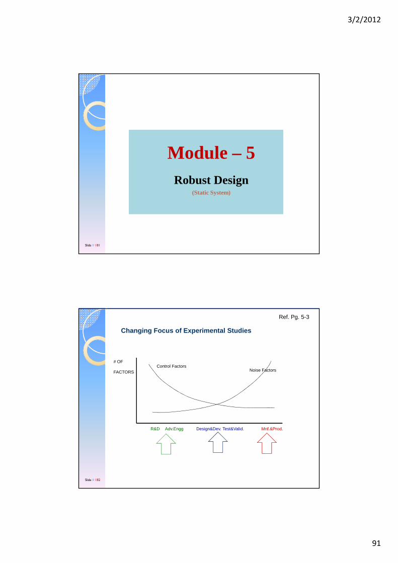
3/2/2012
91
Module – 5Robust Design
(Static System)
Slide # 181
Changing Focus of Experimental Studies
# OF
FACTORS
R&D Adv.Engg Design&Dev. Test&Valid. Mnf.&Prod.
Control FactorsNoise Factors
Ref. Pg. 5-3
Slide # 182
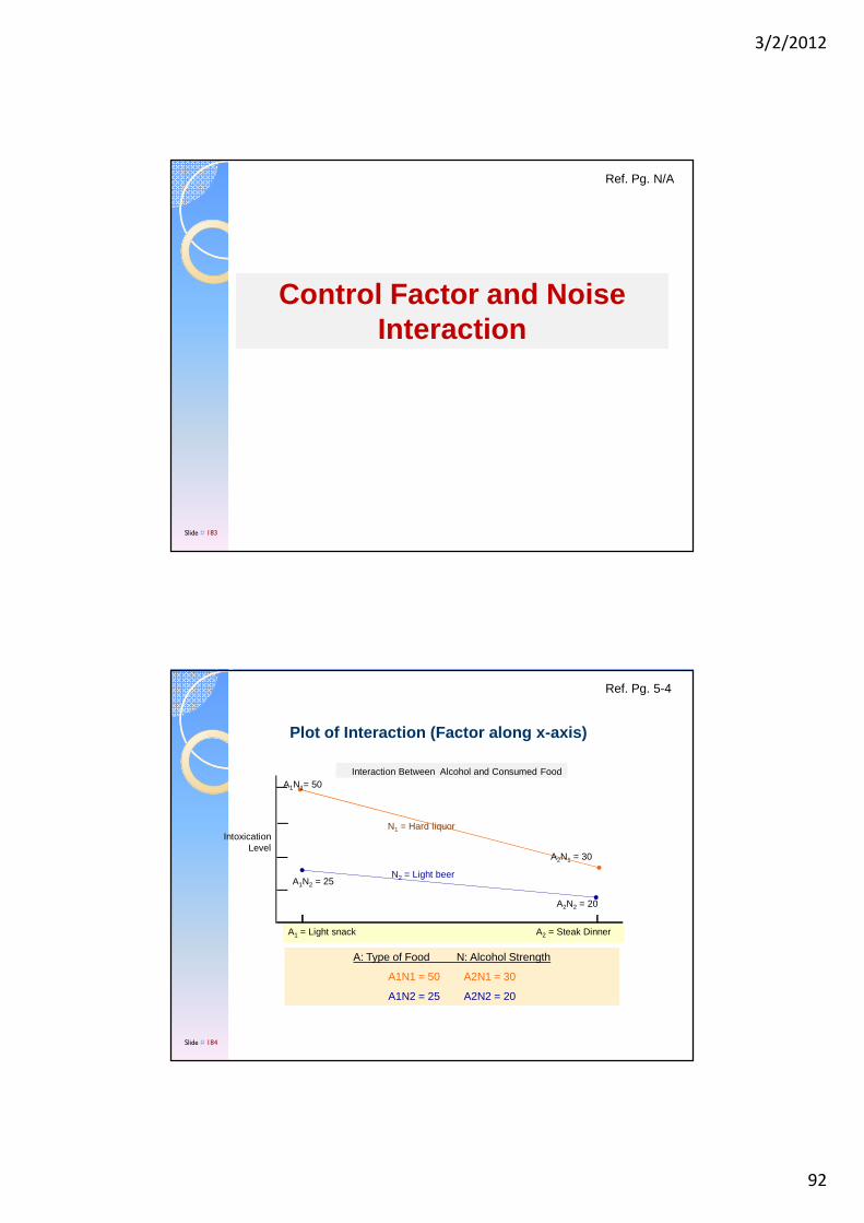
3/2/2012
92
Ref. Pg. N/A
Control Factor and Noise Interaction
Slide # 183
Plot of Interaction (Factor along x-axis)
N1 = Hard liquorIntoxication
Level
A1 = Light snack A2 = Steak Dinner
N2 = Light beerA1N2 = 25
A2N2 = 20
A2N1 = 30
A1N1= 50Interaction Between Alcohol and Consumed Food
A: Type of Food N: Alcohol Strength
A1N1 = 50 A2N1 = 30
A1N2 = 25 A2N2 = 20
Ref. Pg. 5-4
Slide # 184
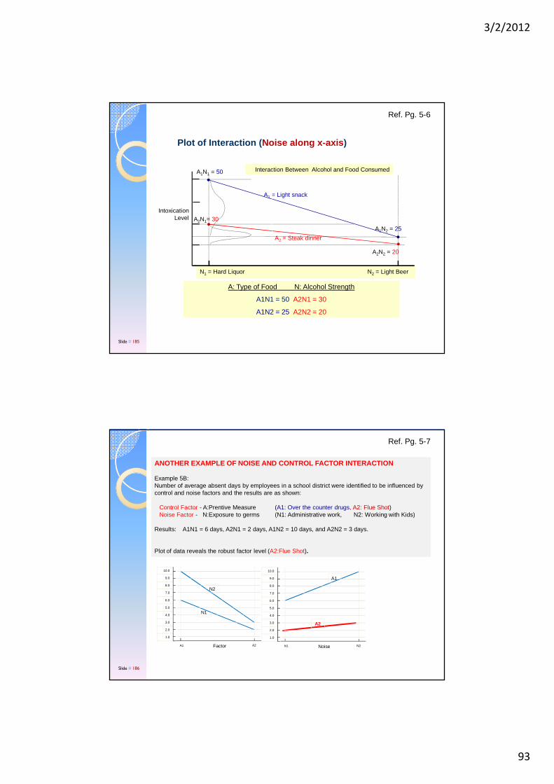
3/2/2012
93
Plot of Interaction ( Noise along x-axis )
A1 = Light snack
A2N2 = 20
A2N1= 30
A2 = Steak dinner
A1N2 = 25
A1N1 = 50 Interaction Between Alcohol and Food Consumed
Intoxication Level
N1 = Hard Liquor N2 = Light Beer
Ref. Pg. 5-6
A: Type of Food N: Alcohol Strength
A1N1 = 50 A2N1 = 30
A1N2 = 25 A2N2 = 20
Slide # 185
8.0
7.0
6.0
5.0
4.0
3.0
2.0
1.0
10.0
9.0
A2A1 Factor
N2
N1
8.0
7.0
6.0
5.0
4.0
3.0
2.0
1.0
10.0
9.0
N2N1 Noise
A2
A1
ANOTHER EXAMPLE OF NOISE AND CONTROL FACTOR INTERAC TION
Example 5B:Number of average absent days by employees in a school district were identified to be influenced by control and noise factors and the results are as shown:
Control Factor - A:Prentive Measure (A1: Over the counter drugs, A2: Flue Shot)Noise Factor - N:Exposure to germs (N1: Administrative work, N2: Working with Kids)
Results: A1N1 = 6 days, A2N1 = 2 days, A1N2 = 10 days, and A2N2 = 3 days.
Plot of data reveals the robust factor level (A2:Flue Shot).
Ref. Pg. 5-7
Slide # 186

3/2/2012
94
We will see how this interaction between noise and control factor is used to determine ROBUST
factor levels soon.
Now, let’s learn about how we can smartly analyze MULTIPLE SAMPLE RESULTS for
DOE.
Ref. Pg. N/A
Slide # 187
11 1 1 1 1 1 1
22 1 1 1 2 2 2
23 1 2 2 1 1 2
14 1 2 2 2 2 1
15 2 1 2 1 2 2
26 2 1 2 2 1 1
27 2 2 1 1 2 1
18 2 2 1 2 1 2
ETr A B - C D F yz z z z z z Sd S/N
12.810 11 9 9 10 11 1.45 -22.2
9.310 12 8 8 10 12 0.85 9.3
12.911.7 11.8 11.5 14.3 14.4 14.1 1.43 12.9
14.112.7 12.7 12.6 15.6 15.6 15.4 1.57 14.1
13.213.8 13.5 13.8 13.3 12.8 12.4 0.56 13.2
14.913.2 13.5 13.4 16.2 16.6 16.4 1.67 14.9
13.912.6 12.9 12.1 15.4 15.8 14.8 1.59 13.9
13.312.3 11.7 12 15.1 14.3 14.2 1.43 13.3
Results (y)__
Grand Averages => 13.1 1.32 13.1
Average
-
10
10
Multiple Sample Results of Planned Experiments
Is the result of trial#1 better than that of trial#2?It is difficult to objectively answer using AVERAGE of results only.
Ref. Pg. N/A
Slide # 188
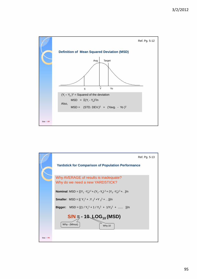
3/2/2012
95
Definition of Mean Squared Deviation (MSD)
Avg. Target
_yi Y Yo
Ref. Pg. 5-12
(Yi – Yo )2 = Squared of the deviation
MSD = Σ(Yi - Yo)2/nAlso,
MSD = (STD. DEV.)2 + (Yavg. - Yo )2
Slide # 189
Why AVERAGE of results is inadequate?Why do we need a new YARDSTICK?
Nominal : MSD = [(Y1 -Yo) 2 +.(Y2 -Yo) 2 + (Y3 -Yo) 2 +. .]/n
Smaller : MSD = [( Y12 + .Y 2
2 +Y 32 + . .)]/n
Bigger: MSD = [(1 / Y12 + 1 / Y2
2 + 1/Y32 + ...... )]/n
S/N = - 10 LOG10 (MSD)Why - (Minus) Why 10
Yardstick for Comparison of Population Performance
Ref. Pg. 5-13
Slide # 190

3/2/2012
96
Logarithmic Measure of Sound Volume(Common household audio surround sound system)
Lower Volume => Lower Volume => Lower Volume => Lower Volume => Lower Volume => Lower Volume => Lower Volume => Lower Volume => -------- 60 dB Higher volume=> 60 dB Higher volume=> 60 dB Higher volume=> 60 dB Higher volume=> 60 dB Higher volume=> 60 dB Higher volume=> 60 dB Higher volume=> 60 dB Higher volume=> -------- 12 dB 12 dB 12 dB 12 dB 12 dB 12 dB 12 dB 12 dB (Range of Scale 0 to (Range of Scale 0 to (Range of Scale 0 to (Range of Scale 0 to (Range of Scale 0 to (Range of Scale 0 to (Range of Scale 0 to (Range of Scale 0 to –––––––– 100 dB)100 dB)100 dB)100 dB)100 dB)100 dB)100 dB)100 dB)
Note: Lower magnitude of negative number is HIGHER as in S/N RatioNote: Lower magnitude of negative number is HIGHER as in S/N RatioNote: Lower magnitude of negative number is HIGHER as in S/N RatioNote: Lower magnitude of negative number is HIGHER as in S/N RatioNote: Lower magnitude of negative number is HIGHER as in S/N RatioNote: Lower magnitude of negative number is HIGHER as in S/N RatioNote: Lower magnitude of negative number is HIGHER as in S/N RatioNote: Lower magnitude of negative number is HIGHER as in S/N Ratio
Ref. Pg. N/A
191Slide # 191
The magnitude of most earthquakes is measured on the Richter scale, invented by Charles F. Richter in 1934. The Richter magnitude is calculated from the amplitude of the largest seismic wave recorded for the earthquake, no matter what type of wave was the strongest.
The Richter magnitudes are based on a logarithmic scale (base 10). What this means is that for each whole number you go up on the Richter scale, the amplitude of the ground motion recorded by a seismograph goes up ten times.Using this scale, a magnitude 5 earthquake would result in ten times the level of ground shaking as a magnitude 4 earthquake (and 32 times as much energy would be released). To give you an idea how these numbers can add up, think of it in terms of the energy released by explosives: a magnitude 1 seismic wave releases as much energy as blowing up 6 ounces of TNT. A magnitude 8 earthquake releases as much energy as detonating 6 million tons of TNT. Pretty impressive, huh? Fortunately, most of the earthquakes that occur each year are magnitude 2.5 or less, too small to be felt by most people.
Body-wave magnitude formula:
mb = log(A/T) + Q(D,h)
where A is the ground motion (in microns)T is the wave's period (in seconds), and Q(D,h) is a correction factor that depends on distance
to the quake's epicenter D (in degrees) and focal depth h (in kilometers).
Ref. Pg. N/A
Slide # 192
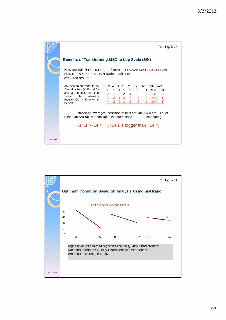
3/2/2012
97
How are S/N Ratios compared? (QUALITEK-4 software output, SEM-EX06.Q4W)
How can we transform S/N Ratios back into expected results?
Based on averages, condition results of trials 3 & 4 are equal.Based on S/N ratios, condition 3 is better, since comparing
-14.1 > -14.4 ( -14.1 is bigger than -14.4)
EXPT. A B C R1 R2 R3 S/N AVG.1 1 1 1 2 3 4 -9.86 32 1 2 2 4 5 3 -12.2 43 2 1 2 4 5 6 -14.1 54 2 2 1 3 5 7 -14.4 5
An experiment with three2-level factors (A, B and C)and 3 samples per trialyielded the followingresults (QC = Smaller isBetter)
Benefits of Transforming MSD to Log Scale (S/N)
Ref. Pg. 5-14
Slide # 193
Highest values selected regardless of the Quality Characteristic.Does that mean the Quality Characteristic has no effect?When does it come into play?
A1 A2 B1 B2 C1 C2
T
-15
-14
-13
-11
-12
Plot of Factor Average Effects
Optimum Condition Based on Analysis Using S/N Ratio
Ref. Pg. 5-14
Slide # 194
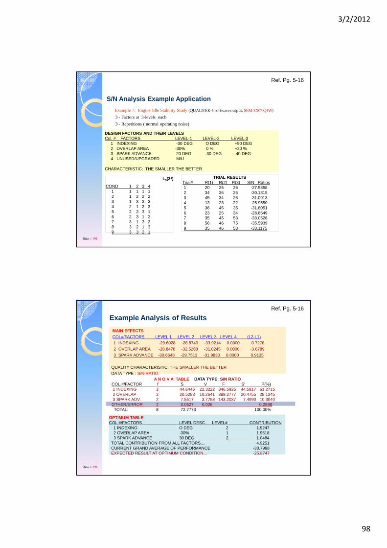
3/2/2012
98
Example 7: Engine Idle Stability Study(QUALITEK-4 software output, SEM-EX07.Q4W)
3 - Factors at 3-levels each
3 - Repetitions ( normal operating noise)
DESIGN FACTORS AND THEIR LEVELSCol. # FACTORS LEVEL-1 LEVEL-2 LEVEL-3
1 INDEXING -30 DEG O DEG +50 DEG2 OVERLAP AREA -30% 0 % +30 %3 SPARK ADVANCE 20 DEG 30 DEG 40 DEG4 UNUSED/UPGRADED M/U
CHARACTERISTIC: THE SMALLER THE BETTER
L9(34)
COND 1 2 3 41 1 1 1 12 1 2 2 23 1 3 3 34 2 1 2 35 2 2 3 1 6 2 3 1 27 3 1 3 28 3 2 1 39 3 3 2 1
TRIAL RESULTS Trial# R(1) R(2) R(3) S/N Ratios 1 20 25 26 -27.5358 2 34 36 26 -30.1815 3 45 34 26 -31.0913 4 13 23 22 -25.9550 5 36 45 35 -31.8051 6 23 25 34 -28.86497 35 45 53 -33.0528 8 56 46 75 -35.5939 9 35 46 53 -33.1175
S/N Analysis Example Application
Ref. Pg. 5-16
Slide # 195
Example Analysis of Results
MAIN EFFECTSCOL#/FACTORS LEVEL 1 LEVEL 2 LEVEL 3 LEVEL 4 (L2-L1)1 INDEXING -29.6028 -28.8749 -33.9214 0.0000 0.72782 OVERLAP AREA -28.8478 -32.5268 -31.0245 0.0000 -3.67893 SPARK ADVANCE -30.6648 -29.7513 -31.9830 0.0000 0.9135
QUALITY CHARACTERISTIC: THE SMALLER THE BETTERDATA TYPE : S/N RATIO
OPTIMUM TABLECOL #/FACTORS LEVEL DESC. LEVEL# CONTRIBUTION
1 INDEXING O DEG 2 1.92472 OVERLAP AREA -30% 1 1.95183 SPARK ADVANCE 30 DEG 2 1.0484
TOTAL CONTRIBUTION FROM ALL FACTORS.... 4.9251CURRENT GRAND AVERAGE OF PERFORMANCE -30.7998EXPECTED RESULT AT OPTIMUM CONDITION... -25.8747
A N O V A TABLE DATA TYPE: S/N RATIO COL.#/FACTOR f S V F S' P(%)1 INDEXING 2 44.6445 22.3222 846.5925 44.5917 61.27152 OVERLAP 2 20.5283 10.2641 389.2777 20.4755 28.13453 SPARK ADV. 2 7.5517 3.7758 143.2037 7.4990 10.3040OTHER/ERROR 2 0.0527 0.026 0.2898TOTAL: 8 72.7773 100.00%
Ref. Pg. 5-16
Slide # 196

3/2/2012
99
Multiple Factor Levels for Robustness against single noise
Ref. Pg. N/A
Slide # 197
Steps for Robust Design with Multiple Factors
Ref. Pg. N/A
Slide # 198
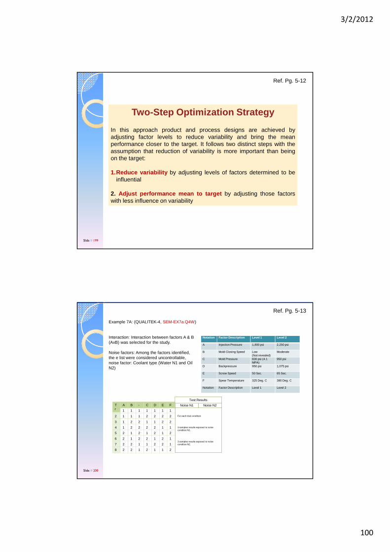
3/2/2012
100
Two-Step Optimization Strategy
In this approach product and process designs are achieved byadjusting factor levels to reduce variability and bring the meanperformance closer to the target. It follows two distinct steps with theassumption that reduction of variability is more important than beingon the target:
1.Reduce variability by adjusting levels of factors determined to beinfluential
2. Adjust performance mean to target by adjusting those factorswith less influence on variability
Ref. Pg. 5-12
Slide # 199
11 1 1 1 1 1 1
22 1 1 1 2 2 2
23 1 2 2 1 1 2
14 1 2 2 2 2 1
15 2 1 2 1 2 2
26 2 1 2 2 1 1
27 2 2 1 1 2 1
18 2 2 1 2 1 2
ETr
A B - C D F Noise N1 Noise N2
Test Results
For each trial condition:
3 samples results exposed to noise condition N1.
3 samples results exposed to noise condition N2.
Notation Factor Description Level 1 Level 2
A Injection Pressure 1,800 psi 2,250 psi
B Mold Closing Speed Low(Not revealed)
Moderate
C Mold Pressure 600 psi (4.1 MPA)
950 psi
D Backpressure 950 psi 1,075 psi
E Screw Speed 50 Sec. 65 Sec.
F Spear Temperature 325 Deg. C 380 Deg. C
Notation Factor Description Level 1 Level 2
Example 7A: (QUALITEK-4, SEM-EX7a.Q4W)
Interaction: Interaction between factors A & B (AxB) was selected for the study.
Noise factors: Among the factors identified, the e list were considered uncontrollable, noise factor: Coolant type (Water N1 and Oil N2)
Ref. Pg. 5-13
Slide # 200
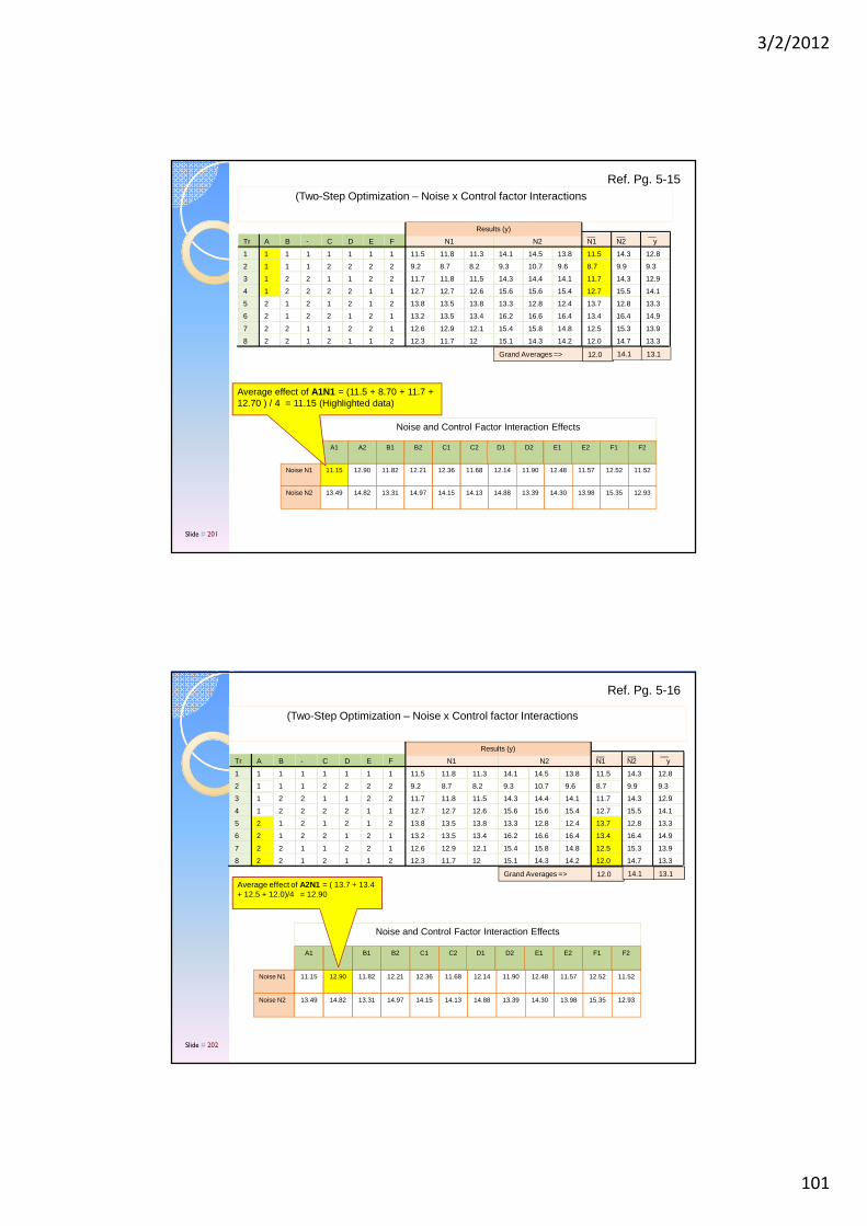
3/2/2012
101
11 1 1 1 1 1 1
22 1 1 1 2 2 2
23 1 2 2 1 1 2
14 1 2 2 2 2 1
15 2 1 2 1 2 2
26 2 1 2 2 1 1
27 2 2 1 1 2 1
18 2 2 1 2 1 2
ETr A B - C D F N1z z z z z z N2 y
11.511.5 11.8 11.3 14.1 14.5 13.8 14.3 12.8
8.79.2 8.7 8.2 9.3 10.7 9.6 9.9 9.3
11.711.7 11.8 11.5 14.3 14.4 14.1 14.3 12.9
12.712.7 12.7 12.6 15.6 15.6 15.4 15.5 14.1
13.713.8 13.5 13.8 13.3 12.8 12.4 12.8 13.3
13.413.2 13.5 13.4 16.2 16.6 16.4 16.4 14.9
12.512.6 12.9 12.1 15.4 15.8 14.8 15.3 13.9
12.012.3 11.7 12 15.1 14.3 14.2 14.7 13.3
N1 N2
Results (y)______
Grand Averages => 12.0 14.1 13.1
(Two-Step Optimization – Noise x Control factor Interactions
Noise and Control Factor Interaction Effects
Noise N1
Noise N2
11.15 12.90 11.82 12.21 12.36 11.68 12.14 11.90 12.48 11.57 12.52 11.52
13.49 14.82 13.31 14.97 14.15 14.13 14.88 13.39 14.30 13.98 15.35 12.93
A1 A2 B1 B2 C1 C2 D1 D2 E1 E2 F1 F2
Average effect of A1N1 = (11.5 + 8.70 + 11.7 + 12.70 ) / 4 = 11.15 (Highlighted data)
Ref. Pg. 5-15
Slide # 201
11 1 1 1 1 1 1
22 1 1 1 2 2 2
23 1 2 2 1 1 2
14 1 2 2 2 2 1
15 2 1 2 1 2 2
26 2 1 2 2 1 1
27 2 2 1 1 2 1
18 2 2 1 2 1 2
ETr A B - C D F N1z z z z z z N2 y
11.511.5 11.8 11.3 14.1 14.5 13.8 14.3 12.8
8.79.2 8.7 8.2 9.3 10.7 9.6 9.9 9.3
11.711.7 11.8 11.5 14.3 14.4 14.1 14.3 12.9
12.712.7 12.7 12.6 15.6 15.6 15.4 15.5 14.1
13.713.8 13.5 13.8 13.3 12.8 12.4 12.8 13.3
13.413.2 13.5 13.4 16.2 16.6 16.4 16.4 14.9
12.512.6 12.9 12.1 15.4 15.8 14.8 15.3 13.9
12.012.3 11.7 12 15.1 14.3 14.2 14.7 13.3
N1 N2
Results (y)______
Grand Averages => 12.0 14.1 13.1
(Two-Step Optimization – Noise x Control factor Interactions
Noise and Control Factor Interaction Effects
Noise N1
Noise N2
11.15 12.90 11.82 12.21 12.36 11.68 12.14 11.90 12.48 11.57 12.52 11.52
13.49 14.82 13.31 14.97 14.15 14.13 14.88 13.39 14.30 13.98 15.35 12.93
A1 A2 B1 B2 C1 C2 D1 D2 E1 E2 F1 F2
Average effect of A2N1 = ( 13.7 + 13.4 + 12.5 + 12.0)/4 = 12.90
Ref. Pg. 5-16
Slide # 202
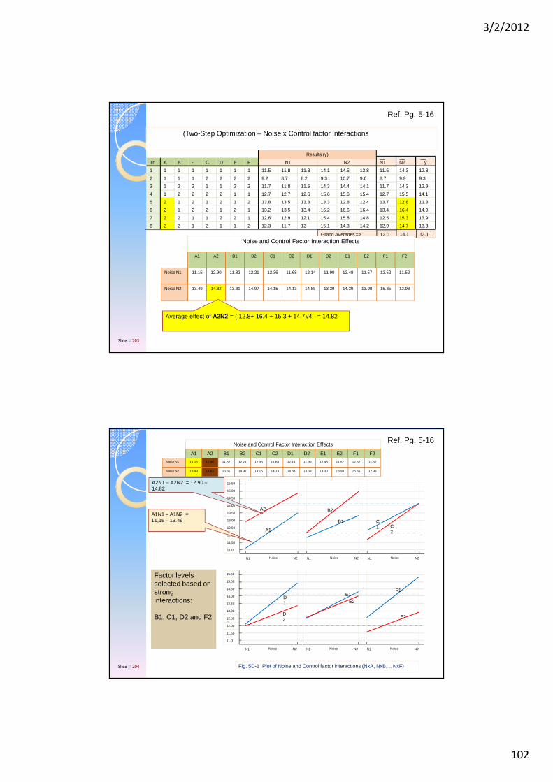
3/2/2012
102
11 1 1 1 1 1 1
22 1 1 1 2 2 2
23 1 2 2 1 1 2
14 1 2 2 2 2 1
15 2 1 2 1 2 2
26 2 1 2 2 1 1
27 2 2 1 1 2 1
18 2 2 1 2 1 2
ETr A B - C D F N1z z z z z z N2 y
11.511.5 11.8 11.3 14.1 14.5 13.8 14.3 12.8
8.79.2 8.7 8.2 9.3 10.7 9.6 9.9 9.3
11.711.7 11.8 11.5 14.3 14.4 14.1 14.3 12.9
12.712.7 12.7 12.6 15.6 15.6 15.4 15.5 14.1
13.713.8 13.5 13.8 13.3 12.8 12.4 12.8 13.3
13.413.2 13.5 13.4 16.2 16.6 16.4 16.4 14.9
12.512.6 12.9 12.1 15.4 15.8 14.8 15.3 13.9
12.012.3 11.7 12 15.1 14.3 14.2 14.7 13.3
N1 N2
Results (y)______
Grand Averages => 12.0 14.1 13.1
(Two-Step Optimization – Noise x Control factor Interactions
Noise and Control Factor Interaction Effects
Noise N1
Noise N2
11.15 12.90 11.82 12.21 12.36 11.68 12.14 11.90 12.48 11.57 12.52 11.52
13.49 14.82 13.31 14.97 14.15 14.13 14.88 13.39 14.30 13.98 15.35 12.93
A1 A2 B1 B2 C1 C2 D1 D2 E1 E2 F1 F2
Average effect of A2N2 = ( 12.8+ 16.4 + 15.3 + 14.7)/4 = 14.82
Ref. Pg. 5-16
Slide # 203
Noise and Control Factor Interaction Effects
Noise N1
Noise N2
11.15 12.90 11.82 12.21 12.36 11.68 12.14 11.90 12.48 11.57 12.52 11.52
13.49 14.82 13.31 14.97 14.15 14.13 14.88 13.39 14.30 13.98 15.35 12.93
A1 A2 B1 B2 C1 C2 D1 D2 E1 E2 F1 F2
14.50
14.00
13.50
13.00
12.50xx12.00
11.50
11.0
15.50
15.00
N2N1 Noise N2N1 Noise N2N1 Noise
B1
A1
C1
A2 B2
C2
14.50
14.00
13.50
13.00
12.50xx12.00
11.50
11.0
15.50
15.00
N2N1 Noise N2N1 Noise N2N1 Noise
D1
E1F1
D2
E2
F2
Fig. 5D-1 Plot of Noise and Control factor interactions (NxA, NxB, .. NxF)
A2N1 – A2N2 = 12.90 –14.82
A1N1 – A1N2 = 11,15 – 13.49
Factor levels selected based on strong interactions:
B1, C1, D2 and F2
Ref. Pg. 5-16
Slide # 204
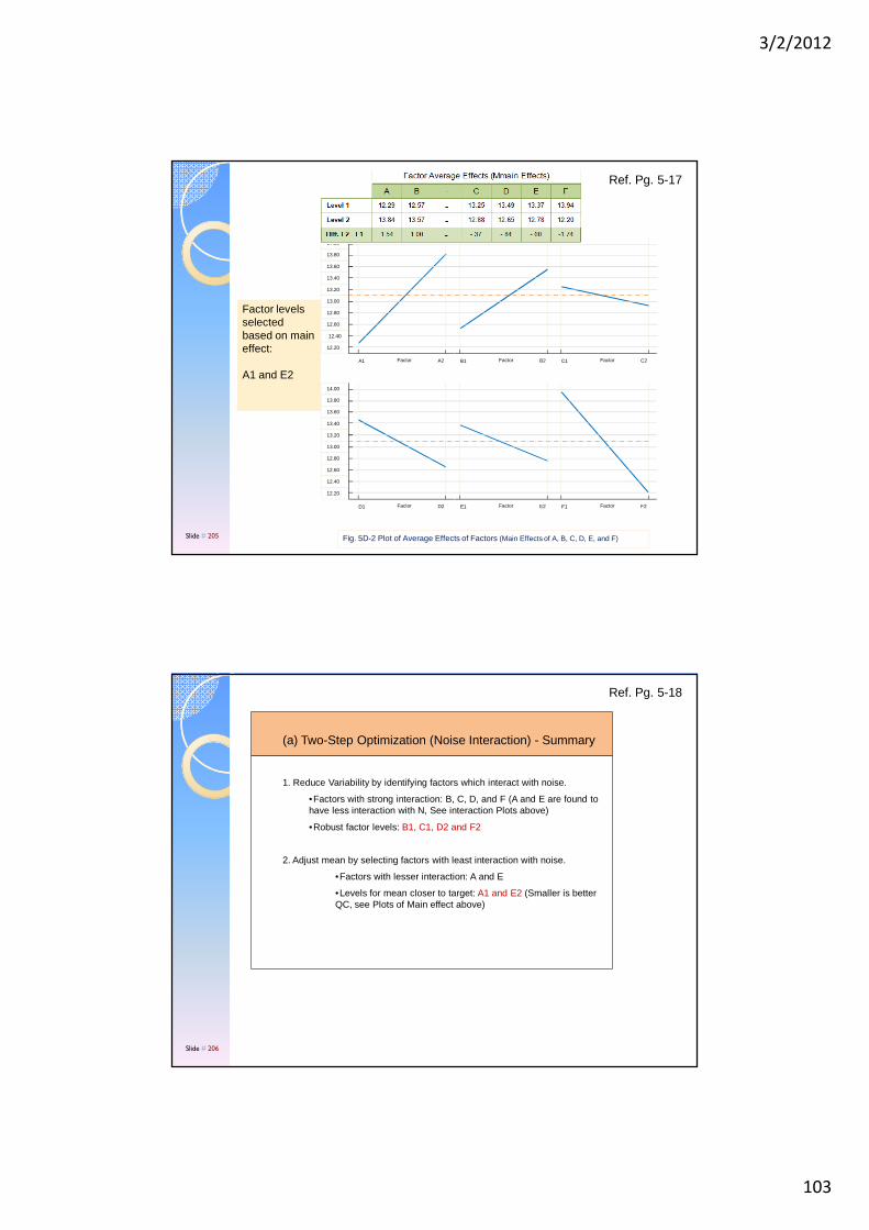
3/2/2012
103
13.60
13.40
13.20
13.00
12.80
12.60
12.40
12.20
14.00
13.80
A2A1 Factor B2B1 Factor C2C1 Factor
13.60
13.40
13.20
13.00
12.80
12.60
12.40
12.20
14.00
13.80
D2D1 Factor E2E1 Factor F2F1 Factor
Fig. 5D-2 Plot of Average Effects of Factors (Main Effects of A, B, C, D, E, and F)
Factor levels selected based on main effect:
A1 and E2
Ref. Pg. 5-17
Slide # 205
(a) Two-Step Optimization (Noise Interaction) - Summary
1. Reduce Variability by identifying factors which interact with noise.
•Factors with strong interaction: B, C, D, and F (A and E are found to have less interaction with N, See interaction Plots above)
•Robust factor levels: B1, C1, D2 and F2
2. Adjust mean by selecting factors with least interaction with noise.
•Factors with lesser interaction: A and E
•Levels for mean closer to target: A1 and E2 (Smaller is better QC, see Plots of Main effect above)
Ref. Pg. 5-18
Slide # 206
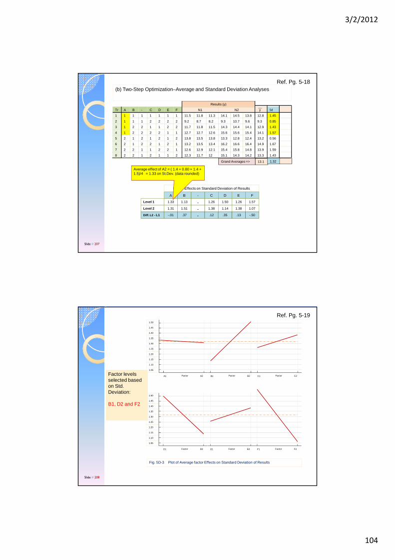
3/2/2012
104
11 1 1 1 1 1 1
22 1 1 1 2 2 2
23 1 2 2 1 1 2
14 1 2 2 2 2 1
15 2 1 2 1 2 2
26 2 1 2 2 1 1
27 2 2 1 1 2 1
18 2 2 1 2 1 2
ETr A B - C D F yz z z z z z Sd
12.811.5 11.8 11.3 14.1 14.5 13.8 1.45
9.39.2 8.7 8.2 9.3 10.7 9.6 0.85
12.911.7 11.8 11.5 14.3 14.4 14.1 1.43
14.112.7 12.7 12.6 15.6 15.6 15.4 1.57
13.213.8 13.5 13.8 13.3 12.8 12.4 0.56
14.913.2 13.5 13.4 16.2 16.6 16.4 1.67
13.912.6 12.9 12.1 15.4 15.8 14.8 1.59
13.312.3 11.7 12 15.1 14.3 14.2 1.43
N1 N2
Results (y)__
Grand Averages => 13.1 1.32
(b) Two-Step Optimization–Average and Standard Deviation Analyses
Factor Effects on Standard Deviation of Results
A B - C D E F
1.33 1.13 - 1.26 1.50 1.26 1.57Level 1
1.31 1.51 - 1.38 1.14 1.38 1.07Level 2
-.01 .37 - .12 .35 .13 -.50Diff. L2 - L1
Average effect of A2 = ( 1.4 + 0.80 + 1.4 + 1.5)/4 = 1.33 on St.Dev. (data rounded)
Ref. Pg. 5-18
Slide # 207
1.40
1.35
1.30
1.25
1.20
1.15
1.10
1.05
1.50
1.45
A2A1 Factor B2B1 Factor C2C1 Factor
1.40
1.35
1.30
1.25
1.20
1.15
1.10
1.05
1.50
1.45
D2D1 Factor E2E1 Factor F2F1 Factor
Fig. 5D-3 Plot of Average factor Effects on Standard Deviation of Results
Factor levels selected based on Std. Deviation:
B1, D2 and F2
Ref. Pg. 5-19
Slide # 208
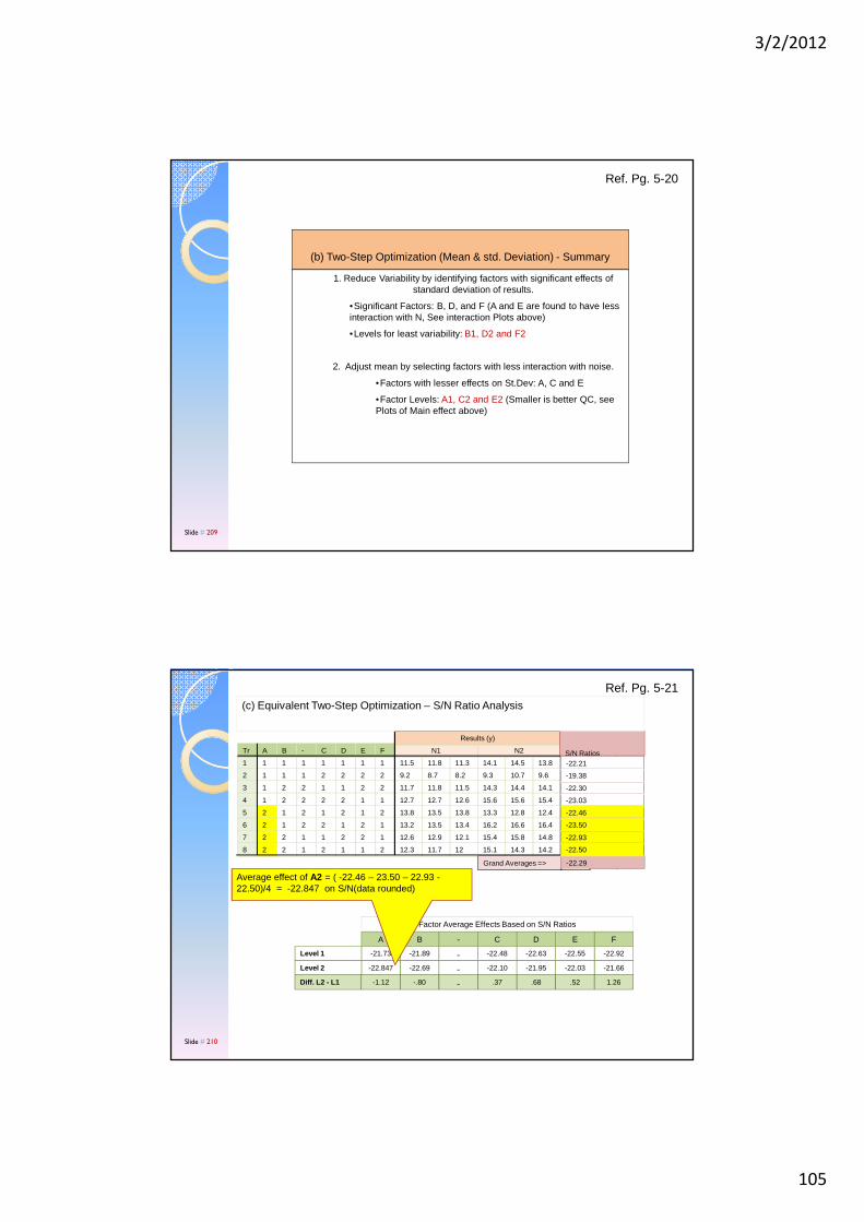
3/2/2012
105
(b) Two-Step Optimization (Mean & std. Deviation) - Summary
1. Reduce Variability by identifying factors with significant effects of standard deviation of results.
•Significant Factors: B, D, and F (A and E are found to have less interaction with N, See interaction Plots above)
•Levels for least variability: B1, D2 and F2
2. Adjust mean by selecting factors with less interaction with noise.
•Factors with lesser effects on St.Dev: A, C and E
•Factor Levels: A1, C2 and E2 (Smaller is better QC, see Plots of Main effect above)
Ref. Pg. 5-20
Slide # 209
11 1 1 1 1 1 1
22 1 1 1 2 2 2
23 1 2 2 1 1 2
14 1 2 2 2 2 1
15 2 1 2 1 2 2
26 2 1 2 2 1 1
27 2 2 1 1 2 1
18 2 2 1 2 1 2
ETr A B - C D F yz z z z z z Sd S/N
12.811.5 11.8 11.3 14.1 14.5 13.8 1.45 -22.2
9.39.2 8.7 8.2 9.3 10.7 9.6 0.85 9.3
12.911.7 11.8 11.5 14.3 14.4 14.1 1.43 12.9
14.112.7 12.7 12.6 15.6 15.6 15.4 1.57 14.1
13.213.8 13.5 13.8 13.3 12.8 12.4 0.56 13.2
14.913.2 13.5 13.4 16.2 16.6 16.4 1.67 14.9
13.912.6 12.9 12.1 15.4 15.8 14.8 1.59 13.9
13.312.3 11.7 12 15.1 14.3 14.2 1.43 13.3
N1 N2
Results (y)__
Grand Averages => 13.1 1.32 13.1
S/N Ratios
-22.29
-22.30
-23.03
-22.21
-19.38
-22.93
-22.50
-22.46
-23.50
(c) Equivalent Two-Step Optimization – S/N Ratio Analysis
Factor Average Effects Based on S/N Ratios
A B - C D E F
-21.73 -21.89 - -22.48 -22.63 -22.55 -22.92Level 1
-22.847 -22.69 - -22.10 -21.95 -22.03 -21.66Level 2
-1.12 -.80 - .37 .68 .52 1.26Diff. L2 - L1
Average effect of A2 = ( -22.46 – 23.50 – 22.93 -22.50)/4 = -22.847 on S/N(data rounded)
Ref. Pg. 5-21
Slide # 210
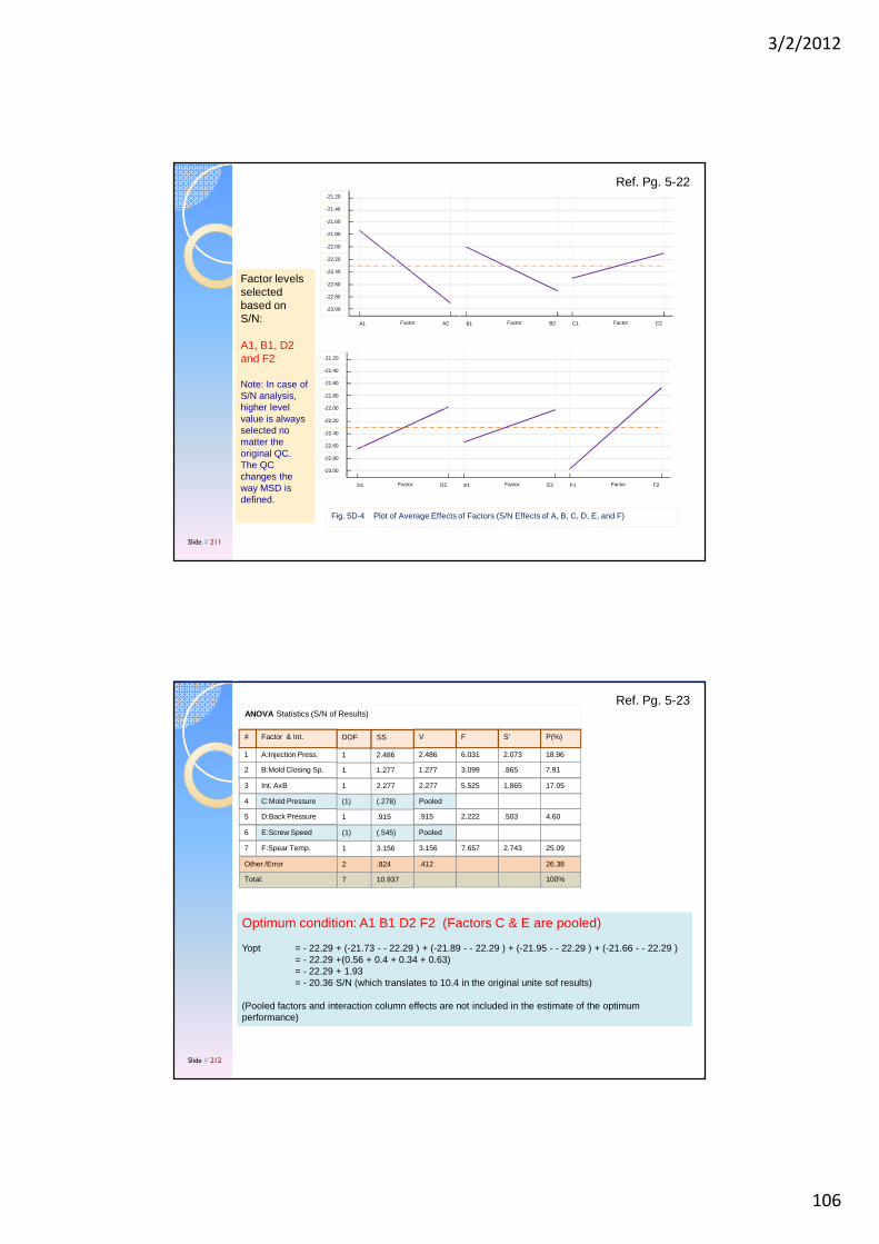
3/2/2012
106
-21.60
-21.80
-22.00
-22.20
-22.40
-22.60
-22.80
-23.00
-21.20
-21.40
A2A1 Factor B2B1 Factor C2C1 Factor
-21.60
-21.80
-22.00
-22.20
-22.40
-22.60
-22.80
-23.00
-21.20
-21.40
D2D1 Factor E2E1 Factor F2F1 Factor
Fig. 5D-4 Plot of Average Effects of Factors (S/N Effects of A, B, C, D, E, and F)
Factor levels selected based on S/N:
A1, B1, D2 and F2
Note: In case of S/N analysis, higher level value is always selected no matter the original QC. The QC changes the way MSD is defined.
Ref. Pg. 5-22
Slide # 211
1 1A:Injection Press. 2.073 18.966.0312.4862.486
2Other /Error 26.38.412.824
7Total: 100%10.937
2 1B:Mold Closing Sp. .865 7.913.0991.2771.277
3 1Int. AxB 1.865 17.055.5252.2772.277
4 (1)C:Mold Pressure Pooled(.278)
5 1D:Back Pressure .503 4.602.222.915.915
6 (1)E:Screw Speed Pooled(.545)
7 1F:Spear Temp. 2.743 25.097.6573.1563.156
ANOVA Statistics (S/N of Results)
# DOFFactor & Int. S’ P(%)FVSS
Optimum condition: A1 B1 D2 F2 (Factors C & E are pooled)
Yopt = - 22.29 + (-21.73 - - 22.29 ) + (-21.89 - - 22.29 ) + (-21.95 - - 22.29 ) + (-21.66 - - 22.29 )= - 22.29 +(0.56 + 0.4 + 0.34 + 0.63)= - 22.29 + 1.93= - 20.36 S/N (which translates to 10.4 in the original unite sof results)
(Pooled factors and interaction column effects are not included in the estimate of the optimum performance)
Ref. Pg. 5-23
Slide # 212
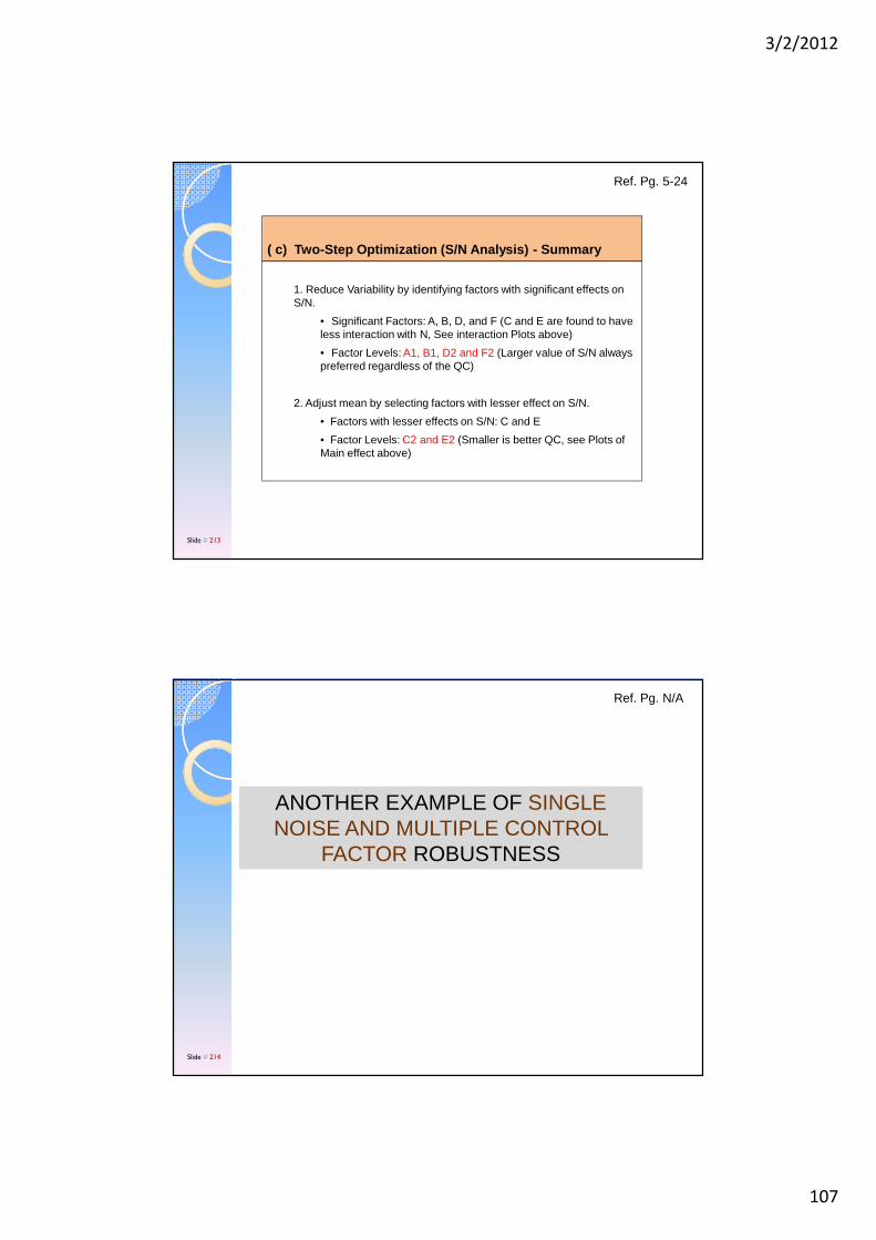
3/2/2012
107
( c) Two-Step Optimization (S/N Analysis) - Summary
1. Reduce Variability by identifying factors with significant effects on S/N.
• Significant Factors: A, B, D, and F (C and E are found to have less interaction with N, See interaction Plots above)
• Factor Levels: A1, B1, D2 and F2 (Larger value of S/N always preferred regardless of the QC)
2. Adjust mean by selecting factors with lesser effect on S/N.
• Factors with lesser effects on S/N: C and E
• Factor Levels: C2 and E2 (Smaller is better QC, see Plots of Main effect above)
Ref. Pg. 5-24
Slide # 213
ANOTHER EXAMPLE OF SINGLE NOISE AND MULTIPLE CONTROL
FACTOR ROBUSTNESS
Ref. Pg. N/A
Slide # 214
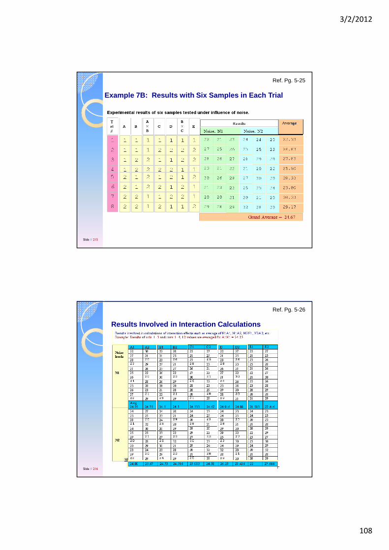
3/2/2012
108
Example 7B: Results with Six Samples in Each Trial
Ref. Pg. 5-25
Slide # 215
Results Involved in Interaction Calculations
Ref. Pg. 5-26
Slide # 216
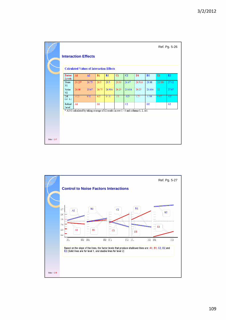
3/2/2012
109
Interaction Effects
Ref. Pg. 5-26
Slide # 217
Control to Noise Factors Interactions
Ref. Pg. 5-27
Slide # 218
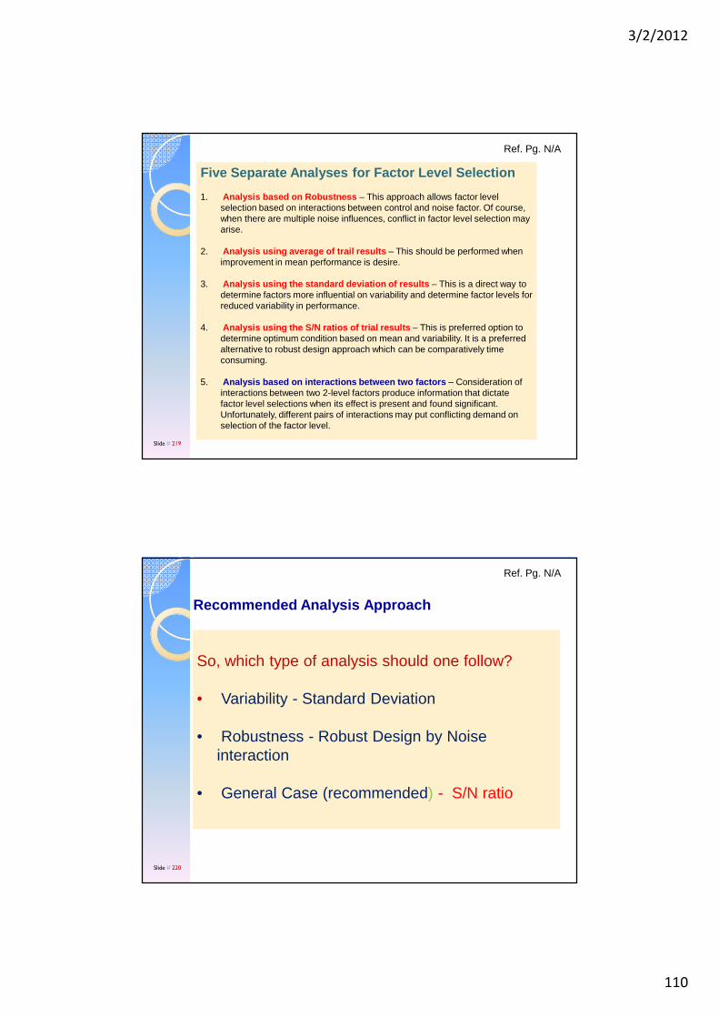
3/2/2012
110
Five Separate Analyses for Factor Level Selection
1. Analysis based on Robustness – This approach allows factor level selection based on interactions between control and noise factor. Of course, when there are multiple noise influences, conflict in factor level selection may arise.
2. Analysis using average of trail results – This should be performed when improvement in mean performance is desire.
3. Analysis using the standard deviation of results – This is a direct way to determine factors more influential on variability and determine factor levels for reduced variability in performance.
4. Analysis using the S/N ratios of trial results – This is preferred option to determine optimum condition based on mean and variability. It is a preferred alternative to robust design approach which can be comparatively time consuming.
5. Analysis based on interactions between two factors – Consideration of interactions between two 2-level factors produce information that dictate factor level selections when its effect is present and found significant. Unfortunately, different pairs of interactions may put conflicting demand on selection of the factor level.
Ref. Pg. N/A
Slide # 219
So, which type of analysis should one follow?
• Variability - Standard Deviation
• Robustness - Robust Design by Noise interaction
• General Case (recommended) - S/N ratio
Recommended Analysis Approach
Ref. Pg. N/A
Slide # 220

3/2/2012
111
Analysis Approaches (Overview)
Slide # 221
AN EXAMPLE OF MULTIPLE NOISE AND MULTIPLE CONTROL FACTOR ROBUSTNESS
Ref. Pg. N/A
Slide # 222
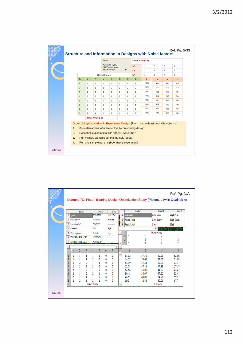
3/2/2012
112
Structure and Information in Designs with Noise fac tors
Order of Sophistication in Experiment Design (From most to least desirable options)
1. Formal treatment of noise factors by outer array design
2. Repeating experiments with "RANDOM NOISE“
3. Run multiple samples per trial (Simply repeat)
4. Run one sample per trial (Poor man's experiment)
Ref. Pg. 5-33
11 1 1 1 1 1 1
22 1 1 1 2 2 2
23 1 2 2 1 1 2
14 1 2 2 2 2 1
15 2 1 2 1 2 2
26 2 1 2 2 1 1
27 2 2 1 1 2 1
18 2 2 1 2 1 2
ETr A B - C D F
Inner Array (L-8)
Outer Array (L-4)
NC
NB
NA
1
1
1
1
2
2
2
1
3
2
1
2
4
1
2
2
R12
R22
R32
R42
R52
R62
R72
R82
R11
R21
R31
R41
R51
R61
R71
R81
R13
R23
R33
R43
R51
R63
R73
R83
R14
R24
R34
R44
R54
R64
R74
R84
Control Factors
Noise
NA:Oven Type, NB:Tempertaure, NC:Humidity �
Slide # 223
Ref. Pg. N/A
Example 7C: Piston Bearing Design Optimization Study (Piston1.q4w in Qualitek-4)
Slide # 224
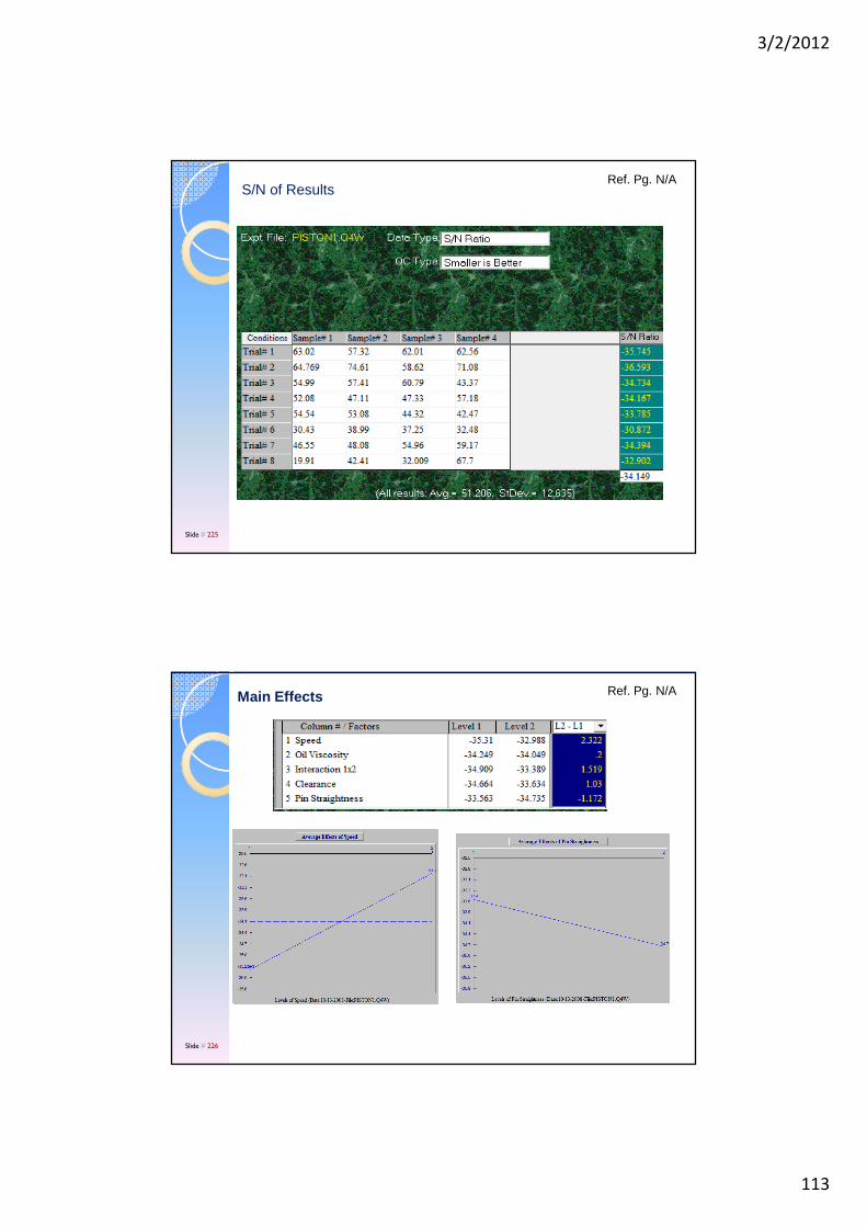
3/2/2012
113
Ref. Pg. N/AS/N of Results
Slide # 225
Ref. Pg. N/AMain Effects
Slide # 226
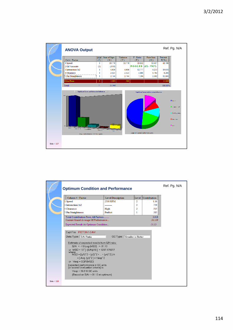
3/2/2012
114
Ref. Pg. N/AANOVA Output
Slide # 227
Ref. Pg. N/AOptimum Condition and Performance
Slide # 228
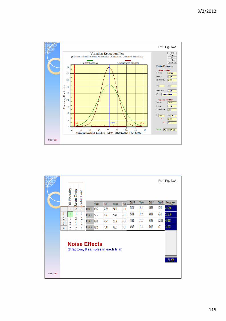
3/2/2012
115
Ref. Pg. N/A
Slide # 229
Ref. Pg. N/A
Noise Effects (3 factors, 8 samples in each trial)
Slide # 230
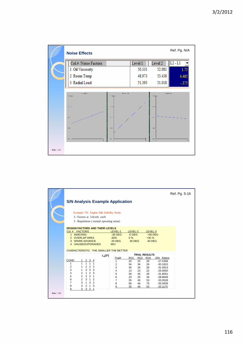
3/2/2012
116
Ref. Pg. N/ANoise Effects
Slide # 231
Example 7D: Engine Idle Stability Study
3 - Factors at 3-levels each
3 - Repetitions ( normal operating noise)
DESIGN FACTORS AND THEIR LEVELSCol. # FACTORS LEVEL-1 LEVEL-2 LEVEL-3
1 INDEXING -30 DEG O DEG +50 DEG2 OVERLAP AREA -30% 0 % +30 %3 SPARK ADVANCE 20 DEG 30 DEG 40 DEG4 UNUSED/UPGRADED M/U
CHARACTERISTIC: THE SMALLER THE BETTER
L9(34)
COND 1 2 3 41 1 1 1 12 1 2 2 23 1 3 3 34 2 1 2 35 2 2 3 1 6 2 3 1 27 3 1 3 28 3 2 1 39 3 3 2 1
TRIAL RESULTS Trial# R(1) R(2) R(3) S/N Ratios 1 20 25 26 -27.5358 2 34 36 26 -30.1815 3 45 34 26 -31.0913 4 13 23 22 -25.9550 5 36 45 35 -31.8051 6 23 25 34 -28.86497 35 45 53 -33.0528 8 56 46 75 -35.5939 9 35 46 53 -33.1175
S/N Analysis Example Application
Ref. Pg. 5-16
Slide # 232
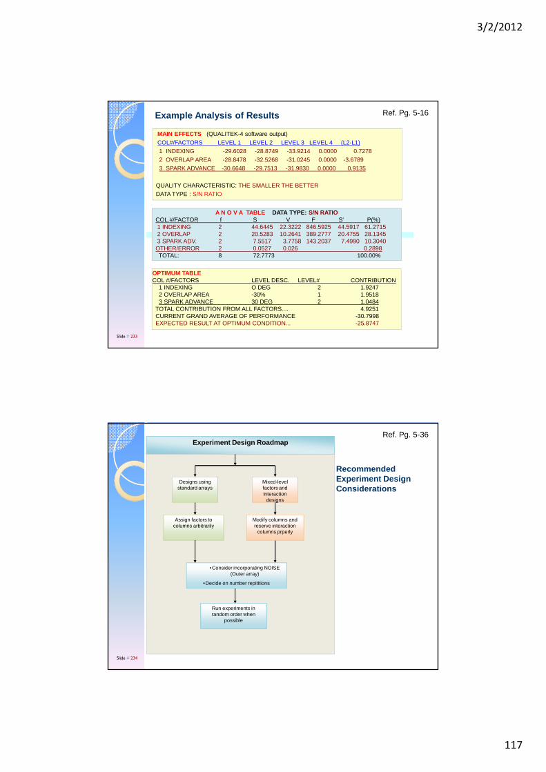
3/2/2012
117
Example Analysis of Results
MAIN EFFECTS (QUALITEK-4 software output)COL#/FACTORS LEVEL 1 LEVEL 2 LEVEL 3 LEVEL 4 (L2-L1)1 INDEXING -29.6028 -28.8749 -33.9214 0.0000 0.72782 OVERLAP AREA -28.8478 -32.5268 -31.0245 0.0000 -3.67893 SPARK ADVANCE -30.6648 -29.7513 -31.9830 0.0000 0.9135
QUALITY CHARACTERISTIC: THE SMALLER THE BETTERDATA TYPE : S/N RATIO
OPTIMUM TABLECOL #/FACTORS LEVEL DESC. LEVEL# CONTRIBUTION
1 INDEXING O DEG 2 1.92472 OVERLAP AREA -30% 1 1.95183 SPARK ADVANCE 30 DEG 2 1.0484
TOTAL CONTRIBUTION FROM ALL FACTORS.... 4.9251CURRENT GRAND AVERAGE OF PERFORMANCE -30.7998EXPECTED RESULT AT OPTIMUM CONDITION... -25.8747
A N O V A TABLE DATA TYPE: S/N RATIO COL.#/FACTOR f S V F S' P(%)1 INDEXING 2 44.6445 22.3222 846.5925 44.5917 61.27152 OVERLAP 2 20.5283 10.2641 389.2777 20.4755 28.13453 SPARK ADV. 2 7.5517 3.7758 143.2037 7.4990 10.3040OTHER/ERROR 2 0.0527 0.026 0.2898TOTAL: 8 72.7773 100.00%
Ref. Pg. 5-16
Slide # 233
Recommended Experiment Design Considerations
Ref. Pg. 5-36Experiment Design Roadmap
Designs using standard arrays
Run experiments in random order when
possible
•Consider incorporating NOISE (Outer array)
•Decide on number repititions
Assign factors to columns arbitrarily
designs
Mixed-level factors and interaction
designs
Modify columns and reserve interaction
columns prperly
Slide # 234
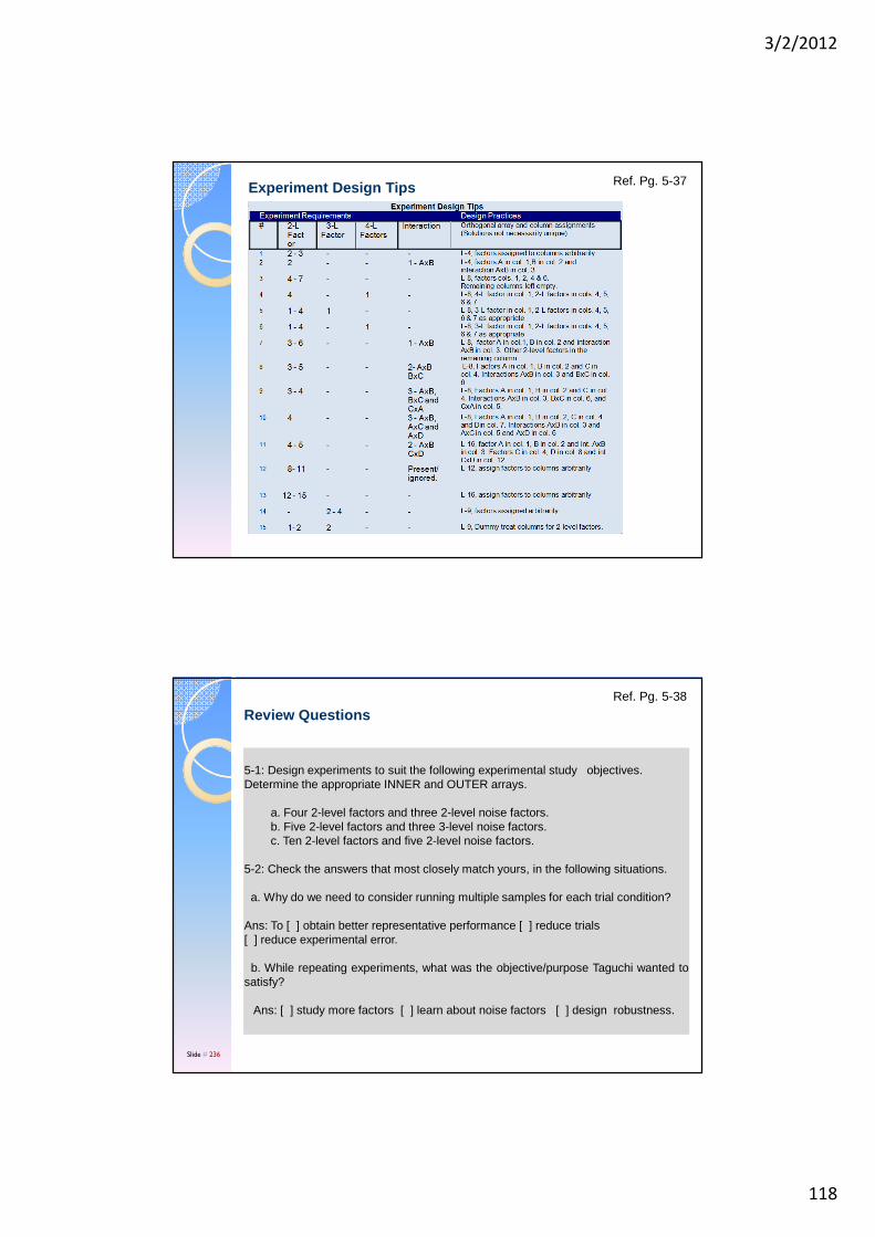
3/2/2012
118
Experiment Design Tips Ref. Pg. 5-37
5-1: Design experiments to suit the following experimental study objectives. Determine the appropriate INNER and OUTER arrays.
a. Four 2-level factors and three 2-level noise factors.b. Five 2-level factors and three 3-level noise factors.c. Ten 2-level factors and five 2-level noise factors.
5-2: Check the answers that most closely match yours, in the following situations.
a. Why do we need to consider running multiple samples for each trial condition?
Ans: To [ ] obtain better representative performance [ ] reduce trials[ ] reduce experimental error.
b. While repeating experiments, what was the objective/purpose Taguchi wanted tosatisfy?
Ans: [ ] study more factors [ ] learn about noise factors [ ] design robustness.
Review QuestionsRef. Pg. 5-38
Slide # 236

3/2/2012
119
SolveProblem 5a and 5b (40 minutes)
Recommendation: Solve problem as a group or solve individually and discuss with your TEAM member.
Note: Install Qualitek-4 software (if asked) using Reg.# 409240108100690. Remove software after class.
Ref. Page 5-42
Slide # 237
Practice and Learn
Practice Problem # 5A: Practice Problem # 5A:
Ref. Page 5-42
Slide # 238
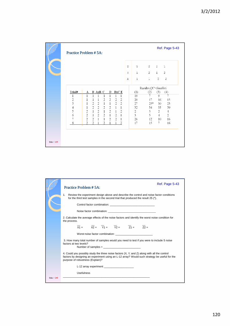
3/2/2012
120
Practice Problem # 5A: Practice Problem # 5A: Ref. Page 5-43
Slide # 239
Practice Problem # 5A: Practice Problem # 5A:
1. Review the experiment design above and describe the control and noise factor conditions for the third test samples in the second trial that produced the result 25 (*).
Control factor combination: ______________________________
Noise factor combination: ________________________________
2. Calculate the average effects of the noise factors and identify the worst noise condition for the process.
__ __ __ __ __ __X1 = X2 = Y1 = Y2 = Z1 = Z2 =
Worst noise factor combination: _________________________
3. How many total number of samples would you need to test if you were to include 5 noise factors at two levels?
Number of samples = _________________________
4. Could you possibly study the three noise factors (X, Y, and Z) along with all the control factors by designing an experiment using an L-12 array? Would such strategy be useful for the purpose of robustness (Explain)?
L-12 array experiment ____________________
Usefulness __________________________________________________________
Ref. Page 5-43
Slide # 240
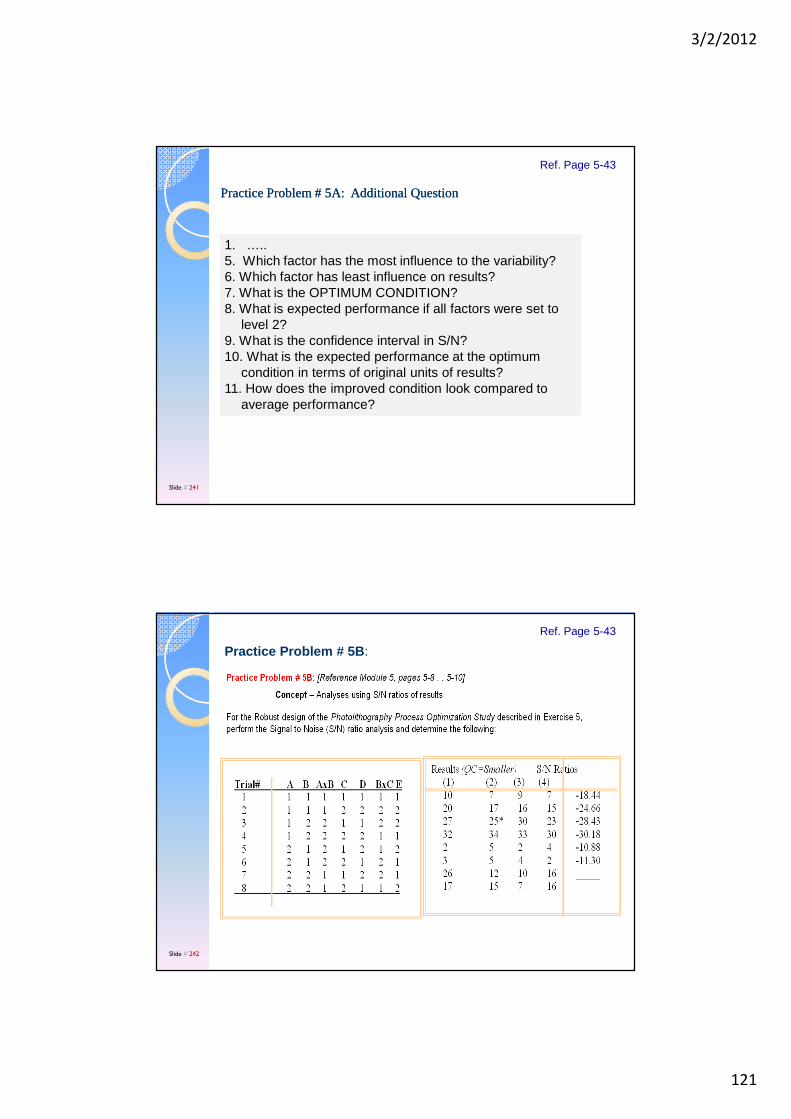
3/2/2012
121
Practice Problem # 5A: Additional QuestionPractice Problem # 5A: Additional Question
1. ….. 5. Which factor has the most influence to the variability?6. Which factor has least influence on results?7. What is the OPTIMUM CONDITION?8. What is expected performance if all factors were set to
level 2? 9. What is the confidence interval in S/N?10. What is the expected performance at the optimum
condition in terms of original units of results?11. How does the improved condition look compared to
average performance?
Ref. Page 5-43
Slide # 241
Practice Problem # 5B :
Ref. Page 5-43
Slide # 242
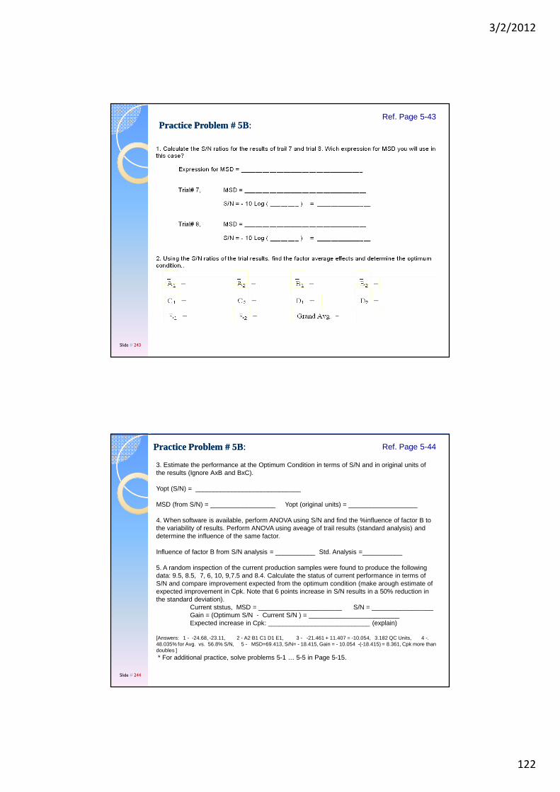
3/2/2012
122
Practice Problem # 5BPractice Problem # 5B: : Ref. Page 5-43
Slide # 243
Practice Problem # 5BPractice Problem # 5B: :
3. Estimate the performance at the Optimum Condition in terms of S/N and in original units of the results (Ignore AxB and BxC).
Yopt (S/N) = _____________________________
MSD (from S/N) = __________________ Yopt (original units) = ___________________
4. When software is available, perform ANOVA using S/N and find the %influence of factor B to the variability of results. Perform ANOVA using aveage of trail results (standard analysis) and determine the influence of the same factor.
Influence of factor B from S/N analysis = ___________ Std. Analysis =___________
5. A random inspection of the current production samples were found to produce the following data: 9.5, 8.5, 7, 6, 10, 9,7.5 and 8.4. Calculate the status of current performance in terms of S/N and compare improvement expected from the optimum condition (make arough estimate of expected improvement in Cpk. Note that 6 points increase in S/N results in a 50% reduction in the standard deviation).
Current ststus, MSD = _______________________ S/N = _________________Gain = (Optimum S/N - Current S/N ) = _________________________Expected increase in Cpk: ____________________________ (explain)
[Answers: 1 - -24.68, -23.11, 2 - A2 B1 C1 D1 E1, 3 - -21.461 + 11.407 = -10.054, 3.182 QC Units, 4 -. 48.035% for Avg. vs. 56.8% S/N, 5 - MSD=69.413, S/N= - 18.415, Gain = - 10.054 -(-18.415) = 8.361, Cpk more than doubles ]
* For additional practice, solve problems 5-1 … 5-5 in Page 5-15.
Ref. Page 5-44
Slide # 244
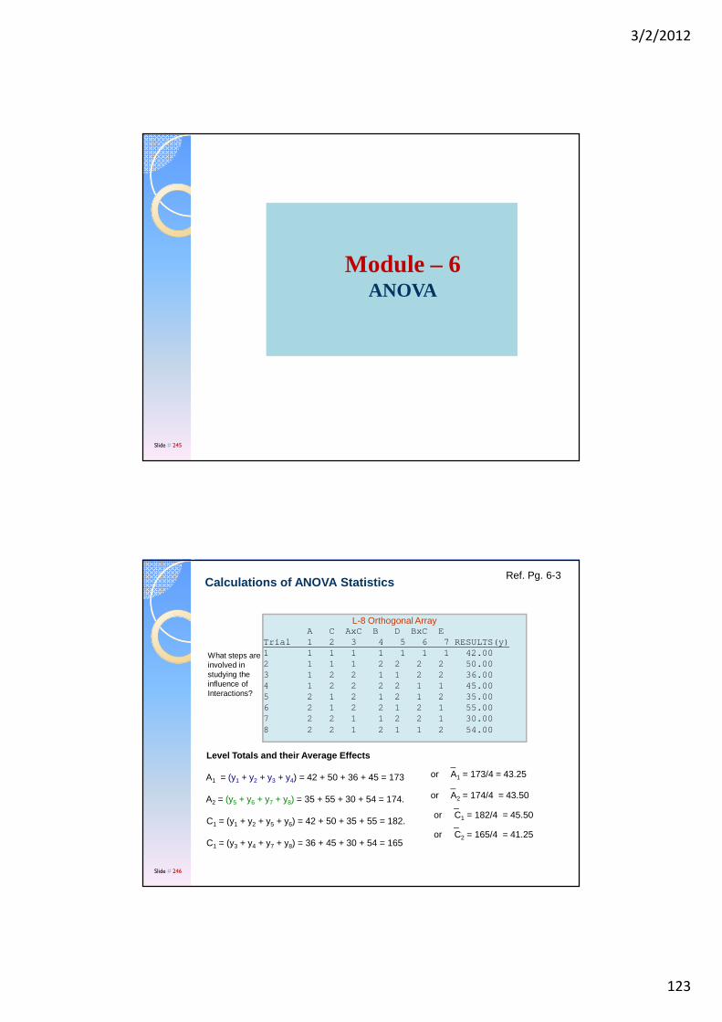
3/2/2012
123
Module – 6ANOVA
Slide # 245
What steps are involved in studying the influence of Interactions?
L-8 Orthogonal ArrayA C AxC B D BxC E
Trial 1 2 3 4 5 6 7 RESULTS(y)1 1 1 1 1 1 1 1 42.00 2 1 1 1 2 2 2 2 50.00 3 1 2 2 1 1 2 2 36.00 4 1 2 2 2 2 1 1 45.00 5 2 1 2 1 2 1 2 35.00 6 2 1 2 2 1 2 1 55.00 7 2 2 1 1 2 2 1 30.00 8 2 2 1 2 1 1 2 54.00
_or A1 = 173/4 = 43.25
_or A2 = 174/4 = 43.50
_or C1 = 182/4 = 45.50
_or C2 = 165/4 = 41.25
Level Totals and their Average Effects
A1 = (y1 + y2 + y3 + y4) = 42 + 50 + 36 + 45 = 173
A2 = (y5 + y6 + y7 + y8) = 35 + 55 + 30 + 54 = 174.
C1 = (y1 + y2 + y5 + y6) = 42 + 50 + 35 + 55 = 182.
C1 = (y3 + y4 + y7 + y8) = 36 + 45 + 30 + 54 = 165
Calculations of ANOVA StatisticsRef. Pg. 6-3
Slide # 246
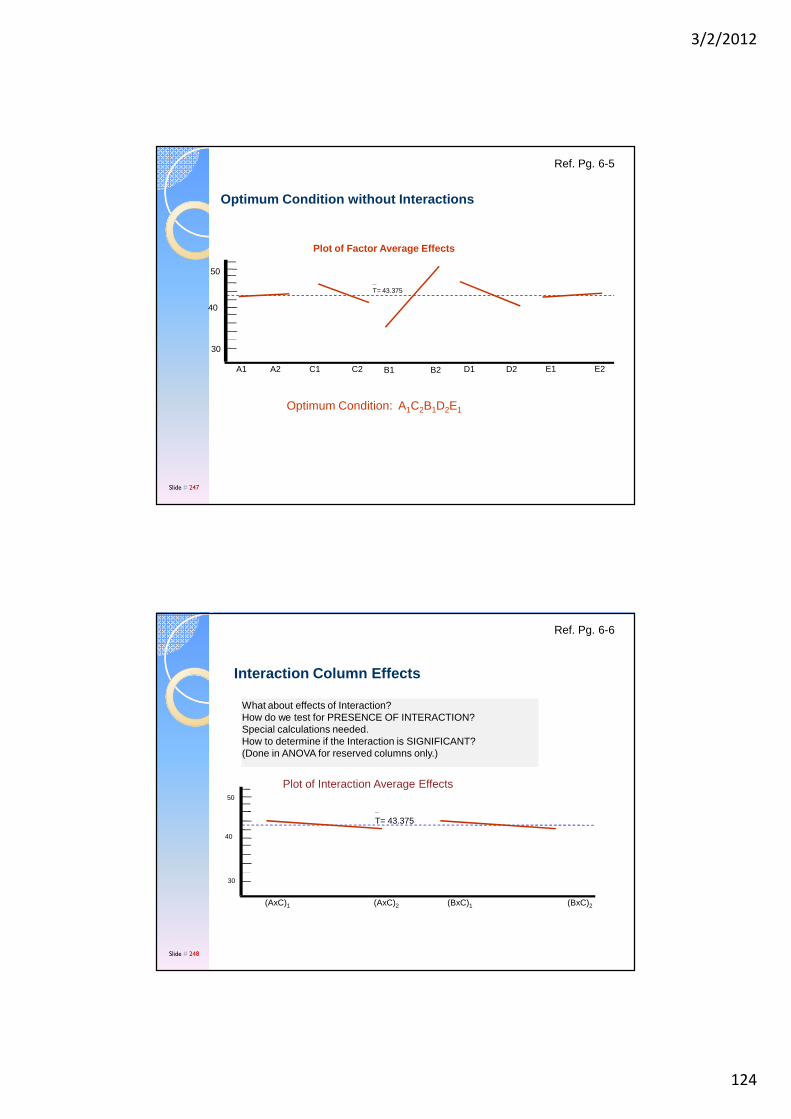
3/2/2012
124
A1 A2 D1 D2C1 C2 B1 B2 E1 E2
30
40
50
T= 43.375_
Plot of Factor Average Effects
Optimum Condition: A1C2B1D2E1
Optimum Condition without Interactions
Ref. Pg. 6-5
Slide # 247
What about effects of Interaction?How do we test for PRESENCE OF INTERACTION?Special calculations needed.How to determine if the Interaction is SIGNIFICANT?(Done in ANOVA for reserved columns only.)
(AxC)1 (AxC)2 (BxC)1 (BxC)2
30
40
50
T= 43.375_
Plot of Interaction Average Effects
Interaction Column Effects
Ref. Pg. 6-6
Slide # 248
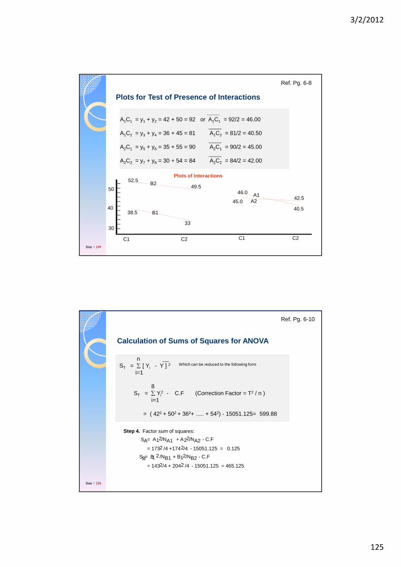
3/2/2012
125
____A1C1 = y1 + y2 = 42 + 50 = 92 or A1C1 = 92/2 = 46.00
____A1C2 = y3 + y4 = 36 + 45 = 81 A1C2 = 81/2 = 40.50
____ A2C1 = y5 + y6 = 35 + 55 = 90 A2C1 = 90/2 = 45.00
____A2C2 = y7 + y8 = 30 + 54 = 84 A2C2 = 84/2 = 42.00
C1 C2
30
40
50
Plots of Interactions
C1 C2
52.549.5
38.5
33
B2
46.0
B1
45.040.5
42.5A1
A2
Plots for Test of Presence of Interactions
Ref. Pg. 6-8
Slide # 249
Step 4. Factor sum of squares:
SA= A12/NA1 + A22/NA2 - C.F
= 1732 /4 +1742/4 - 15051.125 = 0.125
SB= B1 2 /NB1 + B12/NB2 - C.F
= 1432 /4 + 2042 /4 - 15051.125 = 465.125
Calculation of Sums of Squares for ANOVA
n __ST = ∑ [ Yi - Y ] 2 Which can be reduced to the following form
i=1
8ST = ∑ Yi
2 - C.F (Correction Factor = T2 / n )i=1
= ( 422 + 502 + 362+ ..... + 542) - 15051.125= 599.88
Ref. Pg. 6-10
Slide # 250

3/2/2012
126
A1 = 8 A2 = 8B1 =5 B2 = 11C1 = 9 C2 = 7
Avg. = 4,ST = 10, CF = 64
SA = 64/2 + 64/2 – 64 =0SB = 25/2 + 121/2 – 64 = 9SC = 81/2 + 49/2 – 65 = 1
L-4 Orthogonal ArrayTrial #A B C Result1 1 1 1 32 1 2 2 53 2 1 2 24 2 2 1 6
An Example Data for ANOVA
Ref. Page N/A
Slide # 251
Se = ST - ( SA + SB + SC + SD + SE +SAxC + SBxC )
= 599.88 - 599.88 = 0
Step 5. Experiment Degrees of Freedom
fT = n - 1 = 8 - 1 = 7 (Total number of results - 1)
fe = fT - ( fA + fB+ fC + fD +fE +fAxC + fBxC ) = 0
Step 6. factor degrees of freedom
fA = (# levels of factor A) - 1 = 2 - 1 = 1
fB = (# levels of factor B) - 1 = 2 - 1 = 1
How is Variance calculated?VA = SA /fA = 0.125 / 1 = 0.125VB = SB /fB = 465.125 / 1 = 465.125
How is F-ratios calculated?
How is PUR SUMS OF SQUARES calculated?
How is percent INFLUENCE calculated?
PA = SA/ST = 0.125/ 599.88 = 0.02%
PB = SB/ST = 465.125/ 599.88 = 77.54%
Calculations of Error Terms and & DOF
Ref. Pg. 6-12
Slide # 252
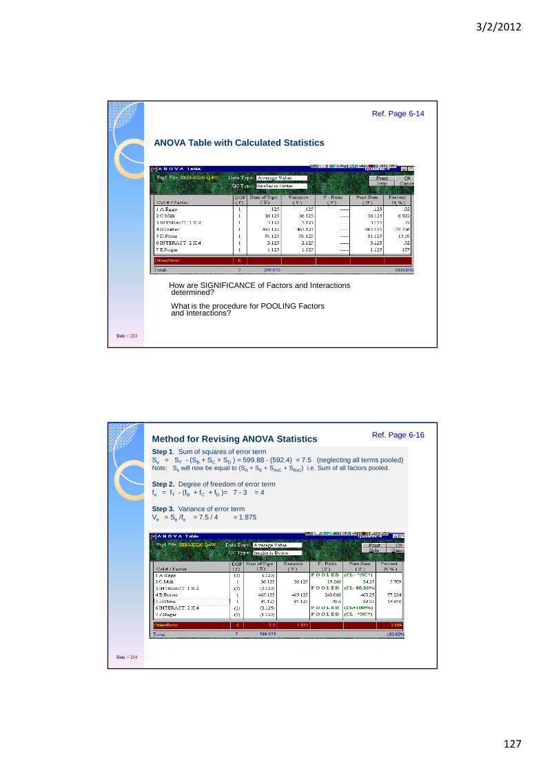
3/2/2012
127
How are SIGNIFICANCE of Factors and Interactionsdetermined?
What is the procedure for POOLING Factorsand Interactions?
ANOVA Table with Calculated Statistics
Ref. Page 6-14
Slide # 253
Step 1 . Sum of squares of error termSe = ST - (SB + SC + SD ) = 599.88 - (592.4) = 7.5 (neglecting all terms pooled)Note: Se will now be equal to (SA + SE + SAxC + SBxC) i.e. Sum of all factors pooled.
Step 2. Degree of freedom of error termfe = fT - (fB + fC + fD )= 7 - 3 = 4
Step 3. Variance of error termVe = Se /fe = 7.5 / 4 = 1.875
Method for Revising ANOVA Statistics Ref. Page 6-16
Slide # 254

3/2/2012
128
Slide # 255
Is factor C significant? Should we pool factor C ?
To study the possibility of pooling, is to perform test of significance for factor C. The significance test is carried out by comparing the experiment F-ratio with the standard table value for a desired Confidence Level (subjective: 90, 95 or 99% commonly used).
From the ANOVA table FC = 19.267 (From Experiment)
From The F-TABLE, Find F Value At n1 = DOF OF Factor C = 1n2 = DOF Of Error Term = 4 At A Confidence Level (say 95%) .
F (table) = 7.7086 (From F-Table)
Since FC Is Greater Than the F(table),Factor C should not be pooled .
Recommendations: Create non-zero DOF for the error term by pooling the weaker factors. Test for significance first, then pool. Attempt to pool until the DOF for the error term is about half the experiment DOF.
Performing Test of Significance for Pooling
Ref. Page 6-17
Slide # 256
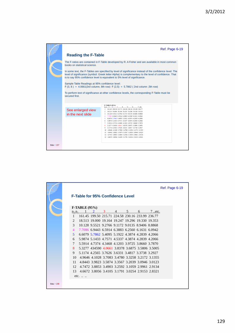
3/2/2012
129
The F-ratios are contained in F-Table developed by R. A Fisher and are available in most common books on statistical science.
In some text, the F-Tables are specified by level of significance instead of the confidence level. The level of significance (symbol: Greek letter Alpha) is complementary to the level of confidence. That is to say 95% confidence level is equivalent to 5% level of significance.
Sample Table Readings at 95% confidence level: F (3, 8 ) = 4.0661(3rd column, 8th row) F (2,5) = 5.7862 ( 2nd column ,5th row)
To perform test of significance at other confidence levels, the corresponding F-Table must be secured first.
F-TABLE (95%)n2\n1 1 2 3 4 5 6 7 ..etc.
1 161.45 199.50 215.71 224.58 230.16 233.99 236.77
2 18.513 19.000 19.164 19.247 19.296 19.330 19.353
3 10.128 9.5521 9.2766 9.1172 9.0135 8.9406 8.8868
4 7.70866.9443 6.5914 6.3883 6.2560 6.1631 6.0942
5 6.6079 5.7862 5.4095 5.1922 4.3874 4.2839 4.2066
6 5.9874 5.1433 4.7571 4.5337 4.3874 4.2839 4.2066
7 5.5914 4.7374 4.3468 4.1203 3.9725 3.8660 3.7870
8 5.3277 4.3459 4.0661 3.8378 3.6875 3.5806 3.5005
9 5.1174 4.2565 3.7626 3.6331 3.4817 3.3738 3.2927
10 4.9646 4.1028 3.7083 3.4780 3.3258 3.2172 3.1355
11 4.8443 3.9823 3.5874 3.3567 3.2039 3.0946 3.0123
12 4.7472 3.8853 3.4903 3.2592 3.1059 2.9961 2.9134
13 4.6672 3.8056 3.4105 3.1791 3.0254 2.9153 2.8321
See enlarged view in the next slide
Reading the F-Table
Ref. Page 6-19
Slide # 257
F-TABLE (95%)n2\n1 1 2 3 4 5 6 7 ..etc.1 161.45 199.50 215.71 224.58 230.16 233.99 236.77 2 18.513 19.000 19.164 19.247 19.296 19.330 19.353 3 10.128 9.5521 9.2766 9.1172 9.0135 8.9406 8.8868 4 7.70866.9443 6.5914 6.3883 6.2560 6.1631 6.09425 6.6079 5.7862 5.4095 5.1922 4.3874 4.2839 4.2066 6 5.9874 5.1433 4.7571 4.5337 4.3874 4.2839 4.2066 7 5.5914 4.7374 4.3468 4.1203 3.9725 3.8660 3.7870 8 5.3277 434590 4.0661 3.8378 3.6875 3.5806 3.5005 9 5.1174 4.2565 3.7626 3.6331 3.4817 3.3738 3.2927 10 4.9646 4.1028 3.7083 3.4780 3.3258 3.2172 3.1355 11 4.8443 3.9823 3.5874 3.3567 3.2039 3.0946 3.0123 12 4.7472 3.8853 3.4903 3.2592 3.1059 2.9961 2.9134 13 4.6672 3.8056 3.4105 3.1791 3.0254 2.9153 2.8321 etc. .. ..
F-Table for 95% Confidence Level
Ref. Page 6-19
Slide # 258
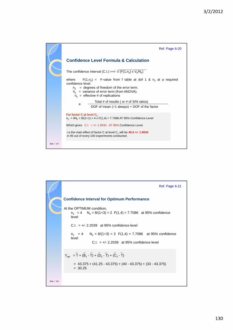
3/2/2012
130
For factor C at level C 1n2 = 4Ne = 8/(1+1) = 4 x F(1,4) = 7.7086 AT 95% Confidence Level
Which gives C.I. = +/- 1.9034 AT 95% Confidence Level.
i.e the main effect of factor C at level C1 will be 45.5 +/- 1.9034in 95 out of every 100 experiments conducted.
The confidence interval (C.I.) =+/- \/ (F(1,n2) x Ve/Ne)
where F(1,n2) = F-value from f table at dof 1 & n2 at a requiredconfidence level.
n2 = degrees of freedom of the error term.Ve = variance of error term (from ANOVA).ne = effective # of replications
= DOF of mean (=1 always) + DOF of the factor
Total # of results ( or # of S/N ratios)
Confidence Level Formula & Calculation
Ref. Page 6-20
Slide # 259
At the OPTIMUM condition,n2 = 4 Ne = 8/(1+3) = 2 F(1,4) = 7.7086 at 95% confidence level
C.I. = +/- 2.2039 at 95% confidence level
n2 = 4 Ne = 8/(1+3) = 2 F(1,4) = 7.7086 at 95% confidencelevel
C.I. = +/- 2.2039 at 95% confidence level
__Grand average of performance: T = 347 / 8 = 43.375
_ _ _ _ _ _ _Yopt = T + (B1 - T) + (D2 - T) + (C2 - T)
= 43.375 + (41.25 - 43.375) + (40 - 43.375) + (33 - 43.375)= 30.25
Confidence Interval for Optimum Performance
Ref. Page 6-21
Slide # 260
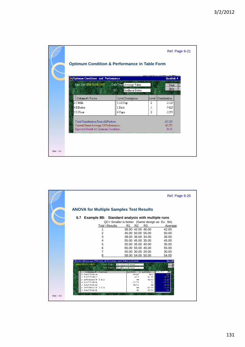
3/2/2012
131
Optimum Condition & Performance in Table Form
Ref. Page 6-21
Slide # 261
6.7 Example 8B: Standard analysis with multiple runsQC= Smaller is better (Same design as Ex. 8A)
Trial \ Results R1 R2 R3 Average1 38.00 42.00 46.00 42.002 45.00 50.00 55.00 50.003 38.00 36.00 34.00 36.004 55.00 45.00 35.00 45.005 30.00 35.00 40.00 35.006 65.00 55.00 45.00 55.007 40.00 30.00 20.00 30.008 58.00 54.00 50.00 54.00
ANOVA for Multiple Samples Test Results
Ref. Page 6-25
Slide # 262

3/2/2012
132
DOF = 8 x 3 - 1 = 23B1 = (38.0 + 42.0 + 46.0) + (38.0 + 36.0 + 34.0)
+ (30.0 + 35.0 + 40.0) + (40.0 + 30.0 + 20.0) = 429
Note: B1 is obtained from results of trial conditions 1, 3, 5 & 7.
DOF with Multiple Samples Test Results
Ref. Page 6-26
Slide # 263
ANOVA Screen After Pooling Insignificant Factors
Ref. Page 6-27
Slide # 264
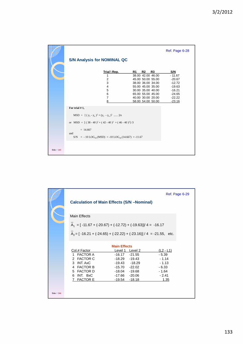
3/2/2012
133
For trial # 1,
MSD = [ ( y1 - yo )2 + (y2 - yo )2 ...... ]/n
or MSD = [ ( 38 - 40 )2 + ( 42 - 40 )2 + ( 46 - 40 )2] /3
= 14.667and
S/N = - 10 LOG10 (MSD) = -10 LOG10 (14.667) = -11.67
Trial \ Rep. R1 R2 R3 S/N1 38.00 42.00 46.00 - 11.672 45.00 50.00 55.00 -20.673 38.00 36.00 34.00 -12.724 55.00 45.00 35.00 -19.635 30.00 35.00 40.00 -16.216 65.00 55.00 45.00 -24.657 40.00 30.00 20.00 -22.228 58.00 54.00 50.00 -23.16
S/N Analysis for NOMINAL QC
Ref. Page 6-28
Slide # 265
Main Effects_A1 = [ -11.67 + (-20.67) + (-12.72) + (-19.63)]/ 4 = -16.17_A2 = [ -16.21 + (-24.65) + (-22.22) + (-23.16)] / 4 = -21.55, etc.
Main EffectsCol.# Factor Level 1 Level 2 (L2 - L1)1 FACTOR A -16.17 -21.55 - 5.392 FACTOR C -18.29 -19.43 - 1.143 INT. AxC -19.43 -18.29 - 1.134 FACTOR B -15.70 -22.02 - 6.335 FACTOR D -18.04 -19.68 - 1.646 INT. BxC -17.66 -20.06 - 2.417 FACTOR E -19.54 -18.18 1.35
Calculation of Main Effects (S/N –Nominal)
Ref. Page 6-29
Slide # 266
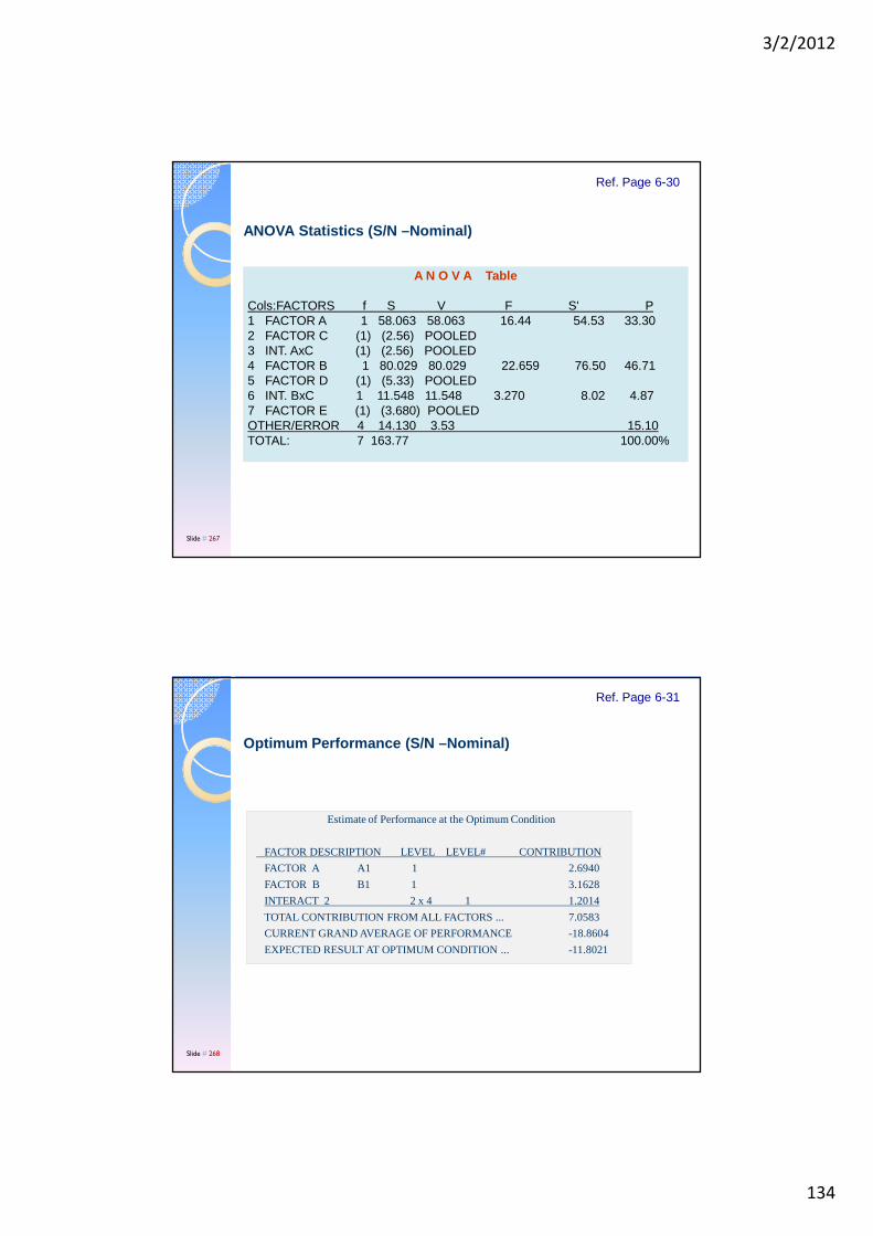
3/2/2012
134
A N O V A Table
Cols:FACTORS f S V F S' P1 FACTOR A 1 58.063 58.063 16.44 54.53 33.302 FACTOR C (1) (2.56) POOLED3 INT. AxC (1) (2.56) POOLED4 FACTOR B 1 80.029 80.029 22.659 76.50 46.715 FACTOR D (1) (5.33) POOLED6 INT. BxC 1 11.548 11.548 3.270 8.02 4.877 FACTOR E (1) (3.680) POOLEDOTHER/ERROR 4 14.130 3.53 15.10TOTAL: 7 163.77 100.00%
ANOVA Statistics (S/N –Nominal)
Ref. Page 6-30
Slide # 267
Estimate of Performance at the Optimum Condition
FACTOR DESCRIPTION LEVEL LEVEL# CONTRIBUTION
FACTOR A A1 1 2.6940
FACTOR B B1 1 3.1628
INTERACT 2 2 x 4 1 1.2014
TOTAL CONTRIBUTION FROM ALL FACTORS ... 7.0583
CURRENT GRAND AVERAGE OF PERFORMANCE -18.8604
EXPECTED RESULT AT OPTIMUM CONDITION ... -11.8021
Optimum Performance (S/N –Nominal)
Ref. Page 6-31
Slide # 268
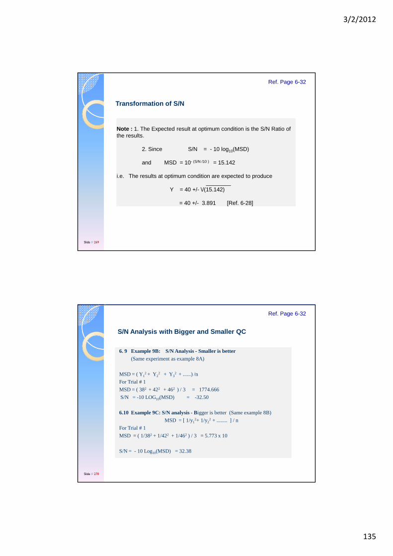
3/2/2012
135
Note : 1. The Expected result at optimum condition is the S/N Ratio of the results.
2. Since S/N = - 10 log10(MSD)
and MSD = 10- (S/N /10 ) = 15.142
i.e. The results at optimum condition are expected to produce________
Y = 40 +/- \/(15.142)
= 40 +/- 3.891 [Ref. 6-28]
Transformation of S/N
Ref. Page 6-32
Slide # 269
6. 9 Example 9B: S/N Analysis - Smaller is better
(Same experiment as example 8A)
MSD = ( Y12 + Y2
2 + Y32 + ......) /n
For Trial # 1
MSD = ( 382 + 422 + 462 ) / 3 = 1774.666
S/N = -10 LOG10(MSD) = -32.50
6.10 Example 9C: S/N analysis - Bigger is better (Same example 8B)
MSD = [ 1/y12+ 1/y22 + ........ ] / n
For Trial # 1
MSD = ( 1/382 + 1/422 + 1/462 ) / 3 = 5.773 x 10
S/N = - 10 Log10(MSD) = 32.38
S/N Analysis with Bigger and Smaller QC
Ref. Page 6-32
Slide # 270
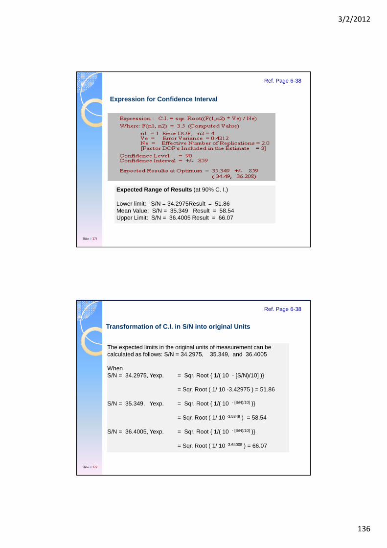
3/2/2012
136
Expected Range of Results (at 90% C. I.)
Lower limit: S/N = 34.2975Result = 51.86Mean Value: S/N = 35.349 Result = 58.54Upper Limit: S/N = 36.4005 Result = 66.07
Expression for Confidence Interval
Ref. Page 6-38
Slide # 271
The expected limits in the original units of measurement can be calculated as follows: S/N = 34.2975, 35.349, and 36.4005
WhenS/N = 34.2975, Yexp. = Sqr. Root { 1/( 10 - [S/N)/10] )}
= Sqr. Root ( 1/ 10 -3.42975 ) = 51.86
S/N = 35.349, Yexp. = Sqr. Root { 1/( 10 - [S/N)/10] )}
= Sqr. Root ( 1/ 10 -3.5349 ) = 58.54
S/N = 36.4005, Yexp. = Sqr. Root { 1/( 10 - [S/N)/10] )}
= Sqr. Root ( 1/ 10 -3.64005 ) = 66.07
Transformation of C.I. in S/N into original Units
Ref. Page 6-38
Slide # 272

3/2/2012
137
Trials
Array
Runs
6.11 Understanding and Interpreting Error Terms(Signature Plots)
1. Is the experiment satisfactory?
2. What if the confirmation is unsatisfactory?
3. When should you consider repeating the experimentfrom the start?
Relationship between the Results and the Error Term
Ref. Page 6-39
Slide # 273
6-1: What does it mean when ANOVA indicates a high percentage of influence (P6-1: What does it mean when ANOVA indicates a high percentage of influence (Pe= 30%, 60% or 80%; fe > 0)? Check all appropriate answers.
a. ( ) It shows the experiment was poorly conducted and shouldbe repeated.b. ( ) It does not necessarily indicate that the experiment was bad.c. ( ) It indicates that the performance of the product/process is largely
influenced by factors not included in the study.d. ( ) It means that the results at the same trial condition varies significantly
when repeated.e. ( ) It means that the results vary extensively from trial condition to trial
condition.
6-2: How do you determine when and what factors to `pool'? Check all correctanswers.
a. ( ) Pool all factors which fail the test for significance (say 95% confidence).b. ( ) Start pooling with the factor that has the least % influence (Pe).c. ( ) There is no general % guideline for pooling. It depends on several factors.d. ( ) You should always attempt to pool if error DOF = 0.e. ( ) In general, try to pool until the error DOF is about half the total DOF.
Review Questions
Ref. Page 6-42
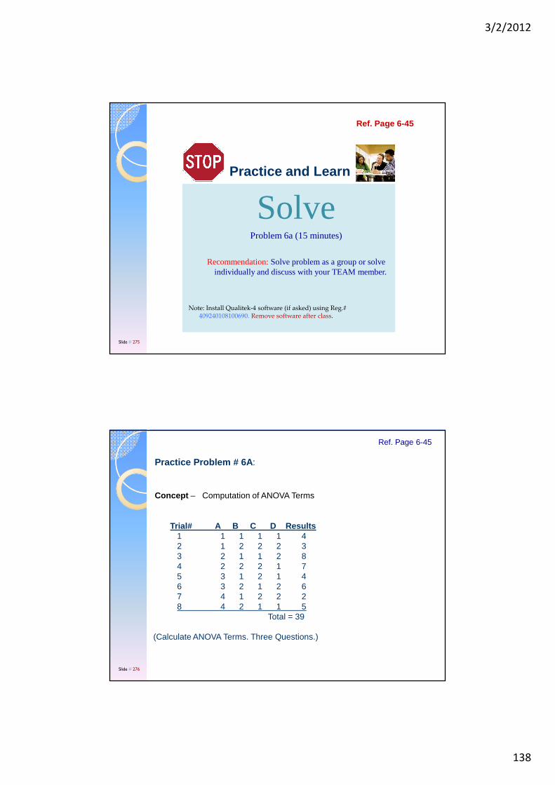
3/2/2012
138
SolveProblem 6a (15 minutes)
Recommendation: Solve problem as a group or solve individually and discuss with your TEAM member.
Note: Install Qualitek-4 software (if asked) using Reg.# 409240108100690. Remove software after class.
Ref. Page 6-45
Slide # 275
Practice and Learn
Concept – Computation of ANOVA Terms
Trial# A B C D Results1 1 1 1 1 42 1 2 2 2 33 2 1 1 2 84 2 2 2 1 75 3 1 2 1 46 3 2 1 2 67 4 1 2 2 28 4 2 1 1 5
Total = 39
(Calculate ANOVA Terms. Three Questions.)
Practice Problem # 6A :
Ref. Page 6-45
Slide # 276

3/2/2012
139
Jokes for the day . .Jokes for the day . .This is the transcript of the ACTUAL radio conversation of a US Naval ship and the Canadians, off the coast of Newfoundland, Oct 95, released by the Chief of Naval
Operations 10-10-95.
Canadians:Please divert your course 15 degrees to the South, to avoid a collision.Americans:Recommend you divert your course 15 degrees to the North, to avoid a
collision.Canadians:Negative. You will have to divert your course 15 degrees to the South to
avoid a collision.Americans:This is the Captain of a US Navy ship. I say again, divert YOUR course.Canadians:Negative. I say again, You will have to divert your course.Americans:This is the aircraft carrier USS Lincoln. The second largest ship in the
United States Atlantic Fleet, we are accompanied by three destroyers, three cruisers, and numerous support vessels. I demand that you change your course 15 degrees north, I say again, that's 15 degrees north, or countermeasures will be undertaken to ensure the safety of this ship.
Canadians:We are a lighthouse. Your call.
Slide # 277
Module – 7Loss Function
Slide # 278
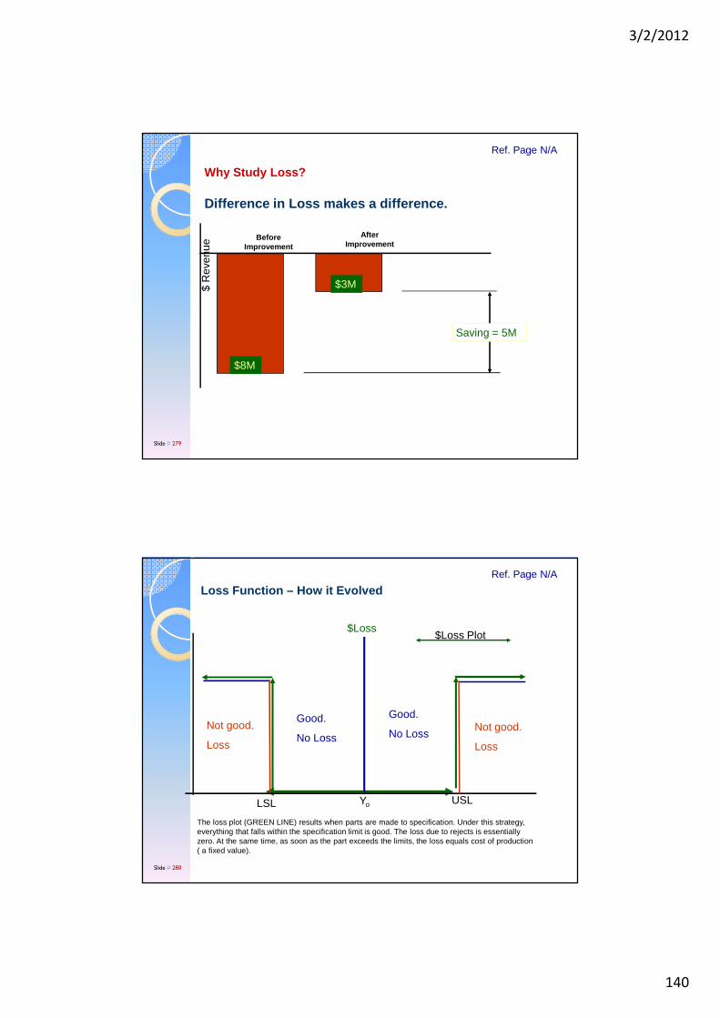
3/2/2012
140
Why Study Loss?
Difference in Loss makes a difference.
Ref. Page N/A
$8M
$3M$ R
even
ue
After Improvement
Before Improvement
Saving = 5M
Slide # 279
Loss Function – How it EvolvedRef. Page N/A
Yo
Not good.
Loss
USL LSL
Not good.
Loss
Good.
No LossGood.
No Loss
$Loss $Loss Plot
The loss plot (GREEN LINE) results when parts are made to specification. Under this strategy, everything that falls within the specification limit is good. The loss due to rejects is essentially zero. At the same time, as soon as the part exceeds the limits, the loss equals cost of production ( a fixed value).
Slide # 280
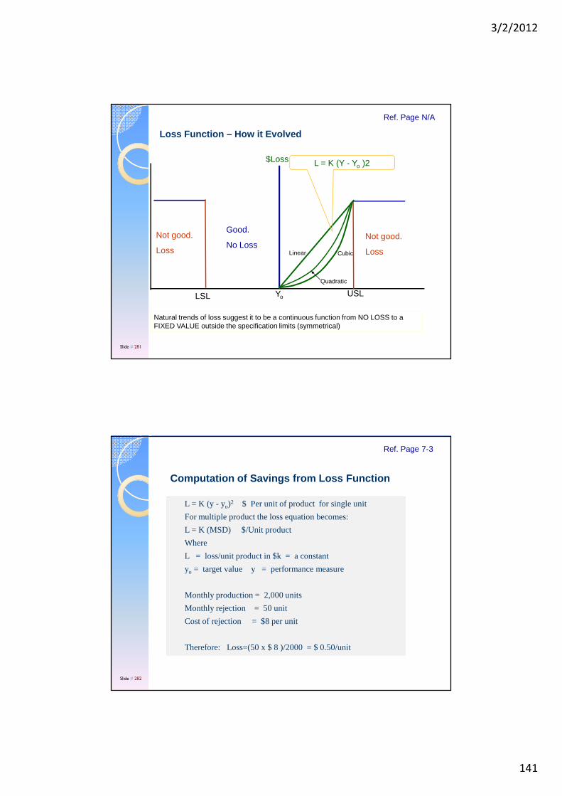
3/2/2012
141
Loss Function – How it Evolved
Ref. Page N/A
Yo
Not good.
Loss
USL LSL
Not good.
Loss
Good.
No Loss
$Loss
Natural trends of loss suggest it to be a continuous function from NO LOSS to a FIXED VALUE outside the specification limits (symmetrical)
Linear
Quadratic
Cubic
L = K (Y - Yo )2
Slide # 281
L = K (y - yo)2 $ Per unit of product for single unit
For multiple product the loss equation becomes:
L = K (MSD) $/Unit product
Where
L = loss/unit product in $k = a constant
yo = target value y = performance measure
Monthly production = 2,000 units
Monthly rejection = 50 unit
Cost of rejection = $8 per unit
Therefore: Loss=(50 x $ 8 )/2000 = $ 0.50/unit
Computation of Savings from Loss Function
Ref. Page 7-3
Slide # 282

3/2/2012
142
Input for Saving Computation from Loss Function
Ref. Page 7-4
Slide # 283
Find Monthly SavingsLoss Function, L = K (Y-Yo)2 For a single unit.Thus
20 = K (Yo +/- TOL - Yo)2
(since, when y = yo +/- TOL, all parts are rejected andthe loss equals cost of rejecting a single unit)
or 20 = K (TOL)2
or K = 20/(TOL)2 = 20/(.35)2 = 163.265Also, L = K (MSD) for the population of parts
Loss Function Manipulation
Ref. Page 7-5
Slide # 284

3/2/2012
143
Loss Before Experiment/Current DesignL = K (MSD) = 163.265 x .0475) = $ 7.75
Loss After Experiment/New DesignL = K (MSD) = 163.265 x .0145) = $ 2.36
BEFORES/N = 13.23307
OR MSD = .0475
AFTER S/N = 18.38631
OR MSD = 0.0145
Savings Per Month = 7.75 - 2.36 = $ 5.39/PER PRODUCT
Total Savings Per Month = 15000 x 5.39 = $ 80,850
Expected Savings from the Improvement
Ref. Page 7-6
Slide # 285
Normal DistributionAmong several distribution equations, most widely used is the Normal Distribution which was discovered by Gauss, Laplace and Demoivre, independently. But it is generally identified as Gaussian distribution or the Gaussian error law .
Where, x is the random variable, f(x) probability of x ( -∞ <= x <= + ∞ ) and µ = average (Mean) of population, σσσσ = standard deviation of population
1
σσσσ 2 Πf(x) = e( x - µµµµ ) 2
2 σ2
Mathematical Expression for Normal Distribution
Ref. Page 7-7
Slide # 286

3/2/2012
144
When S/N is given, MSD can be calculated MSD = 10 -[(S/N)/10]
also, since MSD = σ2 + (a - yo )
2 a = sample average and yo = Target value Standard deviation, σσσσ can also be calculated when a and yo are known or assumed.
Improvements Expressed in terms of Reduced Variatio n
Ref. Page 7-8
Slide # 287
Since MSD = 10 -[(S/N)/10]
and MSD = σ2 + (a - yo )2 = σ2 when average is on target
σ improved = σ current { (MSD)improved /(MSD)current}0.5
σσσσ improved = σσσσ current 10
(Above equation should apply to all three quality characteristics)
[(S/N)current - (S/N)imprved]20
99.73 %95.45 %68.27 %
1σ-1σ 2σ-2σ 3σ-3σ
Area under Normal Distribution
Savings from Known Improvement in S/N
Ref. Page 7-11
Slide # 288
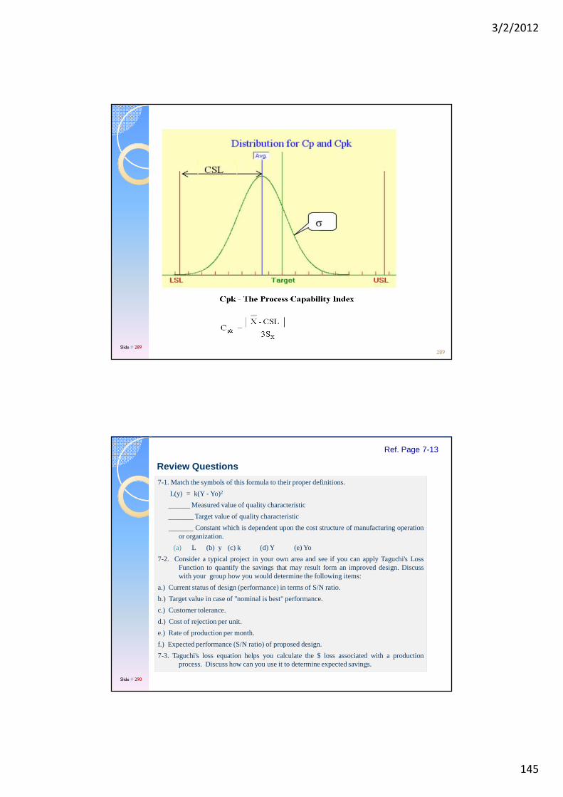
3/2/2012
145
289Slide # 289
7-1. Match the symbols of this formula to their proper definitions.
L(y) = k(Y - Yo)2
______ Measured value of quality characteristic
_______ Target value of quality characteristic
_______ Constant which is dependent upon the cost structureof manufacturing operationor organization.
(a) L (b) y (c) k (d) Y (e) Yo
7-2. Consider a typical project in your own area and see if youcan apply Taguchi's LossFunction to quantify the savings that may result form an improved design. Discusswith your group how you would determine the following items:
a.) Current status of design (performance) in terms of S/N ratio.
b.) Target value in case of "nominal is best" performance.
c.) Customer tolerance.
d.) Cost of rejection per unit.
e.) Rate of production per month.
f.) Expected performance (S/N ratio) of proposed design.
7-3. Taguchi's loss equation helps you calculate the $ loss associated with a productionprocess. Discuss how can you use it to determine expected savings.
Review Questions
Ref. Page 7-13
Slide # 290

3/2/2012
146
SolveProblem 7a (10 minutes)
Recommendation: Solve problem as a group or solve individually and discuss with your TEAM member.
Note: Install Qualitek-4 software (if asked) using Reg.# 409240108100690. Remove software after class.
Ref. Page 7-15
Slide # 291
Practice and Learn
Practice Problem # 7APractice Problem # 7A
Concept– Loss Function and Variation Reduction
In a study involving design parameters for automobile power window operations, the optimum design condition was found to produce the average performance on the target and improve the S/N ratios from –12.749 (at current) to -7.5. The time to close the window in the current design (for 10 samples) is as shown below.
Current Performance18 Sec. (total for 4 windows)26 n = 1025 Target = 2016 Avg. = 22.222 Std. Dev.= 3.73519 24 S/N = -12.742262719
(Two Questions)
Ref. Page 7-15
Slide # 292

3/2/2012
147
Solution:
1. Perform the following calculations (use Loss – Nominal case in Loss option in Qualitek-4 software when avaialble) and determine the savings expected when the improved design is implemented.Using L = K (Y –Y0)2 and Y = (Y0 +/- Tol.) at the specification limits, find the value of the constant K.
K = Maxm. Loss / (Tol)2 = 30/(12)2 = 0.208
Currnet MSD = 18.80 (from S/N = -12.742)Improved MSD = 5.62 (from S/N = -7.5)
Using the Loss formula, L = K (MSD), determine,
Current value of Loss = $ 3.91/part , Improved value of Loss = $ 1.17/part
Savings = (Current Loss – Improved Loss ) x 15,000. = $ 41,100 /month
Slide # 293
2. Calculate the standard deviation of results expected from the improved design and plot the graphs that display how variation is reduced. Assume that the distribution average is on the target and that the standard deviation is directly proportional to the squared root of MSD. (Standard deviation calculated using “n” instead of “n-1” as the divisor)
MSD = ( Std. Dev.)2 when Avg. is on Target , MSD = 10 ^ [ - (S/N) / 10 ] as calculated earlier.
MSD (improved) = 18.8, Std. Dev. = 2.370, MSD (Current) = 7.5, Std. Dev = 4.34
Use Normal Distribution Growth Plot from Loss option of Qualitek-4 software when available.
Slide # 294
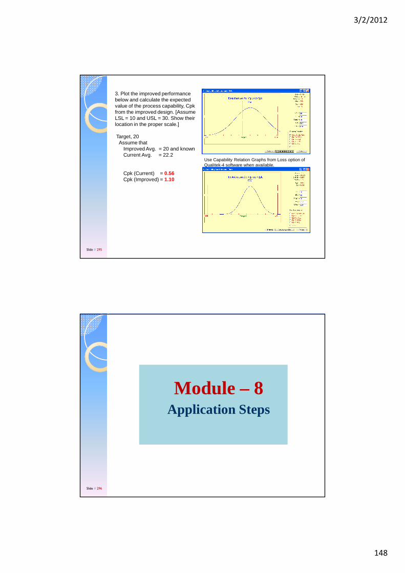
3/2/2012
148
3. Plot the improved performance below and calculate the expected value of the process capability, Cpkfrom the improved design. [Assume LSL = 10 and USL = 30. Show their location in the proper scale.]
Target, 20Assume that
Improved Avg. = 20 and known Current Avg. = 22.2
Cpk (Current) = 0.56Cpk (Improved) = 1.10
Use Capability Relation Graphs from Loss option of Qualitek-4 software when available.
Slide # 295
Module – 8Application Steps
Slide # 296

3/2/2012
149
◦ Can you measure results (Performance)?
◦ Is it possible for you to test (4 -9)?
◦ Do you suspect many factors to influence results?
If answer to above questions is YES, you have much to gain from structured experiments such as a DOE.
Should you do it? (DOE APPLICABILITY TEST)
Slide # 297
Things you should learn from discussions in this module:
HOW TO APPLY
- Planning
- Experiment Design
- Analysis of results
HOW TO PREPARE & PRESENT REPORT (Appendix)
Application Guidelines
Slide # 298

3/2/2012
150
8.1 Description of Application Steps1. Project Selection: Look for a project to apply2. Planning : Arrange for the planning/brainstorming session. 3. Designing : Design experiment & Describe trial conditions.4. Doing : Carry out experiments5. Analyzing: Analyze results6. Confirming: Run confirmation tests
8.2 Brainstorming for Design of Experiments (DOE )Purpose of brainstorming session Who should conduct?Who should host the session?Who should attend?How many should attend?Topics of Discussions
1. Objective of the study (What are you after?)2. Design Factors and their Levels3. Interaction Studies (Which factors are likely to interact?)4. "Noise" Variables (How to create a robust design?)5. Tasks Descriptions and Assignments (Who will do what, how and when?)
Application Guidelines
Ref. Page 8-1
Slide # 299
1. Know how to plan experiments and conduct brainstorming session. Understand basicprinciples of consensus decision making process while working as a team. Know howto:- select criteria and prepare evaluation table- prepare data collection tables- select factors for experiments- decide on the number and values of the levels- compromise on number of factors and interactions- allocate the work assignments for the project (tasks)
2. Know how to design experiments when:- all factors are at the same level (2, 3 or 4 levels)- you wish to study interactions between two 2-level factors- factors are at mixed levels(2, 3 or 4 levels)
3. Can carry out computations for factor average effects and determine:- main effects- optimum condition- performance at the optimum condition
4. Understand the philosophy behind robust design5. 5. Be familiar with the transformation of results to MSD and S/N , and know how to
interpret the conclusions from the analysis.6. Understand the purpose and mechanics of ANOVA calculations:
- interpret the ERROR term & implications of the experimental results - why to pool factors and when to pool them- carry out test for significance and pool factors- calculate confidence interval and what it means
7. Know how to apply the principles of brainstorming problem solving
Application and Analysis Check List
Ref. Page 8-7
Slide # 300
3/2/2012
151
Module - 9Dynamic Systems
Slide # 301
Module - 9Dynamic Systems
Slide # 302
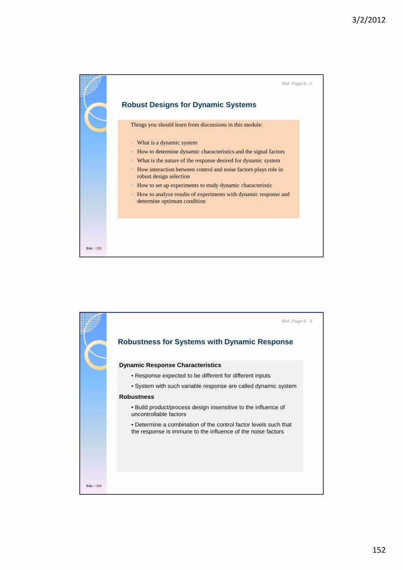
3/2/2012
152
Things you should learn from discussions in this module:
◦ What is a dynamic system
◦ How to determine dynamic characteristics and the signal factors
◦ What is the nature of the response desired for dynamic system
◦ How interaction between control and noise factors plays role in robust design selection
◦ How to set up experiments to study dynamic characteristic
◦ How to analyze results of experiments with dynamic response and determine optimum condition
Robust Designs for Dynamic Systems
Ref. Page 9 - 1
Slide # 303
Robustness for Systems with Dynamic Response
Dynamic Response Characteristics
• Response expected to be different for different inputs
• System with such variable response are called dynamic system
Robustness
• Build product/process design insensitive to the influence of uncontrollable factors
• Determine a combination of the control factor levels such that the response is immune to the influence of the noise factors
Ref. Page 9 - 2
Slide # 304
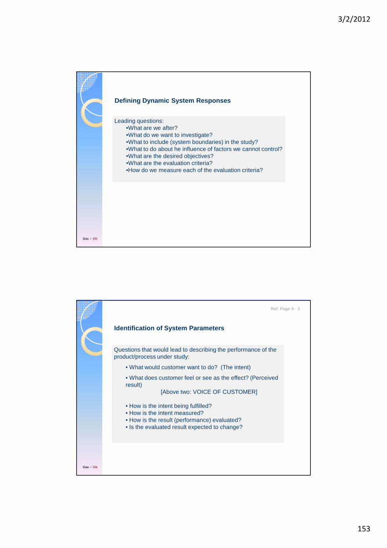
3/2/2012
153
Defining Dynamic System Responses
Leading questions:•What are we after?•What do we want to investigate?•What to include (system boundaries) in the study? •What to do about he influence of factors we cannot control?•What are the desired objectives?•What are the evaluation criteria?•How do we measure each of the evaluation criteria?
Slide # 305
Identification of System Parameters
Questions that would lead to describing the performance of the product/process under study:
• What would customer want to do? (The intent)
• What does customer feel or see as the effect? (Perceived result)
[Above two: VOICE OF CUSTOMER]
• How is the intent being fulfilled?• How is the intent measured?• How is the result (performance) evaluated?• Is the evaluated result expected to change?
Ref. Page 9 - 3
Slide # 306
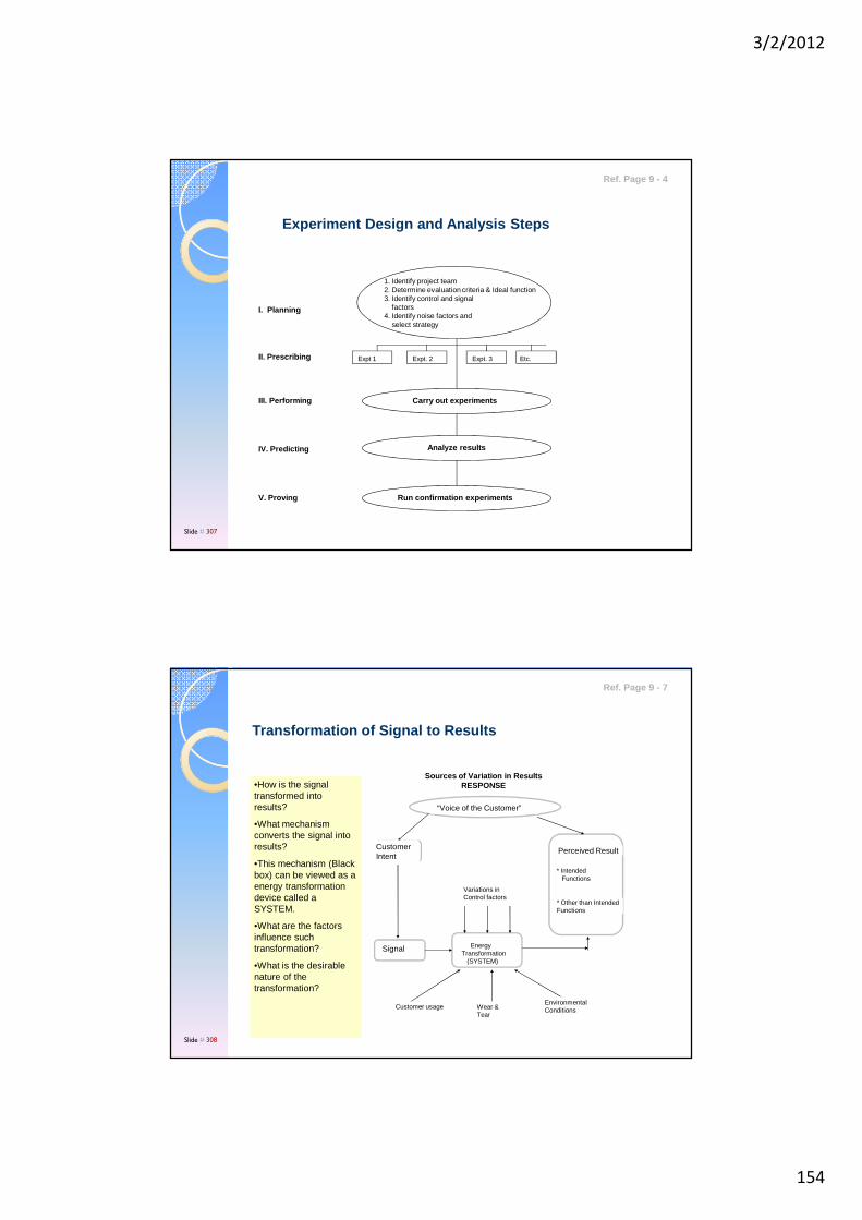
3/2/2012
154
Experiment Design and Analysis Steps
1. Identify project team2. Determine evaluation criteria & Ideal function3. Identify control and signal
factors4. Identify noise factors and
select strategy
Expt 1 Expt. 2 Expt. 3 Etc.
Carry out experiments
Analyze results
Run confirmation experiments
I. Planning
II. Prescribing
III. Performing
IV. Predicting
V. Proving
Ref. Page 9 - 4
Slide # 307
Transformation of Signal to Results
•How is the signal transformed into results?
•What mechanism converts the signal into results?
•This mechanism (Black box) can be viewed as a energy transformation device called a SYSTEM.
•What are the factors influence such transformation?
•What is the desirable nature of the transformation?
“Voice of the Customer”
Customer Intent
Signal
Perceived Result
EnergyTransformation
(SYSTEM)
Sources of Variation in Results RESPONSE
Variations inControl factors
Customer usage Wear & Tear
EnvironmentalConditions
* Intended Functions
* Other than Intended Functions
Ref. Page 9 - 7
Slide # 308
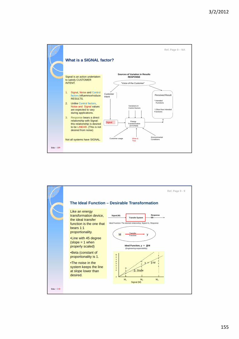
3/2/2012
155
What is a SIGNAL factor?
Signal is an action undertaken to satisfy CUSTOMER INTENT.
1. Signal, Noise and Control factors influemnce/roduceRESULTS.
2. Unlike Control factors, Noise and Signal values are expected to vary during applications.
3. Response bears a direct relationship with Signal: this relationship is desired to be LINEAR. (This is not desired from noise)
Not all systems have SIGNAL.
“Voice of the Customer”
Customer Intent
Signal
Perceived Result
EnergyTransformation
(SYSTEM)
Sources of Variation in Results RESPONSE
Variations inControl factors
Customer usage Wear & Tear
EnvironmentalConditions
* Intended Functions
* Other than Intended Functions
Ref. Page 9 – NA
Slide # 309
The Ideal Function – Desirable Transformation
Like an energy transformation device, the ideal transfer function is the one that bears 1:1 proportionality.
•Line with 45 degree (slope = 1 when properly scaled)
•Beta (constant of proportionality is 1.
•The noise in the system keeps the line at slope lower than desired.
Transfer System
Ideal Function: The desired relationship, Signal Vs. Response
Signal (M) Response (y)
Response
y
M1 M2 M3
Signal (M)
*****
*****
*****
y = β M
β, Slope
M yTransferFunction
Ideal Function, y = ββββ M(Engineering responsibility)
Ref. Page 9 - 9
Slide # 310
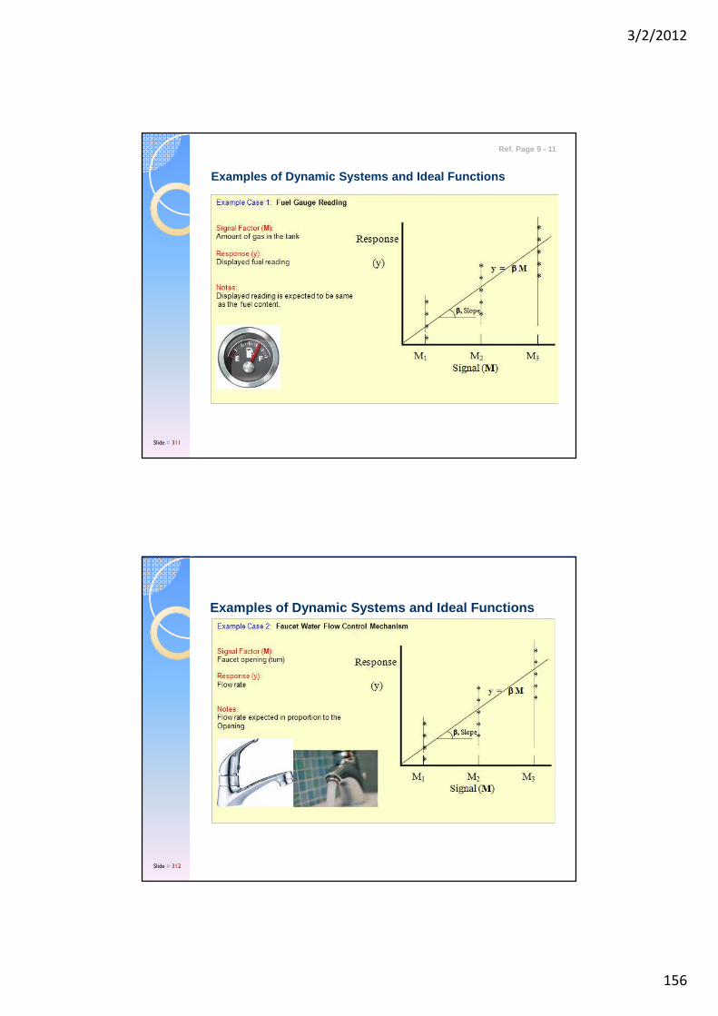
3/2/2012
156
Examples of Dynamic Systems and Ideal Functions
Ref. Page 9 - 11
Slide # 311
Examples of Dynamic Systems and Ideal Functions
Slide # 312
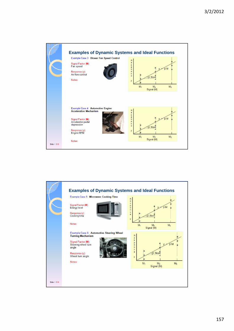
3/2/2012
157
Examples of Dynamic Systems and Ideal Functions
Slide # 313
Examples of Dynamic Systems and Ideal Functions
Slide # 314
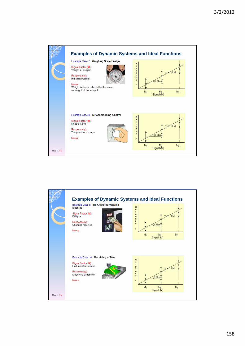
3/2/2012
158
Examples of Dynamic Systems and Ideal Functions
Slide # 315
Examples of Dynamic Systems and Ideal Functions
Slide # 316
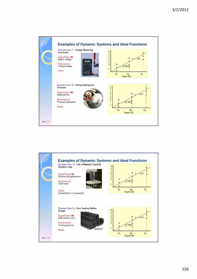
3/2/2012
159
Examples of Dynamic Systems and Ideal Functions
Slide # 317
Examples of Dynamic Systems and Ideal Functions
Slide # 318
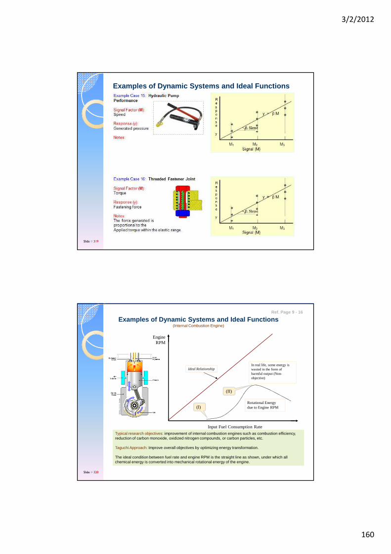
3/2/2012
160
Examples of Dynamic Systems and Ideal Functions
Slide # 319
Examples of Dynamic Systems and Ideal Functions(Internal Combustion Engine)
Typical research objectives: improvement of internal combustion engines such as combustion efficiency, reduction of carbon monoxide, oxidized nitrogen compounds, or carbon particles, etc.
Taguchi Approach: Improve overall objectives by optimizing energy transformation.
The ideal condition between fuel rate and engine RPM is the straight line as shown, under which all chemical energy is converted into mechanical rotational energy of the engine.
Engine RPM
Ideal Relationship
Rotational Energy due to Engine RPM
In real life, some energy is wasted in the form of harmful output (Non-objective)
Input Fuel Consumption Rate
(I)
(II)
Ref. Page 9 - 16
Slide # 320

3/2/2012
161
Examples of Dynamic Systems and Ideal Functions(Internal Combustion Engine)
• In real operating condition, chemical energy of fuel is used to overcome mechanical loss of the engine; thus, the engine RPM is zero if the fuel rate is lower than (I). As fuel rate is increased, RPM slowly increases and reaches its peak value at condition (II). If you keep increasing the fuel rate, however, the RPM may go down, indicating that the increased fuel energy is converted into harmful side effects such as vibration, audible noise, thermal loss in the exhaust pipe, residual fuel, carbon monoxide, nitrogen dioxide, etc.
• When the engine performance and fuel consumption are improved and the harmful side effects are reduced, the real operating condition moves closer to the IDEAL CONDITION which results:
•Reduced deterioration and wear of the engine • Increased reliability & life .
Noise Factors:fuel impurities, temperature distribution variation of the engine, fuel octane values, and lubrication oil viscosity. A good engine is robust against all kinds of noise factors.
(Noise factors are introduced into the experiment by compounding the them into two extreme noise conditions)
Signal (M): Fuel Consumption Rate
Response (Y): Engine RotationDesirable output – Mechanical mobility energy (Y)Unwanted outcome
- Mechanical loss (Vibration, friction, wear, audible noise) - Thermal (Exhaust, radiator,..) - Incomplete combustion reaction (Residual Fuel, Monoxide,
Nitrogen Dioxide, Carbon Particles)
System: Internal Combustion EngineFactors: Fuel, air-fuel mixing, combustion chamber, exhaust system, cylinder-piston design parameters, etc.
The goal of robust design is to minimize the unwanted effects which can be obtained when the performance resembles the ideal function.
Ref. Page 9 - 17
Slide # 321
Other Examples of Dynamic SystemsExample Case 1: Fuel Gauge Reading
Example Case 2: Faucet Water Flow
Example Case 3: Blower Fan Speed Control
Example Case 4: Automotive Engine Acceleration Mechanism
Example Case 5: Microwave Cooking Time
Example Case 6: Automotive Steering Wheel Turning Mechanism
Example Case 7: Weighing Scale Design
Example Case 8: Air-conditioning Control
Example Case 9: Bill Changing Vending
Example Case 10: Machining of Dies
Example Case 11: Voltage Measuring
Example Case 12: Airbag Deployment
Example Case 13: Test of Material Elasticity
Example Case 14: Door Sealing Rubber Design
Example Case 15: Hydraulic Pump Performance
Example Case 16: Threaded Fastener Joint
Example Case 17: Internal Combustion Engine
Ref. Page 9 - NA
Slide # 322

3/2/2012
162
Robustness for Static System – a Model
Static System: Tiger Woods putting golf ballsAugust 11, 2004Top spot : Tiger Woods' hold on the world number one ranking is more tenuous now.
”Vijay Singh has been on Tiger's heels for some time now, and if either Singh, or Ernie Ells were to win the PGA Championship, Woods would relinquish his spot atop the rankings.”
Ref. Page 9 - 18
Slide # 323
Robustness for Dynamic System – a Model
Lance Armstrong rides into Paris, collects record sixth consecutive Tour title (Tour de France)
Sunday July 25, 2004 5:39PM
PARIS (AP) -- Lance Armstrong raced onto the crowd-lined Champs-Elysees as a yellow blur, bathed in the shimmering light of a 24-carat, gold-leaf bike, a golden helmet and the race leader's yellow jersey.
Nutek, Inc. All Rights Reserved Robust Product and Process Designs www.Nutek-us.com Version 0808 Slide # 324
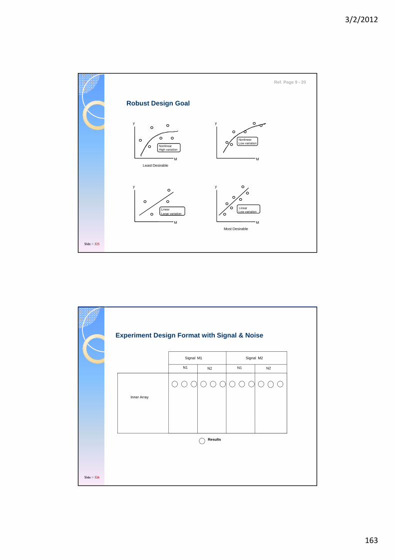
3/2/2012
163
Robust Design Goal
y
M
y
M
y
M
y
M
NonlinearHigh variation
NonlinearLow variation
LinearLarge variation
LinearLow variation
Least Desirable
Most Desirable
Ref. Page 9 - 20
Slide # 325
Experiment Design Format with Signal & Noise Experiment Design Format with Signal & Noise
Inner Array
Signal M1 Signal M2
N1 N2 N1 N2
Results
Slide # 326
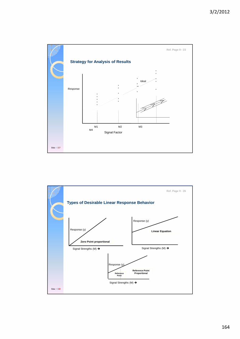
3/2/2012
164
Strategy for Analysis of Results
Ideal
M1 M2 M3M4
Response
*****
**
*
**
*
***
*
**
**
*
Signal Factor
Ref. Page 9 - 23
Slide # 327
Types of Desirable Linear Response Behavior
Response (y)
Zero Point proportional
Signal Strengths (M) �
Response (y)
Linear Equation
Signal Strengths (M) �
Response (y)
Reference PointProportional
Signal Strengths (M) �
Reference Point
Ref. Page 9 - 26
Slide # 328
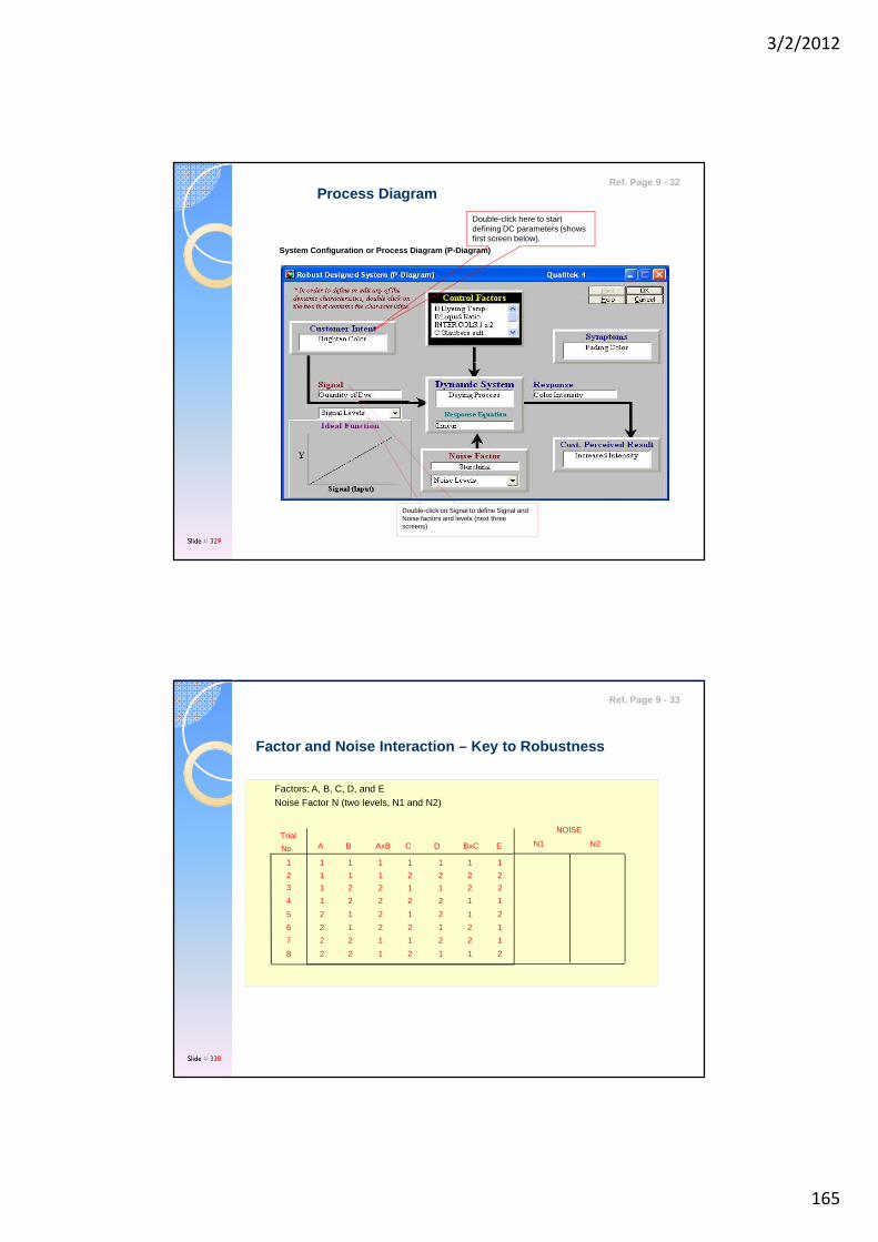
3/2/2012
165
Process Diagram
System Configuration or Process Diagram (P-Diagram)
Double-click here to start defining DC parameters (shows first screen below).
Double-click on Signal to define Signal and Noise factors and levels (next three screens)
Ref. Page 9 - 32
Slide # 329
Factor and Noise Interaction – Key to Robustness
Factors: A, B, C, D, and ENoise Factor N (two levels, N1 and N2)
NOISE
N1 N2
25
11
14
26
7 2
8 2
Trial
No. A
12
3 1
1
1
2
1
2
2
B
1
2
2
1
2
2
1
1
AxB
1
2
C
1
1
2
2
1
2
2
1
E
2
1
1
1
1
2
2
2
1
1
1
2
2
1
2
2
BxC
2
1
2
1
2
1
2
1
D
Ref. Page 9 - 33
Slide # 330
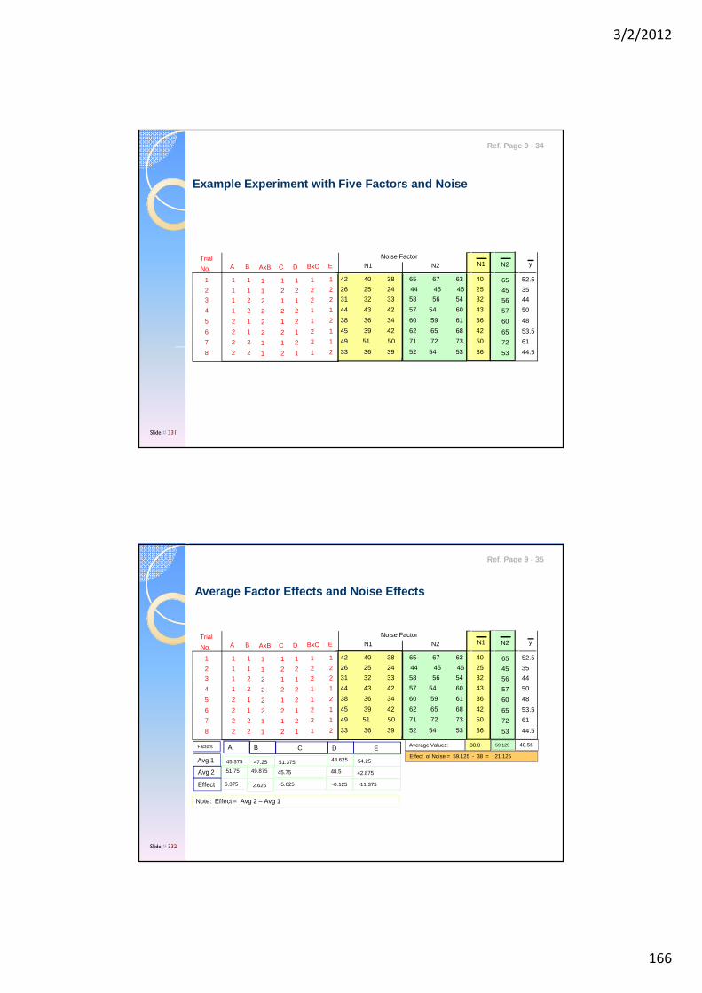
3/2/2012
166
Example Experiment with Five Factors and Noise
38
42
44
45
49
33
26
31
36
40
43
39
51
36
25
32
34
38
42
42
50
39
24
33
65
60
57
62
71
52
44
58
67
59
54
65
72
54
45
56
63
61
60
68
73
53
46
54
N1Noise Factor
N2
5
1
4
6
7
8
Trial
No.
2
3
2
1
1
2
2
2
A
1
1
1
1
2
1
2
2
B
1
2
2
1
2
2
1
1
AxB
1
2
C
1
1
2
2
1
2
2
1
E
2
1
1
1
1
2
2
2
1
1
1
2
2
1
2
2
BxC
2
1
2
1
2
1
2
1
D N1 N2 y
36
40
43
42
50
36
25
32
60
65
57
65
72
53
45
56
48
52.5
50
53.5
61
44.5
35
44
Ref. Page 9 - 34
Slide # 331
Average Factor Effects and Noise Effects
38
42
44
45
49
33
26
31
36
40
43
39
51
36
25
32
34
38
42
42
50
39
24
33
65
60
57
62
71
52
44
58
67
59
54
65
72
54
45
56
63
61
60
68
73
53
46
54
N1Noise Factor
N2
5
1
4
6
7
8
Trial
No.
2
3
2
1
1
2
2
2
A
1
1
1
1
2
1
2
2
B
1
2
2
1
2
2
1
1
AxB
1
2
C
1
1
2
2
1
2
2
1
E
2
1
1
1
1
2
2
2
1
1
1
2
2
1
2
2
BxC
2
1
2
1
2
1
2
1
D N1 N2 y
36
40
43
42
50
36
25
32
60
65
57
65
72
53
45
56
48
52.5
50
53.5
61
44.5
35
44
Effect of Noise = 59.125 - 38 = 21.125
Average Values: 38.0 59.125 48.56A B C D E
45.375 47.25 51.375 48.625 54.25
51.75 49.875 45.75 48.5 42.875
6.375 2.625 -5.625 -0.125 -11.375
Avg 1
Avg 2
Effect
Factors
Note: Effect = Avg 2 – Avg 1
Ref. Page 9 - 35
Slide # 332
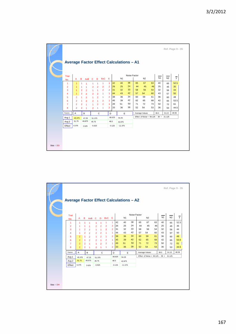
3/2/2012
167
Average Factor Effect Calculations – A1
38
42
44
45
49
33
26
31
36
40
43
39
51
36
25
32
34
38
42
42
50
39
24
33
65
60
57
62
71
52
44
58
67
59
54
65
72
54
45
56
63
61
60
68
73
53
46
54
N1Noise Factor
N2
5
1
4
6
7
8
Trial
No.
2
3
2
1
1
2
2
2
A
1
1
1
1
2
1
2
2
B
1
2
2
1
2
2
1
1
AxB
1
2
C
1
1
2
2
1
2
2
1
E
2
1
1
1
1
2
2
2
1
1
1
2
2
1
2
2
BxC
2
1
2
1
2
1
2
1
D N1 N2 y
36
40
43
42
50
36
25
32
60
65
57
65
72
53
45
56
48
52.5
50
53.5
61
44.5
35
44
Effect of Noise = 59.125 - 38 = 21.125
Average Values: 38.0 59.125 48.56A B C D E
45.375 47.25 51.375 48.625 54.25
51.75 49.875 45.75 48.5 42.875
6.375 2.625 -5.625 -0.125 -11.375
Avg 1
Avg 2
Effect
Factors
Ref. Page 9 - 35
Slide # 333
38
42
44
45
49
33
26
31
36
40
43
39
51
36
25
32
34
38
42
42
50
39
24
33
65
60
57
62
71
52
44
58
67
59
54
65
72
54
45
56
63
61
60
68
73
53
46
54
N1Noise Factor
N2
5
1
4
6
7
8
Trial
No.
2
3
2
1
1
2
2
2
A
1
1
1
1
2
1
2
2
B
1
2
2
1
2
2
1
1
AxB
1
2
C
1
1
2
2
1
2
2
1
E
2
1
1
1
1
2
2
2
1
1
1
2
2
1
2
2
BxC
2
1
2
1
2
1
2
1
D N1 N2 y
36
40
43
42
50
36
25
32
60
65
57
65
72
53
45
56
48
52.5
50
53.5
61
44.5
35
44
Effect of Noise = 59.125 - 38 = 21.125
Average Values: 38.0 59.125 48.56A B C D E
45.375 47.25 51.375 48.625 54.25
51.75 49.875 45.75 48.5 42.875
6.375 2.625 -5.625 -0.125 -11.375
Avg 1
Avg 2
Effect
Factors
Average Factor Effect Calculations – A2
Ref. Page 9 - 35
Slide # 334
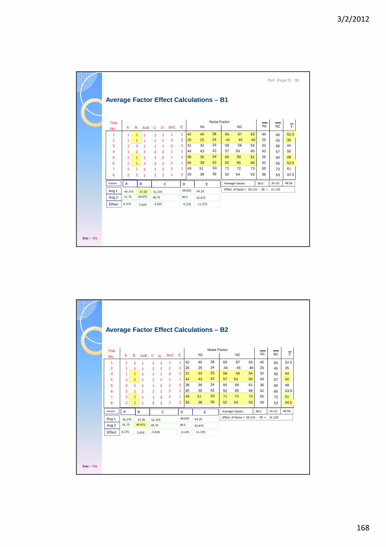
3/2/2012
168
38
42
44
45
49
33
26
31
36
40
43
39
51
36
25
32
34
38
42
42
50
39
24
33
65
60
57
62
71
52
44
58
67
59
54
65
72
54
45
56
63
61
60
68
73
53
46
54
N1Noise Factor
N2
5
1
4
6
7
8
Trial
No.
2
3
2
1
1
2
2
2
A
1
1
1
1
2
1
2
2
B
1
2
2
1
2
2
1
1
AxB
1
2
C
1
1
2
2
1
2
2
1
E
2
1
1
1
1
2
2
2
1
1
1
2
2
1
2
2
BxC
2
1
2
1
2
1
2
1
D N1 N2 y
36
40
43
42
50
36
25
32
60
65
57
65
72
53
45
56
48
52.5
50
53.5
61
44.5
35
44
Effect of Noise = 59.125 - 38 = 21.125
Average Values: 38.0 59.125 48.56A B C D E
45.375 47.25 51.375 48.625 54.25
51.75 49.875 45.75 48.5 42.875
6.375 2.625 -5.625 -0.125 -11.375
Avg 1
Avg 2
Effect
Factors
Average Factor Effect Calculations – B1
Ref. Page 9 - 36
Slide # 335
38
42
44
45
49
33
26
31
36
40
43
39
51
36
25
32
34
38
42
42
50
39
24
33
65
60
57
62
71
52
44
58
67
59
54
65
72
54
45
56
63
61
60
68
73
53
46
54
N1Noise Factor
N2
5
1
4
6
7
8
Trial
No.
2
3
2
1
1
2
2
2
A
1
1
1
1
2
1
2
2
B
1
2
2
1
2
2
1
1
AxB
1
2
C
1
1
2
2
1
2
2
1
E
2
1
1
1
1
2
2
2
1
1
1
2
2
1
2
2
BxC
2
1
2
1
2
1
2
1
DN1 N2 y
36
40
43
42
50
36
25
32
60
65
57
65
72
53
45
56
48
52.5
50
53.5
61
44.5
35
44
Effect of Noise = 59.125 - 38 = 21.125
Average Values: 38.0 59.125 48.56A B C D E
45.375 47.25 51.375 48.625 54.25
51.75 49.875 45.75 48.5 42.875
6.375 2.625 -5.625 -0.125 -11.375
Avg 1
Avg 2
Effect
Factors
Average Factor Effect Calculations – B2
Slide # 336
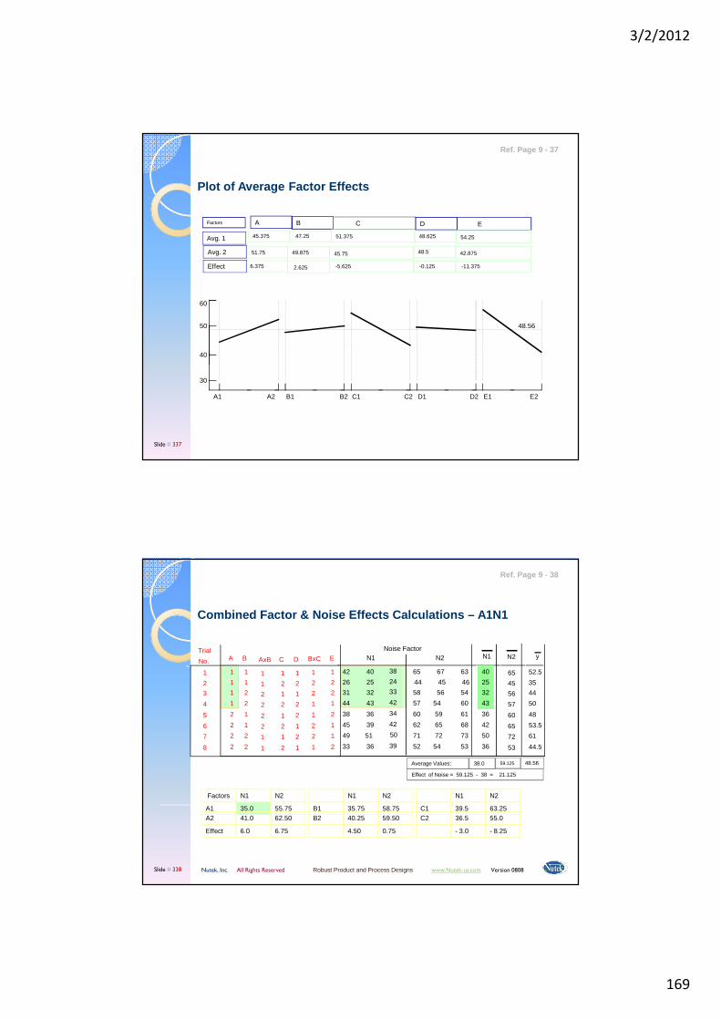
3/2/2012
169
A B C D E
45.375 47.25 51.375 48.625 54.25
51.75 49.875 45.75 48.5 42.875
6.375 2.625 -5.625 -0.125 -11.375
Avg. 1
Avg. 2
Effect
Factors
60
40
50
30
48.56
A1 A2 B1 B2 C1 C2 D1 D2 E1 E2
Plot of Average Factor Effects
Ref. Page 9 - 37
Slide # 337
N1
35.041.0
6.0
N2
55.7562.50
6.75
Factors
A1A2
Effect
N1
35.7540.25
4.50
N2
58.7559.50
0.75
B1B2
N1
39.536.5
- 3.0
N2
63.2555.0
- 8.25
C1C2
38
42
44
45
49
33
26
31
36
40
43
39
51
36
25
32
34
38
42
42
50
39
24
33
65
60
57
62
71
52
44
58
67
59
54
65
72
54
45
56
63
61
60
68
73
53
46
54
N1Noise Factor
N2
5
1
4
6
7
8
Trial
No.
2
3
2
1
1
2
2
2
A
1
1
1
1
2
1
2
2
B
1
2
2
1
2
2
1
1
AxB
1
2
C
1
1
2
2
1
2
2
1
E
2
1
1
1
1
2
2
2
1
1
1
2
2
1
2
2
BxC
2
1
2
1
2
1
2
1
D N1 N2 y
36
40
43
42
50
36
25
32
60
65
57
65
72
53
45
56
48
52.5
50
53.5
61
44.5
35
44
Effect of Noise = 59.125 - 38 = 21.125
Average Values: 38.0 59.125 48.56
Combined Factor & Noise Effects Calculations – A1N1
Nutek, Inc. All Rights Reserved Robust Product and Process Designs www.Nutek-us.com Version 0808 Slide # 338
Ref. Page 9 - 38
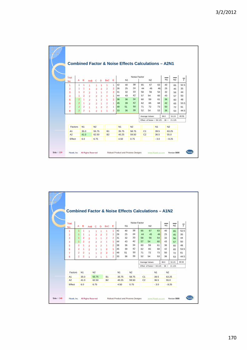
3/2/2012
170
N1
35.0
41.0
6.0
N2
55.75
62.50
6.75
Factors
A1
A2
Effect
N1
35.75
40.25
4.50
N2
58.75
59.50
0.75
B1
B2
N1
39.5
36.5
- 3.0
N2
63.25
55.0
- 8.25
C1
C2
38
42
44
45
49
33
26
31
36
40
43
39
51
36
25
32
34
38
42
42
50
39
24
33
65
60
57
62
71
52
44
58
67
59
54
65
72
54
45
56
63
61
60
68
73
53
46
54
N1Noise Factor
N2
5
1
4
6
7
8
Trial
No.
2
3
2
1
1
2
2
2
A
1
1
1
1
2
1
2
2
B
1
2
2
1
2
2
1
1
AxB
1
2
C
1
1
2
2
1
2
2
1
E
2
1
1
1
1
2
2
2
1
1
1
2
2
1
2
2
BxC
2
1
2
1
2
1
2
1
D N1 N2 y
36
40
43
42
50
36
25
32
60
65
57
65
72
53
45
56
48
52.5
50
53.5
61
44.5
35
44
Effect of Noise = 59.125 - 38 = 21.125
Average Values: 38.0 59.125 48.56
Combined Factor & Noise Effects Calculations – A2N1
Nutek, Inc. All Rights Reserved Robust Product and Process Designs www.Nutek-us.com Version 0808 Slide # 339
N1
35.041.0
6.0
N2
55.7562.50
6.75
Factors
A1A2
Effect
N1
35.7540.25
4.50
N2
58.7559.50
0.75
B1B2
N1
39.536.5
- 3.0
N2
63.2555.0
- 8.25
C1C2
38
42
44
45
49
33
26
31
36
40
43
39
51
36
25
32
34
38
42
42
50
39
24
33
65
60
57
62
71
52
44
58
67
59
54
65
72
54
45
56
63
61
60
68
73
53
46
54
N1Noise Factor
N2
5
1
4
6
7
8
Trial
No.
2
3
2
1
1
2
2
2
A
1
1
1
1
2
1
2
2
B
1
2
2
1
2
2
1
1
AxB
1
2
C
1
1
2
2
1
2
2
1
E
2
1
1
1
1
2
2
2
1
1
1
2
2
1
2
2
BxC
2
1
2
1
2
1
2
1
D N1 N2 y
36
40
43
42
50
36
25
32
60
65
57
65
72
53
45
56
48
52.5
50
53.5
61
44.5
35
44
Effect of Noise = 59.125 - 38 = 21.125
Average Values: 38.0 59.125 48.56
Combined Factor & Noise Effects Calculations – A1N2
Nutek, Inc. All Rights Reserved Robust Product and Process Designs www.Nutek-us.com Version 0808 Slide # 340
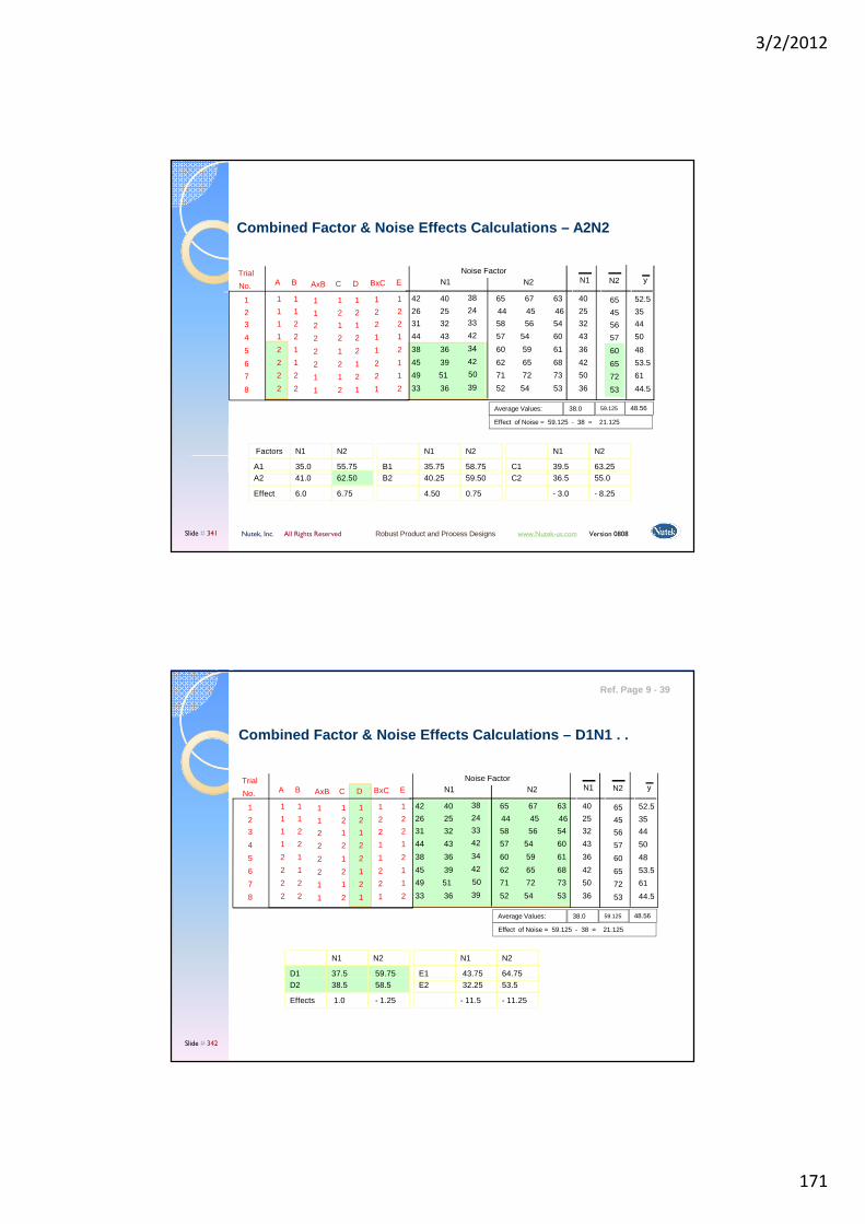
3/2/2012
171
N1
35.041.0
6.0
N2
55.7562.50
6.75
Factors
A1A2
Effect
N1
35.7540.25
4.50
N2
58.7559.50
0.75
B1B2
N1
39.536.5
- 3.0
N2
63.2555.0
- 8.25
C1C2
38
42
44
45
49
33
26
31
36
40
43
39
51
36
25
32
34
38
42
42
50
39
24
33
65
60
57
62
71
52
44
58
67
59
54
65
72
54
45
56
63
61
60
68
73
53
46
54
N1Noise Factor
N2
5
1
4
6
7
8
Trial
No.
2
3
2
1
1
2
2
2
A
1
1
1
1
2
1
2
2
B
1
2
2
1
2
2
1
1
AxB
1
2
C
1
1
2
2
1
2
2
1
E
2
1
1
1
1
2
2
2
1
1
1
2
2
1
2
2
BxC
2
1
2
1
2
1
2
1
D N1 N2 y
36
40
43
42
50
36
25
32
60
65
57
65
72
53
45
56
48
52.5
50
53.5
61
44.5
35
44
Effect of Noise = 59.125 - 38 = 21.125
Average Values: 38.0 59.125 48.56
Combined Factor & Noise Effects Calculations – A2N2
Nutek, Inc. All Rights Reserved Robust Product and Process Designs www.Nutek-us.com Version 0808 Slide # 341
N1
37.5 38.5
1.0
N2
59.7558.5
- 1.25
D1D2
Effects
N1
43.75 32.25
- 11.5
N2
64.75 53.5
- 11.25
E1E2
38
42
44
45
49
33
26
31
36
40
43
39
51
36
25
32
34
38
42
42
50
39
24
33
65
60
57
62
71
52
44
58
67
59
54
65
72
54
45
56
63
61
60
68
73
53
46
54
N1Noise Factor
N2
5
1
4
6
7
8
Trial
No.
2
3
2
1
1
2
2
2
A
1
1
1
1
2
1
2
2
B
1
2
2
1
2
2
1
1
AxB
1
2
C
1
1
2
2
1
2
2
1
E
2
1
1
1
1
2
2
2
1
1
1
2
2
1
2
2
BxC
2
1
2
1
2
1
2
1
D N1 N2 y
36
40
43
42
50
36
25
32
60
65
57
65
72
53
45
56
48
52.5
50
53.5
61
44.5
35
44
Effect of Noise = 59.125 - 38 = 21.125
Average Values: 38.0 59.125 48.56
Combined Factor & Noise Effects Calculations – D1N1 . .
Ref. Page 9 - 39
Slide # 342
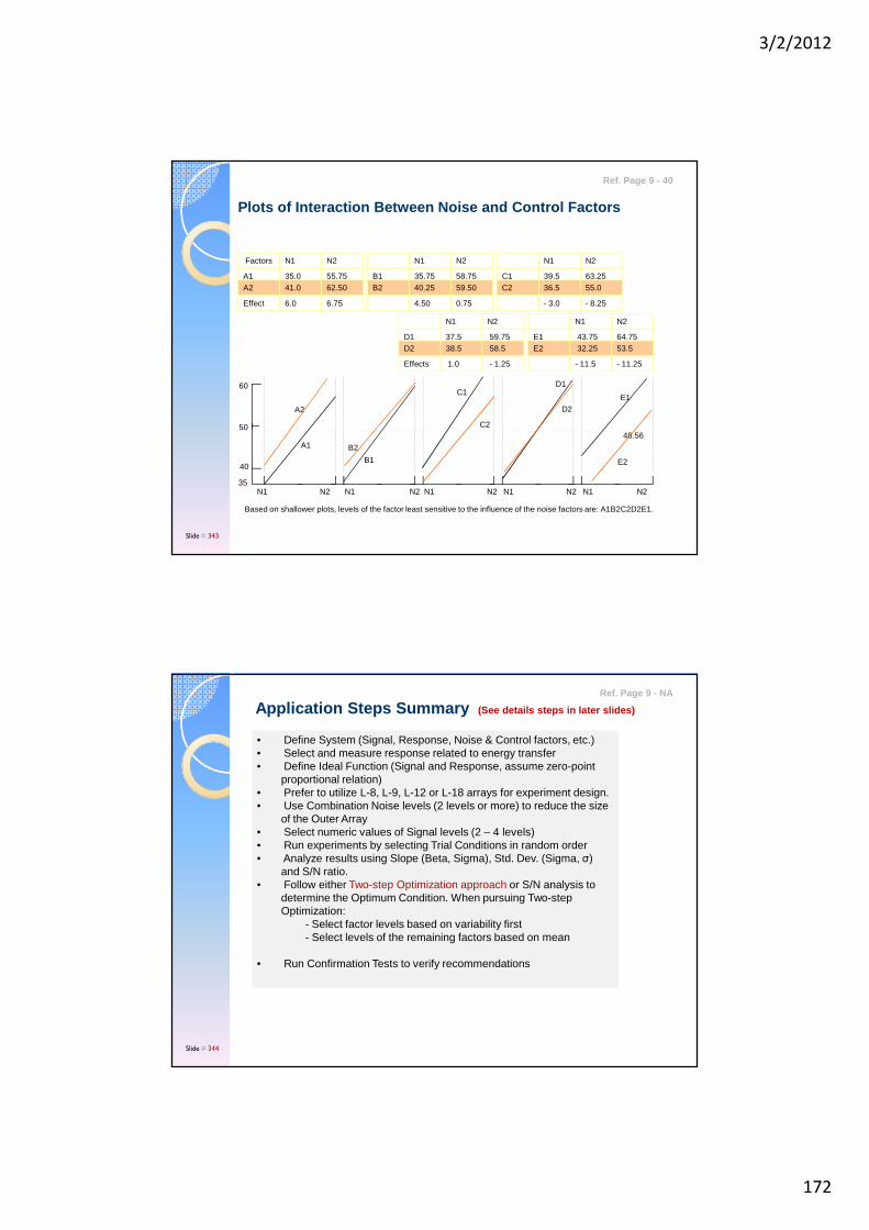
3/2/2012
172
Plots of Interaction Between Noise and Control Fact ors
N1
37.5 38.5
1.0
N2
59.7558.5
- 1.25
D1D2
Effects
N1
43.75 32.25
- 11.5
N2
64.75 53.5
- 11.25
E1E2
N1
35.041.0
6.0
N2
55.7562.50
6.75
Factors
A1A2
Effect
N1
35.7540.25
4.50
N2
58.7559.50
0.75
B1B2
N1
39.536.5
- 3.0
N2
63.2555.0
- 8.25
C1C2
48.56
N1 N2 N1 N2 N1 N2 N1 N2 N1 N2
60
40
50
35
A1
A2
B2
C2
D2
E2B1
D1
E1C1
Based on shallower plots, levels of the factor least sensitive to the influence of the noise factors are: A1B2C2D2E1.
Ref. Page 9 - 40
Slide # 343
Application Steps Summary (See details steps in later slides)
• Define System (Signal, Response, Noise & Control factors, etc.)• Select and measure response related to energy transfer• Define Ideal Function (Signal and Response, assume zero-point
proportional relation) • Prefer to utilize L-8, L-9, L-12 or L-18 arrays for experiment design.• Use Combination Noise levels (2 levels or more) to reduce the size
of the Outer Array• Select numeric values of Signal levels (2 – 4 levels)• Run experiments by selecting Trial Conditions in random order• Analyze results using Slope (Beta, Sigma), Std. Dev. (Sigma, σ)
and S/N ratio.• Follow either Two-step Optimization approach or S/N analysis to
determine the Optimum Condition. When pursuing Two-step Optimization:
- Select factor levels based on variability first- Select levels of the remaining factors based on mean
• Run Confirmation Tests to verify recommendations
Ref. Page 9 - NA
Slide # 344
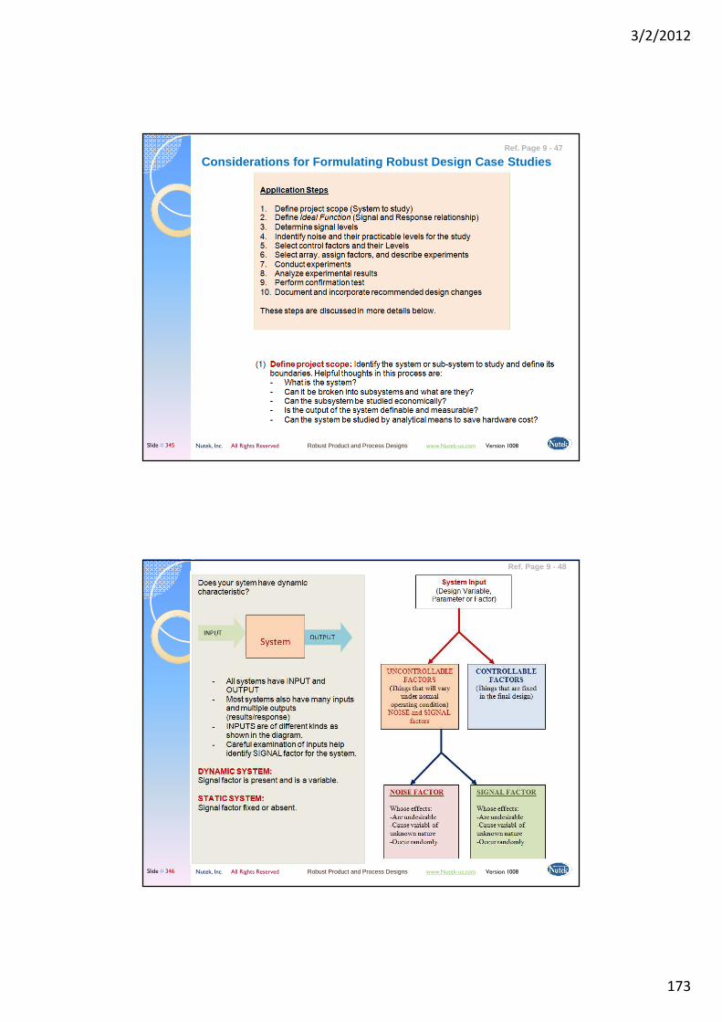
3/2/2012
173
Nutek, Inc. All Rights Reserved Robust Product and Process Designs www.Nutek-us.com Version 1008 Slide # 345
Considerations for Formulating Robust Design Case S tudiesRef. Page 9 - 47
Nutek, Inc. All Rights Reserved Robust Product and Process Designs www.Nutek-us.com Version 1008 Slide # 346
Ref. Page 9 - 48
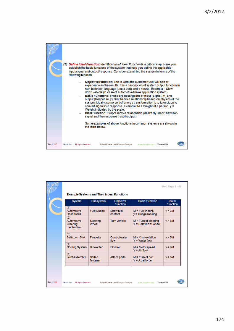
3/2/2012
174
Nutek, Inc. All Rights Reserved Robust Product and Process Designs www.Nutek-us.com Version 1008 Slide # 347
Nutek, Inc. All Rights Reserved Robust Product and Process Designs www.Nutek-us.com Version 1008 Slide # 348
Ref. Page 9 - 49

3/2/2012
175
Nutek, Inc. All Rights Reserved Robust Product and Process Designs www.Nutek-us.com Version 1008 Slide # 349
Ref. Page 9 - 49
Nutek, Inc. All Rights Reserved Robust Product and Process Designs www.Nutek-us.com Version 1008 Slide # 350
………….
Ref. Page 9 - 51
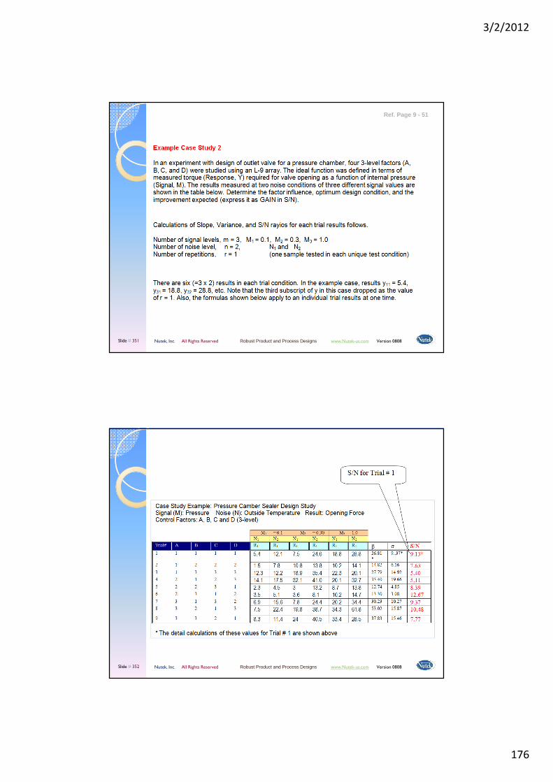
3/2/2012
176
Nutek, Inc. All Rights Reserved Robust Product and Process Designs www.Nutek-us.com Version 0808 Slide # 351
Ref. Page 9 - 51
Nutek, Inc. All Rights Reserved Robust Product and Process Designs www.Nutek-us.com Version 0808 Slide # 352

3/2/2012
177
Nutek, Inc. All Rights Reserved Robust Product and Process Designs www.Nutek-us.com Version 0808 Slide # 353
Computation of Slope (Beta)
( 0.12 + 0.12 ) + ( 0.32 + 0.32 ) + ( 1.02 + 1.02 )
(0.1 x 5.4 + 0.1 x 12.1) + (0.3 x 7.5 + 0.3 x 24.6) + (1.0 x 18.8 + 1.0 x 28.8) β =
= [ 1.75 + 9.63 + 47.6 ] / 2.20 or β = 26.809
Number of signal levels, m = 3, M1 = 0.1, M2 = 0.3, M3 = 1.0Number of noise level, n = 2, N1 and N2 Number of repetitions, r = 1 (one sample tested in each unique test condition)
Ref. Page 9 - 51
Nutek, Inc. All Rights Reserved Robust Product and Process Designs www.Nutek-us.com Version 0808 Slide # 354
Variance (Sigma 2) CalculationRef. Page 9 - 52
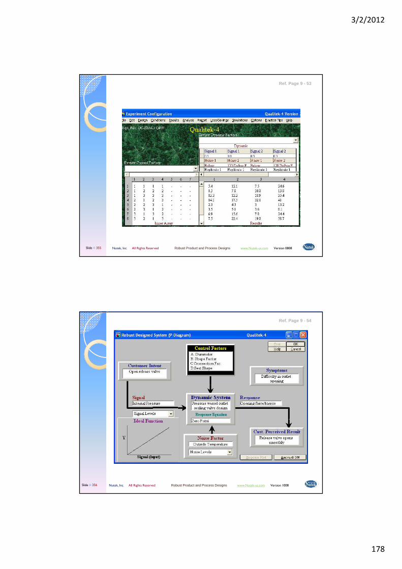
3/2/2012
178
Nutek, Inc. All Rights Reserved Robust Product and Process Designs www.Nutek-us.com Version 0808 Slide # 355
Ref. Page 9 - 53
Nutek, Inc. All Rights Reserved Robust Product and Process Designs www.Nutek-us.com Version 1008 Slide # 356
Ref. Page 9 - 54
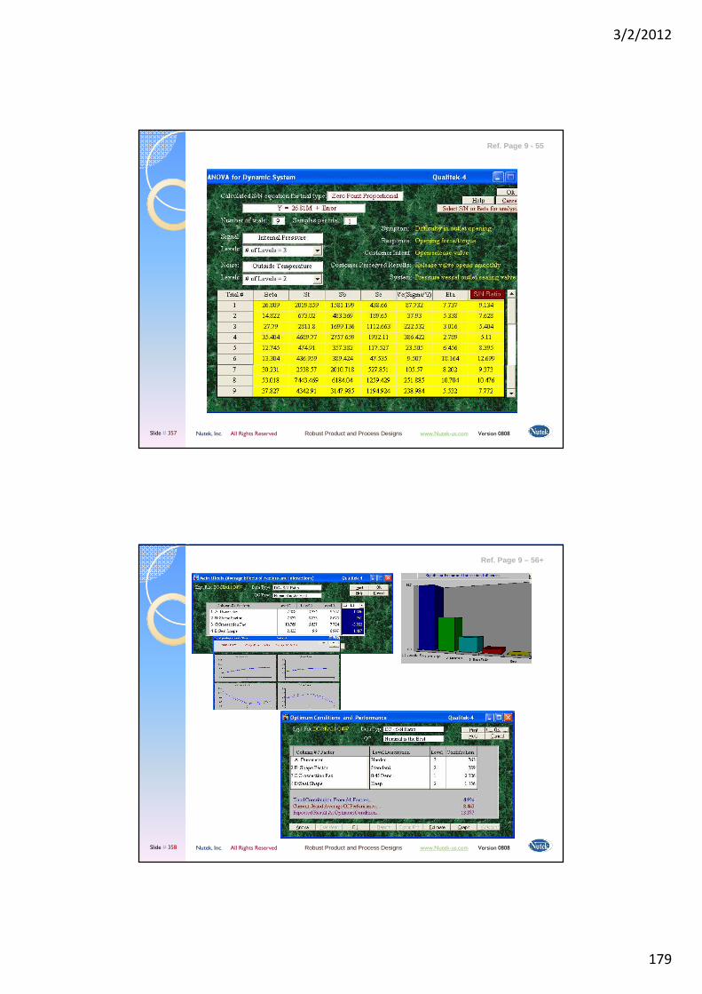
3/2/2012
179
Nutek, Inc. All Rights Reserved Robust Product and Process Designs www.Nutek-us.com Version 0808 Slide # 357
Ref. Page 9 - 55
Nutek, Inc. All Rights Reserved Robust Product and Process Designs www.Nutek-us.com Version 0808 Slide # 358
Ref. Page 9 – 56+

3/2/2012
180
Nutek, Inc. All Rights Reserved Robust Product and Process Designs www.Nutek-us.com Version 0808 Slide # 359
Design Improvement (GAIN)
Expected Gain: 13.377 – 8.443 = 4.934 (dB or S/N)
Ref. Page 9 - 57
Nutek, Inc. All Rights Reserved Robust Product and Process Designs www.Nutek-us.com Version 0808 Slide # 360
Helicopter Fabrication Note: Use a small scissors to make 4 cuts along the dotted lines on the desired paper stock. Fold WINGS and LOWER BODY uniformly.
Ref. Page 9 - 57

3/2/2012
181
Nutek, Inc. All Rights Reserved Robust Product and Process Designs www.Nutek-us.com Version 0808 Slide # 361
Taguchi's Quality Engineering Handbook - Genichi Taguchi, Subir Chowdhury, Yuin Wu, ISBN: 978-0-471-41334-9, Hardcover,1696 page.
Popular Reference for Case Studies with Dynamic Characteristic
Ref. Page 9 - 58
Nutek, Inc. All Rights Reserved Robust Product and Process Designs www.Nutek-us.com Version 0808 Slide # 362
Ref. Page 9 - 60

3/2/2012
182
Nutek, Inc. All Rights Reserved Robust Product and Process Designs www.Nutek-us.com Version 0808 Slide # 363
Ref. Page 9 - 60
Nutek, Inc. All Rights Reserved Robust Product and Process Designs www.Nutek-us.com Version 0808 Slide # 364
Special TopicSpecial TopicQualitekQualitek--4 4
Automatic Design and Analysis of Taguchi ExperimentsAutomatic Design and Analysis of Taguchi Experiments
3/2/2012
183
QualitekQualitek--44Automatic Design and Analysis of Taguchi experimentsAutomatic Design and Analysis of Taguchi experiments
Slide # 365
Getting Started withGetting Started with
QualitekQualitek--4 (QT4)4 (QT4)A A quick tour of the software capabilitiesquick tour of the software capabilities
In case you have not yet downloaded and installed the software in your computer, please do so by visiting www.nutek-us.com/wp-dm4.html or by pasting this link as URL (http://nutek-us.com/q4wxpdemo.zip ) and directly download files from our site.
Slide # 366

3/2/2012
184
What What does Qualitekdoes Qualitek--4 do?4 do?
� Designs Taguchi Experiments
Automatically: QT4 can design simple of mixed level experiments when you only describe the factors and levels.
Manually: QT4 allows you to select the array and assign factors to the columns as you want. Unused columns and Triangular Table information is made readily available on demand.
� Analyzes results with a few Clicks of Mouse
Normally you would start with DESIGN of your experiment using Qualitek-4. Since, we already have an example, PISTON.Q4W, experiment designed, let us first see how Qualitek-4 can ANALYZEresults. Later, we will see how Qualitek-4 capabilities helps us DESIGNour own experiments.
Slide # 367
Let’s Get Started Let’s Get Started --11(Install software and explore some capabilities)(Install software and explore some capabilities)
Run Qualitek-4 (QT4)program from your computer and click OK past the Registration Screen to the experiment configuration screen.
Notice that experiment file PISTON.Q4W is already loaded in memory. If not, OPEN file PISTON.Q4W from FILE menu.
Slide # 368

3/2/2012
185
Nutek, Inc. All Rights Reserved Robust Product and Process Designs www.Nutek-us.com Version 0808 Slide # 369
Practice Session with QualitekPractice Session with Qualitek--44Ref. Page A-21
Nutek, Inc. All Rights Reserved Robust Product and Process Designs www.Nutek-us.com Version 0808 Slide # 370
Ref. Page A-21
Practice Session with QualitekPractice Session with Qualitek--44(Refer to Page 21 of APPENDIX for more detail guide)(Refer to Page 21 of APPENDIX for more detail guide)

3/2/2012
186
Nutek, Inc. All Rights Reserved Robust Product and Process Designs www.Nutek-us.com Version 0808 Slide # 371
Special TopicSpecial TopicAnalytical StudyAnalytical Study
Nutek, Inc. All Rights Reserved Robust Product and Process Designs www.Nutek-us.com Version 0808 Slide # 372
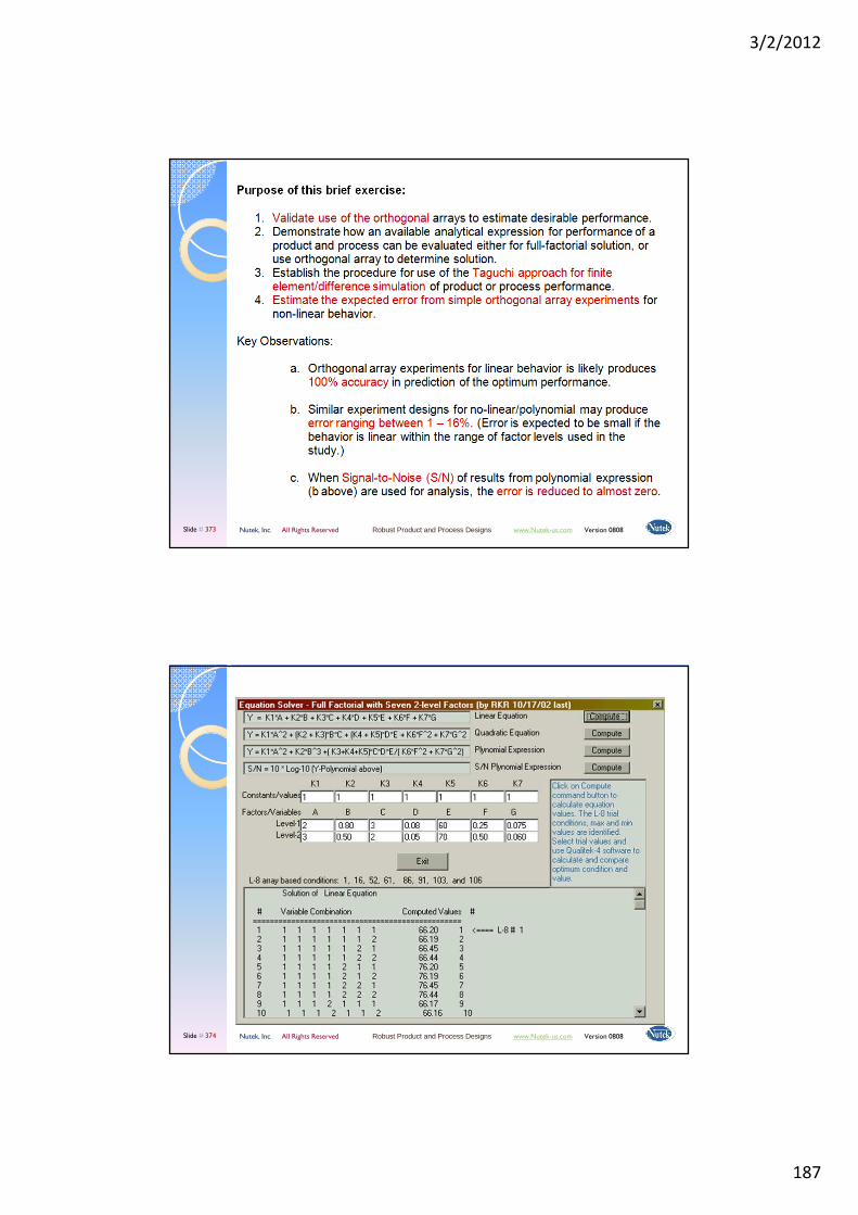
3/2/2012
187
Nutek, Inc. All Rights Reserved Robust Product and Process Designs www.Nutek-us.com Version 0808 Slide # 373
Nutek, Inc. All Rights Reserved Robust Product and Process Designs www.Nutek-us.com Version 0808 Slide # 374
xx
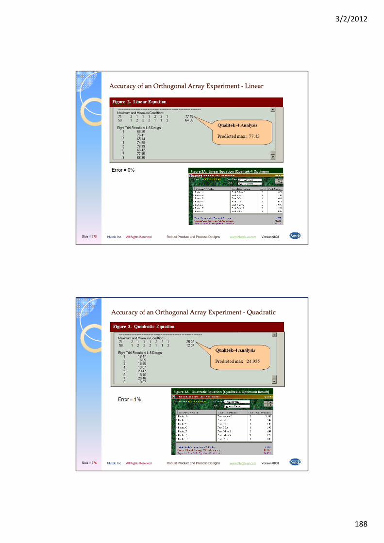
3/2/2012
188
Nutek, Inc. All Rights Reserved Robust Product and Process Designs www.Nutek-us.com Version 0808 Slide # 375
Accuracy of an Orthogonal Array Experiment Accuracy of an Orthogonal Array Experiment -- LinearLinear
Figure 2A. Linear Equation (Qualitek-4 Optimum
Result)
Nutek, Inc. All Rights Reserved Robust Product and Process Designs www.Nutek-us.com Version 0808 Slide # 376
Accuracy of an Orthogonal Array Experiment Accuracy of an Orthogonal Array Experiment -- QuadraticQuadratic
Figure 3A. Quatratic Equation (Qualitek-4 Optimum Result)
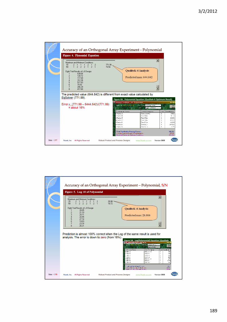
3/2/2012
189
Nutek, Inc. All Rights Reserved Robust Product and Process Designs www.Nutek-us.com Version 0808 Slide # 377
Accuracy of an Orthogonal Array Experiment Accuracy of an Orthogonal Array Experiment -- PolynomialPolynomial
Figure 4A. Polynomial Equation (Qualitek-4 Optimum Result)
Nutek, Inc. All Rights Reserved Robust Product and Process Designs www.Nutek-us.com Version 0808 Slide # 378
Accuracy of an Orthogonal Array Experiment Accuracy of an Orthogonal Array Experiment –– Polynomial, Polynomial, S/NS/N
Figure 5A. Log(Polynomial) Equation (Qualitek-
4 Optimum Result)
3/2/2012
190
Appendix-References
Slide # 379
Ref. Page A-1
Slide # 380
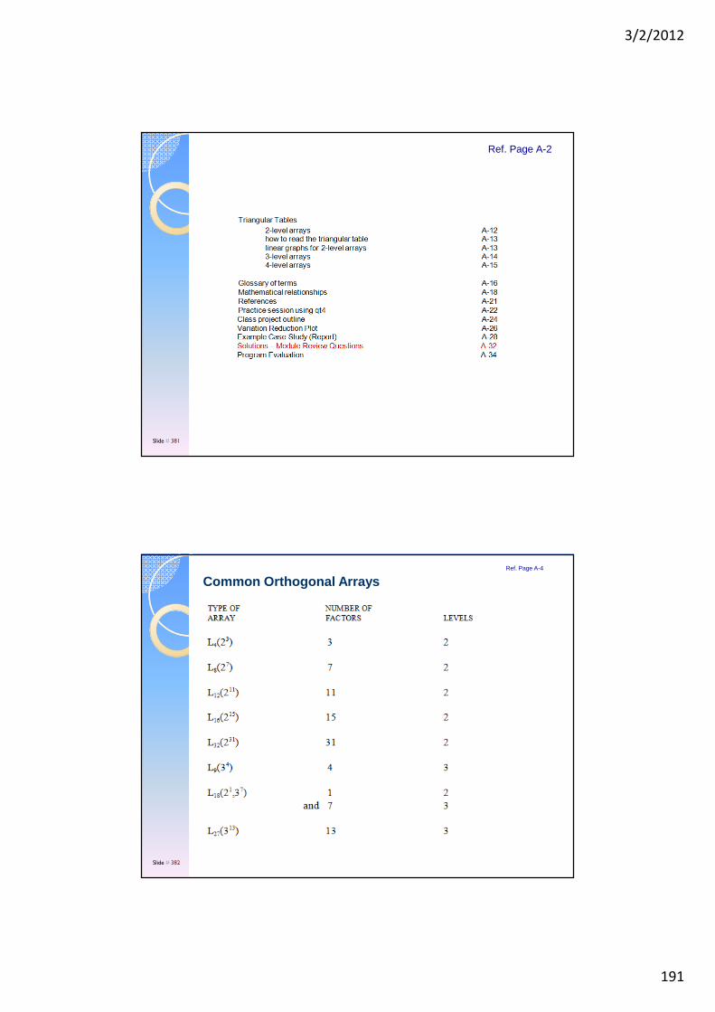
3/2/2012
191
Ref. Page A-2
Slide # 381
Common Orthogonal ArraysRef. Page A-4
Slide # 382
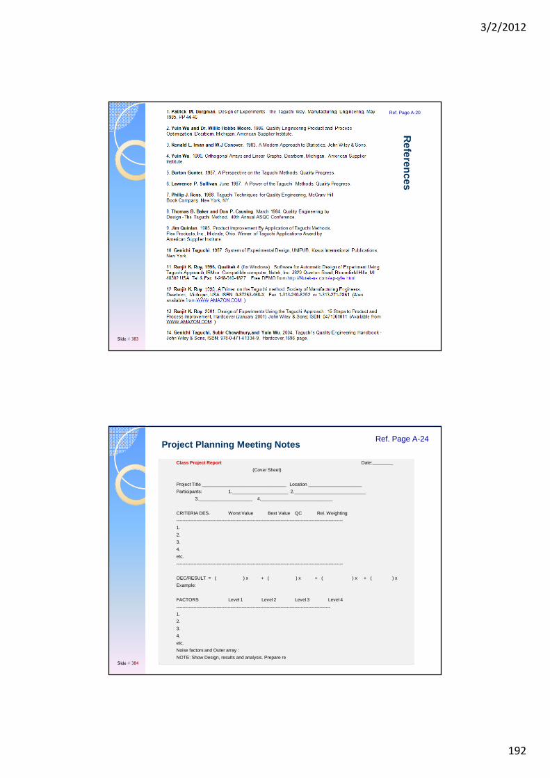
3/2/2012
192
References
Ref. Page A-20
Slide # 383
Class Project Report Date:________
(Cover Sheet)
Project Title _________________________________ Location _____________________
Participants: 1.______________________ 2.____________________________
3._____________________ 4.____________________________
CRITERIA DES. Worst Value Best Value QC Rel. Weighting
-----------------------------------------------------------------------------------------------------------
1.
2.
3.
4.
etc.
-----------------------------------------------------------------------------------------------------------
OEC/RESULT = ( ) x + ( ) x + ( ) x + ( ) x
Example:
FACTORS Level 1 Level 2 Level 3 Level 4
---------------------------------------------------------------------------------------------------
1.
2.
3.
4.
etc.
Noise factors and Outer array :
NOTE: Show Design, results and analysis. Prepare re
Project Planning Meeting NotesRef. Page A-24
Slide # 384
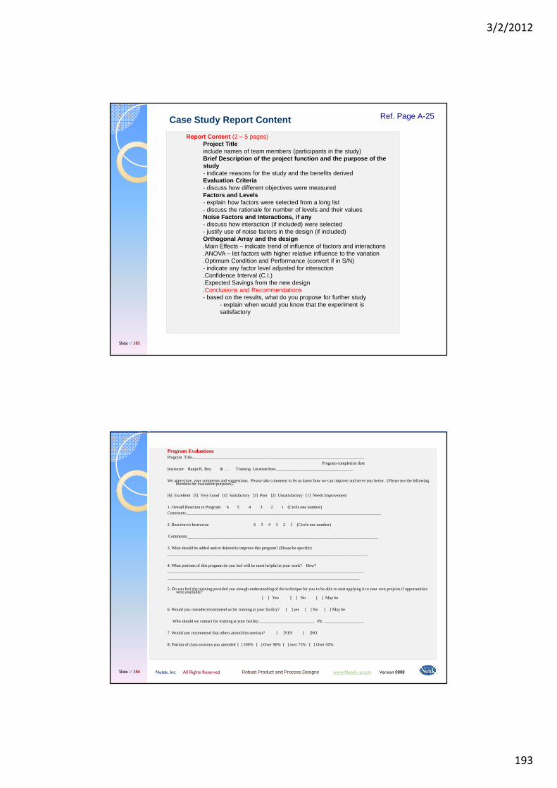
3/2/2012
193
Case Study Report Content
Report Content (2 – 5 pages)Project Titleinclude names of team members (participants in the study)Brief Description of the project function and the p urpose of the study- indicate reasons for the study and the benefits derivedEvaluation Criteria- discuss how different objectives were measuredFactors and Levels- explain how factors were selected from a long list - discuss the rationale for number of levels and their valuesNoise Factors and Interactions, if any- discuss how interaction (if included) were selected- justify use of noise factors in the design (if included)Orthogonal Array and the design.Main Effects – indicate trend of influence of factors and interactions.ANOVA – list factors with higher relative influence to the variation .Optimum Condition and Performance (convert if in S/N) - indicate any factor level adjusted for interaction .Confidence Interval (C.I.).Expected Savings from the new design.Conclusions and Recommendations- based on the results, what do you propose for further study
- explain when would you know that the experiment is satisfactory
Ref. Page A-25
Slide # 385
Program EvaluationsProgram EvaluationsProgram Title_____________________________________ ____________________________________________
Program completion dateInstructor Ranjit K. Roy & …. Training Location/host.____________________________________
We appreciate your comments and suggestions. Please take a moment to let us know how we can improve and serve you better. (Please use the following numbers for evaluation purposes).
[6] Excellent [5] Very Good [4] Satisfactory [3] Poor [2] Unsatisfactory [1] Needs Improvement
1. Overall Reaction to Program: 6 5 4 3 2 1 (Circle one number)Comments:____________________________________________________________________________________________
2. Reaction to Instructor: 6 5 4 3 2 1 (Circle one number)
Comments:__________________________________________________________________________________________
3. What should be added and/or deleted to improve this program? (Please be specific)_______________________________________________________________________________________________
4. What portions of this program do you feel will be most helpful at your work? How?________________________________________________________________________________________________________________________________________________________________________________________
5. Do you feel the training provided you enough understanding of the technique for you to be able to start applying it to your own projects if opportunities were available?
[ ] Yes [ ] No [ ] May be
6. Would you consider/recommend us for training at your facility? [ ] yes [ ] No [ ] May be
Who should we contact for training at your facility __________________________ Ph: ___________________
7. Would you recommend that others attend this seminar? [ ]YES [ ]NO
8. Portion of class sessions you attended [ ] 100% [ ] Over 90% [ ] over 75% [ ] Over 50%
Nutek, Inc. All Rights Reserved Robust Product and Process Designs www.Nutek-us.com Version 0808 Slide # 386

3/2/2012
194
Taguchi Experimental Design TechniquesTaguchi Experimental Design Techniques
OUR SERVICES
� Training & Workshop
� Problem Solving and Assistance with application
� Text Books
� Software (Free DEMO download)
Nutek, Inc.3 829 Quarton Road, Bloomfield Hills, MI 48302.
[email protected] www.Nutek-us.com
Slide # 387


![Report on a Future NEO physical properties database · ”, in proc. IAA Planetary Defense Conference, 2011. [RD12] Di Pippo S. and Perozzi E. European Operational Initiative on NEO](https://img.pdfslide.us/doc/110x75/5ed392f96b0f3821083892c7/report-on-a-future-neo-physical-properties-database-a-in-proc-iaa-planetary.jpg)


![Action in Support of the Federal Authority’s Strategic ...Miruna, Dobre Hugo, Piree Jacques, Nicolas Belgian Science Policy ... Ludger Koenders Wiley-VCH Veerlag GmbH 2005 [RD12]](https://img.pdfslide.us/doc/110x75/5ac056f37f8b9ae45b8c0aff/action-in-support-of-the-federal-authoritys-strategic-miruna-dobre-hugo.jpg)