arX

iv:a

stro

-ph/

0303

521v

1 2

4 M

ar 2

003

Gasoline: An adaptable implementation of

TreeSPH

J.W. Wadsley a J. Stadel b T. Quinn c

aDepartment of Physics and Astronomy, McMaster University, Hamilton,

Canada 1

bInstitute for Theoretical Physics, University of Zurich, Switzerland

cAstronomy Department, University of Washington, Seattle, Washington, USA

Abstract

The key algorithms and features of the Gasoline code for parallel hydrodynamicswith self-gravity are described. Gasoline is an extension of the efficient Pkdgrav par-allelN -body code using smoothed particle hydrodynamics. Accuracy measurements,performance analysis and tests of the code are presented. Recent successful Gaso-line applications are summarized. These cover a diverse set of areas in astrophysicsincluding galaxy clusters, galaxy formation and gas-giant planets. Future directionsfor gasdynamical simulations in astrophysics and code development strategies fortackling cutting edge problems are discussed.

Key words: Hydrodynamics, Methods: numerical, Methods: N-body simulations,Dark matterPACS: 02.60.Cb, 95.30.Lz, 95.35.+d

1 Introduction

Astrophysicists have always been keen to exploit technology to better under-stand the universe. N -body simulations predate the use of digital comput-ers with the use of light bulbs and light intensity measurements as an ana-log of gravity for manual simulations of a many-body self-gravitating system(Holmberg 1947). Astrophysical objects including planets, individual stars,interstellar clouds, star clusters, galaxies, accretion disks, clusters of galaxies

1 E-mail: wadsley@mcmaster.ca

Preprint submitted to Elsevier Science 28 May 2018

through to large scale structure have all the been the subject of numerical in-vestigations. The most challenging extreme is probably the evolution of space-time itself in computational general relativistic simulations of colliding neutronstars and black holes. Since the advent of digital computers, improvements instorage and processing power have dramatically increased the scale of achiev-able simulations. This, in turn, has driven remarkable progress in algorithmdevelopment. Increasing problem sizes have forced simulators who were oncecontent with O(N2) algorithms to pursue more complex O(N log N) and, withlimitations, even O(N) algorithms and adaptivity in space and time. In thiscontext we present Gasoline, a parallel N -body and gasdynamics code, whichhas enabled new light to be shed on a range of complex astrophysical systems.The discussion is presented in the context of future directions in numericalsimulations in astrophysics, including fundamental limitations in serial andparallel.

We begin by tracing past progress in computational astrophysics with an ini-tial focus on self-gravitating systems (N -body dynamics) in section 2. Gasolineevolved from the Pkdgrav parallelN -body tree code designed by (Stadel 2001).The initial modular design of Pkdgrav and a collaborative programming modelusing CVS for source code management has facilitated several simultaneousdevelopments from the Pkdgrav code base. These include inelastic collisions(e.g. planetesimal dynamics, Richardson et al. 2000), gas dynamics (Gasoline)and star formation. In section 3 we summarize the essential gravity code de-sign, including the parallel data structures and the details of the tree codeas applied to calculating gravitational forces. We complete the section with abrief examination of the gravitational force accuracy.

In section 4 we examine aspects of hydrodynamics in astrophysical systemsto motivate Smoothed Particle Hydrodynamics (SPH) as our choice of fluiddynamics method. We describe the Gasoline SPH implementation in section 5,including neighbour finding algorithms and the cooling implementation.

Interesting astrophysical systems usually exhibit a large range of time scales.Tree codes are very adaptable in space; however, time-adaptivity has becomeimportant for leading edge numerical simulations. In section 6 we describe ourhierarchical timestepping scheme. Following on in section 7 we examine theperformance of Gasoline when applied to challenging numerical simulations ofreal astrophysical systems. In particular, we examine the current and potentialbenefits of multiple timesteps for time adaptivity in areas such as galaxy andplanet formation. We present astrophysically oriented tests used to validateGasoline in section 8. We conclude by summarizing current and proposedapplications for Gasoline.

2

2 Gravity

Gravity is the key driving force in most astrophysical systems. With assump-tions of axisymmetry or perturbative approaches an impressive amount ofprogress has been made with analytical methods, particularly in the areas ofsolar system dynamics, stability of disks, stellar dynamics and quasi-linearaspects of the growth of large scale structure in the universe. In many systemsof interest, however, non-linear interactions play a vital role. This ultimatelyrequires the use of self-gravitating N -body simulations.

Fundamentally, solving gravity means solving Poisson’s equation for the grav-itational potential, φ, given a mass density, ρ: ∇2φ = 4πGρ where G is theNewtonian gravitational constant. In a simulations with discrete bodies it iscommon to start from the explicit expression for the acceleration, ai = ∇φon a given body in terms of the sum of the influence of all other bodies,ai =

∑

i 6=j GMj/(ri − rj)2 where the ri and Mi are the position and masses of

the bodies respectively. When attempting to model collisionless systems, thesesame equations are the characteristics of the collisionless Boltzmann equation,and the bodies can be thought of as samples of the distribution function. Inpractical work it is essential to soften the gravitational force on some scaler < ǫ to avoid problems with the integration and to minimize two-body scat-tering in cases where the bodies represent a collisionless system.

Early N -body work such as studies of relatively small stellar systems wereapproached using a direct summation of the forces on each body due to ev-ery other body in the system (Aarseth 1975). This direct O(N2) approach isimpractical for large numbers of bodies, N , but has enjoyed a revival due toincredible throughput of special purpose hardware such as GRAPE (Hut &Makino 1999). The GRAPE hardware performs the mutual force calculationfor sets of bodies entirely in hardware and remains competitive with othermethods on more standard floating hardware up to N ∼ 100, 000.

A popular scheme for larger N is the Particle-Mesh (PM) method which haslong been used in electrostatics and plasma physics. The adoption of PMwas strongly related to the realization of the existence of the O(N log N)Fast Fourier Transform (FFT) in the 1960’s. The FFT is used to solve forthe gravitational potential from the density distribution interpolated onto aregular mesh. In astrophysics sub-mesh resolution is often desired, in whichcase the force can be corrected on sub-mesh scales with local direct sums asin the Particle-Particle Particle-Mesh (P3M) method. PM is popular in stel-lar disk dynamics, and P3M has seen widespread adoption in cosmology (e.g.Efstathiou et al. 1985). PM codes have similarities with multigrid (e.g. Press etal. 1995) and other iterative schemes. However, working in Fourier space is notonly more efficient, but it also allows efficient force error control through opti-

3

mization of the Green’s function and smoothing. Fourier methods are widelyrecognised as ideal for large, fairly homogeneous, periodic gravitating simu-lations. Multigrid has some advantages in parallel due to the local nature ofthe iterations. The Particle-Particle correction can get expensive when parti-cles cluster in a few cells. Both multigrid (e.g. Fryxell et al. 2000, Kravtsovet al. 1997) and P3M (AP3M: Couchman 1991) can adapt to address this viaa hierarchy of sub-meshes. With this approach the serial slow down due toheavy clustering tends toward a fixed multiple of the unclustered run speed.

In applications such as galactic dynamics where high resolution in phase spaceis desirable and particle noise is problematic, the smoothed gravitational po-tentials provided by an expansion in modes is useful. PM does this with Fouriermodes; however, a more elegant approach is the Self-Consistent Field method(SCF) (Hernquist & Ostriker 1992, Weinberg 1999). Using a basis set closelymatched to the evolving system dramatically reduces the number of modesto be modelled; however, the system must remain close to axi-symmetric andsimilar to the basis. SCF parallelizes well and is also used to generate initialconditions such as stable individual galaxies that might be used for mergersimulations.

A current popular choice is to use tree algorithms which are inherentlyO(N log N).This approach recognises that details of the remote mass distribution becomeless important for accurate gravity with increasing distance. Thus the remotemass distribution can be expanded in multipoles on the different size scalesset by a tree-node hierarchy. The appropriate scale to use is set by the openingangle subtended by the tree-node bounds relative to the point where the forceis being calculated. The original Barnes-Hut (Barnes & Hut 1986) method em-ployed oct-trees but this is not especially advantageous, and other trees alsowork well (Jernighan & Porter 1989). The tree approach can adapt to anytopology, and thus the speed of the method is somewhat insensitive to thedegree of clustering. Once a tree is built it can also be re-used as an efficientsearch method for other physics such as particle based hydrodynamics.

A particularly useful property of tree codes is the ability to efficiently calculateforces for a subset of the bodies. This is critical if there is a large range of time-scales in a simulation and multiple independent timesteps are employed. Atthe cost of force calculations no longer being synchronized among the particlessubstantial gains in time-to-solution may be realized. Multiple timesteps areparticularly important for current astrophysical applications where the interestand thus resolution tends to be focused on small regions within large simulatedenvironments such as individual galaxies, stars or planets. Dynamical timescan become very short for small numbers of particles. P3M codes are fasterfor full force calculations but are difficult to adapt to calculate a subset of theforces.

4

In order to treat periodic boundaries with tree codes it is necessary to effec-tively infinitely replicate the simulation volume which may be approximatedwith an Ewald summation (Hernquist, Bouchet & Suto 1991). An efficientalternative which is seeing increasing use is to use trees in place of the di-rect Particle-Particle correction to a Particle-Mesh code, often called Tree-PM(Wadsley 1998, Bode, Ostriker & Xu 2000, Bagla 2002).

The Fast Multipole Method (FMM) recognises that the applied force as wellas the mass distribution may be expanded in multipoles. This leads to a forcecalculation step that is O(N) as each tree node interacts with a similar numberof nodes independent of N and the number of nodes is proportional to thenumber of bodies. Building the tree is still O(N log N) but this is a smallcost for simulations up to N ∼ 107 (Dehnen 2000). The Greengard & Rokhlin(1987) method used spherical harmonic expansions where the desired accuracyis achieved solely by changing the order of the expansions. For the majority ofastrophysical applications the allowable force accuracies make it much moreefficient to use fixed order Cartesian expansions and an opening angle criterionsimilar to standard tree codes (Salmon & Warren 1994, Dehnen 2000). Thisapproach has the nice property of explicitly conserving momentum (as do PMand P3M codes). The prefactor for Cartesian FMM is quite small so that it canoutperform tree codes even for small N (Dehnen 2000). It is a significantlymore complex algorithm to implement, particularly in parallel. One reasonwidespread adoption has not occurred is that the speed benefit over a treecode is significantly reduced when small subsets of the particles are havingforces calculated (e.g. for multiple timesteps).

3 Solving Gravity in Gasoline

Gasoline is built on the Pkdgrav framework and thus uses the same gravityalgorithms. The Pkdgrav parallel N -body code was designed by Stadel anddeveloped in conjunction with Quinn beginning in the early 90’s. This includesthe parallel code structure and core algorithms such as the tree structure,tree walk, hexadecapole multipole calculations for the forces and the Ewaldsummation. There have been additional contributions to the gravity code byRichardson and Wadsley in the form of minor algorithmic modifications andoptimizations. The latter two authors became involved as part of the collisionsand Gasoline extensions of the original Pkdgrav code respectively. We havesummarized the gravity method used in the production version of Gasolinewithout getting into great mathematical detail. For full technical details onPkdgrav the reader is referred to Stadel (2001).

5

3.1 Design

Gasoline is fundamentally a tree code. It uses a variant on the K-D tree (seebelow) for the purpose of calculating gravity, dividing work in parallel andsearching. Stadel (2001) designed Pkdgrav from the start as a parallel code.There are four layers in the code. The Master layer is essentially serial codethat orchestrates overall progress of the simulation. The Processor Set Tree(PST) layer distributes work and collects feedback on parallel operations inan architecture independent way using MDL. The Machine Dependent Layer(MDL) is a relatively short section of code that implements remote procedurecalls, effective memory sharing and parallel diagnostics. All processors otherthan the master loop in the PST level waiting for directions from the singleprocess executing the Master level. Directions are passed down the PST ina tree based O(log2NP ) procedure that ends with access to the fundamentalbulk particle data on every node at the PKD level. The Parallel K-D (PKD)layer is almost entirely serial but for a few calls to MDL to access remote data.The PKD layer manages local trees for gravity and particle data and is wherethe physics is implemented. This modular design enables new physics to becoded at the PKD level without requiring detailed knowledge of the parallelframework.

3.2 Mass Moments

Pkdgrav departed significantly from the original N -body tree code designs ofBarnes & Hut (1986) by using 4th (hexadecapole) rather than 2nd (quadrupole)order multipole moments to represent the mass distribution in cells at eachlevel of the tree. This results in less computation for the same level of accu-racy: better pipelining, smaller interaction lists for each particle and reducedcommunication demands in parallel. The current implementation in Gasolineuses reduced moments that require only n + 1 terms to be stored for the nth

moment. For a detailed discussion of the accuracy and efficiency of the treealgorithm as a function the order of the multipoles used see (Stadel 2001) and(Salmon & Warren 1994).

3.3 The Tree

The original K-D tree (Bentley 1979) was a balanced binary tree. Gasolinedivides the simulation in a similar way using recursive partitioning. At thePST level this is parallel domain decomposition and the division occurs onthe longest axis to recursively divide the work among the remaining proces-sors. Even divisions occur only when an even number of processors remains.

6

Otherwise the work is split in proportion to the number of processors on eachside of the division. Thus, Gasoline may use arbitrary numbers of processorsand is efficient for flat topologies without adjustment. At the PST level eachprocessor has a local rectangular domain within which a local binary tree isbuilt. The structure of the lower tree is important for the accuracy of gravityand efficiency of other search operations such as neighbour finding requiredfor SPH.

Oct-trees (e.g. Barnes & Hut 1986, Salmon & Warren 1994) are traditional ingravity codes. In contrast, the key data structures used by Gasoline are spatialbinary trees. One immediate gain is that the local trees do not have to respecta global structure and simply continue from the PST level domain decompo-sition in parallel. The binary tree determines the hierarchical representationof the mass distribution with multipole expansions, of which the root nodeor cell encloses the entire simulation volume. The local gravity tree is builtby recursively bisecting the longest axis of each cell which keeps the cells axisratios close to one. In contrast, cells in standard K-D trees can have large axisratios which lead to large multipoles and with correspondingly large gravityerrors. At each level the dimensions of the cells are squeezed to just containthe particles. This overcomes the empty cell problem of un-squeezed spatialbisection trees. The SPH tree is currently a balanced K-D tree; however, test-ing indicates that the efficiency gain is slight and it is not worth the cost ofan additional tree build.

The top down tree build process is halted when nBucket or fewer particlesremain in a cell. Stopping the tree with nBucket particles in a leaf cell reducesthe storage required for the tree and makes both gravity and search operationsmore efficient. For these purposes nBucket ∼ 8− 16 is a good choice.

Once the gravity tree has been built there is a bottom-up pass starting fromthe buckets and proceeding to the root, calculating the center of mass and themultipole moments of each cell from the center of mass and moments of eachof its two sub-cells.

3.4 The Gravity Walk

Gasoline calculates the gravitational accelerations using the well known tree-walking procedure of the Barnes & Hut (1986) algorithm, except that it col-lects interactions for entire buckets rather than single particles. This amortizesthe cost of tree traversal for a bucket over all its particles.

In the tree building phase, Gasoline assigns to each cell of the tree an opening

7

B

CM

BucketCell

maxBB 21

ropen

Fig. 1. Opening radius for a cell in the tree, intersecting bucket B1 and not bucketB2. This cell is “opened” when walking the tree for B1. When walking the tree forB2, the cell will be added to the particle-cell interaction list of B2.

radius about its center-of-mass. This is defined as,

ropen =2Bmax√

3 θ(1)

where Bmax is the maximum distance from a particle in the cell to the center-of-mass of the cell. The opening angle, θ, is a user specified accuracy parameterwhich is similar to the traditional θ parameter of the Barnes-Hut code; noticethat decreasing θ in equation 1, increases ropen.

The opening radii are used in the Walk phase of the algorithm as follows:for each bucket Bi, Gasoline starts descending the tree, opening those cellswhose ropen intersect with Bi (see Figure 1). If a cell is opened, then Gasolinerepeats the intersection-test with Bi for the cell’s children Otherwise, the cellis added to the particle-cell interaction list of Bi. When Gasoline reaches theleaves of the tree and a bucket Bj is opened, all of Bj ’s particles are added tothe particle-particle interaction list of Bi.

Once the tree has been traversed in this manner we can calculate the grav-itational acceleration for each particle of Bi by evaluating the interactionsspecified in the two lists. Gasoline uses the hexadecapole multipole expansionto calculate particle-cell interactions.

3.5 Softening

The particle-particle interactions are softened to lessen two-body relaxationeffects that compromise the attempt to model continuous fluids, including thecollisionless dark matter fluid. In Gasoline the particle masses are effectivelysmoothed in space using the same spline form employed for SPH in section 5.

8

This means that the gravitational forces vanish at zero separation and returnto Newtonian 1/r2 at a separation of ǫi + ǫj where ǫi is the gravitationalsoftening applied to each particle. In this sense the gravitational forces arewell matched to the SPH forces.

3.6 Periodicity

A disadvantage of tree codes is that they must deal explicitly with periodicboundary conditions (as are usually required for cosmology). Gasoline incor-porates periodic boundaries via the Ewald summation technique where theforce is divided into short and long range components. The Gasoline imple-mentation differs from that of Hernquist, Bouchet & Suto (1991) in using anew technique due to Stadel (2001) based on an hexadecapole moment ex-pansion of the fundamental cube to drastically reduce the work for the longrange Ewald sum that approximates the infinite periodic replications. For eachparticle the computations are local and fixed, and thus the algorithm scalesexceedingly well. There is still substantial additional work in periodic simula-tions because particles interact with cells and particles in nearby replicas ofthe fundamental cube (similar to Ding et al. 1992).

3.7 Force Accuracy

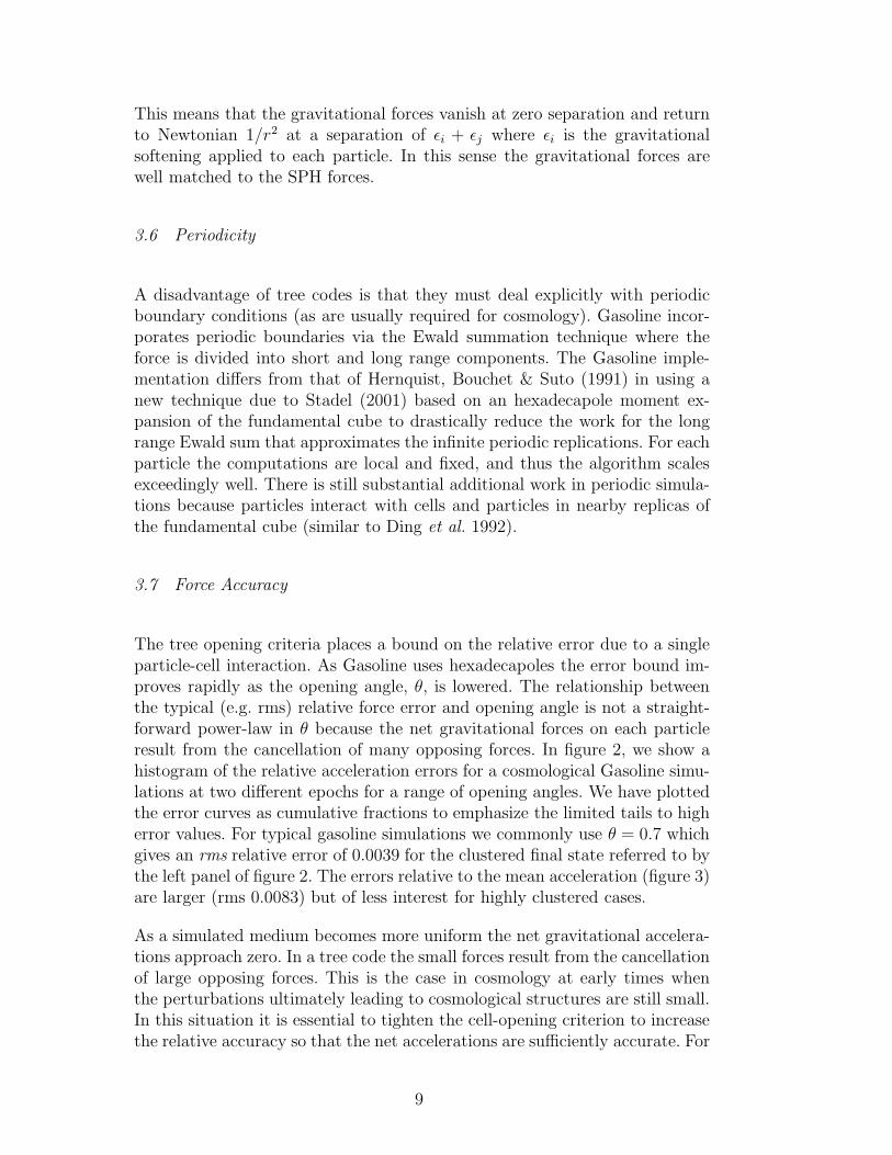
The tree opening criteria places a bound on the relative error due to a singleparticle-cell interaction. As Gasoline uses hexadecapoles the error bound im-proves rapidly as the opening angle, θ, is lowered. The relationship betweenthe typical (e.g. rms) relative force error and opening angle is not a straight-forward power-law in θ because the net gravitational forces on each particleresult from the cancellation of many opposing forces. In figure 2, we show ahistogram of the relative acceleration errors for a cosmological Gasoline simu-lations at two different epochs for a range of opening angles. We have plottedthe error curves as cumulative fractions to emphasize the limited tails to higherror values. For typical gasoline simulations we commonly use θ = 0.7 whichgives an rms relative error of 0.0039 for the clustered final state referred to bythe left panel of figure 2. The errors relative to the mean acceleration (figure 3)are larger (rms 0.0083) but of less interest for highly clustered cases.

As a simulated medium becomes more uniform the net gravitational accelera-tions approach zero. In a tree code the small forces result from the cancellationof large opposing forces. This is the case in cosmology at early times whenthe perturbations ultimately leading to cosmological structures are still small.In this situation it is essential to tighten the cell-opening criterion to increasethe relative accuracy so that the net accelerations are sufficiently accurate. For

9

10-5 10-4 10-3 10-2 10-1 100

Relative error, |δai|/|ai|

0.0001

0.0010

0.0100

0.1000

1.0000C

um

ula

tiv

e F

ract

ion

z=0

θ = 1.1

0.9

0.7

0.5

0.3

0.1

10-5 10-4 10-3 10-2 10-1 100

Relative error, |δai|/|ai|

0.0001

0.0010

0.0100

0.1000

1.0000

Cu

mu

lati

ve

Fra

ctio

n

z=19

θ = 1.1

0.9

0.7

0.5

0.4

0.30.1

Fig. 2. Gasoline relative errors, for various opening angles θ. The distributions areall for a 323, 64 Mpc box where the left panel represents the clustered final stateand the right an initial condition (redshift z = 19). Typical values of θ = 0.5 and0.7 are shown as thick lines. The solid curves compare to exact forces and thushave a minimum error set by the parameters of the Ewald summation whereasthe dotted curves compare to the θ = 0.1 case. The Ewald summation errors onlybecome noticeable for θ < 0.4. Relative errors are best for clustered objects butover-emphasize errors for low acceleration particles that are common in cosmologicalinitial conditions.

example in the right hand panels of figures 2 and 3 the errors are larger, and atz = 19, the rms relative error is 0.041 for θ = 0.7. However, here the absoluteerrors are lower by nearly a factor of two in rms (0.026) as shown in figure 3.At early times when the medium fairly homogeneous growth is driven by localgradients, and thus acceleration errors normalized to the mean accelerationprovide the better measure of accuracy as large relative errors are meaninglessfor accelerations close to zero. To ensure accurate integrations we switch tovalues such as θ = 0.5 before z = 2, giving an rms relative error of 0.0077 andan rms error of 0.0045 normalized to the mean absolute acceleration for thez = 19 distribution (a reasonable start time for a cosmological simulation onthis scale).

4 Gasdynamics

Astrophysical systems are predominantly at very low physical densities andexperience wide-ranging temperature variations. Most of the material is ina highly compressible gaseous phase. In general this means that a perfectadiabatic gas is an excellent approximation for the system. Microscopic phys-ical processes such as shear viscosity and diffusion can usually be neglected.

10

10-5 10-4 10-3 10-2 10-1 100

Error relative to mean, |δai|/<|a|>

0.0001

0.0010

0.0100

0.1000

1.0000C

um

ula

tiv

e F

ract

ion

z=0

θ = 1.1

0.9

0.7

0.5

0.3

0.1

10-5 10-4 10-3 10-2 10-1 100

Error relative to mean, |δai|/<|a|>

0.0001

0.0010

0.0100

0.1000

1.0000

Cu

mu

lati

ve

Fra

ctio

n

z=19

θ = 1.1

0.9

0.7

0.5

0.4

0.30.1

Fig. 3. Gasoline errors relative to the mean for the same cases as Fig. 2. The errorsare measured compared to the mean acceleration (magnitude) averaged over allthe particles. Errors relative to the mean are more appropriate to judge accuracyfor small accelerations resulting from force cancellation in a nearly homogeneousmedium.

High-energy processes and the action of gravity tend to create large veloci-ties so that flows are both turbulent and supersonic: strong shocks and veryhigh Mach numbers are common. Radiative cooling processes can also be im-portant; however, the timescales can often be much longer or shorter thandynamical timescales. In the latter case isothermal gas is often assumed forsimplicity. In many areas of computational astrophysics, particularly cosmol-ogy, gravity tends to be the dominating force that drives the evolution ofthe system. Visible matter, usually in the form of radiating gas, provides theessential link to observations. Radiative transfer is always present but maynot significantly affect the energy and thus pressure of the gas during thesimulation.

Fluid dynamics solvers can be broadly classified into Eulerian or Lagrangianmethods. Eulerian methods use a fixed computational mesh through whichthe fluid flows via explicit advection terms. Regular meshes provide for easeof analysis and thus high order methods such as PPM (Woodward & Collela1984) and TVD schemes (e.g. Harten et al. 1987, Kurganov & Tadmor 2000)have been developed. The inner loops of mesh methods can often be pipelinedfor high performance. Lagrangian methods follow the evolution of fluid parcelsvia the full (comoving) derivatives. This requires a deforming mesh or a mesh-less method such as Smoothed Particle Hydrodynamics (SPH) (Monaghan1992). Data management is more complex in these methods; however, advec-tion is handled implicitly and the simulation tends to naturally adapt to followdensity contrasts.

11

Large variations in physical length scales in astrophysics have limited the use-fulness of Eulerian grid codes. Adaptive Mesh Refinement (AMR) (Fryxell etal. 2000, Bryan & Norman 1997) overcomes this at the cost of data manage-ment overheads and increased code complexity. In the cosmological contextthere is the added complication of dark matter. There is more dark matterthan gas in the universe so it dominates the gravitational potential. Perturba-tions present on all scales in the dark matter guide the formation of gaseousstructures including galaxies and the first stars. A fundamental limit to AMRin computational cosmology is matching the AMR resolution to the underly-ing dark matter resolution. Particle based Lagrangian methods such as SPHare well matched to this constraint. A useful feature of Lagrangian simulationsis that bulk flows (which can be highly supersonic in the simulation frame) donot limit the timesteps. Particle methods are well suited to rapidly rotatingsystems such as astrophysical disks where arbitrarily many rotation periodsmay have to be simulated (e.g. SPH explicitly conserves angular momentum).A key concern for all methods is correct angular momentum transport.

5 Smoothed Particle Hydrodynamics in Gasoline

Smoothed Particle Hydrodynamics is an approach to hydrodynamical mod-elling developed by Lucy (1977) and Gingold & Monaghan (1977). It is aparticle method that does not refer to grids for the calculation of hydrody-namical quantities: all forces and fluid properties are found on moving particleseliminating numerically diffusive advective terms. The use of SPH for cosmo-logical simulations required the development of variable smoothing to handlehuge dynamic ranges (Hernquist & Katz 1989). SPH is a natural partnerfor particle based gravity. SPH has been combined with P3M (Evrard 1988),Adaptive P3M (HYDRA, Couchman et al. 1995), GRAPE (Steinmetz 1996)and tree gravity (Hernquist & Katz 1989). Parallel codes using SPH includeHydra MPI, Parallel TreeSPH (Dave, Dubinski & Hernquist 1997) and theGADGET tree code (Springel et al. 2001).

The basis of the SPH method is the representation and evolution of smoothlyvarying fluid quantities whose value is only known at disordered discrete pointsin space occupied by particles. Particles are the fundamental resolution ele-ments comparable to cells in a mesh. SPH functions through local summationoperations over particles weighted with a smoothing kernel, W , that approxi-mates a local integral. The smoothing operation provides a basis from which toobtain derivatives. Thus, estimates of density related physical quantities andgradients are generated. The summation aspect led to SPH being describedas a Monte Carlo type method (with O(1/

√N) errors) however it was shown

by Monaghan (1985) that the method is more closely related to interpolationtheory with errors O((lnN)d/N), where d is the number of dimensions.

12

A general smoothed estimate for some quantity f at particle i given particlesj at positions ~rj takes the form:

fi,smoothed =n∑

j=1

fjWij(~ri − ~rj, hi, hj), (2)

where Wij is a kernel function and hj is a smoothing length indicative ofthe range of interaction of particle j. It is common to convert this particle-weighted sum to volume weighting using fjmj/ρj in place of fj where the mj

and ρj are the particle masses and densities, respectively. For momentum andenergy conservation in the force terms, a symmetric Wij = Wji is required.We use the kernel-average first suggested by Hernquist & Katz (1989),

Wij =1

2w(|~ri − ~rj|/hi) +

1

2w(|~ri − ~rj|/hj) (3)

For w(x) we use the standard spline form with compact support where w = 0if x > 2 (Monaghan 1992).

We employ a fairly standard implementation of the the hydrodynamics equa-tions of motion for SPH (Monaghan 1992). Density is calculated from a sumover particle masses mj ,

ρi =n∑

j=1

mjWij. (4)

The momentum equation is expressed,

d~vidt

=−n∑

j=1

mj

(

Pi

ρ2i+

Pj

ρ2j+Πij

)

∇iWij , (5)

where Pj is pressure, ~vi velocity and the artificial viscosity term Πij is givenby,

Πij =

−α 1

2(ci+cj)µij+βµ2

ij1

2(ρi+ρj)

for ~vij · ~rij < 0,

0 otherwise,(6)

where µij =h(~vij · ~rij)

~r 2ij + 0.01(hi + hj)2

, (7)

where ~rij = ~ri − ~rj, ~vij = ~vi − ~vj and cj is the sound speed. α = 1 andβ = 2 are coefficients we use for the terms representing shear and Von

13

Neumann-Richtmyer (high Mach number) viscosities respectively. When sim-ulating strongly rotating systems we use the multiplicative Balsara (1995)

switch |∇·~v||∇·~v|+|∇×~v|

to suppress the viscosity in non-shocking, shearing environ-ments.

The pressure averaged energy equation (analogous to equation 5) conservesenergy exactly in the limit of infinitesimal time steps but may produce negativeenergies due to the Pj term if significant local variations in pressure occur. Weemploy the following equation (advocated by Evrard 1988, Benz 1989) whichalso conserves energy exactly in each pairwise exchange but is dependent onlyon the local particle pressure,

d ui

dt=

Pi

ρ2i

n∑

j=1

mj~vij · ∇iWij , (8)

where ui is the internal energy of particle i, which is equal to 1/(γ − 1)Pi/ρifor an ideal gas. In this formulation entropy is closely conserved making itsimilar to alternative entropy integration approaches such as that proposedby Springel & Hernquist (2002).

SPH derivative estimates, such as the rate of change of thermal energy, varysufficiently from the exact answer so that over a full cosmological simulationthe cooling due to universal expansion will be noticeably incorrect. In this casewe use comoving divergence estimates and add the cosmological expansionterm explicitly.

5.1 Neighbour Finding

Finding neighbours of particles is a useful operation. A neighbour list is es-sential to SPH, but it can also be a basis for other local estimates, suchas a dark matter density, as a first step in finding potential colliders orinteractors via a short range force. Stadel developed an efficient search al-gorithm using priority queues and a K-D tree ball-search to locate the k-nearest neighbours for each particle (freely available as the Smooth utility athttp://www-hpcc.astro.washington.edu). For Gasoline we use a parallelversion of the algorithm that caches non-local neighbours via MDL. The SPHinteraction distance 2hi is set equal to the k-th neighbour distance from par-ticle i. We use an exact number of neighbours. The number is set to a valuesuch as 32 or 64 at start-up. We have also implemented a minimum smoothinglength which is usually set to be comparable to the gravitational softening.

To calculate the fluid accelerations using SPH we perform two smoothing

14

operations. First we sum densities and then forces using the density estimates.To get a kernel-averaged sum for every particle (equations 2,3) it is sufficientto perform a gather operation over all particles within 2hi of every particle i. Ifonly a subset of the particles are active and require new forces, all particles forwhich the active set are neighbours must also perform a gather so that they canscatter their contribution to the active set. Finding these scatter neighboursrequires solving the k-inverse nearest neighbour problem, an active researcharea in computer science (e.g. Anderson & Tjaden 2001). Fortunately, duringa simulation the change per step in h for each particle typically less than2-3 percent, so it is sufficient to find scatter neighbours, j for which someactive particles is within 2hj,OLD(1+ e). We use a tree search where the nodescontain SPH interaction bounds for their particles estimated with e = 0.1.A similar scheme has been employed by Springel et al. (2001). For the forcessum the inactive neighbours need density values which can be estimated usingthe continuity equation or calculated exactly with a second inverse neighboursearch.

5.2 Cooling

In astrophysical systems the cooling timescale is usually short compared todynamical timescales which often results in temperatures that are close to anequilibrium set by competing heating and cooling processes. We have imple-mented a range of cases including: adiabatic (no cooling), isothermal (instantcooling), and implicit energy integration. Hydrogen and Helium cooling pro-cesses have been incorporated. Ionization fractions are calculated assumingequilibrium for efficiency. Gasoline optionally adds heating due to feedbackfrom star formation, an uniform UV background or using user defined func-tions.

The implicit integration uses a stiff equation solver assuming that the hydrody-namic work and density are constant across the step. The second order natureof the particle integration is maintained using an implicit predictor step whenneeded. Internal energy is required on every step to calculate pressure forceson the active particles. The energy integration is O(N) but reasonably expen-sive. To avoid integrating energy for every particle on the smallest timestepwe extrapolate each particle forward on its individual dynamical timestep anduse linear interpolation to estimate internal energy at intermediate times asrequired.

15

Full Step: Kick Drift Kick Full Step: Drift Kick Drift

Rung 0 (Base time step)

Rung 1

Rung 2

Rung 0 (Base time step)

Rung 1

Rung 2

Fig. 4. Illustration of multiple timestepping: the linear sections represent particlepositions during a Drift step with time along the x-axis. The vertical bars representKicks changing the velocity. In KDK, the accelerations are applied as two half-kicks(from only one force evaluation) which is why there are two bars interior of theKDK case. At the end of each full step all variables are synchronised.

6 Integration: Multiple Timesteps

The range of physical scales in astrophysical systems is large. For examplecurrent galaxy formation simulations contain 9 orders of magnitude variationin density. The dynamical timescale for gravity scales as ρ−1/2 and for gas itscales as ρ−1/3 T−1/2. For an adiabatic gas the local dynamical time scalesas ρ−2/3. With gas cooling (or the isothermal assumption) simulations canachieve very high gas densities. In most cases gas sets the shortest dynam-ical timescales, and thus gas simulations are much more demanding (manymore steps to completion) than corresponding gravity only simulations. Timeadaptivity can be very effective in this regime.

Gasoline incorporates the timestep scheme described as Kick-Drift-Kick (KDK)in Quinn et al. (1997). The scheme uses a fixed overall timestep. Starting withall quantities synchronised, velocities and energies are updated to the half-step (half-Kick), followed by a full step position update (Drift). The positionsalone are sufficient to calculate gravity at the end of the step; however, forSPH, velocities and thermal energies are also required and obtained with apredictor step using the old accelerations. Finally another half-Kick is appliedsynchronising all the variables. Without gas forces this is a symplectic leap-frog integration. The leap-frog scheme requires only one force evaluation andminimum storage. While symplectic integration is not required in cosmology itis critical in solar system integrations or any system where natural instabilitiesoccur over very many dynamical times.

An arbitrary number of sub-stepping rungs factors of two smaller may be usedas shown in Figure 4. The scheme is no longer strictly symplectic if particleschange rungs during the integration which they generally must do to satisfytheir individual timestep criteria. After overheads, tree-based force calculationscales approximately with the number of active particles so large speed-upsmay be realised in comparison to single stepping (see section 7). Figure 4

16

compares KDK with Drift-Kick-Drift (DKD), also discussed in Quinn et al.

(1997). For KDK the force calculations for different rungs are synchronised. Inthe limit of many rungs this results in half as many force calculation times withtheir associated tree builds compared to DKD. KDK also gives significantlybetter momentum and energy conservation for the same choice of timestepcriteria.

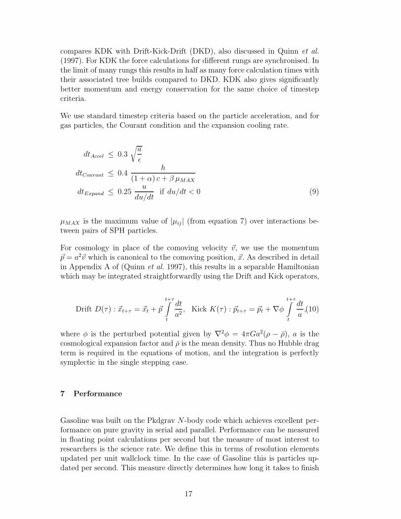
We use standard timestep criteria based on the particle acceleration, and forgas particles, the Courant condition and the expansion cooling rate.

dtAccel ≤ 0.3

√

a

ǫ

dtCourant ≤ 0.4h

(1 + α) c+ β µMAX

dtExpand ≤ 0.25u

du/dtif du/dt < 0 (9)

µMAX is the maximum value of |µij| (from equation 7) over interactions be-tween pairs of SPH particles.

For cosmology in place of the comoving velocity ~v, we use the momentum~p = a2~v which is canonical to the comoving position, ~x. As described in detailin Appendix A of (Quinn et al. 1997), this results in a separable Hamiltonianwhich may be integrated straightforwardly using the Drift and Kick operators,

Drift D(τ) : ~xt+τ = ~xt + ~p

t+τ∫

t

dt

a2, Kick K(τ) : ~pt+τ = ~pt +∇φ

t+τ∫

t

dt

a,(10)

where φ is the perturbed potential given by ∇2φ = 4πGa2(ρ − ρ), a is thecosmological expansion factor and ρ is the mean density. Thus no Hubble dragterm is required in the equations of motion, and the integration is perfectlysymplectic in the single stepping case.

7 Performance

Gasoline was built on the Pkdgrav N -body code which achieves excellent per-formance on pure gravity in serial and parallel. Performance can be measuredin floating point calculations per second but the measure of most interest toresearchers is the science rate. We define this in terms of resolution elementsupdated per unit wallclock time. In the case of Gasoline this is particles up-dated per second. This measure directly determines how long it takes to finish

17

0 20 40 60 80 100Number of Alpha Processors

0

5.0•104

1.0•105

1.5•105

2.0•105P

arti

cles

per

sec

on

dSPHSPH+TreeBuild

GravityGravity+TreeBuild

Overall

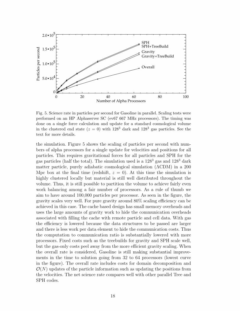
Fig. 5. Science rate in particles per second for Gasoline in parallel. Scaling tests wereperformed on an HP Alphaserver SC (ev67 667 MHz processors). The timing wasdone on a single force calculation and update for a standard cosmological volumein the clustered end state (z = 0) with 1283 dark and 1283 gas particles. See thetext for more details.

the simulation. Figure 5 shows the scaling of particles per second with num-bers of alpha processors for a single update for velocities and positions for allparticles. This requires gravitational forces for all particles and SPH for thegas particles (half the total). The simulation used is a 1283 gas and 1283 darkmatter particle, purely adiabatic cosmological simulation (ΛCDM) in a 200Mpc box at the final time (redshift, z = 0). At this time the simulation ishighly clustered locally but material is still well distributed throughout thevolume. Thus, it is still possible to partition the volume to achieve fairly evenwork balancing among a fair number of processors. As a rule of thumb weaim to have around 100,000 particles per processor. As seen in the figure, thegravity scales very well. For pure gravity around 80% scaling efficiency can beachieved in this case. The cache based design has small memory overheads anduses the large amounts of gravity work to hide the communication overheadsassociated with filling the cache with remote particle and cell data. With gasthe efficiency is lowered because the data structures to be passed are largerand there is less work per data element to hide the communication costs. Thusthe computation to communication ratio is substantially lowered with moreprocessors. Fixed costs such as the treebuilds for gravity and SPH scale well,but the gas-only costs peel away from the more efficient gravity scaling. Whenthe overall rate is considered, Gasoline is still making substantial improve-ments in the time to solution going from 32 to 64 processors (lowest curvein the figure). The overall rate includes costs for domain decomposition andO(N) updates of the particle information such as updating the positions fromthe velocities. The net science rate compares well with other parallel Tree andSPH codes.

18

1 1/2 1/4 1/8 1/16 1/32 1/64 1/128Timestep Bin

0

1000

2000

3000

4000

Wo

rk p

er b

in (

seco

nd

s)Single-stepping: every particle on smallest timestep

Individual timesteps (Gasoline)

Individual timesteps, lowered fixed cost

Individual timesteps, perfect cost scaling

Fig. 6. Benefits of multistepping. Each major timestep is performed as a hierarchicalsequence of substeps with varying numbers of particles active in each timestep bin.We are using a realistic case: a single major step of a galaxy simulation at redshiftz = 1 (highly clustered) run on 8 alpha processors with a range of 128 in timesteps.Gasoline (solid line) achieves an overall 4.1 times speed-up over a single steppingcode (dashed line). Planned improvements in the fixed costs such as tree building(dotted line) would give a 5.3 times speedup. If all costs could be scaled to thenumber of particles in each timestep bin (dash-dot line), the result would be a 9.5times speed-up over single stepping.

Figure 5 only treats single timestepping. Multiple timesteps provide an ad-ditional speed-up in the science rate of a factor typically in the range of 2-5that is quite problem dependent. The value of individual particle timesteps isillustrated separately in figure 6. For this example we analysed the time spentby Gasoline doing a single major step (around 13 Million years) of a millionparticle Galaxy formation simulation at redshift z = 1. The simulation useda range of 128 in substeps per major step. The top curve in the figure is thecost for single stepping. It rises exponentially, doubling with every new bin,and drops off because the last bin was not always occupied. Sample numbersof particles in the bins (going from 0 to 7) were 473806, 80464, 63708, 62977,85187, 129931, 1801 and 20 respectively. Using individual timesteps Gasolinewas running 4 times faster than an equivalent single stepping code. The testwas performed in parallel on 8 processors, and it is heartening that despitethe added difficulties of load balancing operations on subsets of the particlesthe factor of 4 benefit was realized. Tree building and other fixed costs thatdo not scale with the number of active particles can be substantially reducedusing tree-repair and related methods (e.g. Springel et al. 2001) which wouldbring the speed-up to around 5. In the limit of uniform costs per particle inde-pendent of the number of active particles the speed-up would approach 10. Inthis example the timestep range was limited partly due to restrictions imposedon the SPH smoothing length. In future work we anticipate a wider range of

19

timestep bins. With a few particles consistently on a timestep 1/256th of themajor step the theoretical speed-up factor is over 30. In practice, overheadswill always limit the achievable speed-up. In the limit of very large numbers ofrungs the current code would asymptotically approach a factor of 10 speedup.With the fixed costs of tree builds and domain decomposition made to scalewith the number of active particles (e.g. tree-repair), the asymptotic speedup achievable with Gasoline would be 24 times. The remaining overheads areincreasingly difficult to address. For small runs, such as the galaxy formationexample used here, the low numbers of the particles on the shortest timestepsmake load balancing difficult. If more than 16 processors are used with thecurrent code on this run there will be idle processors for a noticeable fractionof the time. Though the time to solution is reduced with more processors, itis an inefficient use of computing resources. The ongoing challenge is to see ifbetter load balance through more complex work division offsets increases incommunication and other parallel overheads.

8 Tests

-6 -4 -2 0 2 4 60.0

0.2

0.4

0.6

0.8

1.0

1.2

Den

sity

-6 -4 -2 0 2 4 60.0

0.2

0.4

0.6

0.8

1.0

Vel

oci

ty

Fig. 7. Sod (1978) shock tube test results with Gasoline for density (left) and ve-locity (right). This a three dimensional test using glass initial conditions similarto the conditions in a typical simulation. The diamonds represent averages in binsseparated by the local particle spacing: the effective fluid element width. Discon-tinuities are resolved in 3-4 particle spacings which is much fewer than in the onedimensional results shown in Hernquist & Katz (1989).

20

8.1 Shocks: Spherical Adiabatic Collapse

There are three key points to keep in mind when evaluating the performanceof SPH on highly symmetric tests. The first is that the natural particle config-uration is a semi-regular three dimensional glass rather than a regular mesh.The second is that individual particle velocities are smoothed before they af-fect the dynamics so that the low level noise in individual particle velocities isnot particularly important. The dispersion in individual velocities is related tocontinuous settling of the irregular particle distribution. This is particularlyevident after large density changes. Thirdly, the SPH density is a smoothedestimate. Any sharp step in the number density of particles translates into adensity estimate that is smooth on the scale of ∼ 2 − 3 particle separations.When relaxed irregular particle distributions are used, SPH resolves densitydiscontinuities close to this limit. As a Lagrangian method SPH can also re-solve contact discontinuities just as tightly without the advective spreading ofsome Eulerian methods.

We have performed standard Sod (1978) shock tube tests used for the originalTreeSPH (Hernquist & Katz 1989). We find the best results with the pairwiseviscosity of equation 7 which is marginally better than the bulk viscosity for-mulation for this test . The one dimensional tests often shown do not properlyrepresent the ability of SPH to model shocks on more realistic problems. Theresults of figure 7 demonstrate that SPH can resolve discontinuities in a shocktube very well when the problem is setup to be comparable to the environmentin a typical three dimensional simulation.

The shocks of the previous example have a fairly low Mach number comparedto astrophysical shocks found in collapse problems. (Evrard 1988) first intro-duced a spherical adiabatic collapse as a test of gasdynamics with gravity.This test is nearly equivalent to the self-similar collapse of Navarro & White(1993) and has comparable shock strengths. We compare Gasoline results onthis problem with very high resolution 1D Lagrangian mesh solutions in fig-ure 8. We used a three-dimensional glass initial condition. The solution isexcellent with 2 particle spacings required to model the shock. The deviationat the inner radii is a combination of the minimum smoothing length (0.01)and earlier slight over-production of entropy at a less resolved stage of the col-lapse. The pre-shock entropy generation (bottom left panel of Fig. 8 occurs inany strongly collapsing flow and is present for both the pairwise (equation 7)and divergence based artificial viscosity formulations. The post-shock entropyvalues are correct.

21

0.01 0.10 1.000.1

1.0

10.0

100.0

1000.0

Density

0.01 0.10 1.000.01

0.10

1.00

10.00

100.00

1000.00

Pressure

0.01 0.10 1.00

0.01

0.10

Entropy

0.01 0.10 1.00

-1.5

-1.0

-0.5

0.0

Velocity

Fig. 8. Adiabatic collapse test from Evrard (1988) with 28000 particles, shown attime t = 0.8 (t = 0.88 in Hernquist & Katz, 1989). The results shown as diamondsare binned at the particle spacing with actual particle values shown as points. Thesolid line is a high resolution 1D PPM solution provided by Steinmetz.

8.2 Rotating Isothermal Cloud Collapse

The rotating isothermal cloud test examines the angular momentum transportin an analogue of a typical astrophysical collapse with cooling. Grid methodsmust explicitly advect material across cell boundaries which leads to small butsystematic angular momentum non-conservation and transport errors. SPHconserves angular momentum very well, limited only by the accuracy of thetime integration of the particle trajectories. However, the SPH artificial viscos-ity that is required to handle shocks has an unwanted side-effect in the formof viscous transport away from shocks. The magnitude of this effect scalingwith the typical particle spacing, and it can be combatted effectively with in-creased resolution. The Balsara (1995) switch detects shearing regions so thatthe viscosity can be reduced where strong compression is not also present.

We modelled the collapse of a rotating, isothermal gas cloud. This test issimilar to a tests performed by (Navarro & White 1993) and (Thacker et

al. 2000) except that we have simplified the problem in the manner of (Navarro& Steinmetz 1997). We use a fixed (Navarro, Frenk and White 1995) (con-centration c=11, Mass=2 × 1012M⊙) potential without self-gravity to avoid

22

Half Angular Momentum Radius

0 2 4 6 8 10 12Time (Gyr)

0102030400

102030400

102030400

1020304050

kp

c

64 particles

125 particles

501 particles

4049 particles

Fig. 9. Angular Momentum Transport as a function of resolution tested through thecollapse of an isothermal gas cloud in a fixed potential. The methods representedare: Monaghan viscosity with the Balasara switch (thick solid line), bulk viscosity(thick dashed line), Monaghan viscosity (thin line) and Monaghan Viscosity withoutmultiple timesteps (thin dotted line).

coarse gravitational clumping with associated angular momentum transport.This results in a disk with a circular velocity of 220 km/s at 10 kpc. The4×1010M⊙, 100 kpc gas cloud was constructed with particle locations evolvedinto a uniform density glass initial condition and set in solid body rotation(~v = 0.407 km/s/pc ez × ~r) corresponding to a rotation parameter λ ∼ 0.1.The gas was kept isothermal at 10, 000 K rather than using a cooling functionto make the test more general. The corresponding sound speed of 10 km/simplies substantial shocking during the collapse.

We ran simulations using 64, 125, 500 and 4000 particle clouds for 12 Gyr(43 rotation periods at 10 kpc). We present results for Monaghan viscosity,bulk viscosity (Hernquist-Katz) and our default set-up: Monaghan viscositywith the Balsara switch. Results showing the effect of resolution are shown infigure 9. Both Monaghan viscosity with the Balsara switch and bulk viscos-ity result in minimal angular momentum transport. The Monaghan viscositywithout the switch results in steady transport of angular momentum outwardswith a corresponding mass inflow. The Monaghan viscosity case was run withand without multiple timesteps. With multiple timesteps the particle momen-tum exchanges are no longer explicitly synchronized and the integrator is no

23

Half Mass Radius

0.0 0.5 1.0 1.5Time (Gyr)

0

20

40

60

80

100

kp

c

Half Ang Mom Radius

0.0 0.5 1.0 1.5Time (Gyr)

0

20

40

60

80

100

kp

c

Fig. 10. Angular Momentum Transport test: The initial collapse phase for the 4000particle collapse shown in figure 9. The methods represented are: Monaghan vis-cosity with the Balasara switch (thick solid line) and bulk viscosity (thick dashedline). Note the post-collapse bounce for the bulk viscosity.

longer perfectly symplectic. Despite this the evolution is very similar, particu-larly at high resolution. The resolution dependence of the artificial viscosity isimmediately apparent as the viscous transport drastically falls with increasingparticle numbers. It is worth noting that in hierarchical collapse processes thefirst collapses always involve small particle numbers. Our results are consistentwith the results of (Navarro & Steinmetz 1997). In that paper self-gravity ofthe gas was also included, providing an additional mechanism to transport an-gular momentum due to mass clumping. As a result, their disks show a gradualtransport of angular momentum even with the Balsara switch; however, thistransport was readily reduced with increased particle numbers.

In figure 10 we focus on the bounce that occurs during the collapse using bulkviscosity. Bulk viscosity converges very slowly towards the correct solutionand displays unwanted numerical behaviours even at high particle numbers.In cosmological adiabatic tests it tends to generate widespread heating duringthe early (pre-shock) phases of collapse. Thus we favour Monaghan artificialviscosity with the Balsara switch.

8.3 Cluster Comparison

The Frenk et al. (1999) cluster comparison involved simulating the formationof an extremely massive galaxy cluster with adiabatic gas (no cooling). Profilesand bulk properties of the cluster were compared for many widely used codes.We ran this cluster with Gasoline at two resolutions: 2 × 643 and 2 × 1283.

24

1.0

1.1

1.2

1.3m

tot [

1015

Msu

n ] (a)

850

900

950

1000

σ DM

[ k

m s

-1] (b)

0.08

0.10

0.12

mg

as /

mto

t

(c)

0.04 0.00 -0.04

0.50

0.55

0.60

Tg

as [

108 K

]

Redshift, z

(d)

Jen

kin

sB

ryan

Nav

arro

Wad

sley

Co

uch

man

Ste

inm

etz

Pen

Ev

rard

Gn

edin

Ow

enC

enY

epes

1.0

1.1

1.2

β

(e)

0.10

0.15

0.20

Uk

in/

Uth

erm

(f)

0.5

1.0

1.5

2.0

2.5

3.0

LX [

1031

Msu

n2 K

1/2 /

Mp

c3 ]

(g)

0.04 0.00 -0.041.0

1.2

1.4

1.6a/

b a

nd

a/

c

Redshift, z

(h)

Jen

kin

sB

ryan

Nav

arro

Wad

sley

Co

uch

man

Ste

inm

etz

Pen

Ev

rard

Gn

edin

Ow

enC

enY

epes

Fig. 11. Bulk Properties for the cluster comparison. All quantities are computedwithin the virial radius (2.74 Mpc for the gasoline runs). From top to bottom, theleft column gives the values of: (a) the total cluster mass; (b) the one-dimensional ve-locity dispersion of the dark matter; (c) the gas mass fraction; (d) the mass-weightedgas temperature. Also from top to bottom, the right column gives the values of: (e)β = mp/3kT ; (f) the ratio of bulk kinetic to thermal energy in the gas; (g) the X-rayluminosity; (h) the axial ratios of the dark matter (diamonds) and gas (crosses) dis-tributions. Gasoline results at 643 (solid) and 1283 (dashed) resolution are shownover a limit redshift range near z = 0, illustrating issues with timing discussed inthe text. The original paper simulation results at z = 0 are shown on the right ofeach panel (in order of decreasing resolution, left to right).

These were the two resolutions which other SPH codes used in the originalpaper. Profiles of the simulated cluster have previously been shown in Borganiet al. (2002). As shown in figure 11, the Gasoline cluster bulk properties arewithin the range of values for the other codes at z = 0. The Gasoline X-rayluminosity is near the high end; however, the results are consistent with thoseof the other codes.

The large variation in the bulk properties among codes was a notable resultof the original comparison paper. We investigated the source of this variationand found that a large merger was occurring at z = 0 with a strong shockat the cluster centre. The timing of this merger is significantly changed from

25

code-to-code or even within the same code at different resolutions as notedin the original paper. Running the cluster with Gasoline with 2 × 643 (solid)instead 2×1283 (dotted) particles changes the timing noticeably. The differentresolutions have modified initial waves which affect overall timing and levelsof substructure. These differences are highlighted by the merger event nearz = 0. As shown in the figure, the bulk properties are changing very rapidly ina short time. This appears to explain a large part of the code-to-code variationin quantities such as mean gas temperature and the kinetic to thermal energyratio. Timing issues are likely to be a feature of future cosmological codecomparisons.

9 Applications and discussion

The authors have applied Gasoline to provide new insight into clusters ofgalaxies, dwarf galaxies, galaxy formation, gas-giant planet formation andlarge scale structure. These applications are a testament to the robustness,flexibility and performance of the code.

Mayer, Quinn, Wadsley & Stadel (2002) used Gasoline at high resolution toshow convincingly that giant planets can form in marginally unstable disksaround protostars in just a few orbital periods. These simulation used 1 milliongas particles and were integrated for around thousand years until dense proto-planets formed. Current work focusses on improving the treatment of theheating and cooling processes in the disk.

Borgani et al.(2001,2002) used Gasoline simulations of galaxy clusters in thestandard ΛCDM cosmology to demonstrate that extreme levels of heating inexcess of current estimates from Supernovae associated with the current stellarcontent of the universe are required to make cluster X-ray properties matchobservations. The simulations did not use gas cooling, and this is a next step.

Governato et al. (2002) used Gasoline with star formation algorithms to pro-duce a realistic disk galaxy in the standard ΛCDM cosmology. Current workaims to improve the resolution and the treatment of the star formation pro-cesses.

Mayer et al.(2001a,b) simulated the tidal disruption of dwarf galaxies aroundtypical large spiral galaxy hosts (analogues of the Milky Way), showing theexpected morphology of the gas and stellar components.

Bond et al. (2002) used a 270 million particle cosmological Gasoline simulationto provide detailed estimates of the Sunyaev-Zel’dovich effect on the cosmicmicrowave background at small angular scales. This simulated 400 Mpc cube

26

contains thousands of bright X-ray clusters and provides a statistical sam-ple that is currently being matched to observational catalogues (Wadsley &Couchman 2003).

A common theme in these simulations is large dynamic ranges in space andtime. These represent the cutting edge for gasdynamical simulations of self-gravitating astrophysical systems, and were enabled by the combination ofthe key features of Gasoline described above. The first feature is simply oneof software engineering: a modular framework had been constructed in orderto ensure that Pkdgrav could both scale well, but also be portable to manyparallel architectures. Using this framework, it was relatively straightforwardto include the necessary physics for gasdynamics. Of course, the fast, adapt-able, parallel gravity solver itself is also a necessary ingredient. Thirdly, thegasdynamical implementation is state-of-the-art and tested on a number ofstandard problems. Lastly, significant effort has gone into making the codeadaptable to a large range in timescales. Increasing the efficiency with whichsuch problems can be handled will continue be a area of development withcontributions from Computer Science and Applied Mathematics.

10 Acknowledgments

The authors would like to thank Carlos Frenk for providing the cluster compar-ison results and Matthias Steinmetz for providing high resolution results forthe spherical collapse. Development of Pkdgrav and Gasoline was supportedby grants from the NASA HPCC/ESS program.

References

Aarseth, S., Lecar, M. 1975, ARAA, 13, 1

Bagla, J.S., 2002, J. Astrophysics and Astronomy 23, 185

Balsara, D. S., 1995, J. Computational Physics, 121, 2, 357-372

Benz, W., 1989, “Numerical Modelling of Stellar Pulsation”, Nato Workshop, LesArcs, France

Bentley, J.L. 1979, IEEE Transactions on Software Engineering, SE-5(4), 333

Bode, P., Ostriker, J.P., Xu G., 2000 ApJS, 128, 561

Bond, J., Contaldi, C., Pen, U-L., Pogosyan, D., Prunet, S., Ruetalo, M., Wadsley,J., Zhang, P., Mason, B., Myers, S., Pearson, T., Readhead, A., Sievers, J.,Udomprasert, P. 2002, ApJ (submitted), astro-ph/0205386

27

Borgani, S., Governato, F., Wadsley, J., Menci, N., Tozzi, P., Quinn, T., Stadel, J.,Lake, G. 2002, MNRAS, 336, 409

Borgani, S., Governato, F., Wadsley, J., Menci, N., Tozzi, P., Lake, G., Quinn, T.,Stadel, J. 2001, ApJ, 559, 71

Bryan, G. & Norman, M. 1997, in Computational Astrophysics, Proc. 12th KingstonConference, Halifax, Oct. 1996, ed. D. Clarke & M. West (PASP), p. 363

Couchman, H.M.P. 1991, ApJL, 368, 23

Couchman, H. M. P., Thomas, P. A., Pearce, F. R. 1995, ApJ, 452, 797

Dave, R., Dubinksi, J. & Hernquist, L. 1997, NewA, 2, 277

Dehnen, W. 2000, ApJ, 536, 39

Ding, H., Karasawa, N., and Goddard III, W. 1992, Chemical Physics Letters, 196(1,2), 6–10.

Efstathiou, G., Davis, M., Frenk, C.S., White, S.D.M. 1985, ApJS, 57, 241

Evrard, A. E. 1988, Monthly Notices R.A.S., 235, 911

Fryxell, B., Olson, K., Ricker, P., Timmes, F. X., Zingale, M., Lamb, D. Q.,MacNeice, P., Rosner, R., Truran, J. W., Tufo, H. 2000, ApJS, 131, 273,http://flash.uchicago.edu

Frenk, C., White, S., Bryan, G., Norman, M., Cen, R., Ostriker, G., Couchman, H.,Evrard, G., Gnedin, N., Jenkins, A., Pearce, F., Thomas, P., Navarro, H., Owen,J., Villumsen, J., Pen, U-L., Steinmetz, M., Warren, J., Zurek, w., Yepes, G. &Klypin, A., 1999, Ap. J., 525, 554

Gingold, R.A. & Monaghan, J.J. 1977, Monthly Notices R.A.S., 181, 375

Governato, F., Mayer, L., Wadsley, J., Gardner, J.P., Willman, B., Hayashi, E.,Quinn, T., Stadel, J., Lake, G. 2002, ApJ (submitted), astro-ph/0207044

Greengard, L. and Rokhlin, V. 1987, J. Comput. Phys., 73, 325

Harten, A., Enquist, B., Osher, S. and Charkravarthy, S., 1987, J. Comput. Phys.,71, 231-303

Hernquist, L. & Katz, N. 1989, Astrophysical Journal Supp., 70, 419

Hernquist, L., Bouchet, F., and Suto, Y. 1991, ApJS, 75, 231-240

Hernquist, L. and Ostriker, J. 1992, ApJ, 386, 375

Homberg, Erik 1947, Astrophysical Journal, 94, 385

Hockney, R.W. & Eastwood, J.W. 1988, Computer Simulation using Particles, IOPPublishing

Hut, P. and Makino, J. 1999, Science,283, 501

28

Jernigan, J.G. and Porter, D.H. 1989, ApJS, 71, 871

Joe, B. (1989), “Three-dimensional triangulations from local transformations”,SIAM J. Sci. Stat. Comput., 10, pp. 718-741.

Kravtsov, A.V., Klypin, A.A. and Khokhlov, A.M.J. 1997, ApJS, 111, 73

Kurganov, A. and Tadmor, E, 2000, J. Comput. Phys., 160, 241

Lucy, L. 1977, Astronomical Journal, 82, 1013

Mayer, L., Quinn, T., Wadsley, J., Stadel, J. 2002, Science, 298, 1756

Mayer, L., Governato, F., Colpi, M., Moore, B., Quinn, T., Wadsley, J., Stadel, J.,Lake, G. 2001, ApJ, 559, 754

Mayer, L., Governato, F., Colpi, M., Moore, B., Quinn, T., Wadsley, J., Stadel, J.,Lake, G. 2001, ApJ, 547, 123

Monaghan, J.J. 1985, Computer Physics Reports, 3, 71

Monaghan, J.J. 1992, Annual Reviews in Astronomy and Astrophysics, 30, 543

Navarro, J.F. & White S.D.M 1993, Monthly Notices R.A.S., 265, 271

Navarro, J.F., Frenk, C. & White S.D.M 1995, Monthly Notices R.A.S., 275, 720

Navarro, J.F. & Steinmetz, M. 1997, Astrophysical Journal, 478, 13

Press, W.H., Teukolsky, S.A., Vetterling W.T., Flannery, B.P. 1995, NumericalRecipies in C, Cambridge University Press

Quinn, T., Katz, N., Stadel, J. & Lake, G. 1997, ApJ (submitted), astro-ph/9710043

Salmon, J. and Warren, M. 1994, J. Comput. Phys., 111, 136

Sod, G.A. 1978, Journal of Computational Physics, 27, 1

Springel, V., Yoshida, N., White, S.D.M. 2001, New A., 6, 79

Springel, V. and Hernquist, L. 2002, MNRAS, 333, 649

Ph.D. Thesis, University of Washington, Seattle, WA, USA

Steinmetz, M. 1996, MNRAS, 278, 1005

Steinmentz, M. & Muller, E. 1993, Astronomy and Astropysics, 268, 391

Thacker, R., Tittley, E., Pearce, F., Couchman, H., and Thomas, P. 2000, Monthly

Notices R.A.S., 319, 619

Anderson, R. & Tjaden, B. 2001, “The inverse nearest neighbor problem withastrophysical applications”, Proceedings of the Twelfth Annual ACM-SIAMSymposium on Discrete Algorithms (SODA), January 2001.

Wadsley, J.W., 1998, Ph.D. Thesis, University of Toronto, ON, Canada

29

Wadsley, J & Couchman, H., in preparation

Woodward, P. & Collela, P. 1984, Journal of Computational Physics, 54, 115

Richardson, D. C., Quinn, T., Stadel, J., and Lake, G. 2000, Icarus 143, 45–59.

Leinhardt, Z. M., Richardson, D. C., and Quinn, T. 2000, Icarus, 146, 133

Barnes, J., and Hut, P. 1986, Nature, 324:446–449.

Weinberg, M., 1999, Astron. J., 117, 629

30