GARCH Models - unipveconomia.unipv.it/pagp/pagine_personali/.../Rossi_GARCH_Ec_Fin_20… · Stylized Facts Stylized Facts GARCH models have been developed to account for empirical

GARCH Models

Eduardo RossiUniversity of Pavia

December 2013

Rossi GARCH Financial Econometrics - 2013 1 / 50

Outline

1 Stylized Facts

2 ARCH model: definition

3 GARCH model

4 EGARCH

5 Asymmetric Models

6 GARCH-in-mean model

7 The News Impact Curve


Stylized Facts

Stylized Facts

GARCH models have been developed to account for empirical regularities infinancial data. Many financial time series have a number of characteristics incommon.

Asset prices are generally non stationary. Returns are usually stationary.Some financial time series are fractionally integrated.

Return series usually show no or little autocorrelation.

Serial independence between the squared values of the series is often rejectedpointing towards the existence of non-linear relationships between subsequentobservations.


Stylized Facts

Stylized Facts

Volatility of the return series appears to be clustered.

Normality has to be rejected in favor of some thick-tailed distribution.

Some series exhibit so-called leverage effect, that is changes in stock pricestend to be negatively correlated with changes in volatility. A firm with debtand equity outstanding typically becomes more highly leveraged when thevalue of the firm falls.This raises equity returns volatility if returns areconstant. Black, however, argued that the response of stock volatility to thedirection of returns is too large to be explained by leverage alone.

Volatilities of different securities very often move together.


ARCH model: definition

The ARCH Model

ARCH process

(Bollerslev, Engle and Nelson, 1994) The process {εt (θ0)} follows an ARCH(AutoRegressive Conditional Heteroskedasticity) model if

Et−1 [εt (θ0)] = 0 t = 1, 2, . . .

and the conditional variance

σ2t (θ0) ≡ Vart−1 [εt (θ0)] = Et−1

[ε2t (θ0)

]t = 1, 2, . . .

depends non trivially on the σ-field generated by the past observations:{εt−1 (θ0) , εt−2 (θ0) , . . .} .



The ARCH Model

Let {yt (θ0)} denote the stochastic process of interest with conditional mean

µt (θ0) ≡ Et−1 (yt) t = 1, 2, . . .

µt (θ0) and σ2t (θ0) are measurable with respect to the time t − 1 information set.

Define the {εt (θ0)} process by

εt (θ0) ≡ yt − µt (θ0) .



The ARCH Model

It follows from eq.(5) and (5), that the standardized process

zt (θ0) ≡ εt (θ0)σ2t (θ0)−1/2 t = 1, 2, . . .

with

Et−1 [zt (θ0)] = 0

Vart−1 [zt (θ0)] = 1

will have conditional mean zero (Et−1 [zt (θ0)] = 0) and a time invariantconditional variance of unity.



The ARCH Model

We can think of εt (θ0) as generated by

εt (θ0) = zt (θ0)σ2t (θ0)1/2

where ε2t (θ0) is unbiased estimator of σ2

t (θ0).Let’s suppose zt (θ0) ∼ NID (0, 1) and independent of σ2

t (θ0)

Et−1

[ε2t

]= Et−1

[σ2t

]Et−1

[z2t

]= Et−1

[σ2t

]= σ2

t

because z2t |Φt−1 ∼ χ2

(1).



The ARCH Model

If the conditional distribution of zt is time invariant with a finite fourth moment,the fourth moment of εt is

E[ε4t

]= E

[z4t

]E[σ4t

]≥ E

[z4t

]E[σ2t

]2= E

[z4t

]E[ε2t

]2where the last equality follows from

E [σ2t ] = E [Et−1(ε2

t )] = E [ε2t ]

E[ε4t

]≥ E

[z4t

]E[ε2t

]2by Jensen’s inequality. The equality holds true for a constant conditional varianceonly.



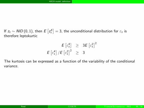
If zt ∼ NID (0, 1), then E[z4t

]= 3, the unconditional distribution for εt is

therefore leptokurtic

E[ε4t

]≥ 3E

[ε2t

]2E[ε4t

]/E[ε2t

]2 ≥ 3

The kurtosis can be expressed as a function of the variability of the conditionalvariance.



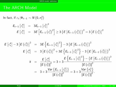
The ARCH Model

In fact, if εt |Φt−1 ∼ N(0, σ2

t

)Et−1

[ε4t

]= 3Et−1

[ε2t

]2E[ε4t

]= 3E

[Et−1

(ε2t

)2]≥ 3

{E[Et−1

(ε2t

)]}2= 3

[E(ε2t

)]2E[ε4t

]− 3

[E(ε2t

)]2= 3E

{Et−1

[ε2t

]2}− 3{E[Et−1

(ε2t

)]}2

E[ε4t

]= 3

[E(ε2t

)]2+ 3E

{Et−1

[ε2t

]2}− 3{E[Et−1

(ε2t

)]}2

k =E[ε4t

][E (ε2

t )]2 = 3 + 3

E{Et−1

[ε2t

]2}− {E [Et−1

(ε2t

)]}2

[E (ε2t )]

2

= 3 + 3Var

{Et−1

[ε2t

]}[E (ε2

t )]2 = 3 + 3

Var{σ2t

}[E (ε2

t )]2 .



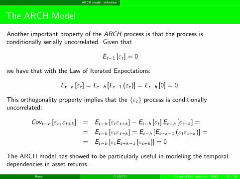
The ARCH Model

Another important property of the ARCH process is that the process isconditionally serially uncorrelated. Given that

Et−1 [εt ] = 0

we have that with the Law of Iterated Expectations:

Et−h [εt ] = Et−h [Et−1 (εt)] = Et−h [0] = 0.

This orthogonality property implies that the {εt} process is conditionallyuncorrelated:

Covt−h [εt , εt+k ] = Et−h [εtεt+k ]− Et−h [εt ]Et−h [εt+k ] =

= Et−h [εtεt+k ] = Et−h [Et+k−1 (εtεt+k)] =

= Et−h [εtEt+k−1 [εt+k ]] = 0

The ARCH model has showed to be particularly useful in modeling the temporaldependencies in asset returns.



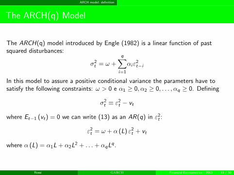
The ARCH(q) Model

The ARCH(q) model introduced by Engle (1982) is a linear function of pastsquared disturbances:

σ2t = ω +

q∑i=1

αiε2t−i

In this model to assure a positive conditional variance the parameters have tosatisfy the following constraints: ω > 0 e α1 ≥ 0, α2 ≥ 0, . . . , αq ≥ 0. Defining

σ2t ≡ ε2

t − vt

where Et−1 (vt) = 0 we can write (13) as an AR(q) in ε2t :

ε2t = ω + α (L) ε2

t + vt

where α (L) = α1L + α2L2 + . . .+ αqL

q.



The ARCH(q) Model

(1− α(L))ε2t = ω + vt

The process is weakly stationary if and only ifq∑

i=1

αi < 1; in this case the

unconditional variance is given by

E(ε2t

)= ω/ (1− α1 − . . .− αq) .



The ARCH(q) Model

The process is characterized by leptokurtosis in excess with respect to the normaldistribution. In the case, for example, of ARCH(1) with εt |Φt−1 ∼ N

(0, σ2

t

), the

kurtosis is equal to:

E(ε4t

)/E(ε2t

)2= 3

(1− α2

1

)/(1− 3α2

1

)with 3α2

1 < 1, when 3α21 = 1 we have

E(ε4t

)/E(ε2t

)2=∞.

In both cases we obtain a kurtosis coefficient greater than 3, characteristic of thenormal distribution.



The ARCH Regression Model

We have an ARCH regression model when the disturbances in a linear regressionmodel follow an ARCH process:

yt = x ′tb + εt

Et−1 (εt) = 0

εt |Φt−1 ∼ N(0, σ2

t

)Et−1

(ε2t

)≡ σ2

t = ω + α (L) ε2t


GARCH model

The GARCH(p,q) model

In order to model in a parsimonious way the conditional heteroskedasticity,Bollerslev (1986) proposed the Generalised ARCH model, i.e GARCH(p,q):

σ2t = ω + α (L) ε2

t + β (L)σ2t .

where α (L) = α1L + . . .+ αqLq, β (L) = β1L + . . .+ βpL

p.

The GARCH(1,1) is the most popular model in the empirical literature:

σ2t = ω + α1ε

2t−1 + β1σ

2t−1.


GARCH model


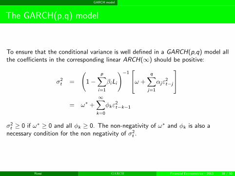
To ensure that the conditional variance is well defined in a GARCH(p,q) model allthe coefficients in the corresponding linear ARCH(∞) should be positive:

σ2t =

(1−

p∑i=1

βiLi

)−1ω +

q∑j=1

αjε2t−j

= ω∗ +

∞∑k=0

φkε2t−k−1

σ2t ≥ 0 if ω∗ ≥ 0 and all φk ≥ 0. The non-negativity of ω∗ and φk is also a

necessary condition for the non negativity of σ2t .


GARCH model


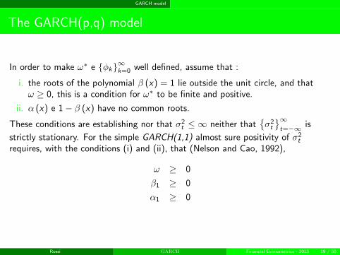
In order to make ω∗ e {φk}∞k=0 well defined, assume that :

i. the roots of the polynomial β (x) = 1 lie outside the unit circle, and thatω ≥ 0, this is a condition for ω∗ to be finite and positive.

ii. α (x) e 1− β (x) have no common roots.

These conditions are establishing nor that σ2t ≤ ∞ neither that

{σ2t

}∞t=−∞ is

strictly stationary. For the simple GARCH(1,1) almost sure positivity of σ2t

requires, with the conditions (i) and (ii), that (Nelson and Cao, 1992),

ω ≥ 0

β1 ≥ 0

α1 ≥ 0


GARCH model


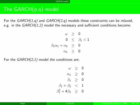
For the GARCH(1,q) and GARCH(2,q) models these constraints can be relaxed,e.g. in the GARCH(1,2) model the necessary and sufficient conditions become:

ω ≥ 0

0 ≤ β1 < 1

β1α1 + α2 ≥ 0

α1 ≥ 0

For the GARCH(2,1) model the conditions are:

ω ≥ 0

α1 ≥ 0

β1 ≥ 0

β1 + β2 < 1

β21 + 4β2 ≥ 0


GARCH model


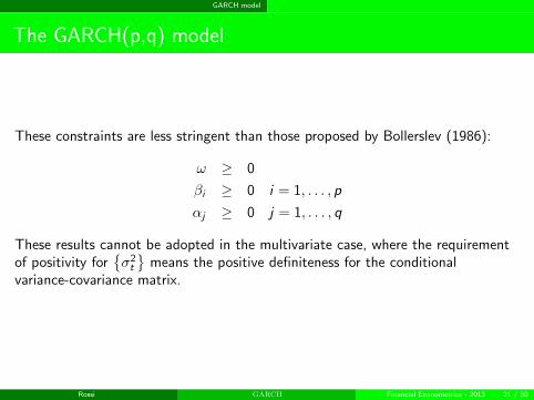
These constraints are less stringent than those proposed by Bollerslev (1986):

ω ≥ 0

βi ≥ 0 i = 1, . . . , p

αj ≥ 0 j = 1, . . . , q

These results cannot be adopted in the multivariate case, where the requirementof positivity for

{σ2t

}means the positive definiteness for the conditional

variance-covariance matrix.


GARCH model

Stationarity

The process {εt} which follows a GARCH(p,q) model is a martingale differencesequence. In order to study second-order stationarity it’s sufficient to considerthat:

Var [εt ] = Var [Et−1 (εt)] + E [Vart−1 (εt)] = E[σ2t

]and show that is asymptotically constant in time (it does not depend upon time).

A process {εt} which satisfies a GARCH(p,q) model with positive coefficientω ≥ 0, αi ≥ 0 i = 1, . . . , q, βi ≥ 0 i = 1, . . . , p is covariance stationary if and onlyif:

α (1) + β(1) < 1

This is a sufficient but non necessary conditions for strict stationarity. BecauseARCH processes are thick tailed, the conditions for covariance stationarity areoften more stringent than the conditions for strict stationarity.


GARCH model

Strict Stationarity GARCH(1,1)

Nelson shows that when ω > 0, σ2t <∞ a.s. and

{εt , σ

2t

}is strictly stationary if

and only if E[ln(β1 + α1z

2t

)]< 0

E[ln(β1 + α1z

2t

)]≤ ln

[E(β1 + α1z

2t

)]= ln (α1 + β1)

when α1 + β1 = 1 the model is strictly stationary. E[ln(β1 + α1z

2t

)]< 0 is a

weaker requirement than α1 + β1 < 1.ExampleARCH(1), with α1 = 1, β1 = 0, zt ∼ N (0, 1)

E[ln(z2t

)]≤ ln

[E(z2t

)]= ln (1)

It’s strictly but not covariance stationary. The ARCH(q) is covariance stationary ifand only if the sum of the positive parameters is less than one.


GARCH model

Forecasting volatility

Forecasting with a GARCH(p,q) (Engle and Bollerslev 1986):

σ2t+k = ω +

q∑i=1

αiε2t+k−i +

p∑i=1

βiσ2t+k−i

we can write the process in two parts, before and after time t:

σ2t+k = ω +

n∑i=1

[αiε

2t+k−i + βiσ

2t+k−i

]+

m∑i=k

[αiε

2t+k−i + βiσ

2t+k−i

]where n = min {m, k − 1} and by definition summation from 1 to 0 and fromk > m to m both are equal to zero. Thus

Et

[σ2t+k

]= ω +

n∑i=1

[(αi + βi )Et

(σ2t+k−i

)]+

m∑i=k

[αiε

2t+k−i + βiσ

2t+k−i

].


GARCH model

In particular for a GARCH(1,1) and k > 2:

Et

[σ2t+k

]=

k−2∑i=0

(α1 + β1)i ω + (α1 + β1)k−1σ2t+1

= ω

[1− (α1 + β1)k−1

][1− (α1 + β1)]

+ (α1 + β1)k−1σ2t+1

= σ2[1− (α1 + β1)k−1

]+ (α1 + β1)k−1

σ2t+1

= σ2 + (α1 + β1)k−1 [σ2t+1 − σ2

]When the process is covariance stationary, it follows that Et

[σ2t+k

]converges to

σ2 as k →∞.


GARCH model

The IGARCH(p,q) model

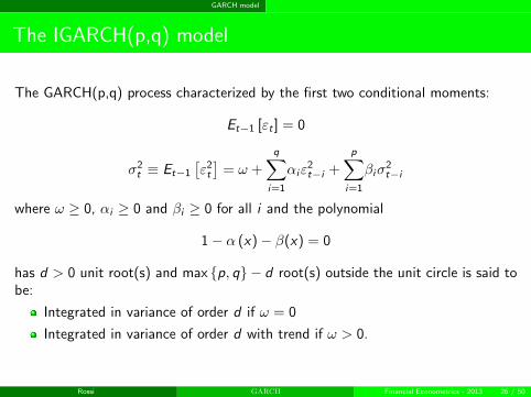
The GARCH(p,q) process characterized by the first two conditional moments:

Et−1 [εt ] = 0

σ2t ≡ Et−1

[ε2t

]= ω +

q∑i=1

αiε2t−i +

p∑i=1

βiσ2t−i

where ω ≥ 0, αi ≥ 0 and βi ≥ 0 for all i and the polynomial

1− α (x)− β(x) = 0

has d > 0 unit root(s) and max {p, q} − d root(s) outside the unit circle is said tobe:

Integrated in variance of order d if ω = 0

Integrated in variance of order d with trend if ω > 0.


GARCH model


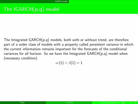
The Integrated GARCH(p,q) models, both with or without trend, are thereforepart of a wider class of models with a property called persistent variance in whichthe current information remains important for the forecasts of the conditionalvariances for all horizon. So we have the Integrated GARCH(p,q) model when(necessary condition)

α (1) + β(1) = 1


GARCH model


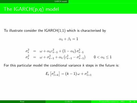
To illustrate consider the IGARCH(1,1) which is characterised by

α1 + β1 = 1

σ2t = ω + α1ε

2t−1 + (1− α1)σ2

t−1

σ2t = ω + σ2

t−1 + α1

(ε2t−1 − σ2

t−1

)0 < α1 ≤ 1

For this particular model the conditional variance k steps in the future is:

Et

[σ2t+k

]= (k − 1)ω + σ2

t+1


EGARCH

The EGARCH(p,q) Model

GARCH models assume that only the magnitude and not the positivity ornegativity of unanticipated excess returns determines feature σ2

t .

There exists a negative correlation between stock returns and changes inreturns volatility, i.e. volatility tends to rise in response to ”bad news”,(excess returns lower than expected) and to fall in response to ”good news”(excess returns higher than expected).


EGARCH


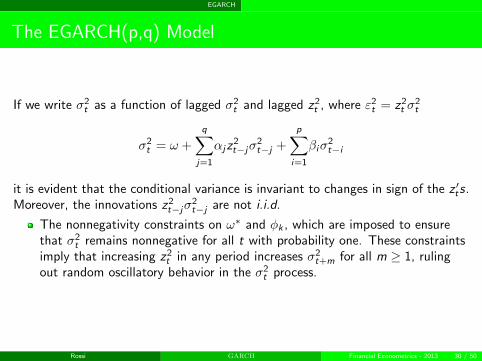
If we write σ2t as a function of lagged σ2

t and lagged z2t , where ε2

t = z2t σ

2t

σ2t = ω +

q∑j=1

αjz2t−jσ

2t−j +

p∑i=1

βiσ2t−i

it is evident that the conditional variance is invariant to changes in sign of the z ′ts.Moreover, the innovations z2

t−jσ2t−j are not i.i.d.

The nonnegativity constraints on ω∗ and φk , which are imposed to ensurethat σ2

t remains nonnegative for all t with probability one. These constraintsimply that increasing z2

t in any period increases σ2t+m for all m ≥ 1, ruling

out random oscillatory behavior in the σ2t process.


EGARCH


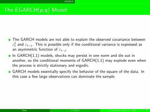
The GARCH models are not able to explain the observed covariance betweenε2t and εt−j . This is possible only if the conditional variance is expressed as

an asymmetric function of εt−j .

In GARCH(1,1) models, shocks may persist in one norm and die out inanother, so the conditional moments of GARCH(1,1) may explode even whenthe process is strictly stationary and ergodic.

GARCH models essentially specify the behavior of the square of the data. Inthis case a few large observations can dominate the sample.


EGARCH


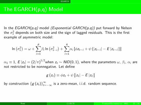
In the EGARCH(p,q) model (Exponential GARCH(p,q)) put forward by Nelsonthe σ2

t depends on both size and the sign of lagged residuals. This is the firstexample of asymmetric model:

ln(σ2t

)= ω +

p∑i=1

βi ln(σ2t−i)

+

q∑i=1

αi [φzt−i + ψ (|zt−i | − E |zt−i |)]

α1 ≡ 1, E |zt | = (2/π)1/2when zt ∼ NID(0, 1), where the parameters ω, βi , αi arenot restricted to be nonnegative. Let define

g (zt) ≡ φzt + ψ [|zt | − E |zt |]

by construction {g (zt)}∞t=−∞ is a zero-mean, i.i.d. random sequence.


EGARCH


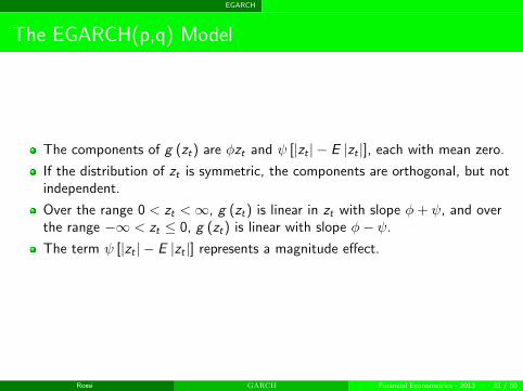
The components of g (zt) are φzt and ψ [|zt | − E |zt |], each with mean zero.

If the distribution of zt is symmetric, the components are orthogonal, but notindependent.

Over the range 0 < zt <∞, g (zt) is linear in zt with slope φ+ ψ, and overthe range −∞ < zt ≤ 0, g (zt) is linear with slope φ− ψ.

The term ψ [|zt | − E |zt |] represents a magnitude effect.


EGARCH


If ψ > 0 and φ = 0, the innovation in ln(σ2t+1

)is positive (negative) when

the magnitude of zt is larger (smaller) than its expected value.

If ψ = 0 and φ < 0, the innovation in conditional variance is now positive(negative) when returns innovations are negative (positive).

A negative shock to the returns which would increase the debt to equity ratioand therefore increase uncertainty of future returns could be accounted forwhen αi > 0 and φ < 0.


EGARCH


Nelson assumes that zt has a GED distribution (exponential power family). Thedensity of a GED random variable normalized is:

f (z ; υ) =υ exp

[−(

12

)|z/λ|υ

]λ2(1+1/υ)Γ (1/υ)

−∞ < z <∞, 0 < υ ≤ ∞


EGARCH


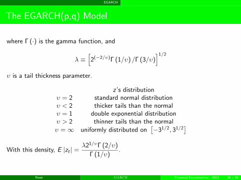
where Γ (·) is the gamma function, and

λ ≡[2(−2/υ)Γ (1/υ) /Γ (3/υ)

]1/2

υ is a tail thickness parameter.

z ’s distributionυ = 2 standard normal distributionυ < 2 thicker tails than the normalυ = 1 double exponential distributionυ > 2 thinner tails than the normalυ =∞ uniformly distributed on

[−31/2, 31/2

]With this density, E |zt | =

λ21/υΓ (2/υ)

Γ (1/υ).


Asymmetric Models

Non linear ARCH(p,q) Model

The Non linear ARCH(p,q) model (Engle - Bollerslev 1986):

σγt = ω +

q∑i=1

αi |εt−i |γ +

p∑i=1

βiσγt−i

σγt = ω +

q∑i=1

αi |εt−i − k |γ +

p∑i=1

βiσγt−i

for k 6= 0, the innovations in σγt will depend on the size as well as the sign oflagged residuals, thereby allowing for the leverage effect in stock return volatility.


Asymmetric Models

GJR model

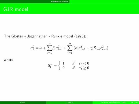
The Glosten - Jagannathan - Runkle model (1993):

σ2t = ω +

p∑i=1

βiσ2t−i +

q∑i=1

(αiε

2t−1 + γiS

−t−iε

2t−i)

where

S−t =

{1 if εt < 00 if εt ≥ 0


Asymmetric Models

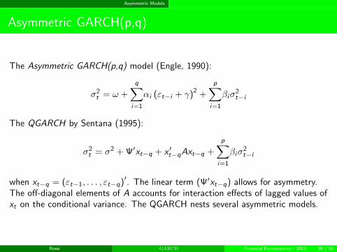
Asymmetric GARCH(p,q)

The Asymmetric GARCH(p,q) model (Engle, 1990):

σ2t = ω +

q∑i=1

αi (εt−i + γ)2 +

p∑i=1

βiσ2t−i

The QGARCH by Sentana (1995):

σ2t = σ2 + Ψ′xt−q + x ′t−qAxt−q +

p∑i=1

βiσ2t−i

when xt−q = (εt−1, . . . , εt−q)′. The linear term (Ψ′xt−q) allows for asymmetry.The off-diagonal elements of A accounts for interaction effects of lagged values ofxt on the conditional variance. The QGARCH nests several asymmetric models.


Asymmetric Models

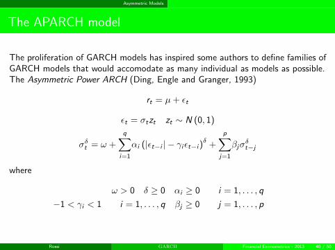
The APARCH model

The proliferation of GARCH models has inspired some authors to define families ofGARCH models that would accomodate as many individual as models as possible.The Asymmetric Power ARCH (Ding, Engle and Granger, 1993)

rt = µ+ εt

εt = σtzt zt ∼ N (0, 1)

σδt = ω +

q∑i=1

αi (|εt−i | − γiεt−i )δ +

p∑j=1

βjσδt−j

where

ω > 0 δ ≥ 0 αi ≥ 0 i = 1, . . . , q

−1 < γi < 1 i = 1, . . . , q βj ≥ 0 j = 1, . . . , p


Asymmetric Models

The APARCH model

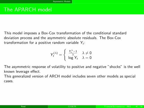
This model imposes a Box-Cox transformation of the conditional standarddeviation process and the asymmetric absolute residuals. The Box-Coxtransformation for a positive random variable Yt :

Y(λ)t =

{Yλt −1λ λ 6= 0

logYt λ = 0

The asymmetric response of volatility to positive and negative ”shocks” is the wellknown leverage effect.This generalized version of ARCH model includes seven other models as specialcases.


Asymmetric Models

The APARCH model

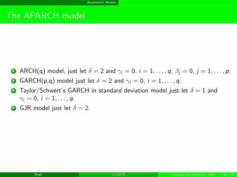
1 ARCH(q) model, just let δ = 2 and γi = 0, i = 1, . . . , q, βj = 0, j = 1, . . . , p.

2 GARCH(p,q) model just let δ = 2 and γi = 0, i = 1, . . . , q.

3 Taylor/Schwert’s GARCH in standard deviation model just let δ = 1 andγi = 0, i = 1, . . . , q.

4 GJR model just let δ = 2.


GARCH-in-mean model

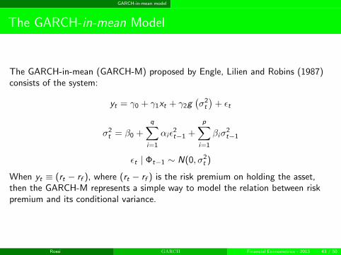
The GARCH-in-mean Model

The GARCH-in-mean (GARCH-M) proposed by Engle, Lilien and Robins (1987)consists of the system:

yt = γ0 + γ1xt + γ2g(σ2t

)+ εt

σ2t = β0 +

q∑i=1

αiε2t−1 +

p∑i=1

βiσ2t−1

εt | Φt−1 ∼ N(0, σ2t )

When yt ≡ (rt − rf ), where (rt − rf ) is the risk premium on holding the asset,then the GARCH-M represents a simple way to model the relation between riskpremium and its conditional variance.


GARCH-in-mean model

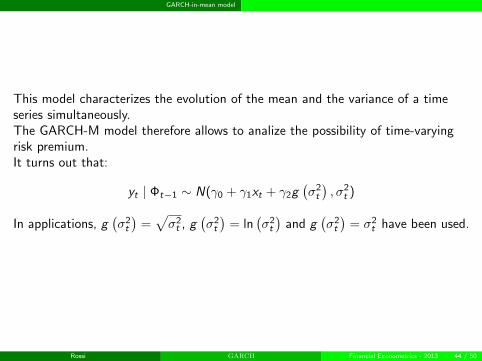
This model characterizes the evolution of the mean and the variance of a timeseries simultaneously.The GARCH-M model therefore allows to analize the possibility of time-varyingrisk premium.It turns out that:

yt | Φt−1 ∼ N(γ0 + γ1xt + γ2g(σ2t

), σ2

t )

In applications, g(σ2t

)=√σ2t , g

(σ2t

)= ln

(σ2t

)and g

(σ2t

)= σ2

t have been used.


The News Impact Curve


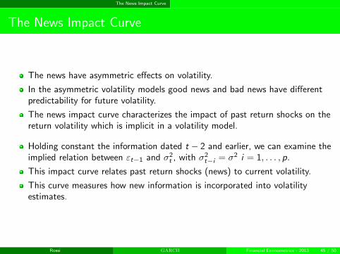
The news have asymmetric effects on volatility.

In the asymmetric volatility models good news and bad news have differentpredictability for future volatility.

The news impact curve characterizes the impact of past return shocks on thereturn volatility which is implicit in a volatility model.

Holding constant the information dated t − 2 and earlier, we can examine theimplied relation between εt−1 and σ2

t , with σ2t−i = σ2 i = 1, . . . , p.

This impact curve relates past return shocks (news) to current volatility.

This curve measures how new information is incorporated into volatilityestimates.



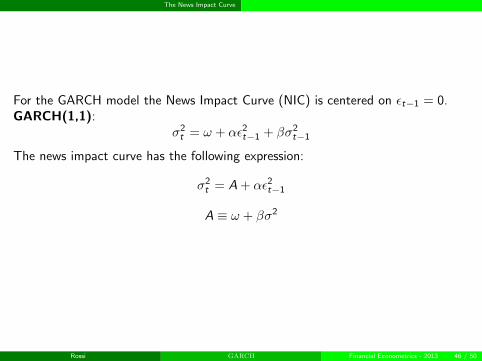
For the GARCH model the News Impact Curve (NIC) is centered on εt−1 = 0.GARCH(1,1):

σ2t = ω + αε2

t−1 + βσ2t−1

The news impact curve has the following expression:

σ2t = A + αε2

t−1

A ≡ ω + βσ2



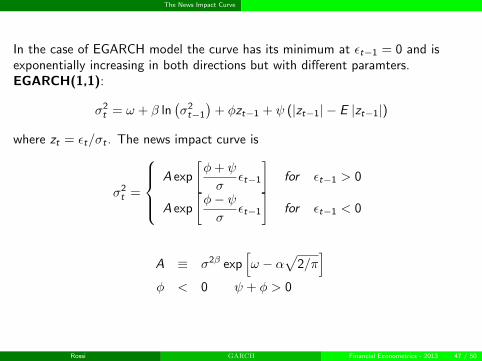
In the case of EGARCH model the curve has its minimum at εt−1 = 0 and isexponentially increasing in both directions but with different paramters.EGARCH(1,1):

σ2t = ω + β ln

(σ2t−1

)+ φzt−1 + ψ (|zt−1| − E |zt−1|)

where zt = εt/σt . The news impact curve is

σ2t =

A exp

[φ+ ψ

σεt−1

]for εt−1 > 0

A exp

[φ− ψσ

εt−1

]for εt−1 < 0

A ≡ σ2β exp[ω − α

√2/π

]φ < 0 ψ + φ > 0



The EGARCH allows good news and bad news to have different impact onvolatility, while the standard GARCH does not.

The EGARCH model allows big news to have a greater impact on volatilitythan GARCH model. EGARCH would have higher variances in both directionsbecause the exponential curve eventually dominates the quadrature.



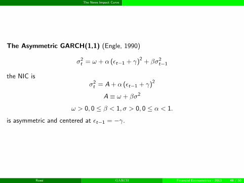
The Asymmetric GARCH(1,1) (Engle, 1990)

σ2t = ω + α (εt−1 + γ)2 + βσ2

t−1

the NIC isσ2t = A + α (εt−1 + γ)2

A ≡ ω + βσ2

ω > 0, 0 ≤ β < 1, σ > 0, 0 ≤ α < 1.

is asymmetric and centered at εt−1 = −γ.



The Glosten-Jagannathan-Runkle model

σ2t = ω + αε2

t + βσ2t−1 + γS−t−1ε

2t−1

S−t−1 =

{1 if εt−1 < 0

0 otherwise

The NIC is

σ2t =

{A + αε2

t−1 if εt−1 > 0A + (α + γ) ε2

t−1 if εt−1 < 0

A ≡ ω + βσ2

ω > 0, 0 ≤ β < 1, σ > 0, 0 ≤ α < 1, α + β < 1

is centered at εt−1 = −γ.


Documents

GARCH Models - unipveconomia.unipv.it/pagp/pagine_personali/.../Rossi_GARCH_Ec_Fin_20… · Stylized Facts Stylized Facts GARCH models have been developed to account for empirical