STYLIZED FACTS AND DYNAMIC MODELING OF HIGH-FREQUENCY DATA ON PRECIOUS METALS

MASSIMILIANO CAPORIN ANGELO RANALDO GABRIEL G. VELO WORKING PAPERS ON FINANCE NO. 2013/18 SWISS INSTITUTE OF BANKING AND FINANCE (S/BF – HSG)

MAY 2013

Electronic copy available at: http://ssrn.com/abstract=2263927

Stylized facts and dynamic modeling of high-frequency

data on precious metals

Massimiliano Caporin∗ Angelo Ranaldo† Gabriel G. Velo‡

May 8, 2013

Abstract: Taking advantage of a trades-and-quotes database, the main stylized factsand dynamic properties of a time series related to spot precious metals, that is, gold,silver, palladium, and platinum, are documented. The behavior of spot prices, returns,volume, and selected liquidity measures is analyzed. A clear evidence of periodic patternsmatching the trading hours of the most active markets, London, Zurich, New York, as wellas Asian markets, is found. The time series of spot returns have thus properties similarto those of traditional financial assets with fat tails, asymmetry, periodic behaviors in theconditional variances, and volatility clustering. The empirical analyzes show, as expected,that gold is the most liquid and less volatile asset, whereas palladium and platinum aretraded less.Keywords: precious metals, high-frequency data, liquidity measurement, intradaily pe-riodicity.JEL Classifications: C58, C22, C52, G10.

∗Department of Economics and Management Marco Fanno, University of Padova; correspondingauthor: Via del Santo 22, Padova, Italy, Tel: +39 049/8274258. Fax: +39 049/8274211. Email:massimiliano.caporin@unipd.it.

†University of St. Gallen, Swiss Institute of Banking and Finance, Rosenbergstrasse 52, St.Gallen,Switerland, angelo.ranaldo@unisg.ch.

‡Department of Economics and Management Marco Fanno, University of Padova, Via del Santo 22,Padova, Italy,gabriel.velo@unipd.it.

1

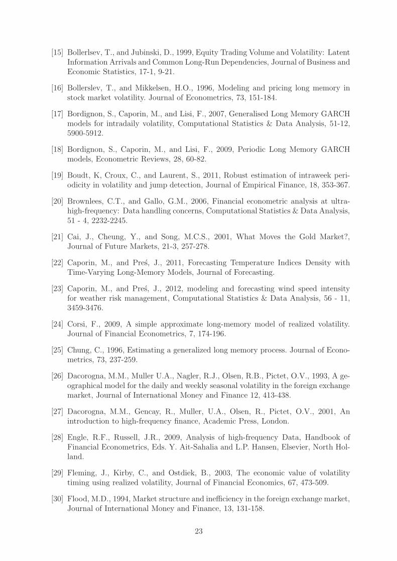
Electronic copy available at: http://ssrn.com/abstract=2263927

1 Introduction

In the last twenty years there has been a growing interest in high-frequency data. Ac-cess to these data sources leads to the development of studies and empirical research inseveral directions. From an economic point of view, research has focused on agent’s be-havior and market microstructure (price formation, asymmetric information, news andannouncement impact). Within a statistical or quantitative framework, different authorshave studied the features or stylized facts of high-frequency time series (prices, returns,volumes, liquidity, duration) and proposed appropriate modeling strategies. In the quan-titative investment field, the empirical research leads to the development of quantitativetrading rules. Finally, within a risk management perspective, we place the studies dealingwith the development of daily variance estimators by means of high-frequency returns.1

Interest in high-frequency data began with the pioneering work on data collected byOlsen Associates (see Dacorogna et al., 2001), which focused on currencies and were thenextended to other asset classes. With the development of IT tools, the high-frequencyfinance literature also gained access to book data, with further developments from boththe theoretical and empirical points of view (see Parlour and Seppi, 2008).

However, only a few authors have discussed the properties of high-frequency data onprecious metals. Cai et al. (2001) focus on 5-minute gold future returns. They study theperiodicity in absolute returns and link its movements to macroeconomic announcements.Fleming et al. (2003) make use of realized volatility on several assets and determine theeconomic value of volatility timing. Their study includes 5-minute returns of gold futurescontracts. Baillie et al. (2007) analyze the dynamic behavior of several daily and 5-minutecommodity futures prices, including the gold future. Bannouh et al. (2009) work on co-range computation (an estimator of the integrated covariance) with a trade dataset thatincludes the gold future. Finally, Khalifa et al. (2011) focus on volatility measurementand forecasting of several commodity future prices, including gold and silver. All of theaforementioned studies have a common element: They work on New York futures data.Moreover, to the best of our knowledge, gold has piqued the greatest amount of interest,whereas silver has only attracted limited attention. We support this by the larger amountof interest in gold, compared with other precious metals, and the perception of gold as asafe-haven investment.

Our work belongs to the strand of literature focusing on high-frequency data on pre-cious metals. We differ from previous studies in many respects because of our uniquedatabase. First, we have access to high-frequency data about four different precious met-als: gold, silver, palladium, and platinum. Second, our data are related to spot pricesand not futures contracts. Therefore, the time-series behaviors might be different as aconsequence of the different uses associated with spot and future contracts. To our knowl-edge, there is no literature on palladium, and platinum high-frequency data. Third, wehave access to a brokerage house database that operates on a 24-hours basis. As a result,the movement we observe in high-frequency time series can be linked to the activity indifferent precious metals markets, including New York but also the European markets(London and Zurich) and the Asian markets. This is of relevant interest because previous

1Several references to the previous topics can be found in O’Hara (1997), Bauwens and Giot (2001),Dacorogna et al. (2001), Hasbrouck (2007), Engle and Russell (2009), Hautsch (2011), Schmidt (2011),Ye (2011), and Abergel et al. (2012), among others.

1

works only focused on a specific market. Fourth, we differ from previous works becauseof our access to a trade-and-quotes dataset. From the trade side, we have trade prices,associated volumes, and order side (allowing us to precisely distinguish seller-initiatedfrom buyer-initiated orders). On the quote side of the database, we have access to thelimited order book up to ten levels, with prices and volumes, which makes feasible theevaluation of liquidity and market depth. Finally, the time frequency of the databaseis extremely high, with book updates reaching a 100-millisecond frequency. Because ofthe novelty of our database, the pure statistical analysis of high-frequency spot data onprecious metals is per se interesting and relevant.

In this work, we focus on the stylized facts and dynamic properties of the preciousmetals data. We start from the most traditional time series, prices, and returns, andthen focus on the volatility, preliminary measured from squared returns and then filteredwith periodic components and GARCH-type models. We move later to volume time se-ries and to two specific liquidity measures, the order flow, and the percentage quotedspread. These two quantities provide a first look at the information one might extractfrom a trade-and-quotes database on precious metals. The analyses reported here are,by construction, preliminary to further economic applications at both the univariate andmultivariate level. Later studies will take advantage of the findings in the current paper.There are several areas in which our results might be useful: (1) in trading, because thedynamic properties we identify and the models we propose might be used to produceforecasts of prices and volumes, with potential extensions that include trade durationand liquidity as further covariates;, (2) in risk management, as we provide some evidenceon the volatility behavior and on its modeling, (3) in event studies, where the dynamicbehavior of prices, returns, volume and liquidity might be correlated to scheduled and/orunanticipated announcements, and (4) in studies dealing with safe-haven effects, in whichprecious metals may represent refuge assets.

The time-series analyzed here are characterized by the presence of a periodic behav-ior in their levels and/or in the second-order moment. Such a finding is expected as weconsider intradaily data. However, the periodic movement is associated with the tradingactivity of the main markets active in precious metals trading, which can be identified, forinstance, with peaks in the volatility of the returns time series. This result has relevantaffinities to the periodic behavior observed by Dacorogna et al. (1993) on the foreignexchange market. For each of the analyzed series, we suggest the use of a dynamic modelfor capturing the serial dependence in the mean and/or in the variance. The proposedspecifications seem appropriate in the whitening of the analyzed time series and allow thedevelopment of research based on time-series forecasting.

This paper proceeds as follows: Section 2 describes the dataset and the variables ofinterest; Section 3 focuses on the stylized facts of prices, returns, volumes, and liquiditytime series; Section 4 deals with dynamic models; and Section 5 concludes.

2

2 Database description, data handling, and the ana-

lyzed quantities

The database used in this study has been provided by ICAP through its EBS platform.EBS is the leading interdealer trading platform for currencies, and data provided by EBShave been already used in academic research (see, for instance, Berger et al., 2008 andMancini et al., 2012). The database we access is equivalent to that adopted in Mancini etal. (2012) and includes more than fifty currencies and four precious metals. For all assetsmade available, the trades and quotes refer to spot prices. In this work we focus on theprecious metals: gold (identified by the ticker XAU), silver (XAG), palladium (XPD), andplatinum (XPT). We consider spot prices against the U.S. dollar and refer to one ounce(for instance, gold quotes are U.S. dollar per one gold ounce). The data we analyze spanthe period beginning with December 27, 2008 to November 30, 2010. The dataset includesthe recorded trades coupled with the information on the active part of the contract, thetraded volume, and the trade price. The presence of the maker and taker sides opensthe door to the construction of the order flow. Notably, as observed by Mancini et al.(2012), trade direction data are known and do not need to be inferred by means of rulessuch as done by Lee and Ready (1991). Besides the trade data, the database includesthe binding tradable bid and ask quotes, together with the related volume. In this case,the information is provided for the book up to the tenth level. However, here we presentanalyses based on the trade data and on the best bid and ask quotes. Moreover, we dis-cuss the dynamic features of the data, comparing our findings to those of previous studies.

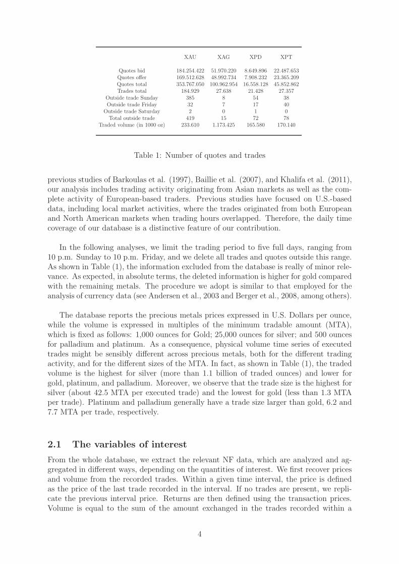
In the EBS database, data are recorded at a very high frequency (let us call themnanofrequency data, or NF data2). From December 27, 2008 to the end of August 2009,the observation frequency is 250 milliseconds; from the first of September 2009 to the endof the sample, the observation frequency increases to 100 milliseconds.3 As a result, newinformation is recorded by the system every 100/250 milliseconds if at least one of thefollowing events takes place: an order is executed and/or a new quote is entered/deletedand/or a new volume is entered into the system at a quote already present in the system.The last case produces a new flash of the book because each flash includes the numberof quotes in the market for each side/price together with the available volume. Table (1)reports the total number of trades (buyer/seller initiated) and quotes (by market side) byprecious metals that are included in the database. We note that gold is the metal withthe highest activity, both in terms of trades and quotes. Silver has less than one-third ofthe quotes of gold and is followed by platinum and then palladium. The last has less thana twentieth of gold quotes. Excluding gold, with about 185 thousand trades, the otherprecious metals have a similar number of trades.

Data are recorded on a GMT time scale, on a 24-hour basis, 7 days a week. As a result,there are quotes and trades executed from buyers/sellers located in different geographicalareas. To the best of our knowledge, this study provides for the first time an analysis onprecious metal trades jointly covering the most active world markets. Compared with the

2We thank Michael McAleer for suggesting the use of this name for our dataset.3The 100-millisecond frequency begins August 28, 2009, but a few days in July 2009, likely the

testing period, use the 100-millisecond frequency. Moreover, both frequencies (100 and 250 milliseconds)are present on July 21, 2009, and August 28, 2009. This finding does not affect our results because weaggregate data at lower frequencies.

3

XAU XAG XPD XPT

Quotes bid 184.254.422 51.970.220 8.649.896 22.487.653Quotes offer 169.512.628 48.992.734 7.908.232 23.365.209Quotes total 353.767.050 100.962.954 16.558.128 45.852.862Trades total 184.929 27.638 21.428 27.357

Outside trade Sunday 385 8 54 38Outside trade Friday 32 7 17 40

Outside trade Saturday 2 0 1 0Total outside trade 419 15 72 78

Traded volume (in 1000 oz) 233.610 1.173.425 165.580 170.140

Table 1: Number of quotes and trades

previous studies of Barkoulas et al. (1997), Baillie et al. (2007), and Khalifa et al. (2011),our analysis includes trading activity originating from Asian markets as well as the com-plete activity of European-based traders. Previous studies have focused on U.S.-baseddata, including local market activities, where the trades originated from both Europeanand North American markets when trading hours overlapped. Therefore, the daily timecoverage of our database is a distinctive feature of our contribution.

In the following analyses, we limit the trading period to five full days, ranging from10 p.m. Sunday to 10 p.m. Friday, and we delete all trades and quotes outside this range.As shown in Table (1), the information excluded from the database is really of minor rele-vance. As expected, in absolute terms, the deleted information is higher for gold comparedwith the remaining metals. The procedure we adopt is similar to that employed for theanalysis of currency data (see Andersen et al., 2003 and Berger et al., 2008, among others).

The database reports the precious metals prices expressed in U.S. Dollars per ounce,while the volume is expressed in multiples of the minimum tradable amount (MTA),which is fixed as follows: 1,000 ounces for Gold; 25,000 ounces for silver; and 500 ouncesfor palladium and platinum. As a consequence, physical volume time series of executedtrades might be sensibly different across precious metals, both for the different tradingactivity, and for the different sizes of the MTA. In fact, as shown in Table (1), the tradedvolume is the highest for silver (more than 1.1 billion of traded ounces) and lower forgold, platinum, and palladium. Moreover, we observe that the trade size is the highest forsilver (about 42.5 MTA per executed trade) and the lowest for gold (less than 1.3 MTAper trade). Platinum and palladium generally have a trade size larger than gold, 6.2 and7.7 MTA per trade, respectively.

2.1 The variables of interest

From the whole database, we extract the relevant NF data, which are analyzed and ag-gregated in different ways, depending on the quantities of interest. We first recover pricesand volume from the recorded trades. Within a given time interval, the price is definedas the price of the last trade recorded in the interval. If no trades are present, we repli-cate the previous interval price. Returns are then defined using the transaction prices.Volume is equal to the sum of the amount exchanged in the trades recorded within a

4

given time interval, regardless of the trade side (buyer/seller initiated). If a given timeinterval does not include trades, the volume is equal to zero. In the following, we denotethe daily time index by t, the intradaily period by i = 1, 2, . . .N with N denoting thenumber of intradaily periods in day t. Intradaily periods have length equal to 1/N days,or 1440/N minutes. Furthermore, we indicate the end of period i of day t as (i, t), andwe use the following notation. The intradaily price sequence is denoted by pi,t, whilethe intradaily volume time series is given as vi,t; the intradaily log-returns are defined asri,t = log (pi,t)− log (pi−1,t) , i = 2, 3, . . .N , and r1,t = log (p1,t)− log (pN,t−1).

4

Finally, we filter quote data from outliers, most likely associated to errors in matchingthe asset identifier and the price.5 We choose a simple approach, excluding all quotes witha value 20% higher (for buyer initiated) or lower (for seller initiated) than the averagetrade price of the day.

The financial economics and econometrics literature includes several liquidity measures(see the survey by Gabrielsen et al., 2011). In this study, we focus on specific quantitiesthat are exploiting part of the informative content of the database. We restrict ourattention to the order flow, OFi,t, and to the percentage quoted spread, QSi,t, defined asfollows.

• Order flow: Let h denote the execution time of an order, and denote by xh the tradedirection of the order recorded at time h; the trade direction is equal to −1 forseller-initiated trades and +1 for buyer-initiated trades; the order flow for interval iof day t is equal to OFi,t =

∑

(i−1,t)<j≤(i,t) xh; by definition, the order flow assumes

only integer values and can be either positive or negative.6

• Percentage quoted spread: Let Ai,t and Bi,t denote the best ask and bid Pricesavailable in the book at the end of period i at day t; we define the midquote asMi,t = 0.5 (Ai,t +Bi,t) and the percentage quoted spread as QSi,t =

Ai,t−Bi,t

Mi,t.

The percentage quoted spread we consider is a standardized quantity allowing a directcomparison across precious metals because it is not dependent on the price of the MTA.

We study time series of the previously defined quantities at different frequencies. Weanalyze returns and volumes at the 5- and 60-minutes frequencies, where the first caseis only considered for gold and silver, due to the higher number of trades recorded forthese two metals. We inspect liquidity measures at the 15- and 60-minutes frequencies.When the frequency is set at 60 minutes, the dataset contains 11,880 observations. Thenumber increases to 47,520 when considering the 15-minutes frequency and to 142,560at the 5-minute frequency. We do not consider higher frequencies because of the largenumber of zeros that would be observed in the time series of interest (see the following

4When computing the first return of the week on Sunday evening, we compute the returns withrespect to the last price observed on Friday evening. In addition, we have only removed a few bankholidays (New Year’s Day [2009 and 2010], Good Friday [2009 and 2010], and Christmas Day [2009]).Two days are not included in the database because of missing data: They are May 17, 2010, and May18, 2010 (a Monday and a Tuesday).

5See, for example, Brownlees and Gallo (2006) for high-frequency data-cleaning techniques.6Note that different orders (at different prices) might be recorded at the same time; these must all

be considered in the construction of the order flow.

5

section for further details).

3 Stylized facts of precious metals price, return, vol-

ume, and liquidity

In this section, we focus on those features that characterize the time series of returns,volume, and liquidity of our four precious metals. In particular, we evaluate the serialcorrelation properties of the first- and second-order moments, the distribution, and theexistence of periodic patterns.

3.1 Prices and returns

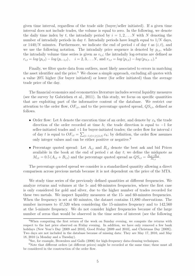
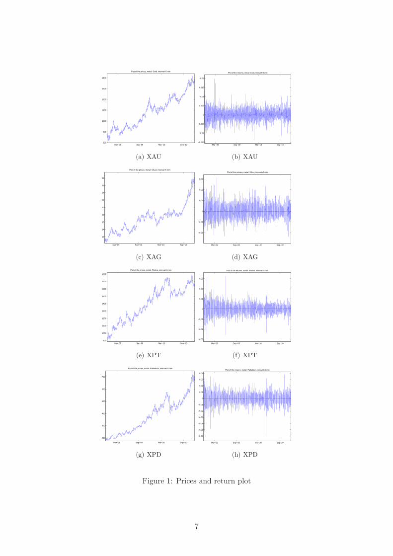
The prices of precious metals follow an upward-sloping behavior in the analyzed sample(see Figure (1)). This might depend on the so-called safe-haven effect, that is, the out-flow from risky financial assets toward the precious metals, which are perceived as saferinvestments during periods of high uncertainty. We first analyze the series to determinetheir integration properties. ADF tests confirm that the log-prices follow a Random Walkmodel and suggest focusing on returns time series.7

Returns time series have patterns similar to those of equity returns and are charac-terized by volatility clustering, as well as the presence of extreme movements (see Figure(1)). The descriptive analysis, reported in Table (2), suggests that gold returns are lessvolatile than other precious metals, at both the 5- and 60-minutes frequencies. This find-ing is also matched with an inverse relation in average returns, the lowest being that ofgold. We support that by the larger interest for gold compared with silver, platinum,and palladium, which might lead to higher efficiency for this precious metal. In turn,this leads to smaller risk and lower returns. The kurtosis is similar across metals at thehourly frequency, whereas at the 5-minute level, gold has a much smaller kurtosis thansilver. Nevertheless, as we discuss in the following paragraph, this might be influenced bythe large amount of zeros in the silver time series. Finally, we observe that the skewnessis negative for silver, palladium, and platinum at the 60-minute frequency, a behaviorsimilar to that observed in equities. However, gold returns have positive skewness. Con-sidering the range analyzed in this paper, 2009 and 2010, the trend of price time series,and the considerable interest in gold, this result is unsurprising. It suggests that, in theconsidered period, trades on gold led to a consistent increase in the price of gold over time.When focusing on the returns ACF, we have statistically significant positive correlationsfor the first lag at the 5-minute level, whereas at the 60-minutes frequency, the first ACFbecomes negative but is still statistically significant. The presence of negative correlationis expected on high-frequency data and might have different explanations: bid-ask bounce(Bollerslev and Bomowitz, 1993), order imbalance (Flood, 1994), and/or trade behavior(Engle and Russell, 2009, among others). Such serial correlation has to be taken intoaccount when developing models for the returns time series.

Regarding the trade activity, the proportion of zeros in a given interval of time canbe seen as a measure of market liquidity (or illiquidity). For example, Bekaert et al.

7ADF tests are available upon request.

6

Mar−09 Sep−09 Mar−10 Sep−10800

900

1000

1100

1200

1300

1400

Plot of the prices, metal: Gold, interval=5 min

(a) XAU

Mar−09 Sep−09 Mar−10 Sep−10−0.015

−0.01

−0.005

0

0.005

0.01

0.015

0.02

Plot of the returns, metal: Gold, interval=5 min

(b) XAU

Mar−09 Sep−09 Mar−10 Sep−10

12

14

16

18

20

22

24

26

28

Plot of the prices, metal: Silver, interval=5 min

(c) XAG

Mar−09 Sep−09 Mar−10 Sep−10

−0.02

−0.01

0

0.01

0.02

0.03

Plot of the returns, metal: Silver, interval=5 min

(d) XAG

Mar−09 Sep−09 Mar−10 Sep−10900

1000

1100

1200

1300

1400

1500

1600

1700

1800

Plot of the prices, metal: Platino, interval=5 min

(e) XPT

Mar−09 Sep−09 Mar−10 Sep−10

−0.03

−0.02

−0.01

0

0.01

0.02

0.03

Plot of the returns, metal: Platino, interval=5 min

(f) XPT

Mar−09 Sep−09 Mar−10 Sep−10

200

300

400

500

600

700

Plot of the prices, metal: Palladium, interval=5 min

(g) XPD

Mar−09 Sep−09 Mar−10 Sep−10

−0.06

−0.05

−0.04

−0.03

−0.02

−0.01

0

0.01

0.02

0.03

0.04

Plot of the returns, metal: Palladium, interval=5 min

(h) XPD

Figure 1: Prices and return plot

7

Return Volume

XAU XAU XAG XAG XPD XPT XAU XAU XAG XAG XPD XPTFrequency 5 60 5 60 60 60 5 60 5 60 60 60Mean 0.0003 0.0038 0.0006 0.0079 0.0115 0.0049 1.6387 19.664 8.2311 98.773 13.937 14.321Median 0.0000 0.0000 0.0000 0.0000 0.0000 0.0000 0.0000 12 0.0000 25 0.0000 5Std 0.0763 0.2582 0.1240 0.4499 0.5205 0.3369 3.5198 25.574 30.515 173.15 30.221 24.502

Kurtosis 30.09 15.643 62.863 15.361 17.266 10.577 51.952 18.375 100.90 22.274 41.431 30.443Skewness 0.1031 0.3347 0.5407 −0.059 −0.569 −0.305 5.2819 3.0949 7.3061 3.5571 4.9074 3.92875% quant. −0.104 −0.385 −0.039 −0.701 −0.795 −0.540 0.0000 0.0000 0.0000 0.0000 0.0000 0.000050% quant. 0.0000 0.0000 0.0000 0.0000 0.0000 0.0000 0.0000 12 0.0000 25 0.0000 595% quant. 0.1070 0.3841 0.0545 0.7305 0.8564 0.5458 8 68 50 450 65 60n. of 0 83592 1772 126534 5513 7063 5572 79842 1580 125250 5268 6354 5087

Table 2: Descriptive analysis: Returns and Volume across metals

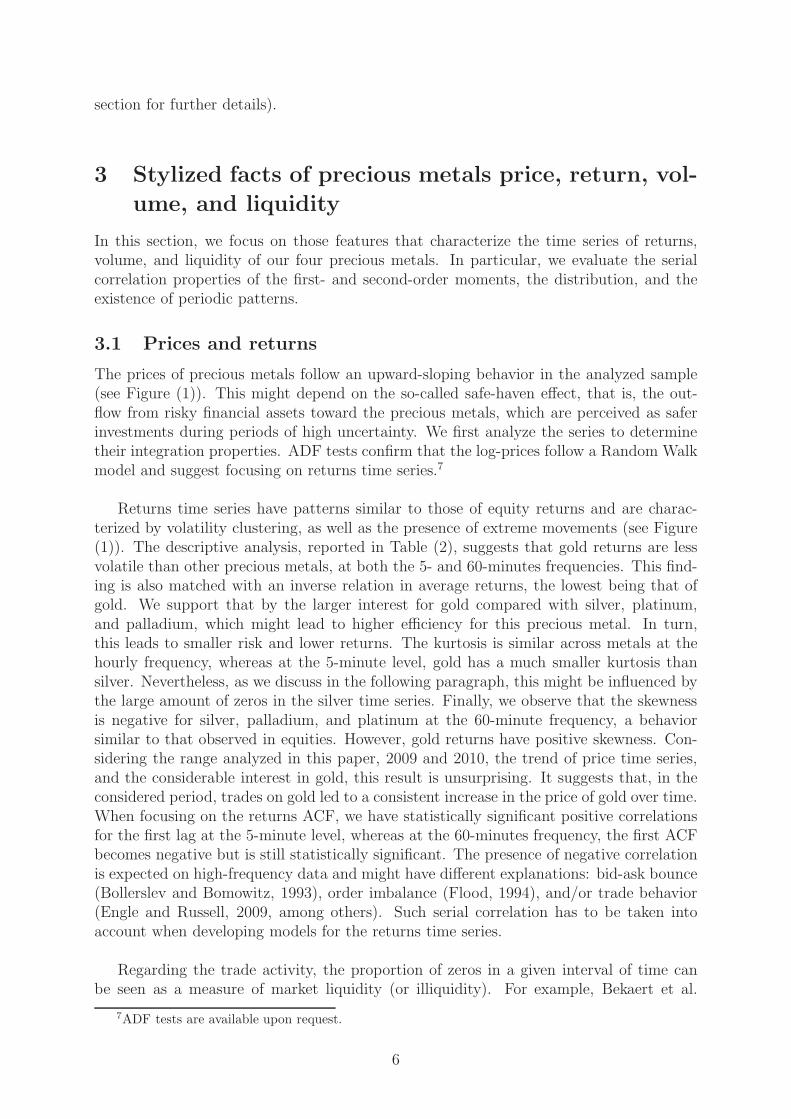
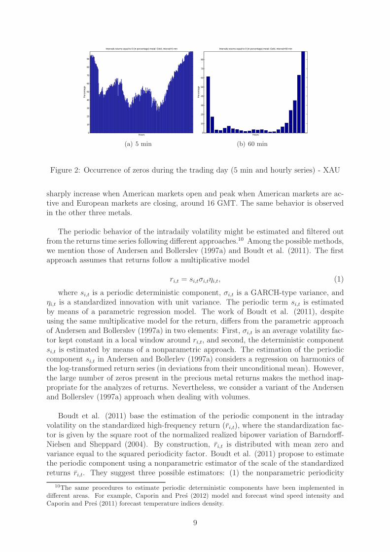
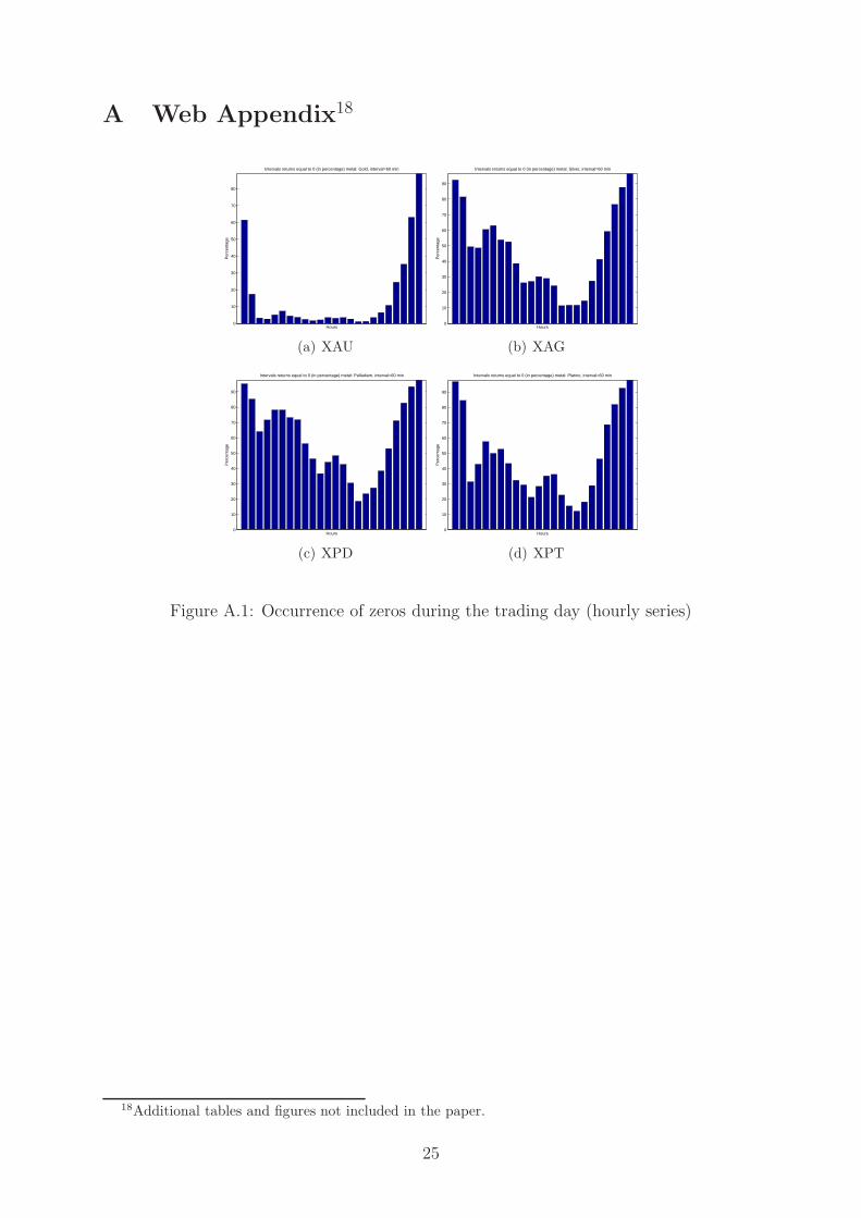
(2007) examine the impact of liquidity, proxied by the proportion of zero daily firm re-turns averaged over the month in emerging equity markets, on expected returns. Table(2) highlights that the number of zero returns is sensibly high. The percentage of ze-ros on hourly data is close to 45% for silver and platinum, peaks at 60% for palladium,and is minimum, about 15%, for gold. We report 5-minute descriptive statistics for goldand silver, the two most traded metals, showing that the number of zeros increases to60% for gold and 90% for silver. The existence of such a large number of zeros makesthe analyzes on those time series challenging. In fact, on the one side, the zeros couldmake the identification of dynamic properties more difficult, but on the other side, theoccurrence of zeros during the day, and their potential concentration during specific timeranges, is informative. As reported in Figure (2), zeros are generally present with a veryhigh-frequency during specific hours of the day, in particular at the 60-minute frequency.8

Following previous works, this means that those intervals are the most illiquid times dur-ing the 24-hour trading day. As we expected, they coincide with the closure of the mainmarkets. This finding might suggest the possible presence of a periodic pattern in thereturn means, which is, however, not present.9

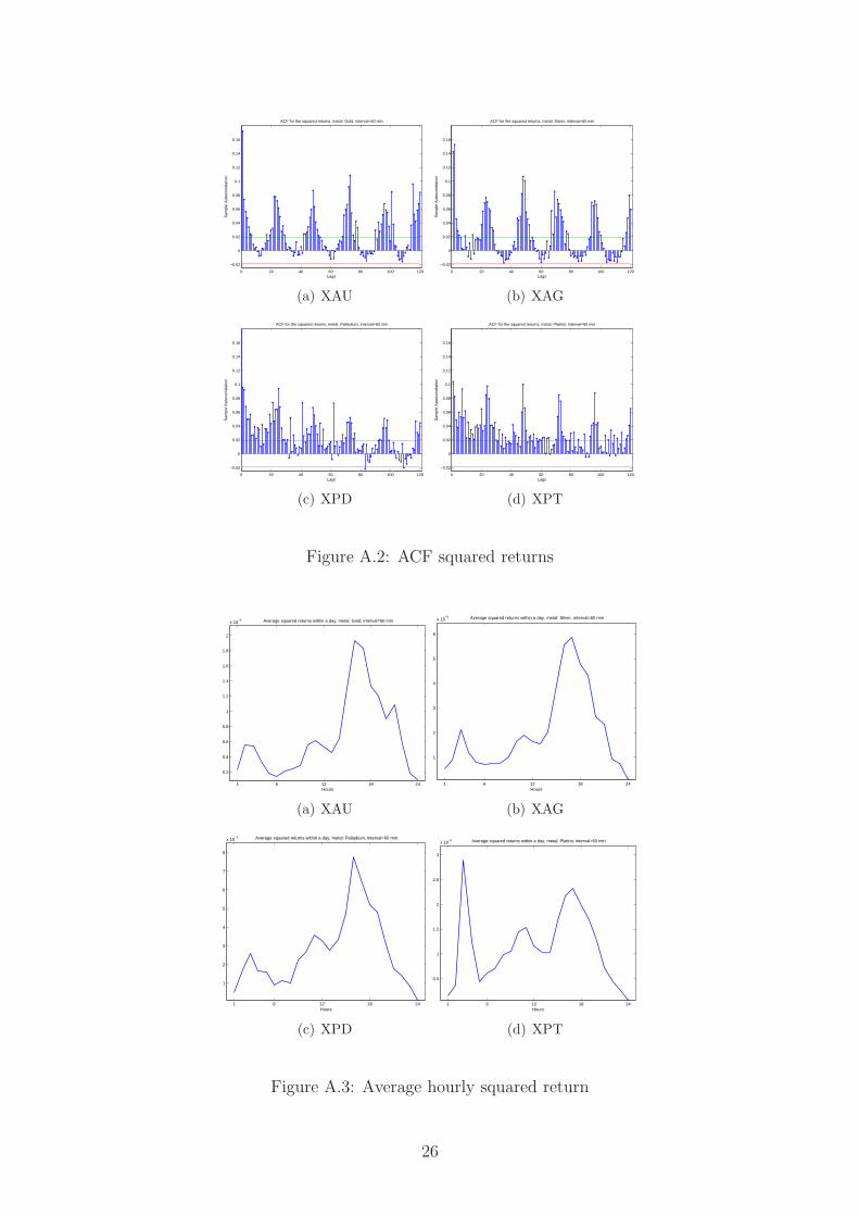
Precious metals returns provide relevant information on the evolution of the condi-tional variances. The analysis of squared returns shows evidence of heteroskedasticty,with a clear periodic behavior (see the upper panel of Figure (3) for the gold time series).The pattern is more regular in the gold and silver cases compared to palladium and plat-inum. This is, however, an expected result and is due to the large number of zeros presentin the last two time series. Similar patterns can be identified at the 5-minute frequencyfor gold and silver. Notably, the oscillations of the ACF have a period of one day (24hours). Confirmation of the periodic evolution of the intradaily variance is given in Figure(4), where we report, for the gold series, the hourly average squared return, computedas r2i =

1T

∑Tt=1 r

2i,t. The graph shows evidence, within the day, of three relevant periods,

which we can associate with the trading activities in different geographical areas. Thefirst increase in volatility corresponds to the Asian markets’ trading activity. The averagesquared returns then decrease until the opening of European markets. The increase peaksaround 10 GMT and then again begins to decrease until 13 GMT. The average returns

8Figure (2) refers to the gold. Similar patterns are present for the other metals, with the largestfrequency of zeros for palladium and platinum. Graphs are available upon request.

9Graphical analyses supporting this claim are available upon request.

8

0

10

20

30

40

50

60

70

80

90

Intervals returns equal to 0 (in percentage) metal: Gold, interval=5 min

Hours

Per

cent

age

(a) 5 min

0

10

20

30

40

50

60

70

80

Intervals returns equal to 0 (in percentage) metal: Gold, interval=60 min

Hours

Per

cent

age

(b) 60 min

Figure 2: Occurrence of zeros during the trading day (5 min and hourly series) - XAU

sharply increase when American markets open and peak when American markets are ac-tive and European markets are closing, around 16 GMT. The same behavior is observedin the other three metals.

The periodic behavior of the intradaily volatility might be estimated and filtered outfrom the returns time series following different approaches.10 Among the possible methods,we mention those of Andersen and Bollerslev (1997a) and Boudt et al. (2011). The firstapproach assumes that returns follow a multiplicative model

ri,t = si,tσi,tηi,t, (1)

where si,t is a periodic deterministic component, σi,t is a GARCH-type variance, andηi,t is a standardized innovation with unit variance. The periodic term si,t is estimatedby means of a parametric regression model. The work of Boudt et al. (2011), despiteusing the same multiplicative model for the return, differs from the parametric approachof Andersen and Bollerslev (1997a) in two elements: First, σi,t is an average volatility fac-tor kept constant in a local window around ri,t, and second, the deterministic componentsi,t is estimated by means of a nonparametric approach. The estimation of the periodiccomponent si,t in Andersen and Bollerlev (1997a) considers a regression on harmonics ofthe log-transformed return series (in deviations from their unconditional mean). However,the large number of zeros present in the precious metal returns makes the method inap-propriate for the analyzes of returns. Nevertheless, we consider a variant of the Andersenand Bollerslev (1997a) approach when dealing with volumes.

Boudt et al. (2011) base the estimation of the periodic component in the intradayvolatility on the standardized high-frequency return (ri,t), where the standardization fac-tor is given by the square root of the normalized realized bipower variation of Barndorff-Nielsen and Sheppard (2004). By construction, ri,t is distributed with mean zero andvariance equal to the squared periodicity factor. Boudt et al. (2011) propose to estimatethe periodic component using a nonparametric estimator of the scale of the standardizedreturns ri,t. They suggest three possible estimators: (1) the nonparametric periodicity

10The same procedures to estimate periodic deterministic components have been implemented indifferent areas. For example, Caporin and Pres (2012) model and forecast wind speed intensity andCaporin and Pres (2011) forecast temperature indices density.

9

24 48 72 96 120−0.1

00.10.2

ACF sq ret

24 48 72 96 120−0.1

00.10.2

ACF st sq ret by RBV

24 48 72 96 120−0.1

00.10.2

ACF st sq ret by RBV and f SD

24 48 72 96 120−0.1

00.10.2

ACF st sq ret by RBV and f ShortH

24 48 72 96 120−0.1

00.10.2

ACF st sq ret by RBV and f WSD

Figure 3: ACF of the squared standardized returns - XAU

estimator SD presented by Taylor and Xu (1997), which is based on the standard devia-tion of returns belonging to a local window, (2) the ShortH estimator for the periodicityfactor, based on the Shortest Half scale estimator (see Boudt et al., 2011, for details), and(3) the Weighted Standard Deviation estimator, WSD, of Boudt et al. (2011). Note thatthe second and third estimators are also robust to the presence of price jumps. Giventhe nonparametric estimators of the periodic component, and similar to the approach ofAndersen and Bollerslev (1997a), it is possible to recover the standardized return series.

Figure (4) displays the estimated periodic component for the hourly return seriesof gold with the three nonparametric methods presented by Boudt et al. (2011). Theplot presents a behavior similar to the average squared returns. However, the ACF ofthe squared returns standardized series (ri,t/si,t) (see Figure (3)), show evidence of someresidual periodic behavior. This finding is not influenced by the estimator adopted tocapture the periodic behavior of squared returns. As a consequence, the nonparametricmethods of Boudt et al. (2011) are not able to completely capture the periodic evolutioncharacterizing the volatility of precious metals returns. This result suggests the possiblepresence of a stochastic behavior in the periodic component, which might be capturedwithin an appropriate time-series framework. In the following section, we propose aparametric model that captures both the periodic evolution and the serial correlation ofsquared returns.

3.2 Volume

The volume time series are characterized by a percentage of zeros comparable to thereturns time series. Note that volume and returns do not necessarily have the same oc-

10

0 5 10 15 20 250

0.02

0.04

0.06

0.08

0.1Non parametric periodic component

0 5 10 15 20 250

1

2

x 10−5

f SDf ShortHf WSDmean

Figure 4: Estimated periodic component, parametric and non parametric approaches -XAU

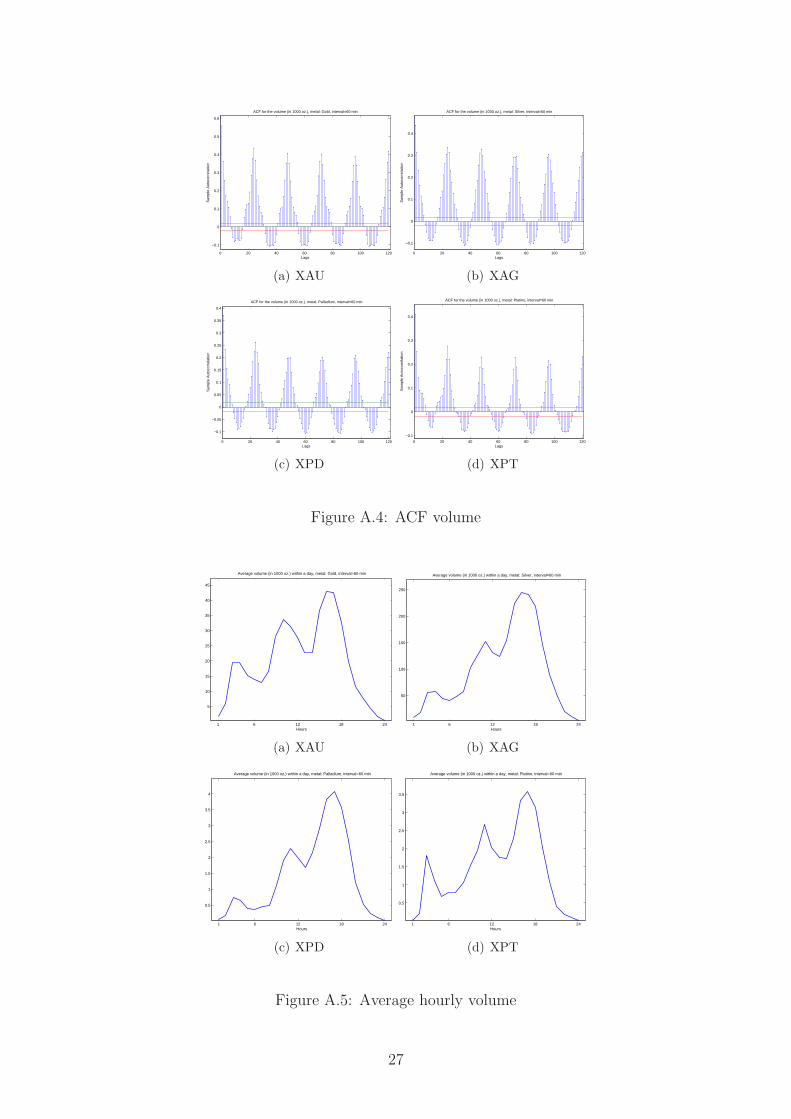
currence of zeros as trades could be executed at the same price over consecutive intradailyperiods. Table (2) presents descriptive analysis of the volume data, measured in numbersof MTA. We observe that the average volume is the highest for silver, at both the 5-and 60-minute frequencies. Moreover, when we recast the MTAs in ounces, we highlightthat gold has the lowest average volume at the 60-minute frequency. This is further con-firmed by the volume quantiles (see Table (2)). The volume time series show evidence ofa strong periodic pattern: The correlograms are characterized by a cyclical behavior, andthe intradaily volume averages, vi =

1T

∑Tt=1 vi,t, are higher during the opening hours of

the most active precious metals markets. The increases in the volume level has a timingcomparable to the increase in squared returns observed in Figure (4).

Similarly to the volatility, the periodic behavior of volume time series might be deter-ministic, stochastic, or a mixture of both deterministic and stochastic elements. Amongthe different approaches that are available to filter the periodic component from volumetime series, we mention the use of seasonal adjustment methods, which can be based onmoving averages or regression approaches and might be either multiplicative or additive.Multiplicative approaches are inappropriate given the large number of zeros, but additivemethods might be more suitable. As a first analysis of volume, we propose the use ofregression methods based on harmonics. We assume that the volume mean is given asfollows (the time index evolves at an intradaily frequency):

vt = α +

p∑

i=1

δiti +

q∑

j=1

(

γjcos

(

2πjt

24

)

+ φjsin

(

2πjt

24

))

+ ζt. (2)

The periodic mean component is composed by a constant, a polynomial trend, and a

11

Order Flow Quoted Spread

XAU XAU XAG XAG XPD XPT XAU XAU XAG XAG XPD XPTFrequency 15 60 15 60 60 60 15 60 15 60 60 60

Mean −0.174 −0.699 0.0007 0.0030 0.1084 0.1733 0.0013 0.0012 0.0035 0.0034 0.0098 0.0052Median 0.0000 0.0000 0.0000 0.0000 0.0000 0.0000 0.0005 0.0006 0.0024 0.0025 0.0073 0.0038Std 3.7337 9.0484 1.0721 2.3514 2.2681 2.5741 0.0049 0.0042 0.0045 0.0039 0.0080 0.0055

Kurtosis 22.350 15.720 57.206 18.481 20.964 21.106 1084.5 1553.0 245.13 85.934 29.615 115.47Skewness −0.342 −0.547 −1.048 −0.093 −0.369 0.7425 26.257 30.551 10.422 7.0002 3.8557 7.755% quant. −6 −14 −1 −4 −3 −3 0.0003 0.0003 0.0010 0.0010 0.0036 0.001650% quant. 0 0 0 0 0 0 0.0005 0.0006 0.0024 0.0025 0.0073 0.003895% quant. 5 12 1 4 3 4 0.0040 0.0035 0.0089 0.0083 0.0242 0.0126n. of 0 18424 2305 35787 5937 6852 5737 0.0000 0.0000 0.0000 0.0000 0.0000 0.0000

Table 3: Descriptive analysis: OF and QS across metals

combination of harmonics that capture the intradaily periodic behavior. The use of har-monics makes the estimation of periodic components similar to that adopted by Andersenand Bollerslev (1997a) for the volatility. We estimate the parameters with ordinary leastsquares (OLS) using robust standard errors due to the possible presence of serial corre-lation and heteroskedasticity in the innovations. We note that the regression providesan expected hourly volume replicating the periodic behavior, but residuals are still char-acterized by a strong periodic evolution. Moreover, the slow decay of both the volumeACF and the volume residuals ACF might suggest the presence of long memory.11 Inthe next section, we consider time-series models that capture both the periodic intradailydynamics and the behavior of the volume.

3.3 Liquidity: Order flow and percentage quoted spread

Moving to the liquidity measures, we first point out a relevant difference between orderflow (OF) and percentage quoted spread (PQS): OF has a number of zeros comparableto those observed for returns and volume (see Table (3)), while the PQS time series doesnot have zeros. This is a consequence of the different NF data used to evaluate the twotime series. In fact, OF comes from trade data, whereas PQS depends on book-level data.OF time series of gold shows evidence of much larger variability, compared with the otherprecious metals. This is a consequence of gold attracting the largest number of trades.Notably, the OF is, on average, negative for gold and positive for silver, platinum, andpalladium.

The OF time series are negatively skewed (with the exception of platinum) and highlyleptokurtic (due to the overconcentration around the mean; see the quantiles reportedin Table (3). The PQS time series have similar unconditional behavior at the 15- and60-minute frequencies (see Table (3)). This result is a by-product of the methodologyadopted to compute these quantities, which are determined as intradaily periods aver-ages. As expected, the spreads are on average smaller for gold and higher for platinumand palladium. The dispersion is minimum for silver and maximum for palladium. The

11The ACF of the residuals and the estimated periodic component for the gold series are available inthe appendix.

12

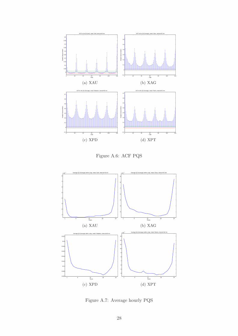
PQS series show evidence of positive asymmetry and of extremely long upper tails (seethe quantiles reported in Table (3)): For Gold at the 15-minute frequency, the averagespread between best bid and ask quotes is around 13 basis points, whereas the upper 99%quantile of PQS reaches the 150 basis points; large values are observed for palladium,where the average spread is close to 100 basis points but peaks at more than 425 basispoints at the 99% quantile. Such large values of the PQS depend on the activity in theEBS platform, which further depends on the timing of the day. In fact, PQS time serieshave a clear intradaily pattern, with the largest values observed between the closing ofAmerican markets and the opening of Asian markets. This pattern is observed in theaverage hourly PQS of gold, QSi =

1T

∑Tt=1 QSi,t, and the ACF of the PQS time series.12

The OF time series do not show peculiar periodic behaviors in their mean, even ifthere is a clear evidence of serial correlation. As a further descriptive analysis, we alsoevaluate the serial correlation and periodic behavior of the squared order flow, which canbe considered a proxy of volatility. In fact, an increase in the order flow, regardless ofthe sign, shows evidence of an increase in trading activity in the market in one specificdirection (either an increase in seller- or buyer-initiated trades). The squared OF has in-tradaily patterns similar to the squared returns, with a clear increase during the openinghours of the most active precious metals markets.

The estimation of the periodic behavior of OF and PQS might follow the same ap-proaches outlined for the returns volatility and the volume. When those approaches areapplied to liquidity measures, the outcome suggests a presence of a periodic behaviorlargely, but not completely, captured by a deterministic approach. We thus apply in thefollowing models whose aim is to estimate both the deterministic and the stochastic be-havior of the series.

4 Dynamic modeling of precious metals time series

The previous section shows that precious metals time series are characterized by peri-odic behaviors. Those patterns are generally captured a priori, before the implementa-tion of dynamic models of the ARMA and GARCH families, which are used to describethe dynamic evolution of high-frequency time series.13 However, the use of alternativemethodologies for filtering periodic patterns leads to standardized series still demonstrat-ing periodic components. Therefore, the use of two-stage estimation methods might notbe appropriate for precious metals time series and calls for time-series models capturingboth the nonperiodic dynamic and the periodic behavior. The literature has proposedseveral models starting with the use of Seasonal ARMA models, with an appropriate se-lection of the period, up to the models with periodic long memory in the mean (Grayet al., 1988, and Woodward et al., 1998). Moreover, Bollerslev and Ghysels (1996),Guegan (2000), and Bordignon et al. (2007, 2009) propose GARCH-type models withperiodic coefficients and periodic long memory. Nevertheless, the periodic behavior andthe nonperiodic dynamic can be captured resorting to models in which the ARMA- and

12Similar patterns are present for silver, palladium, and platinum. Figures are included in the ap-pendix.

13Two-step approaches are computationally simple but imply a loss of efficiency compared with modelswhere periodic patterns are estimated together with the parameters driving the series dynamic.

13

µ φ1 ω θ1 θ2 θ3 θ6 θ12 θ24 β1 β2 β3

−1.4e− 09 −0.038b −0.241 0.123a 0.138b 0.078 −0.009 −0.016c 0.154a 0.007 −0.012c 0.233a

(2.2e− 05) (0.019) (0.383) (0.025) (0.055) (0.053) (0.022) (0.008) (0.042) (0.034) (0.007) (0.058)

β6 β12 β24 γ1 φ1 γ2 φ2 γ3 φ3 γ4 φ4 γ50.190 0.166a 0.390a −0.516a −0.372a −0.123 0.253a −0.177b 0.350a −0.199a −0.014 −0.251a

(0.126) (0.051) (0.091) (0.130) (0.087) (0.105) (0.049) (0.090) (0.048) (0.054) (0.024) (0.046)

φ5 LLF0.140a 56787.14(0.039)

µ φ1 ω θ1 θ2 θ3 θ6 θ12 θ24 β1 β2 β3

−1.4e− 09 −0.038b −0.107 0.139a - 0.097c −0.107b 0.054 0.051 0.625a - −0.243b

(2.2e− 05) (0.019) (0.067) (0.034) (0.056) (0.045) (0.121) (0.193) (0.061) (0.099)

β6 β12 β24 γ1 φ1 γ2 φ2 γ3 φ3 γ4 φ4 γ50.658a −0.779c 0.728 −0.071b −0.138c −0.048a 0.350a −0.040 0.292a −0.257a 0.150a −0.073(0.232) (0.416) (0.526) (0.034) (0.079) (0.014) (0.049) (0.029) (0.033) (0.051) (0.036) (0.048)

φ5 LLF0.257a 56745.73(0.036)

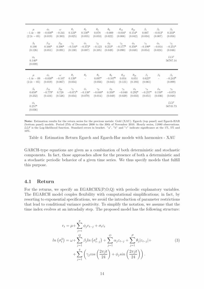
Note: Estimation results for the return series for the precious metals: Gold (XAU). Egarch (top panel) and Egarch-HAR(bottom panel) models. Period 27th of December 2008 to the 30th of November 2010. Hourly series, 11880 observations.LLF is the Log-likelihood function. Standard errors in bracket. ”a”, ”b” and ”c” indicate significance at the 1%, 5% and10%.

Table 4: Estimation Return Egarch and Egarch-Har models with harmonics - XAU

GARCH-type equations are given as a combination of both deterministic and stochasticcomponents. In fact, those approaches allow for the presence of both a deterministic anda stochastic periodic behavior of a given time series. We thus specify models that fulfillthis purpose.

4.1 Return

For the returns, we specify an EGARCHX(P,O,Q) with periodic explanatory variables.The EGARCH model couples flexibility with computational simplifications; in fact, byresorting to exponential specifications, we avoid the introduction of parameter restrictionsthat lead to conditional variance positivity. To simplify the notation, we assume that thetime index evolves at an intradaily step. The proposed model has the following structure:

rt = µ+

p∑

j=i

φjrt−j + σtεt

ln(

σ2t

)

= ω+

Q∑

j=1

βjln(

σ2t−j

)

+

O∑

j=1

αjεt−j +

P∑

j=1

θj|εt−j |+

+

q∑

j=1

(

γjcos

(

2πjt

24

)

+ φjsin

(

2πjt

24

))

.

(3)

14

24 48 72 96 120−0.1

−0.05

0

0.05

0.1

0.15ACF std. residuals EGARCH(1 2 3 6 12 24,1 2 3 6 12 24) AR(1) 5 harm, metal:Gold

24 48 72 96 120−0.1

−0.05

0

0.05

0.1

0.15ACF std. residuals EGARCH HAR (1 3 6 12 24,1 3 6 12 24) AR(1) 5 harm, metal:Gold

(a) XAU

0 5 10 15 20 250

2

4x 10

−5 Mean Estimated series EGARCH and EGARCH HAR, metal:Gold

0 5 10 15 20 250

1

2x 10

−5

EGARCH(1 2 3 6 12 24,1 2 3 6 12 24) AR(1) 5 harmEGARCH HAR(1 3 6 12 24,1 3 6 12 24) AR(1) 5 harm

mean rt2

(b) XAU

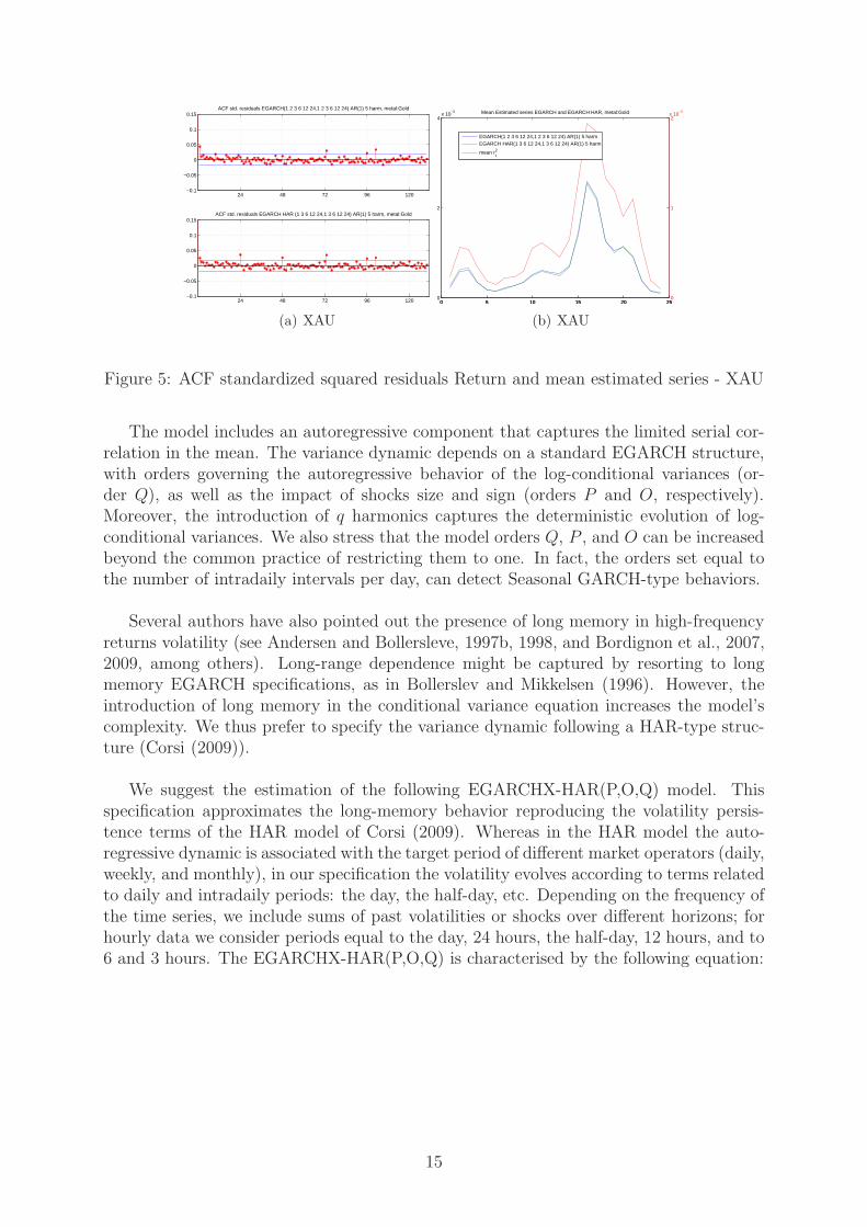
Figure 5: ACF standardized squared residuals Return and mean estimated series - XAU

The model includes an autoregressive component that captures the limited serial cor-relation in the mean. The variance dynamic depends on a standard EGARCH structure,with orders governing the autoregressive behavior of the log-conditional variances (or-der Q), as well as the impact of shocks size and sign (orders P and O, respectively).Moreover, the introduction of q harmonics captures the deterministic evolution of log-conditional variances. We also stress that the model orders Q, P , and O can be increasedbeyond the common practice of restricting them to one. In fact, the orders set equal tothe number of intradaily intervals per day, can detect Seasonal GARCH-type behaviors.

Several authors have also pointed out the presence of long memory in high-frequencyreturns volatility (see Andersen and Bollersleve, 1997b, 1998, and Bordignon et al., 2007,2009, among others). Long-range dependence might be captured by resorting to longmemory EGARCH specifications, as in Bollerslev and Mikkelsen (1996). However, theintroduction of long memory in the conditional variance equation increases the model’scomplexity. We thus prefer to specify the variance dynamic following a HAR-type struc-ture (Corsi (2009)).

We suggest the estimation of the following EGARCHX-HAR(P,O,Q) model. Thisspecification approximates the long-memory behavior reproducing the volatility persis-tence terms of the HAR model of Corsi (2009). Whereas in the HAR model the auto-regressive dynamic is associated with the target period of different market operators (daily,weekly, and monthly), in our specification the volatility evolves according to terms relatedto daily and intradaily periods: the day, the half-day, etc. Depending on the frequency ofthe time series, we include sums of past volatilities or shocks over different horizons; forhourly data we consider periods equal to the day, 24 hours, the half-day, 12 hours, and to6 and 3 hours. The EGARCHX-HAR(P,O,Q) is characterised by the following equation:

15

ln(

σ2t

)

= ω+∑

j=1,3,6,12,24

βj

j

(

ln(

σ2t−j

)

+ ...+ ln(

σ2t−1

))

+

+∑

j=1,3,6,12,24

αj

j(εt−1 + ...+ εt−j) +

∑

j=1,3,6,12,24

θjj(|εt−1|+ ... + |εt−j|)+

+

q∑

j=1

(

γjcos

(

2πjt

24

)

+ φjsin

(

2πjt

24

))

.

(4)

In the analysis of the precious metals returns, we consider different combinations ofthe EGARCHX and EGARCHX-HAR model orders, as well as different number of har-monics. We augment the model by the introduction of an AR(1) term, which is needed tocapture the limited serial correlation observed on mean returns. Table (4) reports the bestspecifications for the gold series. They include five harmonics and lags up to order 24 (theday when focusing on hourly time series). Notably, the shock’s sign was irrelevant (theEGARCHX order O was then set to zero). In both the EGARCHX and EGARCHX-HARspecifications, the lag 24 and the five harmonics parameters are statistically significant.

The left panel of Figure (5) presents ACF of the standardized squared returns ((rt/σt)2)

for the EGARCHX(P,O,Q) and for the EGARCHX HAR(P,O,Q) models. The seasonallyadjusted residual series show evidence of serial correlation for both specifications. Inparticular, the first lag in the EGARCHX specification is significant, and a daily periodicresidual remains in the correlation in the EGARCHX-HAR case. The serial correlationin the ACF of the EGARCHX standardized residuals might signal the existence of mildlong-memory behavior which is not appropriately taken into account by the model. TheEGARCHX-HAR model captures the potential long-range dependence of the volatility,but it is not able to completely remove the periodic component. Similar results areobtained for the other precious metals.

4.2 Volume

As pointed out in the previous section, the volume time series shows evidence supportingthe presence of a stochastic periodic behavior, coupled with the possible presence of long-range dependence.14 To capture such a feature, we consider a multifactor GARMA modelthat allows for long-memory behavior which might be associated with specific periodicfrequencies.

Following Woodward et. al (1998), the multifactor GARMA model is defined by

Φ(L)

h∏

j=0

(1− 2cos(wj)L+ L2)dj (yt − µ) = Θ(L)ǫt, (5)

where h is an integer, ǫt is a white noise with variance σ2ǫ , µ is the mean of the process,

ωj (with j = 0, ..., h) are the frequencies at which the long-memory behavior occurs, dj(with j = 0, ..., h) are the long-memory parameters associated to each frequency, and Φ(L)

14Bollerlsev and Jubinski (1999) and Lobato and Velasco (2000), among others, document long memoryin stock-market trading volume.

16

d1 d2 d3 d4 d5 d6 d7 d8 d9 d10 d11 d120.292a 0.468a 0.382a 0.362a 0.368a 0.317a 0.323a 0.320a 0.314a 0.316a 0.313a 0.293a

(0.008) (0.031) (0.035) (0.081) (0.053) (0.046) (0.055) (0.059) (0.061) (0.108) (0.057) (0.107)

d13 φ1 φ24 φ48 φ72 φ96 φ120 θ1 µ σ2ǫ LLF

0.143a −0.018 −0.257a −0.150a −0.097c −0.070a −0.002 −0.517a −26.62a 356.8a -51768.53(0.010) (0.159) (0.069) (0.025) (0.055) (0.013) (0.061) (0.104) (6.688) (35.77)

Note: Estimation results for the volume series for the precious metals: Gold (XAU). GARMA models. Period 27th ofDecember 2008 to the 30th of November 2010. Hourly series, 11880 observations. LLF is the Log-likelihood function.Standard errors in bracket. ”a”, ”b” and ”c” indicate significance at the 1%, 5% and 10%.

Table 5: Estimation Volume GARMA model - XAU

24 48 72 96 120

−0.1

−0.05

0

0.05

0.1

0.15

Lag

ACF std. residuals GARMA 24 ARMA(0,0), metal:Gold

24 48 72 96 120

−0.1

−0.05

0

0.05

0.1

0.15

Lag

ACF std. residuals GARMA 24 ARMA(1 24 48 72 96 120,1), metal:Gold

(a) XAU

0 5 10 15 20 250

10

20

30

40

50

Hours

Mean Estimated series, metal:Gold

0 5 10 15 20 250

10

20

30

40

50

GARMA 24 ARMA(0,0)GARMA 24 ARMA(1 24 48 72 96 120,1)mean Vol

(b) XAU

Figure 6: ACF standardized squared residuals Volume and mean estimated series - XAU

and Θ(L) are the short-memory autoregressive and moving average polynomials with rootssatisfying the usual stationarity and invertibility conditions. Stationarity of the GARMAmodel is achieved if the memory coefficients assume values below 0.5 for 1 ≤ j ≤ h − 1and below 0.25 for j = 0 and j = h (see Woodward et al., 1998). The most relevantelement of the multifactor GARMA model is the so-called Gegenbauer polynomial, givenby

P (L) =

h∏

j=0

(1− 2cos(wj)L+ L2)dj , (6)

which may be considered as a generalized long-memory filter for the long-memoryperiodic behavior at h + 1 frequencies. The ωj’s are the driving frequencies of a cyclicalpattern of length S, where ωj = (2πj/S), h + 1 = [S/2] + 1, and [·] refers to the integerpart. Previous studies have shown that the GARMA model is able to replicate the peri-odic patterns similar to those observed in the volume time series (see Bordignon et al.,2007 and 2009). To estimate the (h + 1)-factor GARMA model in (5), we implement anautoregressive approximation technique. Following Chung (1996), it is in fact possible torecover an MA(∞) or AR(∞) expansion of the model, and thus to estimate the modelparameters through a quasi-maximum likelihood (QML) approach.

As previously observed, the autocorrelation function oscillates and decays slowly to-

17

d φ1 φ24 φ48 φ72 φ96 φ120 θ1 µ γ1 φ1 γ20.076a −0.072a 0.090a 0.036a 0.049a 0.070a 0.292a 0.227a −0.134a −0.120a 0.014 −0.101a

(0.010) (0.022) (0.008) (0.008) (0.008) (0.008) (0.008) (0.022) (0.014) (0.011) (0.011) (0.011)

φ2 γ3 φ3 γ4 φ4 γ5 φ5 σ2ǫ LLF

−0.002 −0.085a −0.005 −0.071a −0.009 −0.057a −0.011 0.128a -4674.295(0.011) (0.010) (0.010) (0.010) (0.010) (0.010) (0.010) (0.001)

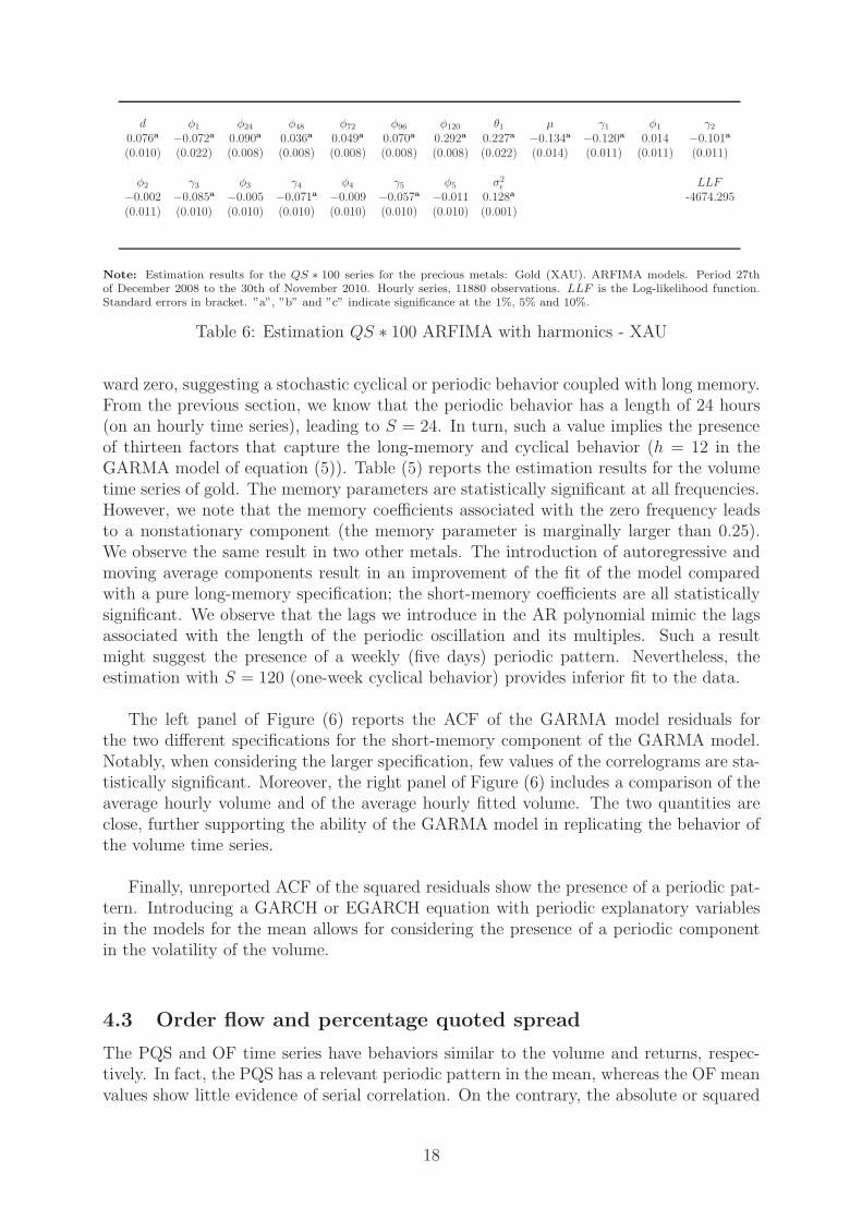
Note: Estimation results for the QS ∗ 100 series for the precious metals: Gold (XAU). ARFIMA models. Period 27thof December 2008 to the 30th of November 2010. Hourly series, 11880 observations. LLF is the Log-likelihood function.Standard errors in bracket. ”a”, ”b” and ”c” indicate significance at the 1%, 5% and 10%.

Table 6: Estimation QS ∗ 100 ARFIMA with harmonics - XAU

ward zero, suggesting a stochastic cyclical or periodic behavior coupled with long memory.From the previous section, we know that the periodic behavior has a length of 24 hours(on an hourly time series), leading to S = 24. In turn, such a value implies the presenceof thirteen factors that capture the long-memory and cyclical behavior (h = 12 in theGARMA model of equation (5)). Table (5) reports the estimation results for the volumetime series of gold. The memory parameters are statistically significant at all frequencies.However, we note that the memory coefficients associated with the zero frequency leadsto a nonstationary component (the memory parameter is marginally larger than 0.25).We observe the same result in two other metals. The introduction of autoregressive andmoving average components result in an improvement of the fit of the model comparedwith a pure long-memory specification; the short-memory coefficients are all statisticallysignificant. We observe that the lags we introduce in the AR polynomial mimic the lagsassociated with the length of the periodic oscillation and its multiples. Such a resultmight suggest the presence of a weekly (five days) periodic pattern. Nevertheless, theestimation with S = 120 (one-week cyclical behavior) provides inferior fit to the data.

The left panel of Figure (6) reports the ACF of the GARMA model residuals forthe two different specifications for the short-memory component of the GARMA model.Notably, when considering the larger specification, few values of the correlograms are sta-tistically significant. Moreover, the right panel of Figure (6) includes a comparison of theaverage hourly volume and of the average hourly fitted volume. The two quantities areclose, further supporting the ability of the GARMA model in replicating the behavior ofthe volume time series.

Finally, unreported ACF of the squared residuals show the presence of a periodic pat-tern. Introducing a GARCH or EGARCH equation with periodic explanatory variablesin the models for the mean allows for considering the presence of a periodic componentin the volatility of the volume.

4.3 Order flow and percentage quoted spread

The PQS and OF time series have behaviors similar to the volume and returns, respec-tively. In fact, the PQS has a relevant periodic pattern in the mean, whereas the OF meanvalues show little evidence of serial correlation. On the contrary, the absolute or squared

18

values of OF are characterized by a strong periodic behavior. Moreover, deterministic pe-riodic filters are not effective in removing the periodic behavior of the liquidity time series.Given these findings, the liquidity measures’ dynamic features might be captured usingthe approaches we consider for the volume and returns cases, that is the GARMA andEGARCH specifications. As an alternative methodology, we consider the ARFIMA andSeasonal ARFIMA (SARFIMA) models extended with the inclusion of periodic explana-tory mean variables. We estimate these two models on the PQS mean and on the squaredOF values. The SARFIMA is a special case of the multifactor GARMA model. Similarto the most general model, it provides periodic behavior coupled with long memory. TheSARFIMA model is given as follows:

Φ(L)(1 − LS)d(yt − µ−

q∑

j=1

(

γjcos

(

2πjt

24

)

+ φjsin

(

2πjt

24

))

) = Θ(L)ǫt, (7)

where ǫt is a white noise with variance σ2ǫ . The autoregressive and moving average

polynomials Φ(L) and Θ(L) satisfy the usual restrictions for stationarity and invertibil-ity, whereas the memory parameter d gives a stationary model if its value is below 0.5.The seasonal long-memory behavior influences the observed variable yt in deviation fromits unconditional mean µ and from a deterministic periodic behavior captured by theq harmonics. The relation between SARFIMA and GARMA is given by the followingdecomposition of the seasonal long-memory filter

(1−LS) =(

1− 2cos (ω0)L+ L2)

1

2

[

S−1∏

j=1

(

1− 2cos (ωj)L+ L2)

]

(

1− 2cos (ωs)L+ L2)

1

2 ,

(8)where ω0 = 1 and ωs = −1 . The previous decomposition takes into account the roots

of the polynomial(

1− LS)

, which are associated with frequencies in 0−π. In particular,the frequencies are 0, π (if S is even), and a set of frequencies depending on the value ofS, each associated with a pair of roots of the polynomial. Notably, such a decompositioncorresponds to a product of Gegenbauer polynomials. If we introduce long memory and

consider(

1− LS)d, the exponent of each Gegenbauer polynomial in (8) is either equal to

d or to d/2 (this happen for frequencies ω0 and ω1). As a consequence, the SARFIMAmodel is a special case of the multifactor GARMA under a restriction on the memory co-efficient, and if the frequencies over which the GARMA model is specified are exactly thesame set of frequencies associated with the decomposition of the seasonal filter

(

1− LS)

.

In the analysis of the liquidity series,15 we consider different specifications for themodels. We set three different values for the seasonal length (S) 1, 24, and 120. WithS = 1, we specify a pure long-memory model for the hourly series, whereas in the caseof S = 24 or 120, we specify a daily and weekly seasonal integration pattern. To cap-ture the periodic behavior of the series, we consider up to six daily harmonics, and weinclude a weekly harmonic. Finally, to model the short-memory component, we introducedifferent autoregressive and moving average specifications, considering lags up to the week.

15The estimated series are equal to QS × 100 and OF 2/100, respectively.

19

24 48 72 96 120−0.1

−0.05

0

0.05

0.1

0.15

Hours

ACF std. residuals ARFIMA(1 24 120,1,1) 5 harm, metal:Gold

24 48 72 96 120−0.1

−0.05

0

0.05

0.1

0.15

Hours

ACF std. residuals ARFIMA(1 24 48 72 96 120,1,1) 5 harm, metal:Gold

(a) XAU

0 5 10 15 20 250

0.1

0.2

0.3

0.4

0.5

0.6

0.7

0.8

0.9

Hours

Mean Estimated series, metal:Gold

ARFIMA(1 24 120,1,1) 5 harmARFIMA(1 24 48 72 96 120,1,1) 5 harmmean QS

(b) XAU

Figure 7: ACF standardized squared residuals QS and mean estimated series - XAU

d φ1 φ24 φ48 φ72 φ96 φ120 θ1 µ γ1 φ1 γ20.046a 0.294a 0.029a 0.027a 0.021b 0.020b 0.048a −0.191a −0.826a 0.587a 0.452a 0.309a

(0.014) (0.062) (0.008) (0.008) (0.008) (0.008) (0.008) (0.058) (0.061) (0.059) (0.059) (0.055)

φ2 γ3 φ3 γ4 φ4 γ5 φ5 σ2ǫ LLF

−0.268a −0.150a −0.245a 0.093c 0.237a 0.017 −0.013 9.220a -30052.31(0.055) (0.051) (0.051) (0.048) (0.048) (0.045) (0.045) (0.119)

Note: Estimation results for the OF 2/100 series for the precious metals: Gold (XAU).ARFIMA models. Period 27thof December 2008 to the 30th of November 2010. Hourly series, 11880 observations. LLF is the Log-likelihood function.Standard errors in bracket. ”a”, ”b” and ”c” indicate significance at the 1%, 5% and 10%.

Table 7: Estimation OF 2/100 ARFIMA with harmonics - XAU

For the QS, Table (6) presents the results of the model that best fits the gold series.Although we try with the ARFIMA and SARFIMA models, we concentrate on the firstkind of models (S = 1). Estimation results and the ACF of the residuals of SARFIMAmodels are similar. The long-memory parameter is significant for all the metals, but it islower for gold than the other three metals. In the first case, it is equal to 0.076 whereasit is near 0.28 for silver and palladium and 0.493 for platinum. The introduction of theautoregressive lags improves the fitting of the model. Note that the lags are all statisti-cally significant.16 The analysis of the ACF of the residuals, in the left panel of Figure(7), favors the introduction of short-memory component at the daily and its multiplelags. Moreover, it displays significant correlations associated with particular lags. Thisfact is more evident in the gold series. We believe they are neither associated with thelong-memory component nor with the periodic pattern, which have both been correctlyremoved. The right panel of Figure (7) presents the mean fitted series, which replicatesthe periodic component observed in the QS time series.

For the OF 2, Table (7) displays the estimation result for the gold series. As in theprevious case, we consider ARFIMA and Seasonal ARFIMA specifications and we findvery similar outcomes. Then we focus on the pure long-memory model (S = 1). Esti-

16A likelihood ratio test between an ARFIMA(1 24 48 72 96 120,d,1) and ARFIMA(1 24 120,d,1)specification rejects the restricted model in the four metals at 5% level.

20

24 48 72 96 120−0.1

−0.05

0

0.05

0.1

0.15

Hours

ACF std. residuals ARFIMA(1 24 120,1,1) 5 harm, metal:Gold

24 48 72 96 120−0.1

−0.05

0

0.05

0.1

0.15

Hours

ACF std. residuals ARFIMA(1 24 48 72 96 120,1,1) 5 harm, metal:Gold

(a) XAU

0 5 10 15 20 25−0.5

0

0.5

1

1.5

2

2.5

Hours

Mean Estimated series, metal:Gold

ARFIMA(1 24 120,1,1) 5 harmARFIMA(1 24 48 72 96 120,1,1) 5 harm

mean OF2

(b) XAU

Figure 8: ACF standardized squared residuals OF 2 and mean estimated series - XAU

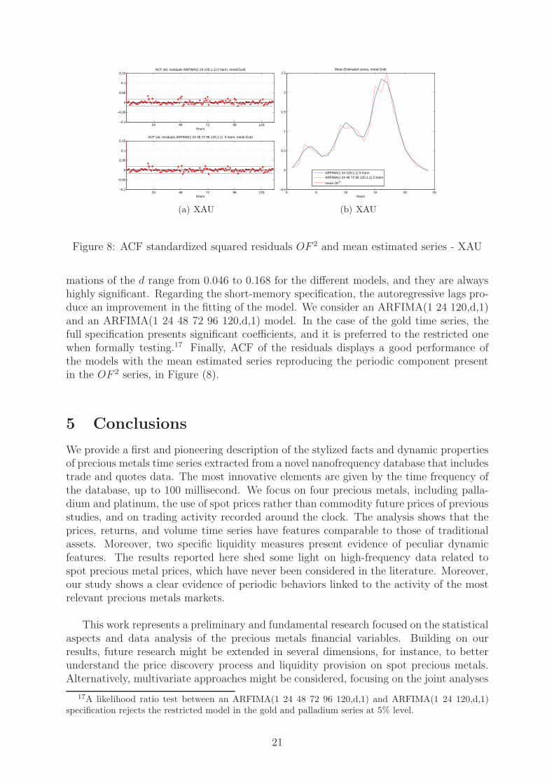
mations of the d range from 0.046 to 0.168 for the different models, and they are alwayshighly significant. Regarding the short-memory specification, the autoregressive lags pro-duce an improvement in the fitting of the model. We consider an ARFIMA(1 24 120,d,1)and an ARFIMA(1 24 48 72 96 120,d,1) model. In the case of the gold time series, thefull specification presents significant coefficients, and it is preferred to the restricted onewhen formally testing.17 Finally, ACF of the residuals displays a good performance ofthe models with the mean estimated series reproducing the periodic component presentin the OF 2 series, in Figure (8).

5 Conclusions

We provide a first and pioneering description of the stylized facts and dynamic propertiesof precious metals time series extracted from a novel nanofrequency database that includestrade and quotes data. The most innovative elements are given by the time frequency ofthe database, up to 100 millisecond. We focus on four precious metals, including palla-dium and platinum, the use of spot prices rather than commodity future prices of previousstudies, and on trading activity recorded around the clock. The analysis shows that theprices, returns, and volume time series have features comparable to those of traditionalassets. Moreover, two specific liquidity measures present evidence of peculiar dynamicfeatures. The results reported here shed some light on high-frequency data related tospot precious metal prices, which have never been considered in the literature. Moreover,our study shows a clear evidence of periodic behaviors linked to the activity of the mostrelevant precious metals markets.

This work represents a preliminary and fundamental research focused on the statisticalaspects and data analysis of the precious metals financial variables. Building on ourresults, future research might be extended in several dimensions, for instance, to betterunderstand the price discovery process and liquidity provision on spot precious metals.Alternatively, multivariate approaches might be considered, focusing on the joint analyses

17A likelihood ratio test between an ARFIMA(1 24 48 72 96 120,d,1) and ARFIMA(1 24 120,d,1)specification rejects the restricted model in the gold and palladium series at 5% level.

21

on different precious metals or on models capturing the interdependence between returns,volume, volatility, and liquidity.

References

[1] Abergel, F., Bouchaud, J., Foucault, T., Lehalle, C., and Rosenbaum, M., 2012,Market Microstructure: Confronting Many Viewpoints, Wiley.

[2] Andersen, T.G., and Bollerslev, T., 1997a, Intraday periodicity and volatility per-sistence in financial markets, Journal of Empirical Finance 4, 115-158.

[3] Andersen, T.G., and Bollerslev, T., 1997b, Heterogeneous information arrivals andreturn volatility dynamics: uncovering the long run in high volatility returns. Jour-nal of Finance, 52, 975-1005.

[4] Andersen, T.G., and Bollerslev, T., 1998, Answering the skeptics: Yes, standardvolatility models do provide accurate forecasts, International Economic Review, 39,885-905.

[5] Andersen, T.G., Bollerslev, T., Diebold, F.X., and Vega, C., 2003, Micro effectsof macro announcements: real-time price discovery in foreign exchange, AmericanEconomic Review, 93, 38-62.

[6] Baillie, R.T., Han, Y., Myers, R.J., and Song, J., 2007, Long-memory models fordaily and high-frequency commodity future returns, Journal of Future Markets,27-7, 643-668.

[7] Bannouh, K., van Dijk, D., and Martens, M., 2009, Range-Based Covariance Esti-mation Using High-Frequency Data: The Realized Co-Range, Journal of FinancialEconometrics, 7-4, 341-372.

[8] Barkoulas, J., Labys, W.C., Onochie, J., 1997, Fractional Dynamics in InternationalCommodity Prices. Journal of Future Markets, 17-2, 161-189.

[9] Barndorff-Nielsen, O.E., and Shephard, N., 2004, Power and bipower variation withstochastic volatility and jumps, Journal of Financial Econometrics, 2, 1-37.

[10] Bauwens, L., and Giot, P., 2001, Econometric modeling of stock market intradayactivity, Kluwer, Dordrecht.

[11] Bekaert, G., Harvey, C., and Lundblad, C., 2007, Liquidity and Expected Returns:Lessons from Emerging Markets, Review of Financial Studies, 20-6, 1783-1831.

[12] Berger, D.W., Chaboud, A.P., Chernenko, S.V., Howorka, E., and Wright,J.H.,2008, Order Flow and Exchange Rate Dynamics in Electronic Brokerage SystemData, Journal of International Economics, 75, 93-109.

[13] Bollerslev, T., and Domowitz, I., 1993, Trading Patterns and Prices in the InterbankForeign Exchange Market, Journal of Finance, 48, 1421-43.

[14] Bollerslev, T., and Ghysel, E., 1996, Periodic Autoregressive Conditional Het-eroscedasticity, Journal of Business and Economic Statistics, 14, 139-151.

22

[15] Bollerlsev, T., and Jubinski, D., 1999, Equity Trading Volume and Volatility: LatentInformation Arrivals and Common Long-Run Dependencies, Journal of Business andEconomic Statistics, 17-1, 9-21.

[16] Bollerslev, T., and Mikkelsen, H.O., 1996, Modeling and pricing long memory instock market volatility. Journal of Econometrics, 73, 151-184.

[17] Bordignon, S., Caporin, M., and Lisi, F., 2007, Generalised Long Memory GARCHmodels for intradaily volatility, Computational Statistics & Data Analysis, 51-12,5900-5912.

[18] Bordignon, S., Caporin, M., and Lisi, F., 2009, Periodic Long Memory GARCHmodels, Econometric Reviews, 28, 60-82.

[19] Boudt, K, Croux, C., and Laurent, S., 2011, Robust estimation of intraweek peri-odicity in volatility and jump detection, Journal of Empirical Finance, 18, 353-367.

[20] Brownlees, C.T., and Gallo, G.M., 2006, Financial econometric analysis at ultra-high-frequency: Data handling concerns, Computational Statistics & Data Analysis,51 - 4, 2232-2245.

[21] Cai, J., Cheung, Y., and Song, M.C.S., 2001, What Moves the Gold Market?,Journal of Future Markets, 21-3, 257-278.

[22] Caporin, M., and Pres, J., 2011, Forecasting Temperature Indices Density withTime-Varying Long-Memory Models, Journal of Forecasting.

[23] Caporin, M., and Pres, J., 2012, modeling and forecasting wind speed intensityfor weather risk management, Computational Statistics & Data Analysis, 56 - 11,3459-3476.

[24] Corsi, F., 2009, A simple approximate long-memory model of realized volatility.Journal of Financial Econometrics, 7, 174-196.

[25] Chung, C., 1996, Estimating a generalized long memory process. Journal of Econo-metrics, 73, 237-259.

[26] Dacorogna, M.M., Muller U.A., Nagler, R.J., Olsen, R.B., Pictet, O.V., 1993, A ge-ographical model for the daily and weekly seasonal volatility in the foreign exchangemarket, Journal of International Money and Finance 12, 413-438.

[27] Dacorogna, M.M., Gencay, R., Muller, U.A., Olsen, R., Pictet, O.V., 2001, Anintroduction to high-frequency finance, Academic Press, London.

[28] Engle, R.F., Russell, J.R., 2009, Analysis of high-frequency Data, Handbook ofFinancial Econometrics, Eds. Y. Ait-Sahalia and L.P. Hansen, Elsevier, North Hol-land.

[29] Fleming, J., Kirby, C., and Ostdiek, B., 2003, The economic value of volatilitytiming using realized volatility, Journal of Financial Economics, 67, 473-509.

[30] Flood, M.D., 1994, Market structure and inefficiency in the foreign exchange market,Journal of International Money and Finance, 13, 131-158.

23

[31] Gabrielsen, A., Marzo, M., and Zagaglia, P., 2011, Measuring market liquid-ity: an introductory survey, MPRA paper 35829, available at http://mpra.ub.uni-muenchen.de/35829/

[32] Gray, H.L., Zhang, N., and Woodward, W., 1988, On generalized fractional pro-cesses, Journal of Time Series Analysis, 10, 233-257.

[33] Guegan, D., 2000, A new model: the k-factor GIGARCH process, Journal of SignalProcessing 4, 265-271.

[34] Hasbrouck, J., 2007, Empirical Market Microstructure: The Institutions, Eco-nomics, and Econometrics of Securities Trading, Oxford University Press, USA.

[35] Hautsch, N., 2011, Econometrics of financial high-frequency data, Springer.

[36] Khalifa, A.A.A., Miao, H., and Ramchander, S., 2011, Return distribution andvolatility forecasting in metal futures markets: evidence from gold, silver and copper,Journal of Future Markets, 31-1, 55-80.

[37] Lee, C., and Ready, M., 1991, Inferring Trade Direction from Intraday Data, Journalof Finance, 46, 733-746.

[38] Lobato, I., and Velasco, C., 2000, Long Memory in Stock-Marcket Trading Volume,Journal of Business and Economic Statistics, 18-4, 410-427.

[39] Mancini, L., Ranaldo, A., and Wrampelmeyer, J., 2012, Liquidity in the ForeignExchange Market: Measurement, Commonality, and Risk Premiums, Journal ofFinance, forthcoming.

[40] O’Hara, M., 1997, Market Microstructure, Blackwell, London.

[41] Parlour, C.A., and Seppi, D.J., Limit order markets: a survey, Handbook of finan-cial intermediation and banking, Thakor, A.V., and Boot A.W.A. (Eds.), North-Holland, Elsevier, Amsterdam.

[42] Schmidt, A., 2011, Financial Markets and Trading: An Introduction to MarketMicrostructure and Trading Strategies, Wiley.

[43] Taylor, S.J., and Xu, X., 1997, The incremental volatility information in one millionforeign exchange quotations, Journal of Empirical Finance 4, 317-340.

[44] Woodward, W.A., Cheng, Q.C., and Gray, H., 1998, A k-factor GARMA long-memory model, Journal of Time Series Analysis 19, 485-504.

[45] Ye, G., 2011, high-frequency trading models, Wiley.

24

A Web Appendix18

0

10

20

30

40

50

60

70

80

Intervals returns equal to 0 (in percentage) metal: Gold, interval=60 min

Hours

Per

cent

age

(a) XAU

0

10

20

30

40

50

60

70

80

90

Intervals returns equal to 0 (in percentage) metal: Silver, interval=60 min

Hours

Per

cent

age

(b) XAG

0

10

20

30

40

50

60

70

80

90

Intervals returns equal to 0 (in percentage) metal: Palladium, interval=60 min

Hours

Per

cent

age

(c) XPD

0

10

20

30

40

50

60

70

80

90

Intervals returns equal to 0 (in percentage) metal: Platino, interval=60 min

Hours

Per

cent

age

(d) XPT

Figure A.1: Occurrence of zeros during the trading day (hourly series)

18Additional tables and figures not included in the paper.

25

0 20 40 60 80 100 120

−0.02

0

0.02

0.04

0.06

0.08

0.1

0.12

0.14

0.16

ACF for the squared returns, metal: Gold, interval=60 min

Lags

Sam

ple

Aut

ocor

rela

tion

(a) XAU

0 20 40 60 80 100 120

−0.02

0

0.02

0.04

0.06

0.08

0.1

0.12

0.14

0.16

ACF for the squared returns, metal: Silver, interval=60 min

Lags

Sam

ple

Aut

ocor

rela

tion

(b) XAG

0 20 40 60 80 100 120

−0.02

0

0.02

0.04

0.06

0.08

0.1

0.12

0.14

0.16

ACF for the squared returns, metal: Palladium, interval=60 min

Lags

Sam

ple

Aut

ocor

rela

tion

(c) XPD

0 20 40 60 80 100 120

−0.02

0

0.02

0.04

0.06

0.08

0.1

0.12

0.14

0.16

ACF for the squared returns, metal: Platino, interval=60 min

Lags

Sam

ple

Aut

ocor

rela

tion

(d) XPT

Figure A.2: ACF squared returns

1 6 12 18 24

0.2

0.4

0.6

0.8

1

1.2

1.4

1.6

1.8

2

x 10−5 Average squared returns within a day, metal: Gold, interval=60 min

Hours

(a) XAU

1 6 12 18 24

1

2

3

4

5

6

x 10−5 Average squared returns within a day, metal: Silver, interval=60 min

Hours

(b) XAG

1 6 12 18 24

1

2

3

4

5

6

7

8

x 10−5 Average squared returns within a day, metal: Palladium, interval=60 min

Hours

(c) XPD

1 6 12 18 24

0.5

1

1.5

2

2.5

3

x 10−5 Average squared returns within a day, metal: Platino, interval=60 min

Hours

(d) XPT

Figure A.3: Average hourly squared return

26

0 20 40 60 80 100 120

−0.1

0

0.1

0.2

0.3

0.4

0.5

0.6

ACF for the volume (in 1000 oz.), metal: Gold, interval=60 min

Lags

Sam

ple

Aut

ocor

rela

tion

(a) XAU

0 20 40 60 80 100 120

−0.1

0

0.1

0.2

0.3

0.4

ACF for the volume (in 1000 oz.), metal: Silver, interval=60 min

Lags

Sam

ple

Aut

ocor

rela

tion

(b) XAG

0 20 40 60 80 100 120

−0.1

−0.05

0

0.05

0.1

0.15

0.2

0.25

0.3

0.35

0.4

ACF for the volume (in 1000 oz.), metal: Palladium, interval=60 min

Lags

Sam

ple

Aut

ocor

rela

tion

(c) XPD

0 20 40 60 80 100 120

−0.1

0

0.1

0.2

0.3

0.4

ACF for the volume (in 1000 oz.), metal: Platino, interval=60 min

Lags

Sam

ple

Aut

ocor

rela

tion

(d) XPT

Figure A.4: ACF volume

1 6 12 18 24

5

10

15

20

25

30

35

40

45

Average volume (in 1000 oz.) within a day, metal: Gold, interval=60 min

Hours

(a) XAU

1 6 12 18 24

50

100

150

200

250

Average volume (in 1000 oz.) within a day, metal: Silver, interval=60 min

Hours

(b) XAG

1 6 12 18 24

0.5

1

1.5

2

2.5

3

3.5

4

Average volume (in 1000 oz.) within a day, metal: Palladium, interval=60 min

Hours

(c) XPD

1 6 12 18 24

0.5

1

1.5

2

2.5

3

3.5

Average volume (in 1000 oz.) within a day, metal: Platino, interval=60 min

Hours

(d) XPT

Figure A.5: Average hourly volume

27

0 20 40 60 80 100 120

0

0.05

0.1

0.15

0.2

0.25

0.3

0.35

0.4

0.45

0.5

ACF for the QS (end), metal: Gold, interval=60 min

Lags

Sam

ple

Aut

ocor

rela

tion

(a) XAU

0 20 40 60 80 100 120−0.1

0

0.1

0.2

0.3

0.4

0.5

0.6

ACF for the QS (Average), metal: Silver, interval=60 min

Lags

Sam

ple

Aut

ocor

rela

tion

(b) XAG

0 20 40 60 80 100 120−0.1

0

0.1

0.2

0.3

0.4

0.5

0.6

0.7

ACF for the QS (Average), metal: Palladium, interval=60 min

Lags

Sam

ple

Aut

ocor

rela

tion

(c) XPD

0 20 40 60 80 100 120−0.1

0

0.1

0.2

0.3

0.4

0.5

0.6

0.7

ACF for the QS (Average), metal: Platino, interval=60 min

Lags

Sam

ple

Aut

ocor

rela

tion

(d) XPT

Figure A.6: ACF PQS

1 6 12 18 24

1

2

3

4

5

6

7

8

x 10−3 Average QS (Average) within a day, metal: Gold, interval=60 min

Hours

(a) XAU

1 6 12 18 24

3

4

5

6

7

8

9

x 10−3 Average QS (Average) within a day, metal: Silver, interval=60 min

Hours

(b) XAG

1 6 12 18 240.006

0.008

0.01

0.012

0.014

0.016

0.018

0.02

0.022

Average QS (Average) within a day, metal: Palladium, interval=60 min

Hours

(c) XPD

1 6 12 18 24

4

5

6

7

8

9

10

11

12

13

x 10−3 Average QS (Average) within a day, metal: Platino, interval=60 min

Hours

(d) XPT

Figure A.7: Average hourly PQS

28

0 20 40 60 80 100 120

0

0.05

0.1

0.15

0.2

ACF for the OF squared, metal: Gold, interval=60 min

Lags

Sam

ple

Aut

ocor

rela

tion

(a) XAU

0 20 40 60 80 100 120

−0.04

−0.02

0

0.02

0.04

0.06

0.08

0.1

0.12

0.14

ACF for the OF squared, metal: Silver, interval=60 min

Lags

Sam

ple

Aut

ocor

rela

tion

(b) XAG

0 20 40 60 80 100 120

−0.04

−0.02

0

0.02

0.04

0.06

0.08

0.1

0.12

0.14

0.16

ACF for the OF squared, metal: Palladium, interval=60 min

Lags

Sam

ple

Aut

ocor

rela

tion

(c) XPD

0 20 40 60 80 100 120

−0.02

0

0.02

0.04

0.06

0.08

0.1

0.12

ACF for the OF squared, metal: Platino, interval=60 min

Lags

Sam

ple

Aut

ocor

rela

tion

(d) XPT

Figure A.8: ACF OF squared

1 6 12 18 24

50

100

150

200

250

Average OF squared within a day, metal: Gold, interval=60 min

Hours

(a) XAU

1 6 12 18 24

2

4

6

8

10

12

14

Average OF squared within a day, metal: Silver, interval=60 min

Hours

(b) XAG

1 6 12 18 24

2

4

6

8

10

12

14

16

Average OF squared within a day, metal: Palladium, interval=60 min

Hours

(c) XPD

1 6 12 18 24

2

4

6

8

10

12

14

16

18

Average OF squared within a day, metal: Platino, interval=60 min

Hours

(d) XPT

Figure A.9: Average hourly OF squared

29

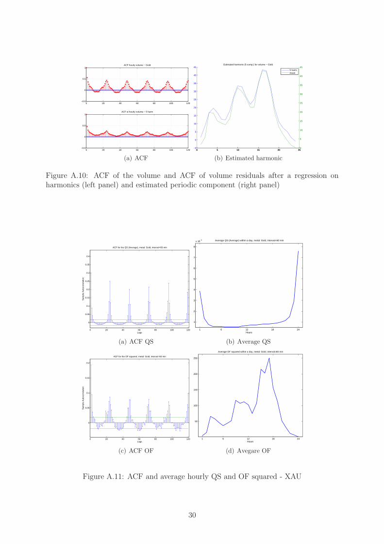
0 20 40 60 80 100 120−0.5

0

0.5

1ACF hourly volume − Gold

0 20 40 60 80 100 120−0.5

0

0.5

1ACF st hourly volume − 5 harm

(a) ACF

0 5 10 15 20 25−5

0

5

10

15

20

25

30

35

40

45Estimated harmonic (5 comp.) for volume − Gold

0 5 10 15 20 250

5

10

15

20

25

30

35

40

455 harm.mean

(b) Estimated harmonic

Figure A.10: ACF of the volume and ACF of volume residuals after a regression onharmonics (left panel) and estimated periodic component (right panel)

0 20 40 60 80 100 120

0

0.05

0.1

0.15

0.2

0.25

0.3

0.35

0.4

ACF for the QS (Average), metal: Gold, interval=60 min

Lags

Sam

ple

Aut

ocor

rela

tion

(a) ACF QS

1 6 12 18 24

1

2

3

4

5

6

7

8

x 10−3 Average QS (Average) within a day, metal: Gold, interval=60 min

Hours

(b) Average QS

0 20 40 60 80 100 120

0

0.05

0.1

0.15

0.2

ACF for the OF squared, metal: Gold, interval=60 min

Lags

Sam

ple

Aut

ocor

rela

tion

(c) ACF OF

1 6 12 18 24

50

100

150

200

250

Average OF squared within a day, metal: Gold, interval=60 min

Hours

(d) Avegare OF

Figure A.11: ACF and average hourly QS and OF squared - XAU

30

Table A.1: Estimation Return Egarch and Egarch-Har models with harmonics

XAU XAU XAG XAG XPD XPD XPT XPT

Egarch Egarch HAR Egarch Egarch HAR Egarch Egarch HAR Egarch Egarch HARµ −1.4e− 09 −1.4e− 09 3.00e− 09 3.00e− 09 4.28e− 10 4.28e− 10 1.06e− 10 1.06e− 10

(2.2e− 05) (2.2e− 05) (3.9e− 05) (3.9e− 05) (4.6e− 05) (4.6e− 05) (2.9e− 05) (2.9e− 05)φ1 −0.038b −0.038b −0.023 −0.023 −0.044a −0.044a −0.025b −0.025b

(0.019) (0.019) (0.015) (0.015) (0.013) (0.013) (0.012) (0.012)ω −0.241 −0.107 −0.241 −0.656 −0.053c −0.115 −0.018 −0.193

(0.383) (0.067) (0.262) (8.834) (0.030) (0.197) (0.014) (0.274)θ1 0.123a 0.139a 0.096a −0.143 −0.009 −0.169 −0.006 −0.085

(0.025) (0.034) (0.030) (1.193) (0.007) (0.111) (0.013) (0.089)θ2 0.138b - 0.106a - 0.173a - 0.123a -

(0.055) (0.039) (0.042) (0.026)θ3 0.078 0.097c 0.053c 0.370 −0.083b 0.267 −0.031 0.375a

(0.053) (0.056) (0.028) (2.262) (0.038) (0.526) (0.030) (0.140)θ6 −0.009 −0.107b −0.031 0.031 0.032 0.560 −0.085b 0.140c

(0.022) (0.045) (0.046) (3.319) (0.022) (0.631) (0.033) (0.084)θ12 −0.016c 0.054 0.001 0.914 −0.041c 0.466 0.043a −0.251

(0.008) (0.121) (0.008) (3.858) (0.022) (0.306) (0.008) (0.289)θ24 0.154a 0.051 0.108a −0.153 −0.030b −1.024c −0.022 0.126

(0.042) (0.193) (0.025) (2.019) (0.015) (0.566) (0.021) (0.495)β1 0.007 0.625a 0.285a −0.644 0.911a −0.145 1.177a −1.630a

(0.034) (0.061) (0.021) (6.078) (0.056) (0.569) (0.013) (0.413)β2 −0.012c - −0.453a - −2.5e− 05 - 3.9e− 05 -

(0.007) (0.039) (0.006) (0.012)β3 0.233a −0.243b 0.304a −1.050 −0.235b −1.752b 0.001 3.143a

(0.058) (0.099) (0.024) (8.508) (0.092) (0.845) (0.011) (0.665)β6 0.190 0.658a 0.153a 0.577 0.336a −0.886 −0.296a −0.436

(0.126) (0.232) (0.031) (8.509) (0.046) (1.512) (0.055) (1.030)β12 0.166a −0.779c 0.200b −3.748 0.001 5.708a 0.120b −1.138b

(0.051) (0.416) (0.080) (2.542) (0.006) (2.171) (0.053) (0.568)β24 0.390a 0.728 0.480a 5.784 −0.021 −1.937 −0.005 1.038

(0.091) (0.526) (0.086) (24.91) (0.014) (4.814) (0.008) (1.560)γ1 −0.516a −0.071b −0.534a 0.623 −0.483a −4.222a 0.011 −0.012

(0.130) (0.034) (0.112) (12.10) (0.051) (0.758) (0.008) (0.017)φ1 −0.372a −0.138c −0.254b −2.957b 0.158a −0.187 0.001 0.087

(0.087) (0.079) (0.102) (1.208) (0.058) (0.462) (0.006) (0.071)γ2 −0.123 −0.048a −0.240a −1.505 −0.181a −1.364a 0.448a −0.238

(0.105) (0.014) (0.090) (6.471) (0.046) (0.327) (0.053) (0.437)φ2 0.253a 0.350a 0.197a 0.239 0.255a −0.309 0.266a 1.185a

(0.049) (0.049) (0.036) (5.689) (0.059) (0.207) (0.080) (0.274)γ3 −0.177b −0.040 −0.342a −1.155 −0.026c −0.698 0.254a −0.626

(0.090) (0.029) (0.091) (10.10) (0.013) (0.429) (0.085) (0.525)φ3 0.350a 0.292a 0.197b −0.221 0.131b 0.302 0.645a 1.199a

(0.048) (0.033) (0.080) (7.866) (0.065) (0.340) (0.070) (0.323)γ4 −0.199a −0.257a −0.040b −0.280 −0.113a −0.044 −0.401a −1.305a

(0.054) (0.051) (0.019) (4.217) (0.038) (0.119) (0.089) (0.203)φ4 −0.014 0.150a −0.057a −0.490 0.300a −0.493 0.329a −0.295

(0.024) (0.036) (0.013) (3.658) (0.064) (0.318) (0.069) (0.331)γ5 −0.251a −0.073 −0.108c −0.168 −0.174b −0.163 −0.323a −0.627a

(0.046) (0.048) (0.063) (1.890) (0.084) (0.111) (0.083) (0.169)φ5 0.140a 0.257a 0.043 −0.202 0.308a −0.044 0.107a −0.657a

(0.039) (0.036) (0.050) (3.097) (0.111) (0.055) (0.031) (0.254)LLF 56787.14 56745.73 50203.66 50150.49 48111.29 48167.20 53140.53 53155.10

Note: Estimation results for the return series for the precious metals: Gold (XAU), Silver (XAG), Palladium (XPD) andPlatinum (XPT). Egarch and Egarch-HAR models. Period 27th of December 2008 to the 30th of November 2010. Hourlyseries, 11880 observations. LLF is the Log-likelihood function. Standard errors in bracket. ”a”, ”b” and ”c” indicatesignificance at the 1%, 5% and 10%.

31

24 48 72 96 120−0.1

−0.05

0

0.05

0.1

0.15ACF std. residuals EGARCH(1 2 3 6 12 24,1 2 3 6 12 24) AR(1) 5 harm, metal:Gold

24 48 72 96 120−0.1

−0.05

0

0.05

0.1

0.15ACF std. residuals EGARCH HAR (1 3 6 12 24,1 3 6 12 24) AR(1) 5 harm, metal:Gold

(a) XAU

0 5 10 15 20 250

2

4x 10

−5 Mean Estimated series EGARCH and EGARCH HAR, metal:Gold

0 5 10 15 20 250

1

2x 10

−5

EGARCH(1 2 3 6 12 24,1 2 3 6 12 24) AR(1) 5 harmEGARCH HAR(1 3 6 12 24,1 3 6 12 24) AR(1) 5 harm

mean rt2

(b) XAU

24 48 72 96 120−0.1

−0.05

0

0.05

0.1

0.15ACF std. residuals EGARCH(1 2 3 6 12 24,1 2 3 6 12 24) AR(1) 5 harm, metal:Silver

24 48 72 96 120−0.1

−0.05

0

0.05

0.1

0.15ACF std. residuals EGARCH HAR (1 3 6 12 24,1 3 6 12 24) AR(1) 5 harm, metal:Silver

(c) XAG

0 5 10 15 20 250

0.5

1x 10

−4 Mean Estimated series EGARCH and EGARCH HAR, metal:Silver

0 5 10 15 20 250

0.5

1x 10

−4

EGARCH(1 2 3 6 12 24,1 2 3 6 12 24) AR(1) 5 harmEGARCH HAR(1 3 6 12 24,1 3 6 12 24) AR(1) 5 harm

mean rt2

(d) XAG

24 48 72 96 120−0.1

−0.05

0

0.05

0.1

0.15ACF std. residuals EGARCH(1 2 3 6 12 24,1 2 3 6 12 24) AR(1) 5 harm, metal:Palladium

24 48 72 96 120−0.1

−0.05

0

0.05

0.1

0.15ACF std. residuals EGARCH HAR (1 3 6 12 24,1 3 6 12 24) AR(1) 5 harm, metal:Palladium

(e) XPD

0 5 10 15 20 250

0.5

1x 10

−4 Mean Estimated series EGARCH and EGARCH HAR, metal:Palladium

0 5 10 15 20 250

0.5

1x 10

−4

EGARCH(1 2 3 6 12 24,1 2 3 6 12 24) AR(1) 5 harmEGARCH HAR(1 3 6 12 24,1 3 6 12 24) AR(1) 5 harm

mean rt2

(f) XPD

24 48 72 96 120−0.1

−0.05

0

0.05

0.1

0.15ACF std. residuals EGARCH(1 2 3 6 12 24,1 2 3 6 12 24) AR(1) 5 harm, metal:Platino

24 48 72 96 120−0.1

−0.05

0

0.05

0.1

0.15ACF std. residuals EGARCH HAR (1 3 6 12 24,1 3 6 12 24) AR(1) 5 harm, metal:Platino

(g) XPT

0 5 10 15 20 250

0.5

1

1.5

2

2.5

3x 10

−5 Mean Estimated series EGARCH and EGARCH HAR, metal:Platino

0 5 10 15 20 250

0.5

1

1.5

2

2.5

3x 10

−5

EGARCH(1 2 3 6 12 24,1 2 3 6 12 24) AR(1) 5 harmEGARCH HAR(1 3 6 12 24,1 3 6 12 24) AR(1) 5 harm

mean rt2

(h) XPT

Figure A.12: ACF standardized squared residuals Return and mean estimated series

32

Table A.2: Estimation Volume GARMA model

XAU XAU XAG XAG XPD XPD XPT XPT

d1 0.151a 0.292a 0.118a 0.254a 0.103a 0.237a 0.134a 0.258a

(0.022) (0.008) (0.013) (0.014) (0.006) (0.010) (0.017) (0.008)d2 0.257a 0.468a 0.220a 0.390a 0.199a 0.374a 0.200a 0.359a

(0.015) (0.031) (0.006) (0.014) (0.010) (0.013) (0.016) (0.008)d3 0.176a 0.382a 0.131a 0.263a 0.112a 0.270a 0.123a 0.269a

(0.016) (0.035) (0.010) (0.014) (0.009) (0.008) (0.012) (0.009)d4 0.180a 0.362a 0.142a 0.248a 0.132a 0.259a 0.182a 0.319a

(0.046) (0.081) (0.011) (0.015) (0.007) (0.011) (0.023) (0.009)d5 0.211a 0.368a 0.153a 0.231a 0.125a 0.237a 0.159a 0.271a

(0.009) (0.053) (0.011) (0.014) (0.013) (0.011) (0.013) (0.011)d6 0.153a 0.317a 0.131a 0.196a 0.142a 0.243a 0.130a 0.234a

(0.038) (0.046) (0.011) (0.016) (0.010) (0.017) (0.021) (0.008)d7 0.179a 0.323a 0.137a 0.191a 0.119a 0.209a 0.133a 0.232a

(0.013) (0.055) (0.016) (0.015) (0.010) (0.013) (0.019) (0.012)d8 0.175a 0.320a 0.137a 0.189a 0.120a 0.208a 0.133a 0.221a

(0.047) (0.059) (0.010) (0.015) (0.012) (0.011) (0.017) (0.011)d9 0.182a 0.314a 0.153a 0.191a 0.116a 0.197a 0.141a 0.23a

(0.045) (0.061) (0.014) (0.018) (0.010) (0.010) (0.023) (0.013)d10 0.176a 0.316a 0.140a 0.172a 0.126a 0.204a 0.143a 0.224a

(0.040) (0.108) (0.010) (0.017) (0.012) (0.015) (0.012) (0.010)d11 0.181a 0.313a 0.138a 0.164a 0.138a 0.211a 0.143a 0.228a

(0.023) (0.057) (0.017) (0.017) (0.012) (0.010) (0.015) (0.010)d12 0.156a 0.293a 0.135a 0.152a 0.109a 0.189a 0.132a 0.213a

(0.018) (0.107) (0.018) (0.019) (0.014) (0.009) (0.025) (0.014)d13 0.077c 0.143a 0.075a 0.083a 0.063a 0.101a 0.077a 0.116a

(0.042) (0.010) (0.008) (0.011) (0.008) (0.008) (0.009) (0.010)φ1 - −0.018 - −0.234a - −0.055b - −0.028

(0.159) (0.044) (0.021) (0.026)φ24 - −0.257a - −0.157a - −0.170a - −0.182a

(0.069) (0.015) (0.009) (0.008)φ48 - −0.150a - −0.068a - −0.132a - −0.103a

(0.025) (0.011) (0.009) (0.010)φ72 - −0.097c - −0.083a - −0.084a - −0.056a

(0.055) (0.010) (0.008) (0.009)φ96 - −0.070a - −0.033a - −0.052a - −0.058a

(0.013) (0.009) (0.007) (0.012)φ120 - −0.002 - −0.002 - −0.026a - −0.006

(0.061) (0.009) (0.009) (0.009)θ1 - −0.517a - −0.667a - −0.587a - −0.519a

(0.104) (0.033) (0.037) (0.031)µ −22.01a −26.62a −99.93a −99.21a −13.31a −11.38a −13.39a −10.88a

(1.742) (6.688) (6.929) (12.12) (1.090) (0.892) (1.161) (0.540)σ 367.0a 356.8a 20908a 20274a 706.6a 690.7a 441.3a 433.3a

(20.12) (35.77) (361.8) (292.9) (8.443) (8.043) (5.404) (3.859)LLF -51936.01 -51768.53 -75947.61 -75764.66 -55826.96 -55691.76 -53030.35 -52921.69

Note: Estimation results for the volume series for the precious metals: Gold (XAU), Silver (XAG), Palladium (XPD) andPlatinum (XPT). GARMA models. Period 27th of December 2008 to the 30th of November 2010. Hourly series, 11880observations. LLF is the Log-likelihood function. Standard errors in bracket. ”a”, ”b” and ”c” indicate significance at the1%, 5% and 10%.

33

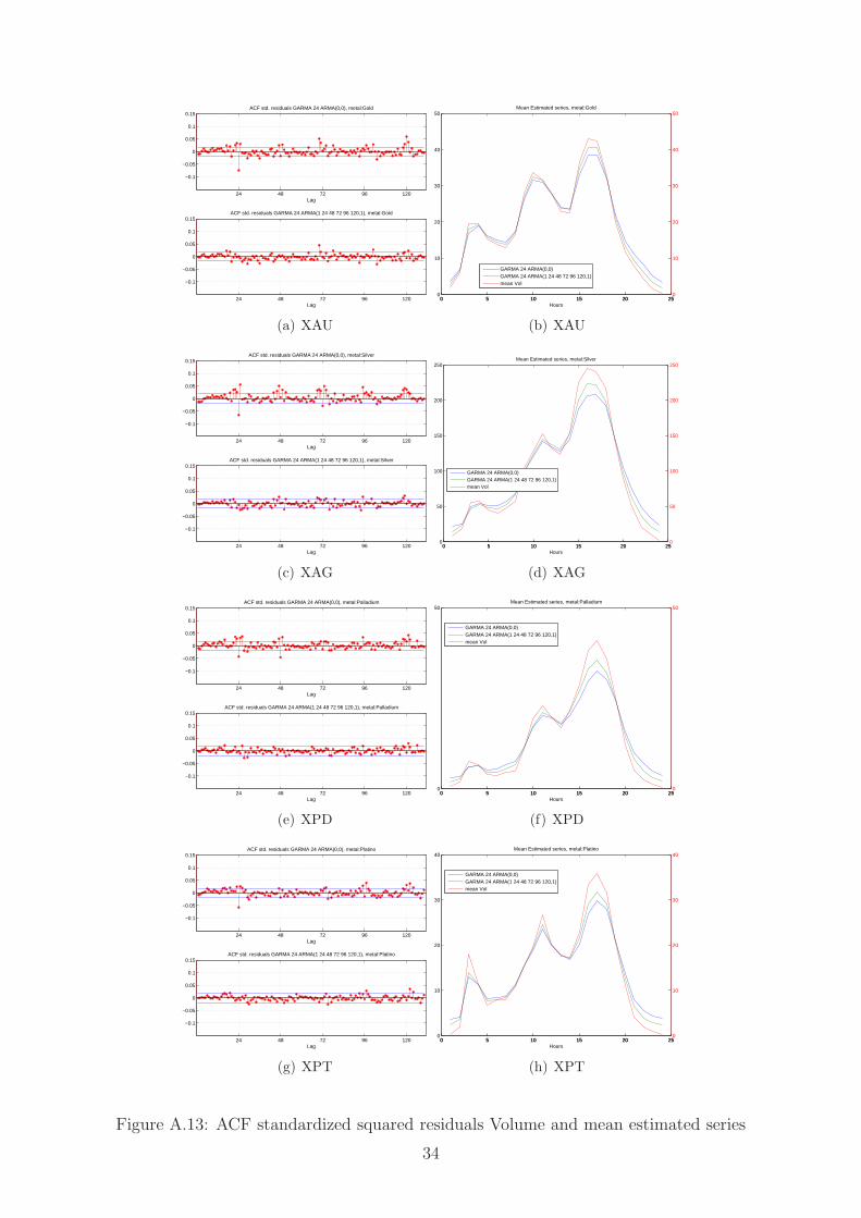
24 48 72 96 120

−0.1

−0.05

0

0.05

0.1

0.15

Lag

ACF std. residuals GARMA 24 ARMA(0,0), metal:Gold

24 48 72 96 120

−0.1

−0.05

0

0.05

0.1

0.15

Lag

ACF std. residuals GARMA 24 ARMA(1 24 48 72 96 120,1), metal:Gold

(a) XAU

0 5 10 15 20 250

10

20

30

40

50

Hours

Mean Estimated series, metal:Gold

0 5 10 15 20 250

10

20

30

40

50

GARMA 24 ARMA(0,0)GARMA 24 ARMA(1 24 48 72 96 120,1)mean Vol

(b) XAU

24 48 72 96 120

−0.1

−0.05

0

0.05

0.1

0.15

Lag

ACF std. residuals GARMA 24 ARMA(0,0), metal:Silver

24 48 72 96 120

−0.1

−0.05

0

0.05

0.1

0.15

Lag

ACF std. residuals GARMA 24 ARMA(1 24 48 72 96 120,1), metal:Silver

(c) XAG

0 5 10 15 20 250

50

100

150

200

250

Hours

Mean Estimated series, metal:Silver

0 5 10 15 20 250

50

100

150

200

250

GARMA 24 ARMA(0,0)GARMA 24 ARMA(1 24 48 72 96 120,1)mean Vol

(d) XAG

24 48 72 96 120

−0.1

−0.05

0

0.05

0.1

0.15

Lag

ACF std. residuals GARMA 24 ARMA(0,0), metal:Palladium

24 48 72 96 120

−0.1

−0.05

0

0.05

0.1

0.15

Lag

ACF std. residuals GARMA 24 ARMA(1 24 48 72 96 120,1), metal:Palladium

(e) XPD

0 5 10 15 20 250

50

Hours

Mean Estimated series, metal:Palladium

0 5 10 15 20 250

50

GARMA 24 ARMA(0,0)GARMA 24 ARMA(1 24 48 72 96 120,1)mean Vol

(f) XPD

24 48 72 96 120

−0.1

−0.05

0

0.05

0.1

0.15

Lag

ACF std. residuals GARMA 24 ARMA(0,0), metal:Platino

24 48 72 96 120

−0.1

−0.05

0

0.05

0.1

0.15

Lag

ACF std. residuals GARMA 24 ARMA(1 24 48 72 96 120,1), metal:Platino

(g) XPT

0 5 10 15 20 250

10

20

30

40

Hours

Mean Estimated series, metal:Platino

0 5 10 15 20 250

10

20

30

40

GARMA 24 ARMA(0,0)GARMA 24 ARMA(1 24 48 72 96 120,1)mean Vol

(h) XPT

Figure A.13: ACF standardized squared residuals Volume and mean estimated series

34

Table A.3: Estimation OF 2/100 ARFIMA with harmonics

XAU XAU XAG XAG XPD XPD XPT XPT

d 0.051a 0.046a 0.168a 0.163a 0.080a 0.077a 0.070a 0.071a

(0.014) (0.014) (0.025) (0.025) (0.009) (0.009) (0.009) (0.009)φ1 0.294a 0.294a 0.734a 0.724a −0.261c −0.165 −0.547b −0.616a

(0.068) (0.062) (0.046) (0.045) (0.137) (0.109) (0.255) (0.219)φ24 0.031a 0.029a 0.008 0.007 0.055a 0.054a 0.021b 0.020b

(0.008) (0.008) (0.006) (0.006) (0.009) (0.009) (0.008) (0.008)φ48 - 0.027a - 0.005 - 0.038a - −0.001

(0.008) (0.006) (0.009) (0.007)φ72 - 0.021b - 0.002 - −0.015c - −0.001

(0.008) (0.006) (0.009) (0.007)φ96 - 0.020b - 0.014b - 0.016c - −0.007

(0.008) (0.006) (0.009) (0.007)φ120 0.051a 0.048a 0.011c 0.010 −0.007 −0.007 0.004 0.005

(0.008) (0.008) (0.006) (0.006) (0.009) (0.009) (0.009) (0.008)θ1 −0.195a −0.191a −0.806a −0.794a 0.291b 0.198c 0.558b 0.624a

(0.064) (0.058) (0.033) (0.035) (0.133) (0.107) (0.245) (0.210)µ −0.827a −0.826a −0.056a −0.056a −0.051a −0.051a −0.065a −0.065a

(0.056) (0.061) (0.007) (0.007) (0.004) (0.004) (0.005) (0.005)γ1 0.587a 0.587a 0.035a 0.035a 0.037a 0.037a 0.044a 0.044a

(0.053) (0.059) (0.003) (0.003) (0.003) (0.003) (0.004) (0.004)φ1 0.453a 0.452a 0.038a 0.038a 0.044a 0.044a 0.030a 0.030a

(0.053) (0.059) (0.003) (0.003) (0.003) (0.003) (0.004) (0.004)γ2 0.309a 0.309a 0.019a 0.019a 0.018a 0.018a 0.020a 0.020a

(0.050) (0.055) (0.003) (0.003) (0.003) (0.003) (0.004) (0.004)φ2 −0.268a −0.268a −0.012a −0.012a −0.019a −0.019a −0.019a −0.019a

(0.050) (0.055) (0.003) (0.003) (0.003) (0.003) (0.004) (0.004)γ3 −0.151a −0.150a −0.002 −0.002 −0.002 −0.002 0.007c 0.007c

(0.047) (0.051) (0.003) (0.003) (0.003) (0.003) (0.003) (0.003)φ3 −0.245a −0.245a −0.016a −0.016a −0.018a −0.018a −0.029a −0.029a

(0.047) (0.051) (0.003) (0.003) (0.003) (0.003) (0.003) (0.003)γ4 0.093b 0.093c 0.002 0.002 −0.005c −0.005c −0.004 −0.004

(0.044) (0.048) (0.003) (0.003) (0.003) (0.003) (0.003) (0.003)φ4 0.237a 0.237a 0.007b 0.007b 0.008a 0.008a 0.013a 0.013a

(0.044) (0.048) (0.003) (0.003) (0.003) (0.003) (0.003) (0.003)γ5 0.017 0.017 −0.001 −0.001 −0.000 −0.000 0.006c 0.006c

(0.042) (0.045) (0.002) (0.002) (0.002) (0.003) (0.003) (0.003)φ5 −0.013 −0.013 −0.003 −0.003 0.005c 0.005c 0.011a 0.011a

(0.042) (0.045) (0.002) (0.002) (0.002) (0.003) (0.003) (0.003)σ 9.238a 9.220a 0.050a 0.050a 0.049a 0.049a 0.085a 0.085a

(0.118) (0.119) (0.000) (0.000) (0.000) (0.000) (0.001) (0.001)LLF -30063.71 -30052.31 858.8025 861.9133 1032.726 1044.071 -2263.594 -2263.024

Note: Estimation results for the OF 2/100 series for the precious metals: Gold (XAU), Silver (XAG), Palladium (XPD)and Platinum (XPT). ARFIMA models.Period 27th of December 2008 to the 30th of November 2010. Hourly series, 11880observations. LLF is the Log-likelihood function. Standard errors in bracket. ”a”, ”b” and ”c” indicate significance at the1%, 5% and 10%.

35

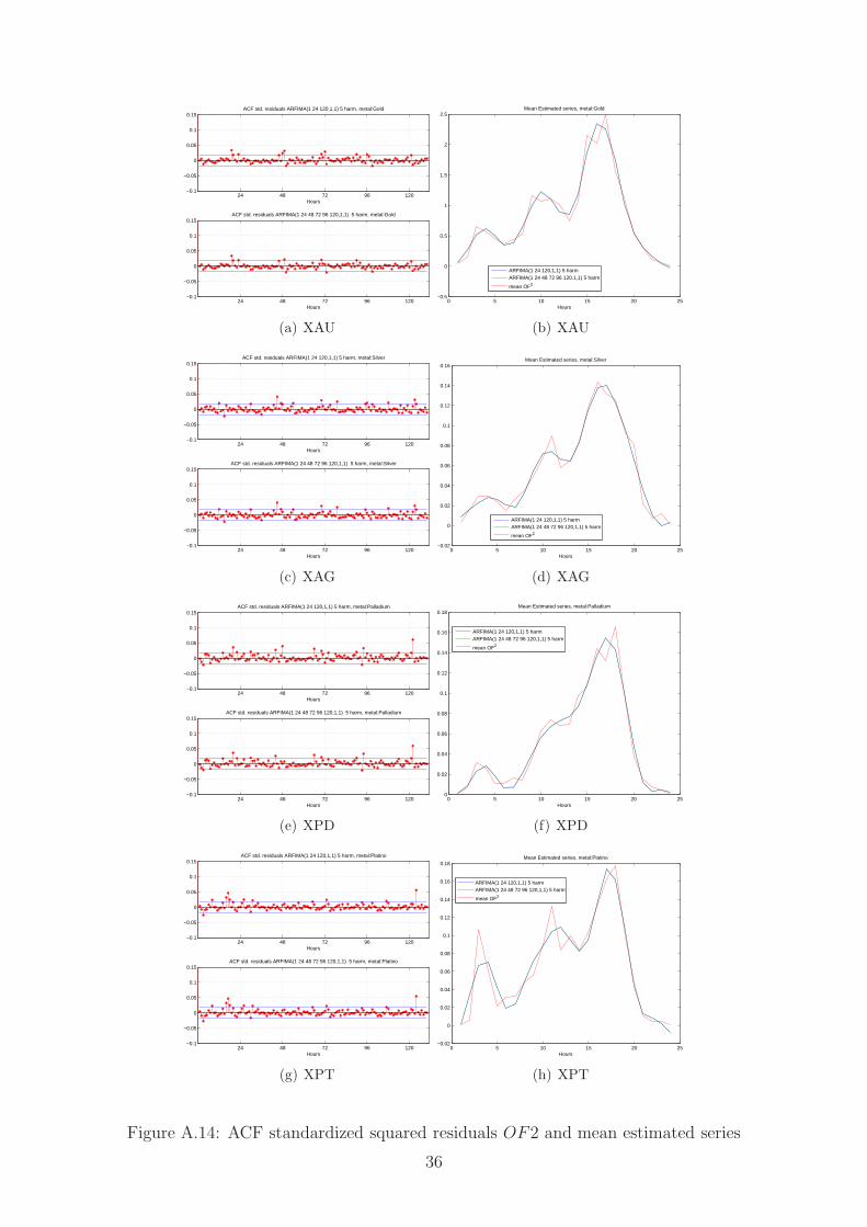
24 48 72 96 120−0.1

−0.05

0

0.05

0.1

0.15

Hours

ACF std. residuals ARFIMA(1 24 120,1,1) 5 harm, metal:Gold

24 48 72 96 120−0.1

−0.05

0

0.05

0.1

0.15

Hours

ACF std. residuals ARFIMA(1 24 48 72 96 120,1,1) 5 harm, metal:Gold

(a) XAU

0 5 10 15 20 25−0.5

0

0.5

1

1.5

2

2.5

Hours

Mean Estimated series, metal:Gold

ARFIMA(1 24 120,1,1) 5 harmARFIMA(1 24 48 72 96 120,1,1) 5 harm

mean OF2

(b) XAU

24 48 72 96 120−0.1

−0.05

0

0.05

0.1

0.15

Hours

ACF std. residuals ARFIMA(1 24 120,1,1) 5 harm, metal:Silver

24 48 72 96 120−0.1

−0.05

0

0.05

0.1

0.15

Hours

ACF std. residuals ARFIMA(1 24 48 72 96 120,1,1) 5 harm, metal:Silver

(c) XAG

0 5 10 15 20 25−0.02

0

0.02

0.04

0.06

0.08

0.1

0.12

0.14

0.16

Hours

Mean Estimated series, metal:Silver

ARFIMA(1 24 120,1,1) 5 harmARFIMA(1 24 48 72 96 120,1,1) 5 harm

mean OF2

(d) XAG

24 48 72 96 120−0.1

−0.05

0

0.05

0.1

0.15

Hours

ACF std. residuals ARFIMA(1 24 120,1,1) 5 harm, metal:Palladium

24 48 72 96 120−0.1

−0.05

0

0.05

0.1

0.15

Hours

ACF std. residuals ARFIMA(1 24 48 72 96 120,1,1) 5 harm, metal:Palladium

(e) XPD

0 5 10 15 20 250

0.02

0.04

0.06

0.08

0.1

0.12

0.14

0.16

0.18

Hours

Mean Estimated series, metal:Palladium

ARFIMA(1 24 120,1,1) 5 harmARFIMA(1 24 48 72 96 120,1,1) 5 harm

mean OF2

(f) XPD

24 48 72 96 120−0.1

−0.05

0

0.05

0.1

0.15

Hours

ACF std. residuals ARFIMA(1 24 120,1,1) 5 harm, metal:Platino

24 48 72 96 120−0.1

−0.05

0

0.05

0.1

0.15

Hours

ACF std. residuals ARFIMA(1 24 48 72 96 120,1,1) 5 harm, metal:Platino

(g) XPT

0 5 10 15 20 25−0.02

0

0.02

0.04

0.06

0.08

0.1

0.12

0.14

0.16

0.18

Hours

Mean Estimated series, metal:Platino

ARFIMA(1 24 120,1,1) 5 harmARFIMA(1 24 48 72 96 120,1,1) 5 harm

mean OF2

(h) XPT

Figure A.14: ACF standardized squared residuals OF2 and mean estimated series

36

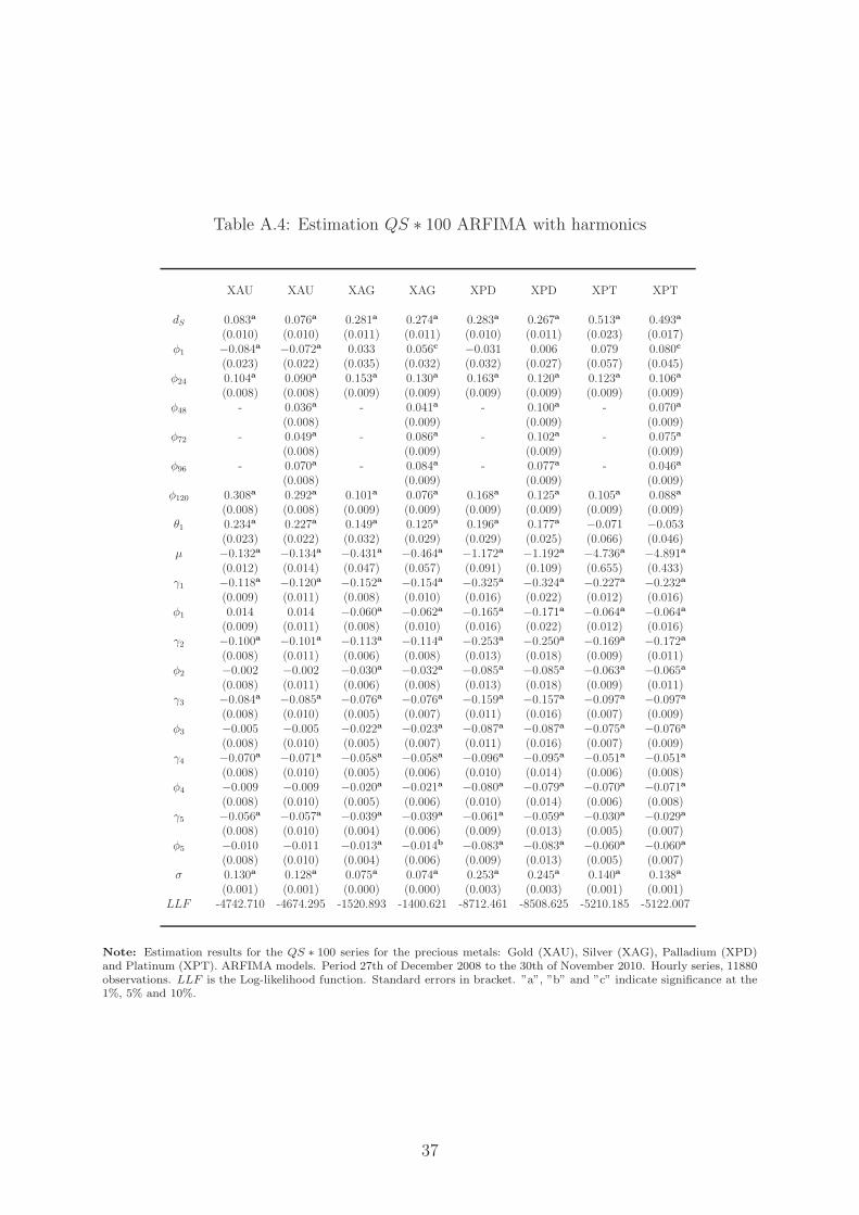
Table A.4: Estimation QS ∗ 100 ARFIMA with harmonics

XAU XAU XAG XAG XPD XPD XPT XPT

dS 0.083a 0.076a 0.281a 0.274a 0.283a 0.267a 0.513a 0.493a

(0.010) (0.010) (0.011) (0.011) (0.010) (0.011) (0.023) (0.017)φ1 −0.084a −0.072a 0.033 0.056c −0.031 0.006 0.079 0.080c

(0.023) (0.022) (0.035) (0.032) (0.032) (0.027) (0.057) (0.045)φ24 0.104a 0.090a 0.153a 0.130a 0.163a 0.120a 0.123a 0.106a

(0.008) (0.008) (0.009) (0.009) (0.009) (0.009) (0.009) (0.009)φ48 - 0.036a - 0.041a - 0.100a - 0.070a

(0.008) (0.009) (0.009) (0.009)φ72 - 0.049a - 0.086a - 0.102a - 0.075a

(0.008) (0.009) (0.009) (0.009)φ96 - 0.070a - 0.084a - 0.077a - 0.046a

(0.008) (0.009) (0.009) (0.009)φ120 0.308a 0.292a 0.101a 0.076a 0.168a 0.125a 0.105a 0.088a

(0.008) (0.008) (0.009) (0.009) (0.009) (0.009) (0.009) (0.009)θ1 0.234a 0.227a 0.149a 0.125a 0.196a 0.177a −0.071 −0.053

(0.023) (0.022) (0.032) (0.029) (0.029) (0.025) (0.066) (0.046)µ −0.132a −0.134a −0.431a −0.464a −1.172a −1.192a −4.736a −4.891a

(0.012) (0.014) (0.047) (0.057) (0.091) (0.109) (0.655) (0.433)γ1 −0.118a −0.120a −0.152a −0.154a −0.325a −0.324a −0.227a −0.232a

(0.009) (0.011) (0.008) (0.010) (0.016) (0.022) (0.012) (0.016)φ1 0.014 0.014 −0.060a −0.062a −0.165a −0.171a −0.064a −0.064a

(0.009) (0.011) (0.008) (0.010) (0.016) (0.022) (0.012) (0.016)γ2 −0.100a −0.101a −0.113a −0.114a −0.253a −0.250a −0.169a −0.172a

(0.008) (0.011) (0.006) (0.008) (0.013) (0.018) (0.009) (0.011)φ2 −0.002 −0.002 −0.030a −0.032a −0.085a −0.085a −0.063a −0.065a

(0.008) (0.011) (0.006) (0.008) (0.013) (0.018) (0.009) (0.011)γ3 −0.084a −0.085a −0.076a −0.076a −0.159a −0.157a −0.097a −0.097a

(0.008) (0.010) (0.005) (0.007) (0.011) (0.016) (0.007) (0.009)φ3 −0.005 −0.005 −0.022a −0.023a −0.087a −0.087a −0.075a −0.076a

(0.008) (0.010) (0.005) (0.007) (0.011) (0.016) (0.007) (0.009)γ4 −0.070a −0.071a −0.058a −0.058a −0.096a −0.095a −0.051a −0.051a

(0.008) (0.010) (0.005) (0.006) (0.010) (0.014) (0.006) (0.008)φ4 −0.009 −0.009 −0.020a −0.021a −0.080a −0.079a −0.070a −0.071a

(0.008) (0.010) (0.005) (0.006) (0.010) (0.014) (0.006) (0.008)γ5 −0.056a −0.057a −0.039a −0.039a −0.061a −0.059a −0.030a −0.029a

(0.008) (0.010) (0.004) (0.006) (0.009) (0.013) (0.005) (0.007)φ5 −0.010 −0.011 −0.013a −0.014b −0.083a −0.083a −0.060a −0.060a

(0.008) (0.010) (0.004) (0.006) (0.009) (0.013) (0.005) (0.007)σ 0.130a 0.128a 0.075a 0.074a 0.253a 0.245a 0.140a 0.138a

(0.001) (0.001) (0.000) (0.000) (0.003) (0.003) (0.001) (0.001)LLF -4742.710 -4674.295 -1520.893 -1400.621 -8712.461 -8508.625 -5210.185 -5122.007

Note: Estimation results for the QS ∗ 100 series for the precious metals: Gold (XAU), Silver (XAG), Palladium (XPD)and Platinum (XPT). ARFIMA models. Period 27th of December 2008 to the 30th of November 2010. Hourly series, 11880observations. LLF is the Log-likelihood function. Standard errors in bracket. ”a”, ”b” and ”c” indicate significance at the1%, 5% and 10%.

37

24 48 72 96 120−0.1

−0.05

0

0.05

0.1

0.15

Hours

ACF std. residuals ARFIMA(1 24 120,1,1) 5 harm, metal:Gold

24 48 72 96 120−0.1

−0.05

0

0.05

0.1

0.15

Hours

ACF std. residuals ARFIMA(1 24 48 72 96 120,1,1) 5 harm, metal:Gold

(a) XAU

0 5 10 15 20 250

0.1

0.2

0.3

0.4

0.5

0.6

0.7

0.8

Hours

Mean Estimated series, metal:Gold

ARFIMA(1 24 120,1,1) 5 harmARFIMA(1 24 48 72 96 120,1,1) 5 harmmean QS

(b) XAU

24 48 72 96 120−0.1

−0.05

0

0.05

0.1

0.15

Hours

ACF std. residuals ARFIMA(1 24 120,1,1) 5 harm, metal:Silver

24 48 72 96 120−0.1

−0.05

0

0.05

0.1

0.15

Hours

ACF std. residuals ARFIMA(1 24 48 72 96 120,1,1) 5 harm, metal:Silver

(c) XAG

0 5 10 15 20 250.2

0.3

0.4

0.5

0.6

0.7

0.8

0.9

1

Hours

Mean Estimated series, metal:Silver

ARFIMA(1 24 120,1,1) 5 harmARFIMA(1 24 48 72 96 120,1,1) 5 harmmean QS

(d) XAG

24 48 72 96 120−0.1

−0.05

0

0.05

0.1

0.15

Hours

ACF std. residuals ARFIMA(1 24 120,1,1) 5 harm, metal:Palladium

24 48 72 96 120−0.1

−0.05

0

0.05

0.1

0.15

Hours

ACF std. residuals ARFIMA(1 24 48 72 96 120,1,1) 5 harm, metal:Palladium

(e) XPD

0 5 10 15 20 25

0.8

1

1.2

1.4

1.6

1.8

2

2.2

Hours

Mean Estimated series, metal:Palladium

ARFIMA(1 24 120,1,1) 5 harmARFIMA(1 24 48 72 96 120,1,1) 5 harmmean QS

(f) XPD

24 48 72 96 120−0.1

−0.05

0

0.05

0.1

0.15

Hours

ACF std. residuals ARFIMA(1 24 120,1,1) 5 harm, metal:Platino

24 48 72 96 120−0.1

−0.05

0

0.05

0.1

0.15

Hours

ACF std. residuals ARFIMA(1 24 48 72 96 120,1,1) 5 harm, metal:Platino

(g) XPT

0 5 10 15 20 25

0.4

0.5

0.6

0.7

0.8

0.9

1

1.1

1.2

1.3

Hours

Mean Estimated series, metal:Platino

ARFIMA(1 24 120,1,1) 5 harmARFIMA(1 24 48 72 96 120,1,1) 5 harmmean QS

(h) XPT

Figure A.15: ACF standardized squared residuals QS and mean estimated series

38