G. Cowan Lectures on Statistical Data Analysis Lecture 7 page 1 Statistical Data Analysis: Lecture 7 1Probability, Bayes’ theorem 2Random variables and

G. Cowan Lectures on Statistical Data Analysis Lecture 7 page 1

Statistical Data Analysis: Lecture 7

1 Probability, Bayes’ theorem2 Random variables and probability densities3 Expectation values, error propagation4 Catalogue of pdfs5 The Monte Carlo method6 Statistical tests: general concepts7 Test statistics, multivariate methods8 Goodness-of-fit tests9 Parameter estimation, maximum likelihood10 More maximum likelihood11 Method of least squares12 Interval estimation, setting limits13 Nuisance parameters, systematic uncertainties14 Examples of Bayesian approach


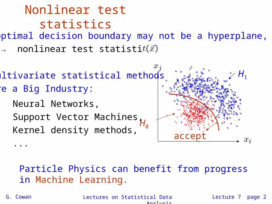
Nonlinear test statistics

The optimal decision boundary may not be a hyperplane,

→ nonlinear test statistic

accept

H0

H1Multivariate statistical methods

are a Big Industry:

Particle Physics can benefit from progress in Machine Learning.

Neural Networks,

Support Vector Machines,

Kernel density methods,

...


Introduction to neural networks

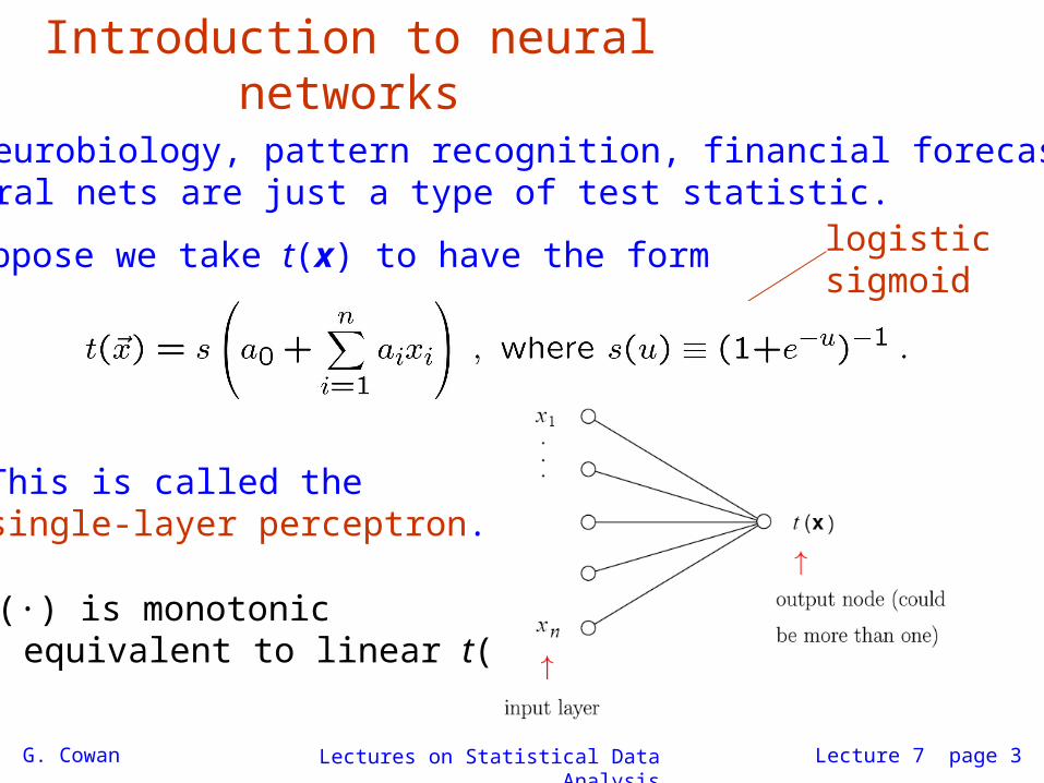
Used in neurobiology, pattern recognition, financial forecasting, ...Here, neural nets are just a type of test statistic.

Suppose we take t(x) to have the form logisticsigmoid

This is called the single-layer perceptron.

s(·) is monotonic → equivalent to linear t(x)


The multi-layer perceptron

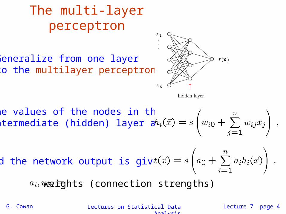
Generalize from one layer to the multilayer perceptron:

The values of the nodes in the intermediate (hidden) layer are

and the network output is given by

weights (connection strengths)


Neural network discussion

Easy to generalize to arbitrary number of layers.

Feed-forward net: values of a node depend only on earlier layers,usually only on previous layer (“network architecture”).

More nodes → neural net gets closer to optimal t(x), butmore parameters need to be determined.

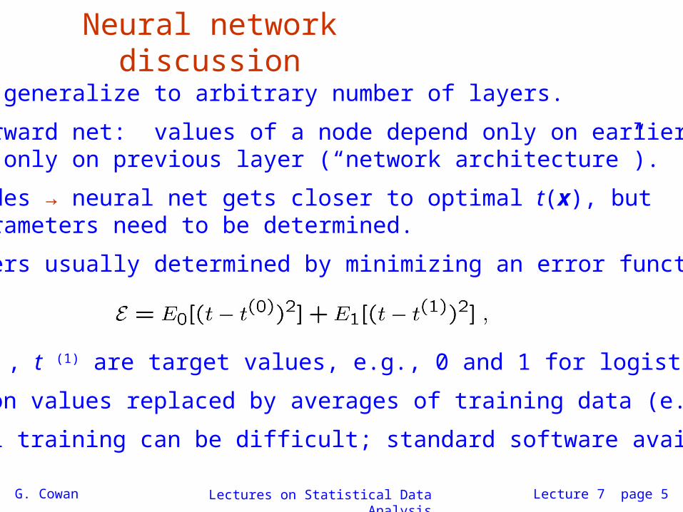
Parameters usually determined by minimizing an error function,

where t (0) , t (1) are target values, e.g., 0 and 1 for logistic sigmoid.

Expectation values replaced by averages of training data (e.g. MC).

In general training can be difficult; standard software available.


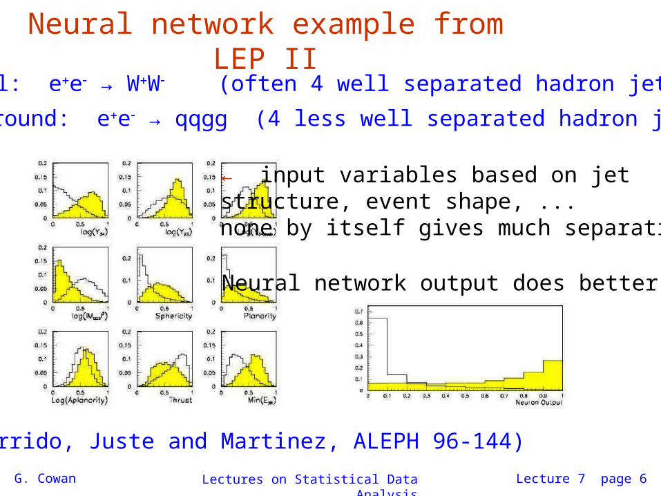
Neural network example from LEP IISignal: ee → WW (often 4 well separated hadron jets)

Background: ee → qqgg (4 less well separated hadron jets)

← input variables based on jetstructure, event shape, ...none by itself gives much separation.

Neural network output does better...

(Garrido, Juste and Martinez, ALEPH 96-144)

G. Cowan Statistical methods for particle physics page 7

Some issues with neural networksIn the example with WW events, goal was to select these eventsso as to study properties of the W boson.

Needed to avoid using input variables correlated to theproperties we eventually wanted to study (not trivial).

In principle a single hidden layer with an sufficiently large number ofnodes can approximate arbitrarily well the optimal test variable (likelihoodratio).

Usually start with relatively small number of nodes and increaseuntil misclassification rate on validation data sample ceasesto decrease.

Usually MC training data is cheap -- problems with getting stuck in local minima, overtraining, etc., less important than concerns of systematic differences between the training data and Nature, and concerns aboutthe ease of interpretation of the output.


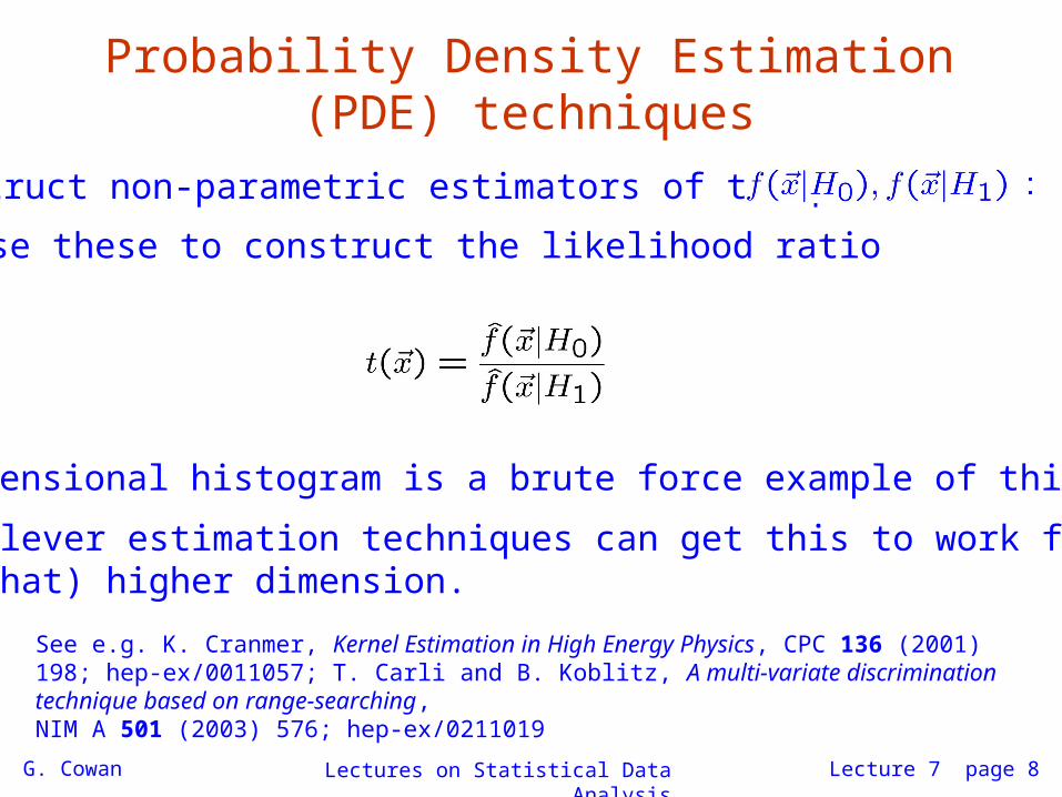
Probability Density Estimation (PDE) techniques

See e.g. K. Cranmer, Kernel Estimation in High Energy Physics, CPC 136 (2001) 198; hep-ex/0011057; T. Carli and B. Koblitz, A multi-variate discrimination technique based on range-searching, NIM A 501 (2003) 576; hep-ex/0211019

Construct non-parametric estimators of the pdfs

and use these to construct the likelihood ratio

(n-dimensional histogram is a brute force example of this.)

More clever estimation techniques can get this to work for(somewhat) higher dimension.


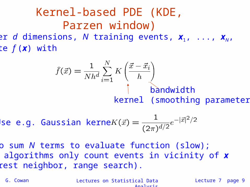
Kernel-based PDE (KDE, Parzen window)

Consider d dimensions, N training events, x1, ..., xN, estimate f (x) with

Use e.g. Gaussian kernel:

kernelbandwidth (smoothing parameter)

Need to sum N terms to evaluate function (slow); faster algorithms only count events in vicinity of x (k-nearest neighbor, range search).


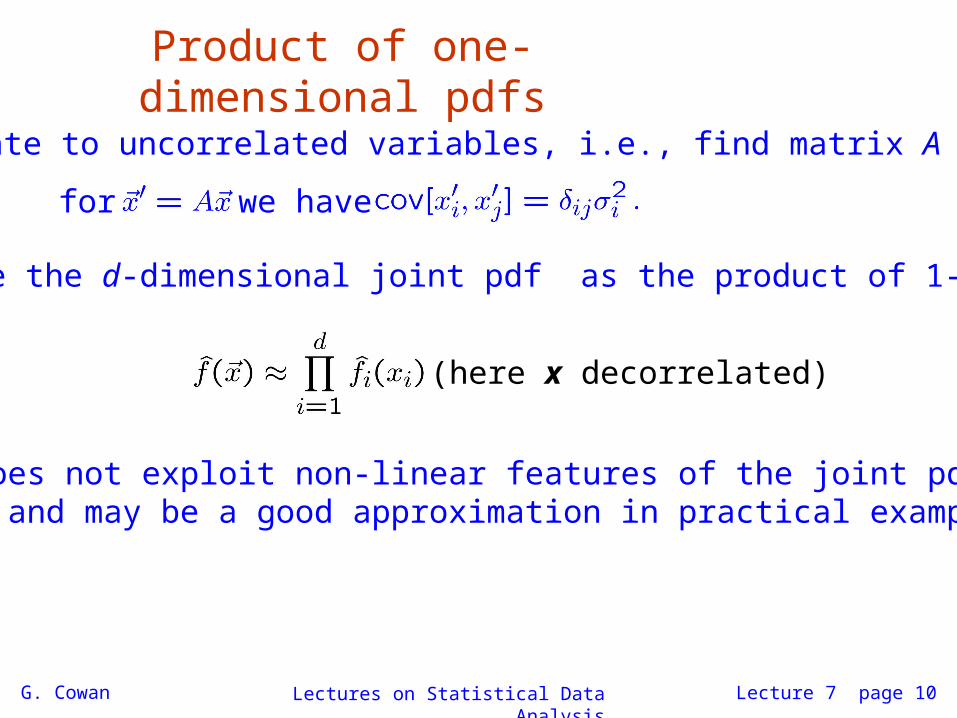
Product of one-dimensional pdfs

First rotate to uncorrelated variables, i.e., find matrix A such that

for we have

Estimate the d-dimensional joint pdf as the product of 1-d pdfs,

(here x decorrelated)

This does not exploit non-linear features of the joint pdf, butsimple and may be a good approximation in practical examples.


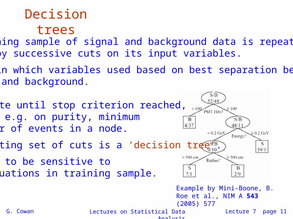
Decision trees

A training sample of signal and background data is repeatedlysplit by successive cuts on its input variables.

Order in which variables used based on best separation betweensignal and background.

Example by Mini-Boone, B. Roe et al., NIM A 543 (2005) 577

Iterate until stop criterion reached,based e.g. on purity, minimumnumber of events in a node.

Resulting set of cuts is a ‘decision tree’.

Tends to be sensitive to fluctuations in training sample.


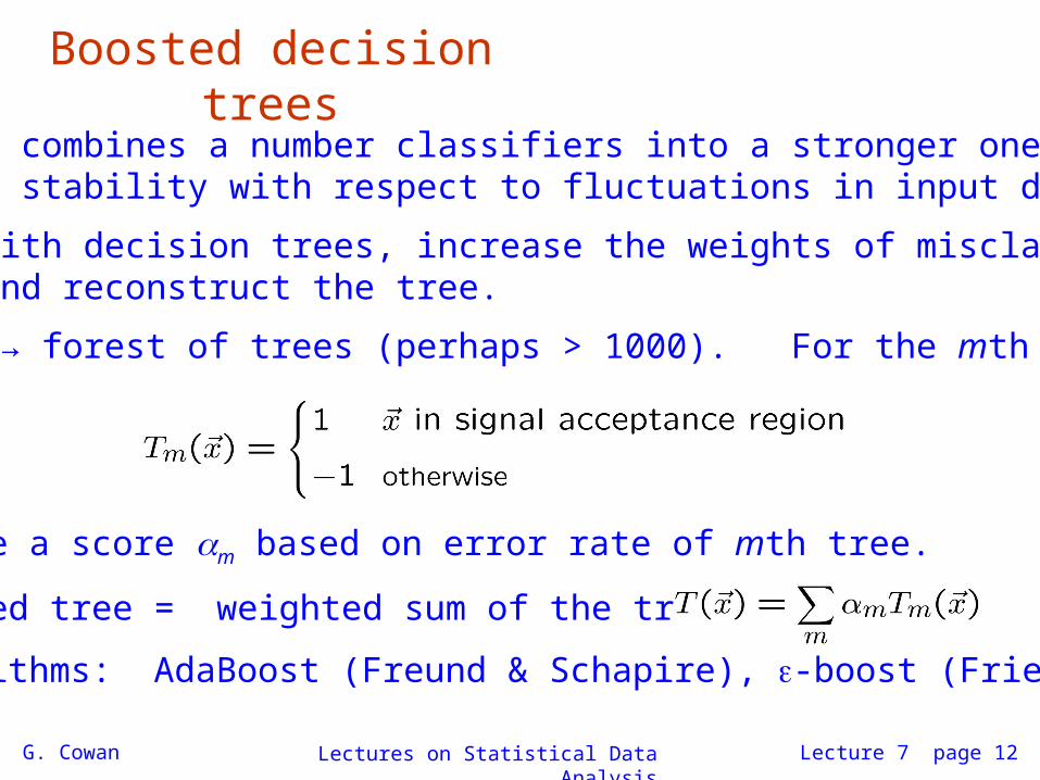
Boosted decision trees

Boosting combines a number classifiers into a stronger one; improves stability with respect to fluctuations in input data.

To use with decision trees, increase the weights of misclassifiedevents and reconstruct the tree.

Iterate → forest of trees (perhaps > 1000). For the mth tree,

Define a score m based on error rate of mth tree.

Boosted tree = weighted sum of the trees:

Algorithms: AdaBoost (Freund & Schapire), -boost (Friedman).


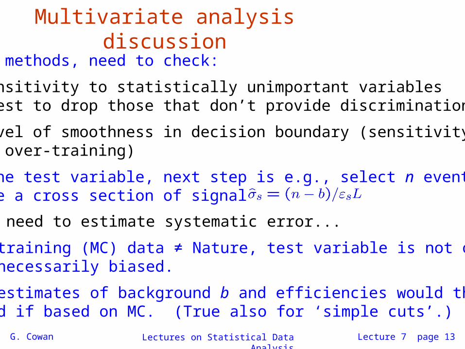
For all methods, need to check:

Sensitivity to statistically unimportant variables(best to drop those that don’t provide discrimination);

Level of smoothness in decision boundary (sensitivityto over-training)

Given the test variable, next step is e.g., select n events andestimate a cross section of signal:

Multivariate analysis discussion

Now need to estimate systematic error...

If e.g. training (MC) data ≠ Nature, test variable is not optimal,but not necessarily biased.

But our estimates of background b and efficiencies would then be biased if based on MC. (True also for ‘simple cuts’.)

G. Cowan page 14

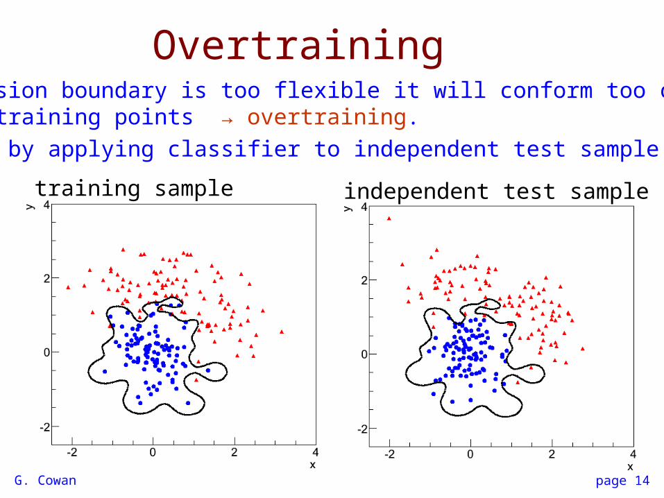
Overtraining

training sample independent test sample

If decision boundary is too flexible it will conform too closelyto the training points → overtraining.

Monitor by applying classifier to independent test sample.

G. Cowan page 15

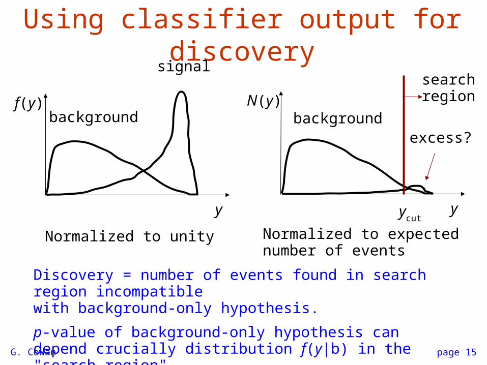
Using classifier output for discovery

y

f(y)

y

N(y)

Normalized to unity Normalized to expected number of events

excess?

signal

background background

searchregion

Discovery = number of events found in search region incompatiblewith background-only hypothesis.

p-value of background-only hypothesis can depend crucially distribution f(y|b) in the "search region".

ycut

G. Cowan SUSSP65, St Andrews, 16-29 August 2009 / Statistical Methods 3

page 16

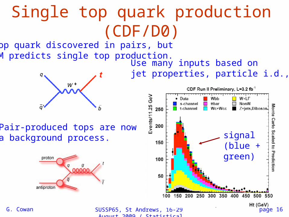
Single top quark production (CDF/D0)Top quark discovered in pairs, butSM predicts single top production.

Use many inputs based on jet properties, particle i.d., ...

signal(blue +green)

Pair-produced tops are now a background process.


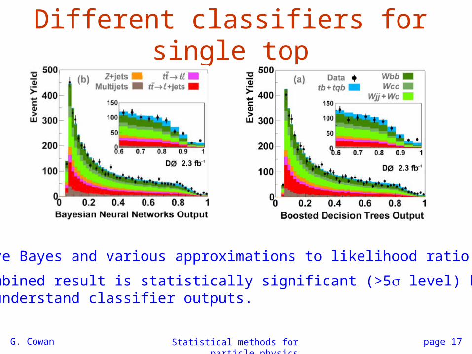
Different classifiers for single top

Also Naive Bayes and various approximations to likelihood ratio,....

Final combined result is statistically significant (>5 level) but not easy to understand classifier outputs.



Comparing multivariate methods (TMVA)

Choose the best one!



Wrapping up lecture 7

We looked at statistical tests and related issues:discriminate between event types (hypotheses),determine selection efficiency, sample purity, etc.

Some modern (and less modern) methods were mentioned:Fisher discriminants, neural networks,PDE, KDE, decision trees, ...

Next we will talk about goodness-of-fit tests:p-value expresses level of agreement between data and hypothesis

Documents

G. Cowan Lectures on Statistical Data Analysis Lecture 7 page 1 Statistical Data Analysis: Lecture 7 1Probability, Bayes’ theorem 2Random variables and