BAU Journal - Science and Technology BAU Journal - Science and Technology

Volume 1 Issue 2 ISSN: 2706-784X Article 2

June 2020

FUZZY LOGIC VELOCITY OPTIMIZATION OF AUTONOMOUS FUZZY LOGIC VELOCITY OPTIMIZATION OF AUTONOMOUS

VEHICLES BASED ON ROAD BUMP GEOMETRY VEHICLES BASED ON ROAD BUMP GEOMETRY

Yassine Zein Graduate Engineer, Faculty of Engineering, Beirut Arab University, Beirut, Lebanon, yassine.zein@hotmail.com

Mohamad Darwiche Assistant Professor, Faculty of Engineering, Beirut Arab University, Beirut, Lebanon, m.darwich@bau.edu.lb

Follow this and additional works at: https://digitalcommons.bau.edu.lb/stjournal

Part of the Architecture Commons, Business Commons, Engineering Commons, and the Physical

Sciences and Mathematics Commons

Recommended Citation Recommended Citation Zein, Yassine and Darwiche, Mohamad (2020) "FUZZY LOGIC VELOCITY OPTIMIZATION OF AUTONOMOUS VEHICLES BASED ON ROAD BUMP GEOMETRY," BAU Journal - Science and Technology: Vol. 1 : Iss. 2 , Article 2. Available at: https://digitalcommons.bau.edu.lb/stjournal/vol1/iss2/2

This Article is brought to you for free and open access by Digital Commons @ BAU. It has been accepted for inclusion in BAU Journal - Science and Technology by an authorized editor of Digital Commons @ BAU. For more information, please contact ibtihal@bau.edu.lb.

FUZZY LOGIC VELOCITY OPTIMIZATION OF AUTONOMOUS VEHICLES BASED ON FUZZY LOGIC VELOCITY OPTIMIZATION OF AUTONOMOUS VEHICLES BASED ON ROAD BUMP GEOMETRY ROAD BUMP GEOMETRY

Abstract Abstract In today’s world of fast developing technologies, semi-autonomous vehicles are becoming a common sight and increasing in numbers. Some feature autopilot systems that drive the vehicle without any intervention from the driver in certain situations or warn the driver of dangers ahead. A fully autonomous vehicle is yet to come due to old fashioned road infrastructures that would convey challenging scenarios for it. From speed bumps and traffic lights to road lanes and warning signs, current autopilot systems will have to cope with all. A system that ensures safe crossing of speed bumps when in autopilot mode is discussed in this paper. Crossing a speed bump at high speeds may result in loss of control, suspension failure, onboard cargo damage, and/or compromised passenger comfort. The proposed system can detect a speed bump from a distance, calculate the suitable crossing speed by studying vertical acceleration disturbances, and apply the brakes automatically using a Fuzzy Logic Controller (FLC) to reduce the speed before the car reaches the speed bump.

Keywords Keywords Fuzzy logic control, autonomous vehicles, ride comfort, bump detection

This article is available in BAU Journal - Science and Technology: https://digitalcommons.bau.edu.lb/stjournal/vol1/iss2/2

1. INTRODUCTION Since the dawn of transportation, engineers gave a great interest in improving the ride

quality and drivability of vehicles. After over 100 years of the invention of the internal combustion

engine which paved the way to the modern vehicles as we know them today, designers are still

developing new systems for vehicles to further cope with varying road conditions, optimize

passenger comfort, increase safety, and improve efficiency. This would not be possible without

the introduction of electronic systems to vehicles. Automated vehicle systems optimize the work

of mechanical systems by eliminating as much as possible any intervention from humans. This

guarantees near optimum response of any system anytime and at any situation. Engines became

more fuel efficient and more powerful at the same time with the help of Electronic Computer Units

(ECU) (HowStuffWorks.com, 1). Gearboxes, assisted by a computer, can select the optimum gear

depending on the driving situation yielding better power transmission efficiency and performance.

Automated suspension systems increase dampness to manage speed bumps and potholes in normal

driving, firm up the controls for the driver in race mode, and manage extreme driving situations

in case of harsh weather conditions and off-road expeditions.

The main problem facing autonomous vehicles of our time is that the technology behind

them is developing faster than the road infrastructure. Roads are still based on old-car technologies

driven entirely by humans where traffic lights are mandatory to maintain safe intersections, lane

lines are paved to keep a distance from other vehicles, and speed bumps are installed to slow down

vehicles on certain roads. All of these road aids will be dispensed when all vehicles become fully

autonomous. Until then, current autopilot systems will have to cope with these conditions and

adjust to them.

This paper focuses on one of these conditions which is speed bumps. If not tackled at a

certain speed, speed bumps or humps can have serious consequences on the vehicle’s mechanicals,

passengers, and/or onboard cargo as mentioned by R. Janczur (Janczur, 2012). The system

proposed in this paper addresses this issue by detecting the speed bump from a distance and

reducing the possibly high traveling speed automatically to avoid damage or lose control. The

system calculates the suitable traveling speed that should be maintained whilst crossing the

detected speed bump so that the suspension system effectively provides a safe and comfortable

ride at all times. This also means that manufacturers could cut costs of packaging by transporting

these products in a state of the art vehicle that has this system which reduces road vibrations and

the negative effects of speed bumps.

The proposed system required two main fields of research: obstacle detection and automatic

speed control. The system in this work was based on the ability of the vehicle to detect a speed

bump along with its dimensions ahead of time. This enables the vehicle then to act autonomously

and reduce the vehicle’s speed before reaching the speed bump. In order to detect a speed bump

before reaching it, a sensory system was needed. Since this work was intended to study control

and modeling methods only, a brief literature review related to similar systems that might work to

detect a speed bump before reaching it was presented in the following lines instead of a detailed

study on the matter.

A system proposed by (Wen, 2008), uses the data from an Inertial Measurement Unit

(IMU) to detect road roughness. The system comprised by (Devapriya, Babu, & Srihari, 2016)

uses Gaussian filtering and Median filtering to process images of the road ahead to detect speed

bumps. This technique was conceived after the failure of sensors and accelerometers to efficiently

detect the speed bumps’ dimensions (Eriksson, et al., 2008). A simpler approach adopted by

(Madli, Hebbar, Pattar, & Golla, 2015) uses ultrasonic proximity sensors and GPS to locate and

determine the dimensions of a speed bump. For this arrangement to work efficiently, it requires

uninterrupted connection to GPS satellites which is not always the case in certain areas due to

environmental and security issues (Gordon, 2013). A preposition presented by S. Ramesh et al.

(S.Ramesh, Ranjan, Mukherjee, & Chaudhuri, 2012) uses a front mounted laser beam to detect

obstacles ahead. The laser beam bounces off any object in front and bounces back to a sensor.

Then the distance from the vehicle to the obstacle can be determined.

However, this setup requires supplementary aid from another system to determine whether

this obstacle is a bump or not as well as determine its height.

1

Zein and Darwiche: FUZZY LOGIC VELOCITY OPTIMIZATION OF AUTONOMOUS VEHICLES BASED ON

Published by Digital Commons @ BAU, 2020

An alternative preposition uses a camera mounted on the nose of the vehicle to view the

road ahead. A camera can provide colored and textured-base images that are virtually similar to

the real life view (Wei, Ball, & Anderson, 2018). With the help of processing methods such as

deep learning (DL) (Redmon, Divvala, Girshick, & Farhadi, 2016), these images can be analyzed

to detect specific objects in them and determine their nature both accurately and quickly (Szegedy,

Reed, Erhan, Anguelov, & Ioffe, 2014). But the downside with using a camera is the inability of

it functioning perfectly in the night and incidents of bad weather.

Another method uses a LIDAR detector to generate a 3D model of the vehicle’s surrounding

environment as shown in Fig. 1. The outstanding angular resolution and accuracy characteristics

of LIDAR coupled to its good detection performance in a wide range of incidence angles and

weather conditions, provide an ideal solution in collision avoidance systems (Sabatini, Gardi, &

Richardson, 2014) (Lin, Chen, Su, & Chen, 2014). This can be used as is to detect speed bumps

and referring to the LIDAR’s coordinate system, the dimensions of the bump can be determined

as well as the distance to reach it. The downside with LIDAR is that it cannot create a colored

image thus probably missing small speed bumps which are often striped in yellow or white.

Fig.1: LIDAR image of a road (Sharma, 2019)

A fusion of camera and LIDAR in a collision avoidance system by P. Wei et al. (Wei, Ball,

& Anderson, 2018) utilized the advantages of both and eliminated their disadvantages. The

LIDAR signals are processed to give the locations of objects as a distance in meters. While the

camera images are processed to report detection of certain objects ahead. The fusion of data

coming from both sensors creating robust detection of objects. In the speed bump application, this

system serves all needs. It can unmistakably detect a speed bump and provide the proposed system

with the necessary bump dimensions and distances.

The detection of the speed bump before reaching it enables the autopilot to reduce the high

traveling speed avoiding mishaps. From this, the field of automatic speed control was studied. The

most common speed control system is the cruise control that can keep the vehicle at a constant

speed and reduce the burden on the driver (Miyata, et al., 2010). A longitudinal collision avoidance

system uses adaptive cruise control to avoid any collision (Moon, Yi, & Kang, 2008). With the

use of radar or LIDAR sensors, the system can automatically adjust the vehicle’s speed to maintain

a safe distance from other vehicles by automatically applying the brakes, decreasing throttle, or

reducing gear ratios (Milanés, et al., 2014). This automatic response requires control methods such

as fuzzy control and Proportional-Integral-Derivative (PID) control (Pan, Bao, Pan, & Xu, 2016).

(Trebli-Olennu, Dolan, & Khosla, 2001) applied a fuzzy controller to the throttle of an all-terrain

vehicle in order to maintain a constant speed at hill climbs. A system proposed by (Aleksendrić,

Jakovljević, & Ćirović, 2012) uses a PID controller that takes a velocity set point and calculate

the necessary force to be applied to the brake pads.

2

BAU Journal - Science and Technology, Vol. 1, Iss. 2 [2020], Art. 2

https://digitalcommons.bau.edu.lb/stjournal/vol1/iss2/2

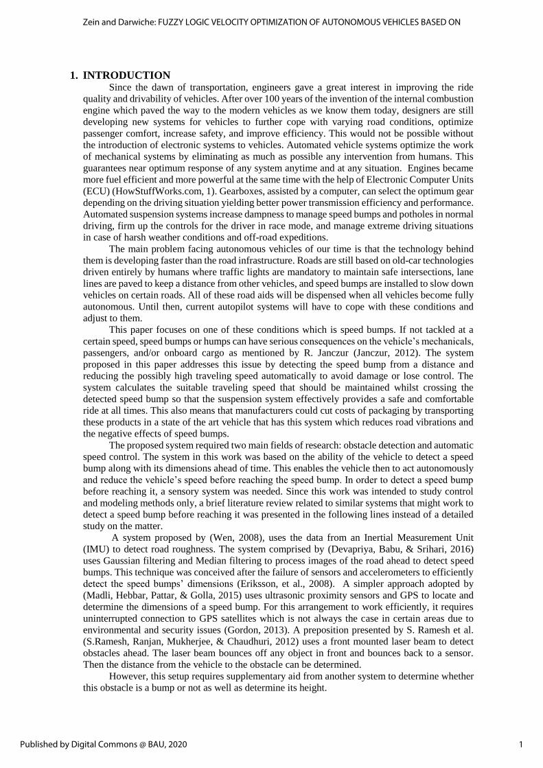
2. PROPOSED DESIGN In order to address the problem stated in the previous section, an original system was

modeled using Simulink and Matlab. The main goal was to achieve a safe and comfortable

crossing of speed bumps. This was done by a process shown in Fig.2.First the bump has to be

detected by a sensory system in order to initiate the process. Then the system generates a soft

profile of the detected speed bump in order to simulate the reaction of the suspension system to it.

The studied parameter here is the vertical acceleration which affects the ride quality of the vehicle.

After that, the velocity analyzer calculates a suitable traveling velocity that maintains the safety

and comfort standards. The vehicle may be traveling at a faster speed than the calculated suitable

one. So the brakes are to be automatically applied in order to reduce the speed before reaching the

bump using a Fuzzy Logic Controller (FLC). In this way, the bump will be crossed by the vehicle

at the calculated suitable speed and thus providing an ultimate ride quality at all times.

Fig.2: Autonomous bump crossing system process

2.1 Bump Generator After the speed bump is detected, the bump should be generated to be introduced to the

suspension model as a disturbance. The bump disturbance is in the form of a plot between the

bump vertical displacement 𝑦𝑟𝑜𝑎𝑑 and time t as the suspension model requires as an input

disturbance a plot of the road height versus time. Using this plot, the suspension model can

simulate the vertical acceleration at every instance knowing the road height at every point in

time. The total time of this disturbance is the time it takes the vehicle to cross the bump

completely. This time relies directly on the constant velocity of the vehicle while crossing the

bump. The velocity is assumed at first and the bump disturbance is generated accordingly. If

this velocity yielded low values of vertical acceleration, it is then incremented and the vertical

acceleration reassessed until the latter satisfies vertical acceleration constraints. This method

of incrementing the velocity and assessing the vertical acceleration values was used since

there is no linear equation that relates the vertical acceleration and the traveling velocity of

the vehicle. Instead, the vertical acceleration relies directly on the road height at every

instance of time in the form of a differential equation. So it was unfeasible to calculate the

vertical acceleration at every instance directly from the linear traveling velocity. The

plausible method was to generate the speed bump as a plot of 𝑦𝑟𝑜𝑎𝑑 versus time where the

total time to cross the bumps is the period 𝑇 calculated directly from the traveling velocity.

In order to generate the bump disturbance plot, the bump is approximated to be a half

sine wave with its amplitude being the height of the bump 𝐻 and its width being double the

height detected by the sensory system. Its period 𝑇 is equal to the perimeter of the bump

divided by the vehicle’s traveling velocity 𝑣 as shown in Eq. (1).

Eq. (1) 𝑇(𝑠) =

2𝜋 ∗ 𝐻(𝑚)

𝑣(𝑚/𝑠)

The bump disturbance equation for a half sine wave then is presented in Eq. (2) where

𝑦𝑟𝑜𝑎𝑑 is the vertical displacement of the road.

Eq. (2) 𝑦𝑟𝑜𝑎𝑑(𝑚) = 𝐻 ∗ sin (𝜋𝑓 ∗ 𝑡)

The road vertical displacement 𝑦𝑟𝑜𝑎𝑑 and its rate of change 𝑦𝑟𝑜𝑎𝑑̇ are then used as a

disturbance for the stationary suspension system. There is no sprung mass vertical

acceleration before reaching the bump as the vehicle is supposed to be moving on a smooth

surface. Eq. (1) and Eq. (2) were introduced to a Simulink model to be used as inputs to the

suspension model.

3

Zein and Darwiche: FUZZY LOGIC VELOCITY OPTIMIZATION OF AUTONOMOUS VEHICLES BASED ON

Published by Digital Commons @ BAU, 2020

2.2 Suspension Model In order to determine the effect of the traveling velocity on the suspension system of a

vehicle, this system must be modeled first. In this simulation, a quarter car model is used

based on an existing work (Kanjanavapastit & Thitinaruemit, 2012). The quarter car model

considers the movement of a single wheel in the vertical direction. It accounts for the

characteristics of the suspension system shown in Fig. 3 from the dampness of the shock

absorbers 𝐵𝑠 and tires 𝐵𝑡, the sprung 𝑚𝑠 and unsprung masses 𝑚𝑢𝑠, and the stiffness of the

spring 𝐾𝑠 and tires 𝐾𝑡 to determine the effect of road disturbances. This disturbance generates

vertical acceleration which is the parameter related to the direct effect of the bump on the

vehicle. As the maximum amplitude of the vertical acceleration increases, then the ride is

considered more uncomfortable and dangerous. Du and Ds are the displacements when the

springs of unsprung mass and sprung mass are compressed respectively. The associated

vertical velocities are vu and vs respectively.

Fig.3: Quarter car model (Kanjanavapastit & Thitinaruemit, 2012)

According to Newton’s second law, the sum of all forces is equal to the product of the

mass 𝒎 and acceleration 𝒂. From this, two equations were generated; one for the unsprung

mass and the other for the sprung mass.

Eq. (3) ∑𝐹 − 𝑚𝑢𝑠 ∗𝑑2𝐷𝑢

𝑑𝑡2= 0

Eq. (4) ∑𝐹 − 𝑚𝑠 ∗

𝑑2𝐷𝑢

𝑑𝑡2= 0

Substituting the forces in Eq. (3) and Eq. (4) gives Eq. (5) and Eq. (6) respectively.

Eq. (5) 𝐵𝑡(𝑦𝑟𝑜𝑎𝑑̇ − 𝐷�̇�) + 𝐾𝑡(𝑦𝑟𝑜𝑎𝑑 − 𝐷𝑢) − 𝐵𝑠(𝐷�̇� − 𝐷�̇�) − 𝐾𝑠(𝐷𝑢 − 𝐷𝑠) − 𝑚𝑢𝑠 ∗ 𝐷�̈� = 0

Eq. (6) 𝐵𝑠(𝐷�̇� − 𝐷�̇�) + 𝐾𝑠(𝐷𝑢 − 𝐷𝑠) − 𝑚𝑠 ∗ 𝐷�̈� = 0

Eq. (5) and Eq. (6) are the two differential equations that were used to construct a block

diagram on Simulink. They were used to calculate the vertical acceleration 𝐷�̈� which is the

main parameter considered to obtain the optimum bump crossing situation.

4

BAU Journal - Science and Technology, Vol. 1, Iss. 2 [2020], Art. 2

https://digitalcommons.bau.edu.lb/stjournal/vol1/iss2/2

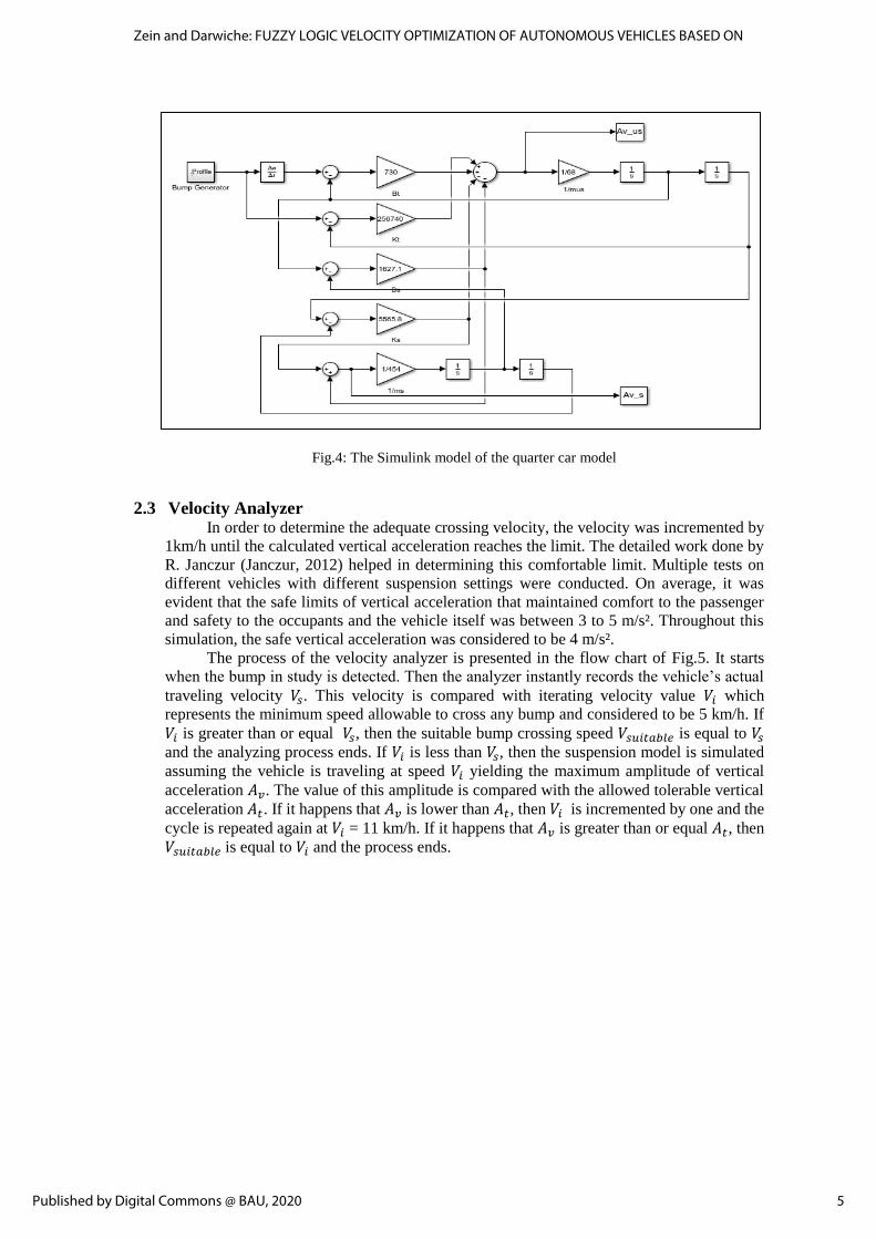
Fig.4: The Simulink model of the quarter car model

2.3 Velocity Analyzer In order to determine the adequate crossing velocity, the velocity was incremented by

1km/h until the calculated vertical acceleration reaches the limit. The detailed work done by

R. Janczur (Janczur, 2012) helped in determining this comfortable limit. Multiple tests on

different vehicles with different suspension settings were conducted. On average, it was

evident that the safe limits of vertical acceleration that maintained comfort to the passenger

and safety to the occupants and the vehicle itself was between 3 to 5 m/s². Throughout this

simulation, the safe vertical acceleration was considered to be 4 m/s².

The process of the velocity analyzer is presented in the flow chart of Fig.5. It starts

when the bump in study is detected. Then the analyzer instantly records the vehicle’s actual

traveling velocity 𝑉𝑠. This velocity is compared with iterating velocity value 𝑉𝑖 which

represents the minimum speed allowable to cross any bump and considered to be 5 km/h. If

𝑉𝑖 is greater than or equal 𝑉𝑠, then the suitable bump crossing speed 𝑉𝑠𝑢𝑖𝑡𝑎𝑏𝑙𝑒 is equal to 𝑉𝑠

and the analyzing process ends. If 𝑉𝑖 is less than 𝑉𝑠, then the suspension model is simulated

assuming the vehicle is traveling at speed 𝑉𝑖 yielding the maximum amplitude of vertical

acceleration 𝐴𝑣. The value of this amplitude is compared with the allowed tolerable vertical

acceleration 𝐴𝑡. If it happens that 𝐴𝑣 is lower than 𝐴𝑡, then 𝑉𝑖 is incremented by one and the

cycle is repeated again at 𝑉𝑖 = 11 km/h. If it happens that 𝐴𝑣 is greater than or equal 𝐴𝑡, then

𝑉𝑠𝑢𝑖𝑡𝑎𝑏𝑙𝑒 is equal to 𝑉𝑖 and the process ends.

5

Zein and Darwiche: FUZZY LOGIC VELOCITY OPTIMIZATION OF AUTONOMOUS VEHICLES BASED ON

Published by Digital Commons @ BAU, 2020

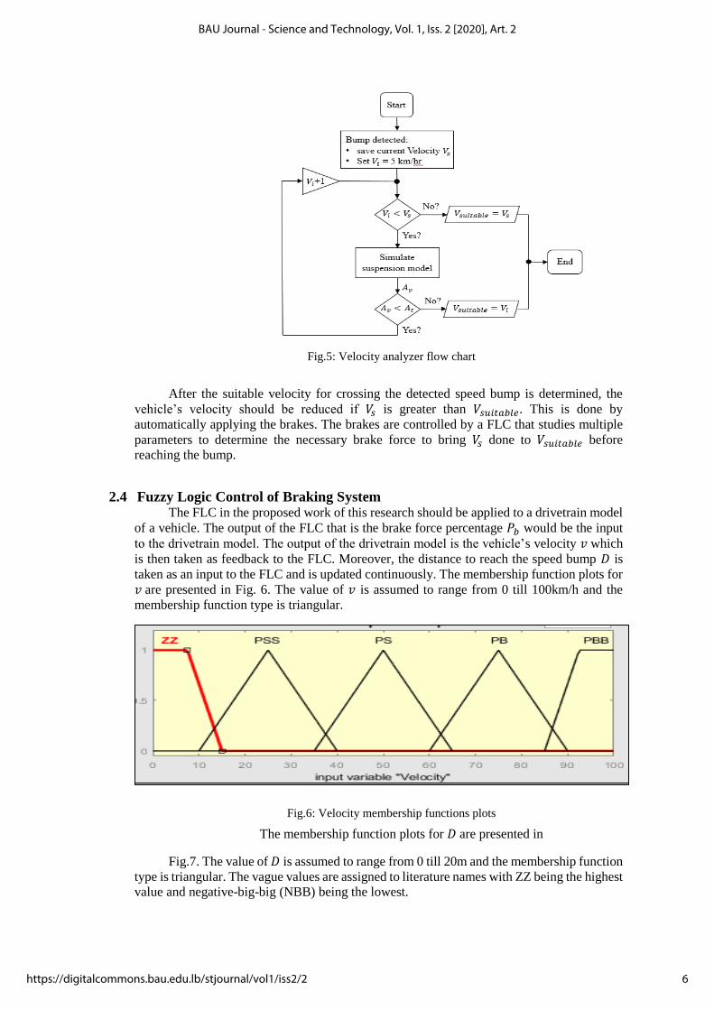
Fig.5: Velocity analyzer flow chart

After the suitable velocity for crossing the detected speed bump is determined, the

vehicle’s velocity should be reduced if 𝑉𝑠 is greater than 𝑉𝑠𝑢𝑖𝑡𝑎𝑏𝑙𝑒. This is done by

automatically applying the brakes. The brakes are controlled by a FLC that studies multiple

parameters to determine the necessary brake force to bring 𝑉𝑠 done to 𝑉𝑠𝑢𝑖𝑡𝑎𝑏𝑙𝑒 before

reaching the bump.

2.4 Fuzzy Logic Control of Braking System The FLC in the proposed work of this research should be applied to a drivetrain model

of a vehicle. The output of the FLC that is the brake force percentage 𝑃𝑏 would be the input

to the drivetrain model. The output of the drivetrain model is the vehicle’s velocity 𝑣 which

is then taken as feedback to the FLC. Moreover, the distance to reach the speed bump 𝐷 is

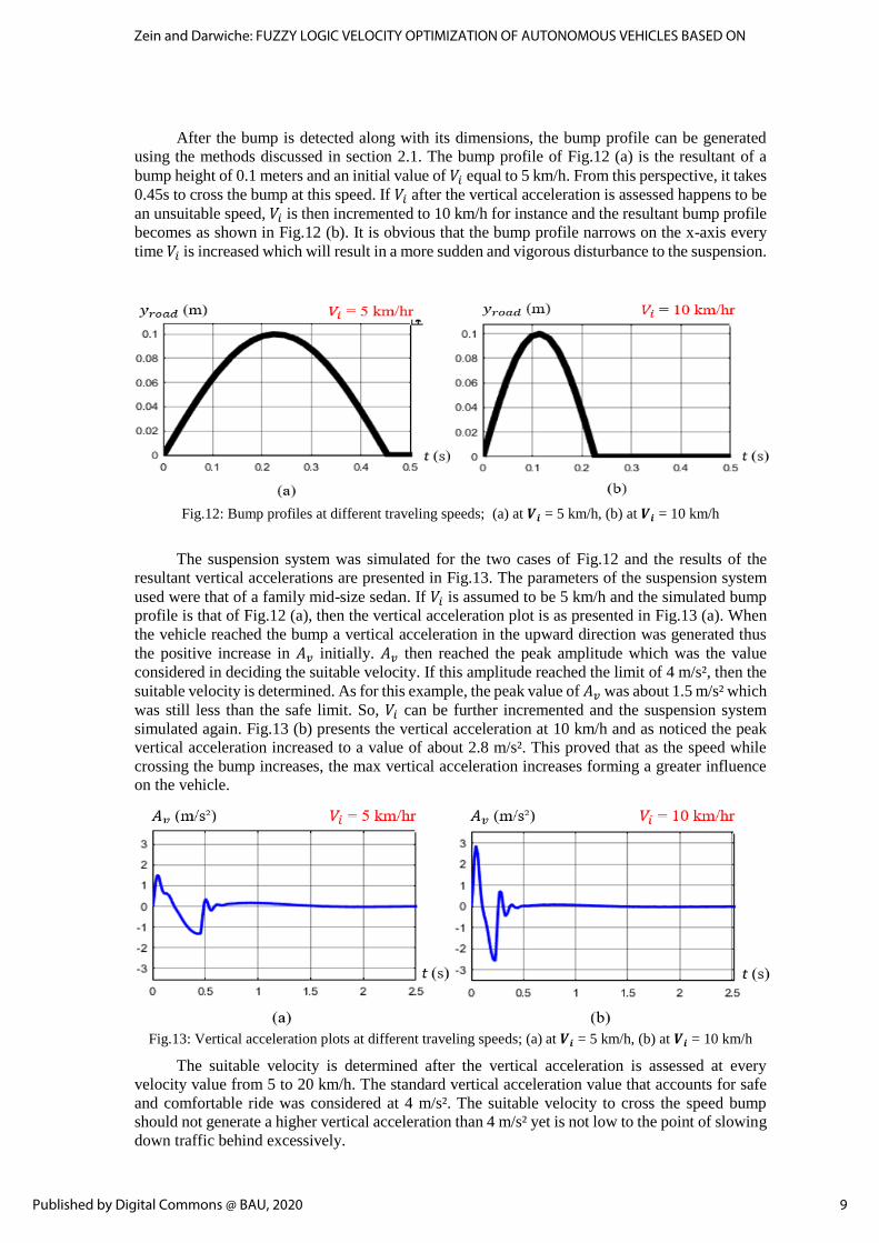
taken as an input to the FLC and is updated continuously. The membership function plots for

𝑣 are presented in Fig. 6. The value of 𝑣 is assumed to range from 0 till 100km/h and the

membership function type is triangular.

Fig.6: Velocity membership functions plots

The membership function plots for 𝐷 are presented in

Fig.7. The value of 𝐷 is assumed to range from 0 till 20m and the membership function

type is triangular. The vague values are assigned to literature names with ZZ being the highest

value and negative-big-big (NBB) being the lowest.

6

BAU Journal - Science and Technology, Vol. 1, Iss. 2 [2020], Art. 2

https://digitalcommons.bau.edu.lb/stjournal/vol1/iss2/2

Fig.7: Distance membership functions plots

The membership function plots for 𝑃𝑏 are presented in

Fig.7. The value of 𝑃𝑏 is assumed to range from 0 till 100% and the membership

function type is triangular. The vague values are assigned to literature names with ZZ being

the lowest value and positive-big-big-big (PBBB) being the highest. By increasing the

number of membership functions for 𝑃𝑏, a more precise response was achieved from the FLC.

Fig.8 Brake percentage membership functions plots

After the fuzzification process, the fuzzy rules were assigned according to Table 1. The

top row of the table includes the linguistic values of 𝒗 while the first column includes that of

𝑫. The middle values are assigned values of the output 𝑷𝒃. These values were tweaked until

the braking response during the simulation of the system was as desired.

Table 1: Fuzzy inference rules

D \ v ZZ PSS PS PB PBB

ZZ ZZ PS PBB PBBB PBBB

NSS ZZ PS PB PBB PBBB

NS ZZ PS PS PB PBB

NB ZZ PSS PS PB PB

NBB ZZ PSSS PSS PS PS

2.5 Drivetrain Model

In order to calculate the necessary brake percentage to reduce the traveling speed to

the suitable one before reaching the speed bump, the FLC braking system is applied to a full

drivetrain model. The full car drivetrain simulation in Matlab, includes all the basic methods

of driveline modeling and many key Simscape™ Driveline™ features (MathWorks, 2019).

The block diagram of Fig 9 presents how the model works. The throttle percentage is the

input to the engine unit which in turn outputs the torque figure to the gearbox unit.

7

Zein and Darwiche: FUZZY LOGIC VELOCITY OPTIMIZATION OF AUTONOMOUS VEHICLES BASED ON

Published by Digital Commons @ BAU, 2020

The gearbox unit includes blocks of the torque converter, gear set, and the automatic

transmission control unit. Its output, the rotational speed, is taken by the vehicle dynamics

block that represents the vehicle’s aerodynamics, mass, dimensions, and brake models. This

block also takes as a disturbance the brake percentage if available.

The output of this block is the vehicle’s traveling speed which is then used as feedback

to the FLC. The joint Simulink model of the FLC braking system and the drivetrain is

presented in Fig.10.

Fig 9: Drivetrain model diagram (MathWorks, 2019)

Fig.10: FLC and drivetrain simulation

3. Results and Discussion In order to validate the proposed methods for the studied system, a simulation using Matlab

and Simulink was conducted. Being a system that combined mechanical design and control

methods, the mentioned programs provide an easy tool to simulate the design, plot results, generate

fuzzy control models, and combine the several sub-systems together. The results to be studied are

presented in Fig. 11 in bold and red text and generated from the correspondent sub-system placed

in a rectangle.

Fig.11: The studied results from the system simulation

8

BAU Journal - Science and Technology, Vol. 1, Iss. 2 [2020], Art. 2

https://digitalcommons.bau.edu.lb/stjournal/vol1/iss2/2

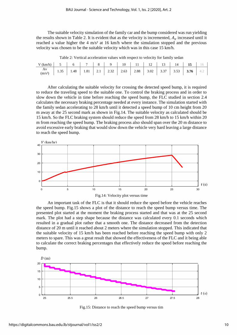
After the bump is detected along with its dimensions, the bump profile can be generated

using the methods discussed in section 2.1. The bump profile of Fig.12 (a) is the resultant of a

bump height of 0.1 meters and an initial value of 𝑉𝑖 equal to 5 km/h. From this perspective, it takes

0.45s to cross the bump at this speed. If 𝑉𝑖 after the vertical acceleration is assessed happens to be

an unsuitable speed, 𝑉𝑖 is then incremented to 10 km/h for instance and the resultant bump profile

becomes as shown in Fig.12 (b). It is obvious that the bump profile narrows on the x-axis every

time 𝑉𝑖 is increased which will result in a more sudden and vigorous disturbance to the suspension.

Fig.12: Bump profiles at different traveling speeds; (a) at 𝑽𝒊 = 5 km/h, (b) at 𝑽𝒊 = 10 km/h

The suspension system was simulated for the two cases of Fig.12 and the results of the

resultant vertical accelerations are presented in Fig.13. The parameters of the suspension system

used were that of a family mid-size sedan. If 𝑉𝑖 is assumed to be 5 km/h and the simulated bump

profile is that of Fig.12 (a), then the vertical acceleration plot is as presented in Fig.13 (a). When

the vehicle reached the bump a vertical acceleration in the upward direction was generated thus

the positive increase in 𝐴𝑣 initially. 𝐴𝑣 then reached the peak amplitude which was the value

considered in deciding the suitable velocity. If this amplitude reached the limit of 4 m/s², then the

suitable velocity is determined. As for this example, the peak value of 𝐴𝑣 was about 1.5 m/s² which

was still less than the safe limit. So, 𝑉𝑖 can be further incremented and the suspension system

simulated again. Fig.13 (b) presents the vertical acceleration at 10 km/h and as noticed the peak

vertical acceleration increased to a value of about 2.8 m/s². This proved that as the speed while

crossing the bump increases, the max vertical acceleration increases forming a greater influence

on the vehicle.

Fig.13: Vertical acceleration plots at different traveling speeds; (a) at 𝑽𝒊 = 5 km/h, (b) at 𝑽𝒊 = 10 km/h

The suitable velocity is determined after the vertical acceleration is assessed at every

velocity value from 5 to 20 km/h. The standard vertical acceleration value that accounts for safe

and comfortable ride was considered at 4 m/s². The suitable velocity to cross the speed bump

should not generate a higher vertical acceleration than 4 m/s² yet is not low to the point of slowing

down traffic behind excessively.

9

Zein and Darwiche: FUZZY LOGIC VELOCITY OPTIMIZATION OF AUTONOMOUS VEHICLES BASED ON

Published by Digital Commons @ BAU, 2020

The suitable velocity simulation of the family car and the bump considered was run yielding

the results shown in Table 2. It is evident that as the velocity is incremented, 𝐴𝑣 increased until it

reached a value higher the 4 m/s² at 16 km/h where the simulation stopped and the previous

velocity was chosen to be the suitable velocity which was in this case 15 km/h.

Table 2: Vertical acceleration values with respect to velocity for family sedan

V (km/h) 5 6 7 8 9 10 11 12 13 14 15 16

Av

(m/s²) 1.35 1.48 1.81 2.1 2.32 2.63 2.88 3.02 3.37 3.53 3.76 4.2

After calculating the suitable velocity for crossing the detected speed bump, it is required

to reduce the traveling speed to the suitable one. To control the braking process and in order to

slow down the vehicle in time before reaching the speed bump, the FLC studied in section 2.4

calculates the necessary braking percentage needed at every instance. The simulation started with

the family sedan accelerating to 28 km/h until it detected a speed bump of 10 cm height from 20

m away at the 25 second mark as shown in Fig.14. The suitable velocity as calculated should be

15 km/h. So the FLC braking system should reduce the speed from 28 km/h to 15 km/h within 20

m from reaching the speed bump. The braking process also should span over the 20 m distance to

avoid excessive early braking that would slow down the vehicle very hard leaving a large distance

to reach the speed bump.

Fig.14: Velocity plot versus time

An important task of the FLC is that it should reduce the speed before the vehicle reaches

the speed bump. Fig.15 shows a plot of the distance to reach the speed bump versus time. The

presented plot started at the moment the braking process started and that was at the 25 second

mark. The plot had a step shape because the distance was calculated every 0.1 seconds which

resulted in a gradual plot rather that a smooth one. The distance decreased from the detection

distance of 20 m until it reached about 2 meters where the simulation stopped. This indicated that

the suitable velocity of 15 km/h has been reached before reaching the speed bump with only 2

meters to spare. This was a great result that showed the effectiveness of the FLC and it being able

to calculate the correct braking percentages that effectively reduce the speed before reaching the

bump.

Fig.15: Distance to reach the speed bump versus tim

10

BAU Journal - Science and Technology, Vol. 1, Iss. 2 [2020], Art. 2

https://digitalcommons.bau.edu.lb/stjournal/vol1/iss2/2

Fig.16 shows how the braking percentage changed during the braking process. The

percentage was zero while the vehicle was accelerating until the 25 second mark was reached. The

braking process started at 20% braking and increased gradually until reaching 50% by the end of

the process. This showed that the brakes were lightly applied at first so that drivers behind will

not be surprised by a sudden braking of the vehicle in front of them. As the vehicle approached

the bump more and more, the percentage increased until the simulation ended where the suitable

velocity has been reached.

Fig.16: Brake percentage versus time

4. CONCLUSIONS A- With car safety features rapidly developing in the past decade, few car manufacturers

developed systems that account for road conditions where most of these systems had to do

with coping the suspension system to different terrains but not for potholes or speed bumps.

B- Several vehicles today have autopilot systems that virtually require no input from the driver

in certain situations with such systems getting more and more advanced but the road

conditions and infrastructure of most countries have not changed.

C- Until the time comes where all vehicles are autonomous and the road infrastructure is entirely

updated, autopilot systems should account for speed bumps since crossing the speed bump at

a high speed may lead to serious consequences.

D- This research presented a full system that can aid the autopilot in reducing the

vehicle’s speed if it encountered a speed bump by detecting it before the vehicle

reaches it and then assessing its dimensions to calculate the resulting vertical

accelerations to determine the suitable speed that provides the optimal bump crossing.

E- After that the FLC braking system calculates the necessary brake percentage to reduce

the vehicle’s speed before reaching the speed bump providing a safe and controlled

deceleration of the vehicle.

F- The system studied in this research can be improved to detect speed bumps of several

shapes and also potholes and other road irregularities and also improving the

suspension model from a quarter car model to a full model that assesses the vertical

accelerations at the passengers instead of the top of the wheels.

ACKNOWLEDGEMENT I must first acknowledge my thesis supervisor Dr. Mohamad Darwiche for all the guidance and

knowledge he provided that yielded this work. I can only express sincere gratitude and thankfulness

to him for aiding me in completing this quest. I would like to thank all the mechanical engineering

teaching staff for choosing me for the fully paid master scholarship ahead of them the head of the

Mechanical Engineering department Prof. Ali Hammoud. All of what I accomplished till now could

not be possible without the aid provided by my parents. A big appreciation goes to them for their

patience and sacrifices they made to get me into a prestigious university like BAU.

REFERENCES

- Aleksendrić, D., Jakovljević, Ž., & Ćirović, V. (2012). Intelligent control of braking process.

Expert Systems with Applications, 39(14), 11758-11765.

11

Zein and Darwiche: FUZZY LOGIC VELOCITY OPTIMIZATION OF AUTONOMOUS VEHICLES BASED ON

Published by Digital Commons @ BAU, 2020

- Devapriya, W., Babu, C. N., & Srihari, T. (2016). Real Time Speed Bump Detection Using

Gaussian Filtering and Connected Component Approach. Scientific Research Publishing, 2168-

2175.

- Eriksson, J., Girod, L., Hull, B., Newton, R., Madden, S., & Balakrishnan, H. (2008). The Pothole

Patrol: Using a Mobile Sensor Network for Road Surface Monitoring. 6th Annual International

Conference on Mobile Systems, Applications and Services (MobiSys). Breckenridge.

- Gordon, M. (2013, October 31). Strava Support. Retrieved february 22, 2018, from

www.support.strava.com

- HowStuffWorks.com. (1, April 2000). Retrieved August 23, 2018, from

www.auto.howstuffworks.com

- Janczur, R. (2012). Vertical Accelerations Of The Body Of A Motor Vehicle When Crossing A

Speed Bump. Cracow: Cracow University of Technology.

- Kanjanavapastit, A., & Thitinaruemit, A. (2012). Estimation of a Speed Hump Profile Using

Quarter Car Model. International Science, Social Science, Engineering and Energy Conference.

Thailand.

- Lin, C., Chen, J., Su, P., & Chen, C. (2014). Eigen-feature Analysis of Weighted Covariance

Matrices for LIDAR Point Cloud Classification. ISPRS, 70-79.

- Madli, R., Hebbar, S., Pattar, P., & Golla, V. (2015). Automatic Detection and Notification of

Potholes and Humps on Roads to Aid Drivers. IEEE Sensors Journal, 15(8), 4313 - 4318.

- MathWorks .(2019). Complete Vehicle Model. Retrieved August 25, 2019, from

www.mathworks.com

- MathWorks .(2019). Modeling an Automatic Transmission Controller. Retrieved August 25,

2019, from www.mathworks.com

- Milanés, V., Shladover, S. E., Spring, J., Nowakowski, C., Kawazoe, H., & Nakamura, M. (2014).

Cooperative Adaptive Cruise Control in Real Traffic Situations. IEEE Transactions on Intelligent

Transportation Systems, 15(1), 296 - 305.

- Miyata, S., Nakagami, T., Kobayashi, S., Izumi, T., Naito, H., Yanou, A., . . . Takehara, S. (2010).

Improvement of Adaptive Cruise Control Performance. EURASIP Journal on Advances in Signal

Processing, 3(5), 50-64.

- Moon, S., Yi, K., & Kang, H. (2008). Multi-Vehicle Adaptive Cruise Control with Collision.

AVEC. Seoul, Korea.

- Pan, Z., Bao, H., Pan, F., & Xu, C. (2016). An Intelligent Vehicle Based on an Improved PID

Speed Control Algorithm for Driving Trend Graphs. International Journal of Simulation --

Systems, Science & Technology, 17(30), 19.1-19.7.

- Redmon, J., Divvala, S., Girshick, R., & Farhadi, A. (2016). You Only Look Once: Unified, Real-

Time Object Detection. IEEE Conference on Computer Vision and Pattern Recognition. Las

Vegas.

- Ramesh, S., Ranjan, R., Mukherjee, R., & Chaudhuri, S. (2012). Vehicle Collision Avoidance

System Using Wireless Sensor Networks”. International Journal of Soft Computing and

Engineering (IJSCE), 2(5).

- Sabatini, R., Gardi, A., & Richardson, M. A. (2014). LIDAR Obstacle Warning and Avoidance

System for Unmanned Aircraft. International Journal of Mechanical, Aerospace, Industrial and

Mechatronics Engineering, 8, 704-715.

- Sharma, B. (2019, 1 30). What is LiDAR technology and how does it work? Geospatial World.

- Szegedy, C., Reed, S., Erhan, D., Anguelov, D., & Ioffe, S. (2014). Scalable, High-quality Object

Detection. arXiv, 1412-1441.

- Trebli-Olennu, A., Dolan, J. M., & Khosla, P. K. (2001). Adaptive fuzzy throttle control for an

all-terrain vehicle. Journal of Systems and Control Engineering, 16(3), 121-132.

- Wei, P., Ball, J., & Anderson, D. (2018). Fusion of an Ensemble of Augmented Image Detectors

for Robust Object Detection. Sensors, 894.

- Wen, W. (2008). Road Roughness Detection by. Stockholm, Sweden: School of Architecture and

the Built Environment.

12

BAU Journal - Science and Technology, Vol. 1, Iss. 2 [2020], Art. 2

https://digitalcommons.bau.edu.lb/stjournal/vol1/iss2/2