Embed Size (px)
Citation preview
A Fuzzy Controller
for Three Dimensional Line Following of an
Unmanned Autonomous Mobile Robot
A thesis submitted to the
Division of Research and Advanced Studiesof the University of Cincinnati
in partial fulfillment of therequirements for the degree of
MASTER OF SCIENCE
in the Department of Mechanical, Industrial, and Nuclear Engineeringof the College of Engineering
1997
by
Nikhil D KelkarB. S from Government College of Engineering Pune (India)
Committee Chair : Dr. Ernest Hall
ii
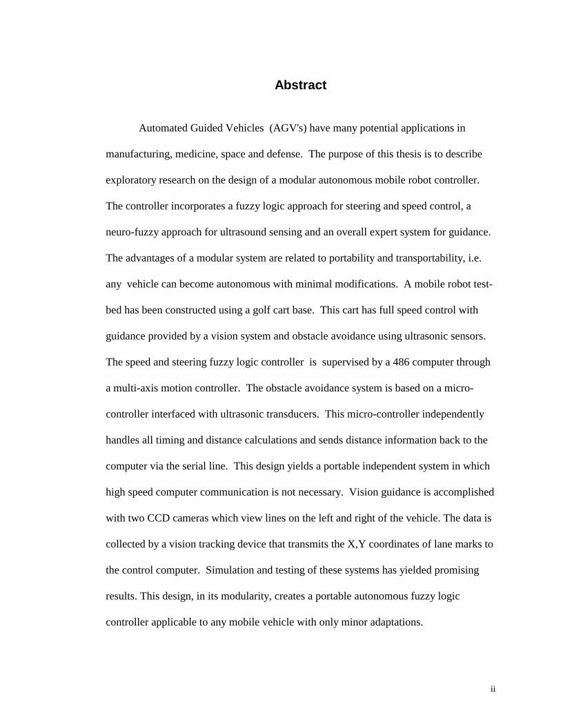
Abstract
Automated Guided Vehicles (AGV's) have many potential applications in
manufacturing, medicine, space and defense. The purpose of this thesis is to describe
exploratory research on the design of a modular autonomous mobile robot controller.
The controller incorporates a fuzzy logic approach for steering and speed control, a
neuro-fuzzy approach for ultrasound sensing and an overall expert system for guidance.
The advantages of a modular system are related to portability and transportability, i.e.
any vehicle can become autonomous with minimal modifications. A mobile robot test-
bed has been constructed using a golf cart base. This cart has full speed control with
guidance provided by a vision system and obstacle avoidance using ultrasonic sensors.
The speed and steering fuzzy logic controller is supervised by a 486 computer through
a multi-axis motion controller. The obstacle avoidance system is based on a micro-
controller interfaced with ultrasonic transducers. This micro-controller independently
handles all timing and distance calculations and sends distance information back to the
computer via the serial line. This design yields a portable independent system in which
high speed computer communication is not necessary. Vision guidance is accomplished
with two CCD cameras which view lines on the left and right of the vehicle. The data is
collected by a vision tracking device that transmits the X,Y coordinates of lane marks to
the control computer. Simulation and testing of these systems has yielded promising
results. This design, in its modularity, creates a portable autonomous fuzzy logic
controller applicable to any mobile vehicle with only minor adaptations.

iii
Acknowledgment
First and foremost, I wish to express my deep gratitude to my dissertation
advisor, Paul E. Geier Professor of Robotics, Dr. Ernest Hall, for all his valuable
guidance, assistance and support throughout my graduate studies at the University of
Cincinnati. It was Dr. Hall who introduced me to this field and helped me to understand
this technology.
I wish to thank the members of my master's defense committee for their
suggestions and support on this research. Their comments on this research are greatly
appreciated.
I also gratefully acknowledge the assistance and support of all the graduate and
undergraduate students of the Center for Robotics Research. I would like to thank
Tayib Samu for his support in this research.
My parents have encouraged me throughout my education and career, and I will
always be grateful for their sacrifice, generosity and love.
Most importantly I extend my gratitude to my wife Dipti for her support,
patience and assurance during my pursuit for higher studies.
iv
Table of Contents
ABSTRACT...................................................................................................................... II
ACKNOWLEDGMENT ................................................................................................ III
CHAPTER 1. INTRODUCTION....................................................................................1
1.1 OBJECTIVE......................................................................................................................2
1.2 FUZZY LOGIC..................................................................................................................3
1.2.1 History, Research & Applications ...........................................................................3
1.3 OUTLINE OF THE THESIS..................................................................................................7
CHAPTER 2. THEORY OF FUZZY SETS...................................................................8
2.1 BASIC CONCEPTS...........................................................................................................10
2.2 DEFINITIONS .................................................................................................................10
2.2.1 Definition 1...........................................................................................................10
2.2.2 Definition 2...........................................................................................................10
2.2.3 Definition 3...........................................................................................................10
2.2.4 Definition 4...........................................................................................................11
2.3 OPERATIONS ON FUZZY SETS.........................................................................................12
2.3.1 Fuzzy complement..................................................................................................12
2.3.2 Fuzzy union............................................................................................................14
2.3.3 Fuzzy intersection..................................................................................................16
2.3.4 Aggregation operator ............................................................................................18
2.4 FUZZY LOGIC (FL) ........................................................................................................19
v
2.4.1 Fuzzy implication operators ..................................................................................20
CHAPTER 3. FUZZY LOGIC CONTROLLER.........................................................21
3.1 FUZZY INFERENCE SYSTEM...........................................................................................21
3.2 FUZZY SET DEFINITION .................................................................................................22
3.2.1 Input fuzzy sets.......................................................................................................23
3.2.2 Output fuzzy set......................................................................................................24
3.3 FUZZIFICATION..............................................................................................................26
3.4 RULE BASE...................................................................................................................26
3.5 FUZZY OPERATORS.......................................................................................................29
3.6 IMPLICATION .................................................................................................................30
3.7 AGGREGATION..............................................................................................................31
3.8 DEFUZZIFICATION .........................................................................................................31
CHAPTER 4. ABOUT THE COMPETITION AND AGV DESIGN........................36
4.1 OBJECTIVE....................................................................................................................37
4.2 ENVIRONMENT..............................................................................................................37
CHAPTER 5. CONTROL..............................................................................................38
5.1 VISION GUIDANCE AND DATA INPUT..............................................................................38
5.2 OBSTACLE AVOIDANCE ................................................................................................41
5.2.1 Pseudo code for obstacle avoidance .....................................................................42
CHAPTER 6. RESULTS................................................................................................45
6.1 MATLAB SIMULATIONS .................................................................................................47
vi
6.1.1 Case 1: Straight Line.............................................................................................47
6.1.2 Case 2: Curved Path .............................................................................................49
6.1.3 Case 3: Sensitivity to distance variation ...............................................................50
6.1.4 Case 4: Sensitivity to angular fluctuations............................................................51
6.1.5 Case 5: Extreme environment................................................................................52
CHAPTER 7. CONCLUSION AND RECOMMENDATIONS .................................54
7.1 CONCLUSION.................................................................................................................54
7.2 FUTURE RECOMMENDATIONS.......................................................................................56
REFERENCES.................................................................................................................58
APPENDIX.......................................................................................................................63
A. FLOW CHART FOR THE CONTROL ALGORITHM................................................................63
B. FUZZY LOGIC CONTROLLER: C PROGRAM.......................................................................64
Header Files:..................................................................................................................64
Main control code...........................................................................................................66
Fuzzy Controller.............................................................................................................72
Fuzzification algorithm used by the fuzzy controller .....................................................79
Vector and Point Operations..........................................................................................81
C. STEERING ANGLE OUTPUT TABLE FOR DIFFERENT DISTANCE AND ANGLE INPUTS. ...........85
D. FUZZY ASSOCIATED MEMORIES.....................................................................................86
E. MATLAB SIMULATION DATA ...........................................................................................87
Case 1:............................................................................................................................87
Case 2:............................................................................................................................87

vii
Case 3:............................................................................................................................88
Case 4:............................................................................................................................89
Case 5:............................................................................................................................90

viii
List of Tables
Table 1. Input fuzzy sets__________________________________________________23
Table 2. Input fuzzy sets__________________________________________________24
Table 3. Output fuzzy sets ________________________________________________25
Table 4. Results of simulation______________________________________________46
ix
List of Figures
Figure 1. Schematic of the control strategy___________________________________21
Figure 2. Input membership functions for angle error __________________________23
Figure 3. Input membership functions for distance error ________________________24
Figure 4. Output membership functions for steering angle correction ______________25
Figure 5. Illustration of fuzzy implication and the center of gravity defuzzification____32
Figure 6. Rule base _____________________________________________________33
Figure 7. Rule surface for the Fuzzy Controller _______________________________34
Figure 8. UC Robot Club robot “BEARCAT” ________________________________36
Figure 9. Schematic of the robot running in its environment _____________________37
Figure 10. Path correction _______________________________________________41
Figure 11. Obstacle avoidance ____________________________________________52
Figure 12. Results: Case______________________________________________56
Figure 13. Results: Case 2______________________________________________57
Figure 14. Results: Case 3______________________________________________58
Figure 15. Results: Case 4______________________________________________59
Figure 16. Results: Case 5______________________________________________60
1
Chapter 1. Introduction
Controller design for any system needs some knowledge about the system.
Usually this involves a mathematical description of the relation among inputs to the
process, its state variables, and its output. This description is called the model of the
system. The model can be represented as a set of transfer functions for time invariant
linear systems or other relationships for non-linear or variant systems.
Modeling complex systems can be a very difficult task. In a complex system such
as a multiple input and multiple output system, inaccurate models can lead to unstable
systems, or unsuitable system performance. Fuzzy Logic Control (FLC) is an effective
alternative approach for systems which are difficult to model. The FLC uses the
qualitative aspects of the human decision process to construct the control algorithm. This
can lead to a robust controller design. The modeling of a mobile robot is a very complex
task and a direct application of FLC can be found in this area.
An excellent introduction to the mathematical analysis of mobile robots can be
found in a study by Muik and Neuman 1. Even though the visualization and recognition of
image information for the guidance of mobile robot have been studied for years, 2-7 the
design of a mobile system is a challenging task. The challenge of designing an intelligent
controller is in determining what information to measure and how to use this information
in a manner that will satisfy the performance specifications of the machine. Several fuzzy
logic approaches for modeling control systems for vehicles have been studied in the past.
A fuzzy logic controller 8 that guarantees stability of a control system for a computer-
2
simulated model car and advanced fuzzy logic application for automobiles application
was discussed in Altrock et. al. 9.
Objective
The main aspect of intelligent control addressed in this thesis is the design of a
controller for a mobile robot using fuzzy logic. The design specifications were to build a
robot which could follow a line, avoid obstacles, and adapt to variations in terrain. The
adaptive capabilities of a mobile robot depend on the fundamental analytical and
architectural designs of the sensor systems used. The mobile robot provides an excellent
test bed for investigations into generic vision guided robot control since it is similar to an
automobile and is a multi-input, multi-output system. An algorithm was developed to
establish a mathematical and geometrical relationship between the physical three
dimensional (3-D) ground coordinates of the line to follow and its corresponding two
dimensional (2-D) digitized image coordinates. This relationship is incorporated into the
vision tracking system to determine the perpendicular distance and angle of the line with
respect to the centroid of the robot. The information from the vision tracking system was
used as input to a closed loop fuzzy logic controller to control the steering and the speed of
the robot.
3
Fuzzy Logic
History, Research & Applications
Fuzzy logic was first proposed by Lotfi A. Zadeh of the University of California
at Berkeley in a 1965 paper; he elaborated on his ideas in a 1973 paper 10 that
introduced the concept of "linguistic variables". In his approach, a fuzzy implication is
defined as a fuzzy cartesian product. Based on Zadeh's definition of implication,
Mamdani 11 built the first fuzzy logic controller.
Other implications have been studied by Baldwin and Guild 12 and Baldwin and
Pilsworth 13. They have proposed the following properties of implication: fundamental
property, smoothness property, unrestricted inferences, modus ponens, modus tollens
symmetry, and propagation of fuzziness.
Research concerning applicability of various implications in fuzzy model has
been conducted by Kiszka 14 and then by Cao and Kandel 15. Using linguistic
descriptions of a d.c series motor, Kiszka constructed its fuzzy model using 36 fuzzy
implications and two different interpretations of connective ALSO. He developed a
root-mean-square error, as well as the number of mathematical operations, required to
obtain the fuzzy model, such as a criterion of applicability given a fuzzy implication.
Cao extended the investigation to different physical systems, with different fuzzy sets
used to interpret the linguistic terms.
In 1995 Maytag introduced an "intelligent" dishwasher based on a fuzzy
controller and a "one-stop sensing module" that combines a thermistor (for temperature
4
measurement), a conductivity sensor (to measure detergent level from the ions present
in the wash), a turbidity sensor that measures scattered and transmitted light to measure
the soiling of the wash, and a magnetostrictive sensor to read spin rate. The system
determines the optimum wash cycle for any load to obtain the best results with the least
amount of energy, detergent, and water; it even adjusts for dried-on foods by tracking
the last time the door was opened and estimates the number of dishes by the number of
times the door was opened.
For the last 20 years, Fuzzy Control Theory has emerged as a fruitful approach
to a wide variety of control problems 16,17,18,19,20,21,22,24.
During an international meeting of fuzzy logic researchers in Tokyo, Takeshi
Yamakawa 24 demonstrated the use of fuzzy control (through a set of simple dedicated
fuzzy logic chips) in an "inverted pendulum" experiment -- a classic control problem in
which a vehicle tries to keep a pole (mounted on its top) by a hinge upright by moving
back and forth. Observers were impressed with this demonstration, as well as later
experiments by Yamakawa in which he mounted a wine glass containing water or even
a live mouse to the top of the pendulum; the system maintained stability in both cases.
Yamakawa eventually went on to organize his own fuzzy-systems research lab to help
develop his patents in the field.
A comparison of Fuzzy Logic, Proportional Integrated Derivative (PID) and
Sliding Mode Control is presented by Coleman and Godbole 25. They conclude that
Fuzzy Logic is a very robust control tool for a control engineer. In their paper 25 they
present a comparison of Fuzzy Logic Control and Classical Control Design
5
methodologies. The Fuzzy Logic Control achieved all the goals that the PID and sliding
mode control is normally used to achieve.
Zhou, McLauchlan, Challoo and Omar 26 have presented a Fuzzy Logic Control
of a four-link robotic manipulator in a vertical plane. A non-algorithmic, model free
approach has been developed that relies on a fuzzy rule base to evaluate the required
axis motion to result in the desired two-dimensional end point motion. This scheme
does not require solution of complex nonlinear inverse kinematics equations to arrive at
the joint control commands. This is in contrast with the traditional robot controllers.
The fuzzy rule base control provided a fast execution speed.
Research and development is also continuing on fuzzy applications in software
(as opposed to firmware) design, including fuzzy expert systems and integration of
fuzzy logic with neural-network and evolutionary adaptive "genetic" software systems,
with the ultimate goal of building "self-learning" fuzzy control systems; however, this
subject is beyond the scope of this thesis.
Research Objective
The main goal of this research is to model a modular Fuzzy Logic Control for an
automated guided vehicle and test the performance of the vehicle in a real time
environment. The research is focused on the design of the Fuzzy Controller for vision
and sonar navigation of the automated guided vehicle.
6
The design of the controller was done in three stages.
In the first stage the universe of discourse was identified and fuzzy sets are
defined. The rule base (Fuzzy Control Rules) for the control was defined through a
human decision making process. The membership functions and their intervals are
defined. Aggregation and defuzzification methods are selected.
In the second stage the Fuzzy Controller was coded in C programming language
and implemented on the autonomous guided vehicle. Then the performance of the
controller was then tested through a series of simulations and real time running of the
vehicle.
In the third and final stage, the rule base and the membership functions were
tuned to improve the performance of the vehicle.

7
Outline of the thesis
The fundamentals of the fuzzy set theory and fuzzy logic theory are presented in
Chapter 2. The discussion includes basic definitions and concepts used in this research.
Chapter 3 contains a detailed description on the Fuzzy Logic Controller. The
algorithm used in the research is described in detail. The concept of Binary Fuzzy
Associative Memory is presented.
Chapter 4 has a brief introduction to the Autonomous Guided Vehicle Project
"Bearcat" and the international Ground Robotics Competition.
Chapter 5 deals with data input for vision navigation and the details of the fuzzy
sets, rule base, membership functions and implication operators.
Chapter 6 presents the results of simulation runs using MATLAB with detail a
detail review of a few selected cases. It also contains a small summary of the real time
testing on the robot.
Finally the conclusions for this research are presented in Chapter 7. The
simulation programs and the source code for the fuzzy controller are listed in the
appendices.
8
Chapter 2. Theory of Fuzzy Sets
Fuzzy set and fuzzy logic theories are reviewed in this chapter. These theories
are the basis of fuzzy logic control. The definitions and concepts presented in this
chapter are based on Novak and Klir 28 and Folger 28. The information is repeated in
this chapter for completeness and to introduce and clarify the notation used in the rest of
this thesis.
The fuzzy set is essentially a generalization of the classical or ordinary set. The
ordinary set is defined in such a way that individuals in some given universe of
discourse are divided into two groups: members - those that certainly belong in the set
and non-members - those that certainly do not. A sharp unambiguous distinction exists
between the members and non-members of the class or category represented by the
ordinary set. Many of the categories commonly employed to describe our perception of
reality do not exhibit this sharp distinction. For example, there is no sharp distinction
between the classes of luxury cars, moderately expensive cars and economy cars.
Instead, their boundaries are vague, and the transition from member to non-member is
gradual rather than abrupt. Thus, the fuzzy set introduces vagueness by eliminating the
sharp boundaries dividing members of the class from non-members. Mathematically, a
fuzzy set is defined by assigning to each individual in the universe of discourse a value
in the interval [0, 1] representing its grade of membership in the fuzzy set. This grade
corresponds to the degree to which that individual is similar to or compatible with the
concept represented by the fuzzy set. Thus, individuals may belong in a fuzzy set to a

9
greater or lesser degree indicated by a larger or smaller membership grade. Full
membership and full non-membership are indicated by membership grade of 1 and 0,
respectively.
10
Basic concepts
Definitions
Definition 1
Let C be an ordinary set called the universe of discourse that may be either
discrete or continuous and let U be the function taking values from the interval [0,1 ].
The fuzzy subset C in the universe of discourse C maybe represented by the function:
U C: [ , ]� �� 01 (1)
where U is called the membership function of fuzzy set C:
Thus the fuzzy subset C in C is represented as a set of ordered pairs of an
element c and its membership function:
C U c c c C� � �{( ( ) / )| } (2)
When a membership function takes only the values 1 or 0, the fuzzy set becomes
the ordinary set. The value of the membership function for a given element of a fuzzy
set is called the membership grade.
Definition 2
The support of fuzzy set C is an ordinary set defined as:
su C c U c( ) { : ( ) }� � 0 (3)
Definition 3
The � -cut of the fuzzy set C for the given � is an ordinary set:
11
C c U c( ) { : ( ) }� �� � (4)
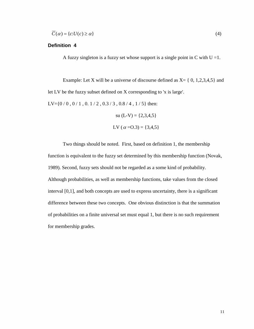
Definition 4
A fuzzy singleton is a fuzzy set whose support is a single point in C with U =1.
Example: Let X will be a universe of discourse defined as X= { 0, 1,2,3,4,5} and
let LV be the fuzzy subset defined on X corresponding to 'x is large'.
LV={0 / 0 , 0 / 1 , 0. 1 / 2 , 0.3 / 3 , 0.8 / 4 , 1 / 5} then:
su (L-V) = {2,3,4,5}
LV (� =O.3) = {3,4,5}
Two things should be noted. First, based on definition 1, the membership
function is equivalent to the fuzzy set determined by this membership function (Novak,
1989). Second, fuzzy sets should not be regarded as a some kind of probability.
Although probabilities, as well as membership functions, take values from the closed
interval [0,1], and both concepts are used to express uncertainty, there is a significant
difference between these two concepts. One obvious distinction is that the summation
of probabilities on a finite universal set must equal 1, but there is no such requirement
for membership grades.
12
Operations on fuzzy sets
The three basic operations on fuzzy sets are: complement, union, and
intersection. The basic operations are defined as functions that satisfy certain axiomatic
requirements and operate on membership grades of fuzzy sets. The results of these
operations are membership functions of new fuzzy sets representing the concept of
fuzzy complement, union, and intersection.
Fuzzy complement
In order for any function com : [0, 1]� [0, 1] to be defined as a fuzzy
complement, the following requirements need to be fulfilled:
Axiom 1 For any fuzzy compliment com (com(0))= 1 and com(l)=0
Axiom 2 For all a, b� [0, 1], if a < b then com(a) > com(b)
In most cases of practical significance, the class of function that can be defined
as fuzzy complement must be narrowed. Thus, two additional axioms are introduced:
Axiom 3 com is a continuous function.
Axiom 4 com is involute, which means that com(com(a)) = a for all a � [ 0, 1].
Axiom 1 assures that fuzzy complement does not violate the complement for
ordinary sets. Moreover an increase in the degree of membership in a fuzzy set should
cause a decrease in the degree of membership of its complement. This is provided by
Axiom 2. Axioms 1 and 2 are called the axiomatic skeleton for fuzzy complement. The
basic complement operator is given below:

13
For example let
LV = {0 / 0 , 0 / 1 , 0. 1 / 2 , 0.3 / 3 , 0.8 / 4 , 1 / 5}
be a fuzzy set then, the fuzzy complement is given as
-LV = {0 / 0 , 1 / 1 , 0. 9 / 2 , 0.7 / 3 , 0.2 / 4 , 0 / 5}
14
Fuzzy union
The fuzzy union is in general a function U of the form u : [0, 1] x [0, 1]� [0,
1]. For each element x in the universal set, this function takes as its argument the pair
consisting of the element's membership grades in set A and in set B and yields the
membership grade of the element in the set constituting the union of A and B. Thus:
U(x) = U� �U U xA B, ( ) (5)
where U(x) is membership function of fuzzy union A � B
This function has to satisfy the following requirements:
Axiom 1 U(0,0) = 0 and U(0,1) = U(1,O) = u(l,l) = 1
Axiom 2 U(a,b) = U(b,a).
Axiom 3 If a � b and c � d, then U(a,c) � U(b,d) (U is monotonic)
Axiom 4 U(U(a,b),c) = U(a,U(b,c)) ( U is associative)
The first axiom ensures that the fuzzy union is a generalization of the classical
union for ordinary sets. This axiom is analogous to the first axiom for fuzzy
compliment. The second axiom indicates indifference to the order in which the sets are
combined in fuzzy union. The third axiom is the natural requirement that a decrease in
the degree of membership in fuzzy sets can not produce an increase in the degree of
membership of their union. Finally, the fourth axiom allows one to extend the fuzzy
union operation for any number of fuzzy sets. As used in the discussion of the fuzzy
complement two additional axioms are formulated. These are:
Axiom 5 U is continuous function.
Axiom 6 U(a,a) = a

15
The axiom of continuity prevents a situation, where a small change in the
membership grade in fuzzy sets produces a large change in the membership grade in
their union. Axiom 6 ensures that the union of any fuzzy set with itself yields precisely
the same set. Based on the above definitions, many union operators can be formulated.
The most important and most used in approximate reasoning are:
Max union a � b = max(a, b)
Algebraic sum a � b = a + b - ab
Bounded sum a � b = min(l,a + b)
Drastic sum a � b= a when b = 0
a � b= b when a = 0
a � b= 0 when a,b � 0
Disjoint sum a � b = max(min(a, 1 - b), min(l - a, b))
16
Fuzzy intersection
The fuzzy intersection is defined as a function i such that 1:
[0, 1] x [0, 1]� [0, 1]. For each element x in the universal set, this function takes as
its argument the pair consisting of the element's membership grades in set i and in set
B,and yields the membership grade of the element in the set constituting the union of A
and B. Thus:
U(x) = i� �U U xA B, ( ) (6)
where U(x) is membership function of fuzzy union A B
This function has to satisfy the following conditions:
Axiom 1 i(0,0) = 0 and i(0, 1) = i(1,0) = i(l, 1) = 1
Axiom 2 i(a,b) = i(b,a).
Axiom 3 If a � b and c � d, then i(a,c) i(b,d) � (U is monotonic)
Axiom 4 i(i(a,b),c) = i(a,i(b,c)) ( i is associative)
Axiom 5 i is continuous function.
Axiom 6 i(a,a) = a
The fulfillment of the two last axioms is unnecessary. The motivation for the
above conditions is the same as for fuzzy union. Moreover, all axioms, except the first,
are identical to axioms formulated for fuzzy union. The first axiom states that fuzzy
intersection has to reduce to ordinary set intersection when the grade of membership is
restricted to 0 and 1. There is an infinite number of functions that can be used as fuzzy
17
intersection, however only a few of them have been employed in approximate
reasoning. These are:
Min Intersection a b = min(a, b)
Algebraic product a b = - ab
Bounded product a b = max(0, a + b - 1)
Drastic product a b= a when b = 1
a b= b when a = 1
a b= 0 when a,b < 1
18
Aggregation operator
Aggregation operations on fuzzy sets are operations by which several fuzzy sets
are combined to produce a single set. In general, any aggregation operation may be
defined by the function
h: [0,1]n � [0,1] (7)
where n is a number of aggregated fuzzy sets
This function has to satisfy the following axiomatic requirements:
Axiom 1 h(0,0,......,0) = 0 and h (1,l,......,1) = 1 ( boundary conditions).
Axiom 2 h is monotonic non-decreasing in all its arguments.
Therefore fuzzy unions and intersections qualify as aggregation operations on
fuzzy sets. They can be viewed as special aggregation operations that are symmetric,
usually continuous, and required to satisfy some additional boundary conditions. The
simplest aggregation operators are:
- -min. intersection - ^
- max. union - V
19
Fuzzy Logic (FL)
The natural consequence of fuzzy set theory is fuzzy logic. The logic
connectives AND and OR are defined based on fuzzy set operations. Fuzzy AND
corresponds to fuzzy intersection operator and fuzzy OR to fuzzy union.
In Boolean logic that is based on ordinary set theory, one can have only two
logic values. Any element can be only in one of two possible relations to the set: it can
belong to the set or not belong. Therefore something can be only true or false. It can be
seen easily that this logic is unrealistic. Usually it is difficult to absolutely state that
something is true of false. More often one simply does not know, or knows
subjectively.
For example the logic value of a statement:
"Jimmy is tall" /and Jimmy is 5'10"/ can not be evaluated by Boolean logic.
Such problems are nonexistent in fuzzy logic. Fuzzy sets introduce intermediate
logic values. Now, logical value can be any number within the interval [0, 1]. Values 0
and 1 mean that something is absolutely false or absolutely true. If the logic value of a
given statement is somewhere between 0 and 1, for example 0.7, it means that this
statement is close to the absolute truth with strength 0.7 or, that this is more true than
false. Therefore, fuzzy logic is more flexible than Boolean logic and closer to reality.
20
Fuzzy implication operators
Fuzzy implication is one of the crucial elements in FLC. These implication
operators interpret the information in linguistic statements and present it in a form to
facilitate decision making by the FL controller. Every control rule of the FL controller
rule base is expressed as a fuzzy relation.
The fuzzy implication is defined as a combination of fuzzy conjunction - fuzzy
logic operator AND, fuzzy disjunction - fuzzy logic OR, and fuzzy negation. These
operators were defined in the previous section in terms of operations on fuzzy sets. The
correspondences among the logic operators and fuzzy set operators are shown below:
FUZZY SET THEORY FUZZY LOGIC
fuzzy intersection i fuzzy conjunction AND
fuzzy union u fuzzy disjunction OR
fuzzy complement com fuzzy negation NOT
Example Implications:
Mamdani implication :a=>b=min(a,b) is just fuzzy conjunction defined by the min
intersection operator.
21
Chapter 3. Fuzzy logic controller
The Fuzzy Logic Controller uses the fuzzy set and fuzzy logic theory previously
introduced in its implementation. A detailed reference on how to design a fuzzy
controller can be found in 29,30,31.
Fuzzy Inference System
Fuzzy inference is the actual process of mapping from a given input to an output
using fuzzy logic 27. Fuzzy logic starts with the concept of a fuzzy set. A fuzzy set is a
set without a crisp, clearly defined boundary. It can contain elements with only a partial
degree of membership. The MATLAB Fuzzy Logic Toolbox was used to build the
initial experimental fuzzy inference system.
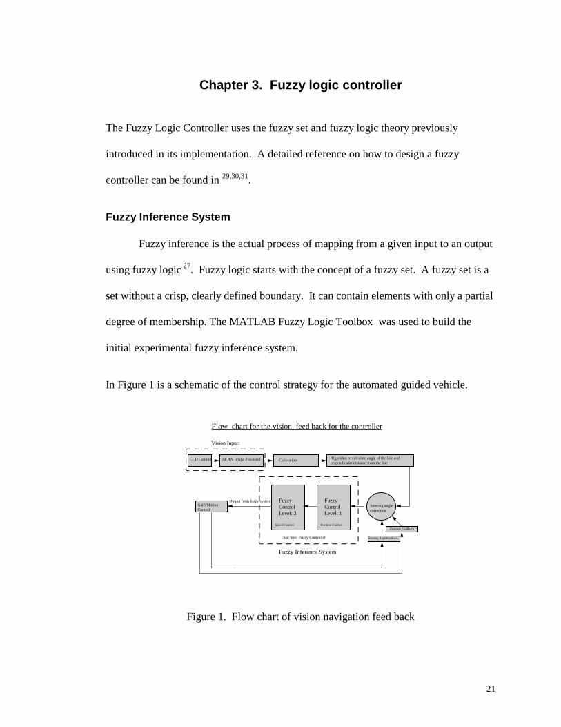
In Figure 1 is a schematic of the control strategy for the automated guided vehicle.
CCD Camera ISCAN Image Processor Calibration Algorithm to calculate angle of the line andperpendicular distance from the line
Steering anglecorrection
Galil Motion Control
Steering AngleFeedback
Output from fuzzy system:
Vision Input:
FuzzyControlLevel: 1
FuzzyControlLevel: 2
Flow chart for the vision feed back for the controller
Fuzzy Inferance System
Dual level Fuzzy Controller
Position ControlSpeed ControlPosition Feedback
Figure 1. Flow chart of vision navigation feed back
22
The fuzzy inference process consists of following steps:
Fuzzy Set Definition
Fuzzification
Rule Base
Fuzzy Operators
Implication
Aggregation
Defuzzification
Fuzzy Set Definition
The universe of discourse is identified and fuzzy sets are defined. The definition
of these sets requires expert knowledge of the control system. The most common shape
of membership functions is triangular, although trapezoidal and bell curves are also
used, but the shape is generally less important than the number of curves and their
placement. From three to seven curves are generally appropriate to cover the required
range of an input value (universe of discourse).
The shape of the membership function is also determined at this step. In this
application a triangular membership function is used. The reason behind this is that
they are easier to represent and implement, as a result the complexity of the problem is
reduced. The fuzzy set definition is more important than the shape of the membership
function.
23
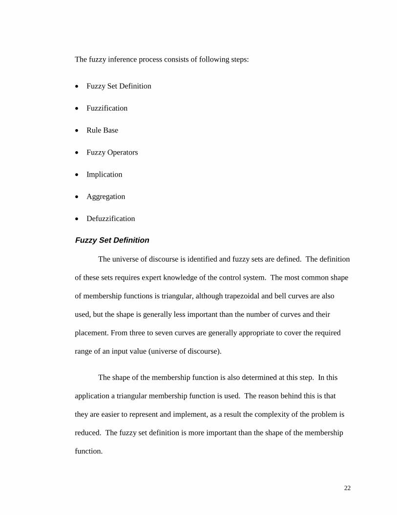
Input fuzzy sets
The first level of the fuzzy system has two inputs, �error and derror. These inputs
are resolved into a number of different fuzzy linguistic sets. For �error, there are
seven fuzzy sets. The scale for this input is -20 to 20
Fuzzy Set Description
a-3 Extreme left
a-2 Left
a-1 Soft left
a Zero
a1 Soft right
a2 Right
a3 Extreme right
Table 1 Input fuzzy sets
Figure 2. Input fuzzy sets (angle error)
Figure 2 shows the input membership functions for angle error ae:
24
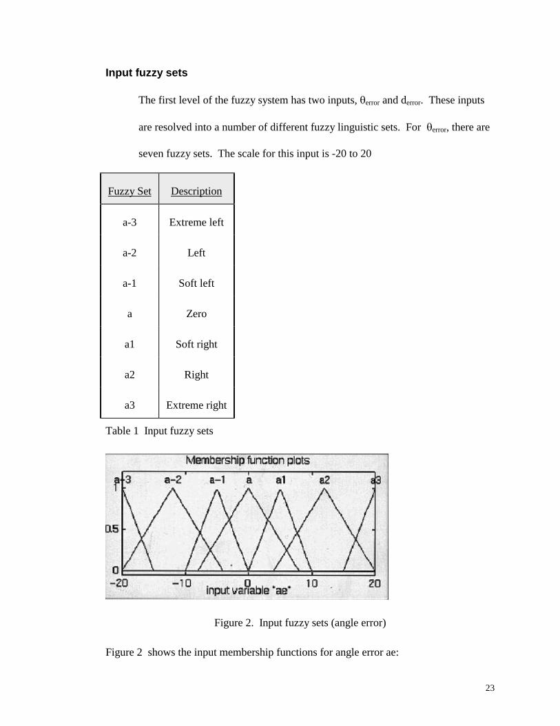
while derror also has five sets: Scale for this input is -30 inches to 30 inches
Fuzzy Set Description
d-2 Far left
d-1 Left
d Zero
d1 Right
d2 Far right
Table 2 Input fuzzy sets
Figure 3. Input fuzzy sets (distance error)
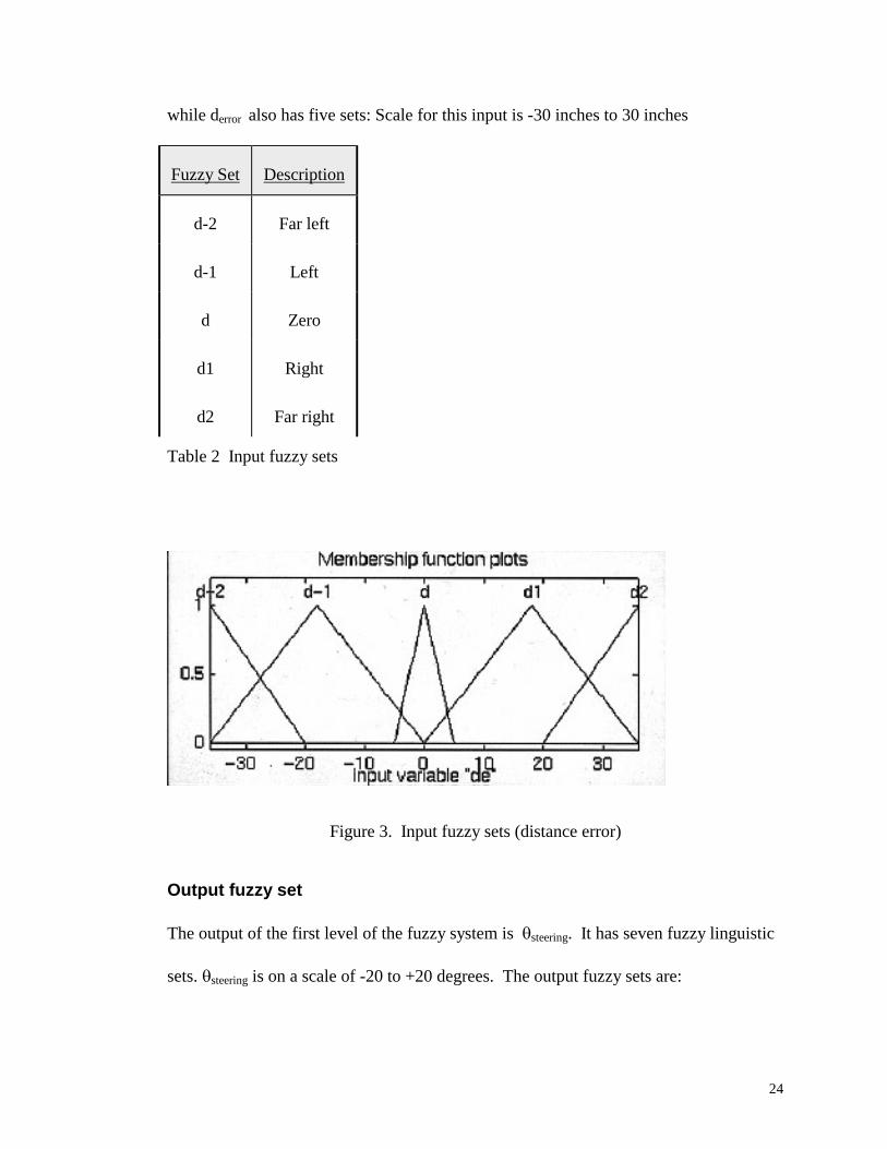
Output fuzzy set
The output of the first level of the fuzzy system is �steering. It has seven fuzzy linguistic
sets. �steering is on a scale of -20 to +20 degrees. The output fuzzy sets are:
25
Fuzzy Set Description
BP Big positive
MP Medium positive
SP Small positive
ZE Zero
SN Small negative
MN Medium negative
BN Big negative
Table 3 Output fuzzy sets
Figure 4. Output fuzzy sets (corrected steering angle)
Figure 4 shows the output membership functions for steering angle correction st:
26
Fuzzification
The input data (crisp data) is fuzzified according to the membership functions.
The fuzzified input is the degree to which each part of the antecedent has been satisfied
for each rule.
Rule Base
The way one develops control rules depends on whether or not the process can
be controlled by a human operator. If the operator's knowledge and experience can be
explained in words, then linguistic rules can be written immediately. If the operator's
skill can keep the process under control, but this skill cannot be easily expressed in
words, then control rules may be formulated based on the observation of operator's
actions in terms of the input - output operating data. However, when the process is
exceedingly complex, it may not be controllable by a human expert. In this case, a
fuzzy model of the process is built and the control rules are derived theoretically. It
should be noted however, that this approach is quite complicated and has not yet been
fully developed. Therefore the FLC is ideal for complex ill - defined systems that can
be controlled by a skilled human operator without the knowledge of their underlying
dynamics. In such cases an FL controller is quite easy to design and implementation is
less time consuming than for a conventional controller.
Determination of control rules remains a problem. Generally there are three
possible methods described as follows.
1. The method based on a fuzzy model of the process.

27
The relation between inputs and outputs can be expressed using linguistic
descriptions. This description is referred to as the fuzzy model of the system and
takes the form of conditional statements. Based on this model the optimal set of
control rules can be obtained 32.
2. The method based on the operator's experience and/or the control engineer's
knowledge.
These control rules are similar to rules formed by the human decision process.
This case is used in formulation of rules for the purpose of this controller. This
makes the rule formulation straightforward. In a man - machine interaction rules
can also be formed according to the operator's control actions.
3. The method based on learning
A FLC can be developed which can learn from a good or a bad experience.
Such a controller was first proposed by Mamdani in 1979.
In this case the rules were expressed linguistically with the help of human
logical decision making process. These rules can be appended along the way as the
human expertise increases.
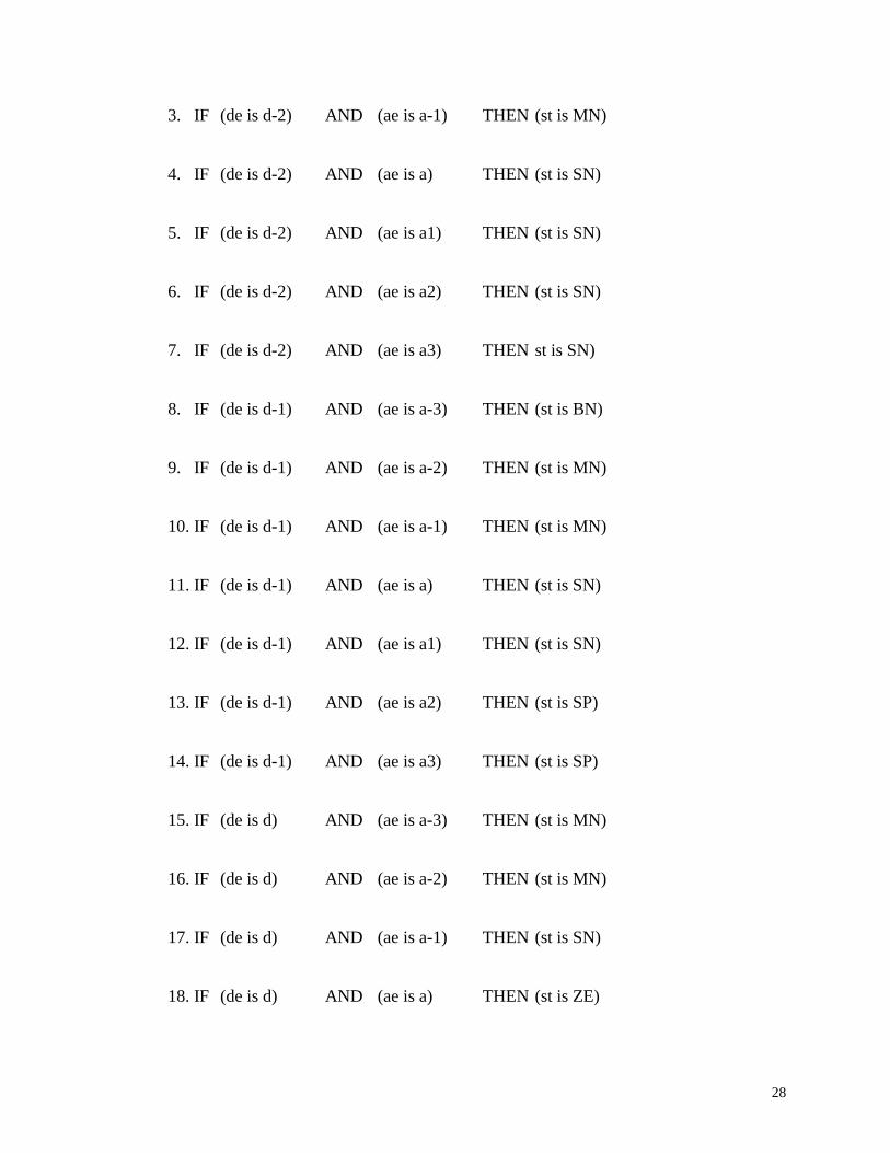
Following are the rules used for the control expressed as IF THEN rules:
1. IF (de is d-2) AND (ae is a-3) THEN (st is BN)
2. IF (de is d-2) AND (ae is a-2) THEN (st is BN)
28
3. IF (de is d-2) AND (ae is a-1) THEN (st is MN)
4. IF (de is d-2) AND (ae is a) THEN (st is SN)
5. IF (de is d-2) AND (ae is a1) THEN (st is SN)
6. IF (de is d-2) AND (ae is a2) THEN (st is SN)
7. IF (de is d-2) AND (ae is a3) THEN st is SN)
8. IF (de is d-1) AND (ae is a-3) THEN (st is BN)
9. IF (de is d-1) AND (ae is a-2) THEN (st is MN)
10. IF (de is d-1) AND (ae is a-1) THEN (st is MN)
11. IF (de is d-1) AND (ae is a) THEN (st is SN)
12. IF (de is d-1) AND (ae is a1) THEN (st is SN)
13. IF (de is d-1) AND (ae is a2) THEN (st is SP)
14. IF (de is d-1) AND (ae is a3) THEN (st is SP)
15. IF (de is d) AND (ae is a-3) THEN (st is MN)
16. IF (de is d) AND (ae is a-2) THEN (st is MN)
17. IF (de is d) AND (ae is a-1) THEN (st is SN)
18. IF (de is d) AND (ae is a) THEN (st is ZE)
29
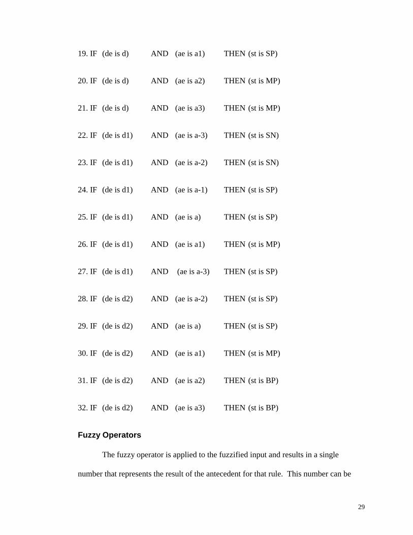
19. IF (de is d) AND (ae is a1) THEN (st is SP)
20. IF (de is d) AND (ae is a2) THEN (st is MP)
21. IF (de is d) AND (ae is a3) THEN (st is MP)
22. IF (de is d1) AND (ae is a-3) THEN (st is SN)
23. IF (de is d1) AND (ae is a-2) THEN (st is SN)
24. IF (de is d1) AND (ae is a-1) THEN (st is SP)
25. IF (de is d1) AND (ae is a) THEN (st is SP)
26. IF (de is d1) AND (ae is a1) THEN (st is MP)
27. IF (de is d1) AND (ae is a-3) THEN (st is SP)
28. IF (de is d2) AND (ae is a-2) THEN (st is SP)
29. IF (de is d2) AND (ae is a) THEN (st is SP)
30. IF (de is d2) AND (ae is a1) THEN (st is MP)
31. IF (de is d2) AND (ae is a2) THEN (st is BP)
32. IF (de is d2) AND (ae is a3) THEN (st is BP)
Fuzzy Operators
The fuzzy operator is applied to the fuzzified input and results in a single
number that represents the result of the antecedent for that rule. This number can be
30
then applied to the output membership function. The inputs to the fuzzy operator are
two or more membership values from fuzzified input variables.
In the controller presented we use a AND operator (product).
Implication
The implication method is defined as shaping of the consequent (a fuzzy set)
based on the antecedent (a single number). The input for the implication process is a
single number given by the antecedent, and the output is a fuzzy set.
The controller presented in this research uses an AND (product) implication
which scales the output fuzzy set.
31
Aggregation
Aggregation is the method for unifying the outputs of each rule by joining the
parallel threads. In this process all the output fuzzy sets from each rule are united into
one fuzzy set.
The SUM ( simple sum of each rule's output) type of aggregation is used in this
controller.
Defuzzification
The input for defuzzification is the fuzzy set (the aggregate output fuzzy set) and
the output is a crisp number. Defuzzification can be obtained using three known ways:
The mean of maximum method
The maximizing decision
The center of gravity method
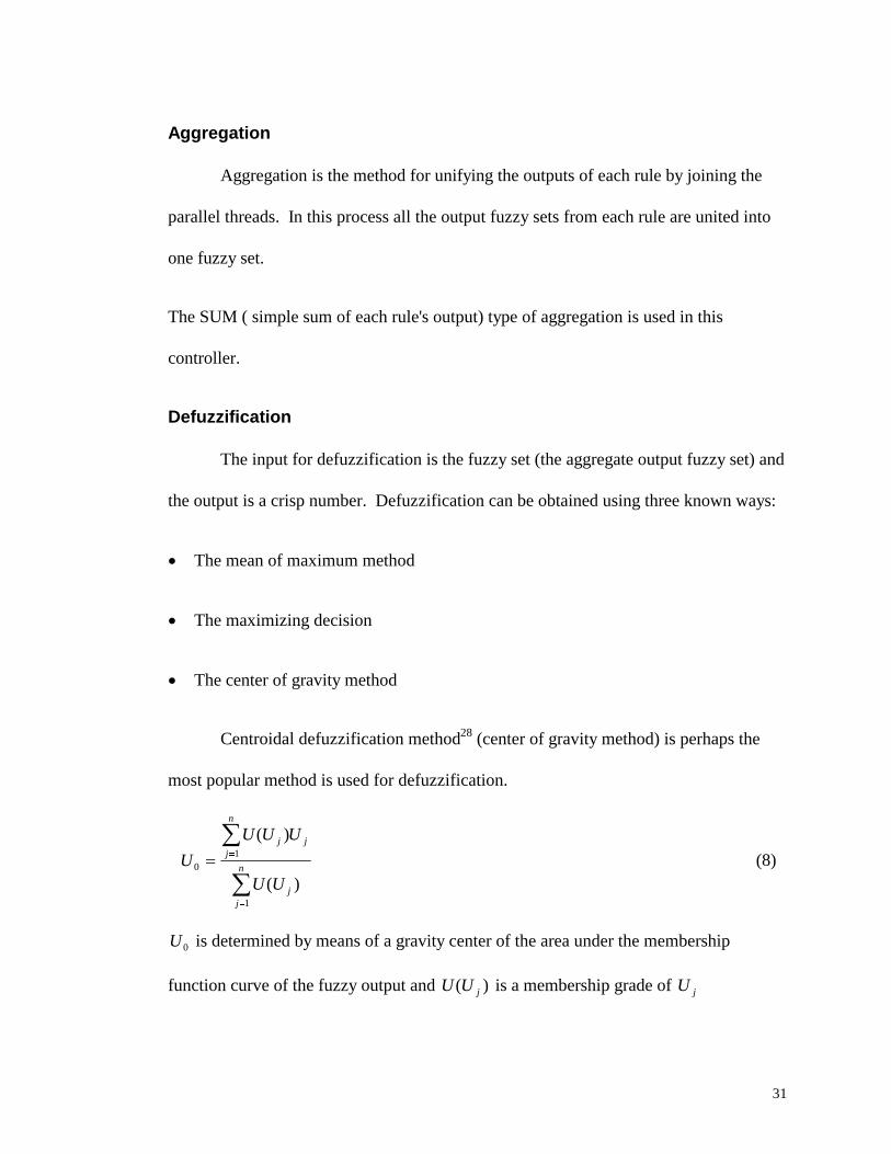
Centroidal defuzzification method28 (center of gravity method) is perhaps the
most popular method is used for defuzzification.
U
U U U
U U
j jj
n
jj
n01
1
��
�
�
�
( )
( ) (8)
U0 is determined by means of a gravity center of the area under the membership
function curve of the fuzzy output and U U j( ) is a membership grade of U j
32
Figure 5. Fuzzy centroidal defuzzification
Figure 5 shows how the fuzzy implication works and the center of gravity
defuzzification.
33
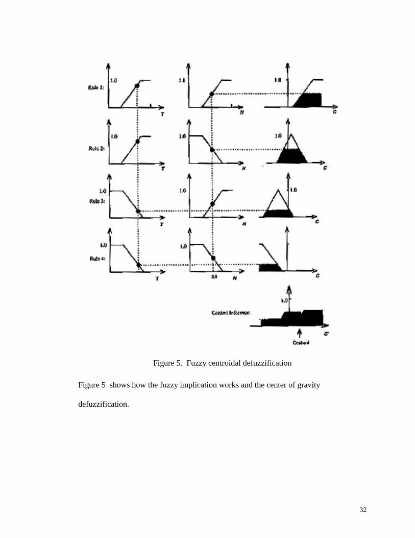
Figure 6. Fuzzy rule base for a particular input
34
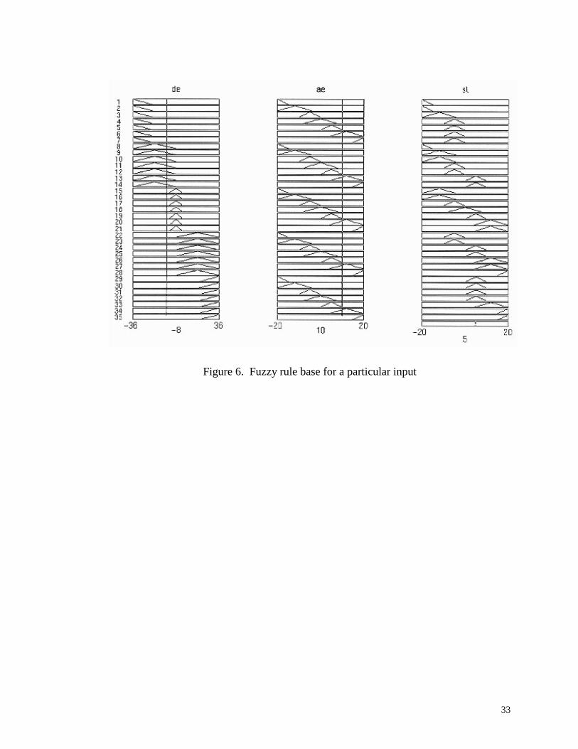
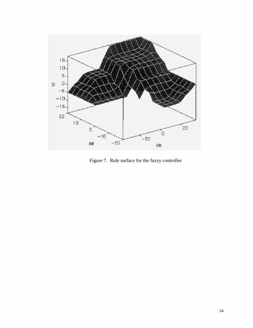
Figure 7. Rule surface for the fuzzy controller

35
Disadvantages of FLC
Although FLC provides the tools to incorporate human expert knowledge and
experience in automatic control systems, there are two important disadvantages:
Because a FL controller is a model-free estimator, it is difficult to develop a
model that can prove the stability of a fuzzy control system. One solution is to use
conventional control systems in conjunction with fuzzy systems to ensure stability.
Tuning of an FL controller is still an open problem for which no known
analytical technique presently exists. Therefore, tuning must be accomplished by a trial
and error procedure.
36
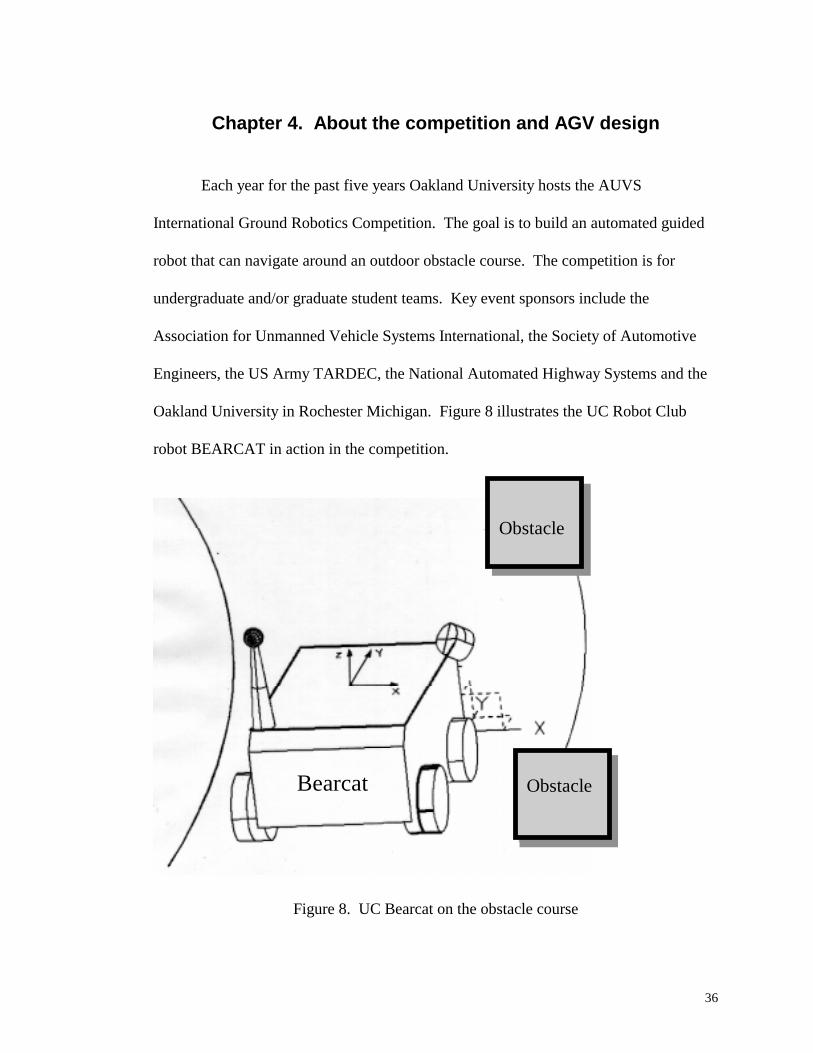
Chapter 4. About the competition and AGV design
Each year for the past five years Oakland University hosts the AUVS
International Ground Robotics Competition. The goal is to build an automated guided
robot that can navigate around an outdoor obstacle course. The competition is for
undergraduate and/or graduate student teams. Key event sponsors include the
Association for Unmanned Vehicle Systems International, the Society of Automotive
Engineers, the US Army TARDEC, the National Automated Highway Systems and the
Oakland University in Rochester Michigan. Figure 8 illustrates the UC Robot Club
robot BEARCAT in action in the competition.
Bearcat
Obstacle
Obstacle
Figure 8. UC Bearcat on the obstacle course
37
Objective
The objective of the competition is to promote research for automated guided
vehicles which can navigate ( vision and sonar navigation ) in between two lines (
continuous and dashed ) on the ground. These vehicles should also have the capacity to
detect and avoids obstacles in their path.
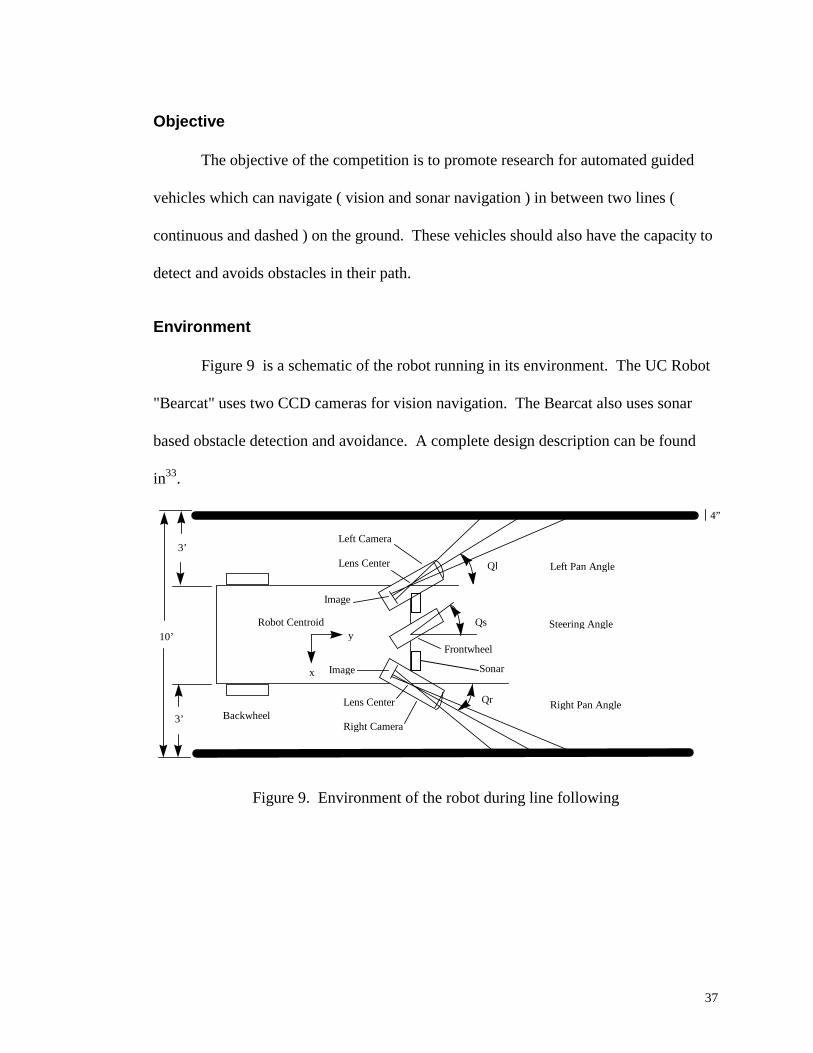
Environment
Figure 9 is a schematic of the robot running in its environment. The UC Robot
"Bearcat" uses two CCD cameras for vision navigation. The Bearcat also uses sonar
based obstacle detection and avoidance. A complete design description can be found
in33.
4”
Backwheel
Robot Centroid
x
y
Lens Center
Right Camera
Right Pan Angle
Left Pan Angle
Left Camera
Lens Center
Frontwheel
Steering Angle10’
3’
3’
Ql
Qs
Qr
Image
Image Sonar
Figure 9. Environment of the robot during line following
38
Chapter 5. Control
Vision guidance and data input
The purpose of the vision guidance is to guide the robot to follow the line using
a digital CCD camera. To do this, the camera needs to be calibrated. Camera
calibration 34 is a process to determine the relationship between a given 3-D coordinate
system (world coordinates) and the 2-D image plane a camera perceives (image
coordinates). More specifically, it is to determine the camera and lens model
parameters that govern the mathematical or geometrical transformation from world
coordinates to image coordinates based on the known 3-D control field and its image.
The CCD camera digitizes the line from 3-D coordinate system to 2-D image system.
Since the process is autonomous, the relationship between the 2-D system and the 3-D
system has to be accurately determined so that the robot can follow the line. The
objective of this section is to show how a model was developed to calibrate the vision
system so that, given any 2-D image coordinate point, the system can mathematically
compute the corresponding ground coordinate point. The X and Y (the Z is constant)
coordinates of two ground points are then computed from which the angle and the
perpendicular distance of the line with respect to the centroid of the robot are
determined.
The vision system was modeled by the following equations.
xPI = A11 xg + A12yg + A13zg + A14 (9)
yPI = A21xg + A22yg + A23zg + A24 (10)
39
where Anm are coefficients, xPI and yPI are x and y image coordinates, and xg, yg, and zg
are the ground coordinates. In transforming the ground coordinate points to the image
coordinate points the following transformation operations occur on the points: scaling,
translation, rotation, perspective, and projective. Solving for the transformation
parameters to obtain the image and ground coordinate relationship is a difficult task.
Fortunately, in the model equations given above, the transformation parameters are
imbedded into the coefficients. To compute the coefficients, a calibration device was
built to obtain 12 data points. With the 12 points, a matrix equation was yielded as
shown below:
XPI = CA1k (11)
YPI = CA2k (12)
where
C XPI YPI
xg yg zg
xg yg zg
xg yg zg
xPI
xPI
xPI
yPI
yPI
yPI
A
A
A
A
A
A
A
A
A
A
k k�
�
��������
�
�
��������
�
�
��������
�
�
��������
�
�
��������
�
�
��������
�
�
�����
�
�
�����
�
�
����
�
�
����
1 1 1
2 2 2
12 12 12
1
2
12
1
2
12
11
12
13
14
2
1
1
1
1
21
22
23
24
. . . .
. . . .
. . . .
. ;.
.
.
;.
.
.
; ;
Equations (11) and (12) consist of 12 linearly independent equations and four
unknowns, the least-square regression method is applied to yield a minimum mean-
square error solution for the coefficients. Below are the equations for the solution:
A1K = (CTC)-1CTXPI (13)
A2K = (CTC)-1CTYPI (14)
40
Given an image coordinate xPI and yPI, and z ground coordinate (the z
coordinate of the points with respect to the centroid of the robot is maintained constant
since the robot is run on a flat surface in this model) the corresponding xg and yg ground
coordinates are computed as indicated by the following matrix equations.
g
g
x
yQ
�
���
�
��� �
�1� (15)
where
Q A A
A AB
xPI A A zyPI A A z
g
g
�
��
�
�� �
� �
� �
���
�
���
11 12
21 22
14 13
24 23
;( )
( )
Note that equation (9) and (15) can be modified to accommodate the
computation of zg when an elevation of the ground surface is considered.
The image processing of the physical points is done by the ISCAN tracking
device, which returns the centroid of the brightest or darkest region in a computer
controlled windows and returns its X and Y coordinates. Two points on the line are
windowed and their corresponding coordinates are computed as described above. From
the computed x and y ground coordinates of the points, the angle of the line with respect
to the centroid of the robot is computed from simple trigonometric relationship. In the
next section, we shall show how the angle of the line just computed is used with other
parameters to model the steering control of the robot with a fuzzy logic controller.
41
y
P a th w ithd
R o b o t
��
G iven a cros s track e rror , d , and a ttitude e rro r, � , thecon tro l p ro b lem is to de te rm ine how to m a ke both d (t) and � ( t)app roach 0 .
P a th w ith �� 0
0
P a th w ithd 0
b o thand
�� 0
x
d
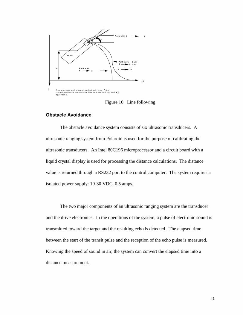
Figure 10. Line following
Obstacle Avoidance
The obstacle avoidance system consists of six ultrasonic transducers. A
ultrasonic ranging system from Polaroid is used for the purpose of calibrating the
ultrasonic transducers. An Intel 80C196 microprocessor and a circuit board with a
liquid crystal display is used for processing the distance calculations. The distance
value is returned through a RS232 port to the control computer. The system requires a
isolated power supply: 10-30 VDC, 0.5 amps.
The two major components of an ultrasonic ranging system are the transducer
and the drive electronics. In the operations of the system, a pulse of electronic sound is
transmitted toward the target and the resulting echo is detected. The elapsed time
between the start of the transit pulse and the reception of the echo pulse is measured.
Knowing the speed of sound in air, the system can convert the elapsed time into a
distance measurement.
42
The drive electronics has two major categories - digital and analog. The digital
electronics generate the ultrasonic frequency. A drive frequency of 16 pluses per second
at 52 kHz is used in this application. All the digital functions are generated by the Intel
microprocessor. The analog functionality is provided by the Polaroid integrated circuit.
The operating parameters such as the transmit frequency, pulse width, blanking time and
the amplifier gain are controlled by polakit, a developers software provided by Polaroid.
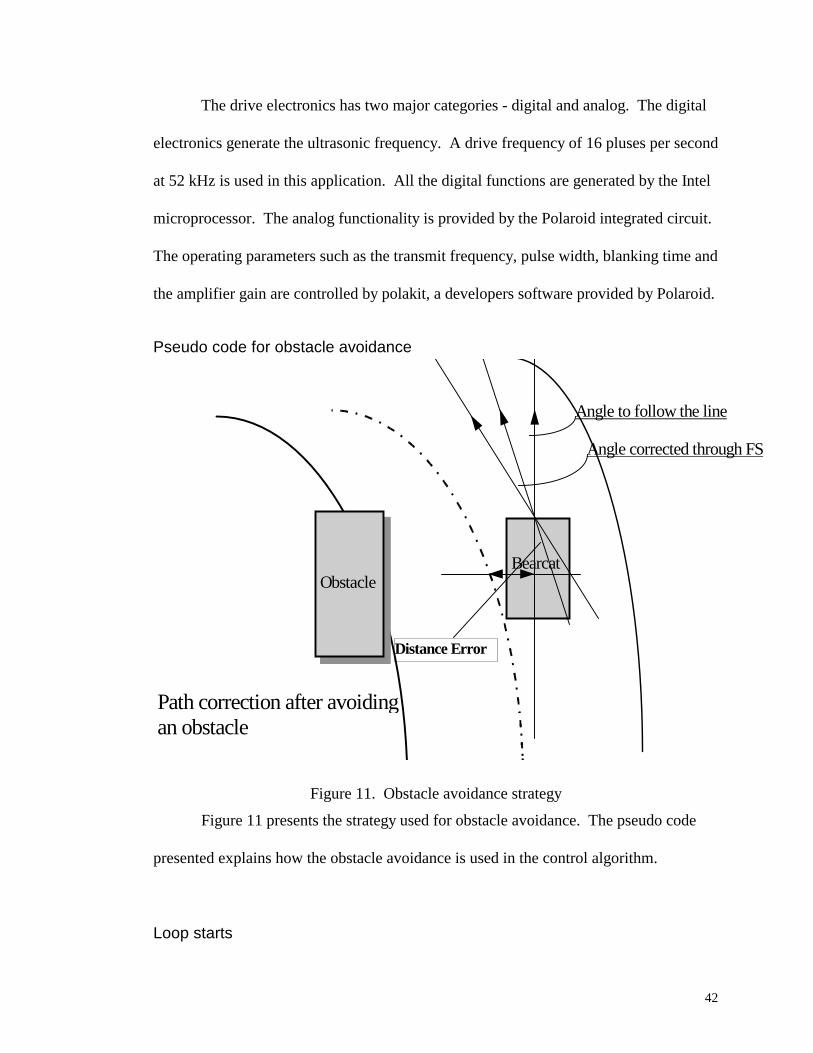
Pseudo code for obstacle avoidance
Bearcat
Angle to follow the line
Angle corrected through FS
Obstacle
Path correction after avoidingan obstacle
Distance Error
Figure 11. Obstacle avoidance strategy
Figure 11 presents the strategy used for obstacle avoidance. The pseudo code
presented explains how the obstacle avoidance is used in the control algorithm.
Loop starts

43
Get input from vision input ( Scanning device )
Process and validate input.
Calculate the distance error and the angle error.
Check for obstacle on the right and left
If the obstacle is less than three feet and greater than two feet
Change the distance error value
If the distance error is negative and the obstacle is on the
right
Increase the distance error by 10 inches
If the distance error is negative and the obstacle is on the
left
Reduce the distance error by 5 inches
If the distance error is positive and the obstacle is on the
right
Reduce the distance error by 5 inches
If the distance error is positive and the obstacle is on the
left
Increase the distance error by 10 inches
Input the distance error and angle error to the fuzzy controller
Steer the robot according to the output steering angle.
If the obstacle is less than two feet and greater than one feet
If the obstacle is on the left steer the robot to right by 10 degrees
Else steer the robot to the left by 10 degrees

44
If the obstacle is within one feet
If the obstacle is on the left steer the robot to right by 20 degrees
Else steer the robot to the left by 20 degrees
End Loop
The strategy for obstacle avoidance, in short, is to modify the distance error
input to the fuzzy controller and use the same fuzzy controller again to compute the
corrected motion direction. This way redesign of a separate controller for obstacle
avoidance is avoided. The pseudo code explains how and by what amount the distance
error should be modified.
45
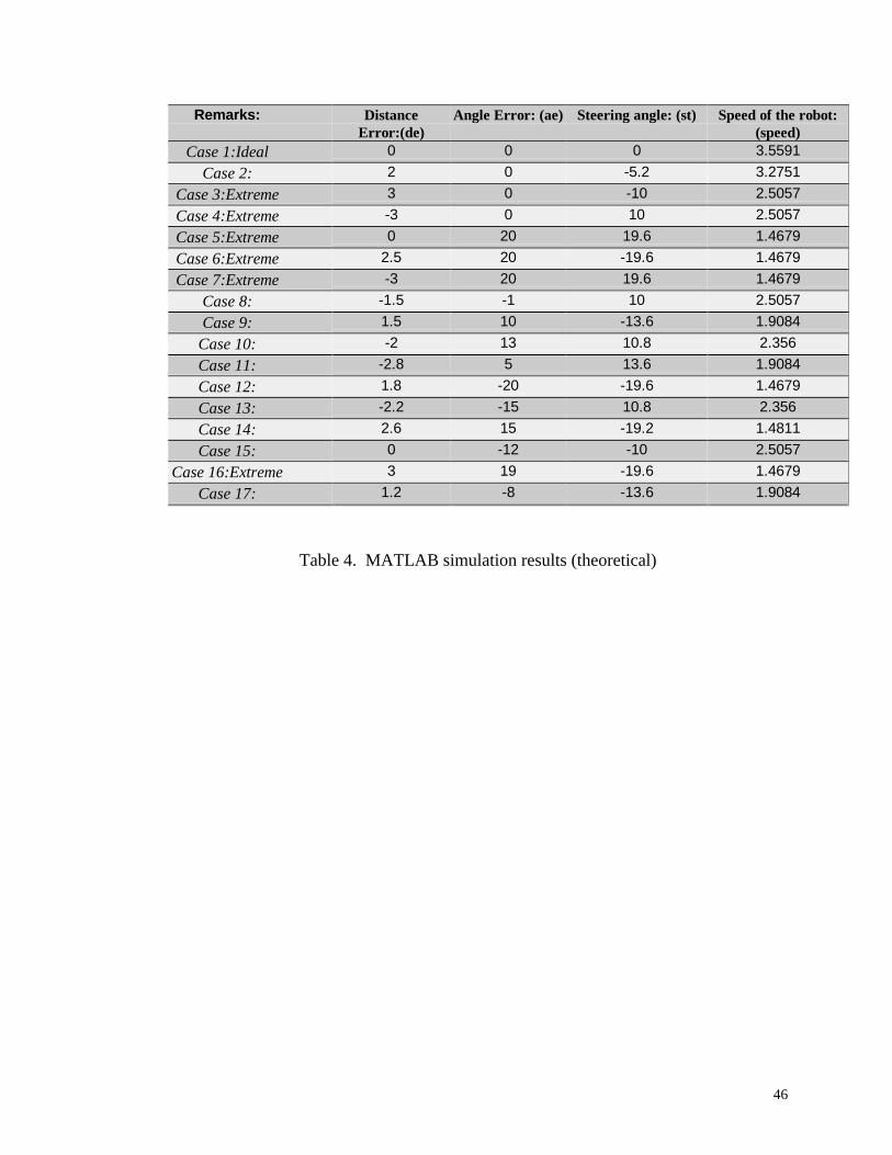
Chapter 6. Results
The testing of the dual level fuzzy system controller explained in Chapter 3 was
done in two steps. First, a theoretical simulation was run using the MATLAB fuzzy tool
box. The input for this simulation was generated using theoretical test cases. The inputs
to the MATLAB batch file which was used to run the simulation (M-file) were �error and
derror. The outputs were �steering and the speed of the robot. Seventeen cases were
considered. Results of the simulation are shown in Table 1 . Appendix C has the code
for the M-file. Note that the results appear reasonable for both angle and speed. The
results of these simulations encouraged further tests using a real life scenario. As a
result the model was also implemented on the mobile robot, which is scheduled to take
part in a nation wide obstacle avoidance and path following competition in June '97.
46
Remarks: DistanceError:(de)
Angle Error: (ae) Steering angle: (st) Speed of the robot:(speed)
Case 1:Ideal 0 0 0 3.5591
Case 2: 2 0 -5.2 3.2751
Case 3:Extreme 3 0 -10 2.5057
Case 4:Extreme -3 0 10 2.5057
Case 5:Extreme 0 20 19.6 1.4679
Case 6:Extreme 2.5 20 -19.6 1.4679
Case 7:Extreme -3 20 19.6 1.4679
Case 8: -1.5 -1 10 2.5057
Case 9: 1.5 10 -13.6 1.9084
Case 10: -2 13 10.8 2.356
Case 11: -2.8 5 13.6 1.9084
Case 12: 1.8 -20 -19.6 1.4679
Case 13: -2.2 -15 10.8 2.356
Case 14: 2.6 15 -19.2 1.4811
Case 15: 0 -12 -10 2.5057
Case 16:Extreme 3 19 -19.6 1.4679
Case 17: 1.2 -8 -13.6 1.9084
Table 4. MATLAB simulation results (theoretical)
47
Matlab Simulations
Simulations were run using artificially made-up and real-time data collected
using the robots vision system and the ultrasonic obstacle avoidance system. Five cases
were considered for this study. The collected data was used as an input to the fuzzy
inference system implemented in C programming language and MATLAB was used to
provide graphics support. Each case from case one to five was made more difficult for
the controller by introducing noise in the input data in form of input data variations
caused by loss of vision ( loss of track of line) and obstacles in the path.
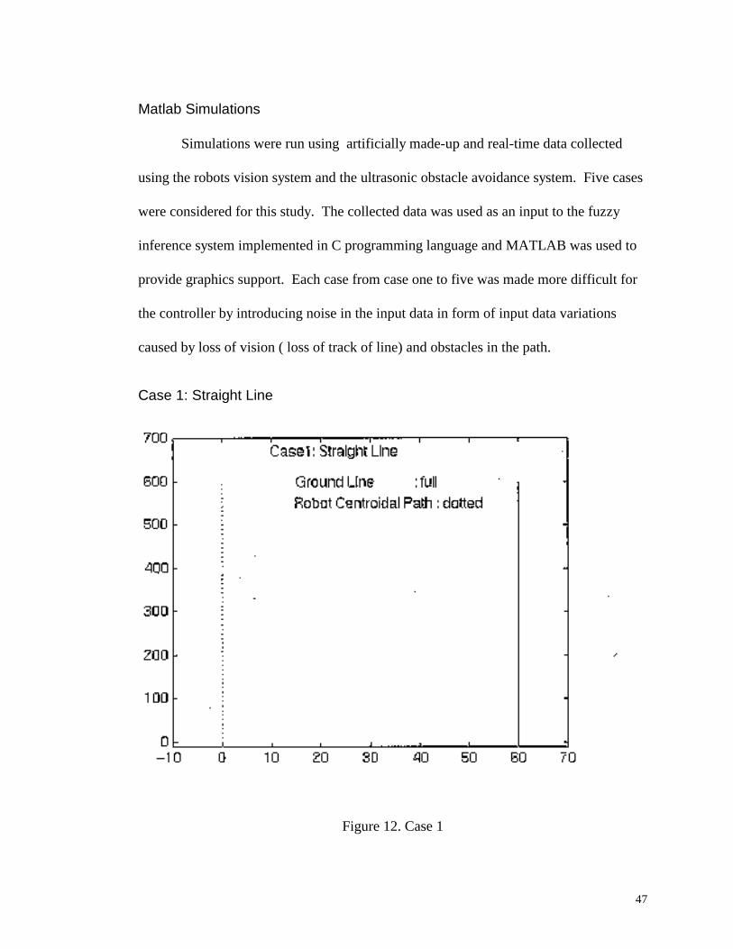
Case 1: Straight Line
Figure 12. Case 1

48
The objective of this case was to test if the controller handles a simple case as
straight line following. The actual line is represented by a solid straight line and the
actual path of the robot ( the centroidal path ) is represented by the dotted line in all the
cases. The resultant output of this simulation is presented in Figure 12. The output
indicates a successful line following.
49
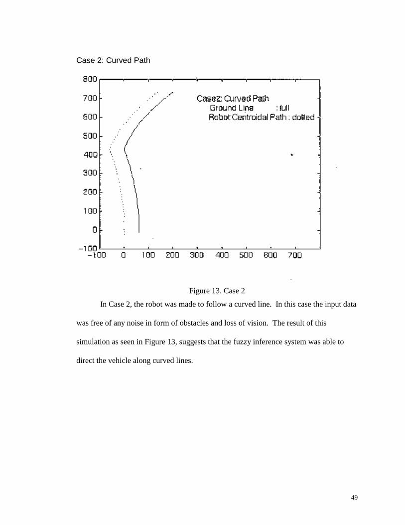
Case 2: Curved Path
Figure 13. Case 2
In Case 2, the robot was made to follow a curved line. In this case the input data
was free of any noise in form of obstacles and loss of vision. The result of this
simulation as seen in Figure 13, suggests that the fuzzy inference system was able to
direct the vehicle along curved lines.
50
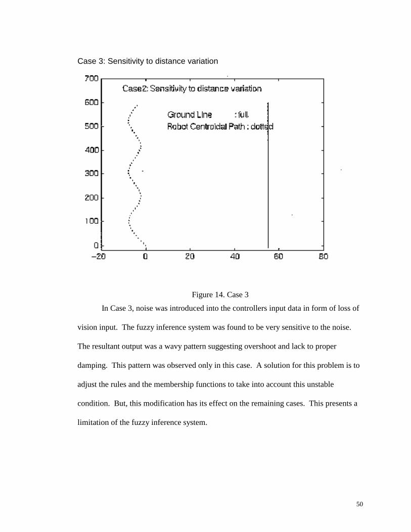
Case 3: Sensitivity to distance variation
Figure 14. Case 3
In Case 3, noise was introduced into the controllers input data in form of loss of
vision input. The fuzzy inference system was found to be very sensitive to the noise.
The resultant output was a wavy pattern suggesting overshoot and lack to proper
damping. This pattern was observed only in this case. A solution for this problem is to
adjust the rules and the membership functions to take into account this unstable
condition. But, this modification has its effect on the remaining cases. This presents a
limitation of the fuzzy inference system.
51
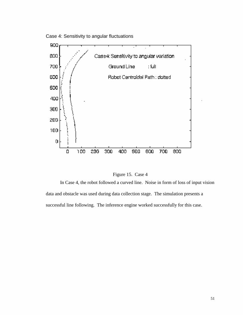
Case 4: Sensitivity to angular fluctuations
Figure 15. Case 4
In Case 4, the robot followed a curved line. Noise in form of loss of input vision
data and obstacle was used during data collection stage. The simulation presents a
successful line following. The inference engine worked successfully for this case.
52
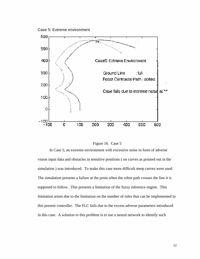
Case 5: Extreme environment
Figure 16. Case 5
In Case 5, an extreme environment with excessive noise in form of adverse
vision input data and obstacles in sensitive positions ( on curves as pointed out in the
simulation ) was introduced. To make this case more difficult steep curves were used.
The simulation presents a failure at the point when the robot path crosses the line it is
supposed to follow. This presents a limitation of the fuzzy inference engine. This
limitation arises due to the limitation on the number of rules that can be implemented in
this present controller. The FLC fails due to the excess adverse parameters introduced
in this case. A solution to this problem is to use a neural network to identify such

53
extreme conditions and use dedicated fuzzy inference engines for each case identified
by the neural network. This solution has been discussed on in Chapter 7.
54
Chapter 7. Conclusion and Recommendations
Conclusion
The design and implementation of a modular fuzzy logic based controller for an
autonomous mobile robot for line following along an obstacle course has been
presented. The control algorithm for this application is based on vision navigation. The
development of the FLC controller was done after a detail study of the autonomous
guided vehicle and its environment. A rule base was generated using expert system
knowledge. Fuzzy membership functions and fuzzy sets were developed. The FLC
model was first tested on the MATLAB fuzzy logic toolkit with some special cases.
The FLC was then implemented in C programming language and a number of tests were
run to analyze the stability and response of the system under fuzzy control in a real life
scenario. Tuning of the system in form of adjusting the membership functions and the
rules was done to improve the stability of the FLC.
The fuzzy logic control is a very flexible and robust soft computing tool for
control. The number of variants involved in the current application present a challenge
for any type of control system. A fuzzy logic control was selected, as a soft computing
solution for this problem keeping in mind its robustness and flexibility. The
performance of the robot was studied with simulations for five different cases selected
for the study. The FLC shows good stability and response for three of the cases. The
problem at hand seems to be a complex problem for just one inference engine to handle.
This limitation arises due to the limit on the number of rules and membership functions
55
that can be used in a single inference engine. A better system performance can be
obtained if a neuro-fuzzy approach is used. The environment in which the robot runs
should be divided into a number of specific classes according to input data. The control
system model will contain a neural net to identify and classify input data, which will
finally fire the right inference engine for the input data class. From the results obtained
in the MATLAB simulation and the preliminary testing of the model on the robot, it can
be concluded that the model presented, can be reliably and successfully implemented
permanently on the robot.
Fuzzy logic has been proven to be a excellent solution to control problems where
the number of rules for a system are finite and which can be easily established. In this
application an infinite number of rules can be established. The fuzzy control in a way
acts as a learning system control, as it has the ability to learn from situations where it
fails. This learning is possible by increasing the number of rules in the system. In this
way the system can keep on learning until it becomes a perfect system. No system is
perfect in the onset; as such the necessary refinements and modifications will be made
to make the UC Bearcat a competitive mobile robot.
56
Future Recommendations
The FLC has proven to be a robust controller for this system. FLC can be
successfully implemented in systems which need robust performance. The FLC is
stable under all the cases discussed in Chapter 6. Tuning of the FLC is a challenging
task and needs an expert knowledge. The total error of the control loop can be reduced
according to the needs of a system by tuning the FLC. The tuning process is the
modification of fuzzy sets and fuzzy rule base. The shape of the membership function
has a negligible effect on the final stability of the system. Future research should be
directed to the development of an easier tuning method for the fuzzy system. Also,
alpha cut and clustering algorithms could be used for better performance of the fuzzy
engine.
It was observed during this study that, this particular control problem had some
special cases which could be eventually handled more effectively by separate fuzzy
inference engines. A neuro-fuzzy approach should be tried with this problem. A neural
network should be used to identify special cases which arise during the motion of the
robot on the path. Then a separate FLC should be used to control each case
independently. This will improve the performance of the system with regards to the
stability aspect.
Future considerations might also include experimenting with different fuzzy
implications and operators for this particular application. This fuzzy approach can also

57
be used in other aspects of the system such as safety, error anticipation and handling and
fault reporting.
58
References
[1] P. F. Muir and C. P. Neuman, ‘Kinematic Modeling of Wheeled Mobile Robots,’
Journal of Robotic Systems, 4(2), 1987, pp. 281-340
[2] E. L. Hall and B. C. Hall, Robotics: A User-Friendly Introduction, Holt,
Rinehart, and Winston, New York, NY, 1985, pp. 23.
[3] Z. L. Cao, S. J. Oh, and E. L. Hall, “Dynamic omni-directional vision for mobile
robots,” Journal of Robotic Systems, 3(1), 1986, pp. 5-17.
[4] Z. L. Cao, Y. Y. Huang, and E. L. Hall, “Region Filling Operations with Random
Obstacle Avoidance for Mobile Robots,” Journal of Robotics Systems, 5(2), 1988, pp.
87-102.
[5] S. J. Oh and E. L. Hall, “Calibration of an omni-directional vision navigation
system using an industrial robot,” Optical Engineering, Sept. 1989, Vol. 28, No. 9, pp.
955-962.
[6] R. M. H. Cheng and R. Rajagopalan, “Kinematics of Automated Guided Vehicles
with an Inclined Steering Column and an Offset Distance: Criteria for Existence of
Inverse Kinematic Solution,” Journal of Robotics Systems, 9(8), Dec. , 1992, 1059-
1081.
[7] M. P. Ghayalod, E. L. Hall, F. W. Reckelhoff, B. O. Mathews and M. A.
Ruthemeyer, “Line Following Using Omni-directional Vision,” Proc. of SPIE
59
Intelligent Robots and Computer Vision Conf., SPIE Vol. 2056, Boston, MA, 1993,
page 101.
[8] Kazuo Tanaka, “Design of Model-based Fuzzy Controller Using Lyapunov’s
Stability Approach and Its Application to Trajectory Stabilization of a Model Car,”
Theoretical Aspects of Fuzzy Control, John Wiley & sons, 1995. 2nd IEEE
conference on fuzzy system, San Francisco, CA, 1993, Inc, pp.31-50.
[9] C. V. Altrock et al., “Advanced fuzzy logic control technologies in automotive
applications”, Proceedings of 1st IEEE international Conference on Fuzzy Systems,
1992, pp. 835-842.
[10] L. A. Zadeh, "Outline of a new Approach to the Analysis of Complex Systems and
Decision Process", 1973 IEEE Transacions on Systems, Man and Cybernetics, v3,
pp 28-44.
[11] E. H. Mamdani, "Fuzzy Sets for Man - Machine Interaction ", 1977, IEEE
Transactions on Computer, v26, pp. 1182-1191.
[12] J. F. Baldwin and N. C. F. Guild, "Feasible Algorithms For Approximate
Reasoning Using Fuzzy Logic", 1980, Fuzzy Sets and Systems, v3, pp. 225-251..
[13] J. F. Baldwin and B. W. Pilsworth, "Axiomatic Approach For Approximate
Reasoning with Fuzzy Logic", 1980, Fuzzy Sets and Systems, v3, pp. 193-219
[14] J. B. Kiszka, M. M. Gupta and G. M. Trojan, "Multi Variable Fuzzy Controller
under Goedel's Implication", Fuzzy Sets and Systems, v34, pp. 301-321.
60
[15] Z. Cao and A. Kandel, "Applicability of some Fuzzy Implication Operators", 1989,
Fuzzy Sets and Systems, v31, pp. 151-186.
[16] A. Bardossy, L. Duckstein, "Fuzzy Rule based Modeling with Application to
Geophysical, Biological and Engineering Systems", 1995, CRC Press, New York,
pp.62-68.
[17] H. Hellendoorn, R. Palm, "Fuzzy Systems Technologies at Siemens R & D", 1994,
Fuzzy Sets and Fuzzy Systems, Vol. 63, pp. 245-269.
[18] M. Jamshidi, N. Vadiee, T. Ross, "Fuzzy Logic Control", 1993, PTR Prentice Hall,
Englewood Cliffs, New Jersey 07632, pp 89-101.
[19] P. King, E. Mamdani, "The application of Fuzzy Control Systems to Industrial
Process", 1977, Automatica, Vol. 3, pp. 235-242.
[20] R. Stenz, U. Kuhn, "Automation of a batch distillation column using Fuzzy and
Conventional Control", 1995 IEEE Transactions on Systems Technology, Vol. 3, pp.
171-176.
[21] T. Takahashi, M. Kitou, M. Asai, M. Kido, T. Chiba, J. Kawakami, Y. Matsui, "A
new voltage equipment using Fuzzy Inference", 1994, Electrical Engineering in
Japan, Vol. 114, pp. 18-32.
[22] C. von Altrock, Fuzzy Logic and NeuroFuzzy Applications Explained Prentice
Hall PTR, Englewood Cliffs, NJ, 07632, page 78.
61
[23] J. Yen, R. Langari, L. Zadeh, "Industrial applications of Fuzzy Logic and
Intelligent Systems", 1995, IEEE Press, IEEE Inc, New York, pp 08-09.
[24] T. Yamakawa, "Stabilization of an inverted pendulum by a high-speed Fuzzy
Logic Controller Hardware System", Fuzzy Sets and Systems, Vol. 32, pp. 161-180.
[25] Charles P. Coleman and Datta Godbole, University of California at Berkeley “A
Comparison of Robustness: Fuzzy Logic, PID, & Sliding Mode Control”, 1996, pp.06-
08
[26] Z. Yuzhou, R. McLauchlan, R. Challoo and S. Omar "Fuzzy Logic Control of a
four-link Robotic Manipulator in a Vertical Plane" Proceedings of the Artificial Neural
Networks in Engineering (ANNIE '96 ) Conference, held November 10-13, 1996, St.
Louis US, pp 198-200.
[27] J.-S. Roger Jang and Ned Gulley, Fuzzy Logic Toolbox For Use with
MATLAB , The MathWorks Inc. 1995, pp 90-92.
[28] Bart Kosko “Neural Networks and Fuzzy Systems- A Dynamical Systems
Approach To Machine Intelligence”, Prentice Hall, Englewood Cliffs, NJ 07632, pp 45-
67.
[29] N. Gulley "How To Design Fuzzy Logic Controllers" from Machine Design,
November 1992, page 26.
62
[30] Mark Kantrowitz, Erik Horstkotte, and Cliff Joslyn “The Internet fuzzy-logic FAQ
("frequently-asked questions") list” postings for comp.ai.fuzzy
URL:ftp.cs.cmu.edu:/user/ai/pubs/faqs/fuzzy/fuzzy_1.faq, 1996
[31] Kevin Self "Designing With Fuzzy Logic" from IEEE SPECTRUM, November
1990, Volume 105 pp 42-44.
[32] T. Takagi, M. Sugeno, "Fuzzy Identification of Systems and it's Application to
Modeling and Control", 1985, IEEE Transactions on Systems, Man, and Cybernetics,
V.SMC-15, pp. 116-132.
63
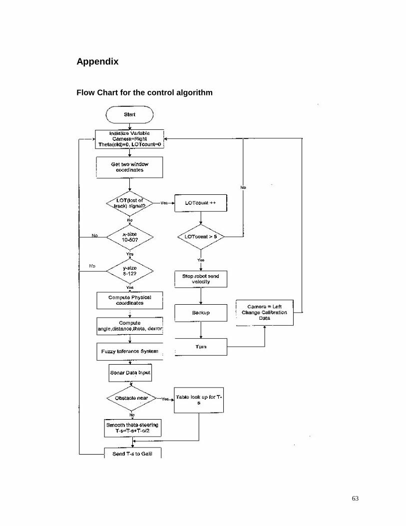
Appendix
Flow Chart for the control algorithm
64
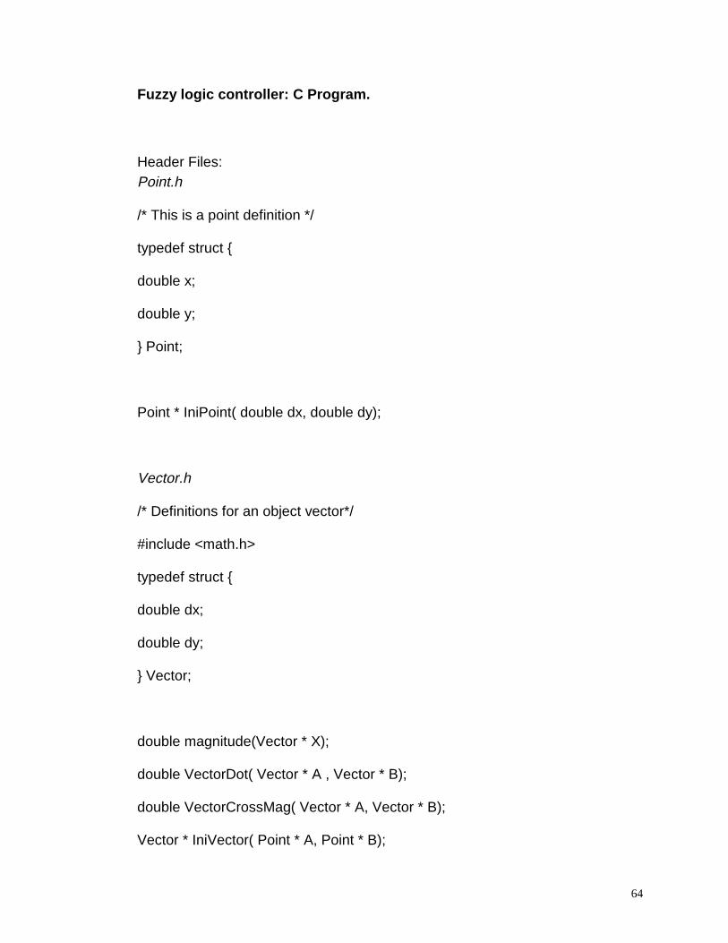
Fuzzy logic controller: C Program.
Header Files:Point.h
/* This is a point definition */
typedef struct {
double x;
double y;
} Point;
Point * IniPoint( double dx, double dy);
Vector.h
/* Definitions for an object vector*/
#include <math.h>
typedef struct {
double dx;
double dy;
} Vector;
double magnitude(Vector * X);
double VectorDot( Vector * A , Vector * B);
double VectorCrossMag( Vector * A, Vector * B);
Vector * IniVector( Point * A, Point * B);
65
Vector * UnitVector( Vector * N );
Vector * UnitVectorXaxis();
Vectors.h
#include "point.h"
#include "vector.h"
#include "fcontrol.h"
Fcontrol.h
/* header file for the fcontrol function..Fuzzy Controller.*/
#include "fuzzin.h"
double Fcontrol( double x, double phi);
Fuzzin.h
#include <stdio.h>
double fuzzin ( double x, double left, double mid, double right );
double SumMatrix ( int rules[][5], double state[][5] );
66
Main control code/* Using the point and the vector header files.*/
#include <stdio.h>
#include <stddef.h>
#include <alloc.h>
#include <string.h>
#include <math.h>
#include "vectors.h"
void main(){
FILE *data;
int count;
float distance;
double dx1, dy1, dx2, dy2, dx3, dy3, dx4, dy4, temp, temp1;
double phi, phi1, addangle, angle;
double test1, test2; /* debug values*/
double dist1, dist2, offset;
char buf[40];
Point * R1, * R2, * G1, * G2, * G1_old, * G2_old;
Vector * N1, * N2, * unitx;
/* Initialize variables */
67
count = 0; /* counter for number of cycles */
phi1 = 0;
R1 = (Point *) malloc(sizeof(Point)); /* Robot centroid*/
R2 = (Point *) malloc(sizeof(Point)); /* Robot Steering position */
G1 = (Point *) malloc(sizeof(Point)); /* Ground 1 */
G2 = (Point *) malloc(sizeof(Point)); /* Ground 2 */
G1_old = (Point *) malloc(sizeof(Point)); /* Old ground points */
G2_old = (Point *) malloc(sizeof(Point));
N1 = (Vector *) malloc(sizeof(Vector));
N2 = (Vector *) malloc(sizeof(Vector));
unitx = (Vector *) malloc(sizeof(Vector));
if( (data=fopen("data.dat","r")) == NULL )
puts("Can not find the file data.dat");
while( fgets(buf, 30, data) > 0 ){
/* To start with I have 8 point input Otherwise just 4 points */
if(count == 0){
sscanf( buf,"%lf %lf %lf %lf %lf %lf %lf %lf
",&dx1,&dy1,&dx2,&dy2,&dx3,&dy3,&dx4,&dy4);
R1 = IniPoint( dx1, dy1);
R2 = IniPoint( dx2, dy2);
68
}
else
sscanf( buf,"%lf %lf %lf %lf ",&dx3,&dy3,&dx4,&dy4);
G1 = IniPoint( dx3, dy3);
G2 = IniPoint( dx4, dy4);
N1 = IniVector( R1, R2);
N2 = IniVector( G1, G2);
temp = magnitude( N1 ) * magnitude( N2 );
temp1 = VectorCrossMag( N1, N2);
temp = temp1 / temp ;
phi = asin(temp);
/* Compute the addition angle */
unitx = UnitVectorXaxis();
temp = magnitude( N1 );
addangle = VectorCrossMag( unitx, N1);
addangle = addangle / temp;
addangle = asin(addangle);
addangle = addangle * 180 / 3.14;
printf("Input R1:%lf,%lf and R2:%lf,%lf",R1->x,R1->y,R2->x,R2-
>y);
69
printf("Input G1:%lf,%lf and G2:%lf,%lf \n",G1->x,G1->y,G2-
>x,G2->y);
printf("Angle computed is: %lf\n",phi*180/3.14);
// printf("AddAngle computed is: %lf\n",addangle);
/* Calculate distance error*/
/* Shift to local co-ordinate system and calculate the x distance with respect to
the last point */
/* Local Co-ordinates */
if(count != 0){
dist1 = sqrt( ((G2_old->x - R2->x) * (G2_old->x - R2->x)) +
((G2_old->y - R2->y) * (G2_old->y - R2->y)) );
// dist2 = ( G2_old->x - R1->x );
/* Distance is the mean x position */
// distance = (float) ((dist1 + dist2) / 2 );
distance = dist1;
// printf("Distance computed is: %lf ",distance);
}
/* Error distance */
70
if(count == 0)
distance = 0;
else
distance = distance - 60;
printf("Error distance is: %lf and angle %lf ",distance, -
phi*180/3.14);
/* Call the fuzzy inferance engine */
if(distance != 0){
phi1 = Fcontrol(distance, -phi*180/3.14);
phi1 = -phi1;
printf("Returned angle: %lf\n",phi1);
}
else
phi1 = phi*180/3.14;
/* Steer Car */
/* Calculate the new Robot co-ordinates */
/* Calculate offset ie. the distance between G1 and G2 ie, magnitude of N2 */
offset = magnitude(N2);
71
// printf("Offset of the new co-ordinate is: %lf\n",offset);
angle = phi1 + addangle;
R1->x = R2->x;
R1->y = R2->y;
R2->x = R1->x + ( offset * cos(angle * 3.14 / 180) );
R2->y = R1->y + ( offset * sin(angle * 3.14 / 180) );
printf("New R1:%lf,%lf and R2:%lf,%lf \n",R1->x,R1->y,R2->x,R2-
>y);
/* Save the current ground co-ordinates as old co-ordinates. */
G1_old->x = G1->x;
G1_old->y = G1->y;
G2_old->x = G2->x;
G2_old->y = G2->y;
// printf("Old Ground data G1:%lf,%lf and G2:%lf,%lf \n",G1->x,G1-
>y,G2->x,G2->y);
/* Return in the while loop. */
72
count++;
buf[0] = '\0'; /* buffer is reinitialized for the next cycle.*/
/* Debug output*/
printf("End------------------------------------:\n");
} // End of the while loop.
printf("Counts completed %d\n",count);
fclose(data);
} // End of this main code.
Fuzzy Controller
#include <stdio.h>
#include <math.h>
#include <string.h>
#include "fcontrol.h"
double Fcontrol(double x1, double phi1) {
73
/* Fuzzy rules------------------------------------------------------------------*/
const char FAM[7][5][2]={ "BN", "BN", "MN", "SN", "SP",
"BN", "MN", "MN", "SN", "SP",
"MN", "MN", "SN", "SP", "SP",
"SN", "SN", "ZE", "SP", "SP",
"SN", "SN", "SP", "MP", "MP",
"SN", "SP", "MP", "MP", "BP",
"SN", "SP", "MP", "BP", "BP"};
/* Binary integer matrices....*/
int iBN[7][5], iMN[7][5], iSN[7][5], iZE[7][5], iSP[7][5],
iMP[7][5], iBP[7][5];
/* Temporary string variables for comparison purpose.*/
char *cBN = "BN";
char *cMN = "MN";
char *cSN = "SN";
char *cZE = "ZE";
char *cBP = "BP";
74
char *cMP = "MP";
char *cSP = "SP";
/* ufsets are the output fuzzy sets----------------------------*/
const double ufset[]={ -20.0, -12.0, -5.0, 0.0, 5.0, 12.0, 20.0 };
/* ufareas are the area of the corresponding fuzzy membership functions---*/
const double ufarea[]={ 5.0, 8.0, 5.0, 4.0, 5.0, 8.0, 5.0 };
int i,j,k;
char crulestr[3];
/* Variables for internal use.*/
double phif[7], xf[5], fzstate[7][5], uf[7], temp, u;
/* Initialize matrices */
for(i=0; i<3; i++)
crulestr[i] = '\0';
for(i=0; i<7; i++){
for(j=0; j<5; j++){
iBN[i][j] = iMN[i][j] = iSN[i][j] = 0;
iZE[i][j] = 0;
iBP[i][j] = iMP[i][j] = iSP[i][j] = 0;
}
75
}
/* Construct the individual FAM matrix for each output fuzzy set------*/
for ( i=0; i<7 ;i++){
for ( j=0; j<5; j++){
for ( k=0; k<2; k++){
crulestr[k] = FAM[i][j][k];
}
if ( strcmp(crulestr, cBN) == 0 )
iBN[i][j] = 1;
if ( strcmp(crulestr, cMN) == 0 )
iMN[i][j] = 1;
if ( strcmp(crulestr, cSN) == 0 )
iSN[i][j] = 1;
if ( strcmp(crulestr, cZE) == 0 )
iZE[i][j] = 1;
if ( strcmp(crulestr, cBP) == 0 )
iBP[i][j] = 1;
if ( strcmp(crulestr, cMP) == 0 )
iMP[i][j] = 1;
if ( strcmp(crulestr, cSP) == 0 )
iSP[i][j] = 1;
// printf("Rulestr is %s\n", crulestr);
76
}
}
/* fuzzify input data by fuzzy membership function and store in local variables*/
xf[0]=fuzzin (x1, -36, -36, -20); /*d-2*/
xf[1]=fuzzin (x1, -36, -18, 0); /*d-1*/
xf[2]=fuzzin (x1, -5, 0, 5); /*d*/
xf[3]=fuzzin (x1, 0, 18, 36); /*d1*/
xf[4]=fuzzin (x1, 20, 36, 36); /*d2*/
phif[0]=fuzzin (phi1,-30, -20, -15); /*a-3*/
phif[1]=fuzzin (phi1, -20, -15, -10); /*a-2*/
phif[2]=fuzzin (phi1, -15, -10, -5); /*a-1*/
phif[3]=fuzzin (phi1, -8, 0, 8); /*a*/
phif[4]=fuzzin (phi1, 5, 10, 15); /*a1*/
phif[5]=fuzzin (phi1, 10, 15, 20); /*a2*/
phif[6]=fuzzin (phi1, 15, 20, 30); /*a3*/
/* construct fuzzy state vectors--------------------------------------------------*/
/* combine two input fuzzy membership together to get one output fuzzy
membership */
/* for each fuzzy rule. Max encoding. */
for (i=0; i <= 6; ++i)
77
for (j=0; j <= 4; ++j)
fzstate[i][j] = phif[i] * xf[j]; /*algebraic product*/
/* construct fuzzy sets-----------------------------------------------------------*/
/* get membership sum for the same output fuzzy set */
uf[0] = SumMatrix (iBN, fzstate); /*uNB*/
uf[1] = SumMatrix (iMN, fzstate); /*uNM*/
uf[2] = SumMatrix (iSN, fzstate); /*uNS*/
uf[3] = SumMatrix (iZE, fzstate); /*uZE*/
uf[4] = SumMatrix (iSP, fzstate); /*uPS*/
uf[5] = SumMatrix (iMP, fzstate); /*uPM*/
uf[6] = SumMatrix (iBP, fzstate); /*uPB*/
/*centroid defuzzification-------------------------------------------------------*/
temp = 0.0;
for (i=0; i<=6; ++i)
temp = temp + uf[i] * ufarea[i]; /* Product of the area and uf[]*/
if ((temp > -1e-8) && (temp < 1e-8))
u = 0.0; /*in case divided by zero*/
else
{
u = 0.0;

78
for (j=0; j<=6; ++j)
u = u + ufset[j] * uf[j] * ufarea[j];
u = u / temp;
}
if (u > 30.0)
u = 30.0;
else if (u < -30.0)
u = -30;
// printf("Fuzzy output value will be: %f\n", u);
return u;
} //End of the procedure.
79
Fuzzification algorithm used by the fuzzy controller
#include <stdio.h>
#include <math.h>
#include "fuzzin.h"
double fuzzin ( double x, double left, double mid, double right ){
double memship;
if ( left == mid ){
if ( x <= left )
memship = 1;
else if ( x >= right )
memship = 0;
else
memship = (x - right)/(mid - right);
}
else if ( mid == right )
{
if ( x >= right )
memship = 1;
else if ( x <= left )
memship = 0;
else
memship = (x - left) / (mid-left);
80
}
else
{
if ( x <= left || x >= right )
memship = 0;
else if ( x <= mid )
memship = (x - left) / (mid - left);
else
memship = (x - right) / (mid-right);
}
return (memship);
}
double SumMatrix ( int rules[][5], double state[][5] )
{ int i, j;
double result = 0.0;
for (i=0; i<=6; ++i)
for (j=0; j<=4; ++j)
result = result + rules[i][j] * state[i][j];
return (result);
}
81
Vector and Point Operations
#include "Point.h"
#include <alloc.h>
/* Operations with the Point struct*/
Point * IniPoint( double dx, double dy){
Point * ret;
ret = (Point *) malloc(sizeof(Point));
ret->x = dx;
ret->y = dy;
return ret;
}
#include <math.h>
#include "Point.h"
#include "Vector.h"
#include <alloc.h>
/* Operations on a vector */
double magnitude(Vector * X){
double dmag=0;
dmag=sqrt((X->dx * X->dx) + (X->dy * X->dy));
82
return dmag;
}//End of the magnitude function.
/* dot product */
double VectorDot( Vector * A , Vector * B){
double dDot_Product=0.0;
dDot_Product = A->dx * B->dx + A->dy * B->dy;
return dDot_Product;
}
/* cross product */
double VectorCrossMag( Vector * A, Vector * B){
double ret;
ret = (A->dx * B->dy) - (B->dx * A->dy);
return ret;
}
Vector * IniVector( Point * A, Point * B){
Vector * ret;
ret = (Vector *) malloc(sizeof(Vector));
83
ret->dx = (B->x - A->x);
ret->dy = (B->y - A->y);
return ret;
}
Vector * UnitVectorXaxis(){
Vector * ret;
ret = (Vector *) malloc(sizeof(Vector));
ret->dx = 1;
ret->dy = 0;
return ret;
}
Vector * UnitVector( Vector * N ) {
Vector * ret;
ret = (Vector *) malloc(sizeof(Vector));
ret->dx = ( N->dx / ( magnitude( N )));
ret->dy = ( N->dy / ( magnitude( N )));
return ret;

84
}
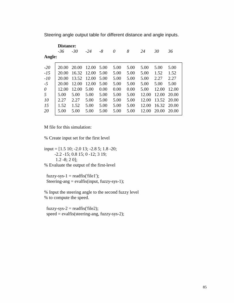
85
Steering angle output table for different distance and angle inputs.
Distance:-36 -30 -24 -8 0 8 24 30 36
Angle:
-20 20.00 20.00 12.00 5.00 5.00 5.00 5.00 5.00 5.00-15 20.00 16.32 12.00 5.00 5.00 5.00 5.00 1.52 1.52-10 20.00 13.52 12.00 5.00 5.00 5.00 5.00 2.27 2.27-5 20.00 12.00 12.00 5.00 5.00 5.00 5.00 5.00 5.000 12.00 12.00 5.00 0.00 0.00 0.00 5.00 12.00 12.005 5.00 5.00 5.00 5.00 5.00 5.00 12.00 12.00 20.0010 2.27 2.27 5.00 5.00 5.00 5.00 12.00 13.52 20.0015 1.52 1.52 5.00 5.00 5.00 5.00 12.00 16.32 20.0020 5.00 5.00 5.00 5.00 5.00 5.00 12.00 20.00 20.00
M file for this simulation:
% Create input set for the first level
input = [1.5 10; -2.0 13; -2.8 5; 1.8 -20; -2.2 -15; 0.8 15; 0 -12; 3 19; 1.2 -8; 2 0];% Evaluate the output of the first-level
fuzzy-sys-1 = readfis('file1'); Steering-ang = evalfis(input, fuzzy-sys-1);
% Input the steering angle to the second fuzzy level% to compute the speed.
fuzzy-sys-2 = readfis('file2); speed = evalfis(steering-ang, fuzzy-sys-2);
86
Fuzzy Associated Memories
Multivalued fuzzy sets can be represented as points in a unit hypercube.
In = [0,1]n
These cubes can be used as a measure of how much one fuzzy set is a subset of
any other fuzzy set. These fuzzy cubes can be mapped. This level of abstraction
provides a surprising and fruitful alternative to the proportional and predicate calculus
reasoning techniques used in the artificial-intelligence expert systems.
The simplest FAM encodes the FAM rule or association (Ai,Bi), which
associates a p - dimensional fuzzy set Bi with the n - dimensional fuzzy set Ai. These
minimal FAMs essentially map one ball in In with one ball in Ip.
A general FAM system:
F: In -> Ip
A FAM system encodes and process in parallel a FAM bank of m rules
(A1,B1)(A2,B2)....(Am,Bm). Each input A to the FAM system activates each stored FAM
rule to different degree.
FAM rules can be represent compound linguistic conditionals. For example
(A1,A2;B) means in linguistic terms as
“IF X 1 is A1 and X2 is A2 THEN Y is B”.
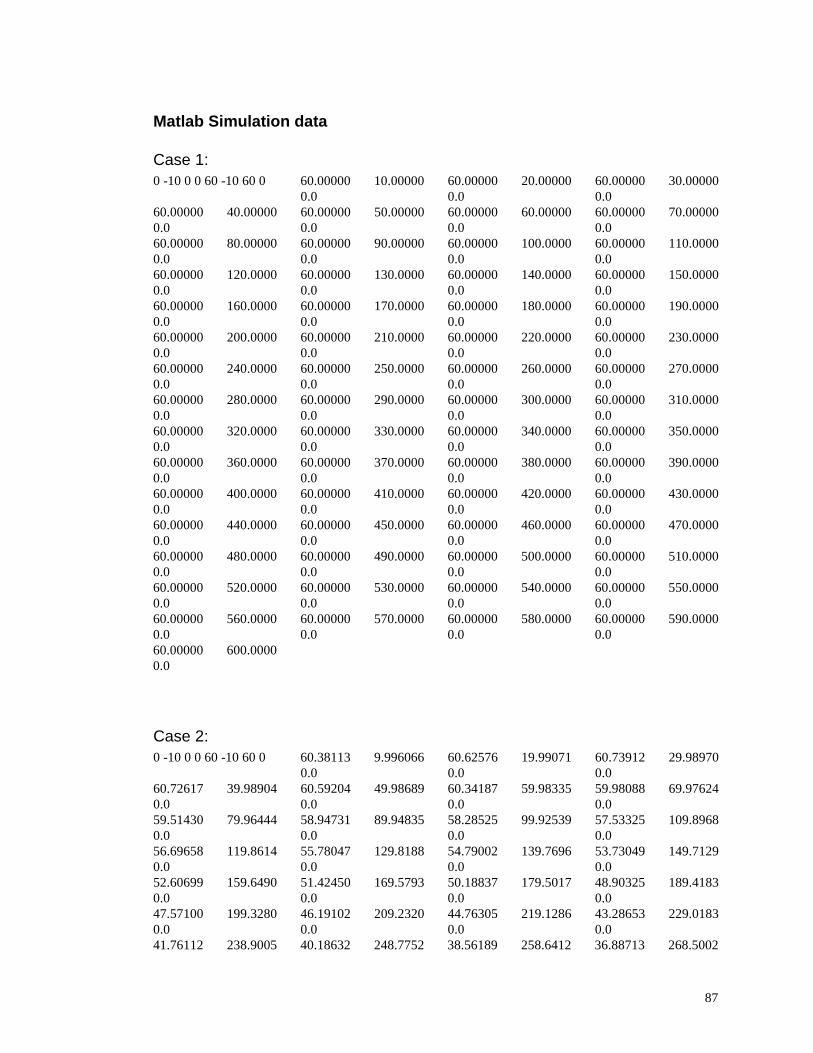
87
Matlab Simulation data
Case 1:0 -10 0 0 60 -10 60 0 60.00000 10.00000
0.060.00000 20.000000.0
60.00000 30.000000.0
60.00000 40.000000.0
60.00000 50.000000.0
60.00000 60.000000.0
60.00000 70.000000.0
60.00000 80.000000.0
60.00000 90.000000.0
60.00000 100.00000.0
60.00000 110.00000.0
60.00000 120.00000.0
60.00000 130.00000.0
60.00000 140.00000.0
60.00000 150.00000.0
60.00000 160.00000.0
60.00000 170.00000.0
60.00000 180.00000.0
60.00000 190.00000.0
60.00000 200.00000.0
60.00000 210.00000.0
60.00000 220.00000.0
60.00000 230.00000.0
60.00000 240.00000.0
60.00000 250.00000.0
60.00000 260.00000.0
60.00000 270.00000.0
60.00000 280.00000.0
60.00000 290.00000.0
60.00000 300.00000.0
60.00000 310.00000.0
60.00000 320.00000.0
60.00000 330.00000.0
60.00000 340.00000.0
60.00000 350.00000.0
60.00000 360.00000.0
60.00000 370.00000.0
60.00000 380.00000.0
60.00000 390.00000.0
60.00000 400.00000.0
60.00000 410.00000.0
60.00000 420.00000.0
60.00000 430.00000.0
60.00000 440.00000.0
60.00000 450.00000.0
60.00000 460.00000.0
60.00000 470.00000.0
60.00000 480.00000.0
60.00000 490.00000.0
60.00000 500.00000.0
60.00000 510.00000.0
60.00000 520.00000.0
60.00000 530.00000.0
60.00000 540.00000.0
60.00000 550.00000.0
60.00000 560.00000.0
60.00000 570.00000.0
60.00000 580.00000.0
60.00000 590.00000.0
60.00000 600.00000.0
Case 2:0 -10 0 0 60 -10 60 0 60.38113 9.996066
0.060.62576 19.990710.0
60.73912 29.989700.0
60.72617 39.989040.0
60.59204 49.986890.0
60.34187 59.983350.0
59.98088 69.976240.0
59.51430 79.964440.0
58.94731 89.948350.0
58.28525 99.925390.0
57.53325 109.89680.0
56.69658 119.86140.0
55.78047 129.81880.0
54.79002 139.76960.0
53.73049 149.71290.0
52.60699 159.64900.0
51.42450 169.57930.0
50.18837 179.50170.0
48.90325 189.41830.0
47.57100 199.32800.0
46.19102 209.23200.0
44.76305 219.12860.0
43.28653 229.01830.0
41.76112 238.9005 40.18632 248.7752 38.56189 258.6412 36.88713 268.5002
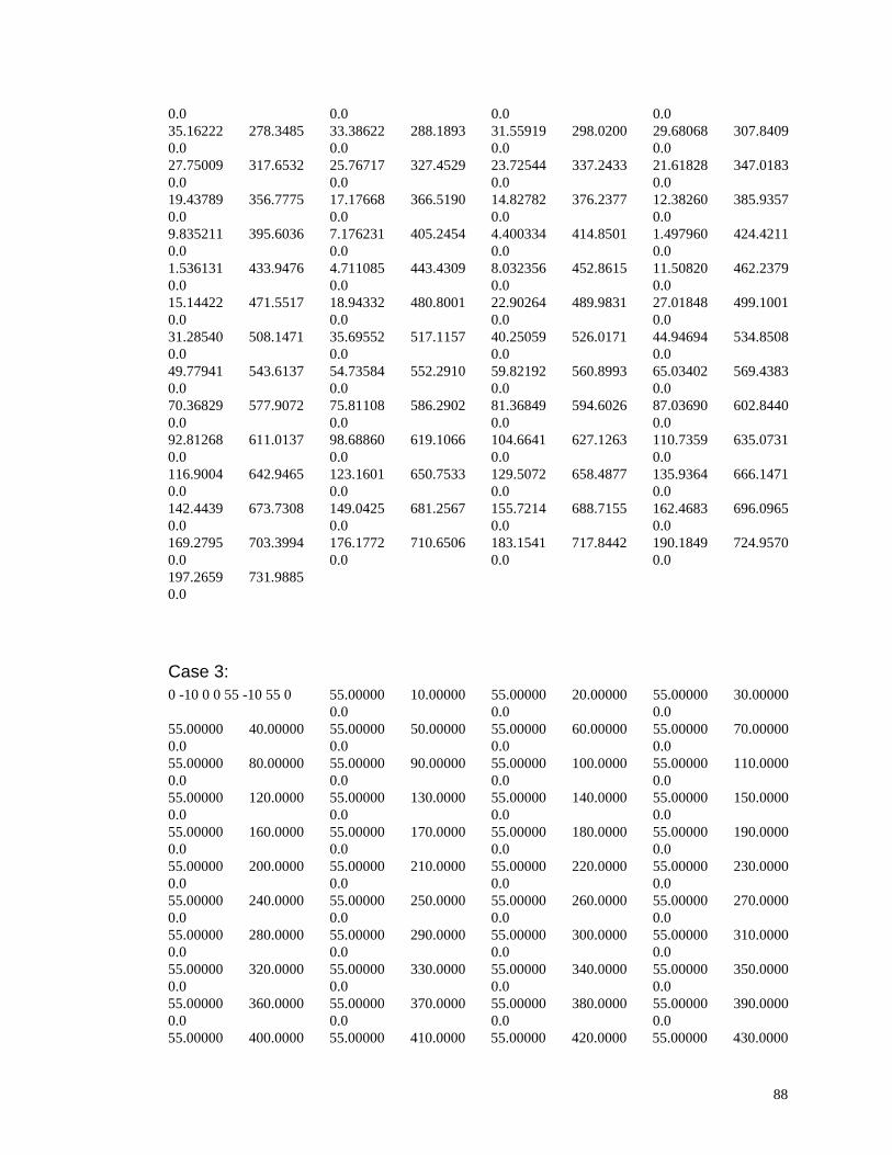
88
0.0 0.0 0.0 0.035.16222 278.34850.0
33.38622 288.18930.0
31.55919 298.02000.0
29.68068 307.84090.0
27.75009 317.65320.0
25.76717 327.45290.0
23.72544 337.24330.0
21.61828 347.01830.0
19.43789 356.77750.0
17.17668 366.51900.0
14.82782 376.23770.0
12.38260 385.93570.0
9.835211 395.60360.0
7.176231 405.24540.0
4.400334 414.85010.0
1.497960 424.42110.0
1.536131 433.94760.0
4.711085 443.43090.0
8.032356 452.86150.0
11.50820 462.23790.0
15.14422 471.55170.0
18.94332 480.80010.0
22.90264 489.98310.0
27.01848 499.10010.0
31.28540 508.14710.0
35.69552 517.11570.0
40.25059 526.01710.0
44.94694 534.85080.0
49.77941 543.61370.0
54.73584 552.29100.0
59.82192 560.89930.0
65.03402 569.43830.0
70.36829 577.90720.0
75.81108 586.29020.0
81.36849 594.60260.0
87.03690 602.84400.0
92.81268 611.01370.0
98.68860 619.10660.0
104.6641 627.12630.0
110.7359 635.07310.0
116.9004 642.94650.0
123.1601 650.75330.0
129.5072 658.48770.0
135.9364 666.14710.0
142.4439 673.73080.0
149.0425 681.25670.0
155.7214 688.71550.0
162.4683 696.09650.0
169.2795 703.39940.0
176.1772 710.65060.0
183.1541 717.84420.0
190.1849 724.95700.0
197.2659 731.98850.0
Case 3:0 -10 0 0 55 -10 55 0 55.00000 10.00000
0.055.00000 20.000000.0
55.00000 30.000000.0
55.00000 40.000000.0
55.00000 50.000000.0
55.00000 60.000000.0
55.00000 70.000000.0
55.00000 80.000000.0
55.00000 90.000000.0
55.00000 100.00000.0
55.00000 110.00000.0
55.00000 120.00000.0
55.00000 130.00000.0
55.00000 140.00000.0
55.00000 150.00000.0
55.00000 160.00000.0
55.00000 170.00000.0
55.00000 180.00000.0
55.00000 190.00000.0
55.00000 200.00000.0
55.00000 210.00000.0
55.00000 220.00000.0
55.00000 230.00000.0
55.00000 240.00000.0
55.00000 250.00000.0
55.00000 260.00000.0
55.00000 270.00000.0
55.00000 280.00000.0
55.00000 290.00000.0
55.00000 300.00000.0
55.00000 310.00000.0
55.00000 320.00000.0
55.00000 330.00000.0
55.00000 340.00000.0
55.00000 350.00000.0
55.00000 360.00000.0
55.00000 370.00000.0
55.00000 380.00000.0
55.00000 390.00000.0
55.00000 400.0000 55.00000 410.0000 55.00000 420.0000 55.00000 430.0000
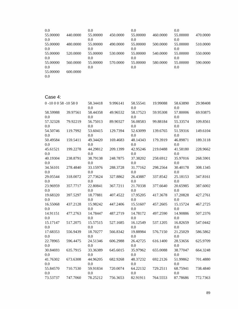
89
0.0 0.0 0.0 0.055.00000 440.00000.0
55.00000 450.00000.0
55.00000 460.00000.0
55.00000 470.00000.0
55.00000 480.00000.0
55.00000 490.00000.0
55.00000 500.00000.0
55.00000 510.00000.0
55.00000 520.00000.0
55.00000 530.00000.0
55.00000 540.00000.0
55.00000 550.00000.0
55.00000 560.00000.0
55.00000 570.00000.0
55.00000 580.00000.0
55.00000 590.00000.0
55.00000 600.00000.0
Case 4:0 -10 0 0 58 -10 58 0 58.34418 9.996141
0.058.55541 19.990880.0
58.63890 29.984080.0
58.59988 39.975610.0
58.44358 49.965320.0
58.17523 59.953080.0
57.80006 69.938750.0
57.32328 79.922190.0
56.75013 89.903270.0
56.08583 99.881840.0
55.33574 109.85610.0
54.50746 119.79920.0
53.60415 129.73940.0
52.63099 139.67650.0
51.59316 149.61040.0
50.49584 159.54110.0
49.34420 169.46830.0
48.14343 179.39190.0
46.89871 189.31180.0
45.61521 199.22780.0
44.29812 209.13990.0
42.95246 219.04880.0
41.58180 228.96620.0
40.19304 238.87910.0
38.79138 248.78750.0
37.38202 258.69120.0
35.97016 268.59010.0
34.56101 278.48400.0
33.15976 288.37280.0
31.77162 298.25640.0
30.40178 308.13450.0
29.05544 318.00720.0
27.73624 327.88620.0
26.43887 337.85420.0
25.18153 347.81610.0
23.96959 357.77170.0
22.80841 367.72110.0
21.70338 377.66400.0
20.65985 387.60020.0
19.68320 397.52970.0
18.77881 407.45220.0
17.95205 417.36780.0
17.20828 427.27610.0
16.55068 437.21280.0
15.98242 447.24060.0
15.51607 457.26050.0
15.15724 467.27250.0
14.91151 477.27630.0
14.78447 487.27190.0
14.78172 497.25900.0
14.90886 507.23760.0
15.17147 517.20750.0
15.57515 527.16850.0
16.12549 537.12050.0
16.82659 547.04420.0
17.68353 556.94390.0
18.70277 566.83420.0
19.88984 576.71500.0
21.25029 586.58620.0
22.78965 596.44750.0
24.51346 606.29880.0
26.42725 616.14000.0
28.53656 625.97090.0
30.84693 635.79150.0
33.36389 645.60150.0
35.97962 655.00880.0
38.77047 664.32480.0
41.76302 673.63080.0
44.96205 682.92680.0
48.37232 692.21260.0
51.99862 701.48800.0
55.84570 710.75300.0
59.91834 720.00740.0
64.22132 729.25110.0
68.75941 738.48400.0
73.53737 747.7060 78.25212 756.3653 82.91911 764.5553 87.78686 772.7363
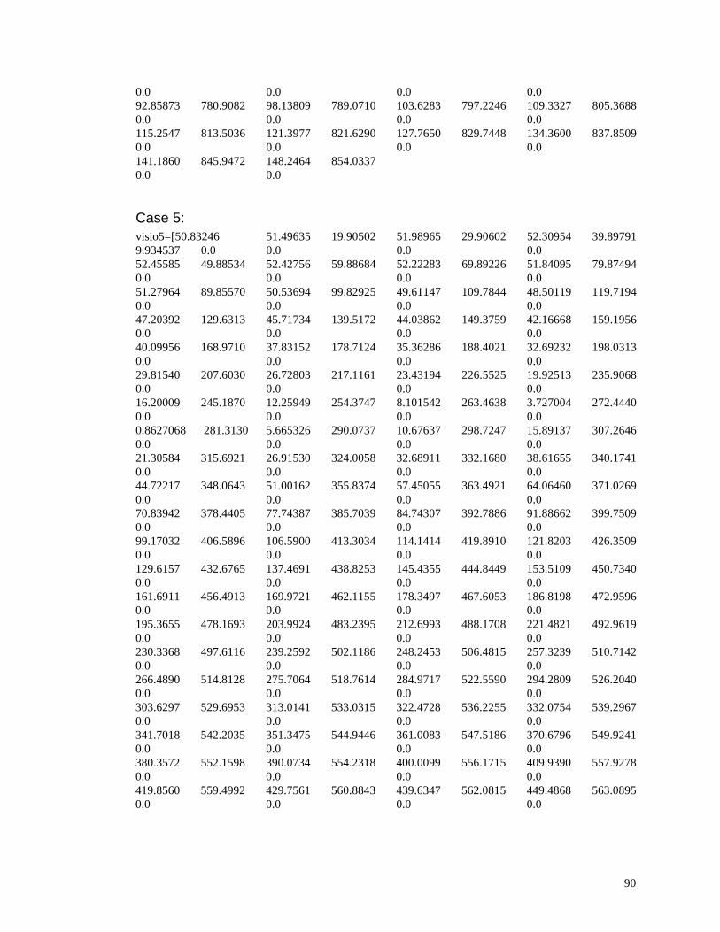
90
0.0 0.0 0.0 0.092.85873 780.90820.0
98.13809 789.07100.0
103.6283 797.22460.0
109.3327 805.36880.0
115.2547 813.50360.0
121.3977 821.62900.0
127.7650 829.74480.0
134.3600 837.85090.0
141.1860 845.94720.0
148.2464 854.03370.0
Case 5:visio5=[50.832469.934537 0.0
51.49635 19.905020.0
51.98965 29.906020.0
52.30954 39.897910.0
52.45585 49.885340.0
52.42756 59.886840.0
52.22283 69.892260.0
51.84095 79.874940.0
51.27964 89.855700.0
50.53694 99.829250.0
49.61147 109.78440.0
48.50119 119.71940.0
47.20392 129.63130.0
45.71734 139.51720.0
44.03862 149.37590.0
42.16668 159.19560.0
40.09956 168.97100.0
37.83152 178.71240.0
35.36286 188.40210.0
32.69232 198.03130.0
29.81540 207.60300.0
26.72803 217.11610.0
23.43194 226.55250.0
19.92513 235.90680.0
16.20009 245.18700.0
12.25949 254.37470.0
8.101542 263.46380.0
3.727004 272.44400.0
0.8627068 281.31300.0
5.665326 290.07370.0
10.67637 298.72470.0
15.89137 307.26460.0
21.30584 315.69210.0
26.91530 324.00580.0
32.68911 332.16800.0
38.61655 340.17410.0
44.72217 348.06430.0
51.00162 355.83740.0
57.45055 363.49210.0
64.06460 371.02690.0
70.83942 378.44050.0
77.74387 385.70390.0
84.74307 392.78860.0
91.88662 399.75090.0
99.17032 406.58960.0
106.5900 413.30340.0
114.1414 419.89100.0
121.8203 426.35090.0
129.6157 432.67650.0
137.4691 438.82530.0
145.4355 444.84490.0
153.5109 450.73400.0
161.6911 456.49130.0
169.9721 462.11550.0
178.3497 467.60530.0
186.8198 472.95960.0
195.3655 478.16930.0
203.9924 483.23950.0
212.6993 488.17080.0
221.4821 492.96190.0
230.3368 497.61160.0
239.2592 502.11860.0
248.2453 506.48150.0
257.3239 510.71420.0
266.4890 514.81280.0
275.7064 518.76140.0
284.9717 522.55900.0
294.2809 526.20400.0
303.6297 529.69530.0
313.0141 533.03150.0
322.4728 536.22550.0
332.0754 539.29670.0
341.7018 542.20350.0
351.3475 544.94460.0
361.0083 547.51860.0
370.6796 549.92410.0
380.3572 552.15980.0
390.0734 554.23180.0
400.0099 556.17150.0
409.9390 557.92780.0
419.8560 559.49920.0
429.7561 560.88430.0
439.6347 562.08150.0
449.4868 563.08950.0