Embed Size (px)
Citation preview

Brazilian Journal of Physics
ISSN: 0103-9733
Sociedade Brasileira de Física
Brasil
Rodrigues, Clóves G.; Vasconcellos, Áurea R.; Galvão Ramos, J.; Luzzi, Roberto
Response Function Theory for Many-Body Systems Away from Equilibrium: Conditions of Ultrafast-
Time and Ultrasmall-Space Experimental Resolution
Brazilian Journal of Physics, vol. 45, núm. 1, 2015, pp. 166-193
Sociedade Brasileira de Física
Sâo Paulo, Brasil
Available in: http://www.redalyc.org/articulo.oa?id=46433753021
How to cite
Complete issue
More information about this article
Journal's homepage in redalyc.org
Scientific Information System
Network of Scientific Journals from Latin America, the Caribbean, Spain and Portugal
Non-profit academic project, developed under the open access initiative
Braz J Phys (2015) 45:166–193DOI 10.1007/s13538-014-0280-0
CONDENSED MATTER
Response Function Theory for Many-Body SystemsAway from Equilibrium: Conditions of Ultrafast-Timeand Ultrasmall-Space Experimental Resolution
Cloves G. Rodrigues · Aurea R. Vasconcellos ·J. Galvao Ramos · Roberto Luzzi
Received: 10 October 2013 / Published online: 19 November 2014© Sociedade Brasileira de Fısica 2014
Abstract A response function theory and scattering theoryapplicable to the study of physical properties of systemsdriven arbitrarily far removed from equilibrium, special-ized for dealing with ultrafast processes, and in conditionsof space resolution (including the nanometric scale) arepresented. The derivation is done in the framework ofa Gibbs-style nonequilibrium statistical ensemble formal-ism. The observable properties are shown to be connectedwith time- and space-dependent correlation functions out ofequilibrium. A generalized fluctuation-dissipation theorem,which relates these correlation functions with generalizedsusceptibilities, is derived. The method of nonequilibrium-thermodynamic Green functions, which proves useful forcalculations, is also presented. Two illustrative applicationsof the formalism, which study optical responses in ultra-fast laser spectroscopy and Raman scattering of electrons inIII-N semiconductors (of “blue diodes”) driven away fromequilibrium by electric fields of moderate to high intensities,are described.
Keywords Semiconductors · Response function ·Scattering theory · Ultrafast processes
C. G. Rodrigues (�)Departamento de Fısica, Pontifıcia Universidade Catolicade Goias, Goiania, Goias 74605-010, Brazile-mail: [email protected]
A. R. Vasconcellos · J. G. Ramos · R. LuzziCondensed Matter Physics Department, Institute of Physics“Gleb Wataghin”, State University of Campinas-Unicamp,Campinas, SP 13083-859, Brazil
R. LuzziURL www.ifi.unicamp.br/∼aurea
1 Introduction
The renowned Ryogo Kubo once stated that “statisticalmechanics has been considered a theoretical endeavor.However, statistical mechanics exists for the sake of the realworld, not for fictions. Further progress can only be hopedby closed cooperation with experiment” [1]. This is nowa-days particularly relevant because the notable developmentof all modern technology, fundamental for the progress andwell being of the world society, poses a great deal of stressin the realm of basic physics, more precisely on thermo-statistics. Thus, on the one hand, we face situations inelectronics and optoelectronics involving physical-chemicalsystems far removed from equilibrium, where ultrafast(pico- and femtosecond scale) and nonlinear processes arepresent. Further, we need to be aware of the rapid unfoldingof nano-technologies and use of low-dimensional systems(e.g., nanometric quantum wells and quantum dots in semi-conductors heterostructures) [2]. Altogether, this demandsaccess to a statistical mechanics capable of efficiently deal-ing with such requirements. On the other hand, one needsto face the study of soft matter and fluids with complexstructures (usually of the average self-affine fractal-liketype) [3]. This is relevant for technological improvement inindustries like, for example, those of polymers, petroleum,cosmetics, food, electronics, and photonics (conductingpolymers and glasses), in medical engineering, etc. More-over, in both types of the above-mentioned situations, thereoften appear difficulties of description and objectivity (exis-tence of so-called hidden constraints), which impair theproper application of the conventional ensemble approachused in the general, logically and physically sound, andwell-established Boltzmann-Gibbs statistics. An attempt topartially overcome such difficulties calls for unconventionalapproaches [4–7].
Braz J Phys (2015) 45:166–193 167
As already pointed out, a central objective of anynonequilibrium statistical theory is to provide an under-standing of the physics underlying relaxation phenomenathat can be evidenced in experiments. The statistical theorymust therefore be coupled with a response function theory.This is the subject of this paper. Specifically, we deal withthe nonequilibrium statistical ensemble formalism (NESEFfor short) [8–13].
Nowadays, two approaches appear to be the most favor-able to deal with systems within an ample scope of nonequi-librium conditions. On the one hand, we have numericalsimulation methods [14], also referred to as computationalphysics. In particular, to this branch belongs the nonequi-librium molecular-dynamics (NMD) [15], a computationalmethod created for modeling physical systems at the micro-scopic level that proves adequate to study the molecularbehavior of several physical processes. On the other hand,we have the kinetic theory based on the far-reaching gen-eralization of Gibbs’ ensemble formalism, NESEF [12, 13,16]. NESEF is a powerful formalism that provides an ele-gant, practical, and physically clear picture for describingirreversible processes. It is adequate to deal with a largeclass of experimental situations, as for example, semicon-ductors far from equilibrium, and offers good agreementwith other theoretical work and with experimental results[17–35].
Early work in computational physics laid the founda-tions of modern Monte Carlo simulations—the name thathighlights the importance of random numbers in the proce-dure. After the initial groundwork in the early 1970s, com-puter simulation developed rapidly, in pace with the rapiddevelopment of computer hardware. Computer-simulationtechniques have benefited from the introduction of sub-stantially improved methods to measure transport coeffi-cients, the development of stochastic dynamics methods,and other advances. How do the more sophisticated ver-sions of computational modeling compare with the kineticequation approaches (such as those based on NESEF, andit can be noticed that here, computers play an incidental,calculational part)?
Apparently, they are approximately equivalent (in thesense of similar numerical results and in good comparisonwith experimental results) when dealing with many-bodysystems not displaying higher-order correlations and vari-ances, a situation that may arise in analyses of liquidspresenting hydrodynamics and nonlinear instabilities. In thecase of semiconductors well described by single elementaryexcitations (phonons, Landau-Bloch band electrons, exci-tons, magnons, polaritons, etc.), both approaches seem toproduce comparable optical and transport properties. Asan example, consider the mobility in n-doped polar semi-conductors [34, 35]: in several cases, involving GaN andGaAs under intermediate to high electric fields, very good
agreement was found between the two procedures and withthe available experimental results. Although one particularcase showed no agreement, the results from the kinetic the-ory curiously came closer to experiment than those from theMonte Carlo calculations. We conjecture that the presenceof certain “hidden constants” leads to this state of affairs.
The present structure of the NESEF formalism consistsof an extension and generalization of earlier pioneeringapproaches, among which we can pinpoint the works ofKirkwood [36], Green [37], Mori-Oppenheim-Ross [38],Mori [39], and Zwanzig [40]. NESEF has been approachedfrom different points of view: some are based on heuris-tic arguments, others on projection-operator techniques, theformer following Kirkwood and Green, the latter followingZwanzig and Mori.
The formalism has been systematized and largelyimproved by the Russian School of Statistical Physics,which can be considered to have been started by therenowned Nicolai Nicolaievich Bogoliubov (e.g., see Ref.[41]). We may also recall the ideas of Nicolai SergeievichKrylov [42] and more recently mainly through the relevantcontributions of Dimitrii Zubarev [8, 9], Sergei Peletmin-skii [43], and others. We have presented in Refs. [12, 13]a systematization, as well as generalizations and conceptualdiscussions, of the matter.
These distinct approaches to NESEF can be broughttogether under a unique variational principle. This was orig-inally done by Zubarev and Kalashnikov [44] and laterreconsidered in Refs. [9, 12, 13]. It consists of maximizing,in the context of information theory, the Gibbs statisticalentropy, that is, the average of the negative logarithm ofthe statistical distribution function [45, 46], which in com-munication theory is the Shannon informational entropy[47, 48], subject to certain constraints and including spatialnonlocality, retro-effects, and irreversibility at the macro-scopic level.
Concerning response function theory, the usual approachto calculating linear responses to mechanical perturba-tions (e.g., Refs. [49–54]) relies on expansions in terms ofequilibrium correlation functions. The initial condition isdefined by the equilibrium with a thermal reservoir, and theevolution of the system then studied as if it were isolatedfrom all external influences except the driving field. Let ushere consider a mechanical perturbation applied to a sys-tem that is already far from equilibrium, in which systemirreversible processes are unfolding that can be describedby evolution equations for a basic set of macrovariables inthe nonequilibrium-thermodynamic space of states. SinceNESEF provides a seemingly powerful method to describethe macrostate of this system, it is appealing to derivea response function theory based on correlation functionsin the unperturbed nonequilibrium state of the system.Schemes of this type have been proposed [52–54], and we

168 Braz J Phys (2015) 45:166–193
next systematize and extend this treatment to allow thetreatment of experiments involving time resolution (includ-ing the ultrafast time scale of pico- and femtoseconds) andspace resolution (including those in the bourgeoning fieldsof nanoscience and nanotechnology).
We will show the connection between the observableproperties and out-of-equilibrium correlation functions;derive a generalized fluctuation-dissipation theorem, relat-ing correlation functions and generalized susceptibilities;and present a method useful to calculate nonequilibrium-thermodynamic Green functions. This is done in Sections 2,3, and 4. In Section 5, we present a scattering theory, underthe same conditions, namely including time and space res-olution, for far-from equilibrium systems. The connectionbetween the scattering theory and response function theoryfollows from application of the nonequilibrium fluctuation-dissipation theorem.
Finally, in Section 6, we present a couple of illustra-tions showing the theory at work in the study of two kindof experiments, namely optical responses in ultrafast laserspectroscopy of polar semiconductors and Raman scatteringof electrons in doped III-N semiconductors (“blue diodes”)in the presence of electric fields with moderate to highintensities. In the latter case, the nonequilibrium fluctuation-dissipation theorem connects the Raman spectrum with non-linear transport properties (nonlinear and time-dependentconductivity and diffusion coefficient, and a generalized—nonlinear and time-dependent—Einstein-relation).
2 Response Function Theory for Far-from-EquilibriumSystems
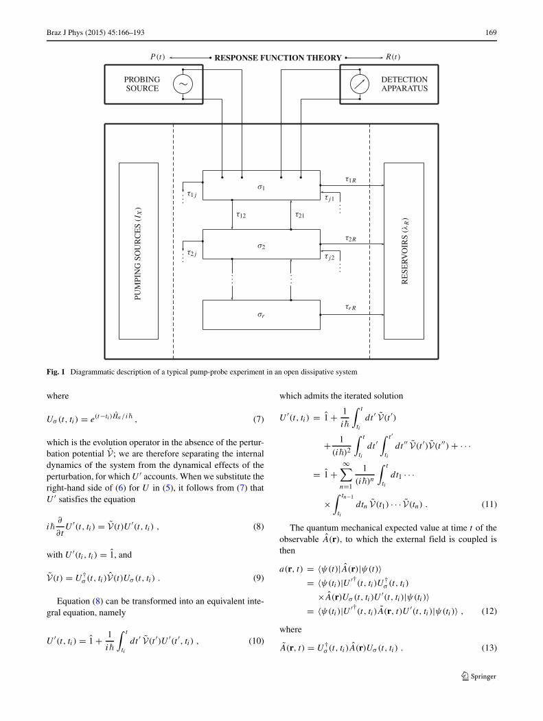
We consider an open many-body system out of equilibriumin contact with a set of reservoirs and under the action ofpumping sources. We are essentially presenting the mostgeneral experiment one can think of, namely a sample (theopen system of interest, which comprises very many degreesof freedom) subject to given experimental conditions, asdiagrammatically described by Fig. 1.
The sample in Fig. 1 is constituted of a number of sub-systems, σj , (or better to say, subdegrees of freedom; forexample, in a solid-state matter, those associated with elec-trons, lattice vibrations, excitons, impurity states, collectiveexcitations as plasmons, magnons, etc., hybrid excitations aspolarons, polaritons, plasmaritons, and so on). They interactamong themselves via interaction potentials responsible forenergy and momentum exchange at certain rates τij . Pump-ing sources act on different subsystems of the sample—viaparticular types of fields, electric, magnetic, electromag-netic, etc.—well characterized when the experiment is setup. The energy in excess of equilibrium received by thesystem is relaxed to the external reservoirs τjR . Finally,
the experiment is carried out: an external probing source,represented in the figure by P(t), is coupled to one ormore sample subsystems, and a certain response, say R(t),is detected by a measuring apparatus (e.g., an ammeter, aspectrometer, etc.).
The pumping sources exert their influence on the opensystem through the fields they generate, say the magnetic,electric, or electromagnetic fields generated, for example,by a laser. In scattering experiments, the agent is the inter-action potential with the particles of an incoming beam.
Let the Hamiltonian describing the system under theaction of the pumping-source fields that drive it away fromequilibrium plus the interactions with the reservoirs andfields be Hσ . The total Hamiltonian is, then,
H (t) = Hσ + V(t) , (1)
where V(t) describes the coupling to the external perturbingapparatus. For the latter, we adopt the form
V(t) = −∫
d3r ′ F(r′, t)A(r′) . (2)
Here, F is the perturbing force, F = −δV/δA(r′), whereδ is a functional derivative, and A(r′) is the system observ-able to which the perturbation is coupled. We recall that thesystem is in contact with ideal reservoirs.
We take the statistical operator to be the product ofthe one of the system �ε(t) by the stationary canoni-cal distribution of the reservoirs �R, denoted by the formRε(t) = �ε(t) × �R [12, 13] (see Appendix). Moreover,Hσ = H0 + H1 + W = H0 + H ′, with the definitionH ′ ≡ H1 + W , where H1 accounts for all the interac-tions within the system and W for the interaction withthe surroundings. The Hamiltonian H0 describes the freeelementary excitations.
The Schrodinger equation then reads
i�∂
∂t|ψ(t)〉 = H (t)|ψ(t)〉 . (3)
Given the initial condition |ψ(ti)〉 at time ti when theperturbation is switched on, the formal solution of (3) is
|ψ(t)〉 = U(t, ti)|ψ(ti)〉 , (4)
where U is the evolution operator satisfying that
i�∂
∂tU(t, ti ) = H (t)U(t, ti ) , (5)
where U(ti , ti) = 1 (the unit operator), which we recall, isunitary, that is U†U = 1.
We now introduce the interaction representation, definedby the expression
U(t, ti ) = Uσ (t, ti)U′(t, ti) , (6)
Braz J Phys (2015) 45:166–193 169
Fig. 1 Diagrammatic description of a typical pump-probe experiment in an open dissipative system
where
Uσ (t, ti) = e(t−ti)Hσ /i� , (7)
which is the evolution operator in the absence of the pertur-bation potential V ; we are therefore separating the internaldynamics of the system from the dynamical effects of theperturbation, for which U ′ accounts. When we substitute theright-hand side of (6) for U in (5), it follows from (7) thatU ′ satisfies the equation
i�∂
∂tU ′(t, ti) = V(t)U ′(t, ti) , (8)
with U ′(ti, ti ) = 1, and
V(t) = U†σ (t, ti)V(t)Uσ (t, ti) . (9)
Equation (8) can be transformed into an equivalent inte-gral equation, namely
U ′(t, ti) = 1 + 1
i�
∫ t
ti
dt ′ V(t ′)U ′(t ′, ti) , (10)
which admits the iterated solution
U ′(t, ti) = 1 + 1
i�
∫ t
ti
dt ′ V(t ′)
+ 1
(i�)2
∫ t
ti
dt ′∫ t ′
ti
dt ′′ V(t ′)V(t ′′) + · · ·
= 1 +∞∑
n=1
1
(i�)n
∫ t
ti
dt1 · · ·
×∫ tn−1
ti
dtn V(t1) · · · V(tn) . (11)
The quantum mechanical expected value at time t of theobservable A(r), to which the external field is coupled isthen
a(r, t) = 〈ψ(t)|A(r)|ψ(t)〉= 〈ψ(ti)|U ′†(t, ti)U
†σ (t, ti)
×A(r)Uσ (t, ti)U′(t, ti)|ψ(ti)〉
= 〈ψ(ti)|U ′†(t, ti)A(r, t)U ′(t, ti)|ψ(ti)〉 , (12)
where
A(r, t) = U†σ (t, ti)A(r)Uσ (t, ti) . (13)
170 Braz J Phys (2015) 45:166–193
According to (11), we have that
a(r, t) = 〈ψ(ti)|(
1 − 1
i�
∫ t
ti
dt ′ V(t ′) + · · ·)
×A(r, t)
(1 + 1
i�
∫ t
ti
dt ′ V(t ′) + · · ·)
|ψ(ti)〉,(14)
where we have used that V is Hermitian.Let the system be far from equilibrium at the initial time
ti , when perturbation V(t) is applied, and let the perturba-tion be weak. We can then truncate the expansion in (14)to first order in V, that is, consider from now on a linearresponse theory, to obtain that
a(r, t) = a(r, ti)+ 1
i�
∫ t
ti
dt ′ 〈ψ(ti)|[A(r, t), V(t ′)]|ψ(ti)〉 ,
(15)
where
a(r, ti) = 〈ψ(ti)|A(r)|ψ(ti)〉 (16)
is the expectation value for the observable at the time ti ,prior to the application of the perturbation.
From (2), we have that
a(r, t) = − 1
i�
∫ t
ti
dt ′∫
d3r ′〈ψ(ti)|[A(r, t), A(r′, t ′)]× F(r′, t ′)|ψ(ti)〉, (17)
where a(r, t) = a(r, t) − a(r, ti) is the departure of theobservable A from its value at the initial time under theaction of the perturbing potential.
Introducing the statistical operator for the pure (quantummechanical) state, namely
P(ti) = |ψ(ti)〉〈ψ(ti)| , (18)
which, we recall, is a projection operator over the vectorstate |ψ(ti)〉, we can rewrite (17) in the form
a(r, t) = − 1
i�
∫ t
−∞dt ′
∫d3r ′Tr{[A(r, t), A(r′, t ′)]P(ti)}
×F(r′, t ′), (19)
where we have let ti → −∞ and adiabatically applied theperturbation.
To examine the macroscopic state, we next average (19)over the nonequilibrium ensemble of pure states, com-patible with the macroscopic conditions under which thesample is prepared. If as usual we call Pn(ti ) the statis-tical operator for the pure state in, say, the n-th replica,and pn the probability of such replica in the correspondingGibbs ensemble, the statistical average over the ensembleof mixed states of the system and over the states of the
reservoir (which is coupled to the system by the interactionW ) is
〈A(r)|t〉 = − 1
i�
∫ t
−∞dt ′
∫d3r ′ ∑
n
pnTr
×{[A(r, t), A(r′, t ′)]Pn(ti ) × �R
}F(r′, t ′)
= − 1
i�
∫ t
−∞dt ′
∫d3r ′Tr
×{[A(r, t), A(r′, t ′)]�ε(ti )�R}F(r′, t ′) , (20)
with
�ε(ti ) =∑n
pnPn(ti ) =∑n
pn|ψn(ti )〉〈ψn(ti)| , (21)
On the left-hand side of (20), we have introduced thenotation
〈A(r)|t〉 = Tr{A(r)Rε(t)} − Tr{A(r)Rε(ti )}, (22)
where, we recall, Rε(t) = �ε(t) × �R.Equation (20) can be rewritten in the form
〈A(r)|t〉 = − 1
i�
∫ t
−∞dt ′
∫d3rTr
×{[A(r), A(r′, t ′ − t)]Rε(t)
}F(r′, t ′) (23)
since
Tr{[U†σ (t, ti)A(r)Uσ (t, ti), U†
σ (t ′, ti)A(r′)Uσ (t ′, ti)]Rε(ti )}= Tr{A(r), A(r′, t ′ − t)Rε(t)}, (24)
where we have used the invariance of the trace operation bycyclical permutations and the group properties of operatorsU .
Under nonequilibrium conditions, the system is notinvariant under time translations, since a statistical opera-tor describing the irreversible evolution of the macroscopicstate is time dependent; the operator A(t ′ − t) in (24) showstime-translational invariance, because the time dependencestems from the microdynamical evolution governed byHamiltonian Hσ . Moreover, introducing the definitions
χ ′′(r, r′; t ′− t|t) = 1
2�Tr{[A(r), A(r′, t ′ − t)]Rε(t)} , (25)
χ(r, r′; t − t ′|t) = 2i�(t − t ′)χ ′′(r, r′; t ′ − t|t) , (26)
where � denotes Heaviside’s step function, we see that (20)reduces to the expression
〈A(r)|t〉 =∫ ∞
−∞dt ′
∫d3r ′ χ(r, r′; t − t ′|t)F(r′, t ′) .
(27)

Braz J Phys (2015) 45:166–193 171
Taking advantage of the integral representation of Heav-iside’s step function, namely
�(τ) = lims→+0
i
∫ ∞
−∞dω
2π
e−iωτ
(ω + is), (28)
we find, after a few manipulation, that the Fourier trans-form in time τ = t − t ′ of the nonequilibrium generalizedsusceptibility of (26) is given by the equality
χ(r, r′; ω|t) =∫ ∞
−∞dω′
π
χ ′′(r, r′; ω′|t)(ω′ − ω − is)
, (29)
where s → +0, and χ ′′(r, r′; ω′|t) is the Fourier transformat frequency ω of the τ -dependent χ ′′ of (25), namely
χ ′′(r, r′; ω|t) =∫ ∞
−∞dτ χ ′′(r, r′; −τ |t)eiωτ . (30)
Using the identities
lims→+0
1
x ± is= P
{1
x∓ iπδ(x)
}, (31)
which are the so-called advanced and retarded Heisenbergdelta functions, where P stands for the principal value, (29)takes the form
χ(r, r′; ω|t) = Re{χ(r, r′; ω|t)} + iIm{χ(r, r′; ω|t)}= P
{∫ ∞
−∞dω′
π
χ ′′(r, r′; ω′|t)(ω′ − ω)
+iχ ′′(r, r′; ω|t)}
, (32)
where Re and Im stand for the real and imaginary parts,respectively.
We then have that
Im{χ(r, r′; ω|t)} = χ ′′(r, r′; ω|t) , (33)
Re{χ(r, r′; ω|t)} = pv
{∫ ∞
−∞dω′
π
Imχ(r, r′; ω′|t)(ω′ − ω)
},
(34)
after recalling that χ ′′(r, r′; ω|t) is a real quantity [see (51),below].
Equation (34) is one of the so-called generalized Kramer-Kronig relations. The second such generalized relation,
Im{χ(r, r′; ω|t)} = −P{∫ ∞
−∞dω′
π
Re{χ(r, r′; ω′|t)}(ω′ − ω)
},
(35)
can be obtained from (34) and the operational relation
P∫ ∞
−∞dω′′
π(ω−ω′′)−1(ω′′ −ω′)−1 = −πδ(ω−ω′) . (36)
We recall that Kramer-Kronig relations are consequencesof the principle of causality, related to behavior of the sus-ceptibility in the complex plane. More specifically, onceextended to the complex z = ω + iy plane, χ(r, r′; z|t), haspoles in the lower half plane, but is regular in the upper halfplane. Furthermore, Re{χ} is an even function of ω, whileIm{χ} is an odd function. Therefore, as one would expect,χ(r, r′; ω|t) shares the properties of the equilibrium sus-ceptibility, which will be discussed in connection with (52),below.
Moreover, Im{χ(r, r′; ω|t)} is related to the powerabsorbed by the system. To show this, we first notice thatthe time-dependent external force applied on the system,a real quantity, can be Fourier analyzed to yield a linearsuperposition of Fourier components, namely
F(r′, t ′) =∫
dω1
2F(r′, ω)
(eiωt ′ + e−iωt ′
). (37)
Consider, then, the average over time t ′ (and then τ ) ofthe power absorbed by the system in a time interval t (typ-ically the experimental resolution time), which is given bythe expression
W(t)= 1
t
∫ t+t
t
dt ′ dE(t ′)dt ′
= 1
t
∫ t+t
t
dt ′ d
dt ′Tr{H (t ′)Rε(t
′)}
= 1
t
∫ t+t
t
dt ′Tr
{∂H (t ′)
∂t ′Rε(t
′)+H (t ′) ∂
∂t ′Rε(t
′)}
.
(38)
But since
Tr
{H (t ′)
∂
∂t ′Rε(t
′)}
= 1
i�Tr{[H (t ′), H (t ′)]Rε(t
′)}
= 0,
(39)
where we have used that Rε satisfies Liouville equation, wesee that
W(t) = 1
t
∫ t+t
t
dt ′ Tr
{∂H (t ′)
∂t ′Rε(t
′)}
= 1
t
∫ t+t
t
dt ′ Tr
{∂V(t ′)
∂t ′Rε(t
′)}
= − 1
t
∫ t+t
t
dt ′∫
d3r ′Tr{A(r′)Rε(t′)}∂F(r′, t ′)
∂t ′,
(40)
with V given by (2).
172 Braz J Phys (2015) 45:166–193
Account taken that
T r{A(r′)Rε(t)} = T r{A(r′)U(t ′, ti)Rε(ti )U†(t ′, ti)}
= T r{U†(t ′, ti )A(r′)U(t ′, ti)Rε(ti )}= T r{U ′†(t ′, ti)A(r′, t ′)U ′(t ′, ti)Rε(ti )},
(41)
where we have used (6) and (13), with the help of (11) tofirst order, i.e., within linear response, and of (20), we findthat
W(t) = 1
i�t
∫ t+t
t
dt ′∫
d3r ′∫ t ′
−∞dt ′′
∫d3r ′′
Tr{[A(r′, t ′), A(r′′, t ′′)]Rε(ti )}F(r′′, t ′′)∂F(r′, t ′)∂t ′
= − 1
t
∫ t+t
t
dt ′∫
d3r ′A(r′, t ′)∂F(r′, t ′)
∂t ′, (42)
with A defined by (20).In view of (27), we can write (42) in the alternative form
W(t) = − 1
t
∫ t+t
t
dt ′∫
d3r ′∫
d3r ′′∫ ∞
−∞dτ χ
×(r′, r′′; τ |t ′)F(r′′, τ + t ′)∂F(r′, t ′)∂t ′
, (43)
where τ = t ′′ − t ′From (37) and the definition of the Fourier transform of
χ , it follows that
W(t) = − 1
t
∫ t+t
t
dt ′∫
d3r ′∫
d3r ′′∫
dωiωF(r′′, ω)
×F(r′, ω){χ∗(r′, r′′; ω|t ′)(e2iωt ′ − 1)
−χ(r′, r′′; ω|t ′)(e−2iωt ′ − 1)}
. (44)
Consider now a particular situation without ultrafastrelaxation, so that Rε(t
′) varies weakly in the interval t
and is therefore approximately equal to Rε(t). If t islarge in comparison with 2π/ω, the exponentials on theright-hand side of (44) cancel on average, and from (23), itfollows that
W(t)= 1
2
∫d3r ′
∫d3r ′′
∫dωF(r′, ω)F(r′′, ω)α(r′, r′′; ω|t),
(45)
where
α(r′, r′′; ω|t) = ωχ ′′(r′, r′′; ω|t) (46)
can be identified with an absorption coefficient at frequencyω associated to the perturbing force at the macroscopic(nonequilibrium thermodynamic) state of the system attime t .
Evidently, and this is a fundamental point to be stressed,the generalized susceptibility depends on �ε, it is a
functional of the time- (and eventually of the space-)dependent variables that characterized the nonequilibrium-thermodynamic state of the system, then the calculus ofresponses needs be coupled with the one of the equationsof evolution for the basic variables, as given by the non-linear quantum kinetic theory that the formalism provides[8–13, 16].
To close this section, let us add a few considerations.First, if the system has translational invariance (or neartranslational invariance as in the case of regular crystallinematter), χ ′′ and χ depend only on the difference r − r′, noton r and r′ individually. We can then introduce the spatialFourier transform, namely
χ ′′(k, ω|t) =∫
d3b χ ′′(b, ω|t)e−ik·b , (47)
where b = r − r′. Moreover,
[χ ′′(r, r′; −τ |t)]∗ = −χ ′′(r, r′; −τ |t) , (48)
because χ ′′ is expressed as a commutator of hermitianoperators and is therefore purely imaginary.
Similarly, it follows that
χ ′′(r, r′; −τ |t) = −χ ′′(r, r′; τ |t) , (49)
which implies that
χ ′′(k, ω|t) = −χ ′′(−k, −ω|t) . (50)
On the other hand, on the basis of (32) and (50), we havethat
im{χ(k, ω|t)} = 1
2i
(χ(k, ω|t) − χ∗(k, ω|t))
= 1
2i
∫ ∞
−∞dω
π
∫d3b
∫dτ χ ′′(b, −τ |t)
×(
e−i(k·b−ω′τ)
ω′ − ω − is+ ei(k·b−ω′τ)
ω′ − ω + is
)
= 1
2i
∫ ∞
−∞dω
π
∫d3b
∫dτ e−i(k·b−ωτ)
×(
χ ′′(b, −τ |t)ω′ − ω − is
+ χ ′′(−b, τ |t)ω′ − ω + is
)
= χ ′′(k, ω|t) , (51)
which is therefore real, and so is χ ′′(r, r′; ω|t).Moreover, if the system is initially prepared in equilib-
rium with the reservoirs, characterized by a distribution �eq
(which commutes with h), we recover the usual expression[49]
χ(r, r′; t − t ′)eq = θ(t − t ′) i
�tr{[a(r), a(r′, t ′ − t)] �eq
}.
(52)
where, as usual, because the equilibrium has been estab-lished, the interaction between system and reservoir can beneglected.

Braz J Phys (2015) 45:166–193 173
Second, as pointed out in the introduction, the remark-able recent series of instrumentation developments, whichare necessary for the study of the systems in far-from-equilibrium conditions resulting from the advanced technol-ogy search for miniaturized devices with ultrafast responses,require the mechanical-statistical analysis in short timeintervals (as described above) and in nanometric spatialregions. This is also contained in the theoretical treatmentdescribed above. In fact, if the system properties, whichevolve in time, are measured in a small region around posi-tion r, the expected value is given in (27), which we canalternatively write as
δ〈a(r)|t〉 = 1
2�
∫ ∞
−∞dt ′tr
{[a(r, t), V(t ′, t ′ − t)]∇ε(t)}
},
with [cf. (2)]
V(t ′, t ′ − t) = −∫
d3r ′{(r′, t ′)a(r′, t ′ − t) ,
Finally, as already seen, this NESEF-based approach toresponse function theory involves the calculation of aver-ages in terms of the nonequilibrium statistical operator, aquite difficult task. First, we recall that we have taken thesystem in contact with external reservoirs. The latter arevery much larger than the system and, for all practical pur-poses, remain in a stationary equilibrium state throughoutthe experiments, and that ∇ε(t) = �ε(t) × �r , where �r isthe stationary equilibrium statistical operator of the reser-voir(s), and �ε(t) the nonequilibrium statistical operator ofthe system.
We can moreover write the expression [8–13]
�ε(t) = �(t) + �′ε(t) , (53)
that is, the sum of the “instantaneously frozen” auxiliary sta-tistical operator � and the contribution �′
ε, which accountsfor the relaxation processes in the media. Therefore, we canwrite (25) in the form
χ ′′(r, r′; t ′ − t|t) = χ ′′(r, r′; t ′ − t|t) + χ ′′ε (r, r′; t ′ − t|t) ,
(54)
where in χ ′′ the averaging is over the auxiliary ensemble,characterized by �, and χ ′′
ε is the averaging in terms ofthe contribution �′
ε. Using the expression for �′ε, given in
terms of � [12, 13], it can be shown that it is expressed ina born-perturbation-like series in powers of h′, the internalinteractions in the system. Therefore, whereas the weak-coupling limit can be used, we can retain only χ to agood degree of approximation. In the NESEF-based kineticequations this limit renders the equation markovian in char-acter [16]. We stress again that the response function theoryfor systems away from equilibrium is always coupled withthe kinetic equations that describe the evolution of thenonequilibrium-thermodynamic state of the system.
Next, we will see another important property ofthe nonequilibrium generalized susceptibility, namely afluctuation-dissipation theorem under far-from-equilibriumconditions.
3 Fluctuation-Dissipation TheoremUnder Far-from-Equilibrium Conditions
The fluctuation-dissipation theorem (FDT)—originally arelation between the equilibrium fluctuations in a systemand the dissipative response induced by external forces—provided major impetus for the development of discussionsof irreversible processes. A classical particular form seemsto have been proved by Nyquist [55] for the relation-ship between the thermal noise and the impedance of aresistor. Derivations from phenomenological points of viewfollowed, along with stochastic approaches, and finally,the discussion was drawn into the domain of statisticalmechanics [56–58].
The results, which cover the immediate neighborhood ofequilibrium, were very well established. For systems outof equilibrium (particularly those far from equilibrium), thesituation is less clearly delineated. A few methods are avail-able for steady-state conditions in a stochastic approach[59] and for transient regimes in particular ensembles [60].We address here the derivation of a FDT for far-from-equilibrium systems, in the framework of the nonequilib-rium ensemble NESEF formalism, which is a generalizationto arbitrary nonequilibrium conditions of the formalismdeveloped by Kubo [57, 58] in the case of equilibriumsystems.
A fluctuation-dissipation theorem for systems arbitrar-ily away from equilibrium in the NESEF follows from thecomparison of two expressions: one is a correlation functionof two quantities, and the other a dynamic response of thesystem to an external deterministic perturbation, that is, thegeneralized susceptibility of Section 3.
Let us first recall the equilibrium case [57, 58]. Considerthe quantities A and B: their correlation function over thecanonical ensemble in equilibrium is given by the equality
SAB(r, r′, t − t ′) = Tr{A(r, t)B(r′, t ′)�c}= Tr{A(r, t − t ′)B(r′)�c} , (55)
where A = A − T r{A�c}, and the generalized suscepti-bility is
χ ′′AB(r, r′; t − t ′) = 1
2�Tr{[A(r, t), B(r′, t ′)]�c}
= 1
2�Tr{[A(r, t − t ′), B(r′)]�c} , (56)
174 Braz J Phys (2015) 45:166–193
which is a generalization of the one in (25), with
A(r, t) = e− 1i�
t H Ae1i�
t H , (57)
where H is the system Hamiltonian (in the absence of anyexternal perturbation), that is, the operators are given inHeisenberg representation, and
�c = e− H
kBT
Z(T , N, V )(58)
is the equilibrium canonical distribution in equilibrium.Using the operational relationship
e−βH e− 1i�
t H A(r)e1i�
t H = e− 1i�
(t+iβ�)H A(r)
×e1i�
(t+iβ�)H e−βH
≡ A(r, t + iβ�)e−βH , (59)
we have that
Tr{�cA(r, t)B(r′, t ′)} = Tr{�cB(r′, t ′)A(r, t+i�β)} . (60)
Furthermore, let us introduce the time Fourier transformof the correlation function, namely
SAB(r, r′; t − t ′) =∫ ∞
−∞dω
2πSAB(r, r′; ω)eiω(t−t ′) , (61)
and consider
SAB(r′, r; −ω) =∫ ∞
−∞dτ Tr{B(r′)A(r, τ )�c}e−iωτ
=∫ ∞
−∞dτ Tr{�cB(r′)
×A(r, τ + iβ�)} , (62)
where we have used (59), and τ = t − t ′. Introducing τ =τ ′ + iβ�, it results that
SAB(r′, r, −ω) = SBA(r, r′; ω)e−β�ω. (63)
On the other hand,
χ ′′AB(r, r′; ω) =
∫ ∞
−∞dτeiωτ 1
2�Tr{[A(r, τ ), B(r′)]�c}
=∫ ∞
−∞dτeiωτ 1
2�Tr{[A(r, τ ), B(r′)]�c}
= 1
2�{SAB(r, r′; ω) − SBA(r′, r; −ω)}, (64)
where we were allowed to substitute A for A and B forB because the extra terms cancel out in the commutation.
From (63), it then follows that
SAB(r, r′; ω) = 2�[1 − e−β�ω]−1χ ′′AB(r, r′; ω), (65)
which is the traditional form of the fluctuation-dissipationtheorem.
In the linear regime around equilibrium, the dependenceon the space coordinates is usually of the form r − r′.The spatial Fourier transform of (65) therefore yields theresult
SAB(k, ω) = 2�[1 − e−β�ω]−1χ ′′AB(k, ω), (66)
where χ ′′ is the imaginary part of the generalized suscepti-bility identified in Section 3 [cf. (33)].
Let us now consider a system away from equilibrium. Tothis end, we define
SAB(r, t; r′, t ′|ti ) = Tr{A(r, t)B(r′, t ′)�ε(ti )}, (67)
χ ′′AB(r, t; r′, t ′|ti) = 1
2�Tr{[A(r, t), B(r′, t ′)]�ε(ti )}, (68)
where �ε(ti ) is the distribution characterizing the prepara-tion, in nonequilibrium conditions, of the system at timeti when the experiment begins, and A(r, t) = A(r, t) −Tr{A(r, t)�ε(ti )} = A(r, t) − Tr{A(r)�ε(t)}, after usingthat
A(r, t) = U†(t)A(r)U(t) , (69)
�ε(t) = U(t)�ε(ti )U†(t), (70)
U(t) = e− 1i�
(t−ti)H . (71)
For �ε, we write that
�ε(t) = exp{−Sε(t)} , (72)
where
Sε(t) = S(t, 0) + ζε(t) , (73)
with
ζε(t) = −∫ t
−∞dt ′ eε(t ′−t ) d
dt ′S(t ′, t ′ − t) . (74)
In the spirit of our treatment of the equilibrium case, wefirst write the expressions
Tr{B(r, t)A(r′, t ′)�ε(ti )} = Tr{U†(t)B(r′, t)U(t)
×U†(t)A(r)U(t)�ε(ti )}= Tr{B(r′, t)A(r)�ε(t)}.
(75)
Braz J Phys (2015) 45:166–193 175
Moreover,
Tr{A(r, t)B(r′, t ′)�ε(ti )} = Tr{B(r′, t ′)�ε(ti)A(r, t)}= Tr
{e−Sε(ti )eSε(ti )U†(t ′)B(r′)U(t ′)
× e−Sε(ti )U†(t)A(r)U(t)}
= Tr{e−Sε(ti )U†(t)U(t)eSε (ti)U†(t)U(t)U†(t ′)
× B(r′)U†(t ′)U†(t)U(t)e−Sε (ti )U†(t)A(r)U(t)}
= Tr{(
U(t)e−Sε (ti)U†(t)) (
U(t)eSε(ti )U†(t))
×(U(t)U†(t ′)B(r′)U(t ′)U†
)(U(t)e−Sε(ti )U†(t)
)A(r)
}
= Tr{e−Sε(t)eSε(t)B(r′, t ′ − t)e−Sε(t)A(r)}= Tr{Bε(r′, t ′ − t|t)A(r)�ε(t)}, (76)
where
Bε(r′, −τ |t) = eSε(t)U(τ)B(r′)U†(τ )e−Sε(t), (77)
with τ = t − t ′, and we recall that U(−τ) = U†(τ ).Consider now the susceptibility. We then have that
χ ′′AB(r, t; r′, t ′|ti) = 1
2�Tr{[A(r, t), B(r′, t ′)]�ε(ti )}
= 1
2�Tr{[A(r, t), B( r′, t ′)]�ε(ti )}
= 1
2�Tr{(
A(r, t)B(r′, t ′)
− B(r′, t ′)A(r, t))
�ε(ti)}
= 1
2�Tr{(
Bε(r′, −τ |t)A(r)
− B(r′, −τ)A(r))
�ε(t)}
(78)
where we have used (76).The distribution �ε in the last expression can be given
as given at the time t when a measurement is performed.Equation (78) can now be written in the form
χ ′′AB(r, r′; t ′ − t|t) = 1
2�[Sε
BA(r′, r; t ′ − t|t)−SBA(r′, r; t ′ − t|t)], (79)
after defining
SεBA(r′, r; t ′ − t|t) = Tr{Bε(r′, −τ)A(r)�ε(t)}, (80)
SBA(r′, r; t ′ − t|t) = Tr{B(r′, −τ)A(r)�ε(t)}. (81)
The nonequilibrium distribution admits a separation intwo parts. One of them is the so-called relevant part, �. Theother is a contribution, �′
ε, which accounts for relaxationprocesses which are governed by H ′ in (1). We thereforeseparate the fluctuation-dissipation relation of (64) in a
“relevant” part (the one depending on � and H0 alone) andthe remainder. That “relevant” part is then
χ ′′AB(r, r′, −τ |t) = 1
2�Tr{(
eS(t,0)B(r′, −τ)0e−S(t,0)
A(r) − B(r′, τ )0A(r))
× �(t, 0)}
, (82)
where
B(r, −τ)0 = e1i�
τH0 B(r)e− 1i�
τH0 . (83)
Fourier transforming in τ and in the space coordinates—we assume dependence on r − r′, that is, that the system istranslationally invariant—we convert (79) into the form
χ ′′AB(k, ω|t) = 1
2�[Sε
BA(k, ω|t) − SBA(k, ω|t)], (84)
which constitutes a fluctuation-dissipation relation for sys-tems arbitrarily far from equilibrium. In particular, asexpected, we recover (66) when the canonical distribution�c is substituted for �ε(t).
On the other hand, in the case of space- and time-resolvedexperiments in systems with no translational invariance, wehave the following result for the response in a region r(the experimental space resolution on, say, the micro- ornanometric scale) around the position r:
χ ′′AB�(r; t ′ − t|t) =
∫d3r ′χ ′′
AB(r, r′; t ′ − t|t)
= 1
2�[Sε
BA�(r; t ′ − t|t)−SBA�(r; t ′ − t|t)] , (85)
where � stands for “local,” with the last two correlationsover the nonequilibrium ensemble corresponding to theintegration over r′ of those on the right of (79).
As an illustration, we consider a free-fermion gas, forwhich
H0 =∑
k
εkc†kck , (86)
where ck
(c
†k
)annihilates (creates) a fermion in state k
(we omit the spin index), and εk is the energy-dispersionrelation.
We consider the nonequilibrium generalized grand-canonical ensemble [12, 13], for which the basic variablesin the nonequilibrium statistical operator are the energy andparticle densities and fluxes (currents), and all the other ten-sorial fluxes of higher orders, r = 2, 3, . . . , with r alsobeing the tensor rank. Further, we restrict the analysis tothe homogeneous condition, i.e., for densities and fluxes
176 Braz J Phys (2015) 45:166–193
independent of the space coordinates. Then, in reciprocalspace, the informational entropy operator takes the form
S(t, 0) =∑
k
⎧⎨⎩Fh(t)εk + Fn(t) +
∑r≥1
[F [r]h (t) ⊗ u[r](k)εk
+ F [r]n (t) ⊗ u[r](k)]
⎫⎬⎭ c
†kck. (87)
In (87), the F ’s are the nonequilibrium-thermodynamicvariables associated with the energy, the number of parti-cles, and the energy and particle fluxes of order r (r =1, 2, . . . ); u[r](k) is the tensorial product of r by the gener-ating velocity u(k) = �
−1∇kεk, that is, the group velocityof the fermion in state k; the symbol ⊗ denotes a fullycontracted product of tensors.
Equation (87) can be written in the compact form
S(t, 0) =∑
k
ϕk(t)c†kck , (88)
where ϕ is the term between curly brackets in (87).We hence have that the “relevant” part of the correlation
in (80) is
SεBA(r′, r; −τ |t)rel = Tr
{eS(t,0)e− 1
i�τH0B(r′)e
1i�
τH0
× e−S(t,0)A(r)�(t, 0)}
= Tr{e
1i�
∑k τkεkc
†kck B(r′)
×e− 1i�
∑k τkεkc
†kckA(r)�(t, 0)
}
(89)
where we have defined the quantity
τk = τ − i�(ϕk(t)/εk), (90)
which has the dimension of time.To further simplify matters, we truncate the basic set of
macrovariables, retaining only the energy H0, the numberof particles N , and the flux of matter In, which, mul-tiplied by the mass of the fermions, becomes the linearmomentum, P. We call the associated nonequilibrium-thermodynamic variables Fh = β∗(t), Fn = −β∗(t)μ∗(t),and Fn(t) = −β∗(t)m∗v(t), introducing the reciprocalβ∗(t) = 1/kBT ∗(t) of a quasi-temperature, a quasi-chemical potential μ∗(t), and a drift velocity v(t) [12, 13,61–64]. We are using a kind of nonequilibrium canon-ical distribution with an additional term stemming fromthe the current with drift velocity v(t). Moreover, for A
and B , we will choose the nondiagonal elements of Dirac-Landau-Wigner single-particle density matrix in secondquantization form, namely
A ≡ n†kQ = c
†k− 1
2 Qck+ 1
2 Q, (91)
B ≡ nkQ = c†k+ 1
2 Qck− 1
2 Q, (92)
which will appear later in our calculation of inelastic scat-tering cross sections.
The relevant part of the corresponding correlation ishence
Snn†(k, Q, −τ |t)rel = Tr{U(τ |t)nkQU†(τ |t)n†kQ�(t, 0)},
(93)
where
U (τ |t) = exp
{1
i�
∑k
[εk(τ − i�β∗(t)) − i�β∗(t)μ∗(t)
+ i�β∗(t)v(t) · �k]c
†kck
}, (94)
and we have that
U (τ |t)nkQU†(τ |t) = exp
{1
i�(−τ + i�β∗(t))
×(εk+ 1
2 Q − εk− 12 Q
)
+ i�β∗(t)v(t) · Q}
nkQ
= eβ∗(t)v(t)·QnkQ(−τ + i�β∗(t)). (95)
Hence,
Snn†(k, Q; −τ |t)rel = e�β(t)v(t)·QTr
×{nkQ(−τ + i�β∗(t))n†kQ�(t, 0)}, (96)
and using (82), after some algebra, we find that
Snn†(k, Q; −τ |t)rel = 2�[1 − e−β(�ω−v(t)·Q)]−1
×χnn†(k, Q; ω|t)rel. (97)
For v = 0 and in the equilibrium case, we recover thewell-known result (66).
4 Nonequilibrium-Thermodynamic Green Functions
As explained in the previous sections, to obtain responsefunctions, we must compute nonequilibrium correlationfunctions. This difficult mathematical task can be sim-plified by the introduction of appropriate nonequilibrium-thermodynamic Green functions [65–67]. The approachis an extension of the equilibrium-thermodynamic Greenfunction formalism of Tyablikov and Bogoliubov [68].
We define the retarded and advanced nonequilibrium-thermodynamic Green functions of two operators A and B
in the Heisenberg representation by the expressions
〈〈A(r, τ ); B(r′)|t〉〉(r)η = 1
i��(τ)Tr
{[A(r, τ ), B(r′)]η× Rε(t)
}, (98a)

Braz J Phys (2015) 45:166–193 177
〈〈A(r, τ ); B(r′)|t〉〉(a)η = − 1
i��(−τ)
×Tr{[A(r, τ ), B(r′)]ηRε(t)
},
(98b)
where τ = t ′ − t and η = + or η = − stand for theanticommutator or commutator of the operators A and B .
These Green functions satisfy the equations of motion
i�∂
∂τ〈〈A(r, τ ); B(r′)|t〉〉(r,a)
η
= δ(τ )Tr{[A(r), B(r′)]ηRε(t)
}
+ 〈〈[A(r, τ ), H ]; B(r′)|t〉〉r,aη .
(99)
In (99) and henceforth, [A(r), B(r′)] without subscriptdenotes the commutator of the operators A and B . Introduc-ing the Fourier transform
〈〈A(r); B(r′)|ω; t〉〉η =∫ ∞
−∞dτeiωτ 〈〈A(r, τ ); B(r′)|t〉〉η ,
(100)
Equation (99) becomes
�ω〈〈A(r); B(r′)|ω; t〉〉η = 1
2πTr{[A(r), B(r′)]ηRε(t)
}
+〈〈[A(r), H ]; B(r′)|ω; t〉〉η(101)
4.1 Green Functions and the Fluctuation-DissipationTheorem
We next connect these Green functions with correla-tion functions. Consider the nonequilibrium correlationfunctions
FAB(r, r′; τ ; t) = Tr{A(r, τ )B(r′)Rε(t)
}, (102a)
FBA(r, r′; τ ; t) = Tr{B(r′)A(r, τ )Rε(t)
}, (102b)
and let |n〉 and En be the eigenstates and eigenvalues of theHamiltonian H .
Defining the nonequilibrium spectral density functions
JAB(r, r′; ω|t) = 2π∑lmn
〈n|A(r′)|m〉〈m|B(r′)|l〉
×〈l|Rε(t)|n〉δ(�ω − Em + En) (103a)
KBA(r, r′; ω|t) = 2π∑lmn
〈n|B(r′)|m〉〈m|A(r′)|l〉
×〈l|Rε(t)|n〉δ(�ω − El + Em) (103b)
we obtain the relations
FAB(r, r′; τ ; t) =∫ ∞
−∞dω
2πJAB(r, r′; ω|t)e−iωτ , (104a)
FBA(r, r′; τ ; t) =∫ ∞
−∞dω
2πKBA(r, r′; ω|t)e−iωτ , (104b)
and
〈〈A(r′); B(r′)|ω ± is; t〉〉+ + 〈〈A(r′); B(r′)|ω ± is; t〉〉−= 1
�
∫ ∞
−∞dω′
π
JAB(r, r′; ω′|t)(ω − ω′ ± is)
, (105a)
〈〈A(r′); B(r′)|ω ± is; t〉〉− − 〈〈A(r′); B(r′)|ω ± is; t〉〉+= 1
�
∫ ∞
−∞dω′
π
KBA(r, r′; ω′|t)(ω − ω′ ± is)
, (105b)
with s → +0. The + (−) sign multiplying is on the right-hand side corresponds to the retarded (advanced) Greenfunction, and we have used the relation∫ ∞
−∞dτ �(±τ)ei(ω−ω′)τ = ± i
ω − ω′ ± is. (106)
Equations 105a and 105b may be regarded as particu-lar generalizations of the fluctuation-dissipation theorem forsystems arbitrarily away from equilibrium. Near equilib-rium, replacing �ε by the canonical Gibbs distribution, werecover the well-known result
〈〈A(r′); B(r′)|ω + is〉〉equil.η −〈〈A(r′); B(r′)|ω−is〉〉equil.
η
= (1 − ηe−β�ω)
i�J
equil.AB (ω)
(107)
where β = 1/(kBT ).We recall that the nonequilibrium-thermodynamic Green
functions in (98a) and (98b) depend on the macroscopicstate of the system, and therefore their equations of motion,(99) or (101), must be solved along with the general-ized nonlinear transport equations for the basic set ofnonequilibrium-thermodynamic variables [16]. Finally, ifwe write V = λeiωt B(r′) for the interaction energy, whereλ is a coupling-strength constant, it follows that
〈A(r)|t〉 − 〈A(r)|t〉0
= − λ
i�
∫ 0
−∞dτe−iωτ Tr{[A(r), B(r′, τ )]Rε(t)} + c.c.
= − λ
i�
∫ ∞
−∞dτ�(τ)[F
AB(r, r′; τ ; t) − F
BA(r, r′; τ ; t)]
×eiωτ + c.c.
= λ
�
∫ ∞
−∞dω′
2π
KAB(r, r′; ω′|t) − JBA(r, r′; ω′|t)ω − ω′ + is
+ c.c.
= 2λRe{〈〈B(r′); A(r)|ω + is; t〉〉−}, (108)

178 Braz J Phys (2015) 45:166–193
where Re indicates the real part, and we have usedthe definition (98a) of the advanced Green func-tion. Hence, the linear response function to an exter-nal harmonic perturbation is given by an advancednonequilibrium-thermodynamic Green function depen-dent on the macroscopic state of the system charac-terized by the nonequilibrium-thermodynamic macrovari-ables Fj (t) [or equivalently Qj(t)], as described in theAppendix.
To close this section we note that, since thenonequilibrium-thermodynamic Green functions in (98a)and (98b) are defined as nonequilibrium averages ofdynamical quantities, recalling the separation of �ε in asecular and a nonsecular (dissipative) parts, we can writethat
〈〈A(r′); B(r′)|ω; t〉〉 = 〈〈A(r′); B(r′)|ω; t〉〉sec.
+〈〈A(r′); B(r′)|ω; t〉〉′, (109)
where
〈〈A(r′); B(r′)|ω; t〉〉sec.
= ± 1
i�
∫ ∞
−∞dτeiωτ�(±τ)Tr{[A(r′, τ ), B(r′)]ηR(t, 0)}
(110a)
and
〈〈A(r′); B(r′)|ω; t〉〉′
= ± 1
i�
∫ ∞
−∞dτeiωτ�(±τ){[A(r′, τ ), B(r′)]η;R′
ε(t)|t} .
(110b)
In general, the last term in (101) couples the Green-function equation with higher-order Green functions, whichobey analogous equations, and therefore we obtain a hier-archy of coupled equations. To solve this hierarchy, oneusually resorts to a truncation procedure, such as some kindof random phase approximation. For these nonequilibrium-thermodynamic Green functions, a second type ofexpansion and truncation, is also present, one that is asso-ciated with the irreversible processes encompassed in thecontribution R′
ε(t) to the statistical operator in (110b). Careshould be taken that the truncations in the two proceduresbe consistent, i.e., that terms of the same order are keptin the interaction strengths. We recall that the Markovianapproximation in the NESEF-based kinetic theory[16, 69] requires that we keep terms containing theinteraction-energy operators up to the second order only.The formalism of this section has been applied to time-resolved Raman spectroscopy, as described by Refs.[70, 71].
5 Scattering Theory for Far-from-Equilibrium Systems
In a scattering experiment, a beam of particles (e.g., pho-tons, ions, electrons, or neutrons) with energy ε0 andmomentum �k0 impinged upon a sample, with subsystemsof which they interact (e.g., atoms, molecules, electrons,phonons). The interaction scatters the particles, a processinvolving transference of energy E and momentum �q toan excitation created or annihilated in the system; Fig. 2schematically depicts the experiment.
Letting ε1 and �k1 be the energy and momentum of thescattered particle, the conservation of energy and momen-tum require that
E = ε0 − ε1 , (111)
�q = �k0 − �k1 , (112)
or
q2 = k20 + k2
1 − 2k0k1 cos θ (113)
after the scalar product of (112) with itself. Here, θ is thescattering angle, indicated in Fig. 2.
We now discuss the general theory. The scattering canbe characterized by the differential scattering cross section,d2σ(E, q), defined as the ratio between the number δN ofscattered particles collected by a detector within an elementof solid angle d�(θ, ϕ) in direction (θ, ϕ) per unit time andthe flux �0 of incident particles, that is, the number of par-ticles entering the sample per unit time and unit area. Theflux is given by the expression
�0 = nv0 , (114)
where n is the density of incident particles and v0 their meanvelocity (e.g., the velocity of light in the case of photons or
Fig. 2 Scattering experiment

Braz J Phys (2015) 45:166–193 179
the thermal velocity in the case of thermalized neutrons). Onthe other hand, we have that
δN = nV∑
p′1∈d�
wp0→p′1(E) , (115)
where w is the probability per unit time that an incident par-ticle with momentum p0 transitions to a state of momentump′
1 in a direction contained in the solid angle d�(θ, ϕ), theaxis of which we denote p1 (or �k1), E is the energy trans-fer in the scattering event, nV is the number of particles,and V is the active sample volume, i.e., the volume of theregion involved in the process, for example, the laser-beamfocalization region, for photon scattering.
Since d�, which is fixed by the size of the detector win-dow, is small, we can take all the contributions in the sumover p1 to be the same, equal to wp0→p1(E), to a goodapproximation.
Hence,
d2σ(E, q) = δN
�0= V
v0wp0→p1(E)b(p1, d�) , (116)
where
b(p, d�) =∑
p′1∈d�
1 � V
(2π�)3p2
1dp1d� (117)
is the number of states of the particles in the scattered beamentering the detector, p = �k, and the sum is over the plane-wave state of wavevector k.
To calculate the differential cross section, we thereforehave to evaluate the transition probability w per unit time.For that purpose, let us consider a system with HamiltonianHσ ; call HP the Hamiltonian of the particles in the exper-iment, and V the interaction potential between the systemand the particles, that is
H = Hσ + HP + V . (118)
We introduce the variables |μ〉 and |p〉 to denote theeigenfunctions of the system and the particles in the probe,i.e.,
Hσ |μ〉 = Eμ|μ〉 , (119)
HP |p〉 = �ωp|p〉 , (120)
where the states |p〉 are plane waves for the free particle withmomentum p in the incident and scattered beams. Moreover,let
|ψ(ti)〉 = |�(ti)〉|p0(ti)〉 (121)
be the wavefunction at the initial time ti , that is, the state inwhich the system was prepared.
As discussed in previous sections, it is convenient towork in the interaction representation. The wavefunction ofthe system and probe at time t is then
|ψ(t)〉 = U0(t, ti)U′(t, ti)|ψ(ti)〉 (122)
[cf. (5)–(8)], with
i�∂
∂tU ′(t, ti) = V(t)U ′(t, ti) , (123)
where V(t) is the potential in the interaction representation,i.e., evolving with H0 = Hσ + Hp, [cf. (9) and (10)].
The evolution operator U0 is given by the expression
U0(t, ti) = Uσ (t, ti)UP (t, ti) = e1i�
(t−ti)Hσ e1i�
(t−ti )HP ,
(124)
and we recall that the iterated solution of (10) is given by(11).
If we define the function
|ψ(t)〉 = U†0 (t, ti)|ψ(t)〉 = U ′(t, ti)|ψ(ti)〉 , (125)
we can easily verify that it satisfies the equation
i�∂
∂t|ψ(t)〉 = V(t)|ψ(t)〉 , (126)
with |ψ(ti )〉 = |ψ(ti)〉, which can be rewritten as
|ψ(t)〉 = |ψ(ti)〉 + 1
i�
∫ t
ti
dt ′ V(t ′)|ψ(t ′)〉 , (127)
and then has the iterated solution
|ψ(t)〉 =[ ∞∑
n=0
1
(i�)n
∫ t
ti
dt1 · · ·
×∫ tn−1
ti
dtn V(t1) · · · V(tn)
]|ψ(ti)〉, (128)
and for algebraic convenience, we notice that we can writethat
V(t)|ψ(t)〉 = Ξ(t)|ψ(ti )〉 , (129)
with Ξ , called the scattering operator, satisfying the integralequation
Ξ(t) = V(t)
[1 + 1
i�
∫ t
ti
dt ′ Ξ(t ′)]
. (130)
The right-hand side of (128) determines the effect of theperturbation V to all orders over the initial nonperturbedwavefunction, equivalent to the first-order effect upon theinteraction-representation function |ψ(t)〉.
Let us now fix the scattering channel, i.e., we con-sider, as required by (115), the scattering event with probeparticles making transitions between states of momentum|p0〉 and |p1〉. According to the general theory of quantum
180 Braz J Phys (2015) 45:166–193
mechanics, the probability for this event at time t is givenby the expression
Pp0→p1(t) =∑μ
|〈p1, μ|ψ(t)〉|2 , (131)
where the summation over all states |μ〉 of the system willbe a posteriori restricted by the selection rule involvingconservation of energy and momentum in the scatteringevents.
We can rewrite (131) in the form
Pp0→p1(t) =∑μ
|〈p1, μ|U0(t, ti)U′(t, ti)|ψ(ti)〉|2
=∑μ
|〈p1, μ|U0(t, ti)|ψ(t)〉|2 , (132)
where we have used (125). On the other hand,
〈p, μ|U0(t, ti) = 〈p, μ|e−(t−ti)(Eμ+�ωp)/i� , (133)
so that the exponential on the right-hand side becomes aunitary factor in (132), and we have that
Pp0→p(t) =∑μ
|〈p1, μ|ψ(t)〉|2
=∑μ
|〈p1, μ|[1 + 1
i�
∫ t
ti
dt ′ Ξ(t ′)]|ψ(ti)〉|2
=∑μ
|〈p1, μ| 1
i�
∫ t
ti
dt ′Ξ(t ′)|�(ti), p0〉|2 ,
(134)
where we have used (127) and (129), together with (121),and the fact that the plane wave states |p0〉 and |p1〉 arenormalized and orthogonal to each other.
Introducing
Ξq(t) = 〈p1|Ξ(t)|p0〉 =∫
d3re
1i�
p1·r√
VΞ(t)
e− 1i�
p0·r√
V,
(135)
with, we recall, �q = p0 − p1, and using that the squaredmodulus can be written as the product of the complexnumber times its complex conjugate, we can write theexpression
Pp0→p1(t) = 1
�2
∑μ
〈φ(ti )|∫ t
−∞dt ′′Ξ†
q(t ′′)|μ〉〈μ|
×∫ t
−∞dt ′ Ξq(t ′)|�(ti)〉
= 1
�2
∫ t
−∞dt ′
∫ t
−∞dt ′′Tr
{Ξ†
q (t ′′)Ξq(t ′)
× P0(ti )}
, (136)
with P0(ti ) being the projection operator (statistical opera-tor for the pure state |�(ti)〉 in (121), and we have consid-ered adiabatic application of the perturbation in ti → −∞),implying in that the initial ultrafast transient is ignored.
So far, we have a purely quantum-mechanical calcula-tion, and we have an expression depending on the initialpreparation of the system as characterized by the statisti-cal operator for the pure state given above. We next haveto statistically average over the mixed state, which amountsto averaging over the corresponding Gibbs ensemble of allpossible initial pure states compatible with the thermody-namic condition under which the system was prepared attime ti , that is, we have have that
〈Pp0→p1(t)〉 = 1
�2
∫ t
−∞dt ′
∫ t
−∞dt ′′
×Tr{Ξ†
q (t ′′)Ξq(t ′)�ε(ti ) × �R
}, (137)
where �ε(ti ) × �R = Rε(ti ) is the corresponding statisticaloperator, where �ε is the operator for the system in inter-action with the thermal bath and �R, for the thermal bath.The latter which has been assumed to constantly remain inequilibrium at temperature T0.
The rate of transition probability w, in (116), is then
wp0→p1(E|t) = d
dt〈Pp0→p1(t)〉
= 1
�2
∫ t
−∞dt ′Tr{Ξ†
q(t)Ξq(t ′)�ε(ti )�R}
+ 1
�2
∫ t
−∞dt ′Tr{Ξ†
q(t ′)Ξq(t)�ε(ti )�R}.(138)
Using that
Tr{U†0 (t, ti)Ξ
†qU(t, ti)U
†0 (t ′, ti)ΞqU0(t
′, ti )Rε(ti)}= Tr{Ξ†
q Ξq(t ′ − t)�ε(t) × �R}, (139)
and that
Ξq(t ′ − t) = 〈p1|U†P (t ′ − t)U†
σ (t ′ − t)ΞqUσ (t ′ − t)
×UP (t ′ − t)|p0〉= e− 1
i�(t ′−t )�(ωp0−ωp1 )Ξq(t ′ − t)σ , (140)
where Ξq(t ′ − t)σ = U†σ (t ′ − t, ti)ΞqUσ (t ′ − t, ti), we can
write the expression
wp0→p1(E|t) ≡ w(q, ω|t)= 1
�2
∫ t
−∞dt ′ eiω(t ′−t )
×Tr{Ξ†q Ξq(t ′ − t)σ �ε(t)�R} + c.c. ,
(141)
where ω = ωp0 − ωp1 , and the statistical operator is givenat measurement time t .
Braz J Phys (2015) 45:166–193 181
In equilibrium case, i.e., if we substitute the canonicaldistribution �c for �ε(t), and take into account that �c andHσ commute, we find that
w(q, ω)eq = 1
�2
∫ ∞
−∞dτ ′ e−iωτ ′
Tr{Ξ†q(τ ′)σ Ξq�c}, (142)
which is the known temperature-dependent rate of transitionprobability (see for example Ref. [72]).
In conclusion, the differential cross section is then givenby the expression
d2σ(q, ω|t)dω d�
= V 2
(2π�)3
g(ω)
v0
1
�2
[∫ t
−∞dt ′ eiω(t ′−t )
×Tr{Ξ†q Ξq(t ′ − t)σRε(t)}
+∫ t
−∞dt ′ e−iω(t ′−t )
× Tr{Ξ†q (t ′ − t)σ Ξq�ε(t) × �R}
], (143)
where we have defined
p2dp = g(ω) dω , (144)
and expression that introduces the density of states g(ω),which can be easily determined since the dispersion relationωp is known.
Since the two terms within the square brackets are com-plex conjugate to each other, the right-hand side of (143) isreal, as expected.
Unlike the equilibrium case, under nonequilibrium sam-ple preparation, the equation for the scattering cross sectionis not closed in itself; instead, it is coupled to the setof kinetic equations describing the evolution of the out-of-equilibrium system, i.e., the equations determining thestatistical operator Rε(t). The same issue arises in theresponse function formalism of the previous sections.
As pointed out in Section 4, we can write Rε(t) =�ε(t) × �R and take advantage of the separation �ε(t) =�(t) + �′
ε(t) to obtain that
d2σ(q, ω|t) = d2σ (q, ω|t) + d2σ ′ε(q, ω|t) , (145)
that is, the sum of a contribution d2σ , in which the trace istaken with �, and another d2σ ′
ε , with the trace taken with �′ε .
Let now the scattering be time and space resolved. Thedetector in Fig. 2 collects the scattered particles arrivingfrom a volume element V (r) around a position r in thesample. For simplicity, we consider first-order scattering,which in practice amounts to substituting the leading con-tribution V on the right-hand side of (130) for the scatteringoperator � on the right-hand side of (142). For V , we writethe expression
V =N ′∑
μ=1
N∑j=1
υ(Rμ − rj ) , (146)
where rj is the position of the j-th particle in the system andRμ, the position of the μ-th particle in the incident beam.Therefore, we have that
Vq = 〈p0|V |p1〉 = nbυ(q)
N∑j=1
eiq·rj , (147)
where we have introduced the Fourier amplitude
υ(q) =∫
d3bυ(b)eiq·b, (148)
with b = r − rj , and we recall that �q = p0 − p1, and nb isthe particle density in the beam.
Retaining in (143) only the contribution in first order inV only, we have that
d2σ(q, ω|t)dωd�
= V 2
(2π�)3
g(ω)
�2v0n2
b|υ(q)|2Snn(q, ω|t) , (149)
where
Snn(q, ω|t) =∑j,l
∫ t
−∞dt ′eiω(t ′−t )Tr{e−iq·[rj (t
′−t )−rl]
×�ε(t) × �R} + c.c., (150)
We now introduce the density operator
n(r, τ ) =∑j
δ(r − rj (t)) (151)
and then we can rewrite the correlation function of (150) asfollows:
Snn(q, ω|t) =∫
d3r
∫d3r ′
∫ t
−∞dt ′ eiω(t ′−t )
×e−iq·(r−r′)Tr{n†(r, t ′ − t)n(r′)�ε(t)
�R} + c.c., (152)
where the space integrations run over the active volume ofthe sample (region of concentration of the particle beam), orin the case of a space-resolved experiment over V (r) andthen we do have the time- and space-resolved spectrum
d2σ(r; q, ω|t)dωd�
= V (r)∫
d3r ′∫ t
−∞dt ′ eiω(t ′−t )
×e−iq·(r−r′)Tr{n†(r, t ′ − t)n(r′)�ε(t)
�R} + c.c., (153)
In a photoluminescence experiment, one that involvesthe recombination of photoexcited electrons and holes, thepotential has the form
V =∑j
A(rj , t) · pj , (154)
182 Braz J Phys (2015) 45:166–193
and then, in the dipolar approximation, which neglects thephoton momentum, the luminescence spectrum is given bythe equality
PL(r; ω|t) ∼∑
k
f ek (r, t)f h
k (r, t)δ(�k2/2mx +EG −�ω),
(155)
In arbitrary units, where we have introduced a local approx-imation and used the effective mass approximation forelectrons (e) and holes (h), m−1
x = m−1e + m−1
h is the exci-
tonic mass, EG is the energy gap, and fe(h)
k (r, t) is theelectron (hole) population in the state k, at the position r,and at the time t , which is given by the expression
fe(h)
k (r, t)= 1
1 + exp{β∗(r, t)[�2k2/2m∗e(h) − μ∗
e(h)(r, t)} ,
(156)
where β∗(r, t) is the reciprocal of the nonequilibrium-temperature field, and μ∗
e(h)(r, t) the quasi-chemical
potential.
6 Illustrative Examples
6.1 Experiments in Ultrafast Laser Spectroscopy
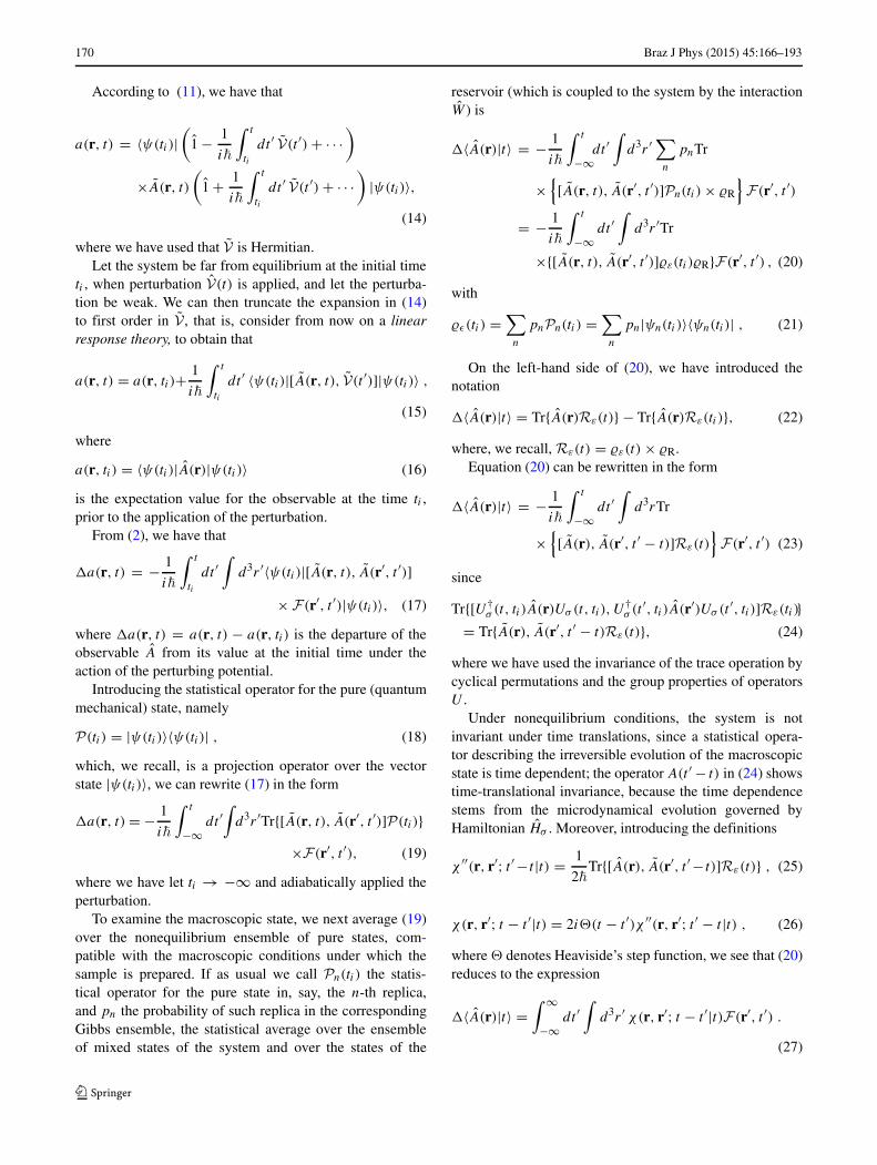
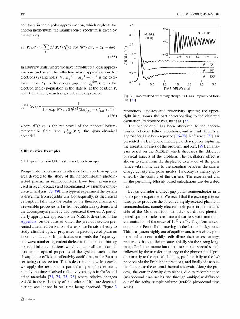
Pump-probe experiments in ultrafast laser spectroscopy, anarea devoted to the study of the nonequilibrium photoin-jected plasma in semiconductors, have been extensivelyused in recent decades and accompanied by a number of the-oretical analysis [73–89]. In a typical experiment the systemis driven far from equilibrium. Consequently, its theoreticaldescription falls into the realm of the thermodynamics ofirreversible processes in far-from-equilibrium systems, andthe accompanying kinetic and statistical theories. A partic-ularly appropriate approach is the NESEF, described in theAppendix, on the basis of which the previous section pre-sented a detailed derivation of a response function theory tostudy ultrafast optical properties in photoinjected plasmasin semiconductors. In particular, one needs the frequency-and wave number-dependent dielectric function in arbitrarynonequilibrium conditions, which contains all the informa-tion on the optical properties of the system, such as theabsorption coefficient, reflectivity coefficient, or the Ramanscattering cross section. This is described below. Moreover,we apply the results to a particular type of experiment,namely the time-resolved reflectivity changes in GaAs andother materials [74, 75, 75, 76] where relative changesR/R in the reflectivity of the order of 10−7 are detected,distinct oscillations in real time being observed. Figure 3
0.0
0.6
1.2
1.8
2.4
3.0
3.6
(10−
4 )
TIME DELAY (ps)
i-GaAs(100)
= 45
= 90
= 135
8.8 THz
-0.05
0.00
0.05
0 0.4 0.8 1.2 1.6 2.0
0 0.5 1.0 1.5 2.0 2.5 3.0
Fig. 3 Time-resolved reflectivity changes in GaAs. Reproduced fromRef. [73]
reproduces time-resolved reflectivity spectra; the upper-right inset shows the part corresponding to the observedoscillation, as reported by Cho et al. [73].
The phenomenon has been attributed to the genera-tion of coherent lattice vibrations, and several theoreticalapproaches have been reported [76–78]. Reference [77] haspresented a clear phenomenological description capturingthe essential physics of the problem, and Ref. [79], an anal-ysis based on the NESEF, which discusses the differentphysical aspects of the problem. The oscillatory effect isshown to stem from the displacive excitation of the polarlattice vibrations, due to the coupling between the carriercharge density and polar modes. Its decay is mainly gov-erned by the cooling of the carriers. The experiment andall the pertaining NESEF-based calculations are describednext.
Let us consider a direct-gap polar semiconductor in apump-probe experiment. We recall that the exciting intenselaser pulse produces the so-called highly excited plasma insemiconductors, namely electron-hole pairs in the metallicside of the Mott transition. In other words, the photoin-jected quasi-particles are itinerant carriers with minimumconcentration of the order of 1016 cm−3. They form a two-component Fermi fluid, moving in the lattice background.This is a system highly out of equilibrium, in which the pho-toexcited carriers rapidly redistribute their excess energy,relative to the equilibrium state, chiefly via the strong long-range Coulomb interaction (pico- to subpico-second scale),followed by the transfer of energy to the phonon field (pre-dominantly to the optical phonons, preferentially to the LOphonons via the Frohlich interaction), and finally via acous-tic phonons to the external thermal reservoir. Along the pro-cess, the carrier density diminishes, due to recombination(nanosecond time scale) and through ambipolar diffusionout of the active sample volume (tenfold picosecond timescale).
Braz J Phys (2015) 45:166–193 183
A probe interacting weakly with the HEPS generates anoptical response, namely the reflectivity of the incominglaser photons with frequency ω and wave vector Q. Fromthe theoretical point of view, as already noticed, the mea-surement is described by correlation functions in responsefunction theory. The usual application in normal probeexperiments on a system initially in equilibrium had a longhistory of success. A practical, elegant treatment employedthe double-time (equilibrium) thermodynamic Green func-tions method [67, 68]. To describe a pump-probe experi-ment, we have to apply an analogous theory to a systemwhose macroscopic state is out of equilibrium and evolvesin time as a result of dissipative processes that develop whilethe sample is probed. More specifically, we apply the theorydiscussed in the previous section and recall that the responsefunction theory for nonequilibrium systems needs be cou-pled to the kinetic theory that describes the evolution of thenonequilibrium state of the system. Here, we follow thisapproach to study the reflectivity experiments of Ref. [73].
The reflectivity R(ω, Q|t), which is time-dependentbecause it changes as the macrostate of the out-of-equilibrium system evolves, is related to the index ofrefraction η(ω, Q|t) + iκ(ω, Q|t) through the well-knownexpression
R(ω, Q|t) = [η(ω, Q|t) − 1]2 + [κ(ω, Q|t)]2
[η(ω, Q|t) + 1]2 + [κ(ω, Q|t)]2 , (157)
and the refraction index is related to the time-dependentfrequency- and wave vector-dependent dielectric functionby the equation
ε(ω, Q|t) = ε′(ω, Q|t) + iε′′(ω, Q|t)= [η(ω, Q|t) + iκ(ω, Q|t)]2 , (158)
where t denotes the measurement time; and η and ε′, andκ and ε′′ are the real and imaginary parts of the refractionindex and of the dielectric function, respectively.
The dielectric function depends on the frequency andthe wave vector of the radiation, and its time dependencereflects the evolution of the nonequilibrium plasma dur-ing the experiment. It is our task, therefore to calculatethis dielectric function in the nonequilibrium state of thesystem. From Maxwell’s equations in material media, thatis, Maxwell’s equations averaged over the nonequilibriumstatistical ensemble, we have that
ε−1(ω, Q|t) − 1 = n(ω, Q|t)r(ω, Q)
, (159)
where r(ω, Q) is the amplitude of a probe charge den-sity with frequency ω and wave vector Q, and n(ω, Q|t) isthe induced polarization-charge density of the carriers andlattice in the media. As we have shown the latter can be
calculated by response function theory for systems that arefar from equilibrium, a problem quite similar to the calcu-lation of the time-resolved Raman scattering cross section[70], and related to the nonequilibrium-thermodynamicGreen functions, as we now proceed to describe.
The formalism in Section 4, 98a and 98b, yields thefollowing expression for ε(ω, Q|t):
ε−1(ω, Q) − 1 = V (Q) [Gcc(ω, Q) + Gci(ω, Q)
+Gic(ω, Q) + Gii(ω, Q)] , (160)
where the Green functions are given by the equations
Gcc(ω, Q) = 〈〈nc(Q) ; n†c(Q)| ω; t〉〉 , (161)
Gci(ω, Q) = 〈〈nc(Q) ; n†i (Q)| ω; t〉〉 , (162)
Gic(ω, Q) = 〈〈ni(Q) ; n†c(Q)| ω; t〉〉 , (163)
Gii(ω, Q) = 〈〈ni(Q) ; n†i (Q)| ω; t〉〉 , (164)
where V (Q) = 4πne2/V ε0Q2 is the matrix element of
the Coulomb potential in plane-wave states and nc(Q),and ni (Q), refer to the Q-wavevector Fourier transformof the operators for the carrier charge densities and thepolarization charge of longitudinal optical phonons, respec-tively. The time-dependent distribution functions for thecarrier and phonon states make the results dependent onthe evolving nonequilibrium macroscopic state. They haveto be derived, therefore, within the kinetic theory in theNESEF. The first fundamental step is to choose the setof variables deemed appropriate for the description of themacroscopic state of the system. A first set of variableshas to comprise the carrier densities and energies and thephonon population functions, along with the set of associ-ated nonequilibrium-thermodynamics variables that, as wehave seen, can be interpreted as a reciprocal carrier quasi-temperatures and quasi-chemical potentials, and reciprocalphonon quasi-temperatures, one for each mode [64, 80–83].In the case under study, we need to add, on the basis ofthe information provided by the experiment, the amplitudesof the LO-lattice vibrations and the carrier charge density:the former because it is clearly present in the experimentaldata (the reflectivity oscillations) and the latter because ofthe LO-phonon-plasma coupling, clearly present in Ramanscattering experiments [84, 85]). Consequently, the chosenbasic set of dynamical quantities is
{Hc, Ne, Nh, nekp, nh
kp, νq, aq, a†q, HB} , (165)

184 Braz J Phys (2015) 45:166–193
where
Hc =∑
k
[εe
k c†k ck + εh
k h†−k h−k
], (166)
νq = a†q aq , (167)
Ne =∑
k
c†kck , Nh =
∑k
h†−k h−k , (168)
nekp = c
†k+pck , nh
kp = h−k−ph†−k , (169)
where c (c†), h (h†), and a (a†) annihilate (create) electron,hole, and LO-phonon states, respectively, and k, p, q runover the Brillouin zone. We use the effective mass approxi-mation and deal with the Coulomb interaction in the randomphase approximation, so that εe
k = EG + �2|k|2/2m∗
e andεh
k = �2|k|2/2m∗
h. Finally, HB is the Hamiltonian of thelattice vibrations other than the LO mode.
For the NESEF-nonequilibrium-thermodynamic vari-ables associated with the quantities in (165), we have that
{β∗c (t), −β∗
c (t)μ∗e (t), −β∗
c (t)μ∗h(t), F e
kp(t), F hkp(t),
�ωqβ∗q(t), ϕq(t), ϕ∗
q(t), β0}, (170)
respectively, where μ∗e and μ∗
h are the quasi-chemicalpotentials for electrons and for holes; we write β∗
c (t) =1/kBT ∗
c (t), which defines the carrier quasi-temperature T ∗c ;
β∗q(t) = 1/kBT ∗
q (t), which defines the LO-phonon quasi-temperature for each mode (ωq is the dispersion relation);and β0 = 1 / kB T0 where T0 is the thermal reservoir temper-ature. We indicate the corresponding macrovariables, thatis, those defining the nonequilibrium-thermodynamic Gibbsspace as
{Ec(t), n(t), n(t), nekp(t), nh
kp(t), νq(t), 〈aq |t〉,〈a†
q|t〉 = 〈aq|t〉∗, EB}, (171)
which are the statistical average of the quantities of (165),that is
Ec(t) = Tr{Hc �ε(t) × �R
}, (172)
n(t) = Tr{Ne(h) �ε(t) × �R
}, (173)
and so on, where �R is the stationary statistical distributionof the reservoir and n(t) is the carrier density, which is equalfor electrons and for holes since they are produced in pairs,in the intrinsic semiconductor. The volume of the activeregion of the sample (where the laser beam is focused) istaken equal to be unitary, for simplicity.
Next, we have to derive the equation of evolution for thebasic variables characterizing the nonequilibrium macro-scopic state of the system and, from them, the evolution of
the nonequilibrium-thermodynamic variables. This is doneaccording to the generalized NESEF-based nonlinear quan-tum transport theory [12, 16], in the second-order approx-imation in relaxation theory. The second-order approxima-tion retains only two-body collisions. Since memory andvertex corrections are neglected, this is the Markovian limitof the theory. It is sometimes referred to as the quasi-linearapproximation in relaxation theory [65, 66], a name weavoid because the word “linear”, which refers to the lowestorder in dissipation, is misleading, given that the equationsare highly nonlinear.
The NESEF-auxiliary (“instantaneously frozen”) statis-tical operator is in the present case given, in terms of thevariables of (165), and the nonequilibrium-thermodynamicvariables in (170), by the expression
�(t, 0) = exp{
− φ(t)−β∗c (t)[Hc−μ∗
e(t) Ne−μ∗h(t) Nh]
−∑kp
[F ekp(t) ne
kp(t) + F hkp(t) nh
kp(t)]
−∑
q
[β∗q(t) �ωq νq+ϕq(t) aq+ϕ∗
q(t) a†q]
−β0 HB
}, (174)
where φ(t) ensures the normalization of �(t, 0).Using this statistical operator, the Green functions that
define the dielectric function [cf. (160)] can be calculated.This is an arduous task, which calls for the evaluation of theoccupation functions
fk(t) = Tr{c†kck�ε(t)}, (175)
which depend on the variables of (170).The time evolution of the resulting (nonequilibrium)
carrier quasi-temperature T ∗c is shown in Fig. 4.
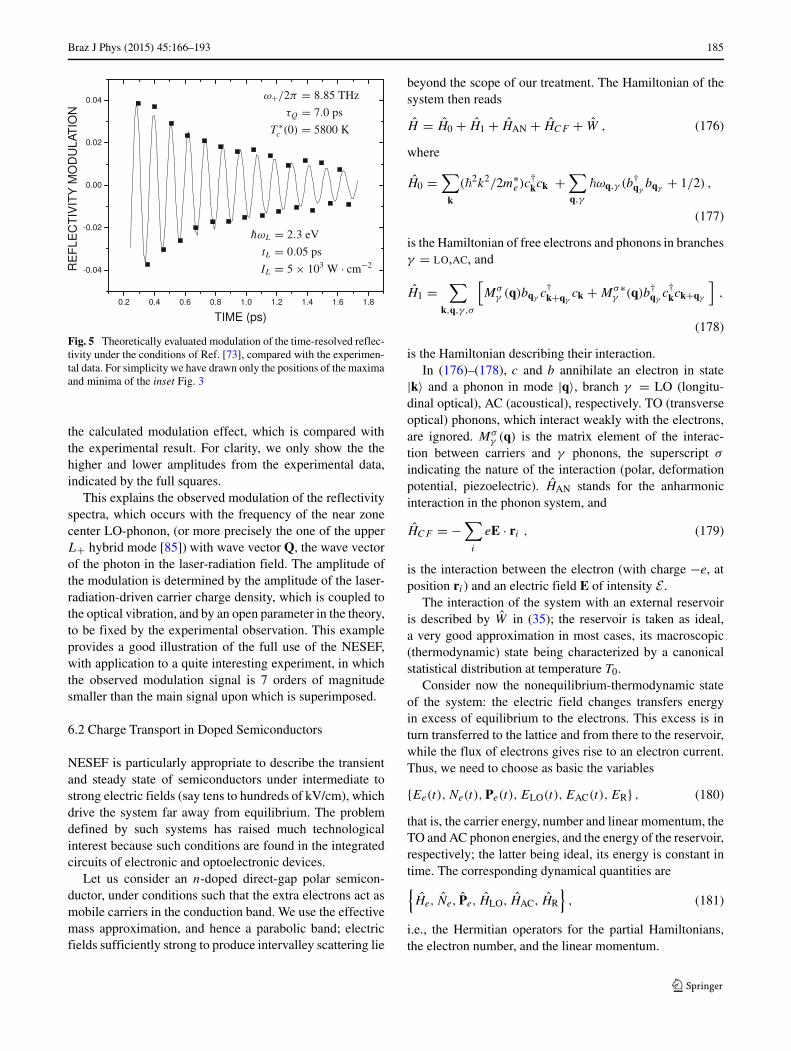
Figure 5, in which the only adjustable parameter is theamplitude—to fix which we fit the first maximum—shows
Fig. 4 Evolution of the carrier quasi-temperature, calculated under theconditions of the experiment in Fig. 3
Braz J Phys (2015) 45:166–193 185
Fig. 5 Theoretically evaluated modulation of the time-resolved reflec-tivity under the conditions of Ref. [73], compared with the experimen-tal data. For simplicity we have drawn only the positions of the maximaand minima of the inset Fig. 3
the calculated modulation effect, which is compared withthe experimental result. For clarity, we only show the thehigher and lower amplitudes from the experimental data,indicated by the full squares.
This explains the observed modulation of the reflectivityspectra, which occurs with the frequency of the near zonecenter LO-phonon, (or more precisely the one of the upperL+ hybrid mode [85]) with wave vector Q, the wave vectorof the photon in the laser-radiation field. The amplitude ofthe modulation is determined by the amplitude of the laser-radiation-driven carrier charge density, which is coupled tothe optical vibration, and by an open parameter in the theory,to be fixed by the experimental observation. This exampleprovides a good illustration of the full use of the NESEF,with application to a quite interesting experiment, in whichthe observed modulation signal is 7 orders of magnitudesmaller than the main signal upon which is superimposed.
6.2 Charge Transport in Doped Semiconductors
NESEF is particularly appropriate to describe the transientand steady state of semiconductors under intermediate tostrong electric fields (say tens to hundreds of kV/cm), whichdrive the system far away from equilibrium. The problemdefined by such systems has raised much technologicalinterest because such conditions are found in the integratedcircuits of electronic and optoelectronic devices.
Let us consider an n-doped direct-gap polar semicon-ductor, under conditions such that the extra electrons act asmobile carriers in the conduction band. We use the effectivemass approximation, and hence a parabolic band; electricfields sufficiently strong to produce intervalley scattering lie
beyond the scope of our treatment. The Hamiltonian of thesystem then reads
H = H0 + H1 + HAN + HCF + W , (176)
where
H0 =∑
k
(�2k2/2m∗e)c
†kck +
∑q,γ
�ωq,γ (b†qγ
bqγ + 1/2) ,
(177)
is the Hamiltonian of free electrons and phonons in branchesγ = LO,AC, and
H1 =∑
k,q,γ ,σ
[Mσ
γ (q)bqγ c†k+qγ
ck + Mσ∗γ (q)b†
qγc
†kck+qγ
],
(178)
is the Hamiltonian describing their interaction.In (176)–(178), c and b annihilate an electron in state
|k〉 and a phonon in mode |q〉, branch γ = LO (longitu-dinal optical), AC (acoustical), respectively. TO (transverseoptical) phonons, which interact weakly with the electrons,are ignored. Mσ
γ (q) is the matrix element of the interac-tion between carriers and γ phonons, the superscript σ
indicating the nature of the interaction (polar, deformationpotential, piezoelectric). HAN stands for the anharmonicinteraction in the phonon system, and
HCF = −∑
i
eE · ri , (179)
is the interaction between the electron (with charge −e, atposition ri) and an electric field E of intensity E .
The interaction of the system with an external reservoiris described by W in (35); the reservoir is taken as ideal,a very good approximation in most cases, its macroscopic(thermodynamic) state being characterized by a canonicalstatistical distribution at temperature T0.
Consider now the nonequilibrium-thermodynamic stateof the system: the electric field changes transfers energyin excess of equilibrium to the electrons. This excess is inturn transferred to the lattice and from there to the reservoir,while the flux of electrons gives rise to an electron current.Thus, we need to choose as basic the variables
{Ee(t), Ne(t), Pe(t), ELO(t), EAC(t), ER} , (180)
that is, the carrier energy, number and linear momentum, theTO and AC phonon energies, and the energy of the reservoir,respectively; the latter being ideal, its energy is constant intime. The corresponding dynamical quantities are{He, Ne, Pe, HLO, HAC, HR
}, (181)
i.e., the Hermitian operators for the partial Hamiltonians,the electron number, and the linear momentum.
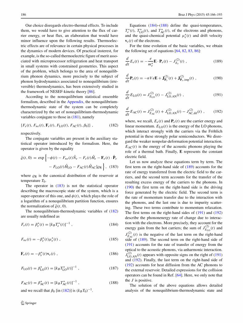
186 Braz J Phys (2015) 45:166–193
Our choice disregards electro-thermal effects. To includethem, we would have to give attention to the flux of car-rier energy, or heat flux, an elaboration that would haveminor influence upon the following results. Thermoelec-tric effects are of relevance in certain physical processes inthe dynamics of modern devices. Of practical insterest, forexample, is the so-called thermoelectric figure of merit asso-ciated with microprocessor refrigeration and heat transportin small systems with constrained geometries. This aspectof the problem, which belongs to the area of nonequilib-rium phonon dynamics, more precisely to the subject ofphonon hydrodynamics associated to nonequilibrium (irre-versible) thermodynamics, has been extensively studied inthe framework of NESEF-kinetic theory [86].
According to the nonequilibrium statistical ensembleformalism, described in the Appendix, the nonequilibrium-thermodynamic state of the system can be completelycharacterized by the set of nonequilibrium-thermodynamicvariables conjugate to those in (181), namely
{Fe(t), Fne(t), Fe(t), FLO(t), FAC(t), β0}} , (182)
respectively.The conjugate variables are present in the auxiliary sta-
tistical operator introduced by the formalism. Here, theoperator is given by the equality
�(t, 0) = exp{−φ(t) − Fne(t)Ne − Fe(t)He − Fe(t) · Pe
− FLO(t)HLO − FAC(t)HAC]�R
}, (183)
where �R is the canonical distribution of the reservoir attemperature T0.
The operator in (183) is not the statistical operatordescribing the macroscopic state of the system, which is asuper-operator of this one, and φ(t), which plays the role ofa logarithm of a nonequilibrium partition function, ensuresthe normalization of �(t, 0).
The nonequilibrium-thermodynamic variables of (182)are usually redefined as
Fe(t) = β∗e (t) = [kBT ∗
e (t)]−1 , (184)
Fne(t) = −β∗e (t)μ∗
e (t) , (185)
Fe(t) = −β∗e (t)ve(t) , (186)
FLO(t) = β∗LO(t) = [kBT ∗
LO(t)]−1 , (187)
FAC(t) = β∗AC(t) = [kBT ∗
AC(t)]−1 , (188)
and we recall that β0 [in (182)] is (kBT0)−1.
Equations (184)–(188) define the quasi-temperatures,T ∗
e (t), T ∗LO(t), and T ∗
AC(t), of the electrons and phonons,and the quasi-chemical potential μ∗
e(t) and drift velocityve(t) of the electrons.
For the time evolution of the basic variables, we obtainthe following set of equations [64, 82, 83, 86]:
d
dtEe(t) = − e
m∗e
E · Pe(t) − J(2)Ee
(t) , (189)
d
dtPe(t) = −nV eE + J(2)
Pe(t) + J(2)
Pe,imp(t) , (190)
d
dtELO(t) = J
(2)ELO
(t) − J(2)LO,AN(t) , (191)
d
dtEAC(t) = J
(2)EAC
(t) + J(2)LO,AN(t) − J
(2)AC,dif(t) , (192)
where, we recall, Ee(t) and Pe(t) are the carrier energy andlinear momentum. ELO(t) is the energy of the LO phonons,which interact strongly with the carriers via the Frohlichpotential in these strongly polar semiconductors. We disre-gard the weaker nonpolar-deformation potential interaction.EAC(t) is the energy of the acoustic phonons playing therole of a thermal bath. Finally, E represents the constantelectric field.
Let us now analyze these equations term by term. Thefirst term on the right-hand side of (189) accounts for therate of energy transferred from the electric field to the car-riers, and the second term accounts for the transfer of theresulting excess energy of the carriers to the phonons. In(190) the first term on the right-hand side is the drivingforce generated by the electric field. The second term isthe rate of momentum transfer due to the interaction withthe phonons, and the last one is due to impurity scatter-ing. These two terms contribute to momentum relaxation.The first terms on the right-hand sides of (191) and (192)describe the phononenergy rate of change due to interac-tion with the electrons. More precisely, they account for theenergy gain from the hot carriers; the sum of J
(2)ELO
(t) and
J(2)EAC
(t) is the negative of the last term on the right-handside of (189). The second term on the right-hand side of(191) accounts for the rate of transfer of energy from theoptical to the acoustic phonons, via anharmonic interaction.J
(2)LO,AN(t) appears with opposite signs on the right of (191)
and (192). Finally, the last term on the right-hand side of(192) accounts for heat diffusion from the AC phonons tothe external reservoir. Detailed expressions for the collisionoperators can be found in Ref. [64]. Here, we only note thatthe J is positive.
The solution of the above equations allows detailedanalysis of the nonequilibrium-thermodynamic state and

Braz J Phys (2015) 45:166–193 187
transport properties of these materials. Let us consider firstthe III-nitride compounds, which nowadays are raising par-ticular interest because they have potential application inlasers and diodes emitting in the blue and ultraviolet region(see, for example, Refs. [87, 88]).
Let us consider the steady state, which is very rapidlyestablished, in the time scale of 100 fs, because the strongFrohlich interaction raises the rate of energy transfer fromcarriers to LO phonons so that it quickly becomes equalto the rate of energy pumped into the system by theexternal field, of intensity E , even at high fields. Thedynamics is then characterized by the time-independentquasi-temperature, T ∗
e , drift velocity, ve, and quasi-chemicalpotential, μ∗
e , all pertaining to the electron system, andthe LO-phonon quasi-temperature T ∗
LO and the AC phononquasi-temperature T ∗
AC. Figure 6 shows the electric-fielddependence of T ∗
e ; Fig. 7 displays the electric-field depen-dence for the drift velocity for n-doped GaN, with n =1017 cm−3. The quasi-chemical potential is determined bythe concentration and electron quasi-temperature. The devi-ations of T ∗
LO and T ∗AC from the equilibrium value are small
and can be neglected.We can now proceed to calculate the light scattering cross
section by electrons under the electric field E . Taking intoaccount that the interaction of electrons and radiation isgiven by
VERQ = G(Q)nQ + H.c. , (193)
where �Q is the momentum of the photon, G(Q) is thematrix element of the interaction, and
nQ =∑
k
nkQ =∑
k
c†k+Qck , (194)
0 10 20 30 40 50 60 70 80 90 100
300
400
500
600
700
800
900
n-GaN
CA
RR
IER
QU
AS
ITE
MP
ER
AT
UR
E (
K)
ELECTRIC FIELD (kV/cm)
Fig. 6 Electric-field dependence of the quasi-temperature T ∗e in the
steady state for n-doped GaN. We have chosen m∗ = 0.19m0,ε0 = 9.5, carrier concentration n = 1017 cm−3, and the thermal bathtemperature T0 = 300 K. After Ref. [89]
0 10 20 30 40 50 60 70 80 90 1000.0
0.4
0.8
1.2
1.6
2.0
2.4 n-GaN
CA
RR
IER
DR
IFT
VE
LOC
ITY
(10
7 cm/s
)
ELECTRIC FIELD (kV/cm)
Fig. 7 Electric-field dependence of the electron drift velocity in thesteady state for n-doped GaN. The experimental conditions are thosein the caption of Fig. 6. After Ref. [89]
to first order in the scattering operator the cross section in(143) is given by the expression
d2σ(Q, ω)
dωd�= V 2
(2π�)3
�ω2
c4|G(Q)|2
∞∫
−∞dτe−iωτ
×Tr{n†QnQRε}. (195)
We recall that the system is in steady state, and that thetwo integrals in (143) can be combined as above. We haveused that g(ω) = �
3ω2/c3 and v0 = c.We can now use the generalized fluctuation-dissipation
theorem of Section 3. We keep only the relevant part definedin that section, i.e., substitute R for Rε in (183). In thesteady state, we then find that
d2σ(Q, ω)
dωd�∼ [1 − e−β∗(�ω−Q·ve)]−1Im{ε−1(Q, ω|E)} ,
(196)
In (196), ε(Q, ω|E) is the dielectric function at the wavevector Q and frequency ω (i.e., the momentum and energytransfer in the scattering event, as we have seen), since weuse that
ε(Q, ω|E) = 1−V(Q)∑
k
f (k + Q|E) − f (k|E)
E(k + Q) − E(k) − �(ω + is),
(197)
where E(k) = �2k2/2m∗
e , in the effective mass approxima-tion, and s is a positive infinitesimal; we let s → +0 toobtain the real and imaginary parts of ε(Q, ω) = ε1(Q, ω)+iε2(Q, ω).
Equation (197) has the form of the Lindhardt (RPA)dielectric function, here written in terms of the nonequilib-rium distribution functions f (k|E). The latter have the form
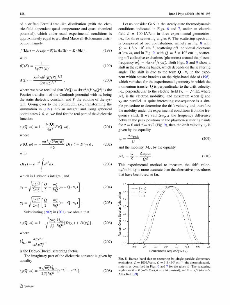
188 Braz J Phys (2015) 45:166–193
of a drifted Fermi-Dirac-like distribution (with the elec-tric field-dependent quasi-temperature and quasi-chemicalpotential), which under usual experimental conditions isapproximately equal to a drifted Maxwell-Boltzmann distri-bution, namely
f (k|E) = A exp{−β∗e (E)[E(k) − E · �k]} , (198)
with
β∗e (E) = 1
kBT ∗(E), (199)
A(E) = 8π3n�3[β∗e (E)]3/2
(2πm∗e)
3/2, (200)
where we have recalled that V(Q) = 4πe2/(V ε0Q2) is the
Fourier transform of the Coulomb potential with ε0 beingthe static dielectric constant, and V the volume of the sys-tem. Going over to the continuum, i.e., transforming thesummation in (197) into an integral and using sphericalcoordinates k, θ , ϕ, we find for the real part of the dielectricfunction
ε1(Q, ω) = 1 − V(Q)
4π3F(Q, ω) , (201)
where
F(Q, ω) = −nπ3√
25m∗eβ
∗e
�Q[D(y1) + D(y2)] , (202)
with
D(y) = e−y2
y∫
0
ex2dx , (203)
which is Dawson’s integral, and
y1 =√
β∗e �
2
2m∗e
[Q
2+ m∗
e
�Q(ω − Q · ve)
], (204)
y2 =√
β∗e �
2
2m∗e
[Q
2− m∗
e
�Q(ω − Q · ve)
], (205)
Substituting (202) in (201), we obtain that
ε1(Q, ω) = 1 +√
2m∗e
β∗e
k2DH
�Q3 [D(y1) + D(y2)] , (206)
where
k2DH = 4πe2n
ε0kBT ∗e
, (207)
is the Debye-Huckel screening factor.The imaginary part of the dielectric constant is given by
equality
ε2(Q, ω) = π√
m∗ek
2DH
2β∗e �Q
3 [e−y22 − e−y2
1 ]. (208)
Let us consider GaN in the steady-state thermodynamicconditions indicated in Figs. 6 and 7, under an electricfield E = 100 kV/cm, in three experimental geometries,i.e., for three scattering angles θ . The scattering spectrumis composed of two contributions, namely in Fig. 8 withQ = 1.8 × 105 cm−1, scattering off individual electronsat low ω, and in Fig. 9, with Q = 5 × 104 cm−1, scatter-ing off collective excitations (plasmons) around the plasmafrequency ω2
p = 4πne2/ε0m∗e . Both Figs. 8 and 9 show a
shift in the scattering bands, which depends on the scatteringangle. The shift is due to the term Q · ve in the expo-nent within square brackets on the right-hand side of (196),which vanishes for the experimental geometry in which themomentum transfer Q is perpendicular to the drift velocity,i.e., perpendicular to the electric field (ve = MeE, whereMe is the electron mobility), and maximum when Q andve are parallel. A quite interesting consequence is a sim-ple procedure to determine the drift velocity and thereforethe mobility under the experimental conditions from the fre-quency shift. If we call ωpeak the frequency differencebetween the peak positions in the plasmon-scattering bandsfor θ = 0 and θ = π/2 (Fig. 9), then the drift velocity ve isgiven by the equality
ve = ωpeak
Q, (209)
and the mobility Me, by the equality
Me = ve
E = ωpeak
QE . (210)
This experimental method to measure the drift veloc-ity/mobility is more accurate than the alternative proceduresthat have been used so far.
Fig. 8 Raman band due to scattering by single-particle elementaryexcitations. E = 100 kV/cm, Q = 1.8×105 cm−1, the thermodynamicstate is as described in Figs. 6 and 7 for the given E . The scatteringangles are θ = 0 (solid line), θ = π/4 (dashed), and θ = π/2 (dotted).After Ref. [89]

Braz J Phys (2015) 45:166–193 189
Fig. 9 Raman band due to scattering by plasma excitations. The spec-ifications are as in the caption of Fig. 8, except that Q = 5×104 cm−1.After Ref. [89]
7 Final Remarks
We have presented a response function theory, accompaniedby a fluctuation dissipation theorem, and a theory of scat-tering adapted to deal with systems arbitrarily far removedfrom equilibrium, including time- and space-resolvedexperiments.
The theory was built within the framework of a Gibbs-style nonequilibrium statistical ensemble formalism. Thegeneral form of the generalized (space- and time-dependent)susceptibility is obtained in the form of space- and time-dependent correlation functions defined over the nonequi-librum ensemble. It is also dependent on the variablesthat characterized the nonequilibrium-thermodynamic stateof the system. The generalized susceptibility for the cor-responding experimental situation is therefore coupledto the equations of evolution of the nonequilibrium-thermodynamic variables. We have also presented a methodto calculate nonequilibrium-thermodynamic Green func-tions, that is, the extension to arbitrary nonequilibrium con-ditions of the Bogoliubov-Tyblikov thermodynamic Greenfunctions.
A fluctuation-dissipation theorem in the context ofthe nonequilibrium ensemble formalism was presented inSection 3, which is an extension to arbitrary nonequilibriumconditions of Kubo’s theorem.
In Section 5, we have presented a theory of scatteringfor scattering experiments on systems that are arbitrarily farremoved from equilibrium. A space- and time-dependentscattering cross section was obtained, which like the gener-alized susceptibility of response function theory, depends onthe nonequilibrium-thermodynamic state of the system. The
scattering cross section is therefore coupled to the equationsof evolution for the nonequilibrium variables.
Finally, Section 6 presented a few illustrative exam-ples. We applied the theory to the analysis of experimentalresults, namely, in ultrafast laser spectroscopy and chargetransport in doped polar semiconductors.
Acknowledgments The authors would like to acknowledge partialfinancial support received from the Sao Paulo State Research Agency(FAPESP), Goias State Research Agency (FAPEG), and the BrazilianNational Research Council (CNPq). The authors are CNPq ResearchFellows.
In Memoriam: With very sad feelings, we regret to report the pass-ing away of our dear colleague Prof. Dr. Aurea Rosas Vasconcellos,a genuine, devoted, and extremely competent teacher and researcherwith fervent dedication to Theoretical Physics in the Condensed Matterarea.
Appendix: The Nonequilibrium Statistical Operator
The construction of nonequilibrium statistical ensembles,that is, a nonequilibrium statistical ensemble formalism,NESEF for short [8–13], basically consisting of deriving anonequilibrium statistical operator (probability distributionin the classical case) has been attempted along several lines.In a brief summarized way, we describe the constructionof NESEF within a heuristic approach. In this context, sev-eral important points must be carefully taken into account ineach case under consideration:
1. Choice of the basic variables. The choices for equilib-rium and for nonequilibrium are different; for systemsin equilibrium, it suffices to consider the constants ofmotion. To choose the variables for systems out ofequilibrium, we must identify macroscopic processesand measurements and focus attention not only on theobservables, but also on the character and expectationsconcerning the evolution equations for these variables[12, 13, 90]. Although all observables—along with theircorrelations, in certain cases—must be dealt with at theinitial stage, as time elapses more and more contracteddescriptions become possible as Bogoliubov’s princi-ple of correlation weakening and the accompanyinghierarchy of relaxation times comes into play [91].
2. Irreversibility (or Eddington’s arrow of time). Concern-ing this facet of the problem, Rudolf Peierls has statedthat “In any theoretical treatment of transport problems,it is important to realize at what point the irreversibilityhas been incorporated. If it has not been incorporated,the treatment is wrong. A description of the situationthat preserves the reversibility in time is bound to givethe answer zero or infinity for any conductivity. If wedo not see clearly where the irreversibility is introduced,we do not clearly understand what we are doing” [92].

190 Braz J Phys (2015) 45:166–193
3. Historicity. Proper treatment must incorporate the entirepast dynamics of the system, or historicity effects, froma starting description of the macrostate of the samplein the experiment under study, say at t0, up to the timet when a measurement is performed. This is a quiteimportant point in the case of dissipative systems, asemphasized among others by John Kirkwood, MelvinGreen, Robert Zwanzig, and Hazime More [36–40]. Itimplies that the history of the system is not merelythe series of events involving the system, but the seriesof transformations along time through which the sys-tem progressively comes into being at the measurementtime t , through the evolution governed by the laws ofmechanics [93]
Concerning the choice of the basic variables, in con-trast with the equilibrium case, immediately after the openN -particle system, in contact with external sources andreservoirs, has been driven out of equilibrium, it becomesnecessary to describe its state in terms of all its observ-ables and, in certain instances, to introduce direct andcross-correlations. As time elapses, however, Bogoliubov’sprinciple of correlation weakening allows us to introduceincreasing contractions of descriptions.
On the question of irreversibility, Nicolai S. Krylov[42] considered that there always exists a physical interac-tion between the measured system and the external worldthat is constantly “jolting” the system out of its exactmicrostate. Thus, the instability of trajectories and theunavoidable finite interaction with the outside would guar-antee the validity of a “crudely prepared” macroscopicdescription. In the absence of a proper way to introducethis effect, one needs to resort to the interventionist’sapproach, which is grounded on this ineluctable randomiza-tion process and leads to the asymmetric evolution of themacrostate.
The “intervention” consists of introducing in the Liou-ville equation for the statistical operator of the otherwiseisolated system, a special source accounting for Krylov’s“jolting” effect, in the following form (for the logarithm ofthe statistical operator):
∂
∂tlnRε(t)+ 1
i�[lnRε(t), H ] = −ε[lnRε(t)−ln R(t, 0)],
(211)
where ε (effectively the reciprocal of a relaxation time)is taken to go to +0 after the average values have beencomputed.
This mathematically inhomogeneous term, in the oth-erwise normal Liouville equation, implies a continuoustendency to relax the statistical operators toward a referen-tial distribution, R, which, as discussed below, representsan instantaneous quasi-equilibrium condition.
We can regard (211) as a regular Liouville equation withan infinitesimal source, which provides Bogoliubov’s sym-metry breaking of time reversal and justifies disregardingthe advanced solutions [8, 12, 13, 94, 95]. This is describedby a Poisson distribution and the result at time t is obtainedby averaging over all t ′ in the interval (t0, t), since thesolution of (211) is
Rε(t) = exp
⎧⎨⎩−S(t, 0) +
t∫
t0
dt ′eε(t ′−t ) d
dt ′S(t ′, t ′ − t)
⎫⎬⎭ ,
(212)
where
S(t, 0) = − ln R(t, 0), (213)
S(t ′, t ′ − t) = exp
{− 1
i�(t ′ − t)H
}S(t ′, 0)
× exp
{1
i�(t ′ − t)H
}, (214)
and the initial-time condition at time t0, when the formalismbegins to be applied, is
Rε(t0) = R(t0, 0). (215)
The first time variables in the arguments of both R and S
refer to the evolution of the nonequilibrium-thermodynamicvariables, and the second time variables, to the time evo-lution of the dynamical variables, both of which affect theoperator.
The time t0, which starts the statistical description, isusually taken in the remote past (t0 → −∞), which intro-duces an adiabatic switching-on of the relaxation process. In(212), the time integration in the interval (t0, t) is weightedby the kernel exp{ε(t ′ − t)}. The presence of this ker-nel introduces a kind of evanescent history as the systemmacrostate evolves toward the future from the boundarycondition of (215) at time (t0 → −∞), a fact evidencedin the resulting kinetic theory [8–13, 16, 38], which clearlyindicates that a fading memory of the dynamical process hasbeen introduced. The statistical operator can be written inthe form
Rε(t) = R(t, 0) + R′ε(t) . (216)
involving the auxiliary probability distribution R(t, 0), plusR′
ε(t), which contains the historicity and irreversibilityeffects.
In most cases, we can consider the system as composedof the system of interest, i.e., the system on which we areperforming an experiment, and ideal reservoirs in contactwith it. Therefore, we can write the expression
R(t, 0) = �(t, 0) × �R . (217)
Braz J Phys (2015) 45:166–193 191
and
Rε(t) = �ε(t) × �R , (218)
where �ε(t) is the statistical operator of the nonequilibriumsystem, � the auxiliary one, and �R the stationary operatorfor the ideal reservoirs, with �ε(t) then given by the equality
�ε(t) = exp
⎧⎨⎩−S(t, 0) +
t∫
−∞dt ′eε(t ′−t ) d
dt ′S(t ′, t ′ − t)
⎫⎬⎭ ,
(219)
with the initial value �(t0, 0) (t0 → −∞), and where
S(t, 0) = − ln �(t, 0) , (220)
Finally, we have to provide the auxiliary statistical oper-ator �(t, 0). This operator, sometimes dubbed the quasi-equilibrium statistical operator, expresses an instantaneousdistribution at time t describing a “frozen” equilibrium thatdefines the macroscopic state of the system at that moment.On the basis of this notion (or, alternatively, via the vari-ational procedure [12, 13, 96–104]) and considering thedescription of the system nonequilibrium state in terms ofthe basic set of dynamical variables Pj , the reference orinstantaneous quasi-equilibrium statistical operator is takenas a canonical-like one given by the equality
�(t, 0) = exp{−φ(t) −n∑j
Fj (t)Pj } , (221)
with φ(t) ensuring the normalization of � and playing therole of a logarithm of a partition function, say, φ(t) =ln Z(t).
Moreover, in (221), Fj is the nonequilibrium-thermodynamic variable associated with the basicdynamical variable Pj . The nonequilibrium-thermodynamicspace of states is composed by the basic variables{Qj(t)}, which comprise the averages of the {Pj } over thenonequilibrium ensemble, namely,
Qj(t) = Tr{Pj�ε(t)} , (222)
which are then functionals of the {Fj(t)} and there followthe equations of state
Qj(t) = − δφ(t)
δFj (t)= −δ ln Z(t)
δFj (t), (223)
where δ denotes functional derivative.Moreover,
S(t) = Tr{ ˆS(t, 0)�(t, 0)} = −Tr{�(t, 0) ln �(t, 0)} , (224)
is the so-called informational entropy characteristic ofthe distribution �, a functional of the basic variables{Qj(t)}, in terms of which the following alternative form ofthe equations of state can be written:
− δS(t)
δQj (t)= Fj (t) , (225)
References
1. R. Kubo, Oppening address at the Oji seminar. Prog. Theor. Phys.(Japan) 64 (1978)
2. S. Stix, Little big science: an overview, and articles thereafter. Sci.Am. 285(3), 26 (2001)
3. F. Family, T. Vicsek, Dynamics of Fractal Surfaces (World Scien-tific, Singapore, 1991)
4. R. Luzzi, A.R. Vasconcellos, J.G. Ramos, Riv. Nuovo Cimento30(3), 95 (2007)
5. A. Renyi, On measures of entropy and information, in Proc. 4thBerkeley Symposium Math. Stat. Prob., vol 1 (1961), p. 547
6. A. Renyi, Probability Theory (North Holland, Amsterdam, 1970)7. P. Jizba, T. Arimitzu, Ann. Phys. (NY) 312, 17 (2004)8. D.N. Zubarev, Non Equilibrium Statistical Thermodynamics
(Consultants Bureau, New York, 1974)9. D.N. Zubarev, V. Morozov, G. Ropke, Statistical Mechanics of
Non Equilibrium Processes I (Academie Verlag-Wiley VCH,Berlin, 1996)
10. D.N. Zubarev, V. Morozov, G. Ropke, Statistical Mechanics ofNon Equilibrium Processes II (Academie Verlag-Wiley VCH,Berlin, 1997)
11. A. Akhiezer, S. Peletminskii, Methods of Statistical Physics (Perg-amon, Oxford, 1981)
12. R. Luzzi, A.R. Vasconcellos, J.G. Ramos, Predictive Statisti-cal Mechanics: A Non-equilibrium Ensemble Formalism (KluwerAcademic, Dordrecht, 2002)
13. R. Luzzi, A.R. Vasconcellos, J.G. Ramos, Riv. Nuovo Cimento29(2), 1–82 (2006)
14. M.H. Kalos, P.A. Whitlock, Monte Carlo Methods (Wiley, NewYork, 2007)
15. B.J. Adler, D.J. Tildesley, Computer Simulation of Liquids(Oxford University Press, Oxford, 1987)
16. L. Lauck, A.R. Vasconcellos, R. Luzzi, Phys. A 168, 789 (1990)17. C.G. Rodrigues, V.N. Freire, J.A.P. Costa, A.R. Vasconcellos, R.
Luzzi, Phys. Stat. Sol. (b) 216, 35 (1999)18. C.G. Rodrigues, A.R. Vasconcellos, R. Luzzi, V. Lemos, V.N.
Freire, Mater. Sci. Forum 338–342, 1579 (2000)19. A.R. Vasconcellos, R. Luzzi, C.G. Rodrigues, V.N. Freire, Appl.
Phys. Lett. 82, 2455 (2003)20. C.G. Rodrigues, V.N. Freire, A.R. Vasconcellos, R. Luzzi, Appl.
Phys. Lett. 76, 1893 (2000)21. C.G. Rodrigues, A.R. Vasconcellos, V.N. Freire, R. Luzzi, J. Appl.
Phys. 90, 1879 (2001)22. C.G. Rodrigues, A.R. Vasconcellos, V.N. Freire, R. Luzzi, J. Appl.
Phys. 95, 4914 (2004)23. C.G. Rodrigues, A.R. Vasconcellos, V.N. Freire, R. Luzzi, J. Appl.
Phys. 99, 073701 (2006)24. C.G. Rodrigues, A.R. Vasconcellos, V.N. Freire, R. Luzzi, J. Appl.
Phys. 102, 073714 (2007)25. C.G. Rodrigues, V.N. Freire, A.R. Vasconcellos, R. Luzzi, Braz. J.
Phys. 32(2A), 439 (2002)

192 Braz J Phys (2015) 45:166–193
26. C.G. Rodrigues, V.N. Freire, A.R. Vasconcellos, R. Luzzi, Braz. J.Phys. 36(2A), 255 (2006)
27. A.R. Vasconcellos, M.J.S.P. Brasil, R. Luzzi, A.A.P. Silva, A.H.S.Leite, J. Appl. Phys. 106, 043503 (2009)
28. C.G. Rodrigues, A.R. Vasconcellos, R. Luzzi, V.N. Freire, J. Phys.Condens. Matter 19, 346214 (2007)
29. C.G. Rodrigues, A.R. Vasconcellos, R. Luzzi, Phys. Status Solidi(b) 246(2), 417 (2009)
30. A.R.B. Castro, A.R. Vasconcellos, R. Luzzi, Rev. Scient. Inst. 81,073102 (2010)
31. C.G. Rodrigues, A.R. Vasconcellos, R. Luzzi, J. Appl. Phys. 108,033716 (2010)
32. A.R. Vasconcellos, A.R.B. Castro, C.A.B. Silva, R. Luzzi, AIPAdv. 3, 072106 (2013)
33. C.G. Rodrigues, A.R. Vasconcellos, R. Luzzi, J. Appl. Phys. 113,113701 (2013)
34. C.G. Rodrigues, A.R. Vasconcellos, V.N. Freire, R. Luzzi, J. Appl.Phys. 98, 043702 (2005)
35. C.G. Rodrigues, A.R. Vasconcellos, V.N. Freire, R. Luzzi, J. Appl.Phys. 98, 043703 (2005)
36. J.G. Kirkwood, J. Chem. Phys. 14, 180 (1946)37. M.S. Green, J. Chem. Phys. 20, 1281 (1952)38. H. Mori, I. Oppenheim, J. Ross, Some topics in quantum statis-
tics, in Studies in Statistical Mechanics I, ed. by J. de Boer, G.E.Uhlenbeck (North Holland, Amsterdam, 1962)
39. H. Mori, Progr. Theor. Phys. (Japan) 33, 423 (1965)40. R. Zwanzig, Statistical mechanics of irreversibility, in Lectures in
Theoretical Physics, ed. by W.E. Brittin, B.W. Downs, J. Downs,Vol. 3 (Wiley-Interscience, New York, 1961)
41. A. Salam, V.S. Vladimorov, A.A. Logunov, Theor. Math. Phys.92, 817 (1993)
42. N.S. Krylov, Works on The Foundations of Statistical Mechanics(Princeton University Press, Princeton, 1979)
43. S.V. Peletminski, A.A. Yatsenko, JETP 26, 773 (1968)44. D.N. Zubarev, V.P. Kalashnikov, Theor. Math. Phys. 96, 108
(1970)45. E.T. Jaynes, in Papers on Probability, Statistics and Statistical
Physics, ed. by R.D. Rosenkrantz (Reidel, Dordrecht, 1983)46. E.T. Jaynes, Predictive statistical mechanics, in Frontiers of Non
Equilibrium Statistical Physics, ed. by G.T. Moore, M.O. Scully(Plenum, New York, 1986), pp. 33–55
47. C.E. Shannon, Bell Sys. Tech. J. 27, 379–423 (1948)48. C.E. Shannon, W. Weaver, The Mathematical Theory of Commu-
nication (University of Illinois Press, Urbana, 1949)49. P.C. Martin, Measurements and correlation functions, in Many-
Body Physics, ed. by C.D. Witt, R. Balian (Gordon and Breach,New York, 1968), pp. 37–136
50. L. Hove, Phys. Rev. 95, 249 and 1374 (1954)51. H.J. Kreuzer, Non Equilibrium Thermodynamics and Its Statisti-
cal Foundations (Claredon, Oxford, 1981)52. V.P. Kalashnikov, Theor. Math. Phys. 9, 1003 (1971)53. V.P. Kalashnikov, Theor. Math. Phys. 35, 362 (1978)54. R. Luzzi, A.R. Vasconcellos, J. Stat. Phys. 23, 539 (1980)55. H. Nyquist, Phys. Rev. 32, 110 (1928)56. H.B. Callen, T.A. Welton, Phys. Rev. 83, 34 (1951)57. R. Kubo, J. Phys. Soc. Jpn. 12, 570 (1957)58. R. Kubo, Rep. Prog. Phys. 29, 255 (1966)59. R. Zon, E.G.D. Cohen, Phys. Rev. Lett. 91, 110601 (2003)60. D.J. Evans, D.J. Searles, Adv. Phys. 51, 1529 (2002)61. R. Luzzi, A.R. Vasconcellos, J. Casas-Vazquez, D. Jou, J. Chem.
Phys. 107, 7383 (1997)62. R. Luzzi, A.R. Vasconcellos, J. Casas-Vazquez, D. Jou, Phys. A
234, 699 (1997)
63. R. Luzzi, A.R. Vasconcellos, J. Casas-Vazquez, D. Jou, Phys. A248, 111 (1998)
64. C.G. Rodrigues, A.R. Vasconcellos, R. Luzzi, Transp. Theor. Stat.Phys. 29, 733 (2000)
65. V.P. Kalashnikov, Theor. Math. Phys. 9, 1003 (1972)66. V.P. Kalashnikov, Theor. Math. Phys. 35, 362 (1978)67. D.N. Zubarev, Uspekhi 3, 320 (1960)68. V.L. Tyablikov, Methods in the Quantum Theory of Magnetism
(Plenum, New York, 1974)69. J.R. Madureira, A.R. Vasconcellos, R. Luzzi, L. Lauck, Phys. Rev.
E 57, 3637 (1998)70. R. Luzzi, A.R. Vasconcellos, J. Raman Spectrosc. 10, 28 (1981)71. A.R. Vasconcellos, R. Luzzi, J. Raman Spectrosc. 14, 39 (1983)72. L. Hove, in Quantum Theory of Many-Particle Systems, ed. by L.
van Hove, N.M. Hugenholtz, L.P. Howland (Benjamin, New York,p. 1961
73. G.L. Cho, W. Kutt, H. Kurz, Phys. Rev. Lett. 65, 764 (1990)74. W. Albrecht, T. Kruse, H. Kurz, Phys. Rev. Lett. 69, 1451–1454
(1992)75. T. Pfeifer, W. Kutt, R. Scholz, Phys. Rev. Lett. 69, 3248 (1992)76. R. Scholz, T. Pfeifer, H. Kurz, Phys. Rev. B 47, 16229 (1993)77. H.J. Zeiger, J. Vidal, T.K. Cheng, E.P. Ippen, G. Dresselhaus, M.S.
Dresselhaus, Phys. Rev. B 45, 768 (1992)78. A.V. Kutnevsov, C.J. Stanton, Phys. Rev. Lett. 73, 3243 (1994)79. A.R. Vasconcellos, R. Luzzi, A.J. Madureira, J. Phys.: Condens.
Matter 12, 5325 (2000)80. A.C. Algarte, A.R. Vasconcellos, R. Luzzi, Phys. Rev. B 54, 11311
(1996)81. A.C. Algarte, A.R. Vasconcellos, R. Luzzi, Braz. J. Phys. 26, 543
(1996)82. C.G. Rodrigues, A.R. Vasconcellos, R. Luzzi, J. Phys. D: Appl.
Phys. 38, 3584–3589 (2005)83. C.G. Rodrigues, A.R. Vasconcellos, R. Luzzi, Solid State Com-
mun. 140, 135–140 (2006)84. P. Wolff, in Light Scattering Spectra of Solids, ed. by G.B. Wright
(Springer, New York, 1969)85. A. Mooradian, in Light Scattering Spectra of Solids, ed. by G.B.
Wright (Springer, New York, 1969)86. A.A.P. Silva, A.C. Algarte, A.R. Vasconcellos, R. Luzzi, J. Appl.
Phys. 90, 3973 (2001)87. N.M. Johnson, A.V. Nurmikko, S.P. DenBoars, Blue Diode Lasers.
Phys. Today 53(10), 31 (2000)88. C.G. Rodrigues, A.A.P. Silva, C.A.B. Silva, A.R. Vaconcellos,
J.G. Ramos, R. Luzzi, Braz. J. Phys. 40, 63–91 (2010)89. C.G. Rodrigues, A.R. Vasconcellos, R. Luzzi, Eur. Phys. J. B
72(1), 67 (2009)90. R. Zwanzig, Where we go from here?, in Perspectives in Statisti-
cal Mechanics, ed. by H.J. Raveche (North Holland, Amsterdam,1981)
91. N.N. Bogoliubov, Problems of a dynamical theory in statisticalphysics, in Studies in Statistical Physics, ed. by J. de Boer, G.E.Uhlenbeck (North Holland, Amsterdam, 1962)
92. R. Peierls, Some simple remarks on the basis of transport the-ory, in Lecture Notes in Physics, ed. by J. Ehlers, K. Hepp, H.A.Weidenmuller, Vol. 31 (Springer, Berlin, 1974)
93. H. Mori, I. Oppenheim, J. Ross, Some topics in quantum statis-tics, in Studies in Statistical Mechanics I, ed. by J. de Boer, G.E.Uhlenbeck (Amsterdam, North Holland, 1962)
94. N.N. Bogoliubov, Vol. 1, Lectures in Quantum Mechanics (Gor-don and Breach, New York, 1967)
95. N.N. Bogoliubov, Vol. 2, Lectures in Quantum Mechanics (Gor-don and Breach, New York, 1970)
96. W.M. Elsasser, Phys. Rev. 52, 987 (1937)
Braz J Phys (2015) 45:166–193 193
97. E.T. Jaynes, in Physics and Probability, ed. by W.T. Grandy,P.W. Milonni (Cambridge University Press, Cambridge, 1993),pp. 261–275
98. E.T. Jaynes, in Maximum Entropy and Bayesian Methods, ed. byW.T. Grandy, L.H. Schick (Kluwer Academic, Dordrecht, 1991),pp. 1–13
99. B. Robertson, Phys. Rev. 144, 151–161 (1966)100. B. Robertson, Phys. Rev. 160, 175–183 (1967)
101. E.T. Jaynes, Probability Theory: The Logic of Science (Cam-bridge University Press, Cambridge, 2002)
102. J. Bricmont, in Chance in Physics, ed. by J. Bricmont, et al.(Springer, Heidelberg, 2001)
103. J. Bricmont, Phys. Mag. 17, 159–208 (1995)104. J. Bricmont, Vol. 775, The Flight from Science and Reason,
Annals New York Academy of Sciences (NYAS, New York, 1996),pp. 131–175


![[R. Kubo,] Statistical Mechanics - An Adv. Course (BookZZ.org)](https://img.pdfslide.us/doc/110x75/5695d4741a28ab9b02a181a6/r-kubo-statistical-mechanics-an-adv-course-bookzzorg.jpg)