Embed Size (px)
Citation preview
Fully integrated modelling of surface-subsurface flow processes: quantifying in-stream and overland flow
generation mechanisms.
by Daniel Joseph Partington
BEng (Civil & Environmental) Hons, BSc (Maths and Computer Science)
Thesis submitted to The University of Adelaide School of Civil, Environmental & Mining Engineering in
fulfilment of the requirements for the degree of Doctor of Philosophy
Submitted December 2012
Copyright© December, 2012.


Contents
iii
Contents
Contents ............................................................................................................ iii
Abstract ............................................................................................................ vii
Statement of Originality .................................................................................. ix
Acknowledgements ........................................................................................... xi
List of Figures ................................................................................................. xiii
List of Tables ................................................................................................. xvii
1 Introduction ....................................................................................................... 1
1.1. Research Objectives ..................................................................................... 4
1.2. Thesis Overview .......................................................................................... 6
2 A hydraulic mixing-cell method to quantify the groundwater component
of streamflow within spatially distributed fully integrated surface water -
groundwater flow models (Paper 1) ................................................................ 9
2.1. Introduction ................................................................................................ 13
2.2. Existing methods for extracting streamflow generation components ........ 16
2.2.1. Summed exfiltration along the length of the stream ...................... 16
2.2.2. Tracer based hydrograph separation .............................................. 17
2.3. A hydraulic balance using a hydraulic mixing-cell method ...................... 19
2.3.1. Theory ............................................................................................ 19
2.3.2. Implementation of the HMC method in HydroGeoSphere ............ 23
2.3.3. Verification of mass conservation in the HMC method ................. 25
2.3.3.1. Test case 1 ...................................................................... 25
2.3.3.2. Test case 2 ...................................................................... 30
2.4. Discussion and Conclusions....................................................................... 38
3 Evaluation of outputs from automated baseflow separation methods
against simulated baseflow from a physically based, surface water-
groundwater flow model. (Paper 2) ............................................................... 41

Contents
iv
3.1. Introduction ................................................................................................ 45
3.2. Methodology .............................................................................................. 49
3.2.1. The synthetic catchment ................................................................. 50
3.2.2. Baseflow calculation using the HMC method ............................... 53
3.2.3. Baseflow separation using automated methods ............................. 53
3.3. Model Simulations ..................................................................................... 56
3.4. Results ........................................................................................................ 58
3.4.1. Fully integrated model simulations ................................................ 58
3.4.2. Recession analysis .......................................................................... 61
3.4.3. Comparison of baseflow separation methods ................................ 62
3.5. Discussion .................................................................................................. 70
3.6. Conclusions ................................................................................................ 73
4 Interpreting streamflow generation mechanisms from integrated surface-
subsurface flow models of a riparian wetland and catchment. (Paper 3) .. 75
4.1. Introduction ................................................................................................ 79
4.2. Case study: Lehstenbach catchment .......................................................... 83
4.3. Methodology .............................................................................................. 85
4.3.1. The fully integrated modelling platform ........................................ 85
4.3.2. Development of case study models ................................................ 86
4.3.2.1. Wetland model setup ....................................................... 86
4.3.2.2. Catchment model setup ................................................... 87
4.3.3. HMC method .................................................................................. 91
4.3.3.1. Capturing in-stream and overland flow generation
mechanisms .................................................................... 92
4.3.3.2. Sub-timed HMC algorithm to ensure stability ................ 93
4.3.3.3. Stability constraints for efficient execution of the HMC
method............................................................................ 95
4.4. Flow generation analyses conducted using the HMC method ................... 96

Contents
v
4.4.1. Separating flow hydrographs by in-stream and overland flow
generation mechanisms .................................................................. 97
4.4.2. Analysing spatiotemporal variability of in-stream and overland
flow generation ............................................................................... 97
4.4.3. Analysing active and contributing processes ................................. 98
4.5. Results and discussion ............................................................................... 98
4.5.1. Wetland model ............................................................................... 98
4.5.1.1. In-stream and overland flow generation mechanisms
driving flow .................................................................... 98
4.5.1.2. Spatiotemporal variability of in-stream and overland flow
generation .................................................................... 100
4.5.2. Catchment model ......................................................................... 104
4.5.2.1. In-stream and overland flow generation mechanisms
driving flow .................................................................. 105
4.5.2.2. Spatiotemporal variability of in-stream and overland flow
generation .................................................................... 106
4.5.2.3. Active versus contributing flow generation mechanisms
...................................................................................111
4.5.3. Comparison of wetland and catchment models ........................... 112
4.5.4. Limitations of wetland and catchment models ............................. 113
4.5.5. Evaluation of HMC method implementation ............................... 115
4.6. Conclusions .............................................................................................. 115
5 Thesis Conclusions ........................................................................................ 119
5.1. Research contributions ............................................................................. 120
5.2. Research limitations ................................................................................. 122
5.3. Recommendations for future work .......................................................... 123
References ........................................................................................................... 127
Appendix A ......................................................................................................... 141
Appendix B ......................................................................................................... 149

vi

vii
Abstract The understanding and effective management of flood and drought issues within
catchments, are critical to sustaining such systems and the environments they
support. Surface water and groundwater systems within catchments exhibit
important feedbacks and therefore must be considered as a single resource.
Holistic consideration of these systems in catchment hydrology requires the
understanding and quantification of both surface and subsurface flow processes
and their interactions. This requires that the physics driving the
interactions/processes are well understood. Consequently, a need has arisen for
physics-based models that can aid in building intuition about these
interactions/processes, and also assist in quantifying these interactions/processes.
In the last decade, physics-based fully integrated surface-subsurface flow models
have become an important tool in understanding and quantifying flow generation
processes and surface-subsurface interactions. However, due to the relatively short
history of fully integrated models, the analysis and interpretation of outputs is
often incommensurate with the spatiotemporal information within the outputs. A
key shortcoming of these models is the inability to use model outputs to properly
analyse and interpret flow generation mechanisms and surface water-groundwater
interactions with respect to the streamflow hydrograph.
In this research, a new Hydraulic Mixing-Cell (HMC) method for quantifying in-
stream and overland flow generation mechanisms within physics-based models of
surface-subsurface flow is developed. The HMC method is implemented and
tested within the fully integrated surface-subsurface flow model code
HydroGeoSphere. The HMC method is used in a series of applications to quantify
the contributions to total streamflow of groundwater discharge to the stream and
hillslope, and direct rainfall to the stream and hillslope.
Application of the HMC method to a hypothetical catchment is used to investigate
the importance of in-stream flow travel time and losses. Results showed that it is
necessary to account for in-stream travel time and stream losses in order to
accurately quantify the contribution of groundwater to streamflow. The HMC
method is then used with another hypothetical catchment model to investigate the
potential error in 10 commonly used automated baseflow separation methods.

viii
Simulations with a range of hydrological forcing, soil characteristics and
antecedent moisture conditions showed the potential error to be significant for
these automated methods; this warrants caution in overvaluing their outputs.
Finally, the HMC method is employed in a case study of the Lehstenbach
catchment, which included a model of a riparian wetland and catchment.
Application of the HMC method in this case study was used to investigate
wetland and catchment processes through separation of streamflow hydrographs
and spatiotemporal analysis of flow generation mechanisms. This analysis
elucidated the dynamics of overland and in-stream flow generation processes.
This research has opened up a new way of analysing and interpreting flow
generation mechanisms using fully integrated surface-subsurface flow models.
The analysis and interpretation techniques implemented in this thesis form the basis
for comprehensive analysis of outputs from physics-based modelling of catchment
hydrological processes.

ix
Statement of Originality This work contains no material which has been accepted for the award of any
other degree or diploma in any university or other tertiary institution to Daniel
Partington and, to the best of my knowledge and belief, contains no material
previously published or written by another person, except where due reference has
been made in the text.
I give consent to this copy of my thesis when deposited in the University Library,
being made available for loan and photocopying, subject to the provisions of the
Copyright Act 1968.
The author acknowledges that copyright of published works contained within this
thesis (as listed below) resides with the copyright holders of those works.
List of works:
Partington, D., P. Brunner, C. T. Simmons, R. Therrien, A. D. Werner, G. C. Dandy, and H. R. Maier. 2011. A hydraulic mixing-cell method to quantify the groundwater component of streamflow within spatially distributed fully integrated surface water - groundwater flow models. Environmental Modelling and Software, 26:886-898.
Partington, D., P. Brunner, C. T. Simmons, A. D. Werner, R. Therrien, G. C. Dandy, and H. R. Maier. 2012. Evaluation of outputs from automated baseflow separation methods against simulated baseflow from a physically based, surface water-groundwater flow model. Journal of Hydrology, 458-459: 28-39.
Partington, D., P. Brunner, S. Frei, C. T. Simmons, R. Therrien, A. D. Werner, H. R. Maier, G. C. Dandy, J. H. Fleckenstein. Interpreting flow generation mechanisms from integrated surface water-groundwater flow models of a riparian wetland and catchment. Submitted to Water Resources Research on 9 November, 2012.
I also give permission for the digital version of my thesis to be made available on
the web, via the University’s digital research repository, the Library catalogue,
and also through web search engines, unless permission has been granted by the
University to restrict access for a period of time.
Signed: . . . . . . . . . . . . . . . . . . . . . . . . . . . . . . . . . . . . . . . . . . . . . . Date: . . . . . . . . .

x
xi
Acknowledgements Firstly, I would like to thank my supervisors: Holger Maier, Graeme Dandy, Craig
Simmons, Adrian Werner and Philip Brunner, for their encouragement, support,
engaging exchange of ideas, and review of manuscripts over the course of my
PhD. I am especially grateful to Holger Maier for the opportunity to undertake
this PhD, and for his sincerity and understanding since my time as an
undergraduate. I am also grateful to Graeme Dandy for the always interesting
scientific discussions. I thank Craig Simmons for his untiring reassurance and
uplifting enthusiasm. I am also very grateful to Adrian Werner for constantly
challenging me to develop my critical thinking abilities. I am deeply indebted to
Philip Brunner for his unrelenting faith in my research, and for his guidance in
modelling.
I am very grateful to Rene Therrien, for the opportunity to work with the
HydroGeoSphere source code, for his instrumental guidance with the code, and
valuable assistance with running models. I was fortunate to collaborate with Sven
Frei and Jan Fleckenstein on a case study of the Lehstenbach catchment, and I
thank them for this fruitful collaboration.
I acknowledge Rob McLaren for his help in resolving modelling issues. I also
acknowledge Matt Gibbs, Aaron Zecchin and Jerry Vaculik, for generously giving
their time to impart their coding wizardry on me. I also thank all of the students at
the University of Adelaide and Flinders University whom I have worked with and
who have inspired me over the years.
I would like to thank my mother Virginia, and siblings Libby, Bill, Ben, Tom, and
Lucy for their support over the years. I thank all of my friends for enduring me
and my rants on hydrological modelling over the course of my study. Lastly I
would like to thank my number one, Grace Lin for her amazing unwavering
support on this journey; without her, I would not have come this far. I dedicate
this thesis to my father, John Partington.

xii

List of Figures
xiii
List of Figures Figure 1.1: Streamflow generation at the plot scale by both in-stream
(groundwater discharge and rainfall to the stream channel) and overland (groundwater discharge and rainfall to the hillslope) flow generation processes. .......................................................................... 2
Figure 1.2: Research objectives and their hierarchy. Objectives are denoted by the superscript numbers in each of the flowchart boxes. .................... 6
Figure 1.3: Linkage of research objectives and publications. ............................... 7
Figure 2.1: Conceptual diagram of a surface water-groundwater catchment (left hand side) featuring different flow regimes (as illustrated in the right part of the figure). The white sections of the catchment adjacent to the stream represent the groundwater discharge upslope of the stream (return flow). The dashed lines on the right part of the figure represent the water table. The flow direction is towards the reader. 16
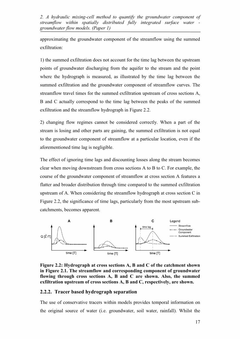
Figure 2.2: Hydrograph at cross sections A, B and C of the catchment shown in Figure 2.1. The streamflow and corresponding component of groundwater flowing through cross sections A, B and C are shown. Also, the summed exfiltration upstream of cross sections A, B and C, respectively, are shown..................................................................... 17
Figure 2.3: The theoretical hydrograph at cross section C of the catchment shown in Figure 2.1. The streamflow, groundwater discharge component and tracer based separation (for dispersivity values of �L1 and �L2) are shown. .......................................................................... 18
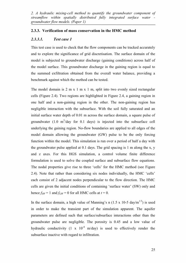
Figure 2.4: Test case 1: “two-region” model grid, and HMC cells for HGS nodes in “two-region” model grid. In the right part of the figure the two nodes at y = 0 belong to HMC cell 1, the two nodes at y = 1 belong to HMC cell 2 and the nodes at y = 3 belong to HMC cell 3. .......... 26
Figure 2.5: HMC cell, SW and GW balances (top panel) and fractions (bottom panel) for test case 1. The volumetric balance in the top row shows the HMC calculated balances for SW and GW in the HMC cells as well as the total volume in the cell which is calculated directly from the model outputs. The HMC cell SW and GW fractions in the bottom panel are calculated independently of each other. ................ 28
Figure 2.6: The 21 HMC cells for the "two-region" model with dy = 10 cm. .... 29
Figure 2.7: Effect of temporal discretisation on the SW and GW fractions in HMC cells 1, 11 and 21. ................................................................... 29
Figure 2.8: Test case 2 catchment model (modified version of the V-catchment in Panday and Huyakorn (2004)). The contours correspond to the elevation. .......................................................................................... 31
Figure 2.9: Part cross section of hypothetical catchment highlighting the raised plane which is used to create a greater hydraulic gradient next to the stream leading to constant subsurface to surface exchange along the

List of Figures
xiv
entire length (from x = 790 – 810 m, at y = 0 m and z = -4 to 2 m). The plane (left), bank (middle) and streambed (right) are seen in the division of top cells. ......................................................................... 32
Figure 2.10: Evolution of the losing section of the stream in the hypothetical catchment. A positive exchange in the top panel of plots denotes subsurface to the surface exchange and vice versa for a negative exchange. The depth and velocity profile along the stream are shown below. At t = 1 second, the stream is gaining along the full length. At b.) t = 12 days, the pumping has reduced the positive exchange section of the stream adjacent to the pumping location. At c.) t = 40 days, the stream is partially losing along a small section whilst maintaining flow along the losing section. ....................................... 35
Figure 2.11: HMC direct rainfall (RF) and groundwater (GW) component fractions before and after the first rainfall event for cells 1, 13, and 21. Note the time lags of rainfall in the downstream cells 13 and 21 (~3.5hrs). .......................................................................................... 37
Figure 2.12: Hyetograph for catchment and Hydrograph at the catchment outlet, showing separation of direct rainfall and groundwater components of streamflow, as well as the summed exfiltration from the overall water balance. The summed exfiltration (SE) from the water balance is clearly seen to exceed the outflow in this hypothetical catchment. The HMC direct rainfall and groundwater components of streamflow are calculated using the HMC fractions in HMC cell 21. ................ 38
Figure 3.1: Modified tilted V-catchment used for simulation of the synthetic catchment’s rainfall response. Points 1 and 2 denote locations of groundwater pumps. Note that due to the symmetry of the catchment, only half of it is shown. .................................................. 51
Figure 3.2: Streamflow hydrograph at the outlet and HMC flow components for scenario 1 (without pumping), with highlighted events. An apparent steady-state baseflow rate was observed in the first event (10.5-11 days) and second event (21.4-23 days). ............................................ 60
Figure 3.3: Streamflow hydrograph at the outlet and HMC flow components for scenario 2 (with pumping), with highlighted events. An apparent steady-state baseflow rate was observed in the first two rainfall events. ............................................................................................... 60
Figure 3.4: Streamflow hydrograph at the outlet and HMC flow components for modified scenario 1 (with 5mm/day ET), with highlighted events. An apparent steady-state baseflow rate was still observed in the first event (10.5-11 days) and second event (21.4-23 days). ................... 61
Figure 3.5: Values of recession constant a and R2 value for the linear regression of Qt vs Qt+1, for sand and initial conditions WT1, WT2, WT3 and without/with pumps 1 and 2 active. The high value of R2 suggests a linear storage-discharge relationship at the outlet during recession periods. ............................................................................................. 62
Figure 3.6: Performance based ranking using BFI over the whole simulation for HYSEP, PART, BFLOW and the Eckhardt separation methods. 1 indicates best performance, 10 indicates worst performance. .......... 69

List of Figures
xv
Figure 3.7: Comparison of simulated daily baseflow and baseflow estimated using HYSEP, PART, BFLOW and the Eckhardt separation methods for scenario 1. ................................................................................... 70
Figure 4.1: Location of the Lehstenbach catchment, after Frei et al. (2010). .... 83
Figure 4.2: Conceptual diagram of in-stream and overland flow generation mechanisms typical of the Lehstenbach catchment during intense storm events. The in-stream and overland flow generation mechanisms shown are groundwater discharge to the channel (GW-CH) and wetland surfaces (GW-WL), direct rainfall to the channel (RF-CH) and wetland surfaces (RF-WL), and runoff from the forest. .......................................................................................................... 84
Figure 4.3: Geometry of the wetland segment: a) planar reference model showing the main drainage direction and channel location; b) smoothed realisation of the wetlands’ hummocky micro-topography, with simulation results of developed overland flow in the wetland (after Frei et al. (2010)); c) cross section (Y = 5 m) of the micro-topography model (after Frei et al. (2010)). The division of overland flow into two distinct flow networks (denoted as FN1 and FN2) is shown by the surface flow lines. The model observation points for flow in this study are denoted by the red arrows, which correspond to surface water discharge from the wetlands to the channel from FN1 and FN2, and channel discharge at the outlet of the model. ............. 86
Figure 4.4: Model spatial discretisation of the Lehstenbach catchment and distribution of the stream, wetland and forest areas (the z-axis is exaggerated by a factor of 5). Model observation points are at locations 1 to 6 and the outlet. .......................................................... 89
Figure 4.5: Hyetograph, simulated outlet hydrograph, simulated FN1 hydrograph, simulated FN2 hydrograph and simulated surface water storage graph for the wetland model during a large storm event. GW-CH and RF-CH are direct groundwater discharge and rainfall to the channel. GW-WL and RF-WL represent groundwater discharge and rainfall to the surface of the wetland area respectively. Initial represents the initial water in the surface domain at the beginning of the simulation. The reset fraction of flow was negligible and hence is not shown. ......................................................................................... 99
Figure 4.6: Wetland HMC fractions at day 14 (pre-storm event). The in-stream and overland flow generating mechanisms shown are: a) groundwater discharge to the channel (GW-CH), b) groundwater discharge to the wetland surface (GW-WL). The initial and reset fractions are also shown in c) and d) respectively. A GW-WL fraction of 0.5 denotes that 50% of the water at that cell was generated from groundwater discharging to the wetland surface. .. 101
Figure 4.7: Wetland HMC fractions at day 20 (during the storm event). In-stream and overland flow generating mechanisms shown are: a) groundwater discharge to the channel, b) groundwater discharge to the wetland surface, c) rainfall to the channel, d) rainfall to the wetland. The remaining initial water (e) and the reset fraction (f) for reset cells are also shown................................................................ 102

List of Figures
xvi
Figure 4.8: Comparison of different streamflow generation mechanism contributions at the outlet, FN1 and FN2. The initial and reset fractions and the cumulative error in the cells were insignificant, as can be seen at the top of the stacked columns. ............................... 103
Figure 4.9: Simulated surface saturation (a), exchange flux (b) and surface water depth (c), prior to the storm, at the storm peak and 2 days after the storm peak. A losing section on the right arm of the stream is highlighted in the third frame of row b). Positive values of exchange flux indicate groundwater discharge to the surface and negative values indicate infiltration of surface water to the subsurface. ...... 104
Figure 4.10: Hyetograph (a), separated discharge hydrographs at the outlet (b), as well as the HMC fractions in surface-storage across the catchment (c). Note that overland flow from the forest was negligible (< 0.2%) in contributing to streamflow and so is not shown in (b). .............. 106
Figure 4.11: HMC calculated in-stream and overland flow generation for the Lehstenbach catchment – before peak (day 216), at peak (day 218) and after the peak (day 220). The flow generation components are: a) groundwater discharge to the channel (GW-CH), b) rainfall to the channel (RF-CH), c) groundwater discharge to the wetlands surfaces (GW-WL), and d) rainfall to the wetlands (RF-WL). The initial fractions are not shown as all initial water has been flushed from the catchment. The reset fractions are shown in row e). ...................... 108
Figure 4.12: Box plots showing the spread of the average in-stream and overland flow generation mechanism contributions for the entire year and during the large storm event, across the 7 different model observation points. The thick black line represents the median; the box covers the inter quartile range (IQR) bounded by the lower and upper quartiles; the whiskers extend to the lowest and highest data point within the fences (where the fences are 1.5 x IQR above and below the upper and lower quartiles respectively); the circles represent data above and below the upper and lower fences respectively. .................................................................................... 110
Figure 4.13: Comparison of active and contributing processes with respect to a) GW-CH, b) RF-CH, and c) WL-CH (where WL-CH = RF-WL + GW-WL). Note that the contributing component is superimposed on top of the active component in each of these graphs, i.e. they are not stacked. The long-term ratio of contributing to active processes is also noted in each of the plots, which highlights the average difference between the two. The dashed and dotted lines on each plot represent respectively the cumulative active and contributing components. .................................................................................... 112
Figure 5.1: Comprehensive conceptualisation of catchment response to rainfall (adapted from Sklash and Farvolden, 1979). The dashed red line indicates the aspects considered in this research, although without distinction of overland rainfall driven mechanisms (i.e. infiltration excess (Hortonian) or saturation excess (Dunne)). ......................... 124
List of Tables
xvii
List of Tables Table 2.1: Maximum relative error in the HMC method, and the global volume
error (GVE) for the HMC method. ..................................................... 30
Table 2.2: Surface and subsurface parameters for test case 2. ............................. 33
Table 3.1: Surface and subsurface parameters for the synthetic catchment model. For a detailed description of these model parameters see Therrien et al. (2009). ............................................................................................ 52
Table 3.2: Scenarios for simulating catchment response. Scenarios with an asterisk denote scenarios where groundwater pumping is applied in the catchment. ..................................................................................... 56
Table 3.3: BFI, NSE and PBIAS for simulated baseflow and estimated baseflow during event 1 using HYSEP, PART, BFLOW and the Eckhardt separation methods. Lightly shaded cells highlight a NSE < 0.5 and darkly shaded cells highlight │PBIAS│ > 25%. Scenarios with an asterisk denote where groundwater pumping is applied in the catchment. ........................................................................................... 65
Table 3.4: BFI, NSE and PBIAS for simulated baseflow and estimated baseflow during event 2 using HYSEP, PART, BFLOW and the Eckhardt separation methods. Lightly shaded cells highlight a NSE < 0.5 and darkly shaded cells highlight │PBIAS│ > 25%. Scenarios with an asterisk denote where groundwater pumping is applied in the catchment. ........................................................................................... 66
Table 3.5: BFI, NSE and PBIAS for simulated baseflow and estimated baseflow during event 3 using HYSEP, PART, BFLOW and the Eckhardt separation methods. Lightly shaded cells highlight a NSE < 0.5 and darkly shaded cells highlight │PBIAS│ > 25%. Scenarios with an asterisk denote where groundwater pumping is applied in the catchment. ........................................................................................... 67
Table 3.6: Comparison of BFI, NSE and PBIAS for (scenario 1 with and without ET) simulated baseflow and estimated baseflow during event 2 using HYSEP, PART, BFLOW and the Eckhardt separation methods. Lightly shaded cells highlight a NSE < 0.5 and darkly shaded cells highlight │PBIAS│ > 25%. ................................................................ 68
Table 4.1: Surface and subsurface parameters used in the Lehstenbach catchment model. For a detailed description of all model parameters used in HGS, see Therrien et al. (2009). ......................................................... 90
Table 4.2: Considered flow generation mechanisms, HMC unique fractions, and HMC fraction types. ............................................................................ 97

xviii

1. Introduction
1
Chapter 1
1 Introduction The understanding of hydrological processes and their translation to the
streamflow hydrograph is critical in the management of floods and water
resources, and the environments they support. A key to this is the understanding
of the interactions of surface and subsurface water systems within catchments
(Winter, 1999; Sophocleous, 2002). The important feedbacks exhibited by these
two systems, necessitate their holistic consideration within catchment hydrology.
Therefore, improving this understanding requires both the identification and
quantification of surface-subsurface water interactions (e.g. losing streams) and
flow generation/depletion processes (e.g. rainfall-runoff and dry-period baseflow).
This means having a clear understanding of the physics of water movement within
catchments. If the physics understanding is clear, and the system is well
characterised, then it follows that the integrated catchment response – in the form
of the streamflow hydrograph – should be able to be readily decomposed into the
constituent flow generation processes, i.e. groundwater discharge and direct
rainfall to the stream, and groundwater discharge and direct rainfall to the
hillslope (see Figure 1.1).
It was highlighted by Hewlett and Troendle (1975) that accurate prediction of the
streamflow hydrograph implies adequate modelling of the sources, flowpaths and
residence time of water. This “adequate” modelling suggests the use of spatially
and temporally distributed hydrological models, of which many have been
developed (see Singh and Woolhiser (2002) for a comprehensive review). It
follows from Hewlett and Troendle’s statement that adequate modelling of the
sources, flowpaths and residence times requires adequate representation of the
physics of water flow, i.e. deterministic-conceptual modelling (see Kampf and
Burges, 2007).

1. Introduction
2
Figure 1.1: Streamflow generation at the plot scale by both in-stream (groundwater discharge and rainfall to the stream channel) and overland (groundwater discharge and rainfall to the hillslope) flow generation processes.
Freeze and Harlan (1969) provided a blueprint for what is often considered
“adequate” physics-based modelling of water flow within catchments. The
inevitably complex models that arise from this blueprint can aid in building
intuition about the catchment-scale hydrological processes responsible for
streamflow, but subject to the assumptions in the physical equations (e.g. that a
representative elementary volume exists in the subsurface).
In the last decade, the blueprint of Freeze and Harlan (1969) has been realised
with the advent of physics-based fully Integrated Surface-Subsurface
Hydrological Models (ISSHM) (Gaukroger and Werner, 2011). Examples of
ISSHMs include InHM (VanderKwaak and Loague, 2001), MODHMS
(HydroGeoLogic, 2006), HydroGeoSphere (HGS) (Therrien et al., 2009), and
ParFlow (Kollet and Maxwell, 2006). ISSHMs are used within this thesis to
describe models which solve simultaneously the surface and subsurface flow
equations. Within ISSHMs, 2D surface flow is usually represented using an
approximation to the St Venant equations (e.g. diffusion wave), and 3D variably
saturated subsurface flow is usually represented using Richard’s equation.
ISSHMs can be used to analyse and interpret hydrological processes and in
developing conceptual understanding of catchment processes (Ebel and Loague,
2006). A particularly important attribute of these models is that rainfall is
partitioned into infiltration, ponding, and overland flow in a realistic manner

1. Introduction
3
(Therrien et al., 2009) without any a priori assumption of these processes (Mirus
et al., 2011a). This partitioning is dependent on the rate of rainfall, antecedent
moisture conditions and catchment physical characteristics. However, this means
that the hydrological processes (e.g. groundwater discharge to a stream or
infiltration excess overland flow) need to be identified and interpreted after
simulations.
Studies utilising ISSHMs are becoming increasingly widespread (e.g., Frei et al.,
2010; Maxwell and Kollet, 2008; Park et al., 2011; Brunner et al., 2009). These
examples focused on processes in small-scale synthetic systems, which enabled
insight to be gained into the controls on flow generation (Frei et al., 2010;
Maxwell and Kollet, 2008; Park et al., 2011) and depletion (Brunner et al., 2009).
In larger-scale (e.g. catchment scale) systems it is difficult to resolve how the
hydrological drivers affect the hydrological outputs (e.g. the outlet streamflow
hydrograph). This is because hydrological outputs at a given point in space and
time are only affected by hydrological drivers that occur at the same location and
at the same time (i.e. by ‘active’ processes (Ambroise, 2004)). In larger-scale
systems, hydrological drivers that occur at a particular point in time (active
processes) do not necessarily end up contributing to the hydrological output at that
or a later time. This is because of the influence of travel times, flow impediments
(e.g. riparian wetlands or weirs), and losses (e.g. infiltration or evaporation).
Consequently, where such influences are significant, there is a need to distinguish
between ‘active’ and ‘contributing’ streamflow generation processes (Ambroise,
2004), where contributing processes are those that contribute to flow at a
particular location at a particular time, and potentially include active processes.
These influences will be important in catchments that exhibit significant travel
times for water and/or where flow depletion processes are significant relative to
flow generation processes (e.g. strong losing streams). The differences between
active and contributing flow generation processes are driven by active flow
depletion mechanisms (surface water losses) and the lag-time between active flow
generation mechanisms taking place and the time that the resultant flow reaches
the point of interest (e.g. the point where the streamflow hydrograph is measured).
A key shortcoming of ISSHMs is in linking the distributed hydrologic response to
the point response (e.g. where the streamflow hydrograph is measured), i.e.

1. Introduction
4
capturing the contributing processes. Active processes are readily obtained from
ISSHMs that output the nodal fluid mass balance components, i.e. surface-
subsurface exchange fluxes, rainfall input, evaporation output, surface inflows and
outflow and changes in storage. However, attaining the contributing processes
requires the ability to use these outputs of active processes to properly analyse and
interpret streamflow generation mechanisms with respect to the streamflow
hydrograph.
The advent of ISSHMs has been critical in being able to improve our conceptual
understanding of hydrological processes, but the benefits of analysing internal
processes and meaningfully separating flow hydrographs are still to be realised.
This is a major shortcoming as it prevents development in building the intuition of
hydrologic response to various hydrological drivers (i.e. rainfall and
evapotranspiration). A clear need has arisen for research into the identification
and quantification of contributing in-stream and overland flow generation
mechanisms at larger (e.g. catchment) scales, particularly given that there are still
difficulties in the ability to conduct or scale up the measurements that are required
in order to gain this understanding at/to the catchment scale (Fleckenstein et al.,
2010).
1.1. Research Objectives
This research aims to improve the understanding of streamflow generation and
surface water-groundwater interaction through quantifying in-stream and overland
flow generation mechanisms within physics-based models of surface-subsurface
flow. In such models, this requires the development of a new method for
interpreting in-stream and overland flow generation mechanisms. This
development will provide a platform for investigation into hydrological systems
that exhibit complex spatiotemporal patterns of in-stream and overland flow
generation mechanisms. To achieve the overall aims of this research, four main
research objectives are developed with three sub-objectives, which are listed
below. The linking of each of these objectives is shown in Figure 1.2.
Objective 1: To develop a method to quantify the contribution of flow generation
mechanisms to streamflow, allowing separation of the streamflow hydrograph into
its constituent flow generation components (i.e. groundwater discharge and direct
1. Introduction
5
rainfall to the stream, and groundwater discharge and direct rainfall to overland
areas).
Objective 1.1: To improve model based investigation into groundwater
discharge to total streamflow within streams exhibiting complex stream-
aquifer interactions.
Objective 1.2: To improve model-based investigation into the contribution
to total streamflow of rainfall and groundwater discharge from overland
areas.
Objective 2: To develop a benchmark against which baseflow separation methods
can be tested against.
Objective 2.1: To determine the potential error in commonly used
automated methods for estimation of in-stream groundwater contributions
to streamflow.
Objective 3: To investigate the spatiotemporal variability in both overland and in-
stream flow generation mechanisms within a modelling framework.
Objective 4: To investigate the dichotomy that exists between ‘active’ and
‘contributing’ streamflow generation mechanisms within a modelling framework.
Objective 5: To incorporate the method developed in Objective 1 into an ISSHM
code to provide a platform for other researchers to utilise the method developed
within this research.

1. Introduction
6
Figure 1.2: Research objectives and their hierarchy. Objectives are denoted by the superscript numbers in each of the flowchart boxes.
1.2. Thesis Overview
This thesis is organised into five chapters. The main body of this thesis consists of
Chapters 2 to 4, which correspond to three journal papers (Partington et al.,
2011; Partington et al., 2012a; Partington et al., 2012b). In Chapter 2
(Partington et al., 2011) a new method is developed for accurately quantifying
groundwater contributions to streamflow (Objective 1) with respect to the
streamflow hydrograph, and this method is used to investigate the complexity of
groundwater contributions to streamflow (Objective 1.1). In Chapter 3
(Partington et al., 2012a) the work in Chapter 2 is extended, and a baseflow
model benchmark is developed (Objective 2) against which potential error is
investigated in commonly used automated methods for the separation of baseflow
from streamflow hydrographs (Objective 2.1). In Chapter 4 (Partington et al.,
2012b) the work of Chapter 2 is extended to investigate overland flow generation
mechanisms (Objective 1.2), and the new method is applied to a case study of a
real catchment. Within the case study, all surface flow generation mechanisms are
quantified (Objective 1.2), spatiotemporal variability in flow generation
mechanisms is analysed (Objective 3), and the difference between active and
Quantifying flow generation mechanisms1
In-stream flow generation mechanisms1.1, 1.2
Overland flow generation mechanisms1.2
Groundwater discharge to stream1.1 ,1.2
Direct rainfall on
stream1.1, 1.2
Overland flow to
stream1.2, 2
Baseflow benchmark2
Groundwater discharge to overland1.2
Direct rainfall on overland1.2
Streamflow to
overland1.2
Testing automated baseflow separation
methods2.2
Separated Hydrographs1 Spatiotemporal
Analysis3 Active vs.
Contributing4
Development of method to quantify streamflow generation mechanisms1
Implementation of method within an ISSHM5

1. Introduction
7
contributing processes is analysed (Objective 4). The linking of each of the
papers to the objectives is depicted below in Figure 1.3. Although the manuscript
has been reformatted in accordance with University guidelines, and sections
renumbered for inclusion within this thesis, the material within this paper is
otherwise presented herein as published. Copies of the publications “as published”
are provided in the Appendix A and B.
Figure 1.3: Linkage of research objectives and publications.
Conclusions of the research within this thesis are provided in Chapter 5, which
summarises: 1) the research contributions, 2) limitations and 3) future directions
for further research.
Quantifying flow generation mechanisms1
In-stream flow generation mechanisms1.1, 1.2
Overland flow generation mechanisms1.2
Groundwater discharge to stream1.1 ,1.2
Direct rainfall on
stream1.1, 1.2
Overland flow to
stream1.2, 2
Baseflow benchmark2
Groundwater discharge to overland1.2
Direct rainfall on overland1.2
Streamflow to
overland1.2
Testing automated baseflow separation
methods2.2
Separated Hydrographs1 Spatiotemporal
Analysis3 Active vs.
Contributing4
Development of method to quantify streamflow generation mechanisms1
Paper 1
Paper 2
Paper 3
Implementation of method within an ISSHM5

8

9
Chapter 2
2 A hydraulic mixing-cell method to quantify the groundwater component of streamflow within spatially distributed fully integrated surface water - groundwater flow models (Paper 1)

10

11
Publication Details
This work has been published within the journal Environmental Modelling and
Software as the following article:
Partington, D., P. Brunner, C. T. Simmons, R. Therrien, A. D. Werner, G.
C. Dandy, and H. R. Maier. 2011. A hydraulic mixing-cell method to
quantify the groundwater component of streamflow within spatially
distributed fully integrated surface water - groundwater flow models.
Environmental Modelling and Software, 26:886-898.
Although the manuscript has been reformatted in accordance with University
guidelines, and sections renumbered for inclusion within this thesis, the material
within this paper is otherwise presented herein as published.
Statement of Authorship
Partington, D. (Candidate)
Development of HMC method, testing and implementation of method, wrote
manuscript.
Signed: . . . . . . . . . . . . . . . . . . . . . . . . . . . . . . . . . . . . . . . . . . . . . . . . Date: . . . . . . .
Brunner, P.
Supervised manuscript preparation and reviewed draft
Signed: . . . . . . . . . . . . . . . . . . . . . . . . . . . . . . . . Date: . . . . . . .
Simmons, C.T.
Supervised manuscript preparation and reviewed draft
Signed: . . . . . . . . . . . . . . . . . . . . . . . . . . . . . . . . . . . . . . . . . . . . . . . . Date: . . . . . . .
Therrien, R.
Supervised manuscri draft
Signed: . . . . . . . . . . . . . . . . . . . . . . . . . . . . . . . . . . . . . . . . . . . . . . . . Date: . . . . . . .
Werner, A.D.
Supervised manuscript preparation and reviewed draft
Signed: . . . . . . . . . . . . . . . . . . . . . . . . . . . . . Date: . . . . . . .

12
Maier, H. R.
Supervised manuscript preparation and reviewed draft
Signed: . . . . . . . . . . . . . . . . . . . . . . . . . . . . . . . . . . . . . . . . . . . . . . . . Date: . . . . . . .
Dandy, G. C.
Supervised manuscrip
Signed: . . . . . . . . . . . . . . . . . . . . . . . . . . . . . . . . . . . . . . . . . . . . . . . . Date: . . . . . . .

2. A hydraulic mixing-cell method to quantify the groundwater component of streamflow within spatially distributed fully integrated surface water - groundwater flow models. (Paper 1)
13
Abstract
The complexity of available hydrological models continues to increase, with fully
integrated surface water-groundwater flow and transport models now available.
Nevertheless, an accurate quantification of streamflow generation mechanisms
within these models is not yet possible. For example, such models do not report
the groundwater component of streamflow at a particular point along the stream.
Instead, the groundwater component of streamflow is approximated either from
tracer transport simulations or by the sum of exchange fluxes between the surface
and the subsurface along the river. In this study, a hydraulic mixing-cell (HMC)
method is developed and tested that allows to accurately determine the
groundwater component of streamflow by using only the flow solution from fully
integrated surface water - groundwater flow models. By using the HMC method,
the groundwater component of streamflow can be extracted accurately at any
point along a stream provided the subsurface/surface exchanges along the stream
are calculated by the model. A key advantage of the HMC method is that only
hydraulic information is used, thus the simulation of tracer transport is not
required. Two numerical experiments are presented, the first to test the HMC
method and the second to demonstrate that it quantifies the groundwater
component of streamflow accurately.
2.1. Introduction
A quantitative understanding of stream flow hydrographs is an important
precondition to the understanding and effective management of any catchment
(VanderKwaak and Loague, 2001; Jones et al., 2006; Mirus et al., 2009). The
streamflow hydrograph is generated by different mechanisms such as groundwater
discharge to the stream, discharge from the unsaturated zone, overland flow,
preferential flow through macropores and/or fractures, and direct precipitation to
the stream. These streamflow generation components can exhibit complex spatial
and temporal behaviour. This complexity makes it difficult to easily decompose
stream flow hydrographs in terms of stream flow generation mechanisms if one or
several components of the hydrograph are unknown. Groundwater discharge is a
critical streamflow generation component that is difficult to quantify. The
quantitative assessment of the groundwater component of streamflow (which

2. A hydraulic mixing-cell method to quantify the groundwater component of streamflow within spatially distributed fully integrated surface water - groundwater flow models. (Paper 1)
14
represents the quantity of streamflow at a given point in space and time consisting
of groundwater discharging directly to the stream) is of great importance in
understanding catchment hydrology and informing water resources management,
as highlighted by Sophocleous (2002) and Winter (1999). Accurate simulation of
the groundwater component of streamflow is therefore important in hydrological
modelling exercises (e.g. Gilfedder et al., 2009; Croton and Barry, 2001; Facchi
et al., 2004) in order to inform water resources management.
The groundwater component of stream flow cannot be measured easily in the field
(Hatterman et al., 2004) and therefore is usually quantified using indirect
methods. Indirect methods can involve the use of environmental and conservative
tracers for separation of the hydrograph (McGlynn and McDonnell, 2003;
McGuire and McDonnell, 2006), and recession analysis based on conceptual
storage-discharge relationships for the catchment (Chapman, 2003; Eckhardt,
2008). However, as pointed out by Hewlett and Troendle (1975), ‘the accurate
prediction of the hydrograph implies adequate modelling of the sources, flowpaths
and residence time of water’. In particular, capturing the flowpaths requires a
spatially distributed model. Unless the assumptions of the indirect methods can be
resolved or justified, the adequate modelling of sources and flowpaths of water
would be insufficient. If the modelling is insufficient, then it follows that the
separation of the hydrograph may be meaningless. Given the difficulty faced in
accurately measuring sources and flowpaths within hillslopes, let alone entire
catchments, some benefit can be found in examining hypotheses which can be
adequately ‘measured’ in the ‘virtual laboratory’ (Weiler and McDonnell, 2006).
One could expect that the tools for quantifying the groundwater component of
streamflow are now readily available in the latest generation of fully integrated
spatially distributed models such as InHM (VanderKwaak and Loague, 2001),
MODHMS (HydroGeoLogic, 2006), HydroGeoSphere (HGS) (Therrien et al.,
2009), Wash123D (Cheng et al., 2005) and ParFlow (Kollet and Maxwell, 2006).
However, this is not the case. Even within spatially distributed numerical models
quantifying source components remains a challenge (Sayama and McDonnell,
2009). The same applies to the ultimate delivery mechanisms as defined in Sklash
and Farvolden (1979). Because the currently available numerical models do not

2. A hydraulic mixing-cell method to quantify the groundwater component of streamflow within spatially distributed fully integrated surface water - groundwater flow models. (Paper 1)
15
report the groundwater component of streamflow at a given location, it is often
approximated by introducing tracers or by setting it equal to the summed
exfiltration along a section or entire length of the stream. The summed exfiltration
is defined in this paper as the sum of all fluxes from the subsurface to the stream
at a specific point in time upstream of the point at which the hydrograph is
measured.
However, these approaches are problematic. For example, the summed exfiltration
during a simulation is not equal to the groundwater component of streamflow at
the same simulation time. This can be attributed to the fact that portions of the
summed exfiltration exhibit a time lag from the point of entering the stream to the
point of streamflow measurement, as a result of potentially significant transit
times within stream networks (McGuire and McDonnell, 2006). This time lag
cannot be captured if the groundwater component of streamflow is approximated
by the summed exfiltration. Furthermore, if the stream loses water to the
subsurface between a point of groundwater discharging into the stream and the
point where the hydrograph is measured, only a portion of the groundwater
entering the stream will contribute to the groundwater component of streamflow
at the point of hydrograph measurement. In that case, the summed exfiltration will
overestimate the groundwater component of streamflow at the point of
hydrograph measurement.
In this study, a mixing-cell method for quantifying the groundwater component of
streamflow in fully integrated spatially distributed models is described. Mixing-
cell models have often been used in hydrogeology to model solute transport (Adar
et al., 1988; Campana and Simpson, 1984). Mixing-cell models rely only on
conservation of mass. The hydraulic mixing-cell (HMC) method described in this
study relies on hydraulic information only (i.e. fluxes). Moreover, the method
allows tracking streamflow generation mechanisms at every cell or element within
the stream of the model domain. Therefore, complex spatial and temporal effects
are captured and can be accounted for. The method is developed and tested using
a particular numerical model (HydroGeoShpere, Therrien et al., 2009), but it can
be implemented to any code that reports the exchange between the subsurface and
surface in a spatially distributed manner. The paper also aims to explore the

2. A hydraulic mixing-cell method to quantify the groundwater component of streamflow within spatially distributed fully integrated surface water - groundwater flow models. (Paper 1)
16
suitability of traditional methods (e.g. equilibrating the groundwater component of
streamflow to the summed exfiltration) for quantifying the groundwater
component of streamflow within numerical models.
2.2. Existing methods for extracting streamflow generation components
The hypothetical catchment shown in Figure 2.1 is used to illustrate the
challenges of extracting the groundwater component of streamflow from
numerical models using existing methods. In the catchment shown, the stream,
which is flowing from A to B to C, is gaining in sections A and C, but losing in
section B.
Figure 2.1: Conceptual diagram of a surface water-groundwater catchment (left hand side) featuring different flow regimes (as illustrated in the right part of the figure). The white sections of the catchment adjacent to the stream represent the groundwater discharge upslope of the stream (return flow). The dashed lines on the right part of the figure represent the water table. The flow direction is towards the reader.
2.2.1. Summed exfiltration along the length of the stream
For each of cross sections A, B and C of the hypothetical catchment shown in
Figure 2.1, the expected streamflow hydrograph is shown in Figure 2.2, along
with the groundwater component of streamflow and the summed exfiltration. The
streamflow in Figure 2.2 A, B and C refers to the point measurement at each of
cross sections A, B and C. Although the results shown in Figure 2.2 are
hypothetical, they illustrate the following two problems that arise by
2. A hydraulic mixing-cell method to quantify the groundwater component of streamflow within spatially distributed fully integrated surface water - groundwater flow models. (Paper 1)
17
approximating the groundwater component of the streamflow using the summed
exfiltration:
1) the summed exfiltration does not account for the time lag between the upstream
points of groundwater discharging from the aquifer to the stream and the point
where the hydrograph is measured, as illustrated by the time lag between the
summed exfiltration and the groundwater component of streamflow curves. The
streamflow travel times for the summed exfiltration upstream of cross sections A,
B and C actually correspond to the time lag between the peaks of the summed
exfiltration and the streamflow hydrograph in Figure 2.2.
2) changing flow regimes cannot be considered correctly. When a part of the
stream is losing and other parts are gaining, the summed exfiltration is not equal
to the groundwater component of streamflow at a particular location, even if the
aforementioned time lag is negligible.
The effect of ignoring time lags and discounting losses along the stream becomes
clear when moving downstream from cross sections A to B to C. For example, the
course of the groundwater component of streamflow at cross section A features a
flatter and broader distribution through time compared to the summed exfiltration
upstream of A. When considering the streamflow hydrograph at cross section C in
Figure 2.2, the significance of time lags, particularly from the most upstream sub-
catchments, becomes apparent.
Figure 2.2: Hydrograph at cross sections A, B and C of the catchment shown in Figure 2.1. The streamflow and corresponding component of groundwater flowing through cross sections A, B and C are shown. Also, the summed exfiltration upstream of cross sections A, B and C, respectively, are shown.
2.2.2. Tracer based hydrograph separation
The use of conservative tracers within models provides temporal information on
the original source of water (i.e. groundwater, soil water, rainfall). Whilst the

2. A hydraulic mixing-cell method to quantify the groundwater component of streamflow within spatially distributed fully integrated surface water - groundwater flow models. (Paper 1)
18
application of solutes is extremely useful in identifying the source of streamflow,
it gives no real indication of the mechanism of streamflow generation (McGuire
and McDonnell, 2006). Even with temporal information on the source of water,
the parameters associated with tracer transport (i.e. diffusion, tortuosity and
dispersivity) often affect the interpretation of the source as demonstrated in Jones
et al. (2006). Jones et al. (2006) found that the value of dispersivity used in
simulating the transport of tracers could lead to large overestimation of the pre-
event water’s contribution to streamflow. In their model using InHM of the
Borden rainfall-runoff experiment, the pre-event contributions to streamflow
using longitudinal dispersion �L = 0.5 m and 0.005 m were found to be 41.6% and
33.9%, respectively, with the hydraulically based subsurface contribution close to
0%. These results would suggest that in the streamflow hydrograph in Figure 2.1
at cross section C of the catchment, the groundwater component of streamflow
could be easily overestimated using tracers as illustrated in Figure 2.3.
Figure 2.3: The theoretical hydrograph at cross section C of the catchment shown in Figure 2.1. The streamflow, groundwater discharge component and tracer based separation (for dispersivity values of �L1 and �L2) are shown.
Given such large variation in the tracer based interpretations of groundwater
contributions to streamflow, it seems quite clear that inherent accuracy relies on
reliability and certainty of the transport parameters. Any uncertainty in the
dispersivity directly relates to uncertainty in quantifying the groundwater
component of streamflow. Therefore quantifying the groundwater component of
the streamflow hydrograph within models using tracers may be undermined by
large uncertainty.

2. A hydraulic mixing-cell method to quantify the groundwater component of streamflow within spatially distributed fully integrated surface water - groundwater flow models. (Paper 1)
19
2.3. A hydraulic balance using a hydraulic mixing-cell method
The hydraulic mixing-cell (HMC) method introduced in this paper allows the
streamflow generation mechanisms to be deconvoluted from the streamflow
hydrograph at any point along the stream. The method relies on standard
hydraulic output from numerical models only. It is based on the modified mixing
cell of Campana and Simpson (1984). Furthermore, it is assumed for the
simplicity of coding that the width of the stream does not change during the
simulation and additionally that the flow direction in the stream does not change.
This mass balance of the HMC method is verified by application to two numerical
test cases using HydroGeoSphere. The method can be generalised to any spatially
distributed surface water - groundwater code, as mentioned previously.
2.3.1. Theory
The numerical modelling of streamflow requires discretisation over space and
time of the relevant governing flow equation using a finite difference (FD), finite
volume (FV) or finite element (FE) scheme. The method developed herein is
designed to fit in accordingly with existing numerical models.
Consider the continuity of flow for a stream cell i of arbitrary shape. This can be
expressed in terms of the streamflow generation/depletion as:
dtdVQQQQQQQQ EvapDownRainPFUFOFGWUp ��������
(2.1)
Where QUp [L3/T] is the upstream flow (generated from groundwater, overland
flow, unsaturated flow and rainfall) into the stream cell; QGW, QOF, QUF and QPF
[L3/T] are the groundwater, overland flow, unsaturated flow and preferential flow,
respectively, flowing into or out of the cell; QRain [L3/T] is the rainfall contribution
to the stream cell, QDown is the flow downstream (generated from groundwater,
overland flow, unsaturated flow and rainfall) flowing out of the cell [L3/T]; QEvap
[L3/T] is the loss of water from storage (composed of groundwater, overland flow,
unsaturated flow and rainfall) due to evaporation; dV/dt [L3/T] is the rate of
change of storage within the cell.

2. A hydraulic mixing-cell method to quantify the groundwater component of streamflow within spatially distributed fully integrated surface water - groundwater flow models. (Paper 1)
20
More concisely the fluid mass balance for a particular cell i with neighbouring
cells j in the surface domain can be written as:
dt
dVQQ im
jij
n
jji ����
�� 11 (2.2)
Where Qji [L3/T] is the jth flux into the cell i; Qij [L3/T] is the jth flux out of the cell
i; Vi [L3] is the volume in cell i; t [T] is time; and n and m denote n sources and m
sinks.
By multiplying Eq. 2.2 by dt and integrating both sides over the interval t1 to t2,
(t2>t1) we obtain the following:
� �� ���
��� 2
1
2
112
11
t
t
m
jij
t
t
n
jjitt dtQdtQVV
(2.3)
2
1
2
1
1211
t
t
m
jij
t
t
n
jjitt VVVV ��
��
���
(2.4)
For each cell the discrete volumetric balance over each time step dt can be
written:
��
�K
k
Nki
Ni VV
1)( (2.5)
for K streamflow components, where ViN [L3] is the total volume of water in cell i
at time N; Vi(k)N [L3] are the volumes of groundwater flow, unsaturated flow,
overland flow, preferential flow and direct rainfall water, respectively, in cell i at
time N. These constituent balances are defined as:
���
��
�
� ���m
j
N
Nkij
n
j
N
NkjiNki
Nki VVVV
11)(
11)(
1)()(
(2.6)
Where Vji(k) and Vij(k) [L3] are the volumes of the kth component of streamflow
generation into and out of cell i from neighbouring cell j, from time N-1 to N
respectively.

2. A hydraulic mixing-cell method to quantify the groundwater component of streamflow within spatially distributed fully integrated surface water - groundwater flow models. (Paper 1)
21
In order to calculate the volumetric balance, initial conditions of each streamflow
component of the stream water must be known in each cell. The components of
flow are defined as a fraction of the total volume (Vi) such that:
11)(
1)( ���
� �
�N
i
K
k
NkiK
k
Nki V
Vf
(2.7)
Where fi(k)N [L3/L3] is defined as the kth fraction of each streamflow component.
If the form of the function of fluxes can be reconstructed from the flow solution
then, using the modified mixing cell approach of Campana and Simpson (1984),
each component of streamflow can be determined by substituting Eq. 2.6 into Eq.
2.7 and rearranging giving:
Ni
K
k
m
j
N
Nkij
n
j
N
NkjiNkiK
k
Nki V
VVVf
� ��� � �
��
�
�
�
���
���
� 1 11)(
11)(
1)(
1)(
(2.8)
Considering only the kth fraction and expanding out the volumetric terms to
explicitly represent the fractions, then rearranging yields:
Ni
Nkj
n
j
N
NjiNkiN
i
m
j
N
Nij
Ni
NiN
ki V
fVf
V
V
VVf
1)(
11
1)(
111
)(
�
��
���� ��
�
�
�����
�
��
(2.9)
Where there are n sources and m sinks for cell i; fj(k)N-1 denotes fraction k at time
N-1 in neighbouring cell j. The terms on the right hand side of Eq. 2.9 relate to the
stability of this approach. They can be considered from left to right as a.) the ratio
of storage in the previous timestep to the current storage less the ratio of outflow
volume to storage and b.) the ratio of inflow volume to storage. The stability of
this method requires that the volume of water entering or leaving the stream cell
over a time step is not greater than the storage at the end of the time step. This is
fairly intuitive as it is not possible to remove more mass than existed at the start of
the timestep (N-1) or insert more mass than exists at the end of the timestep (N).

2. A hydraulic mixing-cell method to quantify the groundwater component of streamflow within spatially distributed fully integrated surface water - groundwater flow models. (Paper 1)
22
For each component of streamflow the fraction is determined using the modified
mixing cell which approaches a perfectly mixed cell as the time step approaches
zero. A perfectly mixed cell will completely mix all contents across the entire cell
instantaneously and takes the form:
Ni
Nkj
n
j
N
Nji
n
j
N
NjiN
i
Nkj
n
j
N
NjiNki
m
j
N
NijNkiN
i
NiN
ki V
fV
VV
fVfVf
VVf
1)(
11
11
1)(
11
1)(
11
1)(
1
)(
�
��
��
�
��
�
��
�� �
�
���
�
���
��
��
(2.10)
It can be readily seen that Eq. 2.9 approaches Eq. 2.10 as the time step approaches
zero, as only the first term on the right hand side in both equations will remain.
In applying this method, volumes in and out need to be determined at the start and
end of each timestep. This requires reconstruction of the functions describing flux
in and out of each cell. The approach used in calculating volumes needs to be
consistent with the manner in which the fluid mass balance is calculated in the
particular model used. In this study, the HydroGeoSphere (HGS) (Therrien et al.,
2009) code is used in which the flux Q between two adjacent nodes is back
calculated at the end of the time step, giving rise to the following equation for
evaluating the volume in or out over each time step:
)(where 1������� NNNNNij
Nij ttttQV (2.11)
Where QijN denotes the calculated flux from HGS from node i to j over �t.
The form of Eq. 2.11 will vary from code to code depending on how the fluid
mass balance is calculated. Furthermore, the choice of numerical approach, be it
finite difference, finite volume or finite element, is irrelevant as long as the
volumetric balance for each cell is formulated correctly and is mass conservative.
The latter requirement is due to the error in the mass balance at each time step
being cumulative in the HMC method. Stability of the HMC method is not
guaranteed for any flow solution as highlighted above. The use of suitable
convergence criteria within the flow solution is imperative in successful
application of the HMC method. A strict convergence criterion that is applied at

2. A hydraulic mixing-cell method to quantify the groundwater component of streamflow within spatially distributed fully integrated surface water - groundwater flow models. (Paper 1)
23
the nodal level is required. The nodal flow check tolerance in HGS, which is
derived in McLaren et al. (2000), was utilised to ensure the nodal volumetric
balances calculated in the HMC method were sufficient in preventing large
cumulative errors. The choice of timestep and cell size also plays an important
role in the stability of the HMC method because the volumetric balance at each
HMC cell over each timestep is directly related to timestep and cell size. The
proportion of volumes of water entering or leaving each cell over each time step
compared to the storage volume in the cell has a direct impact on the HMC
method’s stability. The use of small HMC cells and large timesteps can lead to the
volume entering or leaving a cell being greater than the storage and as such the
method will become unstable causing spurious oscillations. Hence it is necessary
to use suitable time steps for a fixed grid (i.e. fixed cell size) to ensure stability.
2.3.2. Implementation of the HMC method in HydroGeoSphere
The testing of the HMC method outlined in this paper was carried out by
considering two conceptual test cases using the HGS model. HGS solves the
diffusion wave approximation to the 2D St Venant equations in the surface
domain and solves a modified form of the 3D Richards equation for variably
saturated flow in the subsurface domain using a control volume finite element
approach (details of the model can be found in Therrien et al. (2009)). The surface
and subsurface are coupled using either continuity of head or (as in this study) a
conductance concept, with exchanges between the two domains given by:
)( pmoexch
zzrexch hh
lKkq ��
(2.12)
Where qexch [L/T] is the exchange flux between the surface and subsurface
domain; kr [dimensionless] is the relative permeability; Kzz [L/T] is the saturated
hydraulic conductivity of the porous medium; lexch [L] is the coupling length, ho
[L] and hpm [L] are the heads of the surface and subsurface, respectively. HGS has
been verified for both gaining (Therrien et al., 2009) and losing streams (Brunner
et al., 2009a, 2009b). The model solves the governing flow equations using the
finite element (FE) method, finite volume (FV) method or, alternatively, the finite
difference (FD) method applied on a node centred grid (Therrien et al., 2009).

2. A hydraulic mixing-cell method to quantify the groundwater component of streamflow within spatially distributed fully integrated surface water - groundwater flow models. (Paper 1)
24
Application of the HMC method requires specific HGS model outputs in order to
accurately construct the volumetric balances in each HMC cell. As HGS utilises a
node centred approach, the following HGS outputs are required for the volumetric
balance at any given node:
1.) Computed surface water depth at the node – for the storage at each time step.
2.) Contributing area, CA [L2] for the node determined from finite element basis
functions (1/4 of the area of each element adjacent to the node for both FD and FE
on a structured rectangular grid) – for the Storage ( = depth x CA) [L3] at each
time step.
3.) Exchange flux between the subsurface and surface node – for the volume (Eq.
2.11) exchanged between the subsurface and surface over each time step.
4.) Flux from upstream contributing nodes – for the upstream volume (Eq. 2.11).
5.) Flux to downstream nodes – for the downstream volume (Eq. 2.11).
1.) and 2.) are used to calculate Vi, 3.) used to calculate Vji for the exchange, 4.)
used to calculate Vji for upstream flow, 5.) used to calculate Vij for downstream
flow. The initial values for the fractions of stream flow are subjective and so a
dummy (or undefined) fraction can be used until the streamwater is turned over at
which point the dummy fraction will be zero.
This output data provides all the information required to apply the HMC method
and determine the groundwater component of streamflow at each time step in each
cell of the stream. The partitioning of groundwater, overland flow and rainfall
entering the HMC cell is calculated from the upstream cell in the previous time
step. The fractions of streamflow components leaving a given cell over a given
time step are given by the cells’ fractions at the previous time step. In doing so,
water entering over a given time step remains in the given cell until the next time
step. The HMC method was coded in Visual Basic for Excel and is used as a post
processing tool on HGS outputs.
2. A hydraulic mixing-cell method to quantify the groundwater component of streamflow within spatially distributed fully integrated surface water - groundwater flow models. (Paper 1)
25
2.3.3. Verification of mass conservation in the HMC method
2.3.3.1. Test case 1
This test case is used to check that the flow components can be tracked accurately
and to explore the significance of grid discretisation. The surface domain of the
model is subjected to groundwater discharge (gaining conditions) across half of
the model surface. This groundwater discharge in the gaining region is equal to
the summed exfiltration obtained from the overall water balance, providing a
benchmark against which the method can be tested.
The model domain is 2 m x 1 m x 1 m, split into two evenly sized rectangular
cells (Figure 2.4). Two regions are highlighted in Figure 2.4, a gaining region in
one half and a non-gaining region in the other. The non-gaining region has
negligible interaction with the subsurface. With the soil fully saturated and an
initial surface water depth of 0.01 m across the surface domain, a square pulse of
groundwater (1.0 m3/day for 0.1 days) is injected into the subsurface cell
underlying the gaining region. No-flow boundaries are applied to all edges of the
model domain allowing the groundwater (GW) pulse to be the only forcing
function within the model. This simulation is run over a period of half a day with
the groundwater pulse applied at 0.1 days. The grid spacing is 1 m along the x, y
and z axes. For this HGS simulation, a control volume finite difference
formulation is used to solve the coupled surface and subsurface flow equations.
The nodal properties give rise to three ‘cells’ for the HMC method (see Figure
2.4). Note that rather than considering six nodes individually, the HMC ‘cells’
each consist of 2 adjacent nodes perpendicular to the flow direction. The HMC
cells are given the initial conditions of containing ‘surface water’ (SW) only and
hence fSW = 1 and fGW = 0 for all HMC cells at t = 0.
In the surface domain, a high value of Manning’s n (1.5 x 10⁻⁵ day/m1/3) is used
in order to make the transient part of the simulation apparent. The aquifer
parameters are defined such that surface/subsurface interactions other than the
groundwater pulse are negligible. The porosity is 0.45 and a low value of
hydraulic conductivity (1 x 10⁻⁴ m/day) is used to effectively render the
subsurface inactive with regard to infiltration.
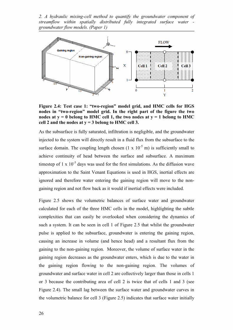
2. A hydraulic mixing-cell method to quantify the groundwater component of streamflow within spatially distributed fully integrated surface water - groundwater flow models. (Paper 1)
26
Figure 2.4: Test case 1: “two-region” model grid, and HMC cells for HGS nodes in “two-region” model grid. In the right part of the figure the two nodes at y = 0 belong to HMC cell 1, the two nodes at y = 1 belong to HMC cell 2 and the nodes at y = 3 belong to HMC cell 3.
As the subsurface is fully saturated, infiltration is negligible, and the groundwater
injected to the system will directly result in a fluid flux from the subsurface to the
surface domain. The coupling length chosen (1 x 10⁻⁵ m) is sufficiently small to
achieve continuity of head between the surface and subsurface. A maximum
timestep of 1 x 10⁻³ days was used for the first simulations. As the diffusion wave
approximation to the Saint Venant Equations is used in HGS, inertial effects are
ignored and therefore water entering the gaining region will move to the non-
gaining region and not flow back as it would if inertial effects were included.
Figure 2.5 shows the volumetric balances of surface water and groundwater
calculated for each of the three HMC cells in the model, highlighting the subtle
complexities that can easily be overlooked when considering the dynamics of
such a system. It can be seen in cell 1 of Figure 2.5 that whilst the groundwater
pulse is applied to the subsurface, groundwater is entering the gaining region,
causing an increase in volume (and hence head) and a resultant flux from the
gaining to the non-gaining region. Moreover, the volume of surface water in the
gaining region decreases as the groundwater enters, which is due to the water in
the gaining region flowing to the non-gaining region. The volumes of
groundwater and surface water in cell 2 are collectively larger than those in cells 1
or 3 because the contributing area of cell 2 is twice that of cells 1 and 3 (see
Figure 2.4). The small lag between the surface water and groundwater curves in
the volumetric balance for cell 3 (Figure 2.5) indicates that surface water initially

2. A hydraulic mixing-cell method to quantify the groundwater component of streamflow within spatially distributed fully integrated surface water - groundwater flow models. (Paper 1)
27
contributes more to the flow from the gaining region to the non-gaining region, as
the surface water is displaced by the groundwater. The SW and GW balances for
each of the HMC cells in the top panel of Figure 2.5 are also shown with the total
cell volume. Clearly, the SW and GW balances sum to the total volume,
indicating that that the HMC method conserves mass. The SW and GW fractions
for each of the HMC cells in the bottom panel of Figure 2.5 are seen from the
average of the two fractions to be inversely proportional to each other, as
expected. As the balances are calculated independently, this further highlights the
accuracy within the HMC method.
The relative error (�) in the balances is based on Eq. 2.7 and is determined using
the following equation:
��
��k
j
Nkif
1)(1�
(2.13)
The relative error relates to the accuracy of the numerical methods for solving the
flow equations, which is determined by the convergence criteria used in the
numerical scheme. This error grows slightly due to round-off errors and imperfect
balances in the numerical scheme used to solve the flow equations (finite
difference in this case). Such imperfect balances will always exist due to error in
the numerical scheme adopted, however they can be minimised by use of a small
value for the convergence criterion. In this test case the maximum relative error in
the HMC method was 1.5 x 10⁻³% in cell 1.
To investigate the effect of discretisation, the grid spacing dy in the flow direction
(y axis) is reduced in HGS from 1 m to 10 cm. As a result, the number of
corresponding cells in the HMC method increases to 21 (see Figure 2.6). Three
different simulations are then run to test the impact of time discretisation, with
constant time steps equal to 10-2, 10-3 and 10-4 days, respectively.
2. A hydraulic mixing-cell method to quantify the groundwater component of streamflow within spatially distributed fully integrated surface water - groundwater flow models. (Paper 1)
28
Figure 2.5: HMC cell, SW and GW balances (top panel) and fractions (bottom panel) for test case 1. The volumetric balance in the top row shows the HMC calculated balances for SW and GW in the HMC cells as well as the total volume in the cell which is calculated directly from the model outputs. The HMC cell SW and GW fractions in the bottom panel are calculated independently of each other.
The effects of temporal discretisation on the SW and GW fractions for the case of
dy = 10 cm are shown in Figure 2.7. In Figure 2.7, only the two end cells (1 and
21) and the middle cell (11) are shown. It can be seen that the finer timesteps
make little difference to the SW and GW fractions in cells 1 and 11, but that a
distinctly different solution of the SW and GW fractions arises in cell 21 for the
three timesteps used, with convergence at t = 10-3 and 10-4 days. It follows that it
is important to note that the timestep used in the model will dictate the SW and
GW fraction profiles in the HMC method. As highlighted in the theory, as dt
approaches zero, a perfectly mixed cell solution is approached. Variation in grid
size changes the representative area of the HMC cells. For example, halving the
grid size would result in the HMC cell area for the larger grid size being
represented by two HMC cells for the halved grid size. As the HMC cells are
representative of an area and not a point, results based on different grid
discretisations are not directly comparable. However, finer grids will give greater
spatial resolution of the SW and GW fractions along the surface. It follows that
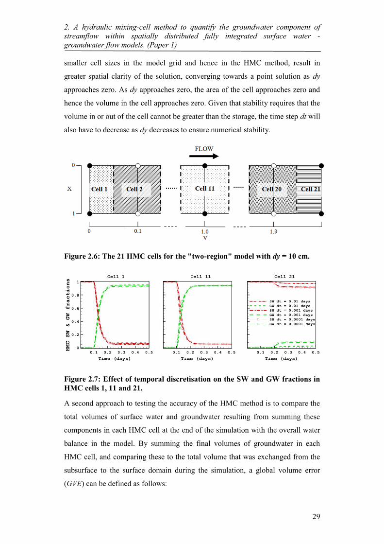
2. A hydraulic mixing-cell method to quantify the groundwater component of streamflow within spatially distributed fully integrated surface water - groundwater flow models. (Paper 1)
29
smaller cell sizes in the model grid and hence in the HMC method, result in
greater spatial clarity of the solution, converging towards a point solution as dy
approaches zero. As dy approaches zero, the area of the cell approaches zero and
hence the volume in the cell approaches zero. Given that stability requires that the
volume in or out of the cell cannot be greater than the storage, the time step dt will
also have to decrease as dy decreases to ensure numerical stability.
Figure 2.6: The 21 HMC cells for the "two-region" model with dy = 10 cm.
Figure 2.7: Effect of temporal discretisation on the SW and GW fractions in HMC cells 1, 11 and 21.
A second approach to testing the accuracy of the HMC method is to compare the
total volumes of surface water and groundwater resulting from summing these
components in each HMC cell at the end of the simulation with the overall water
balance in the model. By summing the final volumes of groundwater in each
HMC cell, and comparing these to the total volume that was exchanged from the
subsurface to the surface domain during the simulation, a global volume error
(GVE) can be defined as follows:

2. A hydraulic mixing-cell method to quantify the groundwater component of streamflow within spatially distributed fully integrated surface water - groundwater flow models. (Paper 1)
30
1001(%)
)(
��
����
�
�
N
NNSE
i
Ni
NGWi
tQ
VfGVE
(2.14)
Where QSEN [L3/T] is the summed exfiltration (SE) across the model domain at
time N from the overall water balance of HGS.
This measure gives the error of the HMC method relative to the summed
exfiltration from the overall water balance. The cumulative error of the HMC
method (as opposed to the instantaneous nodal fluid mass balance error in HGS)
will grow according to the convergence criteria, number of time steps and number
of stream cells. As the GVE is based on the summed exfiltration from the overall
water balance, it can only be used along completely gaining sections. It also
requires that all water is retained in the model domain (i.e. no losses). The
maximum relative error and GVE are given in Table 2.1 for the different spatial
and temporal discretisation tested, highlighting both the reduced maximum
relative error and GVE as the spatial and temporal resolution is increased.
Table 2.1: Maximum relative error in the HMC method, and the global volume error (GVE) for the HMC method.
HMC max. relative error GVE Timesteps
dy = 1m, t = 0.001 days 1.5 x 10⁻³% 1.97 x 10⁻⁴% 500 dy = 10cm, t = 0.01 days 1.8 x 10⁻⁴% 5.23 x 10⁻¹⁰% 50 dy = 10cm, t = 0.001 days 3.6 x 10⁻⁵% 1.17 x 10⁻¹⁰% 500 dy = 10cm, t = 0.0001 days 3.9 x 10⁻⁷% 2.81 x 10⁻¹¹% 5000
In the HMC cells of Test case 1, the relative and absolute errors are relatively
small and consequently the HMC method can be used in larger and more complex
model scenarios provided that fluid mass conservation is fulfilled.
2.3.3.2. Test case 2
The model setup for Test case 2 mirrors the physical processes of the catchment
shown in Figure 2.1. This test case is used to test not only the theoretical effects of
time lags (seen in the hydrographs of Figure 2.2) and accurate attribution and
tracking of streamflow generation mechanisms, but also to test the HMC method

2. A hydraulic mixing-cell method to quantify the groundwater component of streamflow within spatially distributed fully integrated surface water - groundwater flow models. (Paper 1)
31
in a highly transient model scenario whilst comparing the HMC method’s
groundwater component of streamflow with the summed exfiltration from the
overall water balance of the model.
Test case 2 is loosely based on the tilted V-catchment by Panday and Huyakorn
(2004), which has been used in verification of surface/subsurface interaction in
fully integrated models such as MOD-HMS and HGS. A number of modifications
are carried out to the V-catchment to mirror the spatial and temporal distribution
of the catchment shown in Figure 2.1. In order to distribute the subsurface to
surface exchange to the stream over its entire length, the slopes are reduced,
resulting in a significantly flatter catchment. The model domain shown in Figure
2.8 is 1000 m along the y axis by 810 m along the x axis (catchment area of
810,000 m2), with a homogeneous soil layer thickness of 20 m at (x = 800 – 810
m, y = 0 m) increasing in thickness with a gentle surface slope of 5 x 10⁻⁴ m/m
along the y axis (from y = 0 m to y = 1000 m) and 0.02 m/m along the x axis
(from x = 800 m to x = 0 m). With the use of the gentle slopes, the head gradient
required in order to produce an exchange from the subsurface to the surface along
the entire stream is achieved by raising the adjacent plane 2 m over a 5 m length
above the streambed as shown in the cross section of Figure 2.9.
Figure 2.8: Test case 2 catchment model (modified version of the V-catchment in Panday and Huyakorn (2004)). The contours correspond to the elevation.

2. A hydraulic mixing-cell method to quantify the groundwater component of streamflow within spatially distributed fully integrated surface water - groundwater flow models. (Paper 1)
32
Figure 2.9: Part cross section of hypothetical catchment highlighting the raised plane which is used to create a greater hydraulic gradient next to the stream leading to constant subsurface to surface exchange along the entire length (from x = 790 – 810 m, at y = 0 m and z = -4 to 2 m). The plane (left), bank (middle) and streambed (right) are seen in the division of top cells.
Grid spacing along the x axis is 50 m from x = 0 – 750 m, 25 m from x = 750 –
775 m, 15 m from x = 775 – 790 m, 5 m from x = 790 - 800 and 10 m from x =
800 – 810 m. The grid spacing is 50 m along the y axis and 1 m along the z axis
for the first 10 m below the surface with a thickness of 10 m to 26.5 m, varying
with the slopes of the catchment for the bottom layer. Streamflow at the
downstream boundary is governed by a critical depth boundary condition at the
end of the stream, which acts at nodes (800,0,0) and (810,0,0). The critical depth
boundary in HGS specifies the surface head to be at critical depth at the nodes
which are set with this boundary condition.
Saturation-relative permeability and saturation-pressure relationships are
described by the van Genuchten (1980) equations. The soil is a homogeneous
sand with the soil parameters derived from Carsel and Parrish (1988). The
surface friction is described using Manning’s n, with a value representing a
straight uniform channel (Chow, 1959), and a rill storage height and obstruction
height (as defined in Panday and Huyakorn (2004)) of 1 mm and 0 mm,
respectively. The rill storage height provides a threshold to surface flow whilst the
obstruction height provides retardation to flow. The surface and subsurface
parameters are detailed in Table 2.2. The coupling length (Eq. 2.12) is chosen
such that continuity of pressure at the surface/subsurface interface is maintained,
without jeopardising the accuracy of the flow solution. The solution of continuous

2. A hydraulic mixing-cell method to quantify the groundwater component of streamflow within spatially distributed fully integrated surface water - groundwater flow models. (Paper 1)
33
pressure at the surface/subsurface interface leads to much larger run times for the
simulations in this study (see Ebel et al., 2009), however for small coupling
lengths, the solution approaches that of continuous pressure at the
surface/subsurface interface.
Table 2.2: Surface and subsurface parameters for test case 2.
Parameter Value Surface Manning’s roughness 0.015 s/m1/3 Rill storage height 0.001 m Obstruction storage height 0.0 m Subsurface Porosity 0.1 Saturated hydraulic conductivity 8.25 x 10⁻⁵ m/s Van Genuchten � 14.5 m-1 Van Genuchten � 2.68 Residual saturation �r 0.045 Surface/Subsurface coupling Coupling length 0.5 m
The simulations for the hypothetical catchment are carried out in two phases:
1. Firstly, initial conditions are generated by running the model with a fully
saturated subsurface with only the critical depth forcing function in the surface
domain for approximately 40 days. This first simulation provides quasi steady-
state initial conditions for phase 2.
2. Based on these initial conditions the model is run for another 40 days with 3
rainfall events and constant groundwater pumping throughout the entire
simulation. The drawdown around the pump results in a losing section along a
part of the stream. Rainfall is applied across the entire catchment, starting at time t
= 0 seconds at a rate of 5.88 x 10⁻⁷ m/s (2.12 mm/hr) for a day at a time with three
recovery periods after each rainfall period of 10, 5 and 22 days, respectively for
each rainfall event. Pumping is applied at node (750,500,0) at a rate of -0.02 m3/s
throughout the simulation time. This extraction rate is sufficient to produce losses
over part of the stream. Over the length of the simulation there is a rainfall input
of 1.75 x 10⁵ m3 and a loss through pumping of 6.84 x 10⁴ m3. The maximum time

2. A hydraulic mixing-cell method to quantify the groundwater component of streamflow within spatially distributed fully integrated surface water - groundwater flow models. (Paper 1)
34
step used in the second phase of the simulation is 100 seconds. The rainfall and
pumping in the second phase create highly transient conditions. The length of the
stream that is losing is changing throughout the simulation. The nature of this
transience in the streamflow conditions allows for rigorous stability testing of the
HMC method because the stream cells are switching between gaining and losing
and are subject to sharp changes in volume and rate of change of volume in the
cell.
The rainfall events in the simulations provide recharge to the groundwater system,
sustaining flow to the stream. However, the gentle rainfall events and gentle
slopes in the catchment result in pure recharge with no overland flow on the
planes and hence no direct overland flow to the stream itself. Figure 2.10
highlights the changes in the subsurface to surface exchange, as well as the depth
and velocity along the stream at time = 1 second, 12 days and 40 days. At t =1
second in Figure 2.10, the initial stream is gaining along its entire length, before
groundwater abstraction has taken effect. At t = 12 days, there is an increased
discharge of groundwater at the top and bottom areas of the stream, which can be
attributed to the recharge resulting from rainfall as well as stream losses in the
middle section due to near stream groundwater extraction. The proportion of the
stream that is gaining and losing is varying throughout the entire simulation.
At t = 40 days, the subsurface to surface exchange to the stream has decreased
along the length of the stream due to the last rainfall event finishing 20 days
earlier. It also shows an increased loss from the stream over the middle losing
section due to reduced recharge in response to the groundwater extraction. This
loss rate from the stream in the middle causes the stream depth to drop over the
losing region, however streamflow is maintained through the entire simulation.
This qualitative analysis provides a reasonable understanding of the governing
processes in the system. For quantifying the groundwater component of
streamflow, the HMC method is required.
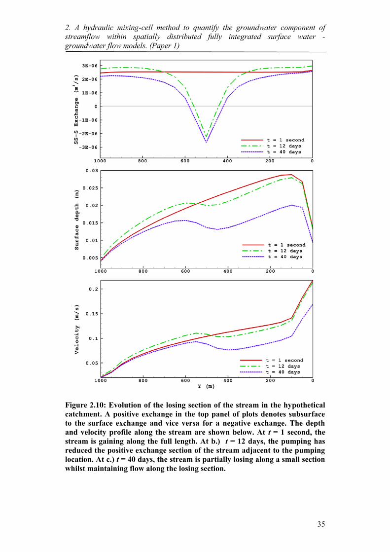
2. A hydraulic mixing-cell method to quantify the groundwater component of streamflow within spatially distributed fully integrated surface water - groundwater flow models. (Paper 1)
35
Figure 2.10: Evolution of the losing section of the stream in the hypothetical catchment. A positive exchange in the top panel of plots denotes subsurface to the surface exchange and vice versa for a negative exchange. The depth and velocity profile along the stream are shown below. At t = 1 second, the stream is gaining along the full length. At b.) t = 12 days, the pumping has reduced the positive exchange section of the stream adjacent to the pumping location. At c.) t = 40 days, the stream is partially losing along a small section whilst maintaining flow along the losing section.

2. A hydraulic mixing-cell method to quantify the groundwater component of streamflow within spatially distributed fully integrated surface water - groundwater flow models. (Paper 1)
36
The HMC method is applied to each pair of adjacent nodes that are located at x =
800 m and x = 810 m and that lie in the stream perpendicular to the direction of
flow. HMC cells are numbered from upstream (y = 1000m) to downstream (y =
0m) and correspond perfectly to the HGS cells. This gives rise to 21 HMC cells,
with 20 surface cells (x = 800 – 810 m and y = 0 – 1000 m) defined as the stream.
As a node based approach is used, the contributing area of nodes lying along x =
800 m takes into account the surface cells lying between x = 795 – 800 m. The
HMC maximum relative error in the simulation was 8.7 x 10⁻³% in HMC cell 13
at around t = 12 days.
The use of the HMC method allows the quantification of the groundwater
component of streamflow at any cell along the stream. Since the simulation set up
does not produce overland flow, the streamflow in each HMC cell consists of the
groundwater component and the direct rainfall component of streamflow. The
resultant groundwater component and direct rainfall fractions before and after the
first rainfall event for the HMC cells located at y = 0, 600 and 1000 m are shown
in Figure 2.11. In Figure 2.11, the rise and fall of the direct rainfall fraction is
sharp and fast in cell 1 and slower and longer in cells 13 and 21. This can be
attributed to the time lags of upstream flow that are evident at the downstream
cells and to the streamflow velocity in each cell. In Figure 2.10, the stream flow
velocity is seen to increase from the top of the stream (y = 1000 m) to the bottom
of the stream (y = 0 m) as water keeps entering the stream, although this is only
seen in the gaining regions. At t = 12 and 40 days, the stream is losing over the
middle section which is clearly evident in Figure 2.10 at around y = 400 m where
the velocity drops off only to start increasing again at y = 500 m. As surface flow
velocity is faster at the bottom sections of the catchment, storage effects alone can
be ruled out as causing the slower recession of the rainfall fraction in cells 13 and
21. The rainfall fraction after the first rainfall event (t = 1 day) in cells 13 and 21
must be due to rainfall from upstream cells in which there is a significant time lag
of approximately 0.2 days. It is also apparent that the rainfall fraction in cell 13 is
greater than the fraction in cell 21, which can be attributed to the increase in the
groundwater entering when moving downstream of cell 13. As there are only two
streamflow generation mechanisms in this simulation, the same explanation leads
to the groundwater component of streamflow results shown in Figure 2.11.
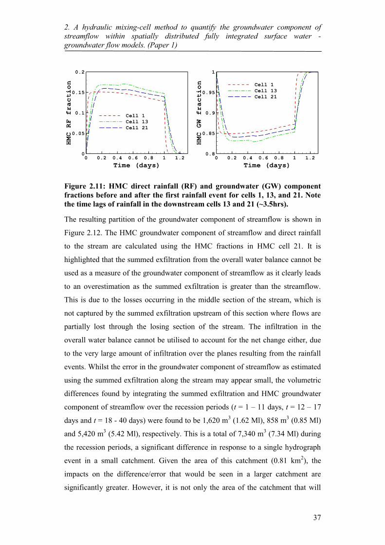
2. A hydraulic mixing-cell method to quantify the groundwater component of streamflow within spatially distributed fully integrated surface water - groundwater flow models. (Paper 1)
37
Figure 2.11: HMC direct rainfall (RF) and groundwater (GW) component fractions before and after the first rainfall event for cells 1, 13, and 21. Note the time lags of rainfall in the downstream cells 13 and 21 (~3.5hrs).
The resulting partition of the groundwater component of streamflow is shown in
Figure 2.12. The HMC groundwater component of streamflow and direct rainfall
to the stream are calculated using the HMC fractions in HMC cell 21. It is
highlighted that the summed exfiltration from the overall water balance cannot be
used as a measure of the groundwater component of streamflow as it clearly leads
to an overestimation as the summed exfiltration is greater than the streamflow.
This is due to the losses occurring in the middle section of the stream, which is
not captured by the summed exfiltration upstream of this section where flows are
partially lost through the losing section of the stream. The infiltration in the
overall water balance cannot be utilised to account for the net change either, due
to the very large amount of infiltration over the planes resulting from the rainfall
events. Whilst the error in the groundwater component of streamflow as estimated
using the summed exfiltration along the stream may appear small, the volumetric
differences found by integrating the summed exfiltration and HMC groundwater
component of streamflow over the recession periods (t = 1 – 11 days, t = 12 – 17
days and t = 18 - 40 days) were found to be 1,620 m3 (1.62 Ml), 858 m3 (0.85 Ml)
and 5,420 m3 (5.42 Ml), respectively. This is a total of 7,340 m3 (7.34 Ml) during
the recession periods, a significant difference in response to a single hydrograph
event in a small catchment. Given the area of this catchment (0.81 km2), the
impacts on the difference/error that would be seen in a larger catchment are
significantly greater. However, it is not only the area of the catchment that will

2. A hydraulic mixing-cell method to quantify the groundwater component of streamflow within spatially distributed fully integrated surface water - groundwater flow models. (Paper 1)
38
make use of the HMC method critical in determining the groundwater component
of streamflow generation. The travel time within the streams also undermines the
application of the summed exfiltration as seen in Figure 2.11. As the streams
become longer, the streamflow travel time from upstream to downstream
increases, and as such the summed exfiltration can be much sharper and
completely out of phase with the total streamflow as hypothesised in Figure 2.2.
The proportion and distribution of both gaining and losing sections also have a
clear effect of leading to overestimation of the groundwater component of
streamflow at the outlet.
Figure 2.12: Hyetograph for catchment and Hydrograph at the catchment outlet, showing separation of direct rainfall and groundwater components of streamflow, as well as the summed exfiltration from the overall water balance. The summed exfiltration (SE) from the water balance is clearly seen to exceed the outflow in this hypothetical catchment. The HMC direct rainfall and groundwater components of streamflow are calculated using the HMC fractions in HMC cell 21.
2.4. Discussion and Conclusions
The hydraulic mixing-cell (HMC) method developed in this paper overcomes
many of the limitations that exist in current methods of quantifying streamflow
generation mechanisms based on fully integrated spatially distributed SW-GW

2. A hydraulic mixing-cell method to quantify the groundwater component of streamflow within spatially distributed fully integrated surface water - groundwater flow models. (Paper 1)
39
interaction models. The HMC method accurately extracts streamflow generation
mechanisms using only hydraulic information. Streamflow generation
mechanisms at every HMC defined cell along the stream are extracted by post-
processing of the flow solution obtained from the numerical flow model. Because
the HMC method tracks the streamflow generation mechanisms along the stream,
temporal and spatial components that affect these mechanisms can be accounted
for. The HMC method correctly handles changing flow regimes (e.g. if a stream
changes from gaining to losing within the catchment), accounts for storage effects
within the channel and the time lags that occur within a catchment. These
attributes give the HMC method the ability to deal with the dynamic nature of
varying flow regimes in large and complex systems, such as the catchment
described in Figure 2.1. The only data requirements for the HMC method are the
fluxes at each cell and surface water depths, which are part of the flow solution.
By using this method, one does not have to make the commonly made
assumptions of negligible time lags in streamflow and exchanges being always
positive to the stream, in order to determine the streamflow generation
mechanisms.
In the current formulation, the HMC method is based on the modified mixing cell
(Campana and Simpson, 1984). Unless the mixing processes in the river are
explicitly simulated, the modified mixing rule has to be used. As highlighted in
the theory section, the HMC method is stable as long as the ratio of the volume of
water entering or leaving a HMC cell to the storage volume of the HMC cell is
less than unity. The assumption of constant river width and flow direction are
used in the coding of the HMC algorithm in this study. The initial formulation of
the HMC method presented here is based on the assumption of a constant river
width. In models such as HGS, the width of the stream can change in response to
a changing flowrate. In order to capture a changing river, the definition of the
river in the HMC algorithm must match the changes in the river. Further
development of the method is required to quantify streamflow generation
mechanisms in such systems. The HMC method presented is applicable (in
principle) to any spatially distributed flow modelling code, however the coding
requires generalisation to time varying river widths and lengths. The HMC

2. A hydraulic mixing-cell method to quantify the groundwater component of streamflow within spatially distributed fully integrated surface water - groundwater flow models. (Paper 1)
40
method should be routinely employed as either a subroutine within the model
code or a standard post processing tool in the new versions of the available codes.
Acknowledgements
This work is supported by the Australian Research Council through its Linkage
scheme and the South Australian Department of Water, Land and Biodiversity
Conservation as industry partners under grant number LP0668808. Parts of this
research were funded by the Swiss National Foundation, Ambizione grant
PZ00P2_126415. The views expressed in this paper are solely those of the
authors.

41
Chapter 3
3 Evaluation of outputs from automated baseflow separation methods against simulated baseflow from a physically based, surface water-groundwater flow model. (Paper 2)

42

43
Publication Details
This work has been published within the Journal of Hydrology as the following
article:
Partington, D., P. Brunner, C. T. Simmons, A. D. Werner, R. Therrien, G.
C. Dandy, and H. R. Maier. 2012. Evaluation of outputs from automated
baseflow separation methods against simulated baseflow from a physically
based, surface water-groundwater flow model. Journal of Hydrology, 458-
459: 28-39.
Although the manuscript has been reformatted in accordance with University
guidelines, and sections renumbered for inclusion within this thesis, the material
within this paper is otherwise presented herein as published.
Statement of Authorship
Partington, D. (Candidate)
Designed and conducted numerical experiments, coded baseflow analysis tool and
wrote manuscript.
Signed: . . . . . . . . . . . . . . . . . . . . . . . . . . . . . . . . . . . . . . . . . . . . . . . . Date: . . . . . . .
Brunner, P.
Supervised manuscript preparation and reviewed draft
Signed: . . . . . . . . . . . . . . . . . . . . . . . . . . . . . . . Date: . . . . . . .
Simmons, C.T.
Supervised manuscript preparation and reviewed draft
Signed: . . . . . . . . . . . . . . . . . . . . . . . . . . . . . . . . . . . . . . . . . . . . . . . . Date: . . . . . . .
Werner, A.D.
Supervised manuscrip d draft
Signed: . . . . . . . . . . . . . . . . . . . . . . . . . . . . . . . . . . . . . . . . . . . . . . . . Date: . . . . . . .
Therrien, R.
Supervised manuscrip
Signed: . . . . . . . . . . . . . . . . . . . . . Date: . . . . . . .

44
Maier, H. R.
Supervised manuscript preparation and reviewed draft
Signed: . . . . . . . . . . . . . . . . . . . . . . . . . . . . . . . . . . . . . . . . . . . . . . . . Date: . . . . . . .
Dandy, G. C.
Supervised manuscript preparation and reviewed draft
Signed: . . . . . . . . . . . . . . . . . . . . . . . . . . . . . . . . . . . . . . . . . . . . . . . . Date: . . . . . . .

3. Evaluation of outputs from automated baseflow separation methods against simulated baseflow from a physically based, surface water-groundwater flow model. (Paper 2)
45
Abstract
Baseflow is often considered to be the groundwater discharge component of
streamflow. It is commonly estimated using conceptual models, recursive filters
or a combination of the two. However, it is difficult to validate these methods due
to the current challenges of measuring baseflow in the field. In this study,
simulation of a synthetic catchment’s response to rainfall is carried out using a
fully integrated surface water-groundwater flow model. A series of rainfall events
with differing recovery periods and varied antecedent moisture conditions is
considered to span a range of different streamflow generation dynamics. Baseflow
is estimated for the outlet hydrograph of the synthetic catchment using a selection
of commonly used automated baseflow separation methods. These estimates are
compared to the baseflow signal obtained from the numerical model, which serves
as the control experiment. Results from these comparisons show that depending
on the method used, automated baseflow separation underestimates the simulated
baseflow by as much as 28%, or overestimates it by up to 74%, during rainfall
events. No separation method is found to be clearly superior to the others, as the
performance of the various methods varies with different soil types, antecedent
moisture conditions and rainfall events. The differences between the various
approaches clearly demonstrate that the baseflow separation methods investigated
are not universally applicable.
3.1. Introduction
Quantifying baseflow contributions to streamflow is of great interest in the
understanding, identification and quantification of streamflow generation
processes, in particular where baseflow supports important ecosystems and/or
provides critical dry season water supply (e.g. Smakhtin, 2001; Werner et al.,
2006). The term baseflow is often referred to as the groundwater contribution to
streamflow (e.g. Freeze, 1972; Brutsaert and Nieber, 1977; Eckhardt, 2005),
although it is also referred to as the release from both groundwater and other
natural storages of water that sustain streamflow between rainfall events (e.g.
Hall, 1968; Smakhtin, 2001; Piggott et al., 2005). In this paper, the term baseflow
is used to describe groundwater discharge that reaches the stream, not including
interflow through the vadose zone.

3. Evaluation of outputs from automated baseflow separation methods against simulated baseflow from a physically based, surface water-groundwater flow model. (Paper 2)
46
Baseflow can be inferred through field measurements of temperature, artificial
and natural tracer concentrations, and flow in seepage meters installed in stream
beds (Becker et al., 2004; Cook et al., 2003; Cook et al., 2008). However, for
practical reasons, it is very difficult to apply these techniques over an entire
catchment. Furthermore, the required end members in chemical mass balance
approaches are difficult to characterise (McCallum et al., 2010), which
complicates baseflow estimates using measurement of tracers. Consequently, the
available field methods do not currently allow accurate determination of spatially
and temporally distributed baseflow. In the absence of detailed field data, but
where a streamflow hydrograph is available, baseflow is therefore often estimated
using simple baseflow separation methods.
Since the early twentieth century, a variety of methods has been developed to
estimate baseflow. The earliest methods and some of the more recent ones are
based on a linear storage-discharge relationship between aquifer and stream (e.g.
Maillet, 1905; Barnes, 1939; Hall, 1968; Boughton, 1993). More recently, non-
linear storage-discharge relationships have also been applied to baseflow
separation (e.g. Wittenberg, 1994; Wittenberg and Sivapalan, 1999; Wittenberg,
2003) following theoretical studies suggesting that non-linear recessions are
appropriate for some catchments. Also, other methods that use some form of
hydrological reasoning have been developed without a physically based
mathematical framework. Currently, the separation of baseflow from the
streamflow hydrograph can be carried out utilising methods that can be grouped
into the following four categories: 1) graphical separation (Sloto and Crouse,
1996), 2) recession analysis (Tallaksen, 1995), 3) conceptual models (Barnes,
1939; Singh and Stall, 1971; Furey and Gupta, 2001; Eckhardt, 2005; Huyck et
al., 2005) and 4) recursive digital filters (Nathan and McMahon, 1990; Arnold
and Allen, 1999).
The different categories of separation approaches as noted above have been
compared and reviewed in several previous studies (Hall, 1968; Nathan and
McMahon, 1990; Arnold et al., 1995; Chapman, 1999; Smakhtin, 2001; Schwartz,
2007; Eckhardt, 2008). The reviews of Hall (1968), Smakhtin (2001) and
Schwartz (2007) provide a history of methods for baseflow separation, and discuss

3. Evaluation of outputs from automated baseflow separation methods against simulated baseflow from a physically based, surface water-groundwater flow model. (Paper 2)
47
the problems related to the definition of baseflow, as well as the underlying
assumptions of the different separation methods. In the context of identifying
groundwater recharge from streamflow records, the underlying assumptions that
underpin many methods were examined by Halford and Mayer (2000). They
concluded that identifying the groundwater contribution from streamflow records
can be ambiguous due to drainage exponentially decreasing from other sources,
such as bank storage, wetlands and the unsaturated zone. Furthermore, they noted
that simple automated methods are highly subjective with respect to their
algorithmic structure, and affected by the same underlying assumptions as other
more complex methods.
The analyses used in comparative studies to evaluate baseflow separation methods
(e.g. Nathan and McMahon, 1990; Arnold et al., 1995; Mau and Winter, 1997;
Chapman, 1999; Halford and Mayer, 2000; Schwartz, 2007; Eckhardt, 2008) are
often based on subjective measures, such as the plausibility of hydrological
behaviour, rather than a quantitative comparison to a known and well-quantified
baseflow hydrograph. This point was emphasised by Mau and Winter (1997) who
highlighted the need to validate baseflow estimates to avoid issues related to
subjective measures and other shortcomings of simplified methods. Unfortunately,
to date, no measured baseflow hydrograph at the catchment scale is available.
Until comprehensive data and better observation techniques come into existence,
numerical models, although theoretical, provide the best independent
conceptualisation of baseflow dynamics in catchments under different forcing
functions and hydrological conditions.
Some studies (e.g. Szilagyi, 2004; Fenicia et al., 2006; Ferket et al., 2010) have
compared baseflow estimated by separation methods with simulated baseflow
from lumped and semi-distributed catchment models. However, a critical analysis
of separation methods is inhibited by the lack of a reliable estimate of baseflow,
as well as some simplifications in the lumped and semi-distributed models, such
as the aquifer storage-discharge relationship (linear reservoir in Fenicia et al.
(2006), the sum of multiple linear reservoirs in Szilagyi (2004), and the
Boussinesq-equation in Ferket et al. (2010)).

3. Evaluation of outputs from automated baseflow separation methods against simulated baseflow from a physically based, surface water-groundwater flow model. (Paper 2)
48
More recently, physically based separation methods have been developed based
on process-based formulations of fluid mass balance equations of an aquifer (e.g.
Furey and Gupta, 2001; Furey and Gupta, 2003; Huyck et al., 2005). They
constitute an important step in overcoming the subjective elements of earlier
simpler methods, and attempt to alleviate some of their simplifying assumptions.
As well as the development of two physically based baseflow separation methods,
Furey and Gupta (2003) evaluated their methods against a complex physically
based numerical model of a hill-slope. Their study appears to be the first to
critically compare baseflow separation methods with a physically based numerical
model. However, by considering only the discharge from a single 2D synthetic
hill-slope (rather than a catchment), Furey and Gupta (2003) neglected important
catchment-scale processes, such as channel routing (e.g. streamflow attenuation
and translation) and channel losses (through losing sections, abstraction and
evaporation).
Fully integrated surface and subsurface flow models, some examples of which are
HydroGeoSphere (HGS) (Therrien et al., 2009), MODHMS (Hydrogeologic Inc.,
2006) and Parflow (Kollet and Maxwell, 2006), are useful for evaluating simpler
models because they do not need to assume a functional relationship between
baseflow and streamflow, or simple empirical relations. These models typically
represent 3D variably saturated subsurface flow with Richard’s equation, and 1D
and 2D surface flow with the diffusion wave approximation to the St. Venant
equations. A unique feature of fully integrated models is that water that is derived
from rainfall is allowed to partition into overland flow, streamflow, evaporation,
infiltration and recharge, whilst subsurface discharge to surface water features,
such as lakes and streams, occurs in a physically based fashion (Therrien et al.,
2009). Therefore, physically based numerical models provide an excellent means
for comparison of baseflow separation methods if the modelled baseflow
component of streamflow can be extracted.
Using physically based numerical models of 3D systems to evaluate baseflow
separation methods is difficult because the baseflow component of streamflow is
not a standard output. For a 2D hill-slope model, the baseflow component of
outflow is simply groundwater discharge. However, in the extension beyond 2D
3. Evaluation of outputs from automated baseflow separation methods against simulated baseflow from a physically based, surface water-groundwater flow model. (Paper 2)
49
hill-slopes, the baseflow component of simulated streamflow must be calculated
in some other way. As highlighted by Partington et al. (2011), the available
integrated models do not explicitly report the groundwater contribution to
streamflow. This problem is of particular importance for catchments where the
flow regime between surface water and groundwater is changing (e.g. gaining to
losing sections of a stream and vice versa). To overcome these difficulties,
Partington et al. (2011) developed a hydraulic mixing-cell (HMC) approach that
allows extraction of the groundwater contribution to streamflow within integrated
surface and subsurface flow models. Combining the HMC approach with the
HydroGeoSphere model, they demonstrated that spatiotemporal fluxes into and
out of a stream can be translated to a point along the stream allowing for
meaningful hydrograph separation. The HMC method allows for theoretical
examination of baseflow dynamics within a 3D catchment model, thus providing a
platform for comparison to automated baseflow separation methods.
In the current study, the HMC method is used in conjunction with HGS in order to
compare the outputs from a series of commonly used automated baseflow
separation methods. A numerical control experiment is developed using the
integrated model to simulate hydrological processes within a synthetic catchment.
Multiple simulations are carried out using differing initial, hydrologic and forcing
conditions in order to generate a series of outflow and baseflow hydrographs.
Baseflow separation methods are then applied to the outflow hydrographs from
the simulations. This allows comparison of the baseflow obtained from the
separation methods to the simulated baseflow. The commonly used separation
methods are based on graphical, conceptual and digital filter methods. The
analysis is limited to automated methods that are readily available and that only
rely on streamflow discharge data and catchment area. This analysis does not
include an assessment of more complex physically based methods. However, it is
noteworthy that this approach could also be used to test physically based methods,
e.g. those developed by Furey and Gupta (2001).
3.2. Methodology
The HydroGeoSphere (HGS) model used here is a fully integrated, physically
based model that simultaneously simulates 3D variably saturated subsurface flow

3. Evaluation of outputs from automated baseflow separation methods against simulated baseflow from a physically based, surface water-groundwater flow model. (Paper 2)
50
and 2D surface flow (Therrien et al., 2009). Water is exchanged between the
surface and subsurface domains through a first-order leakage relation based on the
head difference between the domains. The model also accounts for
evapotranspiration as a function of the leaf area index, soil moisture and root
depth. For further details on the numerical formulation and a review of the code,
the reader is referred to Park et al. (2009), Therrien et al. (2009) and Brunner and
Simmons (2011).
3.2.1. The synthetic catchment
The geometry of the catchment is loosely based on the tilted V-catchment
employed by Panday and Huyakorn (2004). As in Panday and Huyakorn (2004),
the catchment is symmetrical and therefore only half of the catchment is modelled
(shown in Figure 3.1). This particular geometry is an ideal synthetic framework
for generating hydrographs, because a range of hydrological processes control the
catchment’s behaviour. These processes include 3D saturated/unsaturated
groundwater flow, infiltration/exfiltration, overland flow and streamflow. An
analysis of the Panday and Huyakorn (2004) synthetic catchment highlighting
some of the issues associated with their model setup was undertaken by
Gaukroger and Werner (2011), and in response to these, several modifications to
the original setup are adopted here. The steep slopes and initially horizontal water
table in the Panday and Huyakorn (2004) case cause all groundwater discharge to
be concentrated around the outlet. Reducing the slope of the catchment
(particularly along the stream) creates a greater spatial distribution of the surface-
subsurface exchanges throughout the catchment. Therefore, the slopes
perpendicular and parallel to the stream are decreased from 0.05 m/m and 0.02
m/m to 0.002 m/m and 0.0005 m/m, respectively. Furthermore, the horizontal
water table represents an unrealistic (overly dry) initial condition. To start the
model from more realistic initial conditions, the catchment is saturated and
allowed to drain for between 7 and 9 months without any precipitation events. The
original roughness coefficients used for the hill-slope and stream domains cause
overland flow to be dominant parallel and adjacent to the stream, rather than in
the stream (Gaukroger and Werner, 2011). In order to allow overland flow to
discharge into the stream as it reaches the banks (rather than flowing alongside the

3. Evaluation of outputs from automated baseflow separation methods against simulated baseflow from a physically based, surface water-groundwater flow model. (Paper 2)
51
stream), the same roughness (0.015 s/m1/3) is used in both the overland flow and
stream domains. Also, the plane adjacent to the stream is raised by 0.6 m over a 5
m length to promote direct discharge of groundwater to the stream as opposed to
upslope exfiltration or return flow. Finally, the areal extent of the catchment is
increased from 810,000 m2 to 3,220,000 m2 by doubling the original length and
width of the catchment (keeping the stream width at 10 m). This reduces boundary
effects and increases aquifer storage capacity, which promotes sustained baseflow
contributions to the stream. Given the modifications outlined above, a wide range
of hydrographs can be generated by changing the forcing functions (e.g. rainfall,
groundwater pumping and evapotranspiration).
Figure 3.1: Modified tilted V-catchment used for simulation of the synthetic catchment’s rainfall response. Points 1 and 2 denote locations of groundwater pumps. Note that due to the symmetry of the catchment, only half of it is shown.
The bottom elevation of the model domain is set at -20 m relative to the 0 m
elevation of the streambed at the outlet. The aquifer properties are homogeneous
and isotropic. In separate model scenarios, two different sets of properties of the
aquifer material are considered (Table 3.1). Properties for evaporation and
transpiration are also included in Table 3.1.
The spatial discretisation in the catchment model is as follows: grid spacing along
the x axis is 50 m from x = 0 - 1550 m, 25 m from x = 1550 - 1575 m, 15 m from
x = 1575 - 1590 m, 5 m from x = 1590 - 1600 m and 10 m from x = 1600 - 1610
m. The grid spacing along the y axis is 50 m. The vertical grid discretisation

3. Evaluation of outputs from automated baseflow separation methods against simulated baseflow from a physically based, surface water-groundwater flow model. (Paper 2)
52
Table 3.1: Surface and subsurface parameters for the synthetic catchment model. For a detailed description of these model parameters see Therrien et al. (2009).
A NOTE:
This figure/table/image has been removed to comply with copyright regulations. It is included in the print copy of the thesis held by the University of Adelaide Library.

3. Evaluation of outputs from automated baseflow separation methods against simulated baseflow from a physically based, surface water-groundwater flow model. (Paper 2)
53
increases in thickness according to the slopes perpendicular and parallel to the
stream. Vertical discretisation along the z axis ranges from 0.25 m to 1 m for the
first 10 m below the surface. The time steps used in the model vary in accordance
with an adaptive time-stepping approach with a maximum step of 1000 seconds.
A no flow boundary is applied at the bottom and sides of the model domain. A
critical depth boundary is used at (x, y, z) = (1600 m, 0 m, 0 m) and (1610 m, 0 m,
0 m) to control the outflow at the stream outlet.
3.2.2. Baseflow calculation using the HMC method
The tracking of the streamflow generation mechanisms within a model simulation
requires the tracking of the spatiotemporal fluxes into, out of, and along the
stream. Parcels of groundwater discharging directly to the stream are “tracked”
using the HMC method (Partington et al., 2011) to allow determination of when
(and if) groundwater contributes to streamflow, as measured at the outlet (or at
any other location along the stream). The HMC method accounts for the travel
time along the stream and the spatiotemporal variation in the surface-subsurface
exchange fluxes, thereby separating the simulated streamflow hydrograph into
baseflow, overland flow and direct rainfall to the stream. A version of HGS that
has the HMC method incorporated into it is used to simulate the outlet hydrograph
of the synthetic catchment in response to a series of rainfall events, and
considering groundwater pumping and evapotranspiration. The calculated HMC
baseflow is used as the control experiment with which baseflow separations of the
simulated hydrograph are compared.
3.2.3. Baseflow separation using automated methods
The automated methods for baseflow separation used in this study are
implemented using the programs HYSEP (Sloto and Crouse, 1996), PART
(Rutledge, 1998) and BFLOW (Arnold and Allen, 1999). The Eckhardt filter
(Eckhardt, 2005) is also used. All of these approaches are well established
methods, are readily available, and were previously compared in the study of
Eckhardt (2008). However, they were judged subjectively based on hydrological
plausibility. Detailed descriptions of all approaches can be found in the above

3. Evaluation of outputs from automated baseflow separation methods against simulated baseflow from a physically based, surface water-groundwater flow model. (Paper 2)
54
cited literature, hence only a very brief overview of these methods is provided
below.
The HYSEP program allows the use of three curve fitting methods of hydrograph
separation; sliding interval (HYSEP1), fixed interval (HYSEP2) and local
minimum (HYSEP 3), as detailed in Pettyjohn and Henning (1979). For these
three methods, an empirical relationship is used, which relates the catchment area
to the number of days until baseflow makes up all streamflow, after a streamflow
peak.
PART uses a form of streamflow partitioning based on antecedent streamflow
recession (similar to the local minimum method of HYSEP), details of which are
given in Rutledge (1998). The determination of the antecedent recession
requirement in PART is done in three ways (see Rutledge, 1998) and thereby
provides three baseflow estimates: PART1, PART2 and PART3.
The BFLOW program uses the Lyne and Hollick (1979) filter, which is a low-pass
filter. This separation method uses signal processing theory, and is based on the
hydrological reasoning that baseflow is the low frequency component of
streamflow. The filter equation for baseflow is expressed as (Eckhardt, 2005):
tttttt QbQQbb ��
��� �� tosubject)(
21
11�� (3.1)
Where bt [L3/T] is the baseflow at time step t [T], � [dimensionless] is the filter
parameter and Qt [L3/T] is the streamflow at time step t. It is worth noting the
constraint tQtb � , which is required in applying (1) to avoid predictions of
baseflow greater than streamflow (Chapman, 1991; Eckhardt, 2005). This
constraint is discussed further in Section 3.4.3. The BFLOW program carries out
three passes of the filter: forwards (BFLOW1), backwards (BFLOW2) and
forwards again (BFLOW3) and uses a filter parameter � = 0.925 as suggested by
Nathan and McMahon (1990). Each pass of the filter acts to attenuate the
baseflow signal. Despite having no physical basis, the baseflow separation of
BFLOW has been found to agree well with manual separation techniques (Arnold
and Allen, 1999).
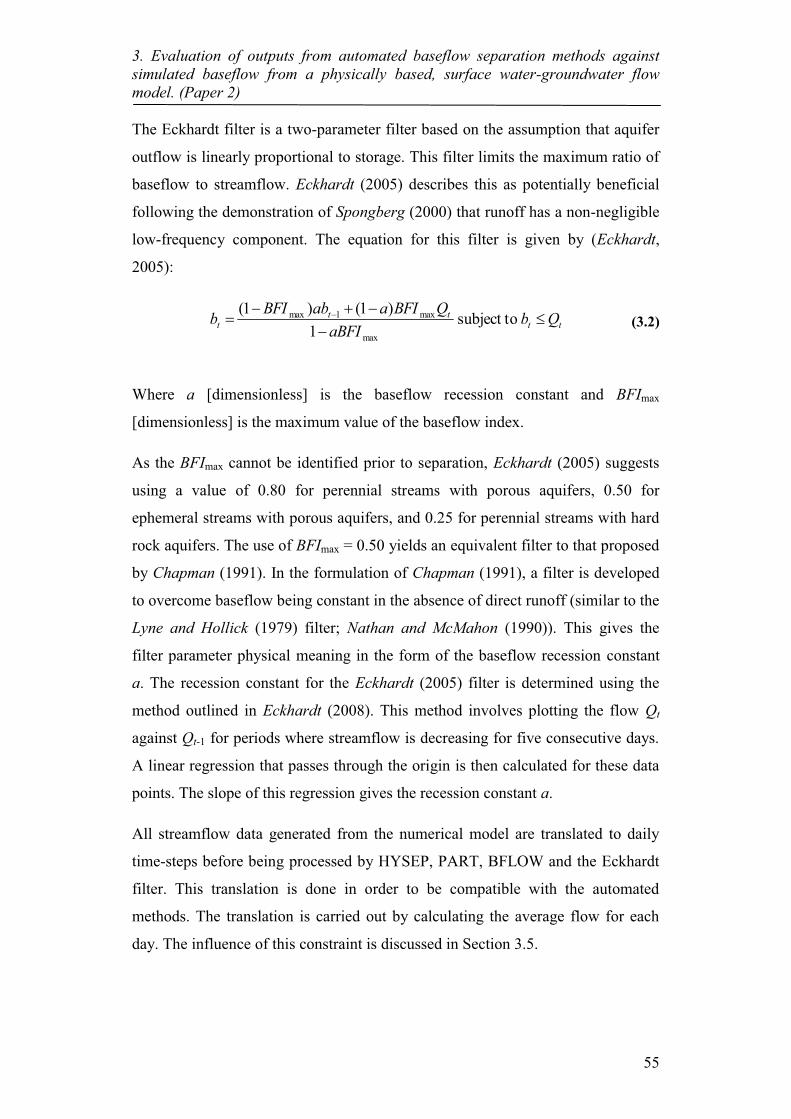
3. Evaluation of outputs from automated baseflow separation methods against simulated baseflow from a physically based, surface water-groundwater flow model. (Paper 2)
55
The Eckhardt filter is a two-parameter filter based on the assumption that aquifer
outflow is linearly proportional to storage. This filter limits the maximum ratio of
baseflow to streamflow. Eckhardt (2005) describes this as potentially beneficial
following the demonstration of Spongberg (2000) that runoff has a non-negligible
low-frequency component. The equation for this filter is given by (Eckhardt,
2005):
tt
ttt Qb
aBFIQBFIaabBFIb �
����
� � tosubject1
)1()1(
max
max1max
(3.2)
Where a [dimensionless] is the baseflow recession constant and BFImax
[dimensionless] is the maximum value of the baseflow index.
As the BFImax cannot be identified prior to separation, Eckhardt (2005) suggests
using a value of 0.80 for perennial streams with porous aquifers, 0.50 for
ephemeral streams with porous aquifers, and 0.25 for perennial streams with hard
rock aquifers. The use of BFImax = 0.50 yields an equivalent filter to that proposed
by Chapman (1991). In the formulation of Chapman (1991), a filter is developed
to overcome baseflow being constant in the absence of direct runoff (similar to the
Lyne and Hollick (1979) filter; Nathan and McMahon (1990)). This gives the
filter parameter physical meaning in the form of the baseflow recession constant
a. The recession constant for the Eckhardt (2005) filter is determined using the
method outlined in Eckhardt (2008). This method involves plotting the flow Qt
against Qt-1 for periods where streamflow is decreasing for five consecutive days.
A linear regression that passes through the origin is then calculated for these data
points. The slope of this regression gives the recession constant a.
All streamflow data generated from the numerical model are translated to daily
time-steps before being processed by HYSEP, PART, BFLOW and the Eckhardt
filter. This translation is done in order to be compatible with the automated
methods. The translation is carried out by calculating the average flow for each
day. The influence of this constraint is discussed in Section 3.5.

3. Evaluation of outputs from automated baseflow separation methods against simulated baseflow from a physically based, surface water-groundwater flow model. (Paper 2)
56
3.3. Model Simulations
To provide varied catchment responses and streamflow regimes, the synthetic
catchment is subjected to varied rainfall and antecedent moisture conditions.
These different conditions are used to examine the extent to which the HYSEP,
BFLOW, PART and the Eckhardt separation methods reproduce and capture the
HMC calculated baseflow signal. Two of the simulations are also subject to near-
stream groundwater pumping. The simulations with groundwater pumping allow
investigation into the common scenario of a modified catchment. Although some
separation methods are specified for use in undisturbed catchments, they are still
applied in this study to simulations with pumping. However, for this reason, the
simulations with pumping are considered separately from the simulations without
pumping. The baseflow separation methods are evaluated quantitatively and
qualitatively against the simulated baseflow using measures that account for total
baseflow volume, as well as baseflow dynamics.
Initially, eight model scenarios are simulated (Table 3.2). The first three scenarios
(1, 2 and 3) consider the influence of pumping for the sandy catchment. Scenarios
4 and 5 consider different initial conditions as the starting points for scenarios 4
and 5, respectively. Scenarios 6, 7 and 8 consider a change in soil properties of the
sand to loamy sand. As well as providing the controlled baseflow signal for
evaluation of baseflow separation methods, the variation of aquifer properties
provides insight into their influence on streamflow generation mechanisms.
Table 3.2: Scenarios for simulating catchment response. Scenarios with an asterisk denote scenarios where groundwater pumping is applied in the catchment.
Scenario Soil Initial Water table Pumping 1 Sand WT3 -
2* Sand WT3 pump 1 3* Sand WT3 pump 1and 2 4 Sand WT2 - 5 Sand WT1 - 6 Loamy sand WT3 - 7 Loamy sand WT2 - 8 Loamy sand WT1 -

3. Evaluation of outputs from automated baseflow separation methods against simulated baseflow from a physically based, surface water-groundwater flow model. (Paper 2)
57
The initial hydraulic heads and water table elevations are obtained by draining the
fully saturated catchment for a period of 7, 8 and 9 months without applying any
rainfall forcing or subsurface boundary recharge. The initial conditions used are:
water table 1 (WT1) = 7 months drainage, water table 2 (WT2) = 8 months
drainage and water table 3 (WT3) = 9 months drainage. For each of these initial
conditions the stream is still flowing at the end of the drainage period, whilst
providing significantly different initial conditions.
The catchment’s response is controlled by modifying the forcing functions (e.g.
rainfall, pumping and ET) to scenarios with a series of different initial conditions.
The rainfall varies in intensity and duration over three rain events throughout each
of the simulations. The same rainfall boundary is applied in each of the eight
scenarios as follows:
1) 10 days without rainfall, then rainfall at a rate of 2 mm/h for 24 h followed by
10 days without rainfall; and
2) rainfall at a rate of 4 mm/h for 48 h followed by 5 days without rainfall; and
3) rainfall at a rate of 40 mm/h for 3 h followed by 30 days without rainfall (58
days and 3 h total)
The idealised rainfall events are uniform and constant with sufficiently large
recovery periods such that the streamflow generation processes resulting from
individual events can be clearly identified. The rainfall rates and durations are
chosen to represent a range of streamflow generation mechanisms.
Pumping is applied in scenarios 2 and 3 at two locations (shown in Figure 3.1):
Pump 1 located at (x, y, z) = (1550 m, 500 m, 0 m), and pump 2 located at (x, y, z)
= (1550 m, 1500 m, 0 m). The pumping rate is increased linearly from 0.00 to
0.01 m3/s for pump 1 over the first day of simulation in scenario 2, with pump 2
inactive. In scenario 3, the pumping rate is increased linearly from 0.00 to 0.015
m3/s for both pumps 1 and 2 over the first day of simulation. For scenarios 2 and
3, pumping is applied over the entire simulation. This pumping rate induces losing
conditions locally along the stream near the pumping location. Pumping therefore

3. Evaluation of outputs from automated baseflow separation methods against simulated baseflow from a physically based, surface water-groundwater flow model. (Paper 2)
58
allows the effect of varied flow regimes (i.e. gaining and losing sections) on
streamflow generation to be explored with respect to baseflow.
Based on the initial simulations, evapotranspiration (ET) is applied to 5 additional
scenarios (denoted as 9, 10, 11, 12 and 13; not listed in Table 3.2). The setup and
forcing functions of scenarios 9, 10, 11, 12 are the same as for scenario 1, except
that constant specified evaporation rates of 2, 5, 10 and 26 mm/day are applied,
respectively. Some high evaporation rates (10 and 26 mm/day) are chosen to
explore the influence that high ET in the catchment has on the baseflow
separation methods. ET is also applied to scenario 13 with the same setup and
forcing functions as for scenario 6, but with a constant specified evaporation rate
of 5 mm/day. The simulations with ET are performed in order to examine the
influence of ET on baseflow dynamics, baseflow recession and performance of
separation methods against the simulated baseflow.
3.4. Results
3.4.1. Fully integrated model simulations
The simulated streamflow hydrograph at the outlet and the corresponding
streamflow generation components (calculated from the HMC method) are shown
for scenarios 1 (Figure 3.2) and 2 (Figure 3.3). The streamflow generation
mechanisms varied in response to different rainfall events. In all scenarios that
were based on sandy material properties, streamflow was dominated by baseflow
because the high infiltration capacity of the sand allowed for quick recharge.
Consequently, there was only a small overland flow component due to saturation
excess runoff. The almost horizontal slope of the catchment limited the vertical
extent of the unsaturated zone to less than 1 m, resulting in a short delay between
infiltration and recharge. As the timing between infiltration and recharge was
short, there was a rapid response in the baseflow component of streamflow. As
illustrated in Figure 3.2, after a short and rapid initial increase, baseflow did not
change significantly during the first two rainfall events and reached an apparent
steady-state. As opposed to baseflow, streamflow changed during this apparent
steady-state. Therefore, the ratio of streamflow to baseflow changes as a function
of time, but not consistently across events.

3. Evaluation of outputs from automated baseflow separation methods against simulated baseflow from a physically based, surface water-groundwater flow model. (Paper 2)
59
The apparent steady-state baseflow was only observed during the first two events.
However, in the third event no apparent steady-state was reached. In this event, an
initial rapid increase in head in the subsurface quickly increased the hydraulic
gradient from the aquifer to the stream. During this rainfall event, the time delay
from rainfall starting to the onset of overland flow is much slower than the time
delay to the increase in groundwater discharge caused by the rapid aquifer
response. After 1 hour, the overland flow and accumulating direct rainfall to the
stream increased the stream stage, thus reducing the hydraulic gradient between
the aquifer and stream. This is a clear demonstration of the forcing functions
controlling the baseflow dynamics.
The baseflow response from all three rainfall events did not follow the typical
pattern of baseflow response as presented in standard textbooks, e.g. McCuen
(2005) and Linsley et al. (1958). This is an important observation because these
patterns are the basis for graphical approaches of baseflow separation. The pattern
of baseflow during rainfall events obtained from the HGS model demonstrated a
fast and transient response in stream-aquifer interaction. This was apparent at the
beginning and cessation of the rainfall events, where an abrupt change in baseflow
occurs, rather than a smooth and delayed response. The high transience of the
stream aquifer interaction was also apparent in scenarios 2 and 3. The drawdown
around the pump induced a loss in the adjacent stream, creating a variable flow
regime with dynamic losing and gaining sections. The drawdown also increased
the time between infiltration and recharge, further affecting the system dynamics.
The effect of ET (at a rate of 5 mm/day) is shown in Figure 3.4 for the example of
scenario 10. In comparison to scenario 1, the inclusion of ET in scenarios 9, 10,
11 and 12 slightly reduced event peaks and the baseflow component. These
changes are due to the reduction in storage through losses from ET. However, it
can be seen by comparison of Figure 3.2 and Figure 3.4, that the baseflow
dynamics were very similar; the reduced overland flow component lead to a
slightly higher proportion of baseflow with respect to streamflow.

3. Evaluation of outputs from automated baseflow separation methods against simulated baseflow from a physically based, surface water-groundwater flow model. (Paper 2)
60
Figure 3.2: Streamflow hydrograph at the outlet and HMC flow components for scenario 1 (without pumping), with highlighted events. An apparent steady-state baseflow rate was observed in the first event (10.5-11 days) and second event (21.4-23 days).
Figure 3.3: Streamflow hydrograph at the outlet and HMC flow components for scenario 2 (with pumping), with highlighted events. An apparent steady-state baseflow rate was observed in the first two rainfall events.
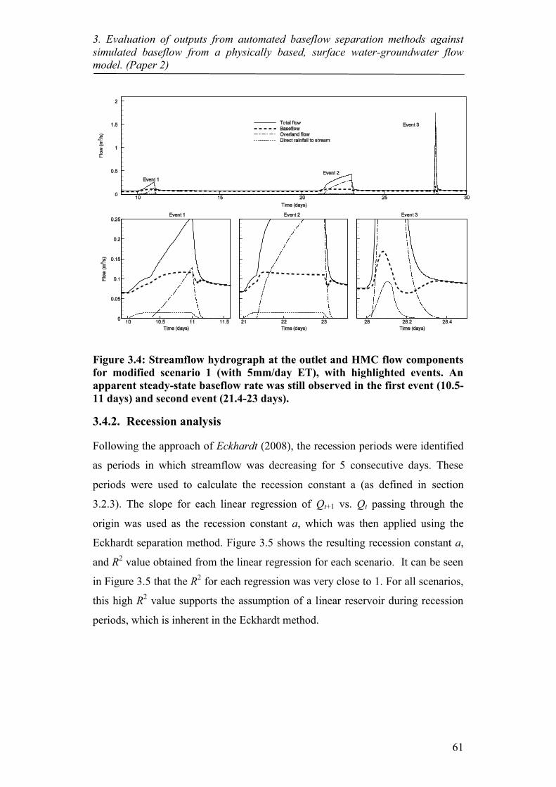
3. Evaluation of outputs from automated baseflow separation methods against simulated baseflow from a physically based, surface water-groundwater flow model. (Paper 2)
61
Figure 3.4: Streamflow hydrograph at the outlet and HMC flow components for modified scenario 1 (with 5mm/day ET), with highlighted events. An apparent steady-state baseflow rate was still observed in the first event (10.5-11 days) and second event (21.4-23 days).
3.4.2. Recession analysis
Following the approach of Eckhardt (2008), the recession periods were identified
as periods in which streamflow was decreasing for 5 consecutive days. These
periods were used to calculate the recession constant a (as defined in section
3.2.3). The slope for each linear regression of Qt+1 vs. Qt passing through the
origin was used as the recession constant a, which was then applied using the
Eckhardt separation method. Figure 3.5 shows the resulting recession constant a,
and R2 value obtained from the linear regression for each scenario. It can be seen
in Figure 3.5 that the R2 for each regression was very close to 1. For all scenarios,
this high R2 value supports the assumption of a linear reservoir during recession
periods, which is inherent in the Eckhardt method.
3. Evaluation of outputs from automated baseflow separation methods against simulated baseflow from a physically based, surface water-groundwater flow model. (Paper 2)
62
Figure 3.5: Values of recession constant a and R2 value for the linear regression of Qt vs Qt+1, for sand and initial conditions WT1, WT2, WT3 and without/with pumps 1 and 2 active. The high value of R2 suggests a linear storage-discharge relationship at the outlet during recession periods.
Adding ET in scenarios 9 to 13 reduced slightly the recession constant a, by less
than 2% and it also slightly reduced the linearity of the storage-discharge
relationship (R2 > 0.96) of the catchment during recession periods. The linearity
assumption for the storage-discharge relationship for this synthetic catchment was
therefore still deemed reasonable.
3.4.3. Comparison of baseflow separation methods
All of the automated separation methods used are subject to the condition that
baseflow cannot exceed streamflow. This is imposed because without this
constraint, all of these methods can yield baseflow estimates above streamflow.
By contrast, Furey and Gupta (2001) suggested that such a condition should not
be imposed on physically-based methods. This way it is possible to identify time
periods where estimated baseflow exceeds streamflow and diagnose these
estimation errors. Steps can then be taken to modify the method while honouring
physical processes so that these errors are reduced or fully removed. This
constraint has repercussions for our analysis. In recession periods, the baseflow
calculated from the automated separation methods is perfectly matched to the
HMC calculated baseflow, because streamflow is entirely composed of baseflow.
Therefore, an assessment of the differences between the simulated and
approximated baseflow hydrographs is only meaningful during rainfall events.
Consequently, this comparison is carried out during the rainfall events (i.e. 10-13

3. Evaluation of outputs from automated baseflow separation methods against simulated baseflow from a physically based, surface water-groundwater flow model. (Paper 2)
63
days, 21-25 days and 28-30 days) with the commonly used ratio of baseflow to
streamflow, and two statistical measures, as follows:
a) the baseflow index (BFI), which is the ratio of the total baseflow volume to the
total streamflow volume over a given period:
streamflow
baseflow
VV
BFI �
(3.3)
Where Vbaseflow [L3] and Vstreamflow [L3] are the total volume of baseflow and
streamflow, respectively, over the simulation period.
b) the Nash-Sutcliffe model efficiency (NSE) coefficient:
��
�
�
�
��� T
t oto
T
ttm
to
bb
bbNSE
12
12
)(
)(1
(3.4)
Where bot [L3/T] is the HMC calculated baseflow at time step t [T], bm
t [L3/T] is
the baseflow from automated separation at time step t [T], and ob [L3/T] is the
mean HMC calculated baseflow. The NSE provides a measure with values ranging
from -∞ to 1 (where 1 indicates a perfect match), of how well the separation
methods compare to the HMC calculated baseflow. Moriasi et al. (2007) suggest
that a NSE > 0.5 is satisfactory.
And c) the percent bias (PBIAS) (Gupta et al., 1999):
��
�
���
� T
tto
T
ttm
to
b
bbPBIAS
1
1
)(
100)(
(3.5)
The PBIAS provides a measure of over or underestimation for each event, with an
optimal value of 0%. Positive values of PBIAS indicate an underestimation,
whereas negative values indicate overestimation of baseflow. Moriasi et al.
(2007) suggest that a PBIAS of up to ±25% for streamflow is satisfactory, and this
is used to guide acceptable PBIAS results in this study.

3. Evaluation of outputs from automated baseflow separation methods against simulated baseflow from a physically based, surface water-groundwater flow model. (Paper 2)
64
The baseflow index (BFI), Nash-Sutcliffe efficiency (NSE) and percent bias
(PBIAS) are given for each of the three rainfall events in Table 3.3,Table 3.4, and
Table 3.5, respectively, for scenarios 1-8. The values for NSE < 0.5 and │PBIAS│
> 25% are highlighted. The BFIs calculated across the entire simulation for each
scenario are ranked for each separation method in Figure 3.6. Ranking is in order
of best to worst BFI relative to the BFI observed from the HGS model (based on
the HMC calculated baseflow). The results for the testing of the inclusion of ET
for scenario 1 are shown in Table 3.6.
For event 1, the NSEs were satisfactory over all scenarios for HYSEP2, PART1,
PART2, PART3, BFLOW1, BFLOW2 and the Eckhardt separation methods.
However, in scenario 3, HYSEP1, HYSEP3 and BFLOW3 had a NSE less than
0.5, with BFLOW3 showing a very unsatisfactory performance indicated by a
negative NSE. The BFLOW1 separation had a single instance of NSE less than 0.5
and the Eckhardt separation had two instances of NSE less than 0.5. However,
these were only slightly below this value, indicating that the performance of these
methods was almost satisfactory. The PBIAS was at a maximum of 33.8% for
event 1 of scenario 3 for the BFLOW3 separation method, showing a large
underestimation of the HMC calculated baseflow. All separation methods for
event 1 tended to underestimate baseflow. Only BFLOW1 overestimated
baseflow, which occurred for the sandy loam in scenarios 6-8.
For event 2, the NSEs were below 0.5 for each separation method in at least one of
the eight scenarios. The BFLOW3 separation showed very poor performance with
negative NSEs in scenarios 2-5. In each of these scenarios, BFLOW3 had a PBIAS
showing underestimation of baseflow by more than 25%. The HYSEP1, HYSEP2,
BFLOW1 and Eckhardt methods showed poor performance for sandy loam
(scenarios 6-8) with negative NSEs in each scenario. The PBIAS for HYSEP1 and
BFLOW1 separation showed overestimation of baseflow ranging from 40%-73%
in the sandy loam scenarios. It is interesting to note that the scenarios in which
HYSEP1, HYSEP2 and BFLOW1 performed well, HYSEP3, PART1, PART2,
PART3, BFLOW2 and BFLOW3 performed poorly and vice versa.

3. Evaluation of outputs from automated baseflow separation methods against simulated baseflow from a physically based, surface water-groundwater flow model. (Paper 2)
65
Tab
le 3
.3: B
FI,
NSE
and
PB
IAS
for
sim
ulat
ed b
asef
low
and
est
imat
ed b
asef
low
dur
ing
even
t 1 u
sing
HY
SEP,
PA
RT
, BFL
OW
an
d th
e E
ckha
rdt s
epar
atio
n m
etho
ds. L
ight
ly s
hade
d ce
lls h
ighl
ight
a N
SE <
0.5
and
dar
kly
shad
ed c
ells
hig
hlig
ht │
PBIA
S│ >
25
%. S
cena
rios
with
an
aste
risk
den
ote
whe
re g
roun
dwat
er p
umpi
ng is
app
lied
in th
e ca
tchm
ent.

3. Evaluation of outputs from automated baseflow separation methods against simulated baseflow from a physically based, surface water-groundwater flow model. (Paper 2)
66
Tab
le 3
.4: B
FI,
NSE
and
PB
IAS
for
sim
ulat
ed b
asef
low
and
est
imat
ed b
asef
low
dur
ing
even
t 2 u
sing
HY
SEP,
PA
RT
, BFL
OW
and
th
e E
ckha
rdt s
epar
atio
n m
etho
ds. L
ight
ly s
hade
d ce
lls h
ighl
ight
a N
SE <
0.5
and
dar
kly
shad
ed c
ells
hig
hlig
ht │
PBIA
S│ >
25%
. Sc
enar
ios w
ith a
n as
teri
sk d
enot
e w
here
gro
undw
ater
pum
ping
is a
pplie
d in
the
catc
hmen
t.

3. Evaluation of outputs from automated baseflow separation methods against simulated baseflow from a physically based, surface water-groundwater flow model. (Paper 2)
67
Tab
le 3
.5:
BFI,
NSE
and
PBI
AS
for
simul
ated
bas
eflo
w a
nd e
stim
ated
bas
eflo
w d
urin
g ev
ent
3 us
ing
HY
SEP,
PA
RT
, B
FLO
W a
nd t
he
Eck
hard
t sep
arat
ion
met
hods
. Lig
htly
shad
ed c
ells
high
light
a N
SE <
0.5
and
dar
kly
shad
ed c
ells
hig
hlig
ht │
PBIA
S│ >
25%
. Sce
nari
os w
ith a
n as
teri
sk d
enot
e w
here
gro
undw
ater
pum
ping
is a
pplie
d in
the
catc
hmen
t.

3. Evaluation of outputs from automated baseflow separation methods against simulated baseflow from a physically based, surface water-groundwater flow model. (Paper 2)
68
Tab
le 3
.6: C
ompa
riso
n of
BFI
, NSE
and
PBI
AS
for
(sce
nari
o 1
with
and
with
out E
T) si
mul
ated
bas
eflo
w a
nd e
stim
ated
bas
eflo
w d
urin
g ev
ent 2
us
ing
HY
SEP,
PA
RT
, BFL
OW
and
the
Eck
hard
t se
para
tion
met
hods
. Lig
htly
sha
ded
cells
hig
hlig
ht a
NSE
< 0
.5 a
nd d
arkl
y sh
aded
cel
ls hi
ghlig
ht │
PBIA
S│ >
25%
.

3. Evaluation of outputs from automated baseflow separation methods against simulated baseflow from a physically based, surface water-groundwater flow model. (Paper 2)
69
More interestingly, where the HYSEP1, HYSEP2 and BFLOW1 methods
performed poorly, these methods largely overestimated baseflow whereas where
the HYSEP3, PART1, PART2, PART3, BFLOW2 and BFLOW3 methods
performed poorly, these particular methods largely underestimated baseflow.
For event 3, the NSE was greater than 0.5 for every method in each scenario, with
values close to 1. The largest PBIAS was for BFLOW3 in scenario 3, showing
underestimation of baseflow by just over 25%.
The inclusion of ET in scenarios 9-13 showed that as the ET rate was increased,
the BFI increased. ET also lead to a reduction in performance (both NSE and
PBIAS) for every separation method, except HYSEP1.
The rankings of separation methods (shown in Figure 3.6) based on BFI over the
entire simulation provide a summary of the performance of each of the separation
methods. The best replication of BFI resulted from the HYSEP1 method in
scenarios 1-5, from PART1 in scenario 6, and from HYSEP2 in scenarios 7-8.
The BFLOW3 method was worst in scenarios 1-3 and 8. The Eckhardt method
performed worst in scenarios 4 and 5.
Figure 3.6: Performance based ranking using BFI over the whole simulation for HYSEP, PART, BFLOW and the Eckhardt separation methods. 1 indicates best performance, 10 indicates worst performance.
The baseflow separations from the streamflow hydrograph in scenario 1 obtained
using HYSEP, PART, BFLOW and the Eckhardt separation methods are shown in
Figure 3.7. Visual inspection of baseflow curves in Figure 3.7 shows that the
ability of these separation methods to match the simulated baseflow was poor in
1 2 3 4 5 6 7 8 9
10
1 2 3 4 5 6 7 8
Perf
orm
ance
Ran
king
Scenario
HYSEP1 HYSEP2 HYSEP3 PART1 PART2 PART3 BFLOW1 BFLOW2 BFLOW3 ECKHARDT

3. Evaluation of outputs from automated baseflow separation methods against simulated baseflow from a physically based, surface water-groundwater flow model. (Paper 2)
70
almost all cases, despite the fact that they had satisfactory NSE and PBIAS values.
It is clear that despite reasonable estimates of the BFI for each scenario, the
dynamics of baseflow during rainfall were missed.
Figure 3.7: Comparison of simulated daily baseflow and baseflow estimated using HYSEP, PART, BFLOW and the Eckhardt separation methods for scenario 1.
3.5. Discussion
The baseflow hydrographs obtained using HGS (with the HMC method) were
used as a control experiment to test the performance of a series of automated
baseflow separation methods. The initial conditions (antecedent moisture), forcing
functions (rainfall patterns, pumping and ET) as well as the physical properties
(soil properties) of the catchment were varied across simulation scenarios. The
varied conditions across the different model scenarios allowed the generation of
unique baseflow behaviour, controlled by a range of hydrological processes. The
application of the HMC method allowed quantification of the relative importance
of hydrological processes to the streamflow hydrograph. While the structure and
geology of the synthetic model used in this study were simple, the hydrological
processes considered were simulated in a physically based way. Despite the
simplified nature of the catchment, the baseflow separation methods consistently

3. Evaluation of outputs from automated baseflow separation methods against simulated baseflow from a physically based, surface water-groundwater flow model. (Paper 2)
71
failed to perform satisfactorily. This is easily attributed the variability of the
baseflow dynamics as observed across all simulation scenarios. Increasing the
complexity of the catchment (e.g. heterogeneous geology, more realistic
topography and rainfall patterns), is likely to lead to an even more complex
baseflow response. With increased complexity, it is expected that the variability
seen in baseflow dynamics will remain and hence that the simple automated
baseflow separation methods examined will not perform any better in estimating
baseflow.
An initial analysis of the hydrographs revealed that the behaviour of baseflow was
fundamentally different between rainfall events. For the first two events, baseflow
remained constant and reached an apparent steady-state despite the changing
forcing functions. In contrast, baseflow dynamics during the third event were
highly transient. This illustrates that the controlling processes of baseflow are not
always static, but instead change in response to different forcing functions. It also
challenges the common assumption (based on hydrological reasoning) of the
simple automated baseflow separation methods, that a simple fixed relation
between baseflow and streamflow exists, for all rainfall events and antecedent
moisture conditions. It is observed that this is not necessarily the case.
In the synthetic catchment used in this study, an apparent steady-state of baseflow
discharge was reached for certain rain events. Once this apparent steady-state was
reached, streamflow only increased with increasing overland flow. This led to a
baseflow response that is dependent upon the rate and duration of rainfall. For all
three events, the relationship between baseflow and streamflow was not
consistent, as assumed by the BFLOW1, BFLOW2, BFLOW3 and Eckhardt
separation methods. The variation of the ratio of baseflow to streamflow was
observed in response to different rainfall events, as well as for the different initial
antecedent moisture conditions. The variation observed in these simulations
highlights an inability to accurately capture the average baseflow with the various
baseflow separation methods examined. Moreover, it demonstrates the often
acknowledged, but seldom addressed ambiguity of the separation methods used.
The results from this numerical experiment suggest that quantifying baseflow in
catchments with non-stationary processes, such as varied climatic conditions that

3. Evaluation of outputs from automated baseflow separation methods against simulated baseflow from a physically based, surface water-groundwater flow model. (Paper 2)
72
are outside of seasonality, will alter the streamflow generation mechanisms and
hence the BFI.
The NSEs for rainfall events 1 and 3 for each of the scenarios indicated
satisfactory results for the baseflow separations. The agreement between the
simulated baseflow method and separation methods for event 3 was significantly
better than for the other two events. For rainfall event 2, the NSEs showed a poor
match between the automated separation methods and HMC calculated baseflow
for different methods in each scenario, with both large overestimation and
underestimation of the HMC calculated baseflow in some cases. This variability
in each of the methods’ ability to match the HMC calculated baseflow across
scenarios and corresponding rainfall events highlights that no single separation
method performed consistently well in the control experiment. The BFI based
rankings of the separation methods show that, on average, PART1 and HYSEP2
performed best overall in capturing the baseflow volume across the eight
scenarios.
One of the limitations found in the use of the automated separation methods was
the constraint of using daily streamflow data. It can be seen from the results in
Figure 3.2 and Figure 3.3 that the behaviour of the baseflow varied on at least an
hourly time scale, much smaller than could be captured in a daily time step.
However, this is only a limitation when it is essential to accurately capture
baseflow behaviour at finer timescales (e.g. flood modelling). In the context of
low flow hydrology, where estimates of annual baseflow contributions are
required, the nuances seen in the baseflow behaviour during rainfall events is not
important as long as the average baseflow is captured. However, it is possible that
the nuances seen in the hourly time step of this catchment present themselves in a
larger catchment at the daily time step, in which case use of these filters would be
problematic and would fail to capture even the average behaviour.
The automated separation methods result in the largest difference during rainfall
events in which recharge is also occurring. This means that any perennial streams
that are subject to significant and extended rainfall periods will be the most
difficult to accurately determine the BFI for. This is because the proportion of

3. Evaluation of outputs from automated baseflow separation methods against simulated baseflow from a physically based, surface water-groundwater flow model. (Paper 2)
73
time that streamflow is not driven purely by baseflow affects the relative
magnitude of the potential baseflow error.
3.6. Conclusions
Whilst commonly used automated baseflow separation methods are known to be
somewhat ambiguous and arbitrary, the potential errors have not been quantified
previously using a 3D fully integrated physically based flow model. The
numerical experiments in this study strongly suggested that baseflow dynamics
are complex, even in a simple catchment. The complexity of baseflow dynamics
was seen to affect the performance of the simple automated separation methods.
The frequently used automated baseflow separation methods could not perform
satisfactorily across all events and scenarios considered. This suggests that
caution should be used when applying these methods, depending on the flow
dynamics of the catchment being studied. Unfortunately, there are no clear
indicators as to which separation methods are most and least appropriate under
particular conditions, which is not surprising given the absence of a true physical
basis in the simple methods examined. This is cause for concern because baseflow
separation is an important tool influencing decisions and outcomes of the various
applications it is used for, such as the analysis of event runoff; recharge
estimation; low flow forecasting; hydrogeologic parameter estimation; hydrologic
model calibration; and the identification of source areas; and dominant processes
producing runoff (Schwartz (2007)). Large errors will undermine the many
applications baseflow separation is used for.
Further work is required to understand the appropriate use of baseflow separation
methods. More complex baseflow separation methods than those considered in
this study should be tested in future studies. Physically based filters (e.g. Furey
and Gupta, 2001, 2003; Huyck et al., 2005) could prove to be more robust. This is
because they provide a physically based relation of rainfall and ET (and other
physical parameters) to baseflow. However, such methods clearly require more
data (e.g. rainfall time series) which may not be readily available. It is perhaps the
case that the uncertainty associated with simple automated methods precludes
their use for providing anything more than very rough estimates of baseflow.
3. Evaluation of outputs from automated baseflow separation methods against simulated baseflow from a physically based, surface water-groundwater flow model. (Paper 2)
74
An improved understanding of baseflow dynamics is required for a broader range
of catchments. With respect to baseflow dynamics, future studies should aim to
elucidate: (a) scale dependence of baseflow generation to test if the baseflow
response seen in the hourly time step of this small synthetic catchment occurs at
the daily time step for larger catchments (e.g. > 20 km2); (b) testing how the BFI
varies as a result of non-stationary processes; (c) testing of the impact of
variations in geology, topography and vegetation, by incrementally adding layers
of complexity to similar models in order to try and understand baseflow
dynamics. Further investigation within numerical models should play a role in
establishing physically based recommendations as to the appropriateness of
commonly used automated baseflow separation methods in different catchment
types and settings. Given the reality of the physical interpretations and subsequent
calculations that such simple automated separation methods are used to support,
there is a need to establish either stricter guidelines for such methods, develop
improved methods (e.g. physically based methods) or at least provide error
bounds on such estimates.
Acknowledgements
The authors gratefully acknowledge the reviewers’ comments, which greatly
improved the final manuscript. This work is supported by the Australian Research
Council through its Linkage grant scheme and the South Australian Department
for Water as industry partners under grant number LP0668808. Part of this
research was funded by the Swiss National Foundation, Ambizione grant
PZ00P2_126415.

75
Chapter 4
4 Interpreting streamflow generation mechanisms from integrated surface-subsurface flow models of a riparian wetland and catchment. (Paper 3)

76

77
Publication Details
This work has been submitted to the journal Water Resources Research as the
following article:
Partington, D., S. Frei, P. Brunner, C. T. Simmons, R. Therrien, A. D.
Werner, H. R. Maier, G. C. Dandy, and J. H. Fleckenstein, 2012.
Interpreting streamflow generation mechanisms from integrated surface-
subsurface flow models of a riparian wetland and catchment. Submitted to
Water Resources Research.
Although the manuscript has been reformatted in accordance with University
guidelines, and sections renumbered for inclusion within this thesis, the material
within this paper is otherwise presented herein as submitted, except that proper
Australian English is used here rather than US English as required by Water
Resources Research.
Statement of Aut
Partington, D. (Candidate)
Conceptualisation and development of improved HMC algorithm, implementation
of HMC algorithm in HGS code, modelling, wrote manuscript except for
description of Lehstenbach catchment.
Signed: . . . . . . . . . . . . . . . . . . . . . . . . . . . . . Date: . . . . . . .
Brunner, P.
Supervised manuscript preparation and reviewed draft
Signed: . . . . . . . . . . . . . . . . . . . . . . . . . . . . . . . . . . . . . . . . . . . . . . . . Date: . . . . . . .
Frei, S.
Development of models, wrote ehstenbach catchment, reviewed
draft.
Signed: . . . . . . . . . . . . . . . . . . . . . . . . . . . . . . . . . . . . . . . . . . . . . . . . Date: . . . . . . .
Simmons, C.T.
Supervised manuscrip draft
Signed: . . . . . . . . . . . . . . . . . . . . . . . . . . . . . . . . . . . . . . . . . . . . . . . . Date: . . . . . . .

78
Therrien, R.
Supervised manuscript preparation and reviewed draft. Provided guidance in
implementing the HMC algorithm in the HGS code.
Signed: . . . . . . . . . . . . . . . . . . . . . . . . . . . . Date: . . . . . . .
Werner, A.D.
Supervised manuscript preparation and reviewed draft
Signed: . . . . . . . . . . . . . . . . . . . . . . . . . . . . . . . . . . . . . . . . . . . . . . . . Date: . . . . . . .
Maier, H. R.
Supervised manuscript preparation and reviewed draft
Signed: . . . . . . . . . . . . . . . . . . . . . . . . . . . . . . . . . . . . . . . . . . . . . . . . Date: . . . . . . .
Dandy, G. C.
Supervised manuscript preparation and reviewed draft
Signed: . . . . . . . . . . . . . . . . . . . Date: . . . . . . .
Fleckenstein, J. H.
Supervised manuscript preparation and reviewed draft
Signed: . . . . . . . . . . . . . . . . . . . . . . . . . . . . . . . . . . . . . . . . . . . . . . . Date: . . . . . . .
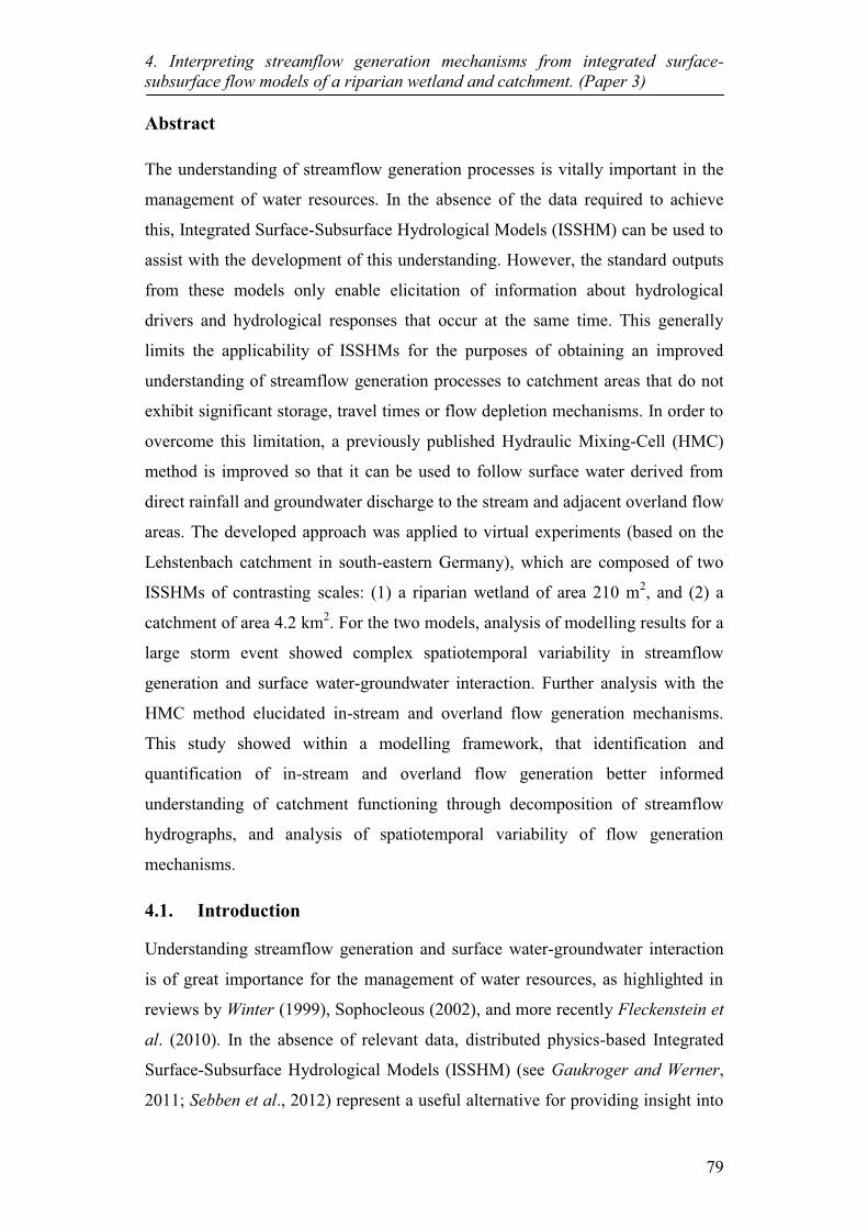
4. Interpreting streamflow generation mechanisms from integrated surface-subsurface flow models of a riparian wetland and catchment. (Paper 3)
79
Abstract
The understanding of streamflow generation processes is vitally important in the
management of water resources. In the absence of the data required to achieve
this, Integrated Surface-Subsurface Hydrological Models (ISSHM) can be used to
assist with the development of this understanding. However, the standard outputs
from these models only enable elicitation of information about hydrological
drivers and hydrological responses that occur at the same time. This generally
limits the applicability of ISSHMs for the purposes of obtaining an improved
understanding of streamflow generation processes to catchment areas that do not
exhibit significant storage, travel times or flow depletion mechanisms. In order to
overcome this limitation, a previously published Hydraulic Mixing-Cell (HMC)
method is improved so that it can be used to follow surface water derived from
direct rainfall and groundwater discharge to the stream and adjacent overland flow
areas. The developed approach was applied to virtual experiments (based on the
Lehstenbach catchment in south-eastern Germany), which are composed of two
ISSHMs of contrasting scales: (1) a riparian wetland of area 210 m2, and (2) a
catchment of area 4.2 km2. For the two models, analysis of modelling results for a
large storm event showed complex spatiotemporal variability in streamflow
generation and surface water-groundwater interaction. Further analysis with the
HMC method elucidated in-stream and overland flow generation mechanisms.
This study showed within a modelling framework, that identification and
quantification of in-stream and overland flow generation better informed
understanding of catchment functioning through decomposition of streamflow
hydrographs, and analysis of spatiotemporal variability of flow generation
mechanisms.
4.1. Introduction
Understanding streamflow generation and surface water-groundwater interaction
is of great importance for the management of water resources, as highlighted in
reviews by Winter (1999), Sophocleous (2002), and more recently Fleckenstein et
al. (2010). In the absence of relevant data, distributed physics-based Integrated
Surface-Subsurface Hydrological Models (ISSHM) (see Gaukroger and Werner,
2011; Sebben et al., 2012) represent a useful alternative for providing insight into

4. Interpreting streamflow generation mechanisms from integrated surface-subsurface flow models of a riparian wetland and catchment. (Paper 3)
80
hydrological processes at detailed spatiotemporal resolutions (e.g. Mirus et al.,
2011b). This is because ISSHMs are capable of simulating feedbacks between the
surface and subsurface, including all forms of overland flow generation and re-
infiltration (Kampf and Burges, 2007). In addition, ISSHMs can assist with
analysing and interpreting hydrological processes and in developing conceptual
understanding of catchment processes (Ebel and Loague, 2006). ISSHM examples
include HydroGeoSphere (Therrien et al., 2009), InHM (Vanderkwaak, 1999),
ParFLOW (Kollet and Maxwell, 2006), CATHY (Camporese et al., 2010) and
MODHMS (HydroGeoLogic Inc., 2006). In recent years, studies related to
understanding streamflow generation and surface water-groundwater interaction
using numerical models have become increasingly widespread (e.g., Brunner et
al., 2009; Frei et al., 2010; Maxwell and Kollet, 2008; Park et al., 2011).
The aforementioned studies focused on processes in small-scale synthetic
systems, enabling insight to be gained into the controls on flow generation (Frei et
al., 2010; Maxwell and Kollet, 2008; Park et al., 2011) and depletion (Brunner et
al., 2009). However, difficulties arise when attempting to gain the same level of
insight for larger, catchment-scale systems. This is because in small-scale
systems, hydrological outputs at a particular place and time are generally only
affected by hydrological drivers that occur at the same location and at the same
time (i.e. by ‘active’ processes (Ambroise, 2004)). However, this is not the case
for larger-scale systems, where local hydrologic response is not only affected by
local processes but largely by processes taking place in other locations and at
other times. This is a result of the influence of surface and groundwater flow
travel times, flow impediments (e.g. riparian wetlands or weirs), and losses (e.g.
infiltration or evaporation). Consequently, hydrological drivers that occur at a
particular point in time (active processes) do not necessarily end up contributing
to the hydrological output at that or a later time. As a result, when considering
streamflow generation processes at the catchment scale, there is a need to
distinguish between ‘active’ and ‘contributing’ processes (Ambroise, 2004), where
contributing processes are those that contribute to flow at a particular location at a
particular time, and necessarily include active processes upstream of the point of
interest. It follows therefore, that all contributing processes are derived from
active processes, occurring both upstream and at the point of interest; however,

4. Interpreting streamflow generation mechanisms from integrated surface-subsurface flow models of a riparian wetland and catchment. (Paper 3)
81
not all active processes will become contributing processes downstream of where
they occur, due to flow depletion processes such as evapotranspiration, and
infiltration to the subsurface. This distinction is particularly important in
catchments with relatively long travel times for water and/or where flow depletion
processes are significant.
While information on active processes is provided as standard output from
ISSHMs, the same is not the case for information on contributing processes. For
example, the lag-times between individual recharge events and resulting stream
flow increases are not reported. As a result, previous studies that have used
ISSHMs at the catchment scale (e.g. Goderniaux et al., 2009; Goderniaux et al.,
2011; Loague and Vanderkwaak, 2002; Ebel et al., 2008; Li et al., 2008; Shen and
Phanikumar, 2010; Mirus et al., 2011a; Camporese et al., 2010) have been unable
to identify and quantify the individual contributions of various catchment
processes to streamflow generation processes. Although Vivoni et al. (2007)
quantified the contributing processes of streamflow generation at the catchment
scale, their model was based on a number of simplifying assumptions that did not
necessitate the distinction between active and contributing processes. In
particular, they assumed that surface water flows to the catchment outlet without
loss or impediment once it enters the surface domain (see Ivanov et al., 2004).
This assumption is problematic in more complex systems where significant
fractions of overland and in-stream flows are depleted (e.g. due to reinfiltration of
overland flow on the hillslope, or losing sections along a stream) or retained in
particular parts of the catchment (e.g. due to wetlands, weirs or other flow
impediments and water storages).
In order to enable ISSHMs to be used for the identification of both active and
contributing streamflow generating processes, it is necessary to first classify water
as it enters the surface by the active flow generation mechanism, and then track
that water on its journey through the catchment, to the point at which the
hydrograph is being measured. Partington et al. (2011, 2012) and Li et al. (2013)
achieved this by developing and applying a Hydraulic Mixing-Cell (HMC)
method in order to identify the groundwater discharge components of hydrographs
for a relatively flat synthetic catchment that exhibited dynamic gaining and losing
reaches along the stream, and furthermore displayed clear time lags for flow from

4. Interpreting streamflow generation mechanisms from integrated surface-subsurface flow models of a riparian wetland and catchment. (Paper 3)
82
upstream areas. However, this approach has not yet been applied to larger-scale
catchments, or for the identification of overland flow generation mechanisms.
In this paper, the HMC method introduced by Partington et al. (2011) is modified
to enable information about active and contributing processes to be obtained as
outputs from ISSHMs. This enables the identification and quantification of
contributing in-stream and overland flow generation mechanisms at larger (e.g.
catchment) scales which informs the understanding of catchment functioning.
This is particularly important as there are still difficulties in the capability to
conduct or scale up the measurements of active processes that are required in
order to gain an understanding of surface water-groundwater interactions and
streamflow generation at the catchment scale (Fleckenstein et al., 2010). The
Lehstenbach catchment is used as the basis for virtual experiments with the
modified HMC method. Two models of contrasting scales are used to investigate
both in-stream and overland flow generation mechanisms within the catchment.
In-stream flow generation mechanisms are defined as those occurring on the
boundaries of the stream, i.e. direct precipitation to the stream, direct groundwater
discharge to the stream and overland flow into the stream. Overland flow
generation is distinguished by rainfall runoff from the hillslope (without
distinguishing infiltration-excess and saturation-excess) and groundwater
discharge on the hillslope adjacent to the stream. Using the HMC method, this
paper aims to demonstrate the value of quantifying in-stream and overland flow
generation mechanisms to better understand processes at the catchment scale
within the virtual experiments by:
1. Separating flow hydrographs into the constituent in-stream and overland
flow generation mechanisms at the outlet and other select points;
2. Quantifying the spatial and temporal variability for in-stream and overland
flow generation mechanisms at contrasting spatial (wetland 210 m2 and
catchment 4.2 km2) and temporal (days vs. year) scales; and
3. Quantifying the differences between active and contributing processes
within the catchment.
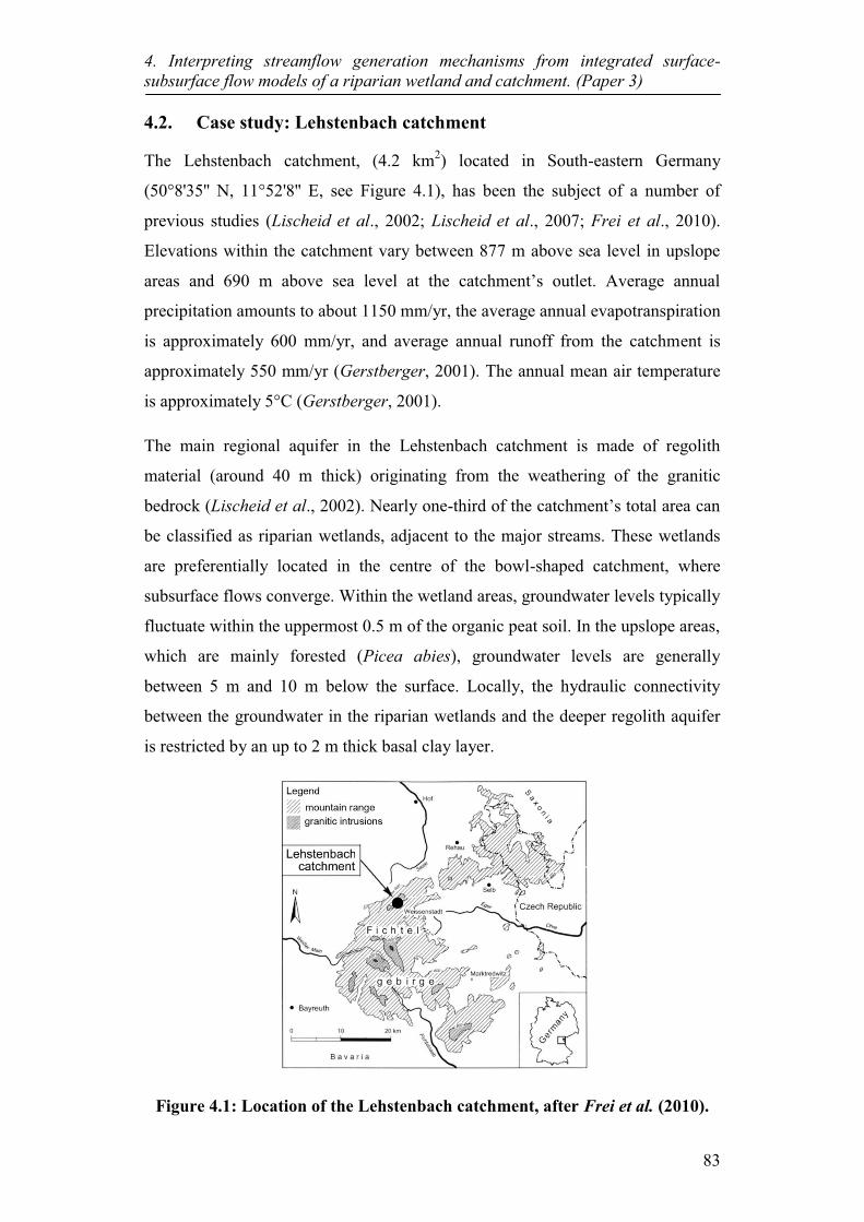
4. Interpreting streamflow generation mechanisms from integrated surface-subsurface flow models of a riparian wetland and catchment. (Paper 3)
83
4.2. Case study: Lehstenbach catchment
The Lehstenbach catchment, (4.2 km2) located in South-eastern Germany
(50°8'35'' N, 11°52'8'' E, see Figure 4.1), has been the subject of a number of
previous studies (Lischeid et al., 2002; Lischeid et al., 2007; Frei et al., 2010).
Elevations within the catchment vary between 877 m above sea level in upslope
areas and 690 m above sea level at the catchment’s outlet. Average annual
precipitation amounts to about 1150 mm/yr, the average annual evapotranspiration
is approximately 600 mm/yr, and average annual runoff from the catchment is
approximately 550 mm/yr (Gerstberger, 2001). The annual mean air temperature
is approximately 5°C (Gerstberger, 2001).
The main regional aquifer in the Lehstenbach catchment is made of regolith
material (around 40 m thick) originating from the weathering of the granitic
bedrock (Lischeid et al., 2002). Nearly one-third of the catchment’s total area can
be classified as riparian wetlands, adjacent to the major streams. These wetlands
are preferentially located in the centre of the bowl-shaped catchment, where
subsurface flows converge. Within the wetland areas, groundwater levels typically
fluctuate within the uppermost 0.5 m of the organic peat soil. In the upslope areas,
which are mainly forested (Picea abies), groundwater levels are generally
between 5 m and 10 m below the surface. Locally, the hydraulic connectivity
between the groundwater in the riparian wetlands and the deeper regolith aquifer
is restricted by an up to 2 m thick basal clay layer.
Figure 4.1: Location of the Lehstenbach catchment, after Frei et al. (2010).

4. Interpreting streamflow generation mechanisms from integrated surface-subsurface flow models of a riparian wetland and catchment. (Paper 3)
84
Previous studies of the Lehstenbach catchment indicated that the dominant runoff
generation processes (e.g. saturated overland flow and shallow subsurface flow)
during rainfall events take place within the wetland areas (Lischeid et al., 2007;
Frei et al., 2010). Large areas of these wetlands, predominantly located near the
catchment’s outlet, are characterised by a pronounced micro-topography,
consisting of sequences of hollows and hummocks formed by the wetland’s
vegetation (Knorr et al. 2008). A conceptual hillslope plot depicting the in-stream
and overland flow generation mechanisms in the Lehstenbach catchment is shown
in Figure 4.2.
Figure 4.2: Conceptual diagram of in-stream and overland flow generation mechanisms typical of the Lehstenbach catchment during intense storm events. The in-stream and overland flow generation mechanisms shown are groundwater discharge to the channel (GW-CH) and wetland surfaces (GW-WL), direct rainfall to the channel (RF-CH) and wetland surfaces (RF-WL), and runoff from the forest.
Previous modelling by Frei et al. (2010, 2012) has been carried out for a synthetic
riparian wetland typical of those within the Lehstenbach catchment. Frei et al.
(2010) demonstrated a hysteretic relationship between wetland water storage and
channel discharge. They concluded that enhanced mixing between surface and
subsurface water had potential implications for the water quality within the
catchment. However, Frei et al. (2010) did not explore mixing of rainfall and
discharged groundwater at the wetland’s surface, which necessitates quantifying
the different overland surface flow and ponding generation mechanisms. These
complex processes in the wetland suggest an analysis of only the active

4. Interpreting streamflow generation mechanisms from integrated surface-subsurface flow models of a riparian wetland and catchment. (Paper 3)
85
mechanisms is insufficient to quantify the contributing overland flow generation
mechanisms. In the present study, application of the HMC method to the wetland
model expands on the work of Frei et al. (2010), and is used to quantify the
fractions of overland flow that are generated from either rainfall running off the
wetland or groundwater discharging to the wetland. However, their wetland model
does not include the surrounding influences of adjacent wetlands, upslope forested
areas and groundwater flows from upslope and deeper aquifers within the
catchment. To investigate the catchment-scale processes, a model of the entire
Lehstenbach catchment is developed, allowing analysis of in-stream and overland
flow generation across the entire stream network and catchment, as well as
accounting for contributions to the wetlands from deeper groundwater that
originated from upslope areas.
4.3. Methodology
The modelling investigation within the study area is carried out at two different
scales, as mentioned previously. Firstly, the model of a synthetic wetland typical
of those in the Lehstenbach catchment is revisited, following Frei et al. (2010)
(Section 4.3.2.1). Secondly, a model of the entire Lehstenbach catchment is
developed (Section 4.3.2.2). In-stream and overland flow generation is analysed
using an improved HMC method detailed in Section 4.3.3.
4.3.1. The fully integrated modelling platform
Numerical modelling in this study uses the ISSHM HydroGeoSphere (HGS).
HGS is a fully integrated surface-subsurface flow model that incorporates 3D
variably saturated subsurface flow using a modified form of the Richard’s
equation and 2D surface flow using the diffusion wave approximation to the St
Venant equations. Further details of the numerical formulation of HGS can be
found in Therrien et al. (2009) and Brunner and Simmons (2012). The surface and
subsurface are coupled using a first-order exchange coefficient (Liggett et al.,
2012). An important characteristic of fully integrated models such as HGS is that
there is no requirement for a priori assumptions of specific streamflow generation
mechanisms (Mirus et al., 2011a). Consequently, it is necessary to interrogate the
model outputs to characterise the streamflow generation processes that are
predicted by the model.

4. Interpreting streamflow generation mechanisms from integrated surface-subsurface flow models of a riparian wetland and catchment. (Paper 3)
86
4.3.2. Development of case study models
4.3.2.1. Wetland model setup
The wetland model setup is described by Frei et al. (2010), and so only a brief
description is presented here. The wetland model (Figure 4.3) is at the plot scale
(21 m x 10 m), representing a relatively flat hillslope (average slope of 0.03 m/m)
made up of a sequence of hummocks and hollows. The spatial structure of the
micro-topography is represented using geostatistical indicator simulations based
on a Markov Chain model of transitional probabilities (Carle and Fogg, 1996).
The model domain is made up of 10 layers, with a total of 410,832 elements and
210,000 nodes, providing a fine discretisation of 0.1 m in the X, Y and Z
directions. The organic peat is represented as homogeneous and isotropic with a
saturated hydraulic conductivity of 0.2 m/d, a value that is based on a previous
Figure 4.3: Geometry of the wetland segment: a) planar reference model showing the main drainage direction and channel location; b) smoothed realisation of the wetlands’ hummocky micro-topography, with simulation results of developed overland flow in the wetland (after Frei et al. (2010)); c) cross section (Y = 5 m) of the micro-topography model (after Frei et al. (2010)). The division of overland flow into two distinct flow networks (denoted as FN1 and FN2) is shown by the surface flow lines. The model observation points for flow in this study are denoted by the red arrows, which correspond to surface water discharge from the wetlands to the channel from FN1 and FN2, and channel discharge at the outlet of the model.

4. Interpreting streamflow generation mechanisms from integrated surface-subsurface flow models of a riparian wetland and catchment. (Paper 3)
87
modelling study from the field site (Hauck, 1999) and which is in line with values
reported for similar wetlands (Kruse et al., 2008; Schlotzauer and Price, 1999).
Constitutive relationships for unsaturated flow are assumed to follow the van
Genuchten model of the soil-water retention and relative permeability functions
(van Genuchten, 1980). The parameterisation of the van Genuchten model is
based on field measurements from similar wetlands located in Alberta, Canada
(Price et al., 2010). Frei et al. (2010) showed that the pronounced micro-
topography resulted in distinct flow networks in the wetland model as shown in
Figure 3b. The division of two flow networks (denoted as FN1 and FN2) and their
discharge points to the channel are shown in Figure 4.3b.
The simulation period in this study focuses on a large storm event (13th - 21st July,
2001) from the 2000-2001 hydrological year (1/11/2000 – 31/10/2001). The
simulation starts with a recession period (i.e. no rain) lasting 14 days. After day
14, an extended rainfall event occurs. The rainfall event persists for 8 days leading
to the depressions on the slope filling until they spill to the adjacent down-slope
depressions. Details of this ‘fill and spill’ mechanism (after Tromp van-Meerveld
and McDonnell, 2006) and its influence on overland flow are described in Frei et
al. (2010).
4.3.2.2. Catchment model setup
A digital elevation model (DEM) with a spatial resolution of 5 m x 5 m is used to
represent the bowl-shaped topography of the catchment. Vertically, the model is
discretised into two main geological units of variable thickness to represent the
major soil types and subsurface geology of the Lehstenbach catchment. Within the
wetland areas, the upper surface unit (1 m thick) represents the organic peat soils.
This upper unit is represented in the grid by 10 sub-layers of uniform vertical
thickness equal to 0.1 m (see Table 4.1).
For the ten sub-layers, the saturated hydraulic conductivity (Ksat) decays
exponentially with depth to account for effects related to the transmissivity
feedback mechanism, which has been described for peat forming wetlands
[Bishop et al., 2004; Jacks and Norrström, 2004). Values for Ksat for the different
sub-layers ranged between 20 m/d for the uppermost layer (representing fresh and
less compacted organic material) and 8.6x10⁻³ m/d for the basal clay layer, which

4. Interpreting streamflow generation mechanisms from integrated surface-subsurface flow models of a riparian wetland and catchment. (Paper 3)
88
separates the wetlands from the deeper aquifer (Table 4.1). The values for Ksat for
the wetland areas are within the range reported by Jacks and Norrstöm (2001)
who performed slug tests for similar wetlands located in the Luntoma catchment
in South-western Sweden. The lower model unit (20-40 m thick) is represented in
the grid by 10 sub-layers and is used to represent the main regolith aquifer.
Similar to the wetland model, parameters for the soil-water retention functions are
applied uniformly to the upper wetland layers based on field measurements from
similar wetlands in Alberta, Canada (Price et al., 2010). Uniform parameters for
the van Genuchten model as well as for Ksat (0.24 m/d) of the main regolith
aquifer are obtained from a previous calibration of the model to field observations
of aquifer heads and stream discharge at the catchment outlet for the 2000-2001
hydrological year (1/11/2000 – 31/10/2001) (see Werb, 2009).
Horizontally, the model uses a triangular mesh with variable node spacing (Figure
4.4). Nodal spacing in the mesh varies between 10 m in the direct vicinity of the
streams, 30 m within riparian wetlands and 100 m for upslope areas. Within HGS,
the locations of streams develop from flow between the surface and subsurface
and tend to occur at topographical lows. However, the DEM used is too coarse to
resolve differences in elevation between stream channels and the surrounding
areas. Therefore, the elevations of surface nodes which coincide with stream
locations are manually lowered by 1 m to correct for the smoothing of topography
in the coarse DEM. For the subsurface flow domain, the bottom and lateral model
boundaries are set to no flow to represent the contact with the low-permeability
granitic bedrock and because it can be assumed that there is no exchange of
groundwater with areas located outside of the Lehstenbach catchment. For the
surface flow domain, a combination of variable rainfall, interception and
evapotranspiration is applied over the catchment. Interception and
evapotranspiration (Panday and Huyakon, 2004), within HGS, are simulated as
mechanistic processes governed by plant and climatic conditions, as described by
Kristensen and Jensen (1975) and Wigmosta et al. (1994). At the edges of the
surface flow domain, a critical depth boundary is used to simulate surface water
outflow from the model. Manning’s roughness coefficient for the forested upslope
areas are assigned uniformly to 1.9x10⁻⁶ d/m1/3, representing areas of minor

4. Interpreting streamflow generation mechanisms from integrated surface-subsurface flow models of a riparian wetland and catchment. (Paper 3)
89
ground vegetation (Shen and Julien, 1993). Friction slope for the wetlands are set
to 8.1 x 10⁻⁵ d/m1/3, typical for high grass (Shen and Julien, 1993).
Topography and land use for the Lehstenbach catchment are shown in Figure 4.4.
The elemental type distribution shown in Figure 4.4 is used to delineate the
stream, wetlands and forest areas. The detailed micro-topography of the wetland
model cannot be included explicitly at the catchment scale due to computational
constraints. Instead, the rill storage concept is used (see Therrien et al., 2009),
whereby a ponding depth is specified at surface nodes which must be reached
before surface flow is induced. Spatially distributed rill storage height zones are
used to represent the micro-topographically induced threshold-type behaviour of
runoff generation from the wetlands. These storage zones mimic the depression-
storage characteristics and the typical fill and spill mechanisms of the wetlands’
micro-topography. However, the behaviour of the wetlands in the catchment-scale
model (as opposed to the wetland model) is influenced additionally by variable
groundwater heads at the upslope boundaries, which are driven largely by
recharge originating from infiltration in the upslope forested areas. The simulation
period is the hydrological year 2000 (11/1/2000 - 10/31/2001), although a focus is
placed on the large July storm (13th - 21st July, 2001) simulated in the wetland
Figure 4.4: Model spatial discretisation of the Lehstenbach catchment and distribution of the stream, wetland and forest areas (the z-axis is exaggerated by a factor of 5). Model observation points are at locations 1 to 6 and the outlet.

4. Interpreting streamflow generation mechanisms from integrated surface-subsurface flow models of a riparian wetland and catchment. (Paper 3)
90
Table 4.1: Surface and subsurface parameters used in the Lehstenbach catchment model. For a detailed description of all model parameters used in HGS, see Therrien et al. (2009).
A NOTE:
This figure/table/image has been removed to comply with copyright regulations. It is included in the print copy of the thesis held by the University of Adelaide Library.

4. Interpreting streamflow generation mechanisms from integrated surface-subsurface flow models of a riparian wetland and catchment. (Paper 3)
91
model. Note that because the whole year is simulated in the catchment model, day
0 in the wetland model is the same as day 200 in the catchment model. Evaluation
of simulated stream discharge to the observed discharge for the 2001-2005
hydrologic years yields a Nash-Sutcliffe efficiency of 0.51, which is deemed
reasonable for this study.
4.3.3. HMC method
The HMC method developed by Partington et al. (2011) allows separation of the
streamflow hydrograph by the in-stream flow generation mechanisms (i.e.
groundwater discharge to the stream, direct rainfall to the stream, and overland
flow to the stream). The HMC method works by utilising the spatiotemporal
information of active in-stream flow generation mechanisms to obtain the
contributing flow generation mechanisms. The HMC method treats each stream
node in the surface domain of the model as a mixing cell. The method utilises the
nodal fluid mass balance from the ISSHM at each model time-step, to calculate
the fraction of water in each cell that derives from different in-stream flow
generation mechanisms. For example, if a cell has a water volume of 0 units at the
start of the time step and 2 units at the end of the time step, and during that time-
step 1 unit of groundwater discharged into the cell and 1 unit of rainfall fell on the
cell, then the fraction of groundwater discharge and direct rainfall in the cell
would be 0.5. This becomes more complex if there is also outflow from the cell,
because a mixing rule must be chosen for the mixing-cells, which dictates how the
fractions are calculated at the end of each time step. The HMC method uses the
“modified mixing rule”, which simulates a mixing regime between perfect mixing
and piston-flow (see Campana and Simpson, 1984).
Each in-stream flow generation mechanism is assigned a unique fraction f. Over
each time-step of the model simulation, inflowing water into a cell from either the
subsurface (e.g. groundwater discharge) or surface boundary conditions (e.g.
rainfall) is classified by the corresponding unique fraction. The sum of all
fractions in each cell, for an error-free fluid mass balance, is equal to 1. Inflow
from adjacent cells is assigned the fractions from the upstream cell. Partington et
al. (2011) derived an equation for the fraction f for each in-stream flow generation
mechanism k at time N in cell i as:

4. Interpreting streamflow generation mechanisms from integrated surface-subsurface flow models of a riparian wetland and catchment. (Paper 3)
92
Ni
Nkj
n
j
N
NjiNkiN
i
m
j
N
Nij
Ni
NiN
ki V
fVf
V
V
VVf
1)(
11
1)(
111
)(
�
��
���� ��
�
�
�����
�
��
(4.1)
Where there are n sources and m sinks for cell i; fj(k)N-1 denotes fraction k at time
N-1 in the neighbouring cell j, V denotes the volume with the superscript denoting
time state and subscript i denoting the cell, ij denoting volume into cell j from cell
i over the time-step from N-1 to N, and ji denoting volume from neighbour j into i.
To achieve the aims of the current study, some limitations from previous
implementations of the HMC method must be addressed. Firstly, Partington et al.
(2011, 2012) does consider the contributing mechanisms for overland flow, as
groundwater discharge adjacent to the stream was negligible. Secondly,
Partington et al. (2011) notes that the HMC method was only numerically stable
if the ratio of outflow to storage was less than 1, and the fluid mass balance
convergence criterion was very small (<10-10 m3/s). These stability conditions
require very low convergence criterion (<10-10 m3/s) for the solution of the fluid
mass balance equation, and very small time-steps (<100 s), thus increasing
simulation time significantly. Use of the HMC method in this study expands on
previous implementations by: (1) accounting for overland flow generation
mechanisms in the HMC method, (2) modifying the HMC scheme to allow
operation at sub-time-steps of the ISSHM flow solution time-step, and (3)
developing stability handling criteria for HMCs to prevent instabilities from
occurring. Addressing these limitations enables the quantification of contributing
in-stream and overland flow generation mechanisms for the more complex virtual
experiment considered in this current study.
4.3.3.1. Capturing in-stream and overland flow generation mechanisms
Overland flow generation mechanisms are considered by using additional HMC
fractions to those used in Partington et al. (2011, 2012). All in-stream and
overland flow generation mechanisms are delineated by surface node definition:
e.g. ‘stream’ or ‘overland’. Surface nodes may also be defined as ‘other’ nodes,
which could be lakes, reservoirs, upstream inflow boundaries or areas for which
internal flow generation may not be of interest or are not known. In this study,
forested areas are treated as ‘other’ nodes. With respect to groundwater discharge

4. Interpreting streamflow generation mechanisms from integrated surface-subsurface flow models of a riparian wetland and catchment. (Paper 3)
93
and rainfall, flow generation at ‘other’ nodes is not captured explicitly. Instead,
any water flowing from ‘other’ nodes to a stream or overland node is assigned an
‘other’ fraction of 1 (i.e. fother = 1), i.e. without delineation of this water into
components of groundwater discharge and rainfall. Unless water in the surface
domain at the start of a simulation is assigned stream, overland or ‘other’ fractions
from a previous simulation, then it is not possible to know which flow generation
processes were responsible for initial surface water. Therefore, an “initial”
fraction is also included; initial conditions for existing surface water in each cell
default to the “initial” fraction (i.e. finitial = 1, and all other fractions are set to zero)
unless predefined otherwise.
4.3.3.2. Sub-timed HMC algorithm to ensure stability
The stability of Eq. 4.1 in the HMC method is dependent on the ratio of outflow to
storage (Partington et al., 2011). ]. Stability requires that the volume of water
leaving a cell over a given time step is less than the volume in storage. The
volume leaving a cell is calculated using the fluid mass balance, accounting for
small errors in the water balance (i.e. ∑ fi(k)N ≠ 1) within each cell (for outflow and
storage). Absolute error (ϵ) within cells is calculated as ϵ = |1-∑ fi(k)N|. The HMC
ratio for each cell i is defined as:
��
�
��
�
��
�
k
Nki
Ni
Nki
m
j
N
Nij
fV
fViratioHMC 1
)(1
1)(
11
)(
(4.2)
Instability in the HMC method results when the cell ratio is greater than 1 in any
HMC. For small HMCs, the storage volume may be quite small relative to the
outflow. Maintaining the HMC ratio below 1 can necessitate very small time-steps
when the cell’s storage is small relative to the flow. This is problematic for long
term transient simulations requiring large time-steps in the flow solution. As part
of the improved HMC method, a sub-timed HMC method is implemented to
prevent relatively small time-steps. This implementation removes the stability
restriction (i.e. Eq. 4.2) imposed by the HMC method on the maximum time-step
for the HGS flow solution. The sub-timed HMC method is applied when the
maximum HMC ratio at any of the cells is greater than 1. It works by subdividing
the fluxes and storage changes within a time-step. This subdivision between time-

4. Interpreting streamflow generation mechanisms from integrated surface-subsurface flow models of a riparian wetland and catchment. (Paper 3)
94
steps N-1 and N, and calculation of fractions at each sub-time step n is done in the
following way:
(1) Calculate the number of sub-time steps (s) required to ensure stability based
on maximum HMC ratio:
s = [max. HMC ratio| + 1 (4.3)
Where max. HMC ratio is the maximum HMC ratio.
(2) Calculate the sub-timed-ratios (tsub) for adjusting inflows, outflows and storage
changes at each n:
���
���
������
�snst
snst
sub
nsub ;)1(*1
1;)1/(11
(4.4)
(3) Calculate the changes in storage for the cells over the whole time-step:
1��� N
iN
ii VVdS (4.5)
(4) Calculate the sub-timed HMC fractions, updating for all cells i at each sub-
step n as follows:
sn
V
tfVf
V
tV
VV
f ni
nsub
nkj
n
j
N
Njinkin
i
nsub
m
j
N
Nij
ni
nin
ki ,...,1,** 1
)(1
11)(
111
)( ��
�
�����
�
��
�
��
���� ��
(4.6)
Subject to
jiaffandVV Nkaka
Nii ,,1
)(0
)(10 ��� �� (4.7)
snfordStnVV in
subN
in
i ���� � 1**1 (4.8)
N
is
i VV � (4.9)

4. Interpreting streamflow generation mechanisms from integrated surface-subsurface flow models of a riparian wetland and catchment. (Paper 3)
95
4.3.3.3. Stability constraints for efficient execution of the HMC method
The sub-timed HMC scheme allows time-steps in the flow solution to be as large
as convergence criteria allow. However, a very large HMC ratio (> 10000), results
in a large number of sub-time steps. In terms of computational efficiency, a very
large HMC ratio is not desirable, particularly for cells that only have very small
volumes of water storage. In near dry cells, large HMC ratios will often arise at
the onset of rainfall, groundwater discharge or overland flow, as the outflow can
be significantly larger than storage. The large HMC ratio problem tends to occur
in simulating ephemeral reaches of streams whereby particular stream cells
become dry. Similarly, this problem occurs in simulating overland flow whereby
the overland cells are often dry (due to overland flow only normally occurring in
rainfall events). In these cases of a large HMC ratio, particular cells can become
numerically unstable due to propagation of errors from the fluid mass balance.
Fortunately, this occurs at cells that are of little interest in a physical sense (i.e.
where active processes take place but with relatively insignificant volumes of
water).
To address these problems and ensure stability and computational efficiency,
criteria are added to the method and used to determine if each cell should be
evaluated. If any of the above criteria are met, then the cell being evaluated is
reset, which means that all fractions f in the reset cell are set equal to zero, and
that the cell is assigned the reset fraction (fReset = 1). The criteria (a-e) for a reset
cell are checked at each time-step allowing it to become active if the reset criteria
are no longer met. The reset fraction allows the tracking of the fraction of water
for which the flow generation is unknown (due to the cell being reset), which
quantifies the effect of the reset fraction. Tracking of the reset fraction highlights
through inspection of calculated HMC fractions if this unknown flow generation
is significant. If the reset fraction of flow in the streamflow hydrograph is high
(>1%) then each criterion can be modified to bring this to a satisfactory level
(<1%).The reset criteria are as follows:
a) Minimum volume. Cells with relatively small water storages are reset
unless surface flow is greater than zero (10-10 in this study).

4. Interpreting streamflow generation mechanisms from integrated surface-subsurface flow models of a riparian wetland and catchment. (Paper 3)
96
b) Ponding only. Cells with no surface flow are reset if the inflow or outflow
is greater than the volume of ponded water.
c) Maximum HMC ratio. Cells with a large HMC ratio (Eq. 4.2) are reset
(104 in this study).
d) Relative volume error too high. Cells in which the ratio of the ‘absolute
volume error’ to storage is large are reset, where the absolute volume error
denotes the absolute value of the error in the volumetric cell balance (2.5
in this study).
e) Error in HMC excessive. Cells with a large absolute error (ϵ) are reset after
updating the fractions in the cell at each time-step or sub-time-step (0.5 in
this study).
4.4. Flow generation analyses conducted using the HMC method
The in-stream and overland flow generation mechanisms analysed for the case
study (see Figure 4.2) are: (1) groundwater discharge to the stream channel (GW-
CH), (2) direct rainfall to the stream channel (RF-CH) and overland flow to the
stream channel. The overland flow generation mechanisms analysed are: (3)
groundwater discharge to wetland surface areas (GW-WL), (4) direct rainfall on
wetlands surface (RF-WL) and (5) overland flow from forested areas (Forest).
The unique fractions f used in this HMC analysis are: (1) GW-CH, (2) RF-CH, (3)
GW-WL, (4) RF-WL, (5) Forest, and also (6) initial water (Initial) and (7) reset
water (Reset). In-stream and overland flow generation mechanisms are
determined based on surface cell type: i.e. stream, wetland or forest cells. Each
analysis outlined below corresponds directly to aims 1 to 3. To aid the reader
through the following sections, Table 4.2 below summarises the flow generation
mechanisms analysed, and the corresponding unique HMC fractions and fraction
types.

4. Interpreting streamflow generation mechanisms from integrated surface-subsurface flow models of a riparian wetland and catchment. (Paper 3)
97
Table 4.2: Considered flow generation mechanisms, HMC unique fractions, and HMC fraction types.
Flow generation mechanism Unique
fraction
Fraction
type
Groundwater discharge to the stream channel GW-CH In-stream
Direct rainfall to the stream channel RF-CH In-stream
Groundwater discharge to the wetlands GW-WL Overland
Direct rainfall to the wetlands RF-WL Overland
Surface flow from the forest area Forest Other
Unknown Initial Initial
- Reset Stability
4.4.1. Separating flow hydrographs by in-stream and overland flow generation mechanisms
The main output from the HMC method is the values of the unique fractions f at
each cell, which are used to separate the flow hydrographs by multiplying the total
flow at each time step by each of the unique fractions at the corresponding time
step. Each flow hydrograph at the outlet and selected model observation points
(see Figure 4.3 and Figure 4.4) is made up of a collection of cells. At each cell,
the surface outflow is separated by the unique fractions into the corresponding
flow generation mechanisms, and then these are summed for each collection of
cells.
4.4.2. Analysing spatiotemporal variability of in-stream and overland flow generation
Spatial variability of in-stream and overland flow in both models is demonstrated
in three ways. Firstly, visualisation of the HMC fractions across the model surface
domain is shown in each model at different points in time. Secondly, flow
hydrographs are shown at select observation points within each of the models.
Lastly, the different flow generation mechanisms driving total flow at each of the
locations are summarised. The summarising of the flow components is achieved
by integrating over the flow curves for each of the flow generation mechanisms, at
each selected observation point.

4. Interpreting streamflow generation mechanisms from integrated surface-subsurface flow models of a riparian wetland and catchment. (Paper 3)
98
4.4.3. Analysing active and contributing processes
The analysis of active and contributing processes is carried out over the entire
year long simulation for the catchment scale model. In particular, the components
analysed are GW-CH, RF-CH and wetlands surface discharge to the stream
channel (WL-CH = GW-WL + RF-WL). Runoff from the forested areas to the
stream channel is also considered (Forest-CH). The active flow generation
processes are determined by summing the inflowing fluxes to the surface domain
(GW-CH, RF-CH, WL-CH, Forest-CH) at each time-step, and the contributing
processes (taken at the outlet) are determined from the HMC analysis. A long-
term ratio of contributing to active flow generation mechanisms is calculated to
quantify the cumulative difference between these two.
4.5. Results and discussion
4.5.1. Wetland model
4.5.1.1. In-stream and overland flow generation mechanisms driving flow
The applied rainfall and the resultant outflow and corresponding flow generation
components are shown in Figure 4.5a-b. From the time rainfall starts, streamflow
increases slightly until day 17, at which point the rainfall rate increases
significantly. The rain falling directly on the channel contributes to runoff
immediately. The infiltration across the overland area increases the subsurface
head, which in turn increases the groundwater discharge to the channel. The rapid
response of rainfall directly on the channel (RF-CH) is clearly seen to follow the
pattern of the rainfall input. During the highest rainfall period, over day 17, the
groundwater discharge to the channel rises to an apparent quasi-steady-state. In
the four days that follow, the GW-CH component only changes slightly in relation
to the total streamflow. All major changes in streamflow between days 17 to 22
are attributed to changes in overland flow to the stream. It can be seen in Figure
4.5c that at approximately 17.6 days, overland flow from FN1 reaches the channel
and causes a rapid increase in streamflow.

4. Interpreting streamflow generation mechanisms from integrated surface-subsurface flow models of a riparian wetland and catchment. (Paper 3)
99
Figure 4.5: Hyetograph, simulated outlet hydrograph, simulated FN1 hydrograph, simulated FN2 hydrograph and simulated surface water storage graph for the wetland model during a large storm event. GW-CH and RF-CH are direct groundwater discharge and rainfall to the channel. GW-WL and RF-WL represent groundwater discharge and rainfall to the surface of the wetland area respectively. Initial represents the initial water in the surface domain at the beginning of the simulation. The reset fraction of flow was negligible and hence is not shown.
Figure 4.5d shows that almost half a day after FN1 starts discharging to the
channel, at approximately day 18, FN2 starts contributing to streamflow. Whilst a
greater proportion of rainfall to the wetland surface area (RF-WL) is evident, there
is also a large component of groundwater that discharged to the wetland surface
(GW-WL). This large component of GW-WL in the outflow hydrograph appears
not only to be an increase in this overland flow generation mechanism at this
particular time, but also a result of the mobilisation of the ponded water generated

4. Interpreting streamflow generation mechanisms from integrated surface-subsurface flow models of a riparian wetland and catchment. (Paper 3)
100
from GW-WL. The total surface water storage across the model and also the flow
generation mechanisms that created the storage are shown in Figure 4.5e. The
ponding of water in the hollows makes up almost 100% of the surface storage
(with the GW-CH and RF-CH water being relatively insignificant). There is only
a relatively small variation in the total storage after day 18. A small component of
initial water is contributing to streamflow at the outlet at day 18. The initial water
was mobilised after the hollows fill and then spill toward the stream. This shows a
slow rate of turnover (>18 d) of ponded surface water due to the time taken for the
hollows to ‘fill and spill’, i.e. prior to the activation of the flow networks.
4.5.1.2. Spatiotemporal variability of in-stream and overland flow generation
Two snapshots of in-stream and overland flow generation are shown for the
wetland model, just before the rainfall event at the start of day14 (Figure 4.6), and
6 days into the storm event at day 20 (Figure 4.7). The distributions of (1) GW-
WL water in the hollows, and (2) GW-CH water, are shown in Figure 4.6 and
Figure 4.7. After 14 days, the rainfall event begins and therefore there is no RF-
CH or RF-WL fraction of surface water (not shown in Figure 4.6). The reason that
the fraction of GW-WL water is not equal to 1 across the hummocks and hollows
is because of the persistence of initial water, of which a small volume resides on
the surface.
The development of overland flow in the wetlands is well established at day 20.
An increase in the GW-WL component of streamflow is explained by the
increased subsurface heads leading to a more developed seepage face along the
bank. Close examination of the two flow networks (FN1 and FN2) highlights
variations in the overland flow generation across the wetland. The overland flow
network on the left (FN1) has a slightly higher component of groundwater
discharge, whereas the flow network on the right (FN2) has a slightly higher
component of rainfall, with clear spatial variation in each. The flow network FN2
has a higher rainfall driven component because of the larger surface area of the
stored water, which receives more rainfall. The reset of cells at the top of the
hummocks and the upper part of the stream bank is due to the fact that these cells
have no surface flow to other cells and also the inflow from rainfall at these cells
is much greater than the ponded water volume.

4. Interpreting streamflow generation mechanisms from integrated surface-subsurface flow models of a riparian wetland and catchment. (Paper 3)
101
Figure 4.6: Wetland HMC fractions at day 14 (pre-storm event). The in-stream and overland flow generating mechanisms shown are: a) groundwater discharge to the channel (GW-CH), b) groundwater discharge to the wetland surface (GW-WL). The initial and reset fractions are also shown in c) and d) respectively. A GW-WL fraction of 0.5 denotes that 50% of the water at that cell was generated from groundwater discharging to the wetland surface.
Figure 4.8 shows a summary of the percentage of total volume of water derived
from different in-stream and overland flow generation mechanisms. This
summary is provided at the outlet and for each of the flow networks (FN1 and
FN2). All volumes were determined by integrating over the flow hydrographs in
Figure 4.5 (b-d). The contributions towards total flow from the two overland flow
networks were calculated to be 34% and 10% for FN1 and FN2, respectively,
making a total overland flow contribution of 44% over the simulation period. The
components of initial water and reset water, are insignificant (<1%). The volume
attributed to cumulative error was extremely small at the outlet (4 x 10-16%).
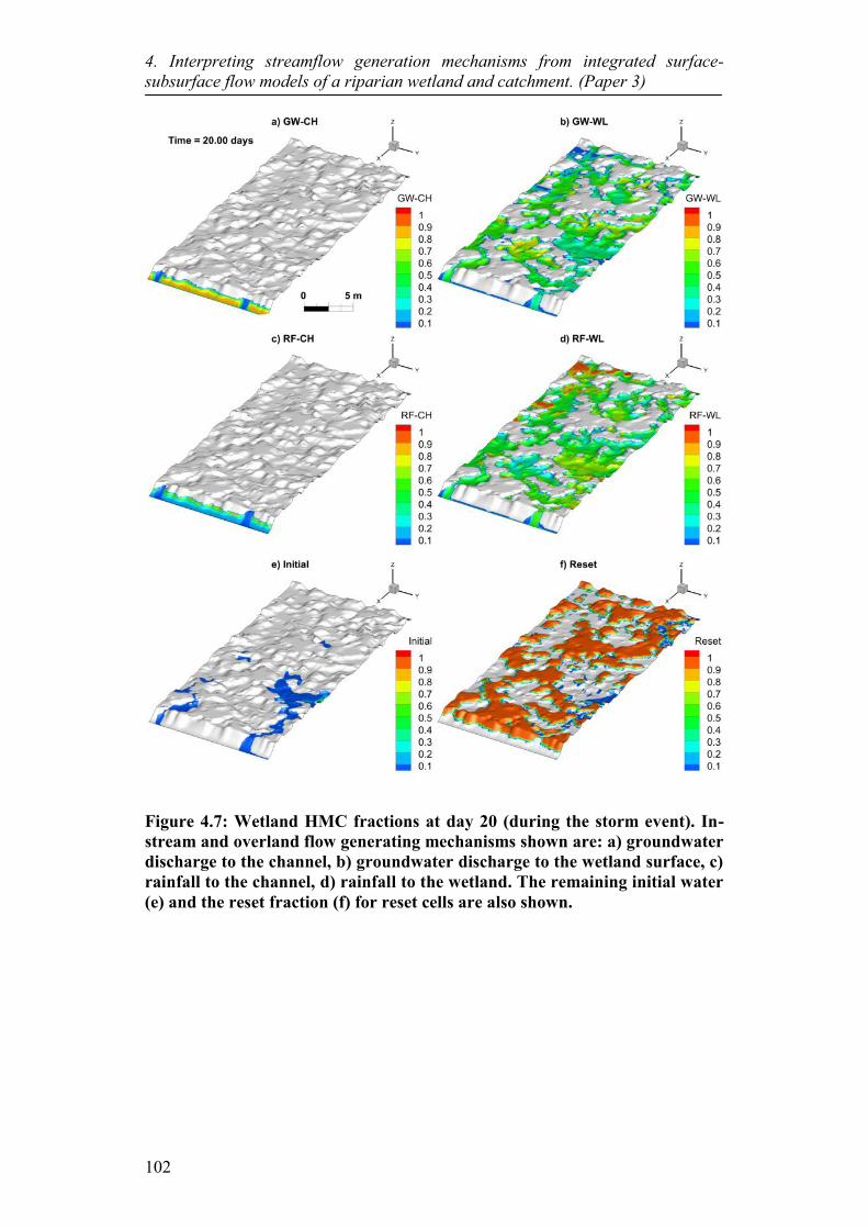
4. Interpreting streamflow generation mechanisms from integrated surface-subsurface flow models of a riparian wetland and catchment. (Paper 3)
102
Figure 4.7: Wetland HMC fractions at day 20 (during the storm event). In-stream and overland flow generating mechanisms shown are: a) groundwater discharge to the channel, b) groundwater discharge to the wetland surface, c) rainfall to the channel, d) rainfall to the wetland. The remaining initial water (e) and the reset fraction (f) for reset cells are also shown.

4. Interpreting streamflow generation mechanisms from integrated surface-subsurface flow models of a riparian wetland and catchment. (Paper 3)
103
Figure 4.8: Comparison of different streamflow generation mechanism contributions at the outlet, FN1 and FN2. The initial and reset fractions and the cumulative error in the cells were insignificant, as can be seen at the top of the stacked columns.
To summarise, HMC analysis of the wetland model demonstrates clear spatial
variability in overland flow generation, as depicted in Figure 4.6 and Figure 4.7.
This variability is clear in the discharge hydrographs of the two flow networks
(Figure 4.5), highlighting a complex relationship between rainfall input and runoff
from the wetlands into the stream. However, despite this spatial variability, the
flow networks have similar compositions of overland flow generation components
at the point of discharge into the stream, with both FN1 and FN2 being dominated
by RF-WL flow generation (Figure 4.8). The HMC analysis showed that the RF-
WL component of flow is larger by about 5% over the GW-WL component in
driving the overland flow contribution at the outlet (Figure 4.8). As evidenced in
the Figure 4.5 discharge hydrographs, the storage across the overland area shows
that the relationship between overland storage and overland flow contributions to
streamflow at the outlet is non-linear. As noted in Frei et al. (2010) this non-linear
relationship is caused by the complex nature of the ‘fill and spill’ mechanism. As
expected, the direct RF-CH component of in-stream flow generation followed the
rainfall input. This is because there are no significant time lags or losses along the
stream to the subsurface. Similarly, the response to rainfall of groundwater
discharge in the channel (GW-CH) is also as expected, although it has a slower
response than the RF-CH component.
0% 10% 20% 30% 40% 50%60% 70% 80% 90%
100%
Outlet FN1 FN2
Sum
med
frac
tion
ERROR
RESET
INITIAL
RF-WL
GW-WL
RF-CH
GW-CH

4. Interpreting streamflow generation mechanisms from integrated surface-subsurface flow models of a riparian wetland and catchment. (Paper 3)
104
4.5.2. Catchment model
Three snapshots from the model simulation for the large storm in July 2001 are
examined for surface water distribution and surface-subsurface exchanges. These
snapshots are taken just prior to the storm (day 216), at the peak of the storm (day
218), and 2 days after the peak (day 220). Figure 4.9 shows standard HGS outputs
of surface saturation, exchange flux and depth distribution across the catchment at
each of these times. Figure 4.9a shows that saturation at the surface boundary
increases across the catchment as the storm event progresses.
Figure 4.9: Simulated surface saturation (a), exchange flux (b) and surface water depth (c), prior to the storm, at the storm peak and 2 days after the storm peak. A losing section on the right arm of the stream is highlighted in the third frame of row b). Positive values of exchange flux indicate groundwater discharge to the surface and negative values indicate infiltration of surface water to the subsurface.
The exchange flux (Figure 4.9b) across the catchment shows where water is
exfiltrating from the subsurface to the surface (positive values) and where water is

4. Interpreting streamflow generation mechanisms from integrated surface-subsurface flow models of a riparian wetland and catchment. (Paper 3)
105
infiltrating into the subsurface from the surface (negative numbers). Prior to the
storm event, there is no exchange across the forested areas, water is being lost
from the wetlands to the subsurface, and groundwater is discharging to the stream.
At the peak of the storm, the infiltration rate peaks in the forested areas, but the
infiltration from the wetlands decreases. The area of groundwater discharging to
the stream is slightly increased, but not significantly. At the cessation of the storm
event, the infiltration rate is varied across the forested area. In Figure 4.9b at day
220, about two thirds of the reach on the right arm of the stream is losing
(highlighted by a red ellipse).
The surface water depth distribution (Figure 4.9c) across the catchment highlights
the wetland areas, where most surface ponding occurs. Excluding the stream,
these wetland areas lie at the lowest elevation in the catchment. It is these ponded
wetlands that provide the overland runoff during the storm event. There is
discharge of groundwater at the upper part of the right arm of the stream,
however, this water is returned to the subsurface across the losing stretch of this
reach of the stream (highlighted in Figure 4.9b).
4.5.2.1. In-stream and overland flow generation mechanisms driving flow
The separated streamflow hydrograph at the outlet is shown in Figure 4.10. In
Figure 4.10b, the GW-CH component of streamflow is seen to respond
immediately to rainfall events with no clear lag, possibly due to propagation of a
pressure wave. As rainfall ponds on the hydraulically connected wetlands, this in
turn increases the head in the underlying aquifers. The GW-CH component of
streamflow is seen to make up ~97% of the flow in dry periods – the GW-WL
component of streamflow contributes a very small amount to streamflow during
dry periods (~3%). The RF-WL and GW-WL components of the outlet
hydrograph (Figure 4.10b) show that the wetlands only provide a significant
component to streamflow during the larger storm events (e.g. at the storm peak,
day 218). After the large storm event from day 221, the streamflow is supported
mainly by GW-CH discharge to the stream. Overland flow from the forested areas
had a negligible contribution to overland flow in the wetlands and hence also to
streamflow, and for this reason is not shown in the hydrographs.

4. Interpreting streamflow generation mechanisms from integrated surface-subsurface flow models of a riparian wetland and catchment. (Paper 3)
106
Figure 4.10: Hyetograph (a), separated discharge hydrographs at the outlet (b), as well as the HMC fractions in surface-storage across the catchment (c). Note that overland flow from the forest was negligible (< 0.2%) in contributing to streamflow and so is not shown in (b).
The total surface water storage across the Lehstenbach catchment and the storage
of water from different flow generation mechanisms, i.e. the mechanism by which
the water came into storage are depicted in Figure 4.10c. This figure shows that
much of the storage in the surface is ponded water in the forested areas. The
second largest component of storage is rainfall stored in the wetlands. Notably,
the GW-CH and RF-CH generated surface storages are relatively insignificant
with respect to total storage, yet provide the largest contribution to streamflow.
The surface water volumes of initial, reset and cumulative error are relatively
insignificant (i.e. appear as horizontal lines along y = 0 in the graphs) to the flow
generation mechanisms and are therefore not shown.
4.5.2.2. Spatiotemporal variability of in-stream and overland flow generation
The in-stream and overland flow generation calculated by the HMC method (at
the same snapshot times as in Figure 4.9) for the large July storm are shown in
Figure 4.11. Prior to the storm, at day 216, the GW-CH component of streamflow
over the entire stream is high and dominating. At this time, there are small patches
of RF-CH generated stream water in places where little to no groundwater is
discharging and where there is no upstream flow passing through. A portion of the
wetland areas prior to the storm show GW-WL generated surface storage, a small

4. Interpreting streamflow generation mechanisms from integrated surface-subsurface flow models of a riparian wetland and catchment. (Paper 3)
107
portion of which is feeding into the stream, which is more clearly apparent in the
hydrograph of Figure 4.10. The speckled RF-WL water existing prior to the storm
highlights areas where some ponding from rainfall has occurred that is yet to
either runoff, infiltrate or evaporate. The source of this rain is attributed to smaller
recent rainfall events (not shown). The bottom row of Figure 4.11 shows the
amount of reset (or unknown) fraction across the catchment during the storm.
Areas where the reset fraction is high correspond to areas where either no surface
flow is occurring or ponding is insignificant (as defined in Section 4.3.3.3). This
highlights areas where ponding processes take place, but in such small quantities
of water that they are not of interest, particularly in relation to the streamflow
hydrograph. As noted in Section 4.3.3.3, any reset cell is still tracked, which
means that any surface flow out of a reset cell is also tracked so that the influence
of these cells is accounted for.
At the peak of the large storm, at day 218, the fraction of GW-CH generation
becomes diminished across the stream as rainfall generation mechanisms become
dominant. The reduction of the fraction of GW-CH generation is matched by an
increase in fractions of RF-CH, GW-WL and RF-WL generation. At day 218, an
increase in the active part of the stream on the right arm (including upstream of
the losing section) is shown in the RF-CH generation. The GW-WL generation on
the wetlands at the peak of the storm is reduced. However, it is worth noting that
the GW-WL water appears in the same area as where water has ponded, shown in
the depth distribution in Figure 4.9.
As described in the stability criteria section 4.3.3.3, surface nodes containing less
than 10-10 m3 of water are excluded from analysis and are reset, which causes the
‘speckled’ effect that is seen adjacent to the upper reaches of the stream. This
effect is attributed partly to the spatial variations in rill storage height across the
wetlands. The small water storage at some wetland nodes relates to those wetland
nodes not being saturated and water infiltrating quickly due to the high hydraulic
conductivity near the surface.
4. Interpreting streamflow generation mechanisms from integrated surface-subsurface flow models of a riparian wetland and catchment. (Paper 3)
108
Figure 4.11: HMC calculated in-stream and overland flow generation for the Lehstenbach catchment – before peak (day 216), at peak (day 218) and after the peak (day 220). The flow generation components are: a) groundwater discharge to the channel (GW-CH), b) rainfall to the channel (RF-CH), c) groundwater discharge to the wetlands surfaces (GW-WL), and d) rainfall to the wetlands (RF-WL). The initial fractions are not shown as all initial water has been flushed from the catchment. The reset fractions are shown in row e).

4. Interpreting streamflow generation mechanisms from integrated surface-subsurface flow models of a riparian wetland and catchment. (Paper 3)
109
After the peak of the storm event, at day 220, the GW-CH generation component
starts to increase. This increase is most apparent in the lower reaches of the stream
where the RF-CH generated streamflow has been mostly flushed from the stream.
The RF-CH component is still strong in small isolated areas in upstream parts of
the stream that are not flowing, and instead, are ponding. The wetlands receive
more groundwater discharge after the storm, which is reflected in the extent of
GW-WL generation across the catchment.
Analysis of the entire 2001 hydrological year allowed comparison of the longer
term flow generation across the catchment to the July large storm event. Figure
4.12 shows box plots of the percent contribution of each of the flow generation
mechanisms across the 7 model observation points depicted in Figure 4.4. The left
plot shows the spread for the entire hydrological year and the right shows the
spread for the large July storm (between days 17 and 20). The volume of water
that passed through the outlet and locations 1-6 is determined by integrating over
the streamflow hydrographs for each component of flow and dividing by the total
volume of streamflow that passed through. Not shown are the fractions of ‘forest’
(maximum 0.3%), initial (maximum 0.05%) and reset (maximum 0.41%) and the
cumulative error resulting from imperfect nodal fluid mass balances over the
simulation (maximum -0.9%). These components are relatively insignificant in
comparison to the four main flow generation mechanisms. This volumetric
analysis indicates that the mechanisms for flow generation did not differ
significantly across the Lehstenbach catchment, although greater variation can be
seen across the focused period of the large July storm compared to the entire year.
However, it is worth noting that the ‘outliers’ in the ‘event’ plot correspond to
observation point 1, which contributes less than 1% of the flow over this event.
Comparison of the distribution of individual flow generation processes across the
entire hydrological year showed surprising uniformity across the catchment. The
similarities in flow generation processes over the year long time scale at the seven
model observation locations are possibly due to the uniformly applied rainfall
events and the simplified representation of the micro-topography across the
wetlands.
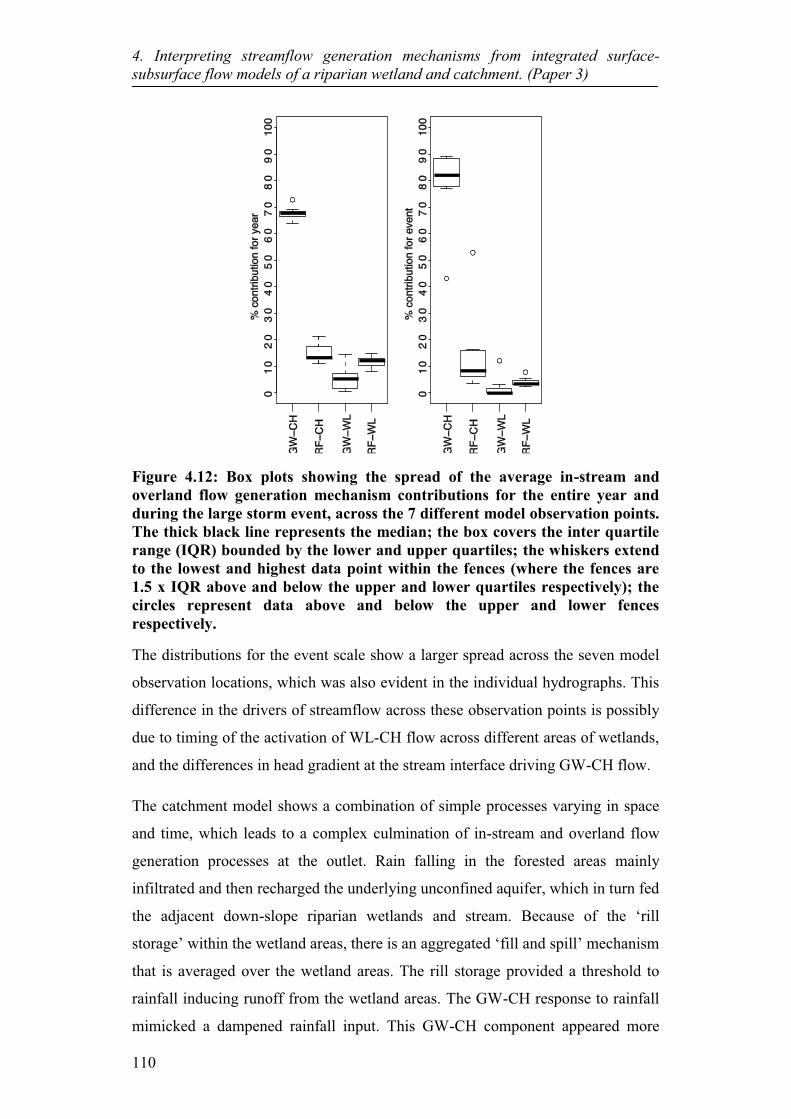
4. Interpreting streamflow generation mechanisms from integrated surface-subsurface flow models of a riparian wetland and catchment. (Paper 3)
110
Figure 4.12: Box plots showing the spread of the average in-stream and overland flow generation mechanism contributions for the entire year and during the large storm event, across the 7 different model observation points. The thick black line represents the median; the box covers the inter quartile range (IQR) bounded by the lower and upper quartiles; the whiskers extend to the lowest and highest data point within the fences (where the fences are 1.5 x IQR above and below the upper and lower quartiles respectively); the circles represent data above and below the upper and lower fences respectively.
The distributions for the event scale show a larger spread across the seven model
observation locations, which was also evident in the individual hydrographs. This
difference in the drivers of streamflow across these observation points is possibly
due to timing of the activation of WL-CH flow across different areas of wetlands,
and the differences in head gradient at the stream interface driving GW-CH flow.
The catchment model shows a combination of simple processes varying in space
and time, which leads to a complex culmination of in-stream and overland flow
generation processes at the outlet. Rain falling in the forested areas mainly
infiltrated and then recharged the underlying unconfined aquifer, which in turn fed
the adjacent down-slope riparian wetlands and stream. Because of the ‘rill
storage’ within the wetland areas, there is an aggregated ‘fill and spill’ mechanism
that is averaged over the wetland areas. The rill storage provided a threshold to
rainfall inducing runoff from the wetland areas. The GW-CH response to rainfall
mimicked a dampened rainfall input. This GW-CH component appeared more
4. Interpreting streamflow generation mechanisms from integrated surface-subsurface flow models of a riparian wetland and catchment. (Paper 3)
111
sensitive than the GW-WL component, which contributed very little to
streamflow. The sensitivity of the GW-CH component is caused by the heads in
the riparian wetlands controlling groundwater flow. As the wetlands and
underlying unconfined aquifer are connected, increases in water levels in the
wetlands from rainfall increases subsurface heads and hence increases the
discharge of groundwater to the stream channel (i.e. GW-CH generation
mechanism). Conversely, the slower, almost filtered response from the GW-WL
generation mechanism is caused by: 1) the time delay in percolation recharging
the unconfined aquifer from the forested areas; then 2) the slow flow of
groundwater through the unconfined aquifers into the wetlands; then 3) the
mobilisation of ponded water in the wetlands into the stream once the wetlands
overtop into the stream.
4.5.2.3. Active versus contributing flow generation mechanisms
A comparison of the active and contributing flow generation processes for GW-
CH, RF-CH and WL-CH is shown in Figure 4.13. In Figure 4.13a, the active
component of GW-CH flow is clearly seen to be higher than the contributing
processes which predominantly results from losing areas along the stream. It
should be noted that the time lags in the stream also lead to a difference between
the active and contributing components, although these are small in this catchment
and hence do not play an obvious role. Similarly in Figure 4.13b and Figure 4.13c
a much larger flux is evident of active RF-CH and WL-CH flow as opposed to the
contributing portion at the outlet. This figure highlights the transient difference
between the active and contributing processes in this catchment.
The long term ratio of contributing to active flow generation processes for WL-
CH (0.78), RF-CH (0.34) and GW-CH (0.25) highlights the significant differences
between active flow generation processes across the catchment and contributing
flow generation processes driving outflow. Furthermore, the cumulative lines
show how this dichotomy develops through time. This supports the need to
differentiate between these active and contributing processes in interpreting
streamflow hydrographs, and therefore, the need to separate the streamflow
hydrograph properly.

4. Interpreting streamflow generation mechanisms from integrated surface-subsurface flow models of a riparian wetland and catchment. (Paper 3)
112
Figure 4.13: Comparison of active and contributing processes with respect to a) GW-CH, b) RF-CH, and c) WL-CH (where WL-CH = RF-WL + GW-WL). Note that the contributing component is superimposed on top of the active component in each of these graphs, i.e. they are not stacked. The long-term ratio of contributing to active processes is also noted in each of the plots, which highlights the average difference between the two. The dashed and dotted lines on each plot represent respectively the cumulative active and contributing components.
4.5.3. Comparison of wetland and catchment models
At the outlet of both models, GW-CH streamflow generation was fairly consistent
across storms with only minor changes relative to the total streamflow
hydrograph. The GW-CH component was seen to respond immediately to rainfall
with no obvious lags in both models. Large changes in streamflow at the outlets
for both models can be attributed to the overtopping of rills within the riparian
wetlands driven by both RF-WL and GW-WL mechanisms. However, in the
catchment model, the RF-CH component contributes significantly to total
streamflow during the large storm event, which is attributable to the coarse model
discretisation of the stream network. This discretisation does not capture the
narrow nature of the actual channels, so that the channels in the model are wider
than they are in reality. The surface area of the stream in the model captures
additional rainfall that would not usually be attributed to the RF-CH flow

4. Interpreting streamflow generation mechanisms from integrated surface-subsurface flow models of a riparian wetland and catchment. (Paper 3)
113
generation mechanism within the catchment. Overland flow from the wetlands in
both models is dominated by RF-WL flow generation. The GW-WL component is
almost as large as the RF-WL component in the wetland model; however, the
GW-WL component is almost negligible at the outlet of the catchment model. The
difference in the GW-WL component between the two models can be attributed to
the discretisation of the wetlands. In the catchment model, the threshold behaviour
to overland flow is captured, which is evident in the wetland model, but the
catchment scale model does not capture the enhanced surface-subsurface mixing
of the wetlands model, which results in a lot of the RF-WL water infiltrating and
then discharging as GW-WL.
4.5.4. Limitations of wetland and catchment models
A number of assumptions were made within this modelling that limited the
representation of reality, as well as any generalisations that can come from it. The
main limitation of the wetland model is that it does not replicate a particular
Lehstenbach wetland, hence there are no observed data to compare with, meaning
the model can only be used for virtual experimentation.
For the catchment scale model, only outflow time series were available for
calibration. As this was the only data used in evaluation of the model, there are
likely to be multiple parameter sets that could yield the same Nash Sutcliffe
efficiency, i.e. equifinality. Alternative parameter sets with equivalent model fits
could potentially lead to significant differences in the spatiotemporal distribution
of flow generation processes and hence influence the dynamics of contributing
processes at the catchment outlet. The resulting non-uniqueness of processes
elicited with the HMC method might not be representative of the actual processes
occurring in the Lehstenbach catchment. This limitation could be addressed (at
least in part) by using additional hydrometric data in model calibrations to further
constrain the problem.
HMC analysis shows that the response of the wetlands in the catchment scale
model seems to be consistent with the understanding of wetland runoff processes
and the catchment behaviour in general; however, the effect of the mesh
discretisation of the stream and wetlands in the catchment model mesh on the
GW-CH response and WL-CH response still requires quantification. Refining the

4. Interpreting streamflow generation mechanisms from integrated surface-subsurface flow models of a riparian wetland and catchment. (Paper 3)
114
coarse mesh would allow for better representation of the enhanced surface-
subsurface mixing, as exhibited in the wetlands scale model, which is important in
consideration of biogeochemical processes (Frei et al., 2012).
The subsurface response is affected by the subsurface boundary conditions, and
no-flow boundaries in the subsurface prevent groundwater from flowing out
through the subsurface, which leads to increased groundwater exfiltration near the
outlet. Although this is generally consistent with the understanding of subsurface
flows in the catchment based on previous studies (Hauck, 1999; Lischeid et al.,
2002), a more thorough assessment of the effects of the subsurface boundary
conditions on catchment outflow would be helpful to further refine our
understanding of the system.
Model simulations would likely have been influenced by: (1) simplification of
heterogeneity within soil types, (2) exclusion of preferential subsurface flow, and
(3) spatiotemporal resolution of rainfall and evapotranspiration inputs (spatially
uniform rather than distributed, daily rather than hourly rainfall and ET). It is
expected that additional heterogeneity (e.g. within each soil layer) would lead to
more complex stream-aquifer exchange patterns, although it is not expected that
this would significantly alter the catchment response. Inclusion of shallow
macropores in the forested areas of the catchment would allow rapid infiltration to
the upper layer of the soil; however, this infiltrated water would be limited in
recharging the aquifer due to the soils’ saturated hydraulic conductivity below the
extent of the macropores. The spatiotemporal resolution of the rainfall and ET
could potentially have a large impact on the catchment response, particularly
where short intense rainfall events lead to flashy streamflow responses, which
would not be captured using the average daily rainfall. With respect to these
assumptions, it is still expected that increased complexity of inputs would lead to
at least the same or greater spatiotemporal variation in the different flow
generation mechanisms. It is not expected that increased complexity would yield
more homogeneous responses in in-stream and overland flow generation
processes, although this is clearly yet to be tested. Furthermore, the influence of
surface flow travel times, flow impediments and flow depletion processes are still
important with respect to spatiotemporal variability of contributing flow
generation processes.

4. Interpreting streamflow generation mechanisms from integrated surface-subsurface flow models of a riparian wetland and catchment. (Paper 3)
115
4.5.5. Evaluation of HMC method implementation
The sub-timed scheme of the HMC method is an important improvement which
allowed application to more complex problems than those studied in Partington et
al. (2011, 2012) and Li et al. (2013). The sub-timed scheme was necessary in both
of the models, significantly reducing the number of flow solution time-steps that
would have been required with the previously developed HMC method (by 106 in
the catchment year long simulation). The sub-timed scheme allowed the adaptive
time-stepping scheme of the flow solution to perform as normal without tight
restrictions on the maximum time-step. Complementary to this improvement, the
stability constraints used in the improved HMC method were able to ensure
stability of the cells in the simulations. The reset fractions resulting from cells that
were reset when they met the criteria outlined in Section 4.3.3.3, highlighted areas
that were of little interest with respect to overland flow generation processes. The
reduction of active cells allowed faster computation and highlighted areas of little
activity with respect to flow generation processes, which is reflected in the spatial
distribution of the reset fraction (Figure 4.6, Figure 4.7 and Figure 4.11) and in the
actual contributing fraction of flow from reset cells.
4.6. Conclusions
In this paper, an improved Hydraulic Mixing-Cell (HMC) method was developed
that enables both active and contributing processes to be obtained from the
outputs of Integrated Surface-Subsurface Hydrological Models (ISSHM), thereby
enabling streamflow generation processes to be identified for catchments that
include significant storage, travel times and losses. Specifically, the following
improvements to the HMC method were made: (1) accounting for overland flow
generation mechanisms, (2) implementing a sub-timed scheme, and (3)
implementing HMC stability constraints.
This improved HMC approach was applied to two virtual experiments based on
the Lestenbach catchment and a wetland typical of the catchment, which enabled
(i) separation of simulated streamflow hydrographs into their constituent in-
stream and overland flow generation mechanisms, (ii) quantification of the spatial
and temporal variability for in-stream and overland flow generation mechanisms
at contrasting spatial and temporal scales, and (iii) quantification of the degree to

4. Interpreting streamflow generation mechanisms from integrated surface-subsurface flow models of a riparian wetland and catchment. (Paper 3)
116
which the active and contributing processes differ within the catchment model,
leading to an improved understanding of simulated streamflow generation
processes. The application of the HMC method in this study is a promising first
step in the refinement of the method; however, as discussed in the model
limitations, the catchment model would benefit from some improvements. Further
development of the catchment model by further calibration using additional
hydrometric data will serve to improve the veracity of the model for quantifying
spatiotemporal variability within the Lehstenbach catchment. Furthermore,
investigation into the influence of the no flow subsurface boundary conditions
used and the areal mesh discretisation would also help to make the catchment
model more representative of the Lehstenbach catchment.
Further development of the HMC method is recommended by greater subdivision
of the rainfall driven overland flow generation mechanisms into saturation-excess
and infiltration-excess. It would be extremely useful to also develop an automatic
definition of the stream based on flow depth, velocity and direction. In addition,
the HMC method should be further expanded to track flow in the subsurface,
which would allow tracking of other flow domains, for example, from macropores
and fractures. Extension to the subsurface would also allow identification of the
source areas of groundwater discharging to the surface. The inclusion of time
stamps to the HMC fractions would also improve the HMC method, and allow
analysis into event and pre-event water contributions.
The composition of streamflow with respect to the different surface runoff
generating processes entails important information on runoff processes and
mechanisms during large rainfall events and during dry periods. The methodology
presented here provides a tool to decipher and deconvolute the integrated
streamflow signal using numerical models. This improves assessment of
catchment functioning within the ‘hypothetical reality’ of the model. This is an
important aspect of the HMC method when applied to physically distributed
models that have no a priori assumption of flow generation processes. Use of the
HMC method provides a necessary assessment of whether or not a catchment
model behaves in the way desired, or more importantly, the way the catchment
processes are conceptualised. In that sense, it is useful for a ‘soft calibration’
based on understanding of catchment functioning from field observations. This

4. Interpreting streamflow generation mechanisms from integrated surface-subsurface flow models of a riparian wetland and catchment. (Paper 3)
117
can only serve to strengthen the relatively small arsenal of tools currently
available for analysing catchment models.
Acknowledgements
The authors gratefully acknowledge Pascal Goderniaux and two anonymous
reviewers whose reviews greatly improved the manuscript. The authors also
gratefully acknowledge the assistance of Grace Lin in developing figures for the
manuscript. This work is supported by the Australian Research Council through
its Linkage scheme and the South Australian Department for Water as the industry
partner under grant number LP0668808. Parts of this research were funded by the
Swiss National Foundation, Ambizione grant PZ00P2_126415. The views
expressed in this paper are solely those of the authors.

4. Interpreting streamflow generation mechanisms from integrated surface-subsurface flow models of a riparian wetland and catchment. (Paper 3)
118

5. Thesis Conclusions
119
Chapter 5
5 Thesis Conclusions The streamflow hydrograph entails important information on flow generation
processes during large rainfall events and during dry periods. The streamflow
hydrograph is one of the most important hydrological descriptors available,
containing the pertinent information of flow maxima and the total volume of
water flowing out of a catchment over time. This information is critical for
management of flooding and water resources. The understanding of where stream
water originates from in the hydrosphere and the processes by which it reaches the
stream underpins catchment hydrology. Research to understand these processes is
being increasingly carried out utilising physics-based fully Integrated Surface-
Subsurface Hydrological Models (ISSHM). In the absence of required field data,
such models are necessary for improving our understanding of catchment
hydrological response. To understand the response, it is critical to understand the
nature in which the processes of flow generation across a catchment and at
different periods in time express themselves in the streamflow hydrograph, whilst
accounting for the processes of flow depletion. However, even though detailed
spatiotemporal outputs from ISSHMs have provided some insight into catchment
functioning, the interpretation of all of this information into an understanding of
how all of the flow generation processes across a catchment express themselves in
the streamflow hydrograph has yet to be realised. In a modelling framework, this
research has achieved this through the development and application of a new
method which identifies and quantifies streamflow generation contributions
allowing full deconvolution of the streamflow hydrograph into its constituent
components of streamflow generation.

5. Thesis Conclusions
120
5.1. Research contributions
The overall contribution of this thesis was in improving the interpretation of in-
stream and overland flow generation mechanisms from ISSHMs (Objective 1),
and the applications this allowed (Objectives 2 to 4). The improvements in this
thesis were achieved through development of a new method that enables
identification and quantification of the active and contributing processes from the
outputs of ISSHMs, thereby enabling streamflow generation processes to be
analysed for catchments that include significant storage, travel times and losses.
Use of the HMC method provides a necessary assessment of whether or not a
catchment model behaves in the way desired, or more importantly, the way the
catchment processes are conceptualised. The method can be used for a ‘soft
calibration’ based on understanding of catchment functioning from real
observations. This can only serve to strengthen the relatively small arsenal of
tools currently available for analysing catchment models.
Specifically, in meeting the objectives of this research laid out in the introduction,
the following research contributions were made:
1. A Hydraulic Mixing-Cell method was developed to quantify the
contribution of flow generation mechanisms to streamflow, allowing
separation of the streamflow hydrograph into its constituent flow
generation components (i.e. groundwater discharge and direct rainfall to
the stream, and groundwater discharge and direct rainfall to overland
areas). Because the HMC method tracks the streamflow generation
mechanisms along the stream, temporal and spatial components that affect
these mechanisms can be accounted for. The HMC method correctly
handles dynamic complex flow regimes (rapid changes of gaining stream
to losing stream and vice versa), accounts for storage effects, flow
impediments and the travel times that occur within a catchment. The
method easily handles the dynamic nature of varying flow regimes in large
and complex systems (e.g. the Lehstenbach catchment). The only data
requirements for the HMC method are the fluxes at each cell and surface
water depths, which are part of the flow solution. By using this method,
contributing processes can be identified and quantified. Improved
knowledge of catchment processes as simulated by HydroGeoSphere was
5. Thesis Conclusions
121
obtained through Hydraulic Mixing-Cell analysis, with meaningful
separation of the streamflow hydrograph indicating how overland and in-
stream flow generation processes drive streamflow.
2. A benchmark against which baseflow separation methods can be tested
was developed by simulating flow in a hypothetical V-catchment in HGS
and using the HMC method to provide the baseflow contribution to total
streamflow at the outlet of the catchment. This benchmark was used to
determine the potential error in commonly used automated methods for
estimation of in-stream groundwater contributions to streamflow. The
numerical experiments in this showed that even in the “simple”
hypothetical V-catchment, baseflow dynamics are complex. This
complexity in baseflow dynamics affected the performance of the
commonly used automated separation methods, which resulted in
unsatisfactory performance of each method examined in at least one of the
events and scenarios considered. The potential error was found to be
significant in automated methods for estimating groundwater contributions
to streamflow, and this warrants caution in overvaluing their outputs. It is
perhaps the case that the uncertainty associated with simple automated
methods precludes their use for providing anything more than very rough
estimates of baseflow.
3. The first investigation – using an ISSHM – was conducted into the
spatiotemporal variability in both overland and in-stream flow generation
mechanisms. This was done using two models of a wetland and catchment,
from a case study of a real catchment. The spatiotemporal variability was
analysed through snapshots in time during a large storm event, and
through hydrographs at a number of points within each of the models.
Both models exhibited significant spatial variability in flow generation
processes. In the catchment model, temporal variability of streamflow
generation at a number of locations was seen to be significant over a large
storm, but similarities increased using a longer term annual average of
flow in-stream and overland flow generation processes.
4. The first investigation – using an ISSHM – was conducted into the
dichotomy that exists between ‘active’ and ‘contributing’ streamflow
generation mechanisms within a modelling framework. Differences
5. Thesis Conclusions
122
between the active and contributing processes were quantified by the long
term ratio between active and contributing processes. It was found that
accounting for in-stream and overland losses and in-stream and overland
flow travel time is necessary in accurately quantifying the constituent in-
stream and overland flow generation components of streamflow. It is
therefore recommended to employ the HMC method in ISSHM studies of
various flow generation processes.
5. The HMC method developed in this research was implemented in the HGS
code. This implementation means that all of the analyses conducted in this
research can be carried out in models built in HGS using simple
instructions in the HGS pre-processor.
5.2. Research limitations
Limitations of this research were due to current modelling limitations, scope of
research and time-constraints. The limitations that arose are detailed as follows:
1. Modelling limitations: A main limitation of this research lay within the
ability to run a large number of (tens and hundreds of simulations) or long
term models scenarios (years). This is due to the lengthy model run-times
(of the order of weeks for each simulation in each of the research papers)
that result from solving the highly non-linear partial differential equations
describing flow. A parallel version of HGS has now been developed which
should reduce the model run-times and allow a greater number of
scenarios to be explored in future research. Another limitation associated
with the run-times relates to the accuracy required in the HGS flow
solution in order to ensure stability in the HMC method and also ensure an
acceptable level of error. Despite this being highlighted as a limitation, it
should be noted that it is good modelling practice to ensure tight
convergence criteria, resulting in minimal nodal fluid mass balance errors
as opposed to global mass balance errors.
2. Limitations in investigation of automated baseflow separation methods:
The investigation of commonly used automated baseflow separation
methods was limited by the number of scenarios run and scenario time-
length in the hypothetical catchment used. The shape of the catchment
considered was rectangular, however, effects of convergent and divergent

5. Thesis Conclusions
123
catchment shapes were not considered. The characterisation of physical
parameters within the catchment was relatively simple, without
consideration of multilayered soils or heterogeneous soil properties. The
hydrological forcing was applied in a spatially uniform manner and at a
coarse temporal scale (daily) in these simulations, although these effects
may be important in the catchment response of baseflow generation. This
research focused on commonly used automated methods that rely only on
the streamflow hydrograph for the baseflow separation, however there has
been an emergence of physically based filters (e.g. Furey and Gupta,
2001, 2003; Huyck et al., 2005) which were not considered.
3. Limitations of streamflow generation analysis: The HMC method
developed in this research was used to delineate the direct groundwater
discharge and rainfall to streams and overland areas. A common
consideration of overland flow generation mechanisms not considered in
this research was the rainfall runoff mechanisms of infiltration excess
(Hortonian) and saturation excess (Dunne). These processes were not
considered in the case study of this research, although in most other
catchments, these mechanisms will be of interest. The use of ISSHMs in
building intuition of catchment functioning is highly valuable, although it
is also dependent on the assumptions in the model (even if these are
deemed reasonable). In consideration of streamflow generation
mechanisms, real observation will always be the most important driver for
advancing the science. However, as highlighted throughout this thesis, the
conceptual understanding of streamflow generation processes can be built
from ISSHMs.
5.3. Recommendations for future work
This research has opened up a new way of analysing and interpreting flow
processes using ISSHMs. There are still further applications of the HMC method
that would benefit research utilising ISSHMs and address the limitations
identified above. It is recommended that the HMC method be expanded to
improve analysis and interpretation of subsurface flow processes including flow
through: saturated and unsaturated dual continuum media, fractures, and macro-
pores. Further development of the HMC method is recommended by greater
subdivision of the rainfall driven overland flow generation mechanisms into

5. Thesis Conclusions
124
saturation-excess and infiltration-excess. Extension to the subsurface would also
allow identification of the source areas of groundwater discharging to the surface.
Furthermore, the inclusion of time stamps to the HMC fractions would serve to
improve the HMC method, and allow analysis into event and pre-event water
contributions. Application of the HMC method encompassing all of the above
recommendations would provide a highly comprehensive analysis of catchment
functioning and provide complete analysis of the different aspects of streamflow
generation as shown in Figure 5.1 (adapted from Sklash and Farvolden, 1979).
This research considered the flow generation delivery mechanisms without
distinction of the overland flow generation mechanisms, i.e. infiltration excess
and saturation excess overland flow.
Figure 5.1: Comprehensive conceptualisation of catchment response to rainfall (adapted from Sklash and Farvolden, 1979). The dashed red line indicates the aspects considered in this research, although without distinction of overland rainfall driven mechanisms (i.e. infiltration excess (Hortonian) or saturation excess (Dunne)).
The HMC method presented in this thesis can be applied within any ISSHM, and
as part of this research has been coded into the HGS code to allow other HGS
users the ability to easily utilise it. For example, this HGS implementation has
already been used outside of this research in Sebben (2011) and Li et al. (2012)
and is currently being used in a number of other research projects. It is
recommended that the HMC method be employed in future versions of other
STORM RUNOFF
EVENT
TIME ASPECTS FLOW GENERATION
MECHANISM ASPECTS
SOURCE
ASPECTS
Water added by specific event (event water)
Water in basin prior to specified event (pre-event water)
Infiltration excess overland flow
Saturation excess overland flow
Groundwater discharge to stream
Channel interception
Combination
Groundwater
Direct Rainfall
Vadose Water
Direct Runoff
Combination Groundwater discharge to hillslope

5. Thesis Conclusions
125
ISSHM codes. This is relatively simple as the coding of the HMC method requires
only that all components of the nodal fluid mass balance (inflows, outflows, and
changes in storage) and nodal neighbour relations be output or passable within the
code. The HMC method could be very beneficial in future model inter-
comparison studies to compare the constituent components of the streamflow
hydrograph and spatiotemporal flow generation.
With respect to the application of the HMC method in investigating potential
errors in commonly used automated baseflow separation methods, further work is
required to understand the appropriate use of baseflow separation methods. More
complex baseflow separation methods than those considered in this study should
be tested in future studies. Physically based filters (e.g. Furey and Gupta, 2001,
2003; Huyck et al., 2005) could prove to be more robust. This is because they
provide a physically based relation of rainfall and ET (and other physical
parameters) to baseflow.
In all of the simulations carried out in this research, the characterisation of
hydrological forcing and distribution of catchment characteristics could be
improved. Future studies should aim to elucidate the spatial and temporal scale
dependence of flow generation mechanisms. In the studies using hypothetical
catchments for numerical experimentation, the impact of variations in geology,
topography and vegetation, should be investigated by incrementally adding layers
of complexity to similar models in order to try and understand flow generation
dynamics.

5. Thesis Conclusions
126

References
127
References
Adar, E.M., S.P. Neuman, and D.A. Woolhiser (1988), Estimation of Spatial
Recharge Distribution Using Environmental Isotopes and Hydrochemical Data
.1. Mathematical-Model and Application to Synthetic Data, Journal of
Hydrology, 97:251-277.
Ambroise, B. (2004), Variable ‘active’ versus ‘contributing’ areas or periods: a
necessary distinction, Hydrological Processes, 18: 1149–1155,
doi:10.1002/hyp.5536.
Arnold, J.G., P.M. Allen, R. Muttiah, and G. Bernhardt (1995), Automated Base-
Flow Separation and Recession Analysis Techniques, Ground Water, 33: 1010-
1018.
Arnold, J.G., and P.M. Allen. (1999), Automated methods for estimating baseflow
and ground water recharge from streamflow records, Journal of the American
Water Resources Association, 35: 411-424.
Barnes, B. (1939), The structure of discharge-recession curves, Transaction of the
American Geophysical Union, 20: 721-725.
Becker, M.W., T. Gerogian, H. Ambrose, J. Siniscalchi, K. Frederick (2004),
Estimating flow and flux of ground water discharge using water temperature
and velocity, Journal of Hydrology, 296: 221-233.
Bishop, K., J. Seibert, S. Köhler, and H. Laudon (2004), Resolving the double
paradox of rapidly mobilized old water with highly variable responses in runoff
chemistry, Hydrological Processes, 18: 185–189, doi: 10.1002/hyp.5209.

References
128
Brunner, P., P.G. Cook, and C.T. Simmons (2009a), Hydrogeologic controls on
disconnection between surface water and groundwater, Water Resources
Research, 45, W01422, doi:10.1029/2008WR006953.
Brunner, P., C.T. Simmons, and P.G. Cook (2009b), Spatial and temporal aspects
of the transition from connection to disconnection between rivers, lakes and
groundwater, Journal of Hydrology, 376:159-169.
doi:10.1016/j.jhydrol.2009.07.023.
Brunner, P., and C.T. Simmons (2011), HydeoGeoSphere: A fully integrated
physically based hydrological model, Ground Water, doi:10.1111/j.1745-
6584.2011.00882.x.
Boughton, W.C. (1993), A hydrograph-based model for estimating the water yield
of ungauged catchments, Paper presented at Hydrology and Water Resources
Symposium, Inst. of Eng. Aust., Newcastle, N.S.W.
Brutsaert, W., and J.L. Nieber (1977), Regionalized Drought Flow Hydrographs
from a Mature Glaciated Plateau, Water Resources Research, 13: 637-644.
Campana, M.E., and E.S. Simpson (1984), Groundwater Residence Times and
Recharge Rates Using a Discrete-State Compartment Model and C-14 Data.
Journal of Hydrology, 72:171-185.
Camporese, M., C. Paniconi, M. Putti, and S. Orlandini (2010), Surface-
subsurface flow modeling with path-based runoff routing, boundary condition-
based coupling, and assimilation of multisource observation data, Water
Resources Research, 46, W02512, doi:10.1029/2008WR007536.
Carle, S.F. and G.E. Fogg (1996), Transition Probability-Based Indicator
Geostatistics, Mathematical Geology, 28(4): 453–476,
doi:10.1007/BF02083656.
Carsel, R. F., and R.S. Parrish (1988), Developing Joint Probability-Distributions
of Soil-Water Retention Characteristics, Water Resources Research, 24:755-
769.
Chapman, T. (1991), Evaluation of Automated Techniques for Base-Flow and
Recession Analyses – Comment, Water Resources Research, 27: 1783-1784.

References
129
Chapman, T. (1999), A comparison of algorithms for stream flow recession and
baseflow separation, Hydrological Processes, 13: 701-714.
Chapman, T.G. (2003), Modelling stream recession flows, Environmental
Modelling and Software, 18:683-692.
Chow, V.T. (1959), Open channel hydraulics, McGraw-Hill, New York.
Cook, P.G., G. Favreau, J.C. Dighton and S. Tickell (2003), Determining natural
groundwater influx to a tropical river using radon, chlorofluorocarbons and
ionic environmental tracers, Journal of Hydrology, 277: 74-88.
Cook, P.G., C. Wood, T. White, C.T. Simmons, T. Fass and P. Brunner (2008),
Groundwater inflow to a shallow, poorly-mixed wetland estimated from a mass
blance of radon, Journal of Hydrology, 354: 213-226.
Croton, J.T., and D.A. Barry (2001), WEC-C: a distributed, deterministic
catchment model - theory, formulation and testing, Environmental Modelling
and Software, 16:583-599.
Ebel, B.A. and K. Loague (2006), Physics-based hydrologic-response simulation:
Seeing through the fog of equifinality, Hydrological Processes, 20(13): 2887-
2900, doi:10.1002/hyp.6388.
Ebel, B.A., K. Loague, D.R. Montgomery, and W.E. Dietrich (2008), Physics-
based continuous simulation of long-term near-surface hydrologic response for
the Coos Bay experimental catchment, Water Resources Research, 44,
W07417, doi:10.1029/2007WR006442.
Ebel, B.A., B.B. Mirus, C.S. Heppner, J. E. VanderKwaak, and K. Loague (2009),
First-order exchange coefficient coupling for simulating surface water-
groundwater interactions: parameter sensitivity and consistency with a physics-
based approach, Hydrological Processes, 23:1949-1959.
Eckhardt, K. (2005), How to construct recursive digital filters for baseflow
separation, Hydrological Processes, 19: 507-515.

References
130
Eckhardt, K. (2008), A comparison of baseflow indices, which were calculated
with seven different baseflow separation methods, Journal of Hydrology,
352:168-173.
Facchi, A., B. Ortuani, D. Maggi, and C. Gandolfi. (2004), Coupled SVAT-
groundwater model for water resources simulation in irrigated alluvial plains,
Environmental Modelling and Software, 19:1053-1063.
Fenicia, F., H.H.G. Savenije, P. Matgen, and L. Pfister (2006), Is the groundwater
reservoir linear? Learning from data in hydrological modelling, Hydrology and
Earth Systems Science, 10: 139-150.
Ferket, B.V.A., B. Samain, and V.R.N. Pauwels (2010), Internal validation of
conceptual rainfall-runoff models using baseflow separation, Journal of
Hydrology, 381: 158-173.
Fleckenstein, J.H., S. Krause, D.M. Hannah, and F. Boano (2010), Groundwater-
surface water interactions: New methods and models to improve understanding
of processes and dynamics, Advances in Water Resources, 33(11): 1291-1295.
doi:10.1016/j.advwatres.2010.09.011.
Freeze, R.A. and R.L. Harlan (1969), Blueprint for a physically-based, digitally-
simulated hydrologic response model, Journal of Hydrology, 9:237-258.
Freeze, R.A. (1972), Role of Subsurface Flow in Generating Surface Runoff 1.
Base Flow Contributions to Channel Flow, Water Resources Research, 8: 609-
623.
Frei, S., G. Lischeid, and J.H. Fleckenstein (2010), Effects of micro-topography
on surface-subsurface exchange and runoff generation in a virtual riparian
wetland - A modeling study, Advances in Water Resources, 33(11): 1388-1401,
doi:10.1016/j.advwatres.2010.07.006.
Frei, S., K.H. Knorr, S. Peiffer, and J.H. Fleckenstein (2012), Surface micro-
topography causes hot spots of biogeochemical activity in wetland systems: A
virtual modeling experiment, Journal of Geophysical Research, 117, G00N12,
doi:10.1029/2012JG002012.

References
131
Furey, P.R., and V.K. Gupta (2001), A physically based filter for separating base
flow from streamflow time series, Water Resources Research, 37(11): 2709-
2722.
Furey, P.R., and V.K. Gupta (2003), Tests of two physically based filters for base
flow separation, Water Resources Research, 39(10): 1297.
Gaukroger, A.M., and A.D. Werner (2011), On the Panday and Huyakorn surface-
subsurface hydrology test case: analysis of internal flow dynamics,
Hydrological Processes, 25: 2085-2093.
Gerstberger, P. (2001), Waldökosystemforschung in Nordbayern, Die Bitök-
Untersuchungsflächen im Fichtelgebirge und Steigerwald, in: Bayreuther
Forum Ökologie, edited by: BITÖ K, B. I. f. T. Ö ., BITÖK, Bayreuther
Institut für Terrestrische Ökosystemforschung, Bayreuth, 193 pages.
Gilfedder, M., G.R. Walker, W.R. Dawes, and M.P. Stenson (2009), Prioritisation
approach for estimating the biophysical impacts of land-use change on stream
flow and salt export at a catchment scale, Environmental Modelling and
Software, 24:262-269.
Goderniaux, P., S. Brouyere, H. J. Fowler, S. Blekinsop, R. Therrien, P. Orban,
and A. Dassargues (2009), Large scale surface-subsurface hydrological model
to assess climate change impacts on groundwater reserves, Journal of
Hydrology, 373: 122-138, doi:10.1016/j.jhydrol.2009.04.017.
Goderniaux, P., S. Brouyère, S. Blenkinsop, A. Burton, H. J. Fowler, P. Orban,
and A. Dassargues (2011), Modeling climate change impacts on groundwater
resources using transient stochastic climatic scenarios, Water Resources
Research, 47, W12516, doi:10.1029/2010WR010082.
Gupta, H.V., S. Sorooshian, and P.O. Yapo (1999), Status of automatic calibration
for hydrologic models: Comparison with multilevel expert calibration, Journal
of Hydrologic Engineering, 4: 135-143.

References
132
Halford K.J., and G.C. Mayer (2000), Problems Associated with Estimating
Ground Water Discharge and Recharge from Stream-Discharge Records,
Ground Water, 38: 331-342.
Hall, F.R. (1968), Base-Flow Recessions-a Review, Water Resources Research, 4:
973-983.
Hattermann, F., V. Krysanova, F. Wechsung, and M. Wattenbach (2004),
Integrating groundwater dynamics in regional hydrological modelling,
Environmental Modelling and Software, 19:1039-1051.
Hauck, A. (1999), Hydrological Charakterization of the Lehstenbach Catchment.
Unpublished Diploma Thesis, Department of Ecological Modelling, University
of Bayreuth, Bayreuth, Germany.
Hewlett, J. D., and C. A. Troendle (1975), Non-point and diffuse water sources: A
variable source area problem, Pages 21-46 in Watershed Management,
American Society of Civil Engineering, New York.
Huyck, A.A.O., V.R.N. Pauwels, and N.E.C. Verhoest (2005), A base flow
separation algorithm based on the linearized Boussinesq equation for complex
hillslopes, Water Resources Research, 41.
HydroGeoLogic Inc. (2006), MODHMS: a comprehensive MODFLOW based
hydrologic modeling system, Version 3.0, Code documentation and user's
guide, HydroGeoLogic Inc., Herndon, VA.
Ivanov, V.Y., E.R. Vivoni, R.L. Bras, and D. Entekhabi (2004), Catchment
hydrologic response with a fully distributed triangulated irregular network
model, Water Resources Research, 40, W11102, doi:10.1029/2004WR003218.
Jacks, G., and A.C. Norrström (2004), Hydrochemistry and hydrology of forest
riparian wetlands, Forest Ecology and Management, 196(2-3): 187–197, doi:
10.1016/j.foreco.2004.01.055.
Jones, J.P., E.A. Sudicky, A.E. Brookfield, and Y.J. Park (2006), An assessment
of the tracer-based approach to quantifying groundwater contributions to
streamflow, Water Resources Research, 42.

References
133
Kampf, S. K., and S. J. Burges (2007), A framework for classifying and
comparing distributed hillslope and catchment hydrologic models, Water
Resources Research, 43, W05423, doi:10.1029/2006WR005370.
Kollet, S.J. and R.M. Maxwell (2006), Integrated surface-groundwater flow
modeling: A free-surface overland flow boundary condition in a parallel
groundwater flow model, Advances in Water Resources, 29(7): 945-958,
doi:10.1016/j.advwatres.2005.08.006.
Knorr, K.H., B. Glaser, and C. Blodau (2008), Fluxes and C-13 isotopic
composition of dissolved carbon and pathways of methanogenesis in a fen soil
exposed to experimental drought, Biogeosciences, 5: 1457–1473.
Kristensen, K., and S. Jensen (1975), A model for estimating actual
evapotranspiration from potential evapotranspiration, Nordic Hydrology, 6(3),
170–188, doi: 10.2166/nh.1975.011.
Kruse, J.,B. Lennartz, and P. Leinweber (2008), A modified method for
measuring saturated hydraulic conductivity and anisotropy of fen peat samples,
Wetlands, 28(2): 527–531, doi:10.1672/07-153.1.
Li, L., H.R. Maier, M.F. Lambert, C.T. Simmons, and D. Partington (2012),
Framework for Assessing and Improving the Performance of Recursive Digital
Filters for Baseflow Estimation with Application to the Lyne and Hollick
Filter, Accepted article in Environmental Modelling and Software.
Li, Q., A.J.A. Unger, E.A. Sudicky, D. Kassenaar, E.J. Wexler, and S. Shikaze
(2008), Simulating the multi-seasonal response of a large scale watershed with
a 3D physically-based hydrologic model, Journal of Hydrology, 357: 317-336,
doi:10.1016/j.jhydrol.2008.05.024.
Liggett, J. E., Werner, A. D. and Simmons, C. T. (2012), Influence of the first-
order exchange coefficient on simulation of coupled surface-subsurface flow,
Journal of Hydrology, 414-415, 503-515, doi:10.1016/j.jhydrol.2011.11.028.
Linsley, R.K., M.A. Kohler, J.L.H. Paulhus, and J.S. Wallace (1958), Hydrology
for Engineers, McGraw Hill, New York.
References
134
Lischeid, G., A. Kolb, and C. Alewell (2002), Apparent translatory flow in
groundwater recharge and runoff generation, Journal of Hydrology, 265(1-4):
195–211, doi:10.1016/S0022-1694(02)00108-7.
Loague, K., and J.E. Vanderkwaak, (2002), Simulating hydrological response for
the R-5 catchment: comparison of two models and the impact of roads,
Hydrological Processes, 16: 1015-1032, doi:10.1002/hyp.316.
Loague, K., C.S. Heppner, B.A. Ebel, and J.E. Vanderkwaak (2010), The quixotic
search for a comprehensive understanding of hydrologic response at the
surface: Horton, Dunne, Dunton, and the role of concept-development
simulation, Hydrological Processes, 24: 2499-2505, doi:10.1002/hyp.7834.
Lyne, V., and M. Hollick, (1979), Stochastic time-variable rainfall-runoff
modelling. Hydrology and Water Resources Symposium, Institution of
Engineers, Australia, Perth, 89-92.
Maillet, E. (1905), Essai d'Hydraulique Souterraine et Fluviale, Hermann, Paris.
218.
Mau, D.P., and T.C. Winter. (1997), Estimating Ground-Water Recharge from
Streamflow Hydrographs for a Small Mountain Watershed in a Temperate
Humid Climate, New Hampshire, USA, Ground Water, 35: 291-304.
Maxwell, R.M., and S.J. Kollet (2008), Quantifying the effects of three-
dimensional subsurface heterogeneity on Hortonian runoff processes using a
coupled numerical, stochastic approach, Advances in Water Resources, 31:
807-817, doi:10.1016/j.advwatres.2008.01.020.
McCallum, J.L., P.G. Cook, P. Brunner, and D. Berhane (2010), Solute dynamics
during bank storage flows and implications for chemical base flow separation,
Water Resources Research, 46.
McCuen, R.H. (2005), Hydrologic Analysis and Design, Prentice Hall.
McGlynn, B.L., and J.J. McDonnell (2003), Quantifying the relative contributions
of riparian and hillslope zones to catchment runoff, Water Resources Research,
39.

References
135
McGuire, K.J., and J. J. McDonnell (2006), A review and evaluation of catchment
transit time modelling, Journal of Hydrology, 330:543-563.
McLaren, R.G., P.A. Forsyth, E.A. Sudicky, J.E. VanderKwaak, F.W. Schwartz,
and J.H. Kessler (2000), Flow and transport in fractured tuff at Yucca
Mountain: numerical experiments on fast preferential flow mechanisms,
Journal of Contaminant Hydrology, 43:211-238.
Mirus, B.B., K. Loague, J.E. VanderKwaak, S.K. Kampf, and S.J. Burges (2009),
A hypothetical reality of Tarrawarra-like hydrologic response, Hydrological
Processes, 23:1093-1103.
Mirus, B. B., B. A. Ebel, C. S. Heppner, and K. Loague (2011a), Assessing the
detail needed to capture rainfall runoff dynamics with physics based
hydrologic response simulation, Water Resources Research, 47, W00H10,
doi:10.1029/2010WR009906.
Mirus, B.B., K. Loague, N.C. Cristea, S.J. Burges, and S.K. Kampf (2011b), A
synthetic-hydrologic response dataset, Hydrological Processes, 25(23): 3688-
3692. doi:10.1002/hyp.8185.
Moriasi, D.N., Arnold, J.G., Van Liew, M.W., Bingner, R.L., Harmel, R.D., and
T.L. Veith (2007), Model Evaluation Guidelines for Systematic Quantification
of Accuracy in Watershed Simulations, Transactions of the American Society
of Agricultural and Biological Engineers, 50: 885-900.
Nathan, R.J., and T.A. McMahon (1990), Evaluation of Automated Techniques
for Base-Flow and Recession Analyses, Water Resources Research, 26: 1465-
1473.
Panday, S., and P.S. Huyakorn (2004), A fully coupled physically-based spatially-
distributed model for evaluating surface/subsurface flow, Advance in Water
Resources, 27: 361-382, doi:10.1016/j.advwatres.2004.02.016.
Park, Y.J., E.A. Sudicky, S. Panday, and G. Matanga (2009), Implicit Subtime
Stepping for Solving Nonlinear Flow Equations in an Integrated Surface-
Subsurface System, Vadose Zone Journal, 8(4): 825-836,
doi:10.2136/vzj2009.0013.

References
136
Park, Y.-J., E. A. Sudicky, A. E. Brookfield, and J. P. Jones (2011), Hydrologic
response of catchments to precipitation: Quantification of mechanical carriers
and origins of water, Water Resources Research, 47, W12515,
doi:10.1029/2011WR010075.
Partington, D., P. Brunner, C.T. Simmons, R. Therrien, A.D. Werner, G.C.
Dandy, H.R. Maier (2011), A hydraulic mixing-cell method to quantify the
groundwater component of streamflow within spatially distributed fully
integrated surface water - groundwater flow models, Environmental Modelling
and Software, 26:886-898, doi:10.1016/j.envsoft.2011.02.007.
Partington, D., P. Brunner, C.T. Simmons, A.D. Werner, R. Therrien, H.R. Maier,
G.C. Dandy (2012), Evaluation of outputs from automated baseflow separation
methods against simulated baseflow from a physically based, surface water-
groundwater flow model, Journal of Hydrology, 458-459: 28-39,
doi:10.1016/j.jhydrol.2012.06.029.
Pettyjohn, W.A., and R. Henning (1979), Preliminary estimate of ground-water
recharge rates, related streamflow and water quality in Ohio. Ohio State
University Water Resources Center Project Completion Report Number 552.
Piggott, A.R., S. Moin, and C. Southam (2005), A revised approach to the UKIH
method for the calculation of baseflow, Hydrological Sciences Journal-Journal
Des Sciences Hydrologiques, 50: 911-920.
Price, J. S., R.G. McLaren, D.L. Rudolph (2010), Landscape restoration after oil
sands mining: conceptual design and hydrological modelling for fen
reconstruction, International Journal of Mining, Reclamation and
Environment, 24(2):109–123, doi:10.1080/17480930902955724.
Rutledge, A.T. (1998), Computer programs for describing the recession of
ground-water discharge and for estimating mean ground-water recharge and
discharge from streamflow data, US Geological Survey Water-Resources
Investigations Report, 98-4148.
Sayama, T., and J.J. McDonnell (2009), A new time-space accounting scheme to
predict stream water residence time and hydrograph source components at the
watershed scale, Water Resources Research, 45.

References
137
Schwartz, S.S. (2007), Automated algorithms for heuristic base-flow separation,
Journal of the American Water Resources Association, 43: 1583-1594.
Schlotzhauer, S.M., and J.S. Price (1999), Soil water flow dynamics in a managed
cutover peat field, Quebec: Field and laboratory investigations, Water
Resources Research, 35(12): 3675–3683, doi:10.1029/1999WR900126.
Sebben, M.L. (2011), Evaluation and Inter-Code Comparison of Complex,
Catchment-Scale Hydrological Models, Honours Thesis, Flinders University,
Bedford Park, Adelaide, South Australia.
Sebben, M.L., A.D. Werner, J.E. Liggett, D. Partington, and C.T. Simmons
(2012), On the testing of fully integrated, surface-subsurface hydrological
models, Hydrological Processes, doi:10.1002/hyp.9630.
Singh, K.P., and J.B. Stall, (1971), Derivation of Base Flow Recession Curves and
Parameters, Water Resources Research, 7: 292-303.
Singh, V.P., and D.A. Woolhiser (2002), Mathematical Modeling of Watershed
Hydrology, Journal of Hydrologic Engineering, 7(4): 270–292,
doi:10.1061/(ASCE)1084-0699(2002)7:4(270).
Shen, H. W., and P. Julien (1993), Erosion and sediment transport, in Handbook
of Hydrology.12.1-12.61.
Shen, C., and M.S. Phanikumar (2010), A process-based, distributed hydrologic
model based on a large-scale method for surface-subsurface coupling,
Advances in Water Resources, 33: 1524-1541,
doi:10.1016/j.advwatres.2010.09.002.
Sklash, M. G., and R. N. Farvolden (1979), Role of Groundwater in Storm
Runoff, Journal of Hydrology, 43:45-65.
Sloto, R., and M. Crouse (1996), HYSEP: A computer program for streamflow
hydrograph separation and analysis. US Geological Survey, Water Resources
Investigations, Report 96-4040.
Smakhtin, V.U. (2001), Low flow hydrology: a review, Journal of Hydrology,
240: 147-186.

References
138
Sophocleous, M. (2002), Interactions between groundwater and surface water:
The state of the science, Hydrogeology Journal, 10, 52– 67,
doi:10.1007/s10040-001-0170-8.
Spongberg, M.E. (2000), Spectral analysis of base flow separation with digital
filters, Water Resources Research, 36(3): 745-752.
Szilagyi, J. (2004), Heuristic continuous base flow separation, Journal of
Hydrologic Engineering, 9:311-318.
Tallaksen, L.M. (1995), A review of baseflow recession analysis, Journal of
Hydrology, 165: 349-370.
Therrien, R., R.G. McLarren, E.A. Sudicky, and S.M. Panday (2009), Hydro-
GeoSphere, A Three-dimensional Numerical Model Describing Fully-
integrated Subsurface and Surface Flow and Solute Transport Groundwater,
Simul. Group, Univ. of Waterloo, Waterloo, Ont., Canada.
Tromp-van Meerveld, H. J., and J. J. McDonnell (2006), Threshold relations in
subsurface stormflow: 2. The fill and spill hypothesis, Water Resources
Research, 42(2): W02411, doi:10.1029/2004WR003800.
van Genuchten, M.T. (1980), A closed-form equation for predicting the hydraulic
conductivity of unsaturated soils, Soil Science Society American Journal, 44,
892–898.
VanderKwaak, J.E., and K. Loague (2001), Hydrologic-response simulations for
the R-5 catchment with a comprehensive physics-based model, Water
Resources Research, 37(4): 999-1013, doi:10.1029/2000WR900272.
Vivoni, E.R., D. Entekhabi, R.L. Bras, V.Y. Ivanov (2007), Controls on runoff
generation and scale-dependence in a distributed hydrological model,
Hydrology and Earth Systems Science, 11: 1683-1701.
Weiler, M., and J. McDonnell (2004), Virtual experiments: a new approach for
improving process conceptualization in hillslope hydrology, Journal of
Hydrology, 285:3-18.

References
139
Werb, S. (2009), Simulation der hydrologischen Dynamik im Einzugsgebiet des
Lehstenbachs mit dem physikalisch begründeten Modell HydroGeoSphere,
Dip. thesis, University of Bayreuth, Bayreuth, Germany.
Werner, A.D., M.R. Gallagher, and S.W. Weeks (2006), Regional-scale, fully
coupled modelling of stream-aquifer interaction in a tropical catchment,
Journal of Hydrology, 328: 497-510.
Wigmosta, M.S., L.W. Vail, and D.P. Lettenmaier (1994), A distributed
hydrology vegetation model for complex terrain, Water Resources Research,
30(6): 1665-1679, doi:10.1029/94WR00436.
Winter, T.C. (1999), Relation of streams, lakes, and wetlands to groundwater flow
systems, Hydrogeology Journal, 7(1): 28-45, doi:10.1007/s100400050178.
Wittenberg, H. (1994), Nonlinear Analysis of Flow Recession Curves, Pages 61-
67 in Friend: Flow Regimes from International Experimental and Network
Data, International Association Hydrological Sciences, Wallingford.
Wittenberg, H., and M. Sivapalan (1999), Watershed groundwater balance
estimation using streamflow recession analysis and baseflow separation,
Journal of Hydrology, 219: 20-33.
Wittenberg, H. (2003), Effects of season and man-made changes on baseflow and
flow recession: case studies, Hydrological Processes, 17: 2113-2123.

References
140
Appendix A
141
Appendix A
Copy of Paper from Chapter 2
Partington, D., P. Brunner, C. T. Simmons, R. Therrien, A. D. Werner, G. C. Dandy, and H. R. Maier. 2011. A hydraulic mixing-cell method to quantify the groundwater component of streamflow within spatially distributed fully integrated surface water - groundwater flow models. Environmental Modelling and Software, 26:886-898.

Appendix A
142

A Partington, D., Brunner, P., Simmons, C.T., Therrien, R., Werner, A.D., Dandy, G.C. & Maier, H.R. (2011) A hydraulic mixing-cell method to quantify the groundwater component of streamflow within spatially distributed fully integrated surface water-groundwater flow models. Environmental Modelling & Software, v. 26(7), pp. 886-898
NOTE:
This publication is included on pages 143-155 in the print copy of the thesis held in the University of Adelaide Library.
It is also available online to authorised users at:
http://dx.doi.org/10.1016/j.envsoft.2011.02.007

Appendix B
149
Appendix B
Copy of Paper from Chapter 3
Partington, D., P. Brunner, C. T. Simmons, A. D. Werner, R. Therrien, G. C. Dandy, and H. R. Maier. 2012. Evaluation of outputs from automated baseflow separation methods against simulated baseflow from a physically based, surface water-groundwater flow model. Journal of Hydrology, 458-459: 28-39.

A Partington, D., Brunner, P., Simmons, C.T., Werner, A.D., Therrien, R., Maier, H.R. & Dandy, G.C. (2012) Evaluation of outputs from automated baseflow separation methods against simulated baseflow from a physically based, surface water-groundwater flow model. Journal of Hydrology, v. 458-459(August), pp. 28-39
NOTE:
This publication is included on pages 157-168 in the print copy of the thesis held in the University of Adelaide Library.
It is also available online to authorised users at:
http://dx.doi.org/10.1016/j.jhydrol.2012.06.029