Full Profile - KVK Research Group

A Novel Reordering Write Buffer to Improve Write Performance of

Log-Structured File Systems∗

Jun Wang

Department of Computer Science and Engineering

University of Nebraska Lincoln

Lincoln, NE 68588

e-mail: {wang}@cse.unl.edu

Yiming Hu

Department of Electrical & Computer Engineering and Computer Science

University of Cincinnati

Cincinnati, OH 45221-0030

e-mail: {yhu}@ececs.uc.edu

Abstract

This paper presents a novel reordering write buffer, which improves the performance of

Log-structured File Systems (LFS). While LFS has a good write performance, high garbage-

collection overhead degrades its performance under high disk space utilization. Previous re-

search concentrated on how to improve the efficiency of the garbage collector after data is

written to disk. We propose a new method that reduces the amount of work the garbage col-

lector would do before data reaches disk. By classifying active and inactive data in memory

into different segment buffers and then writing them to different disk segments, we force the

disk segments to form a bimodal distribution. Most data blocks in active segments are quickly

invalidated, while inactive segments remain mostly intact. Simulation results based on a wide

range of both real-world and synthetic traces show that our method significantly reduces the

garbage collection overhead, slashing the overall write cost of LFS by up to 53%, improving

the write performance of LFS by up to 26% and the overall system performance by up to 21%.

∗The original version of this paper was published in the Proceedings of the Conference on File and Storage Tech-

nologies (FAST’2002), Jan. 28-30, 2002, Monterey, CA

1

Index terms:

Log-structured File Systems. Storage Systems. File Systems. Write Performance.

2

1 Introduction

Disk I/O is a major performance bottleneck in modern computer systems. Log-structured File Sys-

tems (LFS) [1, 2, 3] try to improve the I/O performance by combining small write requests into

large logs. While LFS can significantly improve the I/O performance for small-write dominated

workloads, it suffers from a major drawback, namely garbage collection overhead or cleaning

overhead. LFS has to constantly re-organize the data on disk, through a process called garbage

collection or cleaning, to make space for new data. Previous studies have shown that garbage col-

lection overhead can considerably reduce the LFS performance under heavy workloads. Seltzer

et al. [4] pointed out that the garbage collection overhead reduces the LFS performance by more

than 33% when the disk is 50% full. Due to this problem, LFS has found limited success in real-

world operating system environments, although it is used internally by several RAID (Redundant

Array of Inexpensive Disks) systems [5, 6]. Therefore it is important to reduce the garbage collec-

tion overhead in order to improve the performance of LFS and make LFS more successful in the

operating system field.

Several schemes have been proposed to speed up the garbage collection process [5, 7]. These

algorithms focus on improving the efficiency of garbage collection after data has been written to

disk. In this paper, we propose a novel method that tries to reduce the I/O overhead during garbage

collection, by reorganizing data in two or more segment buffers, before the data is written to disk.

1.1 Motivation

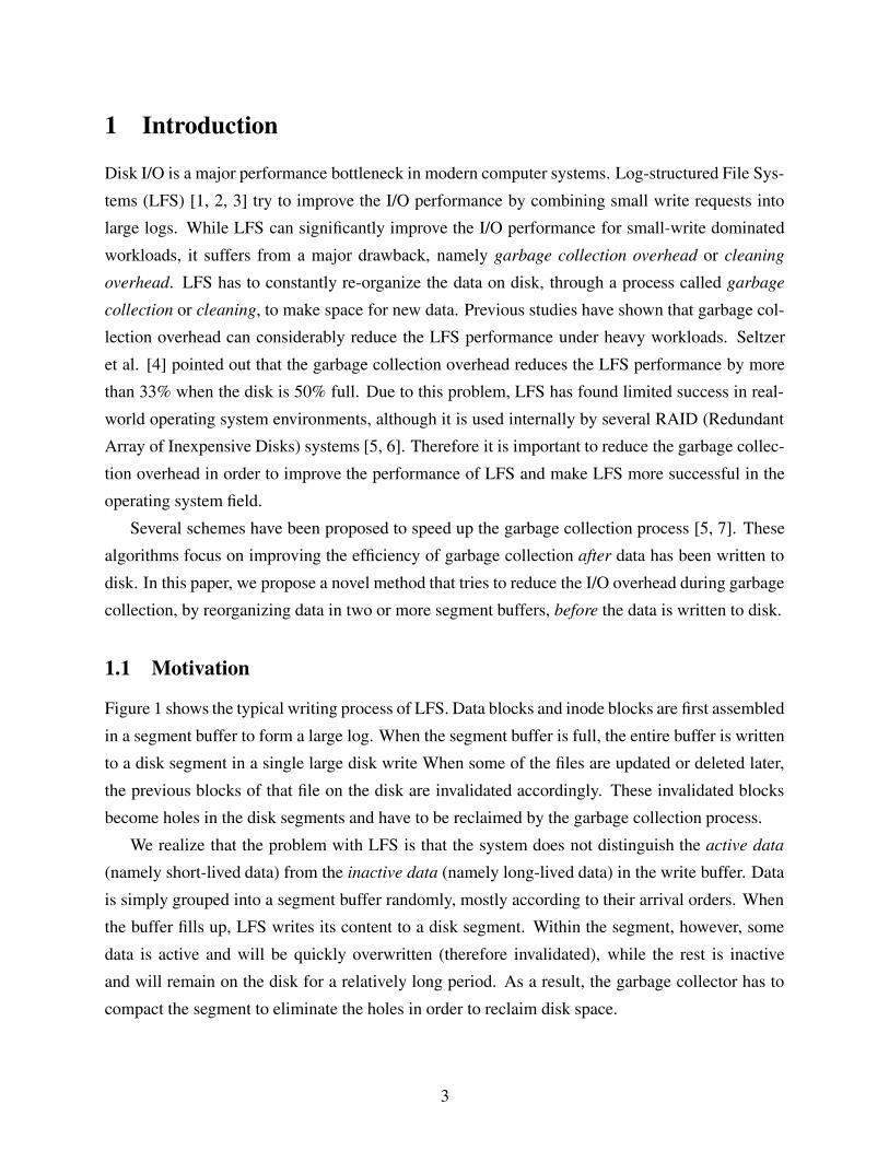
Figure 1 shows the typical writing process of LFS. Data blocks and inode blocks are first assembled

in a segment buffer to form a large log. When the segment buffer is full, the entire buffer is written

to a disk segment in a single large disk write When some of the files are updated or deleted later,

the previous blocks of that file on the disk are invalidated accordingly. These invalidated blocks

become holes in the disk segments and have to be reclaimed by the garbage collection process.

We realize that the problem with LFS is that the system does not distinguish the active data

(namely short-lived data) from the inactive data (namely long-lived data) in the write buffer. Data

is simply grouped into a segment buffer randomly, mostly according to their arrival orders. When

the buffer fills up, LFS writes its content to a disk segment. Within the segment, however, some

data is active and will be quickly overwritten (therefore invalidated), while the rest is inactive

and will remain on the disk for a relatively long period. As a result, the garbage collector has to

compact the segment to eliminate the holes in order to reclaim disk space.

3

��

��

��

��

��

��

��

��

��

��

��

��

��

��

��

��

��

��

��

��

��

��

��

��

��

��

��

��

��

��Disk

Disk

(1) Data blocks first enter a Segment BufferBuffer

(3) After a while, many blocks in segments are invalidated, leaving holes and require garbage collection

......

......

Data

(2) Buffer written to disk when full (Shown two newly written segments here)

��

��

��

��

��

��

��

��

��

��

��

��

��

��

��

��

��

��

��

��

��

��

��

��

Valid data block Invalidated block (hole)Empty block

Figure 1: The writing process of LFS

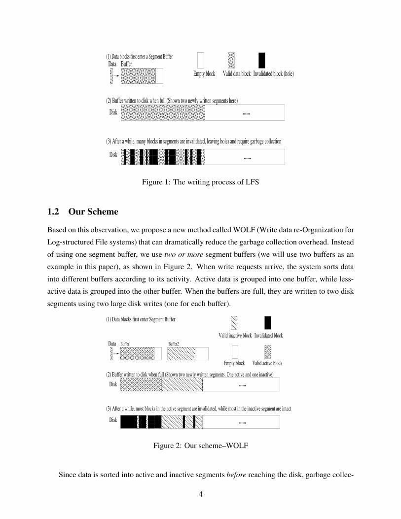
1.2 Our Scheme

Based on this observation, we propose a new method called WOLF (Write data re-Organization for

Log-structured File systems) that can dramatically reduce the garbage collection overhead. Instead

of using one segment buffer, we use two or more segment buffers (we will use two buffers as an

example in this paper), as shown in Figure 2. When write requests arrive, the system sorts data

into different buffers according to its activity. Active data is grouped into one buffer, while less-

active data is grouped into the other buffer. When the buffers are full, they are written to two disk

segments using two large disk writes (one for each buffer).

��

��

Buffer2

��

��

��

��

��

��

��

��

��

��

��

��

��

��

��

��

��

��

��

��

��

��

(1) Data blocks first enter Segment Buffer

Data

Disk

Disk

......

(2) Buffer written to disk when full (Shown two newly written segments. One active and one inactive)

......

(3) After a while, most blocks in the active segment are invalidated, while most in the inactive segment are intact

Buffer1

Valid inactive block

��

��

��

��

Empty block Valid active block

Invalidated block

Figure 2: Our scheme–WOLF

Since data is sorted into active and inactive segments before reaching the disk, garbage collec-

4

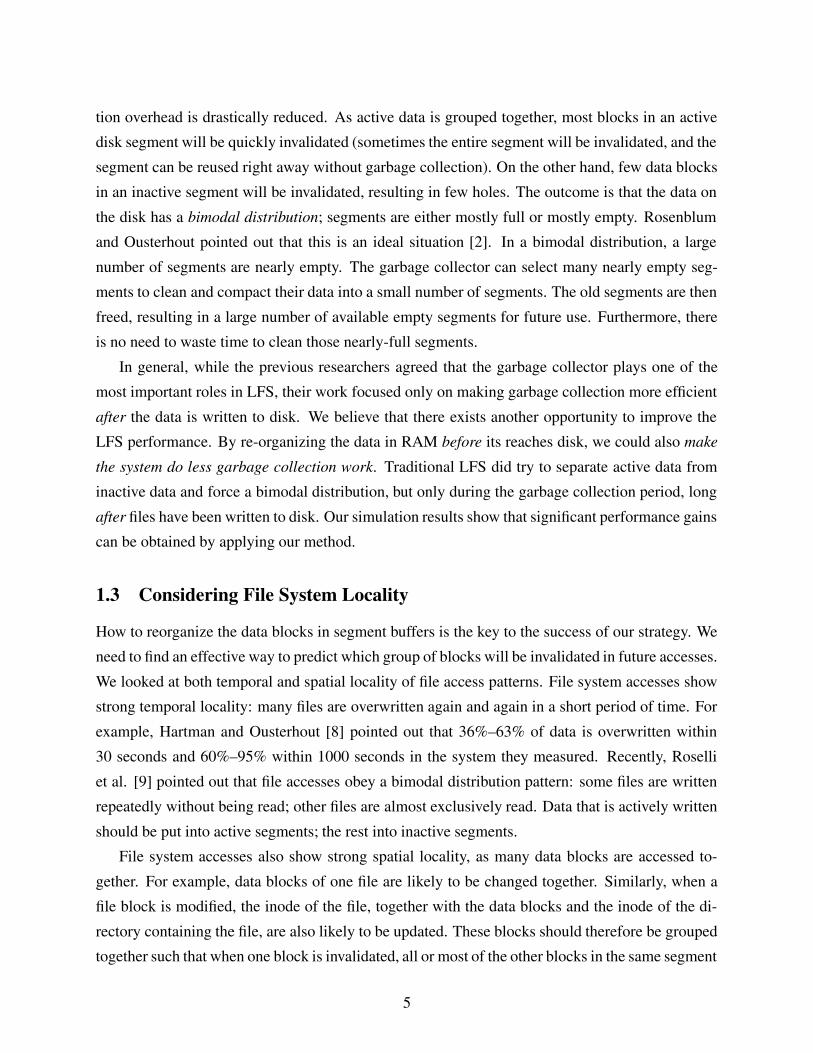
tion overhead is drastically reduced. As active data is grouped together, most blocks in an active

disk segment will be quickly invalidated (sometimes the entire segment will be invalidated, and the

segment can be reused right away without garbage collection). On the other hand, few data blocks

in an inactive segment will be invalidated, resulting in few holes. The outcome is that the data on

the disk has a bimodal distribution; segments are either mostly full or mostly empty. Rosenblum

and Ousterhout pointed out that this is an ideal situation [2]. In a bimodal distribution, a large

number of segments are nearly empty. The garbage collector can select many nearly empty seg-

ments to clean and compact their data into a small number of segments. The old segments are then

freed, resulting in a large number of available empty segments for future use. Furthermore, there

is no need to waste time to clean those nearly-full segments.

In general, while the previous researchers agreed that the garbage collector plays one of the

most important roles in LFS, their work focused only on making garbage collection more efficient

after the data is written to disk. We believe that there exists another opportunity to improve the

LFS performance. By re-organizing the data in RAM before its reaches disk, we could also make

the system do less garbage collection work. Traditional LFS did try to separate active data from

inactive data and force a bimodal distribution, but only during the garbage collection period, long

after files have been written to disk. Our simulation results show that significant performance gains

can be obtained by applying our method.

1.3 Considering File System Locality

How to reorganize the data blocks in segment buffers is the key to the success of our strategy. We

need to find an effective way to predict which group of blocks will be invalidated in future accesses.

We looked at both temporal and spatial locality of file access patterns. File system accesses show

strong temporal locality: many files are overwritten again and again in a short period of time. For

example, Hartman and Ousterhout [8] pointed out that 36%–63% of data is overwritten within

30 seconds and 60%–95% within 1000 seconds in the system they measured. Recently, Roselli

et al. [9] pointed out that file accesses obey a bimodal distribution pattern: some files are written

repeatedly without being read; other files are almost exclusively read. Data that is actively written

should be put into active segments; the rest into inactive segments.

File system accesses also show strong spatial locality, as many data blocks are accessed to-

gether. For example, data blocks of one file are likely to be changed together. Similarly, when a

file block is modified, the inode of the file, together with the data blocks and the inode of the di-

rectory containing the file, are also likely to be updated. These blocks should therefore be grouped

together such that when one block is invalidated, all or most of the other blocks in the same segment

5

will also be invalidated.

1.4 Organization of This Paper

The remainder of the paper is organized as follows. Section 2 discusses related work. Section

3 describes our design of WOLF. Section 4 describes our experimental methodology. Section 5

presents the simulation results and analysis. Section 6 summarizes our new strategy.

2 Related Work

Ousterhout et al. proposed Log-structured File Systems (LFS) to manage disk storage [1, 2]. LFS

writes all updates to disk sequentially in a log-like structure, thereby improving both the file write

performance and crash recovery. Seltzer et al. [3, 4] developed an implementation of LFS for BSD

Unix. They used an index file to maintain the memory-consuming data structures like the inode

map.

Several new garbage collection policies have been presented [5, 7, 10] to overcome the high

garbage collection overhead of LFS. In traditional garbage collection policies [2], including greedy

cleaning and cost-age cleaning, live blocks in several partially empty segments are combined to

produce a new full segment, freeing the old partially empty segments for reuse. These policies

perform well when the disk space utilization is low. Wilkes et al. [5] proposed the hole-plugging

policy. In their scheme, partially empty segments are freed by writing their live blocks into the

holes found in other segments. Despite the higher per-block cost, at high disk utilization, hole-

plugging performs better than traditional garbage collection because it avoids processing too many

segments. Recently, Matthews et al. [7] showed how adaptive algorithms can be used to enable

LFS to provide high performance across a wider range of workloads. Their algorithms automat-

ically select either the benefit-to-cost or the hole-plugging method depending on cost-benefit es-

timates. They also used cached data to lower garbage collection costs. Blackwell et al. [10]

presented a heuristic algorithm that does not interfere with normal file accesses. They found that

97% of garbage collection on the most heavily loaded system was done in the background. Re-

cently, we proposed a scheme [11] that incorporates the knowledge of Zone-Bit-Recording into

LFS to improve both the read and write performance. It reorganizes data on the disk during the

LFS garbage collection and the system idle periods. By putting active data in the faster zones and

inactive data in the slower zones, we can achieve performance improvements for both reads and

writes.

6

The strategy proposed in this paper is distinctively different from the above methods : WOLF

works with the initial write data in the reordering write buffers, reducing the garbage collection

overhead before the data goes to the disk. As a result, WOLF can be easily combined with other

strategies to further improve the LFS performance.

3 The Design of WOLF

The main operations of WOLF include writing, reading, garbage collection and crash-recovery.

Another important action is the separation of active-data from inactive data, which is invoked by

each write operation.

3.1 Writing

After the system receives a write request, WOLF decides if the requested data is active or inactive

and puts the data into one of the segment buffers accordingly. (We will discuss how to do this in

Section 3.3.) The corresponding old data in a disk segment is also invalidated. The request is then

considered complete.

When the write buffers are full, all buffers are written to some free disk segments in large write

requests in order to amortize the cost of many small writes. Since WOLF contains several segment

buffers and each buffer is written into a different disk segment, several large writes occur during

the process (one large write for each buffer).

As in LFS, WOLF also writes buffers to the disk when one of the following conditions is

satisfied, even when the buffers are not full:

• A buffer contains data modified more than 30 seconds ago.

• An fsync or sync occurs

Since LFS uses a single segment buffer, only one large write is issued when a buffer write is

invoked. On the contrary, WOLF maintains two or more segment buffers. To simplify the crash

recovery process (to be discussed in Section 3.4), when WOLF has to write the data to disk, all

segment buffers in RAM will be written (logged) to the disk at the same time. While the logging

process contains several large disk write operations, WOLF considers the log operation atomic. A

logging is considered successful only if all segment buffers are successfully written to the disk.

The atomic logging feature means that we can view the multiple physical segments of WOLF as a

single virtual segment.

7

The atomic writing of multiple segments can easily be achieved with a time stamp. All seg-

ments written together will have the same time stamp and the same “# of segments written to-

gether” field. During crash recovery, the system searches for the segments with the latest time

stamp. If the number of segments with the same latest time stamp matches the “# of segments

written together” field, then the system knows that the last log-writing operation was successful.

3.2 Reading

WOLF only changes the write cache structures of LFS. The read operations are not affected. Our

experiments show that WOLF and LFS have similar read performances.

3.3 Separating Active and Inactive data

The key to the design of WOLF is an efficient and easy-to-implement algorithm to separate active

data from inactive data and puts them into different buffers accordingly.

3.3.1 An Adaptive Grouping Algorithm

We developed a heuristic learning method for WOLF, which is a variation of the least-recently

used algorithm with frequency information.

Figure 3 describes our algorithm in detail. The idea is similar to virtual memory page-aging

techniques. The system maintains a reordering buffer that tracks recently accessed data blocks.

Each entry in the buffer contains a reference count and other address information (e.g., a pointer

to the corresponding buffer cache block). To capture the temporal locality of file accesses, the

reference count is incremented when the block is accessed. The count is initialized to zero and is

also reset to zero when the file system becomes idle for a certain period. We call this period as a

time-bar, which it is initialized to 10 minutes. If the age of a block exceeds the current time-bar,

WOLF will reset its reference count to zero. The value of the count indicates the activity level of

the block in the most recent active period: The higher the value of the count, the more active the

block is. The time-bar could be adaptively tuned for various incoming accesses. When the system

identifies that there is no significant difference among the blocks’ activity ratios in the reorder

buffers, for example, 90% of the blocks have the same reference counts, the value of the time-bar

is doubled. If most blocks have different activity ratios, for example, only 10% of the blocks have

the same reference counts, the time-bar is halved. The time-bar makes the reordering buffers work

heuristically for different workloads. Active data is then put into the active segment buffer, and

other data in the inactive buffer.

8

Algorithm Aim to reorder data blocks in the reordering write buffer and produce segment buffers with different activity behavior

ReorderingWriteBuffer() Begin

Sort all blocks in the reordering write buffer based on their activity ratios in an ascending order. /*Next, we group these blocks into two or more separate segment buffers with different active behavior*/ While NOT (Finish filling segment buffers or blocks)

Fill blocks from the least active side into a segment buffer until the buffer is full. EndWhile /*Check whether current activity ratios accurately reflect blocks’ activities or not; if not, modify timebar*/ If (90% of activity ratios are equal) Then timebar = timebar × 2; Else If (10% of activity ratios are equal)

Then timebar = timebar / 2; /*Reset blocks’ activity ratios after a period*/ While NOT (Finish scanning all blocks in the reordering buffer)

If (A block’s age is older than timebar) Then Reset its activity ratio to zero.

EndWhile End /*ReorderingWriteBuffer()*/

Figure 3: Adaptive Grouping Algorithm

If two blocks have the same reference count value, then spatial locality is considered. If the

two blocks satisfy one of the following conditions, they will be grouped into the same segment

buffer:

• The two blocks belong to the same file.

• The two blocks belong to files in the same directory.

If neither of the above conditions is true, the blocks are randomly assigned buffers.

The overhead of this learning method is low. Most blocks receive no more than a hundred

accesses in a time-bar period. Only a few additional bits are added for each block. The time-bar is

managed by the reordering buffer manager with little overhead.

9

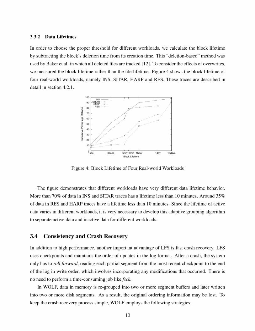
3.3.2 Data Lifetimes

In order to choose the proper threshold for different workloads, we calculate the block lifetime

by subtracting the block’s deletion time from its creation time. This “deletion-based” method was

used by Baker et al. in which all deleted files are tracked [12]. To consider the effects of overwrites,

we measured the block lifetime rather than the file lifetime. Figure 4 shows the block lifetime of

four real-world workloads, namely INS, SITAR, HARP and RES. These traces are described in

detail in section 4.2.1.

0

10

20

30

40

50

60

70

80

90

100

1sec 30sec 5min 10min 1hour 1day 10days

Cum

ulat

ive

Per

cent

age

of B

lock

s

Block Lifetime

INSSITARHARP

RES

Figure 4: Block Lifetime of Four Real-world Workloads

The figure demonstrates that different workloads have very different data lifetime behavior.

More than 70% of data in INS and SITAR traces has a lifetime less than 10 minutes. Around 35%

of data in RES and HARP traces have a lifetime less than 10 minutes. Since the lifetime of active

data varies in different workloads, it is very necessary to develop this adaptive grouping algorithm

to separate active data and inactive data for different workloads.

3.4 Consistency and Crash Recovery

In addition to high performance, another important advantage of LFS is fast crash recovery. LFS

uses checkpoints and maintains the order of updates in the log format. After a crash, the system

only has to roll forward, reading each partial segment from the most recent checkpoint to the end

of the log in write order, which involves incorporating any modifications that occurred. There is

no need to perform a time-consuming job like fsck.

In WOLF, data in memory is re-grouped into two or more segment buffers and later written

into two or more disk segments. As a result, the original ordering information may be lost. To

keep the crash recovery process simple, WOLF employs the following strategies:

10

1. While data blocks are reordered by WOLF to improve the performance, their original arrival

ordering information is kept in a data structure and written to disk in the summary block

together with each segment.

2. While WOLF maintains two or more segment buffers, its atomic logging feature (discussed

in Section 3.1) means that these multiple physical buffers can be viewed as a single virtual

segment.

Since WOLF maintains only a single virtual segment which is logged atomically, and the in-

formation about original arrival orders of data blocks in the virtual segment is preserved, WOLF

enjoys the same simple crash recovery advantage as LFS.

3.5 Garbage Collection

3.5.1 The Garbage Collector

Previous research shows that a single garbage collection algorithm is unlikely to perform equally

well for all kinds of workloads. The benefit-to-cost algorithm works well in most cases while the

hole-plugging policy works well when the disk segment utilization is very high. As a result, we

chose the same adaptive method used by Matthews et al. [7]. This policy automatically selects

either the benefit-to-cost or the hole-plugging method depending on cost-benefit estimates.

In WOLF, the garbage collector runs when the system is idle or the disk utilization exceeds

a high water-mark. In our simulation, the high water-mark is 80% of the disk capacity. Idle

is defined as the file system been inactive for 5 minutes. The amount of data that the garbage

collection may process at one time can be varied. In this paper, we allowed the garbage collection

to process up to 20 MB at one time.

3.5.2 Garbage Collection Overheads

To calculate the benefit and overhead of garbage collection, we used the following mathematical

model. These formulae were developed by Rosenblum et al. [2] and Matthews et al. [7]. For a

complete and detailed analysis, please refer to the original papers [2, 7].

In the following discussion, cost implies the total time to perform the garbage collection, while

benefit represents free space being reclaimed.

The benefit-to-cost ratio is defined as follows:

benefit

cost=

(1 − utilization) ∗ age of segment

(1 + utilization)

11

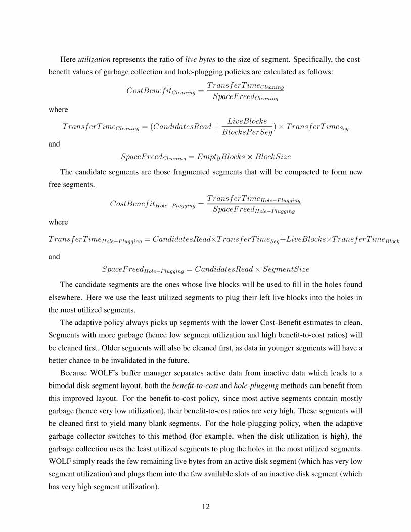
Here utilization represents the ratio of live bytes to the size of segment. Specifically, the cost-

benefit values of garbage collection and hole-plugging policies are calculated as follows:

CostBenefitCleaning =TransferT imeCleaning

SpaceFreedCleaning

where

TransferT imeCleaning = (CandidatesRead +LiveBlocks

BlocksPerSeg) × TransferT imeSeg

and

SpaceFreedCleaning = EmptyBlocks × BlockSize

The candidate segments are those fragmented segments that will be compacted to form new

free segments.

CostBenefitHole−P lugging =TransferT imeHole−P lugging

SpaceFreedHole−P lugging

where

TransferT imeHole−P lugging = CandidatesRead×TransferT imeSeg+LiveBlocks×TransferT imeBlock

and

SpaceFreedHole−P lugging = CandidatesRead × SegmentSize

The candidate segments are the ones whose live blocks will be used to fill in the holes found

elsewhere. Here we use the least utilized segments to plug their left live blocks into the holes in

the most utilized segments.

The adaptive policy always picks up segments with the lower Cost-Benefit estimates to clean.

Segments with more garbage (hence low segment utilization and high benefit-to-cost ratios) will

be cleaned first. Older segments will also be cleaned first, as data in younger segments will have a

better chance to be invalidated in the future.

Because WOLF’s buffer manager separates active data from inactive data which leads to a

bimodal disk segment layout, both the benefit-to-cost and hole-plugging methods can benefit from

this improved layout. For the benefit-to-cost policy, since most active segments contain mostly

garbage (hence very low utilization), their benefit-to-cost ratios are very high. These segments will

be cleaned first to yield many blank segments. For the hole-plugging policy, when the adaptive

garbage collector switches to this method (for example, when the disk utilization is high), the

garbage collection uses the least utilized segments to plug the holes in the most utilized segments.

WOLF simply reads the few remaining live bytes from an active disk segment (which has very low

segment utilization) and plugs them into the few available slots of an inactive disk segment (which

has very high segment utilization).

12

4 Experimental Methodology

We used trace-driven simulation experiments to evaluate the effectiveness of our proposed new

design. Both real-world and synthetic traces were used during simulation. In order to make our

experiments and simulation results more convincing, we used four different real-world traces and

four synthetic traces to cover a wide variety of workloads.

4.1 The Simulators

The WOLF simulator contains more than 8,000 lines of C++ code. It consists of an LFS simulator,

which acts as a file system, on top of a disk simulator. The disk model is based on Ganger’s

DiskSim [13]. Our LFS simulator is developed based on Sprite LFS. We ported the LFS code from

the Sprite LFS kernel distribution and implemented a trace-driven class to accept trace files. By

changing a configuration file, we can vary important parameters such as the number of segment

buffers, the segment size and the read cache size. In the simulator, data is channeled into the log

through several write buffers. The write buffers are flushed every 30 seconds of simulated time to

capture the impact of partial segment writes. A segment usage table is implemented to maintain

the status of disk segments. Meta-data structures including the summary block and inode map are

also developed. We built a checkpoint data structure to periodically save blocks of the inode map

and the segment usage table.

The disk performance characteristics are set in DiskSim’s configuration files. We chose two

disk models during simulation, a small (1 GB capacity) HP2247A disk and a large (9.1 GB) Quan-

tum Atlas10K disk. The small HP2247A was used for SITAR and HARP traces, because the two

traces have small data-sets (total data accessed < 1 GB). A small disk is needed in order to ob-

serve the garbage collection activities. The large disk was used for all other traces. Using two

significantly different disks also helps us to investigate the impacts of disk features like capacity

and speed on WOLF performance. The HP2247A’s spindle speed is 5400 RPM. The read-channel

bandwidth is 5 MB/sec. Its average access time is 15 ms. The Quantum Atlas10K has a 10024

RPM spindle speed. Its read-channel bandwidth is 60 MB/sec and average access time 6 ms.

4.2 Workload Models

The purpose of our experiments is to conduct a comprehensive and unbiased performance study

of the proposed scheme and compare the results with that of LFS. We paid special attention to

selecting the traces. Our main objective was to select traces that match realistic workloads as

13

closely as possible. At the same time, we also wanted to cover as wide a range of environments as

possible. Several sets of trace files have been selected in this paper as discussed below.

4.2.1 Real-world Traces

Four real-world file system traces were used in our simulation. We obtained two sets of real-life

traces from two different universities to validate our results. Two of them, from University of Cal-

ifornia at Berkeley, are called INS and RES [9]. INS was collected from a group of 20 machines

located in labs for undergraduate classes. RES was collected on a system consisting of 13 desktop

machines of a research group. INS and RES were based on 112 days of traces from September

1996 to December 1996. The other set of two traces from University of Kentucky contain all

disk activities on two SunOS 4.1 machines during ten days for SITAR and seven days for HARP

[14]. SITAR represents an office environment while HARP reflects common program develop-

ment activities. More specifically, SITAR is a collection of file accesses by graduate students and

professors doing work such as sending and receiving email, compiling programs, running LaTeX,

editing files, and so on. HARP trace represents a collaboration of two graduate students working

on a single multimedia application. Because SITAR and HARP have small working sets, we used

the small disk model for these two real-world traces. Notice in the experiments, we expanded

SITAR and HARP by appending files with same access pattern as in the original traces but with

different file names, in order to explore the system behavior under varying disk utilization. For

large traces with more than 10 GB data traffic, we did not perform such expansions.

4.2.2 Synthetic Traces

While real-world traces give a realistic representation of some actual systems, synthetic traces have

the advantage of being flexible. We therefore also generated a set of synthetic traces. We varied the

trace characteristics as much as possible in order to cover a very wide range of different workloads.

We generated the following four sets of synthetic traces:

1. Uniform Pattern (Uniform)

Each file has equal likelihood of being selected.

2. Hot-and-cold Pattern (Hot-cold)

Files are divided into two groups. One group contains 10% of files; it is called hot group

because its files are visited 90% of the time. The other group is called cold; it contains 90%

of the files but they are visited only 10% of the time. Within each groups, files are equally

likely to be visited. This access pattern models a simple form of locality.

14

3. Ephemeral Small File Regime (Small Files)

This suite contains small files and tries to model the behavior of systems such as the elec-

tronic mail or network news systems. The sizes of files are limited from 1 KB to 1 MB. They

are frequently created, deleted and updated. The data lifetime of this suite is the shortest one

among all traces used in this paper: 90% of block lifetimes are less than 5 minutes.

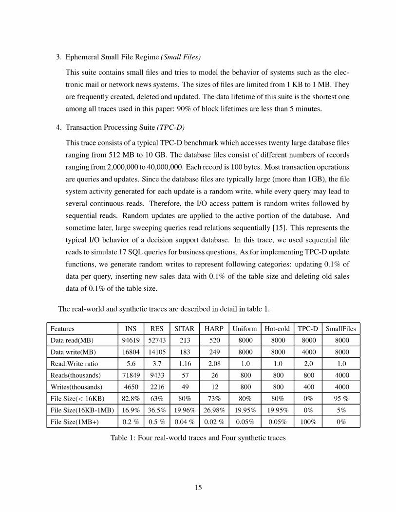
4. Transaction Processing Suite (TPC-D)

This trace consists of a typical TPC-D benchmark which accesses twenty large database files

ranging from 512 MB to 10 GB. The database files consist of different numbers of records

ranging from 2,000,000 to 40,000,000. Each record is 100 bytes. Most transaction operations

are queries and updates. Since the database files are typically large (more than 1GB), the file

system activity generated for each update is a random write, while every query may lead to

several continuous reads. Therefore, the I/O access pattern is random writes followed by

sequential reads. Random updates are applied to the active portion of the database. And

sometime later, large sweeping queries read relations sequentially [15]. This represents the

typical I/O behavior of a decision support database. In this trace, we used sequential file

reads to simulate 17 SQL queries for business questions. As for implementing TPC-D update

functions, we generate random writes to represent following categories: updating 0.1% of

data per query, inserting new sales data with 0.1% of the table size and deleting old sales

data of 0.1% of the table size.

The real-world and synthetic traces are described in detail in table 1.

Features INS RES SITAR HARP Uniform Hot-cold TPC-D SmallFiles

Data read(MB) 94619 52743 213 520 8000 8000 8000 8000

Data write(MB) 16804 14105 183 249 8000 8000 4000 8000

Read:Write ratio 5.6 3.7 1.16 2.08 1.0 1.0 2.0 1.0

Reads(thousands) 71849 9433 57 26 800 800 800 4000

Writes(thousands) 4650 2216 49 12 800 800 400 4000

File Size(< 16KB) 82.8% 63% 80% 73% 80% 80% 0% 95 %

File Size(16KB-1MB) 16.9% 36.5% 19.96% 26.98% 19.95% 19.95% 0% 5%

File Size(1MB+) 0.2 % 0.5 % 0.04 % 0.02 % 0.05% 0.05% 100% 0%

Table 1: Four real-world traces and Four synthetic traces

15

5 Simulation Results and Performance Analysis

In order to understand the behavior of WOLF, we compare our design with the most recent LFS

version using the adaptive garbage collection method, which acts as the baseline system. WOLF

also uses the same adaptive garbage collection method. As a result, we can study the impact of our

reordering write buffers rather than that of the garbage collection policy.

In the experiments, the following default parameters are used unless otherwise specified: the

buffer cache size is 64 MB, each disk segment is 256 KB and each segment buffer is 256 KB.

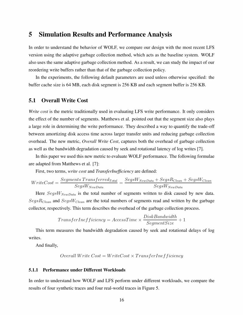
5.1 Overall Write Cost

Write cost is the metric traditionally used in evaluating LFS write performance. It only considers

the effect of the number of segments. Matthews et al. pointed out that the segment size also plays

a large role in determining the write performance. They described a way to quantify the trade-off

between amortizing disk access time across larger transfer units and reducing garbage collection

overhead. The new metric, Overall Write Cost, captures both the overhead of garbage collection

as well as the bandwidth degradation caused by seek and rotational latency of log writes [7].

In this paper we used this new metric to evaluate WOLF performance. The following formulae

are adapted from Matthews et al. [7]:

First, two terms, write cost and TransferInefficiency are defined:

WriteCost =Segments TransferredTotal

SegsWNewData

=SegsWNewData + SegsRClean + SegsWClean

SegsWNewData

Here SegsWNewData is the total number of segments written to disk caused by new data.

SegsRClean and SegsWClean are the total numbers of segments read and written by the garbage

collector, respectively. This term describes the overhead of the garbage collection process.

TransferInefficiency = AccessT ime × DiskBandwidth

SegmentSize+ 1

This term measures the bandwidth degradation caused by seek and rotational delays of log

writes.

And finally,

Overall Write Cost = WriteCost × TransferInefficiency

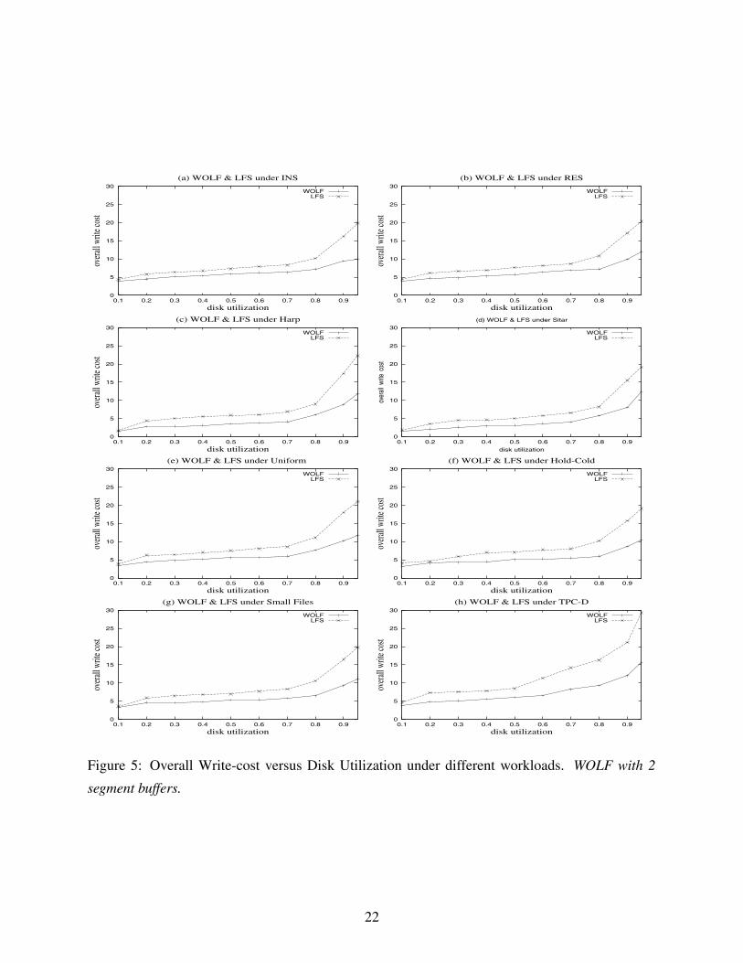
5.1.1 Performance under Different Workloads

In order to understand how WOLF and LFS perform under different workloads, we compare the

results of four synthetic traces and four real-world traces in Figure 5.

16

It is clear from the figure that WOLF significantly reduces the overall write cost compared to

LFS. The new design reduces the overall write cost by up to 53%. The overall write cost is further

reduced when the disk space utilization is higher.

Although the eight traces have very different characteristics, we can see that the performance of

WOLF is not sensitive to variations in these workloads. This is because the heuristic reorganizing

algorithm is adaptive to the changing behavior in file accesses. On the other hand, LFS performs

especially poor for the TPC-D workload (it has the highest overall write-cost among all workloads)

because of its random updating behavior, especially under high disk utilization. This is not a

surprise. Similar behavior was observed by Seltzer and Smith in [4]. WOLF, on the other hand,

significantly reduces garbage collection overhead so it performs well under TPC-D.

5.1.2 Effects of Number of Segment Buffers

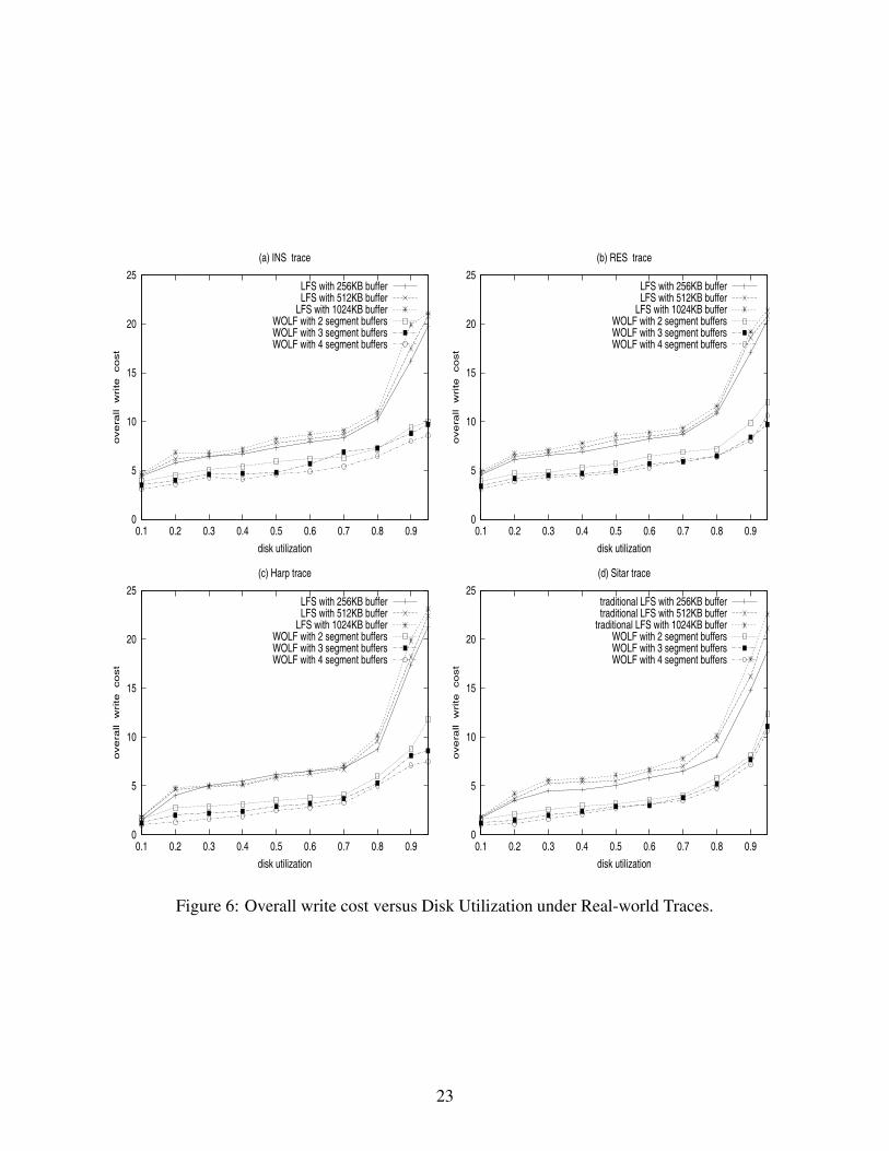
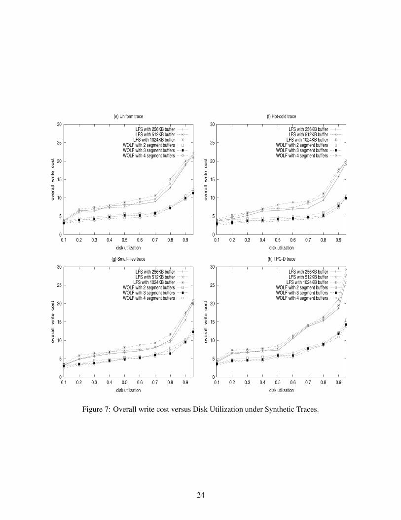
Figures 6 and 7 show the results of the overall write cost versus disk utilization for the four real-

world traces and four synthetic traces, respectively. We varied the number of segment buffers of

WOLF from 2 to 4. We also varied the segment buffer size of LFS from 256 KB to 1024 KB.

Increasing the number of segment buffers in WOLF slightly reduces the overall write cost but

does not have a significant impact on the overall performance.

The reason we studied LFS with different segment buffer sizes is to show that the performance

gain of WOLF is not due to the increased buffer numbers (hence the increased total buffer size).

The separated active/inactive data layout on the disk segments contributes to the performance im-

provement. In fact, for LFS, increasing the segment buffer sizes may actually increase the overall

write cost. This observation is consistent with previous studies [2, 7].

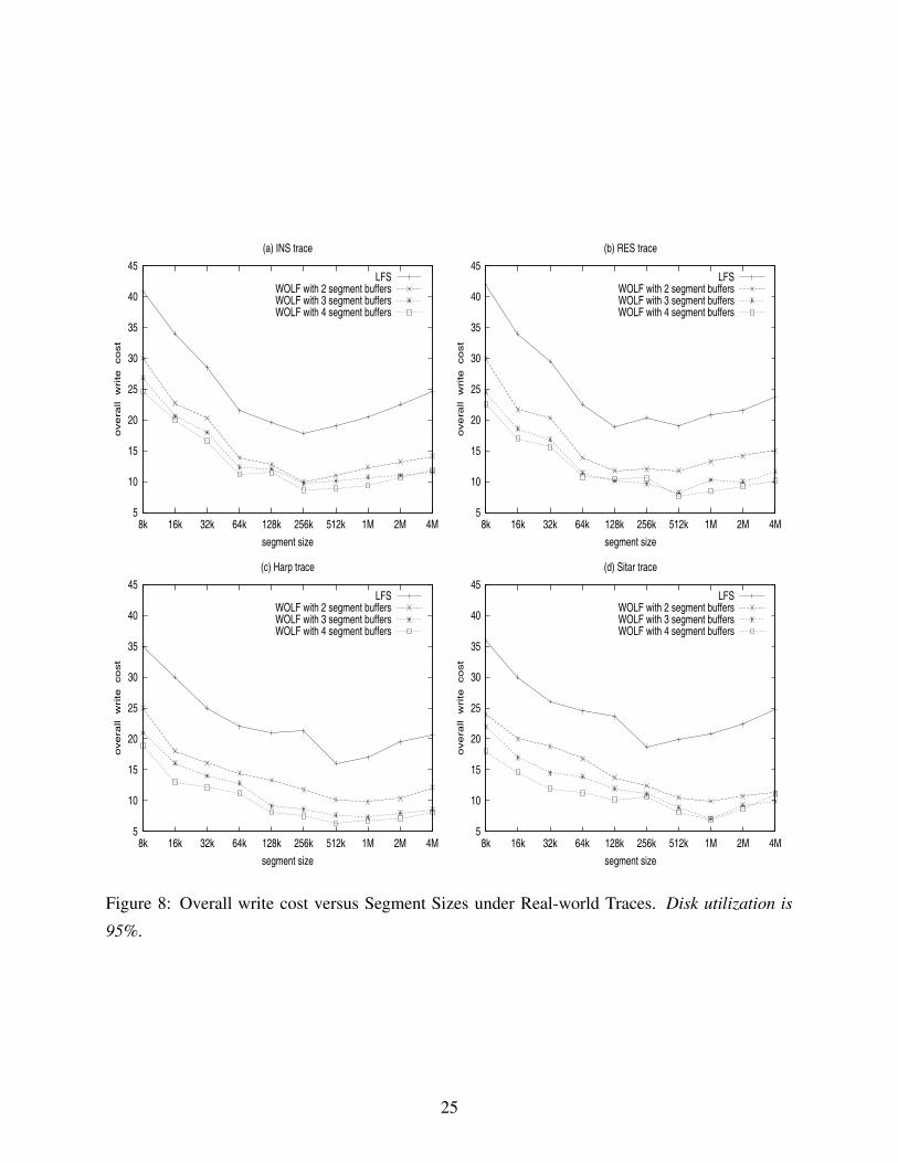
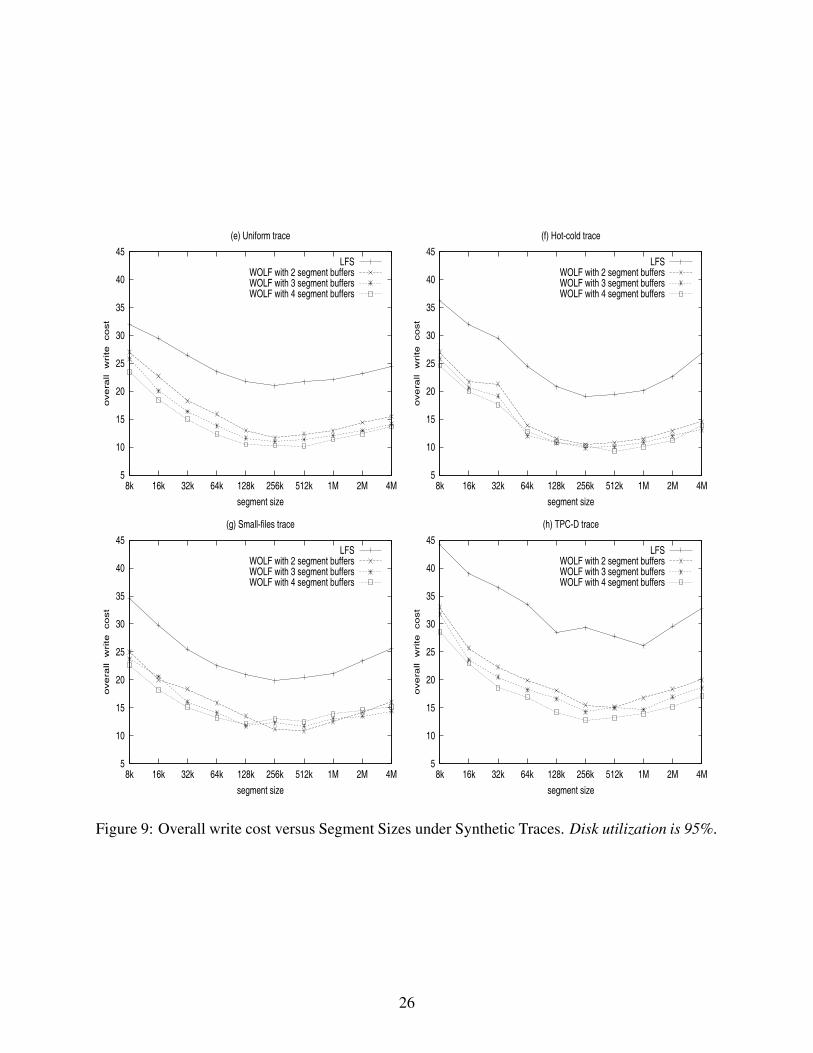
5.1.3 Effects of Segment Sizes

The size of the disk segment is also an important factor for the performance of both WOLF and

LFS. If the size is too large, it would be difficult to find enough active data to fill one segment and

enough inactive data for another segment. The result will be that the active data and the inactive

data are mixed together in a large segment, resulting in poor garbage collection performance. The

limited disk bandwidth will also have a negative impact on the overall write cost when the segment

buffer size exceeds a threshold. On the contrary, if the segment size is too small, the original

benefit of LFS, namely taking advantage of large disk transfers, is lost.

Figures 8 and 9 show the overall write cost versus the sizes of segment buffers under real-world

traces and synthetic traces, respectively. We can see that for both WOLF and LFS, a segment size

between 256-1024 KB is good for all these workloads.

17

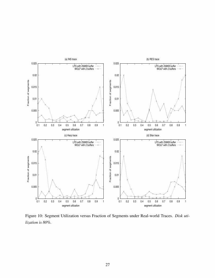
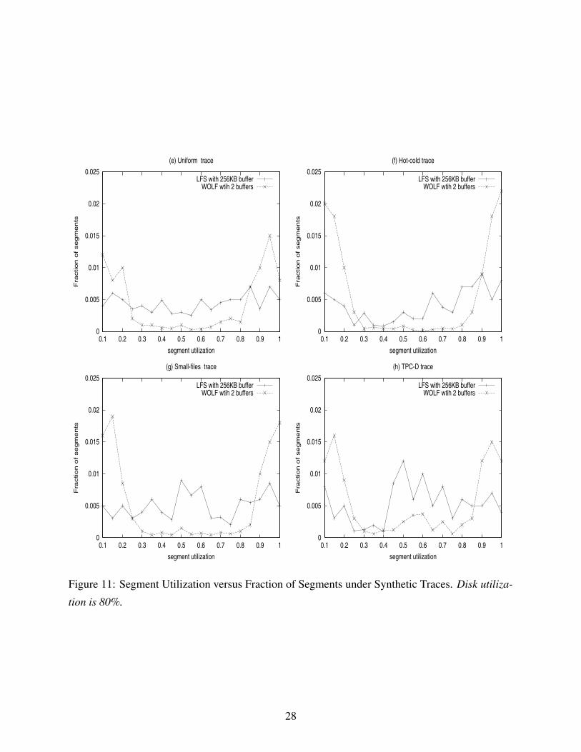
5.1.4 Segment Utilization Distribution

In order to gain insight into why WOLF significantly outperforms LFS, we also compared the

segment utilization distributions of WOLF and LFS. Segment utilization is calculated by the total

live bytes in the segment divided by the size of the segment.

Figures 10 and 11 show the distribution of segment utilization under the four real-world traces

and four synthetic traces, respectively. We can see the obvious bimodal segment distribution in

WOLF when compared to LFS. Such a bimodal distribution is the key to the performance ad-

vantage of WOLF over LFS. Harp and Hot-cold traces have better results because our heuristic

grouping algorithm works better under such workloads with distinctively repeated accesses. The

TPC-D trace has the worst distribution because it has many random updates.

5.2 File System Performance

In the previous discussion, we used overall write cost as the performance metric. Overall write

cost is a direct measurement of system efficiency. We have shown that WOLF performs noticeably

better than LFS, as the former has a much smaller overall write cost.

However, end-users would be more interested in user-measurable metrics such as the access

latency [16]. The overall write cost quantifies the additional I/O overhead when LFS performs

garbage collection. LFS performance is sensitive to this overhead. To see whether the lower

overall write cost in WOLF will result in lower access latencies, we also measured the average file

read/write response times at the file system level. All these results include the garbage collection

overhead.

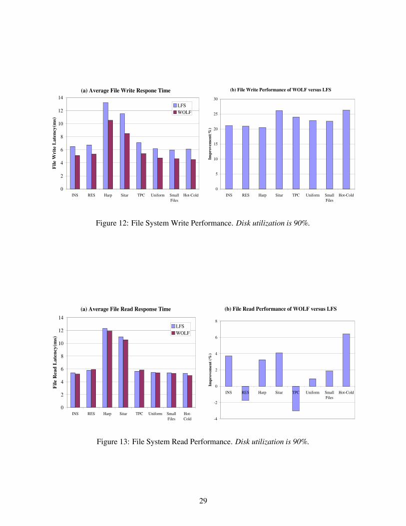
5.2.1 Write Response Times

Figure 12(a) shows file write response times of LFS and WOLF under eight traces. Figure 12(b)

plots the performance improvement of WOLF over LFS. We can see that WOLF improves write

response times by 20–26%. The lower overall write cost in WOLF directly leads to a smaller write

response time. The Hot-cold trace achieves the best improvement because of its good locality.

5.2.2 Read Response Times

Figure 13(a) shows the file read performance of LFS and WOLF under eight traces. Figure 13(b)

plots the performance improvement of WOLF over LFS. The results show that, for most traces, the

read performance of WOLF is comparable to that of LFS. The small differences between the two

systems are mostly within the experimental error range.

18

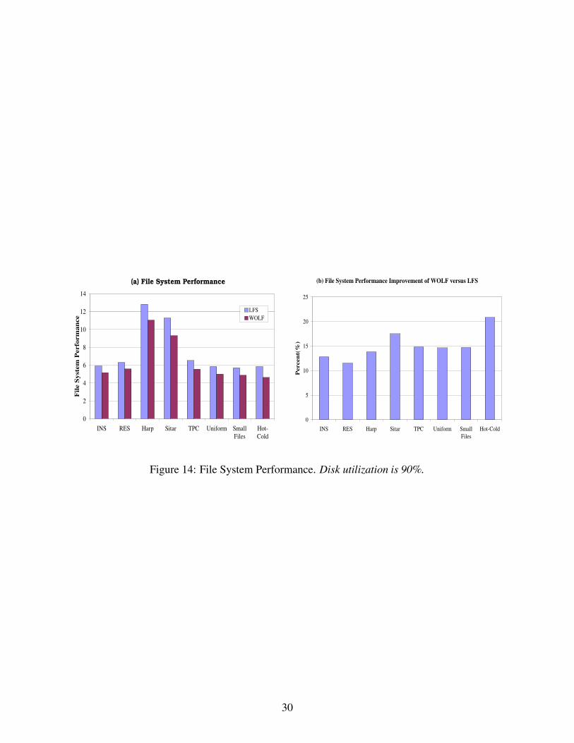
5.2.3 Overall File System Response Times

Figure 14(a) shows overall file system response times (including both reads and writes) of LFS and

WOLF under eight traces. Figure 14(b) plots the performance improvement of WOLF over LFS.

For all traces, WOLF outperforms LFS from 12% to 21%.

5.3 Implication of Different Disk Models

Our numbers show that WOLF achieves significant performance gains for both the small/slow and

the large/fast disk models. The results suggest that the disk characteristics do not have a direct

impact on WOLF. While the absolute performance parameters may vary on different disk models,

the overall trend is clear: WOLF can markedly reduce garbage collection overhead under many

different workloads on different disk models.

6 Conclusion and Future Work

We have presented a novel reordering write buffer design called WOLF for Log-structured File

Systems. WOLF improves the disk layout by reordering write data in segment buffers before

writing the data to disk. By utilizing an adaptively heuristic grouping algorithm that separates

active data from inactive data, and taking advantage of file temporal and spatial localities, the

reordering buffer forces the actively-accessed data blocks into one (hot) segment and the inactive

data into another (cold) segment. Most of the blocks in active segments will be quickly invalidated,

while most blocks in inactive segments will be left intact. Data on disk therefore forms a bimodal

distribution, which significantly reduces garbage collection overhead.

Since WOLF works before the initial write data reaches the disk, it can be integrated with

other existing strategies smoothly to improve LFS performance. By reducing garbage collection

overhead, WOLF lessens the contention for disk bandwidth. Simulation experiments based on

a wide range of real-world and synthetic workloads show that our strategy can reduce the overall

write cost by up to 53%, and improve file system performance by up to 26%. The read performance

is comparable to that of LFS. WOLF still guarantees fast crash recovery, a key advantage of LFS.

We believe that our method can significantly improve the performance of those I/O systems

(such as some RAIDs) that use the LFS technology. It may also increase the chance of LFS being

integrated in mainstream operating systems such as Linux. Moreover, since logging is a commonly

used technology to improve I/O performance, we believe that our new scheme will have a broad

impact on high performance I/O systems as well.

19

7 Acknowledgments

This work is supported in part by the National Science Foundation Career Award CCR-9984852,

ACI-0232647, and an Ohio Board of Regents Computer Science Collaboration Grant. We thank

Sohum Sohoni and Nawab Ali for their suggestions during the writing of this paper.

References

[1] J. Ousterhout and F. Douglis, “Beating the I/O bottleneck: A case for log-structured file

systems,” Operating Systems Review, vol. 23, no. 1, pp. 11–28, 1989.

[2] M. Rosenblum and J. K. Ousterhout, “The design and implementation of a log-structured file

system,” ACM Transactions on Computer Systems, vol. 10, pp. 26 – 52, Feb. 1992.

[3] M. Seltzer, K. Bostic, M. K. McKusick, and C. Staelin, “An implementation of a log-

structured file system for UNIX,” in Proceedings of Winter 1993 USENIX, (San Diego, CA),

pp. 307–326, Jan. 1993.

[4] M. Seltzer, K. A. Smith, H. Balakrishnan, J. Chang, S. McMains, and V. Padmanabhan,

“File system logging versus clustering: A performance comparison,” in Proceedings of 1995

USENIX, (New Orleans, LA), pp. 249–264, Jan. 1995.

[5] J. Wilkes, R. Golding, C. Staelin, and T. Sullivan, “The HP AutoRaid hierarchical storage

system,” ACM Transactions on Computer Systems, vol. 14, pp. 108–136, Feb. 1996.

[6] J. Menon, “A performance comparison of RAID-5 and log-structured arrays,” in Proceedings

of the Fourth IEEE International Symposium on High Performance Distributed Computing,

(Washington, DC), pp. 167–178, Aug. 1995.

[7] J. N. Matthews, D. Roselli, A. M. Costello, R. Y. Wang, and T. E. Anderson, “Improving

the performance of log-structured file systems with adaptive methods,” in Sixteenth ACM

Symposium on Operating System Principles (SOSP ’97), (Saint-Malo, France), pp. 238–251,

Oct. 1997.

[8] J. H. Hartman and J. K. Ousterhout, “letter to the editor,” Operating Systems Review, vol. 27,

no. 1, pp. 7–9, 1993.

[9] D. Roselli, J. R. Lorch, and T. E. Anderson, “A comparison of file system workloads,” in

Proceedings of the 2000 USENIX Conference, (San Diego, CA), pp. 41–54, June 2000.

20

[10] T. Blackwell, J. Harris, and M. Seltzer, “Heuristic cleaning algorithms in log-structured file

systems,” in Proceedings of the 1995 USENIX Technical Conference (USENIX Association,

ed.), (New Orleans, Louisiana), pp. 277–288, Jan. 1995.

[11] J. Wang and Y. Hu, “PROFS—performance-oriented data reorganization for log-structured

file systems on multi-zone disks,” in Proceedings of the 9th Int’l Symposium on Modeling,

Analysis and Simulation of Computer and Telecommunication Systems (MASCOTS’2001),

(Cincinnati, OH), pp. 285–292, Aug. 2001.

[12] M. G. Baker, J. H. Hartman, M. D. Kupfer, K. W. Shirriff, and J. K. Ousterhout, “Measure-

ments of a distributed file system,” in Proceedings of 13th ACM Symposium on Operating

Systems Principles, (Asilomar, Pacific Grove, CA), pp. 198–212, Oct. 1991.

[13] G. R. Ganger and Y. N. Patt, “Using system-level models to evaluate I/O subsystem designs,”

IEEE Transactions on Computers, vol. 47, pp. 667–678, June 1998.

[14] J. Griffioen and R. Appleton, “The design, implementation, and evaluation of a predictive

caching file system,” Tech. Rep. CS-264-96, Department of Computer Science, University of

Kentucky, June 1996.

[15] Transaction Processing Performance Council, “TPC benchmark D standard specification,”

April 1995. Waterside associates, Fremont,CA.

[16] Y. Endo, Z. Wang, J. B. Chen, and M. Seltzer, “Using latency to evaluate interactive system

performance,” Operating Systems Review, vol. 30, pp. 185–199, Oct. 1996.

21

0

5

10

15

20

25

30

0.1 0.2 0.3 0.4 0.5 0.6 0.7 0.8 0.9

overa

ll wr

ite co

st

disk utilization

(a) WOLF & LFS under INS

WOLFLFS

0

5

10

15

20

25

30

0.1 0.2 0.3 0.4 0.5 0.6 0.7 0.8 0.9

overa

ll wr

ite co

st

disk utilization

(b) WOLF & LFS under RES

WOLFLFS

0

5

10

15

20

25

30

0.1 0.2 0.3 0.4 0.5 0.6 0.7 0.8 0.9

overa

ll wr

ite co

st

disk utilization

(c) WOLF & LFS under Harp

WOLFLFS

0

5

10

15

20

25

30

0.1 0.2 0.3 0.4 0.5 0.6 0.7 0.8 0.9

over

all w

rite

cost

disk utilization

(d) WOLF & LFS under Sitar

WOLFLFS

0

5

10

15

20

25

30

0.1 0.2 0.3 0.4 0.5 0.6 0.7 0.8 0.9

overa

ll wr

ite co

st

disk utilization

(e) WOLF & LFS under Uniform

WOLFLFS

0

5

10

15

20

25

30

0.1 0.2 0.3 0.4 0.5 0.6 0.7 0.8 0.9

overa

ll wr

ite co

st

disk utilization

(f) WOLF & LFS under Hold-Cold

WOLFLFS

0

5

10

15

20

25

30

0.1 0.2 0.3 0.4 0.5 0.6 0.7 0.8 0.9

overa

ll wr

ite co

st

disk utilization

(g) WOLF & LFS under Small Files

WOLFLFS

0

5

10

15

20

25

30

0.1 0.2 0.3 0.4 0.5 0.6 0.7 0.8 0.9

overa

ll wr

ite co

st

disk utilization

(h) WOLF & LFS under TPC-D

WOLFLFS

Figure 5: Overall Write-cost versus Disk Utilization under different workloads. WOLF with 2

segment buffers.

22

0

5

10

15

20

25

0.1 0.2 0.3 0.4 0.5 0.6 0.7 0.8 0.9

overa

ll w

rite

cost

disk utilization

(a) INS trace

LFS with 256KB bufferLFS with 512KB buffer

LFS with 1024KB bufferWOLF with 2 segment buffersWOLF with 3 segment buffersWOLF with 4 segment buffers

0

5

10

15

20

25

0.1 0.2 0.3 0.4 0.5 0.6 0.7 0.8 0.9

overa

ll w

rite

cost

disk utilization

(b) RES trace



0

5

10

15

20

25

0.1 0.2 0.3 0.4 0.5 0.6 0.7 0.8 0.9

overa

ll w

rite

cost

disk utilization

(c) Harp trace



0

5

10

15

20

25

0.1 0.2 0.3 0.4 0.5 0.6 0.7 0.8 0.9

overa

ll w

rite

cost

disk utilization

(d) Sitar trace

traditional LFS with 256KB buffertraditional LFS with 512KB buffer

traditional LFS with 1024KB bufferWOLF with 2 segment buffersWOLF with 3 segment buffersWOLF with 4 segment buffers

Figure 6: Overall write cost versus Disk Utilization under Real-world Traces.

23

0

5

10

15

20

25

30

0.1 0.2 0.3 0.4 0.5 0.6 0.7 0.8 0.9

overa

ll w

rite

cost

disk utilization

(e) Uniform trace



0

5

10

15

20

25

30

0.1 0.2 0.3 0.4 0.5 0.6 0.7 0.8 0.9

overa

ll w

rite

cost

disk utilization

(f) Hot-cold trace



0

5

10

15

20

25

30

0.1 0.2 0.3 0.4 0.5 0.6 0.7 0.8 0.9

overa

ll w

rite

cost

disk utilization

(g) Small-files trace



0

5

10

15

20

25

30

0.1 0.2 0.3 0.4 0.5 0.6 0.7 0.8 0.9

overa

ll w

rite

cost

disk utilization

(h) TPC-D trace



Figure 7: Overall write cost versus Disk Utilization under Synthetic Traces.

24

5

10

15

20

25

30

35

40

45

8k 16k 32k 64k 128k 256k 512k 1M 2M 4M

overa

ll w

rite

cost

segment size

(a) INS trace

LFS WOLF with 2 segment buffers WOLF with 3 segment buffers WOLF with 4 segment buffers

5

10

15

20

25

30

35

40

45

8k 16k 32k 64k 128k 256k 512k 1M 2M 4M

overa

ll w

rite

cost

segment size

(b) RES trace


5

10

15

20

25

30

35

40

45

8k 16k 32k 64k 128k 256k 512k 1M 2M 4M

overa

ll w

rite

cost

segment size

(c) Harp trace


5

10

15

20

25

30

35

40

45

8k 16k 32k 64k 128k 256k 512k 1M 2M 4M

overa

ll w

rite

cost

segment size

(d) Sitar trace


Figure 8: Overall write cost versus Segment Sizes under Real-world Traces. Disk utilization is

95%.

25

5

10

15

20

25

30

35

40

45

8k 16k 32k 64k 128k 256k 512k 1M 2M 4M

overa

ll w

rite

cost

segment size

(e) Uniform trace


5

10

15

20

25

30

35

40

45

8k 16k 32k 64k 128k 256k 512k 1M 2M 4M

overa

ll w

rite

cost

segment size

(f) Hot-cold trace


5

10

15

20

25

30

35

40

45

8k 16k 32k 64k 128k 256k 512k 1M 2M 4M

overa

ll w

rite

cost

segment size



5

10

15

20

25

30

35

40

45

8k 16k 32k 64k 128k 256k 512k 1M 2M 4M

overa

ll w

rite

cost

segment size

(h) TPC-D trace


Figure 9: Overall write cost versus Segment Sizes under Synthetic Traces. Disk utilization is 95%.

26

0

0.005

0.01

0.015

0.02

0.025

0.1 0.2 0.3 0.4 0.5 0.6 0.7 0.8 0.9 1

Fra

ctio

n o

f segm

ents

segment utilization

(a) INS trace

LFS with 256KB bufferWOLF wtih 2 buffers

0

0.005

0.01

0.015

0.02

0.025

0.1 0.2 0.3 0.4 0.5 0.6 0.7 0.8 0.9 1

Fra

ctio

n o

f segm

ents

segment utilization

(b) RES trace


0

0.005

0.01

0.015

0.02

0.025

0.1 0.2 0.3 0.4 0.5 0.6 0.7 0.8 0.9 1

Fra

ction o

f segm

ents

segment utilization

(c) Harp trace


0

0.005

0.01

0.015

0.02

0.025

0.1 0.2 0.3 0.4 0.5 0.6 0.7 0.8 0.9 1

Fra

ction o

f segm

ents

segment utilization

(d) Sitar trace

LFS with 256KB bufferWOLF with 2 buffers

Figure 10: Segment Utilization versus Fraction of Segments under Real-world Traces. Disk uti-

lization is 80%.

27

0

0.005

0.01

0.015

0.02

0.025

0.1 0.2 0.3 0.4 0.5 0.6 0.7 0.8 0.9 1

Fra

ction o

f segm

ents

segment utilization

(e) Uniform trace


0

0.005

0.01

0.015

0.02

0.025

0.1 0.2 0.3 0.4 0.5 0.6 0.7 0.8 0.9 1

Fra

ction o

f segm

ents

segment utilization

(f) Hot-cold trace


0

0.005

0.01

0.015

0.02

0.025

0.1 0.2 0.3 0.4 0.5 0.6 0.7 0.8 0.9 1

Fra

ction o

f segm

ents

segment utilization



0

0.005

0.01

0.015

0.02

0.025

0.1 0.2 0.3 0.4 0.5 0.6 0.7 0.8 0.9 1

Fra

ction o

f segm

ents

segment utilization

(h) TPC-D trace


Figure 11: Segment Utilization versus Fraction of Segments under Synthetic Traces. Disk utiliza-

tion is 80%.

28

(a) Average File Write Respone Time

0

2

4

6

8

10

12

14

INS RES Harp Sitar TPC Uniform SmallFiles

Hot-Cold

Fil

e W

rite

Lat

ency

(ms)

LFSWOLF

(b) File Write Performance of WOLF versus LFS

0

5

10

15

20

25

30


Hot-Cold

Imp

rove

men

t(%

)

Figure 12: File System Write Performance. Disk utilization is 90%.

(a) Average File Read Response Time

0

2

4

6

8

10

12

14


Hot-Cold

Fil

e R

ead

Lat

ency

(ms)

LFSWOLF

(b) File Read Performance of WOLF versus LFS

-4

-2

0

2

4

6

8


Hot-Cold

Imp

rove

men

t (%

)

Figure 13: File System Read Performance. Disk utilization is 90%.

29

(a) File System Performance

0

2

4

6

8

10

12

14


Hot-Cold

Fil

e S

yst

em P

erfo

rma

nce

LFSWOLF

(b) File System Performance Improvement of WOLF versus LFS

0

5

10

15

20

25


Hot-Cold

Per

cen

t(%

)

Figure 14: File System Performance. Disk utilization is 90%.

30

Documents

Full Profile - KVK Research Group