Embed Size (px)
Citation preview
1
From Acquaintances to Friends: Homophily and Learning in Networks
BY MIHAELA VAN DER SCHAAR AND SIMPSON ZHANG1
This paper considers the evolution of a network in a discrete time, stochastic setting
in which agents learn about each other through repeated interactions and maintain/break links
on the basis of what they learn from these interactions. Agents have homophilous preferences
and limited capacity, so they maintain links with others who are learned to be similar to
themselves and cut links to others who are learned to be dissimilar to themselves. Thus
learning influences the evolution of the network, but learning is imperfect so the evolution is
stochastic. Homophily matters. Higher levels of homophily decrease the (average) number of
links that agents form. However, the effect of homophily is anomalous: mutually beneficial
links may be dropped before learning is completed, thereby resulting in sparser networks and
less clustering than under complete information. There may be big differences between the
networks that emerge under complete and incomplete information. Homophily matters here
as well: initially, greater levels of homophily increase the difference between the complete and
incomplete information networks, but sufficiently high levels of homophily eventually
decrease the difference. Complete and incomplete information networks differ the most when
the degree of homophily is intermediate. With multiple stages of life, the effects of incomplete
information are large initially but fade somewhat over time.
1. Introduction
This paper constructs a novel model of network formation. Our model is the first that makes it possible
to analyze the joint impact of homophily (the desire of agents to link with other agents that are similar to
themselves), incomplete information and learning on network formation, and the first that allows quantitative
predictions about the probabilities that given networks will emerge and not (as in all previous literature) simply
qualitative predictions about which (very special) networks might emerge.
Homophily in agent preferences is one of the most important determinants of a network’s structure.
Agents have limited time and resources to spend with their connections, so they will often prioritize links with
those that are the most similar to themselves. As the well-known sociology paper by McPherson et al (2001)
explains, “personal networks are homogeneous with regard to many sociodemographic, behavioral, and
intrapersonal characteristics.” Furthermore, “network studies showed substantial homophily by demographic
characteristics such as age, sex, race/ethnicity, and education”. In addition, not only do agents tend to form
more links with others that are similar to themselves, but “ties between nonsimilar individuals also dissolve at
a higher rate.” Thus homophily has a strong influence on all stages of network development, from the formation,
to the maintenance, to the eventual dissolution of links in networks.
Homophily is closely related to the concept of social distance, which describes the perceived distance
between different groups of society. Such differences could be based on social class, levels of income or choices
of occupation. As the strength of homophily increases, a society becomes more stratified since agents prefer to
link more closely with those that are similar to themselves. As Marsden (1988) states, “Strong homophily
tendencies imply less frequent intergroup relations and thus impede integration.” Since in many situations, “the
1 Mihaela van der Schaar: [email protected] Simpson Zhang: [email protected] The authors would like to thank Ahmed Alaa for his valuable assistance with this project.

2
class structure is neither desirable nor inevitable” (Laumann and Senter 1976), it can be an important objective
to reduce the extent of stratification. This work analyzes how incomplete information and learning may reduce
the level of stratification in certain situations. It has also been recognized in the sociology literature that although
homophily may cause global integration to decrease, local integration may increase since agents interact more
strongly with others in their own group. As Marsden (1988) explains, “homophily tendencies…are at once
indicators of decreased global and increased local integration”. In our model homophily results in more local
integration when information is complete and agents know more of each other, but less global integration due
to each agent’s capacity constraints causing them to sever links with less similar agents.
Although agents can vary drastically in their characteristics, and such heterogeneity is of great
importance for the network structure, the exact types of each agent are often unknown initially. This is especially
true when agents are meeting and forming networks for the first time. Each agent must therefore learn about
other agents over time through mutual interactions. Since any learning process is noisy and imperfect, the agents
may not learn each other’s types with complete accuracy, so mutually beneficial links may be dropped by mistake,
leading to sparser networks between the agents. For instance, two agents who were in actuality very similar in
type may sever their link due to errors in the learning process. Such an outcome has two effects: first each agent
now has one less link in the network, but second each agent may try to replace this link by seeking out other
agents who are not as close to themselves. Thus the diversity of links in the final network may be improved,
and the network may exhibit less clustering of links.2
The main aim of this paper is to capture this interaction between learning, network formation, and
homophily. We consider a model wherein agents start with incomplete information about other agents, learn
about each other through mutual interactions to resolve this uncertainty, and exhibit homophily by choosing
to form connections only with agents who are believed to be similar and to maintain connections only with
agents that they learn are actually similar. Our results show that incomplete information can lead to lower
clustering than in networks that would arise under complete information. The reason is that due to errors in
the learning process, agents may not actually find out who their most similar neighbors truly are. Thus they may
actually end up deciding to link with agents that are not actually the closest in type, and so more diverse
connections would be formed within the network, but with lower clustering overall.
Consider a group of individuals interacting with each other in an online setting, such as through e-mail,
instant messaging, or a website. Agents interact with each other by, for instance, sending messages, pictures, or
web links. Due to time constraints, each agent can maintain only a fixed number of links, and due to homophily,
these agents would prefer to remain connected with the other agents that are most similar to them in type. As
time progresses, individuals learn more information about other individuals, update their beliefs about the type
of each agent, and change their linking decisions as a result. Thus learning by the agents causes the network
topology to evolve over time as more information is revealed. The end result of the learning process could be
a network that is more heterogeneous than in offline settings where learning is more accurate. Agents may link
with other agents that are less similar to themselves, and the resulting online networks may be more diverse
due to the incomplete information, resulting in less clustering in the final network. Some support for this can
be seen in Kossinets and Watts (2006), which uses data from e-mail interactions in a university setting to infer
social ties among students and concludes that “homophily with respect to individual attributes appears to play
a weaker role than might be expected”.
2 Clustering is a measure of how often the neighbors of any given node are also connected with each other. Although in some network papers clustering is a result of triadic closure, it has also been shown to arise in network models featuring homophily, such as Gauer and Landwehr (2015), because the friend of your friend is likely to be close in type to you as well. Our results show that incomplete information tends to undercut this effect.

3
We may think of the above process of forming links as making acquaintances and the process of
maintaining links as turning acquaintances into friends. At the end of this process (which might be thought of
as a “stage of life” – kindergarten, public school etc.), agent characteristics may change and the process of
forming and maintaining links may repeat. The new links may or may not include some of the old links: the
friends of childhood may or may not be the friends of adulthood. Agents who have lost previous friends may
actively expand their initial circle of acquaintances in hopes of finding more friends. We show via simulations
that the effect of incomplete information is large in the initial phases of life, but eventually decrease in later
phases as the network becomes more similar to the complete information network.
In summary, our paper represents a novel contribution to the network formation literature in several
dimensions. It is the first to analyze the joint impact of homophily and incomplete information in a network
formation setting. Moreover, it is the first to offer a model which makes quantitative predictions about the
probabilities that given networks will emerge and not just qualitative predictions about which very special
networks (e.g. stars, core-periphery) might emerge.
2. Literature Review
Previous papers in the network literature studying network formation usually considered settings of
complete information where agents perfectly know each other's types. For example, the papers by Jackson and
Wolinsky (1996), Bala and Goyal (2000), Watts (2001), and Galeotti and Goyal (2010) all consider networks
where the agents have complete information. In these models, since agents are aware of the exact types of all
other agents there is no learning. The network formation dynamics arise instead from externalities and indirect
benefits between agents that are not directly linked, such as in the connections model of Jackson and Wolinsky
(1996). For some networks, such as informational networks, these indirect benefits are important, as an agent
who has many neighbors will likely produce higher quality information as well. However, in other networks
such as friendship networks where interactions are more self-contained, these indirect benefits are less relevant
and it is the type of each direct neighbor that matters the most. The network formation process that arises in
such situations therefore centers more on incomplete information and agent learning than on changes in the
value of indirect benefits.
We do not assume any indirect benefits in our model and focus instead on the effect of incomplete
information and learning by the agents. Agent learning has a strong influence on the network formation process.
Due to the noisiness in the learning process, agents may not learn their neighbors’ types perfectly. As a result,
their final linking decisions may not be with those agents who are in actuality the closest to them in type, but
instead with other agents who are further away in type. This has implications for the final shape of the network
because agents may exhibit less clustering in their final links.
Existing network papers that have analyzed the effects of homophily on network structure have thus
far not considered the impact of incomplete information. One such paper is Johnson and Gilles (2000), which
adds homophily to the Jackson and Wolinsky (1996) connections model. They model each agent as occupying
a location in a social space, with each agent preferring to link with other agents that are at close social distances.
They show that such homophily has a large impact on the network structure, causing the network to be more
densely connected and clustered than otherwise. The network structure in our model is also largely driven by
homophily, but incomplete information and learning play a crucial role and may undercut the effects of
homophily in certain settings.
The recent paper by Iijima and Kamada (2014) also considers the impact of social distance on network
structure. As in our paper, agents prefer to link with closer agents and use a cutoff rule for linking decisions.
However, their paper measures social distance using a special “k’th norm” metric, which considers the shortest
𝑘 distances among 𝑚 total dimensions. They show that when agents care about more dimensions network

4
clustering as well as the average path length increase. In contrast, we use a Euclidean metric to measure the
social distance, and agents have incomplete information about each other and learn about each other. Moreover,
agents have capacity constraints which inform their linking decisions.
Two recent papers also consider network formation in settings in which agents have continuous types.
Gauer and Landwehr (2015) assume that formation follows a Bernoulli Random Graph model in which the
probability of a link between two agents is greater when agent types are closer together. There is no learning
and no active decision making by agents; linking is entirely a random process. Baccara and Yariv (2015) consider
the strategic formation of groups for the joint production of public goods. In their model, agents have different
interests and face free riding issues after the group forms, which impacts the resulting group structures. Again,
information is complete and there is no learning.
Theoretical models (by e.g. Currarini et al (2009) and Bramoulle et al (2012)) about homophily have
also been proposed which consider discrete types. Since these papers consider finite and discrete types, there
is no natural metric space over each type and homophily is measured instead by the number of links between
the same and different type agents. Our approach thus has the advantage of allowing for a natural metric space
over the types, allowing us to analyze the distance of connections within a network. These papers also consider
complete information and do not analyze the impact of learning about agent types in the network formation
process.
Our paper is also related to the recent literature on learning in networks. Recent work by Golub and
Jackson (2010), Golub and Jackson (2012) and Acemoglu et al (2011) analyzes observational learning in social
networks. However, all these papers suppose that there is a fixed exogenous network on which the agents
interact, and that agents learn about an exogenous state of the world via this network by observing their
neighbor's actions. The papers show results on the speed and accuracy of the learning that can be achieved by
agents connected using different networks. Our paper is significantly different because agents learn about other
agent types instead of an exogenous state of the world. As such, agents will wish to update their linking decisions
over time as their beliefs about the agents with whom they are connected change. Thus, in our paper the
network and learning co-evolve and the emerging networks evolve endogenously unlike these works where the
network evolves exogenously.
The paper most closely related to ours is the recent paper by Song and van der Schaar (2015). Like us,
this paper also considers learning by agents about the types of other agents in the network, and it shows how
incomplete information and the learning process can lead to a wide variety of network structures and dynamics.
However, this paper considers preferences that are homogeneous across agents, instead of the current paper in
which agents exhibit homophily-based preferences and connect with other agents that are close in type to them.
In addition, while this paper shows that the set of network structures and number of connections tend to
increase with incomplete information, our results show that incomplete information tends to have a negative
effect on the number of links. Furthermore, we show results on clustering and network diameter.
3. Model
There are a finite set of 𝐼 agents who can form undirected links with each other over a network. Agents
are heterogeneous and vary according to their types, which for instance could be interpreted as their age, race,
personality, hobbies, interests, etc. Each agent 𝑖 has a privately known type 𝜃𝑖, and this type is drawn from a
5
commonly known normal distribution 𝑁(𝜇𝑖0, 𝜎𝑖
2).3 This distribution represents the specific population group
that agent 𝑖 is coming from, which incorporates all the publically known information about the agent such as
the agent’s location or gender. This distribution can vary across agents if they come from different populations,
or it may be the same if they all come from one population.4 Thus, 𝜇𝑖0 and 𝜎𝑖
2 may be agent-specific or may be
common across agents. The mean of the distribution represents the central belief about the agent and the
variance of the distribution represents how informative the initial public belief is.
The network is formed by the agents based on their beliefs about other agents’ types. We assume that
the links are formed via bilateral consent and can be severed unilaterally. Due to homophily, agents will link
only with other agents that have prior types that are close to their own true type. Specifically, we assume that
agent 𝑖 will want to be linked with agent 𝑗 if and only if |𝜃𝑖 − 𝜇𝑖𝑗| < 𝛿𝑖 , where 𝜇𝑖𝑗 is the mean of agent 𝑖’s
current belief about agent 𝑗’s type and 𝛿𝑖 represents the tolerance threshold of agent 𝑖. Such a linking rule could
arise if each agent’s utility was strictly decreasing in the distance between it and any other agent’s type, as in
Iijima and Kamada (2014). For instance, suppose that each agent 𝑖’s utility for a link with agent 𝑗 were given by
−|𝜃𝑖 − 𝜇𝑖𝑗| + 𝛿𝑖 and the utility of not linking is 0. Then if each agent acted myopically, it would only link with
other agents whose expected types were less than a distance of 𝛿𝑖 away. We note that 𝛿𝑖 can be interpreted in
terms of an agent’s preferences, or more broadly as a social norm that prevents agents from linking with others
that are too far away. Based on this linking rule, each agent makes its initial linking decision (on the basis of its
initial beliefs 𝜇𝑗0), and from these linking decisions the network 𝐺0 is formed, which we call the baseline network.
The baseline network describes the connectivity at time 𝑡 = 0.5
After forming the baseline network 𝐺0, agents will continue to interact with each other, and through
this process they will learn about each other’s types, update their beliefs and change their linking decisions.
Interactions in our model take place in two phases: the experimentation phase and the link refinement phase. These
two phases can occur repeatedly many times; repeated occurrences could be interpreted as part of the life cycle
– kindergarten, public school, college, etc. We first describe the model with one iteration of these phases, and
we then discuss the implications of multiple stages of life afterwards.
In the experimentation phase, agents learn about the neighbors that they are linked with. This
experimentation phase consists of 𝑇 distinct action periods in which agents receive signals about their neighbors,
update their beliefs in a Bayesian fashion, and revise their linking decisions. At the end of each period 𝑡, each
agent 𝑖 receives a signal about each agent 𝑗 that it is linked with, and these signals 𝑠𝑖𝑗𝑡 are normally distributed
with mean 𝜃𝑗 (the true type of agent 𝑗) and variance 𝜎𝑖𝑗2 . We assume that signals are conditionally independent
across agents and links.6 We denote the history of signals agent 𝑖 receives about agent 𝑗 up to time 𝑡 as ℋ𝑖𝑗𝑡 =
3 We note that many of our results are robust to the specific distributional assumptions. The normal distribution is used here for greater tractability in the Bayes updating process. However, other distributions can also be used. For illustration purposes, we analyze a bimodal distribution in Section 9 and show that our results can be extended to this setting. 4 Whether one or multiple population groups is appropriate depends on the detail of the initially known public information. For instance, in settings where very little is known about the agents, such as in an online website where no public details are available, the agents can be assumed to be coming from a single population group. However if the website publically lists the nationality of each agent, then there would be multiple population groups, with a group for each nation. 5 The baseline network 𝐺0 can be thought of as being formed during a meeting process by the agents, in a classroom, event, or gathering for instance. 6 This assumption entails that agents are interacting across each link bilaterally, so that the information that is revealed from each interaction is private instead of public.

6
{𝑠𝑖𝑗𝑡′
}𝑡′=1
𝑡′=𝑡. Based on these signals, agent 𝑖 decides whether or not to remain linked with agent 𝑗, and the link
survives until the next period if and only if both agents agree to remain linked.
The linking decision in each action period is made on the basis of Bayes rule, as an agent 𝑖 Bayes
updates the prior belief of any agent 𝑗 that it is connected with. Agent 𝑖’s posterior belief about agent 𝑗’s type
at the end of period 𝑡 given its observations of agent 𝑗 will be normally distributed with mean 𝜇𝑖𝑗𝑡 = 𝐸[𝜃𝑗|ℋ𝑖𝑗
𝑡 ]
and variance 𝜎𝑖𝑗2 (𝑡). As above, we assume that due to homophily agents prefer to link with other agents that
have a type that is similar to their own. Specifically, agent 𝑖 will remain linked with agent 𝑗 if and only if
|𝜃𝑖 − 𝜇𝑖𝑗𝑡 | < 𝛿𝑖 , where 𝛿𝑖 is the tolerance threshold of agent 𝑖. If however 𝜇𝑖𝑗
𝑡 is too far away from 𝜃𝑖, then
agent 𝑖 will cut off the link with agent 𝑗. After this link is cut off, no more signals will be received in future
periods and so learning will cease. Given the decisions of all agents, at the end of period 𝑡 the network 𝐺𝑡 will
be formed.
After these 𝑇 action periods, the agents will no longer update their links until they learn all the
remaining information about their neighbors. For instance, this could result from the agents becoming more
patient after the initial uncertainty has decreased somewhat and thus no longer updating their links based on
intermediate signals. We model this by assuming that each agent 𝑖 receives a final signal (or multiple composite
signals) about each neighbor 𝑗 that it is still linked with, and that this signal is perfectly informative and resolves
all remaining uncertainty. After finding out the other agent’s type, agent 𝑖 will decide to remain linked with
agent 𝑗 if only if the true type of agent 𝑗 is within the threshold 𝛿𝑖 , that is |𝜃𝑖 − 𝜃𝑗| < 𝛿𝑖 . Agent 𝑗 will act
according to the same rule, and so agents 𝑖 and 𝑗 will be linked at the end of the experimentation phase if and
only if |𝜃𝑖 − 𝜃𝑗| < min(𝛿𝑖 , 𝛿𝑗). Based on the agents’ decisions, the learned information network 𝐺𝐿 will be formed.
Notice that this is not necessarily the network that would be formed if every agent knew the true type of every
other agent: agents who are not linked in 𝐺0 because of initial beliefs, or who learn incorrectly about each other
from the signals and so cut off links, will never receive the final signal that reveals each other’s true types and
hence never link even if they would want to link given their true types.
Learning in the experimentation phase could also be modeled in continuous time. In such a model
agents would learn about each other via a continuous time diffusion process: 𝑑𝐵𝑖𝑗(𝑡) = 𝜃𝑖𝑑𝑡 + 𝜎𝑖𝑗2 𝑑𝑍𝑖𝑗(𝑡),
where 𝑍𝑖𝑗(𝑡) is a standard Brownian motion (independent over all pairs of agents 𝑖 and 𝑗) and 𝐵𝑖𝑗(𝑡)
represents all the information that agent 𝑖 has revealed to agent 𝑗 up to time 𝑡. Although learning is continuous,
it is natural to assume that linking decisions take place at discrete times, and that the agents act based upon the
information received between decision times. A property of Brownian motion is that it is normally distributed
when sampled at discrete time intervals. If we assume that agents update their links a total of 𝑇 times during
the experimentation phase, and these updates occur at time intervals 1,2,3, … 𝑇, then the information that the
agents receive would be identical to the information received in the discrete time model. Thus the Bayes
updating performed by the agents and the distribution over beliefs of the agents will also be identical. And after
𝑇, if the agents were to wait an arbitrarily long length of time before updating their links again, then the agents
would end up with arbitrarily precise information, similar to the discrete time model with the perfectly revealing
final signal. Thus the continuous time and discrete time models would result in equivalent information as well
as equivalent linking decisions.
Although the continuous time model would yield exactly the same conclusions as our discrete time
model, the continuous time interpretation makes clearer the impact of adding additional stages of actions
(increasing 𝑇) in the discrete time model. Because all information is eventually revealed perfectly anyway,
additional stages of actions in the experimentation phase do not increase the total amount of information

7
revealed, but instead gives agents more opportunities to sever their links. Therefore these additional
opportunities only serve to undercut the amount of learning. Additional times that actions are allowable would
decrease the amount of overall learning in the model instead of increasing it.
In the second phase, the link refinement phase, agents will form the final network based on their capacity
constraints. In many real life settings, agents have limited time and so there is a maximum on the number of
links they can maintain. We model this by imposing a capacity constraint on each agent 𝑐𝑖 ∈ ℕ. We assume
that agents first go through the learning stage described above, and they then apply the capacity constraint only
after all the information has been revealed at the end of the first phase. This is a reasonable assumption as
agents are often willing to link with more neighbors while they are still experimenting, but once the information
has been learned they will narrow their choices based on other considerations. While in the experimentation
phase links are made on a bilateral basis between different agents, the capacity phase serves to couple together
all the links across the network.
The capacity constraint is implemented in the following manner. After the experimentation phase is
over, each agent will know the true type of its remaining neighbors. If every agent has fewer neighbors than
their respective capacities, the learned network 𝐺𝐿 will also be the final network 𝐺∗. Otherwise some agents will
break off links with other agents in order to meet their capacity requirements. We do not explicitly model the
process by which this happens, but instead we will require that the final network that is formed be pairwise
stable. Pairwise stability in this model implies that if agents 𝑖 and 𝑗 are linked in the network 𝐺𝐿 but not in the
final network 𝐺∗, then agents 𝑖 and 𝑗 would not prefer to form a link with each other, by breaking other links
in 𝐺∗ if needed to satisfy their capacity constraints7. We show below that there is always a unique pairwise
stable network in our model.
Figure 1 shows the complete sequence of events for our model.
Figure 1: Sequence of Events in Model
7 Pairwise stability is utilized because it is a standard concept used throughout the networks literature, as in Jackson and Wolinsky (1996). Our definition follows naturally from theirs.

8
The two phases in our model can also be iterated. This could represent agents changing their types due
to both internal and external factors as they pass through different stages of their lives. Formally, each agent’s
true type can be subjected to random normal noise after the final network 𝐺∗ is formed, so that the type of
agent 𝑖 becomes 𝜃𝑖′ = 𝜃𝑖 + 휀 , 휀~𝑁(𝑎, 𝑏) . Thus each agent’s true type will once again have a normal
distribution from the perspective of the other agents. The phases can be iterated using the new associated priors.
Note that the priors may no longer be common knowledge among agents, as they will be depend on what was
learned in the previous stage of network formation. Agents who were linked to agent 𝑖 in 𝐺𝐿 and know agent
𝑖’s old type perfectly will now have a belief regarding agent 𝑖’s new type 𝜃𝑖′~𝑁(𝜃𝑖 + 𝑎, 𝑏). On the other hand,
an agent 𝑗 who did not learn agent 𝑖’s type fully and instead has a posterior belief of 𝑁(𝜇𝑖𝑗𝑡 , 𝜎𝑖𝑗
2 ) will now have
a belief 𝜃𝑖′~𝑁(𝜇𝑖𝑗
𝑡 + 𝑎, 𝜎𝑖𝑗2 + 𝑏). However the analysis below will still remain similar. In this way a long term
evolution of the network can also be studied. We will present results for the iterated stages of life in a later
section.
4. Belief Updating and Network Dynamics
In this section we analyze in more detail the learning that occurs and the networks that can result from
the experimentation periods. Since each agent’s type has a normal prior distribution and the signals are also
normal, the agent’s posterior type distribution after each period will also be normally distributed. Given the
assumptions above, we can use standard methods to find the expectation of agent 𝑖’s first period belief of agent
𝑗’s type, 𝜇𝑖𝑗1 , as a function of the signals 𝑠𝑖𝑗
1 and agent 𝑗’s initial mean 𝜇𝑗0 and variance 𝜎𝑗
2: 𝜇𝑖𝑗1 =
𝜇𝑗0/𝜎𝑗
2 +𝑠𝑖𝑗1 /𝜎𝑖𝑗
2
1/𝜎𝑖2+1/𝜎𝑖𝑗
2 .
The belief at the end of period 𝑡, 𝜇𝑖𝑗𝑡 , can be found by iterating this formula with the new signals, as long as
agents 𝑖 and 𝑗 are still connected. However, if the expected type at the end of period 𝑡 is greater than a distance
of 𝛿𝑖 beyond 𝜃𝑖, then agent 𝑖 will cut off the link and the agents would no longer be connected. Then learning
will not occur in the next period and the true type of agent 𝑗 would not be revealed to agent 𝑖 no matter what
the true type is. Similarly if agent 𝑗’s belief about agent 𝑖 becomes a distance of 𝛿𝑗 away from agent 𝑗’s true type
at the end of period 𝑡, the link would also be cut off and a similar situation would result.
The probability that agent 𝑖’s belief about agent 𝑗’s type is still within a range of 𝛿𝑖 at the end of period
𝑡 conditional on being connected in period 𝑡 − 1 can be calculated explicitly using standard mathematical
properties of normal distributions. The following technical lemma provides an explicit expression for the
survival probability fixing the previous period mean of agent 𝑖 ’s belief about agent 𝑗 , 𝜇𝑖𝑗𝑡−1 , denoted
𝑃(𝑆𝑖𝑗1 |𝜃𝑖, 𝜃𝑗, 𝛿𝑖 , 𝜇𝑖𝑗
𝑡−1). The ex ante probability that a link still exists in period 𝑡 can then be found by using this
formula iteratively. This probability is shown to be strictly increasing in the agent tolerance 𝛿𝑖 . In the following
lemma Φ represents the standard normal cdf function.
LEMMA 1:

9
𝑃(𝑆𝑖𝑗𝑡 |𝜃𝑖, 𝜃𝑗, 𝛿𝑖 , 𝜇𝑖𝑗
𝑡−1)
= Φ (−𝜏0(𝜇𝑗
𝑡−1 − 𝜃𝑖 − 𝛿𝑖)
√𝜏𝑟+ √𝜏𝑟(𝜃𝑖 + 𝛿𝑖 − 𝜃𝑗))
− Φ (−𝜏0(𝜇𝑗
𝑡−1 − 𝜃𝑖 + 𝛿𝑖)
√𝜏𝑟+ √𝜏𝑟(𝜃𝑖 − 𝛿𝑖 − 𝜃𝑗))
where 𝜏0 =1
𝜎𝑗2(𝑡)
, 𝜏𝑟 =1
𝜎𝑖𝑗2 (𝑡)
PROOF: The probability 𝑃(𝑆𝑖𝑗𝑡 |𝜃𝑖, 𝜃𝑗, 𝛿𝑖 , 𝜇𝑖
𝑡−1, 𝜇𝑗𝑡−1) is equal to 𝑃 (𝑠𝑖𝑗 ≥ (−
𝜏0(𝜇𝑗𝑡−𝜃𝑖+𝛿𝑖)
𝜏𝑟+ (𝜃𝑖 −
𝛿𝑖)) , 𝑠𝑖𝑗 ≤ (−𝜏0(𝜇𝑗
𝑡−𝜃𝑖−𝛿𝑖)
𝜏𝑟+ (𝜃𝑖 + 𝛿𝑖))). Normalize the outputs by subtracting the mean and dividing by
the standard deviation to get the probability in terms of the standard normal signal 𝑍 : 𝑃 (𝑍 ≥
−𝜏0(𝜇𝑗
𝑡−1−𝜃𝑖+𝛿𝑖)
√𝜏𝑟+ √𝜏𝑟(𝜃𝑖 − 𝛿𝑖 − 𝜃𝑗), 𝑍 ≤ −
𝜏0(𝜇𝑗𝑡−1−𝜃𝑖−𝛿𝑖)
√𝜏𝑟+ √𝜏𝑟(𝜃𝑖 + 𝛿𝑖 − 𝜃𝑗)).
∎
Using the above result, we can get an explicit formula for the probability that any specific network
emerges at the end of each period. (Note that this is the first time in the theoretical network literature in which
such probabilities are derived for an incomplete information setting.) We can fix a realization of types for the
network and then use Lemma 1 to find the probability that two agents 𝑖 and 𝑗 are linked at the end of the each
period if they are linked in the baseline network 𝐺0. Since we assumed that all signals are independent, the
probability that agents 𝑖 and 𝑗 remain linked at the end of the first period is the product of the probability that
neither wishes to break off the link, or 𝑃(𝑆𝑖𝑗1 |𝜃𝑖, 𝜃𝑗, 𝛿𝑖) ∗ 𝑃(𝑆𝑗𝑖
1|𝜃𝑗, 𝜃𝑖, 𝛿𝑗). Then, since signals are independent
across pairs of agents, we can do a similar calculation for every pair of agents linked in the baseline network to
see if they are linked at the end of period 1. Finally, we can integrate over all of the possible type realizations
for the network, {𝜃𝑖}𝑖∈𝐼, to get the ex ante probability that any network emerges at the end of period 1. Notice
that for each subsequent learning period up until period 𝑇 we can repeat the above procedure by taking
conditional probabilities to get the probability that any network 𝐺𝑡 is formed. For instance, the probability that
agents 𝑖 and 𝑗 are still linked at the end of period 2 is given by:
∬ 𝑃(𝑆𝑖𝑗𝑡 |𝜃𝑖, 𝜃𝑗, 𝛿𝑖 , 𝜇𝑖𝑗
1 ) ∗ 𝑃(𝑆𝑗𝑖𝑡 |𝜃𝑗, 𝜃𝑖, 𝛿𝑗, 𝜇𝑗𝑖
1 )𝑑𝐹(𝜇𝑖1|𝜃𝑖)𝑑𝐹(𝜇𝑗
1|𝜃𝑗)
𝜇𝑖,𝜇𝑗
In the above formula 𝐹(𝜇𝑖1|𝜃𝑖) represents the cdf of the mean of the belief about agent 𝑖 at the end
of the first period.
10
Using the above methodology, we can next analyze what types of networks can emerge at the end of
the experimentation phase, after the final perfectly revealing signal has been sent and all of the information has
been learned. To understand which networks 𝐺𝐿 can emerge, we investigate whether a link 𝑙𝑖𝑗 between agents
𝑖, 𝑗 can exist at the end of the experimentation phase. This depends on the baseline network 𝐺0. If two agents
𝑖 and 𝑗 are not initial neighbors (i.e. 𝑔𝑖𝑗0 = 0), then it is certain that 𝑔𝑖𝑗
𝐿 = 0. If two agents 𝑖 and 𝑗 are initial
neighbors (i.e. 𝑔𝑖𝑗0 = 1), then the existence of this link 𝑙𝑖𝑗 requires that the expected types of both 𝑖 and 𝑗 do
not move too far in the wrong direction, so that neither agent wishes to break off the link. Hence 𝐺𝐿 will always
be a subset of the baseline network 𝐺0, and is composed only of links between agents whose expected types
do not move too far away from the other agent’s true type.
To calculate the exact probability that two agents are linked at the end of the first phase, we can utilize
the linking probability given above in Lemma 1. We know that Lemma 1 gives the probability that agents are
still linked after each period, and the probability that they will still be linked after the first phase conditional on
being linked after period 𝑇 is equal to 1 if |𝜃𝑖 − 𝜃𝑗| < min(𝛿𝑖 , 𝛿𝑗), and is equal to 0 otherwise. Thus the ex
ante probability that agents 𝑖 and 𝑗 are still linked at the end of the first phase will be strictly smaller than at the
end of each period 𝑡, and can be found by integrating the probability of being connected at the end of period
𝑇 over all pairs of types that are close enough together.
5. Effect of Capacity Constraints
Now we move on to the analysis of the second phase, the link refinement phase. As stated, in the second
phase each agent has full information regarding their remaining neighbors and will make linking decisions
according to their own capacity constraints. We analyze the set of final pairwise stable networks that can emerge.
Pairwise stability means that no agent can deviate and form a link with another agent that it is linked with at
the start of the round, such that both agents are now linked with closer agents than before while still satisfying
their respective capacities. It turns out that there is almost always a unique pairwise stable network in our model
(with probability measure zero there may be ties between agent types, resulting in non-uniqueness).
LEMMA 2:
There almost always exists a unique pairwise stable network.
PROOF:
Note that with probability 1, the distance between the true types of any two agents will be different across each
pair of agents. Suppose that this property is satisfied, and that there exist two different pairwise stable networks
𝐺 and 𝐺′. Let agents 𝑖 and 𝑗 be the closest in type pair of agents such that a link exists between them, without
loss of generality, in 𝐺 but not in 𝐺′. Let the distance between these two agents be 𝑑. Then since 𝐺 is a pairwise
stable network, either agent 𝑖 or agent 𝑗 must be at capacity in 𝐺′ and linked with agents that are all a distance
strictly less than 𝑑 away. But then not all of these links could exist in network 𝐺, since agent 𝑖 and 𝑗 are linked
in 𝐺 and thus each agent can form a maximum of 𝑐𝑖 − 1 links with other agents. Thus either agent 𝑖 or 𝑗 must
be linked with another agent less than a distance of 𝑑 away in network 𝐺′ but not in network 𝐺. This contradicts
the hypothesis that the link between agents 𝑖 and 𝑗 is the minimum distance link that is different in networks
𝐺 and 𝐺′.
∎

11
We abstract away from the exact process in which the pairwise stable network can be reached. However
we note that the pairwise stable network can be found by using the following procedure.
Stable Network Computation Procedure:
First, consider all links in the complete information network 𝐺𝐿, and select the link with the smallest distance
between the two agents’ types. If these two agents are under capacity, then link these two agents in the final
network 𝐺∗. Then, remove this link from the network 𝐺𝐿 and select the new link with the smallest distance
between the two agent types. Repeat this process, and if any agent has its capacity filled, remove that agent and
all the agent’s links from 𝐺𝐿 when selecting future agents. This procedure must terminate since the number of
rounds is limited by the total number of links in the stable network. In addition, the resulting matching will be
pairwise stable, since all the agents that are linked in the final network have the shortest possible distances
among all links in the learned information network, subject to the capacity constraints.
We can show some properties of the stable network procedure given above, which we proved maps a
learned information network 𝐺𝐿 into a unique final network 𝐺∗. These results concern the impact of changes
in the tolerance levels of each agent on the final network that is formed. The theorem assumes that a network
𝐺𝐿 is already given, and so does not consider the impact of 𝛿𝑖 on 𝐺𝐿 itself.8
THEOREM 1:
The following properties hold for the stable network procedure that leads to a final network given a learned
information network 𝐺𝐿:
1. Increasing 𝛿𝑖 has no effect on 𝑖’s links if 𝑖 is at capacity already
2. Increasing 𝛿𝑖 cannot affect 𝑖’s links to agents closer than 𝛿𝑖
3. Increasing 𝛿𝑖 below capacity weakly increases the 𝑖’s links and the average distance
4. If all agents have the same 𝛿𝑖 , raising 𝛿𝑖 for a single agent has no impact.
5. Raising 𝛿𝑖 for an agent with neighbors that have tolerance less than 𝛿𝑖 cannot change the final
network.
PROOF:
1. Fixing the network 𝐺𝐿, increasing 𝛿𝑖 does not increase any of the links that agent 𝑖 would wish to
form if it is already at capacity. Suppose to the contrary that agent 𝑖 now forms a link with agent
𝑗. Then the distance between agent 𝑖 and agent 𝑗 must be less than the maximum distance between
agent 𝑖 and any of its previous links since agent 𝑖 was at capacity. But then agent 𝑖 and agent 𝑗
would already have been linked under the previous capacity, a contradiction.
2. We assume that the agent is not at capacity, because otherwise the statement follows from 1. If an
agent gets rid of a link with a distance less than its original tolerance, it must now be at capacity
and have all links that are less than the distance of the link it removed. But then the agent would
have been at capacity originally as well, a contradiction.
3. From 2 we know that increasing the tolerance cannot affect any of agent 𝑖’s links to agents that
are at a distance less than the original tolerance. Thus agent 𝑖 will not change its previous links and
may form more links if it was not originally at capacity, but these links must be at a higher distance.
4. By 2, we know that none of the agent’s links with agents less than a distance of 𝛿𝑖 can change. But
since all agents have the same tolerance, agent 𝑖 cannot form any links of distance higher than 𝛿𝑖
either. Therefore the result follows.
8 The joint impact of 𝛿𝑖 on 𝐺𝐿 and 𝐺∗ will be discussed in the next section.

12
5. This follows from a similar reasoning as 4.
∎
Note that these results were proved fixing a learned information network 𝐺𝐿. However, because 𝛿𝑖
affects experimentation, a higher 𝛿𝑖 leads to more experimentation and more links in 𝐺𝐿 . Therefore these
results may not be true ex ante, before the experimentation phase, due to the impact on 𝐺𝐿 itself. However,
when agents have complete information about each other these results will always be true. With incomplete
information, the effect on the agent’s number of links and linking distance in the final network may be
ambiguous as we show below. We will also include numerical simulations showing in which cases an agent’s
average linking distance increases and which cases it decreases for specific networks.
6. Final Network Properties
In this section, we synthesize the previous discussions and state properties of the final networks 𝐺∗
that will emerge. A few properties are immediate. First of all, any link that does not get started, that is either
|𝜃𝑖 − 𝜇𝑗0| < 𝛿𝑖 or |𝜃𝑗 − 𝜇𝑖
0| < 𝛿𝑗 is not satisfied, cannot be part of the final network since no link could ever
form between such pairs of agents. Secondly, all agents have their types learned perfectly at the end of the first
phase. Thus for any pairs of agents such that |𝜃𝑖 − 𝜃𝑗| < min{𝛿𝑖, 𝛿𝑗}, no link can exist between them in the
final network. So for agents that are linked in the final network 𝐺∗ there are restrictions on both the initial
expected types of agents, and on the true types of agents. For pairs of agents that satisfy both of these
requirements, a link in the final network is still not guaranteed, as the expected type of any agent can still move
too far away from the true type in the experimentation phase due to noise. Finally, the capacity constraint that
is applied in the link refinement phase requires that agents 𝑖 and 𝑗 have large enough capacities and not too
many links with even closer agents.
The final capacity effect serves to limit the diversity of the network’s links, and with complete
information agents would end up prioritizing links with those that they are closest to and ignoring agents that
are less similar to themselves. Under incomplete information however, there is a positive probability that agents
may form links to neighbors that are at a greater social distance away from themselves than under complete
information. Furthermore, the greater the initial variance of agent types, the greater the probability that the true
types of agents are further away from each other as well. Thus both effects allow for links between agents that
are further away, and we show below that the level of clustering in the network tends to decrease.
Impact on Final Network of Removing Links from 𝐺𝐿
We now analyze the relationship between 𝐺𝐿 and 𝐺∗, specifically the effect of a removal of links from
a given learned information network 𝐺𝐿, and we show the potential complications that can arise. To analyze
the effect of a removal of links, we need to analyze the stable network procedure presented above in more
detail. As mentioned, there is a mapping between the learned information network and the final network. This
is because there is (almost always) a unique pairwise stable network. We now analyze this mapping in more
detail, specifically the effect of a removal of links between agents from the learned information network on the
resulting final network.

13
We consider the simplest case where each agent has capacity of one link and so can form a link with
only one other agent. We show that even in this case complications can arise. In this simple case, each agent
𝑖 will want to link with the agent 𝑗 closest to itself in the network 𝐺𝐿. If that agent 𝑗 wishes to link to a different
agent, then the first agent 𝑖 will want to link with the agent 𝑘 that is the second closest, and so forth. We
consider an arbitrary network 𝐺𝐿, and we analyze the effect of removing a single link 𝑔𝑖𝑗𝐿 from this network.
Suppose without loss of generality that 𝜃𝑖 < 𝜃𝑗 and that the social distance of this link 𝑔𝑖𝑗𝐿 (the
distance between agent types) is 𝑑. First notice that unless this link is in the final network, such a removal has
no impact on the final network. Now suppose that this link is in the final network. All links of social distance
less than 𝑑 in the final network cannot be affected by this removal based on the description of the procedure
above. Links of social distance 𝑑 or above may be affected. The first impact is on agents 𝑖 and 𝑗. Both agents
will now be connected with an agent further away from themselves in the final network (if they are still
connected). Suppose that agent 𝑖 is now connected with an agent 𝑘 in the final network, and that agent 𝑗 is now
connected with an agent 𝑙 in the final network. Then either 𝑘 or 𝑙 must now have a shorter link than before.
In fact both must have a shorter link by pairwise stability unless 𝜃𝑘 and 𝜃𝑚 are both larger than 𝜃𝑗 or smaller
than 𝜃𝑖. In that case one of these agents may have a longer link. Thus while agents 𝑖 and 𝑗 are hurt by the
removal of their link, their new partners will be hurt in some cases and will benefit in some cases. The effect
on the average distance of all links in the network is ambiguous. It could be the case that the average distance
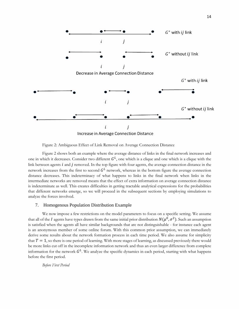
increases or decreases depending on the types of other agents. This is summarized in the following theorem.
THEOREM 2:
Suppose all agents have a capacity of 1. If a link between agents 𝑖 and 𝑗 is removed from 𝐺𝐿, then the distance
of the links of 𝑖 and 𝑗 must increase if they are still linked. The average distance of all links in the network could
either decrease or increase.
14
Figure 2: Ambiguous Effect of Link Removal on Average Connection Distance
Figure 2 shows both an example where the average distance of links in the final network increases and
one in which it decreases. Consider two different 𝐺𝐿, one which is a clique and one which is a clique with the
link between agents 𝑖 and 𝑗 removed. In the top figure with four agents, the average connection distance in the
network increases from the first to second 𝐺𝐿 network, whereas in the bottom figure the average connection
distance decreases. This indeterminacy of what happens to links in the final network when links in the
intermediate networks are removed means that the effect of extra information on average connection distance
is indeterminate as well. This creates difficulties in getting tractable analytical expressions for the probabilities
that different networks emerge, so we will proceed in the subsequent sections by employing simulations to
analyze the forces involved.
7. Homogenous Population Distribution Example
We now impose a few restrictions on the model parameters to focus on a specific setting. We assume
that all of the 𝐼 agents have types drawn from the same initial prior distribution 𝑁(𝜇0, 𝜎2). Such an assumption
is satisfied when the agents all have similar backgrounds that are not distinguishable - for instance each agent
is an anonymous member of some online forum. With this common prior assumption, we can immediately
derive some results about the network formation process in each time period. We also assume for simplicity
that 𝑇 = 1, so there is one period of learning. With more stages of learning, as discussed previously there would
be more links cut off in the incomplete information network and thus an even larger difference from complete
information for the network 𝐺𝐿. We analyze the specific dynamics in each period, starting with what happens
before the first period.
Before First Period

15
Notice that in this setting only agents with a true type that is within 𝛿𝑖 of the population mean 𝜇0 will
form any initial links. Agents that fail this criteria know that their true type is too far away from the average
expected type, and so will not want to experiment with any other agent. We call such agents self-isolated agents.
Such agents will never form any links and remain as singletons in all subsequent time periods. The failure of
these self-isolated agents to form links may be undesirable from a social standpoint, as there is a positive
probability that another agent was within 𝛿𝑖 of a self-isolated agent, and a link could have been sustained
between that pair. But due to the initial beliefs of these self-isolated agents, they do not wish to experiment and
find other agents like themselves.
Agents that do have a true type within 𝛿𝑖 of 𝜇0 will form links with all other such agents. We call these
agents participating agents, because they are close enough to the population mean that they expect a high chance
of linking with a partner similar to themselves. At the start of the first period, the network 𝐺0 will be a clique
composed of participating agents, with self-isolated agents as singletons.
A special case that we can consider is when all agents have the same homophily preferences and use
the same linking cutoff 𝛿. In this case we will also be able to analyze comparative statics of the model with
respect to the size of this cutoff. Note that the 𝛿 in this case can be interpreted as a social norm, since a larger
𝛿 means that all agents are more tolerant of those that are different from themselves while a smaller 𝛿 means
that the agents are less tolerant. Our first result, Lemma 3, shows that more tolerant social norms will lead to
more participating agents and less isolation from the network. The lemma follows from the discussion above.
Thus to prevent isolation of agents, a more tolerant social norm should be adopted initially.
LEMMA 3:
The larger the size of 𝛿, the smaller the set of self-isolated agents and the larger the set of participating agents
in the network.
First Period Dynamics
During the first period, signals will be sent and the agents will update their beliefs based on these
signals. For each neighbor, an agent will stay linked only if the expected belief about that agent’s 𝜇𝑗1 is within
𝛿𝑖 of their own type. The probability of this occurring is given in Lemma 1 as:
𝑃(𝑆𝑖𝑗1 |𝜃𝑖, 𝜃𝑗, 𝛿𝑖) = Φ (−
𝜏0(𝜇0 − 𝜃𝑖 − 𝛿𝑖)
√𝜏𝑟+ √𝜏𝑟(𝜃𝑖 + 𝛿𝑖 − 𝜃𝑗))
− Φ (−𝜏0(𝜇0 − 𝜃𝑖 + 𝛿𝑖)
√𝜏𝑟+ √𝜏𝑟(𝜃𝑖 − 𝛿𝑖 − 𝜃𝑗))
Note that based on the initial linking actions that form 𝐺0, we know that 𝜃𝑖 and 𝜃𝑗 are separated by at
most 𝛿𝑖 + 𝛿𝑗 due to the triangle inequality. We do not assume that the agents take this into account when Bayes
updating; instead, we assume that the agents Bayes update merely use the signal that they receive. However,
when calculating the ex ante probability that any network emerges at the end of period 1, this fact should be
taken into account. The ex ante probability that any link between agents 𝑖 and 𝑗 exists at the end of period 1 will
be given by:
∫ ∫ 𝑃(𝑆𝑖𝑗1 |𝜃𝑖, 𝜃𝑗, 𝛿𝑖) ∗ 𝑃(𝑆𝑗𝑖
1|𝜃𝑗, 𝜃𝑖, 𝛿𝑗)
𝜇0+𝛿𝑖
𝜇0−𝛿𝑖
𝑑Φ(𝜃𝑖)𝑑Φ(𝜃𝑗)
𝜇0+𝛿𝑗
𝜇0−𝛿𝑗

16
After First Period Dynamics
After the first period, agents that are linked in 𝐺1 will learn all remaining information about each other
and find out each other’s true type. The probability that a link remains is 1 if the agents are within 𝛿𝑖𝑗 ≡
min(𝛿𝑖 , 𝛿𝑗). Therefore, we can get the ex ante probability that a link remains between agents 𝑖 and 𝑗 in the
complete information network as:
∫ ∫ 𝑃(𝑆𝑖𝑗1 |𝜃𝑖, 𝜃𝑗, 𝛿𝑖) ∗ 𝑃(𝑆𝑗𝑖
1|𝜃𝑗, 𝜃𝑖, 𝛿𝑗)
min(𝜃𝑗+𝛿𝑖𝑗,𝜇0+𝛿𝑖)
max(𝜃𝑗−𝛿𝑖𝑗,𝜇0−𝛿𝑖)
𝑑Φ(𝜃𝑖)𝑑Φ(𝜃𝑗)
𝜇0+𝛿𝑗
𝜇0−𝛿𝑗
This probability is strictly smaller than the first period probability, and the network learned information
𝐺𝐿 will be a subnetwork of 𝐺1.
Link Refinement Phase Dynamics
In the second phase, agents that are still linked in 𝐺𝐿 will evaluate their current links on the basis of
capacity constraints. Agents will cut off links if they are over capacity, and a final stable network will develop
as discussed above. Fixing the vector of true types, we can map any network 𝐺𝐿 into a final network 𝐺∗ using
the stable network procedure that was described previously. The ex ante probability of a final network 𝐺∗
occurring can be found by using the above formula to get the probability that a network 𝐺𝐿 and a
corresponding true type vector that leads to 𝐺∗ occurs, and adding up the probabilities of all these networks to
get the probability of 𝐺∗.
We wish to make comparisons between the final network 𝐺∗ that develops from the learning process
against a network that would develop if information were complete. Notice that the effect of the learning
process is to make some links unviable. That is, there are some pairs of agents whose true types were closer
than 𝛿𝑖𝑗 and may have wanted to link in the complete information network, but due to errors in the learning
process ended up not being linked in 𝐺𝐿. In this sense, the learned information network 𝐺𝐿 will always be a
subnetwork of the complete information network 𝐺𝐶, which is defined as the network between all pairs of
agents with types closer than 𝛿𝑖𝑗 ignoring capacity constraints.9 Thus we want to study the effect of a removal
of links from 𝐺𝐶 on the final network 𝐺∗, where the removal is due to errors in learning in the experimentation
phase. We will do so via Monte Carlo simulations. We note that numerical integration techniques can also be
used to get these results, since we have the analytical expressions above.
8. Numerical Simulations and Asymptotic Theorems
In this section we will present several figures showing the results of numerical simulations for the
homogeneous population network. Refer to the technical appendix for exact details on how the simulations are
run as well as specific definitions of all the metrics that are used. We assume that there are 10 agents that all
come from a homogeneous population, and we show the impact of a change in social tolerance on various
metrics of the network. Figure 3 shows the Jaccard distance between the final network with complete
information, which we call 𝐺𝐶∗, and final network with incomplete information 𝐺∗ as a function of the social
tolerance. The Jaccard distance measures the difference in the links of the complete information and the
incomplete information network. There are two different forces that affect the Jaccard distance as social
tolerance increases. First a larger social tolerance tends to cause more possible links, allowing for more places
9 This is the network that would be formed if all agents knew all other agents’ types perfectly initially and there were no capacity constraints.

17
in which the complete and incomplete information networks differ. This effect serves to increase the Jaccard
distance. On the other hand, a larger social tolerance means that learning is more accurate, and this effect serves
to decrease the Jaccard distance. Interestingly, the simulations show that there is a maximum value of this
distance at an intermediate level of social tolerance, and the distance goes to zero as the social tolerance becomes
very large or very small.
We can prove that the learned information networks and the complete information network will with
high probability be very similar if the tolerance is either very small or very large. If the tolerance is very small,
no links form in either case. If the tolerance is very large, all links form initially and few are broken. The
following result formalizes this intuition.
THEOREM 3:
As 𝛿 → ∞ or 𝛿 → 0, the probability that the learned information network 𝐺𝐿 is the same as the complete
information network 𝐺𝐶 converges to 1 and the Jaccard distance between the final network with complete
information 𝐺𝐶∗ and final network with incomplete information 𝐺∗ converges to 0 in probability.
PROOF:
In the limit as the tolerance goes to zero, we will have a completely disconnected network for any ex post
realization of types under both complete and incomplete information, so the result holds. In the limit as the
tolerance goes to infinity, the amount of learning becomes perfect, and so links in 𝐺𝐿 will almost surely be the
same as the links in 𝐺𝐶. The Jaccard distance also converges to zero in probability as a direct result of the fact
that in both limits the links in 𝐺𝐿 and 𝐺𝐶 will be the same almost surely. Thus the capacity constraints will be
applied in the same way for both networks, resulting in the same final networks.
∎

18
Figure 3: Jaccard Distance between the complete and incomplete information network as a function of the
social tolerance
We next analyze how the average number of links per agent in the final network 𝐺∗ depends on the
social tolerance. It might seem intuitive that as social tolerance increases, the number of links per agent should
also increase. However, this may not be true for every realization of signals and types. To see why, consider
two social tolerance levels, 𝛿′ < 𝛿. It is true that the set of links in 𝐺𝐿 under 𝛿′ must be a superset of the set
of links under 𝛿 for every realization. (This is because if a link would have been cut off under 𝛿′, it would have
been cut off under 𝛿 as well.) However, the capacity constraints, which govern which links in 𝐺𝐿 survive in the
passage to the final network 𝐺∗, may interfere with additional links being passed to the final network.
This is highlighted in the example in Figure 4, which the potential effects of adding links to 𝐺𝐿 .
Suppose that all agents shown in these figures have a capacity of one. We note that agents 𝑖 and 𝑗 have the
shortest social distance among all agents, and so would form a link in the final network if they have a link in
𝐺𝐿. In addition, a link is not possible between agents 𝑙 and 𝑚 in either the top or bottom 𝐺∗ network since
such a link is not present in either 𝐺𝐿 network. In the top 𝐺𝐿 network a link is not present between agents 𝑖
and 𝑗, and so agent 𝑖 links with agent 𝑙, while agent 𝑗 links with agent 𝑚 in that 𝐺∗. In the bottom 𝐺𝐿 network
this link is present, and so agent 𝑖 links with 𝑗, but agents 𝑙 and 𝑚 do not link. Then in the top 𝐺∗ final network
there will be two links formed, but in the bottom 𝐺∗ final network only a single link will be formed. Thus the
number of links formed in the final network reduces given an increase in the number of links in 𝐺𝐿.

19
Figure 4: Decrease in total number of links in 𝐺∗ as a link between the agents 𝑖 and 𝑗 is added to 𝐺𝐿
Since it is possible for an increase in links in 𝐺𝐿 to decrease the links in 𝐺∗, the ex post effect of a
higher social tolerance 𝛿 is ambiguous. Figure 5 suggests however that the average effect is to increase the total
links in the network. Thus the increase in the links of 𝐺𝐿 dominates any potential issues that the implementation
of the capacity constraints could cause.
Figure 5: Average Number of Links Per Agent in Final Network Based on Social Tolerance
Figure 6 shows the average total distance of links per agent as a function of the social tolerance. This
is defined as the average of the sum of the distance in types between each agent and all its neighbors. It can be

20
observed that as the social tolerance increases, the number of links increases as well. However, the normalized
average distance, equal to the sum distance divided by the social tolerance, increases to a maximum and then
decreases. The average distance is zero at low 𝛿 since links become very unlikely, and the normalized distance
is also zero which shows that the rate at which the average distance goes to zero is faster than the rate at which
𝛿 goes to zero. Thus it should be increasing in the beginning. However, at high 𝛿 the sum distance should
saturate since greater social tolerance does not have an impact once the capacity level is hit.
Figure 6: Average Distance in Incomplete Information Final Network as a Function of Social Tolerance
We now show the effect of social tolerance on clustering within the network. Clustering is a measure
of how frequently a neighbor of a node is connected with other neighbors of the same node, or how often
friends of friends are connected. We analyze the average of the local clustering coefficient of all the nodes of
the network. The local clustering coefficient of a node is equal to the proportion of links that exist among the
subgraph of that node and its direct neighbors divided by the total number of links that are possible within this
subgraph.
Figure 7 shows the difference in the average local clustering coefficient between the final complete
information network 𝐺𝐶∗ and incomplete information network 𝐺∗. The complete information network always
exhibits greater clustering than the incomplete information network. This is due to the fact that links are more
likely to be dropped in the learning process under incomplete information. However, when the social tolerance
is very high or low, the difference goes to zero, which is in line with the above simulation showing that the
Jaccard distance also goes to zero as the social tolerance gets very large or small. In fact this is a direct corollary
of Theorem 3 above. Overall the results show that the effect of incomplete information is to lower the overall
level of clustering in the network, which counteracts the increase in clustering that homophily tends to bring.

21
Figure 7: Difference in Local Clustering as a Function of Social Tolerance
9. Extensions
Extreme Agent Networks
An interesting setting to analyze is when most of the agents have types that are very close together, but
a few agents exhibit extreme types. For instance, we might have a single central group (e.g. a moderate political
party) with fringe groups (e.g. extreme factions) on the sides. The network would represent the links that are
formed by such political groups, and our results would show when extreme factions can form links with the
center versus being isolated. We can formalize this by assuming that there are 𝐾 central agents, whose types lie
within the interval [𝛼, 𝛽], where the length of the interval is equal to 𝑑, and 𝐼 − 𝐾 extreme agents, whose types
lie outside of this interval and a distance of at least 𝑑 away from both endpoints 𝛼 and 𝛽, i.e. within the interval
(−∞, 𝛼 − 𝑑] ∪ [𝛽 + 𝑑, ∞). This ensures that all the agents of non-extreme types would prefer to link with
any other agents of a non-extreme type than an extreme agent. Figure 8 shows an example of such a network
with two extreme agents.

22
Figure 8: Example of Extreme Networks
When can an extreme agent connect with a central agent? First it is necessary for all central agents to
have large enough social tolerances that they are willing to connect with the extreme agents. Even if this
condition holds, there must still be a central agent that is under capacity after considering linking with all other
central agents, since we have assumed that the extreme agents are all farther away from the central agents than
any central agent is from another central agent. If there is a central agent that is under capacity after considering
all other central agents, we say that there exists a central agent with an available link. We can prove a result about
when such an event is possible and when it will not be possible.
THEOREM 4:
Suppose 𝛿 > 𝑑. If the capacity is 1 for the central agents then there will be 1 available link if the number of
central agents, 𝐾, is odd and no available links if it is even. If the capacity is 𝐾 − 1 then there will be no available
links. For all other capacity values, there is always a positive probability that a final network emerges in which
there are available links.
PROOF:
For the first result when the capacity is equal to 1, notice that by the assumption that the types of the extreme
agents are all farther away than the maximum possible type difference of the central agents, all the central agents
will link with each other first before linking with an extreme agent. If there are an even number of central agents
then the central agents will all form pairs with each other, resulting in no available links. If there are an odd
number of extreme agents, then there will be one central agent without a partner, and thus 1 available link.
If the capacity is equal to 𝐾 − 1, then the only possible network for the central agents is a clique in which all
the central agents are linked with each other. This is because no matter what the true types of the central agents
are, given the capacity value they will be able to link with every other central agent. After doing so, there will
be no available links left over for the extreme agents.
Finally suppose the capacity is something other than the above two values. If the capacity is greater than or
equal to 𝐾, there will always be available links as even after forming a clique with other central agents each
central agent will still not be at capacity. Suppose then that the capacity is strictly less than 𝐾 − 1 and strictly
larger than 1. We show that there exist networks that emerge with positive probability in which the central
agents have available links.
First assume that the number of central agents 𝐾 is not divisible by 𝑐 + 1. In such a case, let 𝑚 be the greatest
integer such that 𝑚(𝑐 + 1) < 𝐾, and let 𝑟 = 𝐾 − 𝑚(𝑐 + 1). We give a distribution of real types for the central
agents such that the resulting final network will have an available link if 𝐺𝐿 is a clique amongst the central
agents, which happens with positive probability. Separate 𝑚(𝑐 + 1) of the central agents into 𝑚 groups of 𝑐 +
1 agents. Within each group, the agents can be made to be connected in a clique with all the other group

23
members if the type distance between the two greatest separated members of that group is smaller than the
type distance of any member of that group to the closest type member of any other group. Thus there is a
realization of types such that all the 𝑚 groups are composed of cliques. Now consider the remaining 𝑟 agents
that were not placed in a clique. Since all the other agents outside of these 𝑟 agents are already at capacity, and
given that 𝑟 < 𝑐 − 1, it is not possible for these 𝑟 agents can reach capacity only by linking with each other.
Therefore there must be an available link to an extreme agent.
Next suppose that 𝐾 is divisible by 𝑐 + 1. Suppose that 𝐾 is not divisible by 2𝑐, and let 𝑛 be the greatest
integer such that 𝑛(2𝑐) < 𝐾. Let 𝑟′ = 𝐾 − 𝑛(2𝑐), and suppose for now that 𝑟′ ≠ 𝑐 + 1. Take 𝑛(2𝑐) of the
agents and divide them into 𝑛 groups of 2𝑐 agents each. We show that within each group the agents can be
made to reach capacity. This can be done by first assuming that the agents within each group are closer to each
other in type than they are to any other agent of any other group. Take the 2𝑐 agents in each group and further
divide them into two subgroups of 𝑐 agents each. If within each subgroup the types of the 𝑐 agents are closer
to each other than to any member of the other subgroup, the agents in each subgroup will form a clique with
each other, and they will all be 1 link under capacity afterwards. Then, suppose that for concreteness the agents
in the second subgroup all have types greater than the agents of the first subgroup. To fill their capacities, the
agents in the first subgroup will link with the agents in the second subgroup, starting with the greatest in type
agent of the first subgroup and the smallest in type agent of the second subgroup, then the second greatest
agent of the first subgroup and the second smallest agent of the second subgroup, and so on until all the agents
reach their respective capacities.
Suppose that 𝑟′ < 𝑐 + 1. Then the remaining 𝑟′ agents, who can only form links with each other, will be unable
to form enough links to satisfy their capacities and so there will be an available link. Next suppose that 𝑟′ >
𝑐 + 1. In this case we can split off 𝑐 + 1 agents from this set of remaining agents and have them form a clique.
The agents that were not split off will number less than 𝑐 + 1 and so be unable to fulfill their capacities,
resulting in an available link.
Now suppose still that 𝐾 is divisible by 𝑐 + 1 and not 2𝑐, but now the remainder 𝑟′ defined above is equal to
𝑐 + 1. In this case, the above method can be modified to still produce an available link. Take (𝑛 − 1)(2𝑐) of
the central agents and divide them into 𝑛 − 1 groups of 2𝑐 agents, and take 2(𝑐 + 1) of the other central
agents and divide them into two groups of 𝑐 + 1 agents. Following the same procedure as above, the agents
within each group can be made to reach capacity. Afterwards, there will be 𝑐 − 1 agents that were not placed
into a group, and these 𝑐 − 1 agents cannot reach capacity by linking only with themselves and so there must
be an available link.
Finally, suppose that 𝐾 is divisible by both 𝑐 + 1 and 2𝑐 . Let 𝑛 =𝐾
2𝑐. A similar method as above can be
adopted. Take (𝑛 − 1)(2𝑐) of the central agents and divide them into 𝑛 − 1 groups of 2𝑐 agents, and take
(𝑐 + 1) of the other central agents and form a clique with these agents. All the agents that were chosen in this
way can be made to hit capacity, and there will be exactly 𝑐 − 1 leftover agents. These 𝑐 − 1 agents cannot hit
capacity only by linking amongst themselves, and so there will be an available link.
∎
This result is interesting in that it predicts different behaviors of the final network depending on the
precise number of agents as well as the capacity. If the capacity is very low and equal to 1, there will be no or
very few available links, and if the capacity is large and equal to 𝐾 − 1 there will be no available links. For all
other capacity values there may be more available links possible. We test this result via simulations. First we

24
assume that there are 7 central agents with prior distributions drawn from a 𝑁(10, .01) distribution, and 2
extreme agents, one from a 𝑁(9, .01) distribution and one from a 𝑁(11, .01) distribution. (We use normal
distributions for greater tractability in the simulations, but with low initial variances the two settings should be
similar, as with high probability all the central agents will link with each other before linking with an extreme
agent.) We assume that the tolerance is very large, equal to 10, such that the extreme agents will still connect
with each other even if they cannot connect with a central agent. We vary the capacity of the agents from 1 to
7, and we plot the average number of links for the two extreme agents as a function of the capacity. The results
are shown in Figure 9.
Interestingly, the simulation shows that the average number of links exhibits strong non-monotonicity
depending on the capacity. The average number of links increases at first, but then decreases when capacity
gets larger with a minimum at 6. The capacity of 6 is a special value because it represents the capacity at which
the central agents will form a clique with high probability and the extreme agents can only link with each other.
However when the capacity is 7, now each central agent will have one available link so the extreme agents can
link to each central agent for sure.
Figure 9: Average Links of Extreme Agents as a Function of Capacity with Seven Central Agents
We repeat the same simulation but we add an extra central agent so that there are now an even number
of central agents. This is shown in Figure 10. Fitting in line with our earlier results, the pattern is still non-
monotonic and changes greatly with the capacity. It increases somewhat initially and then decreases at the
capacity of 7, which is the capacity at which all central agents are likely to be connected in a clique without
spots for the extreme agents. It then increases greatly at the capacity of 8 since all the central agents will now
have at least 1 open spot. The non-monotonic nature of the graph shows the fragility of these networks. Overall

25
the main takeaway is that extreme agent networks can be very sensitive to the precise specifications, as slight
changes in capacities can result in drastically different outcomes in the network structure.10
Figure 10: Average Links of Extreme Agents as a Function of Capacity with Eight Central Agents
We repeat the above simulations, but this time with a larger number of agents, to see what types of
trends manifest as the set of agents becomes larger. Figure 11 shows the average number of links when there
are 50 and 51 central agents respectively. A number of features stand out. First, both graphs are much smoother
than the case with very few agents, and display a notable trend which is an initial increase to a peak followed
by a decrease. The graphs are also much more similar to each other than is the case with only 7 or 8 agents, as
the peaks and valleys of the graphs occur at very similar places. Finally, the overall trend of the graphs indicates
that extreme agents are initially helped by the central agents having a higher capacity, but eventually hurt as the
capacity of the central agents becomes too large. Then when the capacity no longer binds, which occurs at the
values of 50 and 51 respectively, the extreme agents are once again able to form many links.
10 We note that the capacity is changing simultaneously for all agents, so in that sense any change in the capacity level may be expected to have a significant effect. If the network has many central and extreme agents and the capacity was only changed for a few agents, then the impact should be relatively minor.

26
Figure 11: Average Links of Extreme Agents as a Function of Capacity with 50 and 51 Central Agents
Bimodal Distribution
We now repeat the analysis above using a bimodal normal distribution in order to test the robustness
of our results. The previous simulation analysis will be redone with a bimodal normal distribution, with a 50%
weight on a 𝑁(10,1) distribution, and a 50% weight on a 𝑁(7,2) distribution. A nice property of a bimodal
normal distribution is that the Bayesian updating remains computationally simple. Since there is a one half
probability of coming from the first distribution and a one half probability of coming from the second
distribution, the agent beliefs at each time step can be computed twice assuming that each one of the
distributions is correct. This updating process utilizes the tractable Bayesian updating formula for normal
distributions, and the actual belief at each time step will be a weighted average of these two beliefs. The resulting
graphs show similar general features as in the original unimodal normal distribution case, confirming the
robustness of the initial results.
Figure 12 shows the Jaccard distance between the final complete and incomplete network, similar to
Figure 3. As in that figure, the Jaccard distance is zero or infinity at large or small social distances, and reaches
a single peak at an intermediate value. Although the shape is very similar, one difference is that the social
tolerance level where the Jaccard distance is the greatest is at a larger social tolerance level than in the unimodal
distribution. In addition, the maximum Jaccard distance is also lower.

27
Figure 12: Jaccard Distance between the final complete and incomplete information network with bimodal
distribution
Figure 13 shows the average number of links in the final incomplete information network at different
social tolerance levels with the bimodal distribution. Once again the figure looks very similar to the previous
Figure 5. There is an S shape with the average number of links increasing sharply at first and then plateauing
after the tolerance becomes large. The plateau level is very similar to that of Figure 5, but the inflection point
is at a higher social tolerance level than before.
Finally we note that analogues of Figures 6 and 7 showing the average total distance and the difference
in local clustering between the final complete and incomplete information networks can also be computed for
the bimodal distribution. Like the other figures the resulting graphs look very similar, confirming the robustness
of these results as well, and we avoid including them for the sake of brevity.
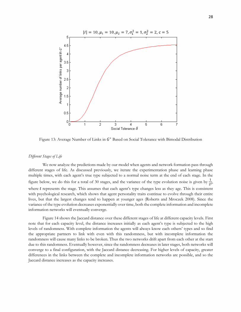
28
Figure 13: Average Number of Links in 𝐺∗ Based on Social Tolerance with Bimodal Distribution
Different Stages of Life
We now analyze the predictions made by our model when agents and network formation pass through
different stages of life. As discussed previously, we iterate the experimentation phase and learning phase
multiple times, with each agent’s true type subjected to a normal noise term at the end of each stage. In the
figure below, we do this for a total of 30 stages, and the variance of the type evolution noise is given by 1
2𝑡,
where 𝑡 represents the stage. This assumes that each agent’s type changes less as they age. This is consistent
with psychological research, which shows that agent personality traits continue to evolve through their entire
lives, but that the largest changes tend to happen at younger ages (Roberts and Mroczek 2008). Since the
variance of the type evolution decreases exponentially over time, both the complete information and incomplete
information networks will eventually converge.
Figure 14 shows the Jaccard distance over these different stages of life at different capacity levels. First
note that for each capacity level, the distance increases initially as each agent’s type is subjected to the high
levels of randomness. With complete information the agents will always know each others’ types and so find
the appropriate partners to link with even with this randomness, but with incomplete information the
randomness will cause many links to be broken. Thus the two networks drift apart from each other at the start
due to this randomness. Eventually however, since the randomness decreases in later stages, both networks will
converge to a final configuration, with the Jaccard distance decreasing. For higher levels of capacity, greater
differences in the links between the complete and incomplete information networks are possible, and so the
Jaccard distance increases as the capacity increases.

29
Figure 14: Jaccard distance between complete and incomplete information network for different stages
of life and at different capacity levels.
Figure 15 shows the Jaccard distance over different stages of life at different social tolerance levels.
For all social tolerance levels, the shape of the curve is similar to the shapes in Figure 14 with a single peak and
then a decline. However, the Jaccard distance does not change monotonically with the social tolerance as it
does with the capacity. The lowest social tolerance of . 1 gives the lowest Jaccard distance throughout, but the
highest social tolerance of 1 starts and ends at an intermediate Jaccard distance, although it does feature the
largest peak Jaccard distance. This non-monotonicity of the Jaccard distance with respect to social tolerance
mirrors the non-monotonicity that is present in Figure 3. At larger social tolerance levels more links are possible
so the potential differences in the links is greater, but learning also becomes more accurate which tends to
reduce the differences between complete and incomplete information. Even with multiple stages of life, an
analogue of Theorem 3 holds so that as the social tolerance becomes very large or very small the Jaccard
distance must approach zero at all stages of life.

30
Figure 15: Jaccard distance between complete and incomplete information network for different stages
of life and at different social tolerance levels.
10. Conclusion
In this paper we formulated a model to capture the impact of homophily on the interaction between
learning and network formation. In this model, agents learn about each other through mutual interactions;
homophily leads them to maintain connections only with agents that are (learned to be) similar to them. Our
results show that incomplete information leads to lower clustering than would arise under complete information.
The reason is that due to errors in the learning process, agents may not actually find out which others are most
like them, so with some probability agents may choose neighbors who are less similar to themselves than the
neighbors they would choose when information is complete. The extent of the difference between the complete
and incomplete information network depends heavily on social tolerance; surprisingly, the difference goes to
zero as the social tolerance becomes very small or very large. When we incorporate multiple stages of life, we
see that the difference between the complete and incomplete information networks is initially very large, but
eventually decreases over time.
Many interesting extensions suggest themselves. One obvious extension is to allow the signals that the
agents send to their neighbors in each time period to be correlated (rather than independent). Such correlation
may lead to greater clustering, because when one neighbor receives an extreme signal and so severs a link, other
neighbors will be more likely to receive an extreme signal and also sever the link. Another obvious extension is
to allow for indirect learning via friends of friends. If agent A is connected to agent B and agent B is connected
to agent C, then agent A might learn about agent C indirectly -- even if they are not directly linked (although

31
presumably indirect learning would be noisier). Indirect learning might also lead to greater levels of clustering,
as friends of friends are now more likely to find out about each other and hence connect.
Potentially interesting – and realistic -- extensions of the multiple stages of life model would be to allow
for changes in agent characteristics across different stages of life. For instance, agents might become either
more or less tolerant as they age, which could have a large impact on the Jaccard distance between complete
and incomplete information networks: if agents begin life very tolerant but become less tolerant over time, the
Jaccard distance might increase as agents age, rather than decreasing. Changes in tolerance – and in other
characteristics – might be exogenous, but endogenous changes – changes that are influenced on the basis of
links that are formed – seem especially interesting and important.
Finally, it would be very interesting to use data from real world networks to test the predictions of the
model. For instance, we might use data of networks of coauthors in academic journals to see how ties between
authors evolve over time. In this setting the type could represent the academic interests of the author and the
signals could be previous publications of the authors. Alternatively, we might test the predictions of our model
in online social networks (in which type would represent the interests of the agents and the signals would be
the messages that agents send to each other) to see how links between friends change as agents learn and
interact with each other.

32
Monte Carlo Simulation Technical Appendix
We perform Monte Carlo simulations of the network learning and formation process to derive properties of
the resulting networks. Fixing the set of 𝐼 agents and the normal prior distributions 𝑁(𝜇𝑖0, 𝜎𝑖
2), for each run of
the simulation we take a draw of true agent types from the prior distribution. We then form the initial network
𝐺0 based on the tolerances 𝛿𝑖 and these true types. Using this network 𝐺0, we simulate the signals that each
agent sends in each period of the experimentation phase. All the simulations in the paper use one period for
the experimentation phase, and thus one signal is sent per agent during experimentation. Greater numbers of
periods will tend to increase the differences with the complete information network. From the agent signals,
we can compute the learned information network 𝐺𝐿 that forms using the agent linking rules.
For each 𝐺𝐿 we then apply the capacity constraints using the stable network procedure described in the paper
to get the final network 𝐺∗. Thus in each run of the simulation we can arrive at a final network 𝐺∗.
Using the same types that were drawn initially, we can also derive the resulting complete information network
𝐺𝐶 by computing which agents wish to link with each other given the social tolerance thresholds. We then
apply the capacity constraints onto the network to get the final complete information network 𝐺𝐶∗. From all the
runs of the distribution, we can then get estimates of the probability that each final incomplete information
network 𝐺∗ and complete information network 𝐺𝐶∗ will form.
From the distributions of 𝐺∗ and 𝐺𝐶∗ obtained through the runs of the simulation, we can analyze different
parameters of interest, which are defined below.
Definitions:
Average number of links of each agent
From the numerical analysis, we get the probability of the network evolving into each possible final network.
Then we take the number of links each agent has in each final network, and we weight it by the probability that
final network occurs, to get the average number of links each agent has.
Jaccard Distance
For a fixed final complete information and final incomplete information graph, we count the number of
differences in the adjacency matrices of the two graphs and sum them up. We take the average of this sum over
all runs of the Monte Carlo simulations.
Average Total distance of links of each agent
The sum of the distance of all the links each agent has in each final network. We take the average over the
agents.
Local Clustering Coefficient
The average of the local clustering coefficient of all the nodes of the network. The local clustering coefficient
of a node is equal to the proportion of links that exist among the subgraph of that node and its direct neighbors
divided by the total number of links that are possible within this subgraph.

33
REFERENCES
[1] Acemoglu, D., Dahleh, M. A., Lobel, I., & Ozdaglar, A. (2011). Bayesian learning in social networks. The
Review of Economic Studies, 78(4), 1201-1236.
[2] Akerlof, G. A. (1997). Social distance and social decisions. Econometrica: Journal of the Econometric
Society, 1005-1027.
[3] Baccara, M., & Yariv, L. (2015). Choosing Peers: Homophily and Polarization in Groups.
[4] Bala, V., & Goyal, S. (2000). A noncooperative model of network formation. Econometrica, 68(5), 1181-
1229.
[5] Bramoullé, Y., Currarini, S., Jackson, M. O., Pin, P., & Rogers, B. W. (2012). Homophily and long-run
integration in social networks. Journal of Economic Theory, 147(5), 1754-1786.
[6] Currarini, S., Jackson, M. O., & Pin, P. (2009). An economic model of friendship: Homophily, minorities,
and segregation. Econometrica, 77(4), 1003-1045.
[7] Fu, F., Nowak, M. A., Christakis, N. A., & Fowler, J. H. (2012). The evolution of homophily. Scientific
reports, 2.
[8] Galeotti, A., & Goyal, S. (2010). The law of the few. The American Economic Review, 1468-1492.
[9] Gauer, F., & Landwehr, J. (2015). Continuous homophily and clustering in random betworks. Mimeo.
[10] Golub, B., & Jackson, M. O. (2010). Naive learning in social networks and the wisdom of crowds.
American Economic Journal: Microeconomics, 112-149.
[11] Golub, B., & Jackson, M. O. (2012). How homophily affects the speed of learning and best-response
dynamics. The Quarterly Journal of Economics, 127(3), 1287-1338.
[12] Halberstam, Y., & Knight, B. (2015). Homophily, group Size, and the diffusion of political information
in social networks: evidence from Twitter. Mimeo.
[13] Iijima, R., & Kamada, Y. (2014). Social distance and network structures. Mimeo.
[14] Jackson, M. O. (2008). Average distance, diameter, and clustering in social networks with homophily.
In Internet and Network Economics (pp. 4-11). Springer Berlin Heidelberg.
[15] Jackson, M. O., & Wolinsky, A. (1996). A strategic model of social and economic networks. Journal of
economic theory, 71(1), 44-74.
[16] Johnson, C., & Gilles, R. P. (2000). Spatial social networks. Review of Economic Design, 5(3), 273-
299.
[17] Kossinets, G., & Watts, D. J. (2006). Empirical analysis of an evolving social network. Science,
311(5757), 88-90.
[18] Kovanen, L., Kaski, K., Kertész, J., & Saramäki, J. (2013). Temporal motifs reveal homophily, gender-
specific patterns, and group talk in call sequences. Proceedings of the National Academy of
Sciences, 110(45), 18070-18075.

34
[19] Laumann, E. O., & Senter, R. (1976). Subjective social distance, occupational stratification, and forms
of status and class consciousness: A cross-national replication and extension. American Journal
of Sociology, 1304-1338.
[20] Marsden, P. V. (1988). Homogeneity in confiding relations. Social networks, 10(1), 57-76.
[21] McPherson, M., Smith-Lovin, L., & Cook, J. M. (2001). Birds of a feather: Homophily in social networks.
Annual review of sociology, 415-444.
[22] Roberts, B. W., & Mroczek, D. (2008). Personality trait change in adulthood. Current directions in
psychological science, 17(1), 31-35.
[23] Watts, A. (2001). A dynamic model of network formation. Games and Economic Behavior, 34(2), 331-
341.