Embed Size (px)
Citation preview
Fashion and Homophily∗
Bo-Yu Zhang† Zhi-Gang Cao ‡ Cheng-Zhong Qin§
Xiao-Guang Yang¶
May 3, 2013
Abstract
Fashion, as a “second nature” to human being, plays a quite non-trivialrole not only in economy but also in many other areas of our society, in-cluding education, politics, arts, and even academics. We investigate fashionthrough a network game model, which is referred to as the fashion game,where there are two types of agents, conformists and rebels, who are allo-cated on a network. Each agent has two actions to choose, and interacts onlywith her neighbors. Conformists prefer to match the majority action amongher neighbors while rebels like to mismatch. Theoretically, the fashion gameis a network extension of three elementary games, namely coordination game,anti-coordination game, and matching pennies. We are especially interestedin how social interaction structures affect the evolution of fashion. The con-clusion is quite clean: homophily, in general, inhibits the emergence of fashioncycles. To establish this, two techniques are applied, i.e. the best responsedynamics and a novel partial potential analysis.
∗This is a sister working paper with: Zhi-gang Cao, Cheng-zhong Qin, Xiao-guang Yang, Bo-yuZhang, A heterogeneous network game perspective of fashion cycle. The research is supported bythe 973 Program (2010CB731405) and National Natural Science Foundation of China (71101140).We gratefully acknowledge helpful comments from Xujin Chen, Zhiwei Cui, Xiaodong Hu, WeidongMa, Changjun Wang, Lin Zhao, and Wei Zhu.
†Department of Mathematics, Beijing Normal University, Beijing, 100875, China. Email: [email protected].
‡MADIS, Academy of Mathematics and Systems Science, Chinese Academy of Sciences, Beijing,100190, China. Email: [email protected].
§Department of Economics, University of California, Santa Barbara, CA 93106, USA. Email:[email protected].
¶MADIS, Academy of Mathematics and Systems Science, Chinese Academy of Sciences, Beijing,100190, China. Email: [email protected].
1

Keywords: social value, fashion cycle, homophily, partial potential analy-sis, best response dynamics
JEL Classification Number: A14; C62; C72; D72; D83; D85; Z13
1 Introduction
Although the world’s wealth is distributed quite unevenly, the unprecedentedoverall affluence is an undeniable fact1. For most people living in developedcountries, as well as those in developed areas of developing countries, theirbasic physical needs in life are easily met. They live mainly not for personalcomfort, but for social comfort (Scitovsky, 1986). Consequently, comparedwith physical value, social value becomes a more and more crucial factor whenpeople consider whether to buy a product2 . Suppose there are two kinds ofproducts that have the same functions, similar qualities and performances,but one is very “in” and the other is “out”. Then it is not surprising that thein product can be much more expensive than the out one, because its socialvalue is much higher.
There are several interesting and crucial features possessed by social value,but generally not by physical value. (i) Social value might well be negative3.(ii) The social value of the same product may be extremely different and evenopposite to different people. (iii) The social value one gets from consuminga product is not determined by the product itself or by the the consumer,but mainly by how other people around the consumer view this product, andwhat’s even more interesting, can be greatly affected by what people aroundher consume4.
1Tim Jackson (2009) even argues that it is time to reconsider the definition of prosperity, anda flourishing world without GDP growth is possible (at least in the near future), because we arealready rich enough in materials.
2Another important dimension in the total value of a product is emotional value. The threedimensions reflect the relationships of the consumer between the product, between the society andbetween herself, respectively. See more discussions in van Nes (2010).
3In contrast, almost all products have a positive physical value. This can be proved throughthe fact that the concept of product is identical to goods, and usually bads (say wastes) are notselling products.
4As quoting from Braudel (1714), “Nothing makes nobel persons despise the gilded costume somuch as to see it on the bodies of the lowest men in the world...” (see also Pesendorfer, 1995).Despite most people today, including us, agree that people are born equal and there should not besuch concepts as “nobel people” or “low people”, and despite the fact that the world is becomingflatter and flatter, that similar phenomena still exist widely as to a “tasteful” person, in general,is not so happy to see other people consume the same product as she does. This phenomenonillustrates the three features of social value very well. The same skirt may provide an “untasteful”
2

Social value covers in general“the image of the product, the appreciationby others, the sense of luxury and the provision of status” (van Nes, 2010).However, how bright the image of a product is, whether you can get appreci-ation through consuming this product, and whether it will give you the senseof luxury or the proper social identity, are mostly determined by how otherpeople view this product. The overall consumption related viewpoint or col-lective taste of the society can be summarized very well in the current fashiontrends.
Fashion plays such a key role in producing the total value of a productthat it is ranked second only to technology, because as technology contributesmost to the physical value of a product, fashion contributes most to socialvalue5. The complementary relation between technology and fashion can alsobe observed in a perhaps even more important fact that while technologyaccelerates, and sometimes creates, supply, it is fashion that influences moredirectly on demand, through shaping consumers’ tastes and consequently theirpurchasing behaviors.
In the following two subsections, we shall give a brief discussion on the im-pacts of fashion on environment and economy. These impacts are doubtlesslyenormous. And fashion cycle, the focus of this paper that will be introducedin Subsection 1.3, is also key to the working of these impacts.
1.1 Fashion and environment
People’s discarding behavior is consistent with their pursuing behavior. Whenthey consider whether to discard a product, the reason that it fails to work isbecoming less and less often, and an increasingly frequent reason is that it isnot fashionable any longer6. It has been confirmed by research that for manykinds of products7, a significant proportion of them still function very wellwhen discarded. The chief reason is that they are “out of fashion”. Fashion,“the key hazard for durability of consumer goods”, has been hand in handwith the throwaway culture ever since industrialization (Stahel, 2010).
The most severe criticism on the prevailing throwaway culture is probablythat it is hugely incompatible with sustainable development. Overconsump-
person positive social value and a “tasteful” person negative social value, and the negative feelingof the “tasteful” person is in fact from the behavior of the others.
5Note that this is valid only for consumer goods, not for capital goods. See also the discussionof Stahel (2010), where the term “psychological value” was adopted instead of “social value”.
6In the term of Packard (1963), this reason can be classified into obsolescence of desirability orpsychological obsolescence. See also Cooper (2010). Other reasons include personal life, marketdevelopment, financial situation, etc., see van Nes (2010).
7E.g., furniture and appliances (Anderson, 1999; Cooper and Mayers, 2000), electronic products(Slade, 2006), and most obviously, clothing.
3
tion is the natural result of this culture. Huge amount of unnecessary wastesare produced, limited natural resources are squandered, and the life-spans ofmost consumers goods are extremely short. It may be surprising to most of usto know that few of today’s products last longer than previous ones, despitethe accelerating development of science and technology. An astonishing andironical example is light bulb, which has an intentionally short life-span byproducers. Recall the effort paid by Thomas Edison to invent the first stablelight bulb! The strategy taken by the producers, planned obsolescence, has along history and is widely used (Cooper, 2010). See Slade (2006) for a morecomprehensive historical review. Thus it is believed that sustainable devel-opment will only be possible if the throwaway culture is changed (Cooper,2010).
Producers should take much responsibility for the throwaway culture. Inorder to promote repetitive consumption and thus settle the problem of over-production, producers in the late 19th century of America gradually adopted“a wide range of manufacturing strategies, from branding, packaging, andcreating disposable products, to continuously changing the styles of non-disposable products” (Slade, 2006). Along with them are advertising andmarketing, which are deeply believed to be able to create and shape con-sumption. They worked, and there came along commercial fashion. Variousformats of fashion sprouted. Whichever social class did a consumer belongto, there must be a suitable format for her. From then on, fashion began tobecome a culture, and throwaway a lifestyle.
Nevertheless, consumers are not merely victims, they are not free of crit-icism either. In fact, producers, to a great extent, are only catering to thepsychological and social needs of consumers (see Veblen, 1899; Chai et. al.,2007). We can argue that the evolution of fashion is a result of the “collusion”of producers and consumers, and it is consumers who have the ultimate rulingpower. In this paper, we shall only concentrate on the consumer side of theevolution of fashion.
1.2 Fashion and economy
There are at least two reasons why fashion is important to economy. First ofall, fashion is a huge industry. Despite all the complications to give a satis-factory definition of the fashion industry8, its global market size is estimated
8There are mainly three complications. First, nowadays most consumer products have more orless fashion ingredient and thus it is almost impossible to define a clear border between fashionindustry and non-fashion industry. For one example, people may never agree on whether iPad andiPhone should be classified as fashionable products or not. A similar debatable product in Chinais the “luxury” alcohol Maotai. A second point is that in our daily life, the fashion industry isusually treated equivalent to the industry of costume and clothing. Obviously, it should be much
4
at some $ 200 billion US dollars 9. The importance of fashion industry can befurther justified by the following facts (Okonkwo, 2007): “[fashion industry]is one of the few industrial segments that have remained a constant worldeconomy contributor with an annual growth rate of approximately 20 per-cent. [...] The luxury fashion sector is the fourth largest revenue generator inFrance; and one of the most prominent sectors in Italy, Spain, the USA andthe emerging markets of China and India. The sector is currently one of thehighest employers in France and Italy.”
Second of all, fashion stimulates economic growth. Planned obsolescencehas long been believed by governments as an efficient way to stimulate eco-nomic growth, at least in economic crisis when production fails to be able tocontinue. From the Great Depression to the global recession in 2008, con-sumption stimulating policies, which encouraged consumers to replace stillfunctional products, were introduced to rescue the market (Packard, 1963;Slade, 2006; Cooper, 2010). Fashion, as a constant consumption stimulator,plays a similar role. Although this theory is greatly debatable, it is certainthat the role of fashion on economic growth deserves at least serious study10.
1.3 Fashion cycle
Not only in economy and environment, but also in many other areas of thesociety, say education, politics, art, and even academics, fashion is a factorthat cannot be neglected (Blumer, 1969). Originating in the before industrialsociety almost at the very beginning of civilization, and flourishing in theindustrial society, fashion is now playing a more and more crucial role inalmost every corner of the post industrial society. A recent research showsthat charitable donation among celebrities is also a highly subject of fashion(Schweitzer and Mach, 2008). In fact, as claimed by Svendsen (2006),
“Fashion has been one of the most influential phenomena in West-ern civilization since the Renaissance. It has conquered an increas-ing number of modern man’s fields of activity and has becomealmost ‘second nature’ to us ”.
broader than this. A third point is that it is frequently mixed with the luxury industry.9The data is for luxury industry. See Okonkwo, 2007; See also Euromonitor International:
Global luxury goods overview, June 2011. What’s more, it is estimated that only in US, $ 300billion expenditure are driven by fashion rather than by (physical) need (Yoganarasimhan, 2012b).
10A similar logic is known as the broken window fallacy, which is (in)famous due to the criticismof Bastiat (1850). OECD (1982) recommended that further research be undertaken on a closelyrelated problem, i.e. the macroeconomic effects of longer product life-spans. A recent research byChai et. al. (2007) is on the positive side. Cooper (2010) thinks that the relation is still poorlyunderstood, especially when environmental impacts are also taken into account.
5
Compared to technology, the other main driving force in market and so-ciety, fashion is much more intangible and unpredictable. This is quite un-derstandable, because as technology reflects the ability of the human being,fashion reflects our dreams. As we know, dreams can be quite flexible andadjustable. There is an “arrow” for the development of technology: like time,it keeps advancing. And very few people doubt the positive rule of technology.Despite its enormous impact on market, society and environment, the multi-fold roles that fashion plays are rather complicated. In particular, there isno arrow for its development and we frequently observe the opposite: fashioncycle.
Like economy has ups and downs, fashion comes and goes, and after usuallyan unexpected period of time, it may come back again. This phenomenon,supported by numerous daily observations11, is called fashion cycle. Fashioncycle is usually taken as the most extraordinary and the most “mysterious”part of fashion. It is so crucial to understand fashion that it could be deemedas the “pulse” of it. If fashion were not in constant flux, then its impact onenvironment and economy would have disappeared, because people would notreplace their goods at all, until they are completely worn out.
Not surprisingly, trying to understand the logic of fashion cycle is oneof the key focuses of previous studies (cf. Pesendorfer, 1995; Young, 2001;Yoganarasimhan, 2012a). It is the focus of this paper too. In particular, weshall concentrate on the basic question of what causes fashion cycle.
It is safe to say that fashion cycle is caused ultimately by a combined forceof consumers and producers. However, the concrete process may be quite com-plicated, and the task of theoretical as well as empirical studies is to revealmore details of this process. In the classical model of Pesendorfer (1995), fash-ion cycle is determined and completely controlled by a monopolist producer.In his model, the problem he attacked is not the causes of fashion cycle, buthow to control it optimally. Although the main assumption that everythingis decided by a powerful producer is obviously unrealistic, because very rarelycan a producer be so powerful, this theory provides us new understandings ofthe fashion cycle on the producer side. On the consumer side, motivationally,fashion cycle may come out of the needs for class signaling (Simmel, 1904),wealth signaling (Veblen, 1899), cultural capital signaling (Bourdieu, 1984),taste signaling (Yoganarasimhan, 2012b), or personality signaling (Cao et al.,2013b).
In this paper, we shall provide a new structural factor from the perspectiveof homophily, a concept that will be introduced in Subsection 1.6.
11Anecdotal observations on the existence of fashion cycle, e.g. fashion color and length of girls’skirts, can be found throughout history. However, as pointed out by Yoganarasimhan (2012b),“[...] how to detect fashion cycles in data has not been studied.”
6
1.4 Conformists and rebels
On what is fashionable, interestingly, there are two completely opposite view-points that are both extremely popular. “Wow, Lady Gaga is fashionable!”“This year’s fashion color is black”. In the above expressions, the viewpointsof fashion are quite opposite. In the dictionary of Merriam-Webster, thereare two definitions for fashion, reflecting the two opposite opinions. One isthat “a distinctive or peculiar and often habitual manner or way”, and theother is “a prevailing custom, usage, or style”. This difference also reflectspeople’s various psychological and social needs: different people have differentdesiring (or enduring) levels of to be how different with the others. The modelexplored in this paper is roughly a game played by the preceding two groupsof people in social networks. Following the terms of Jackson (2008), we shallcall the above two kinds of people rebels and conformists, respectively.
Simmel (1904), one of the pioneers in the study of fashion, argued thattwo antagonistic tendencies (imitation and differentiation, union and segre-gation, conformation and deviation etc.) are simultaneously deeply rootedin the soul of every individual. Based on this core logic, he demonstratedeloquently the proposition, which was stated more explicitly a century laterby Svendsen (2006), that fashion is a “second nature” of the human being.What’s more, Simmel claimed that people’s conforming and deviating activi-ties in fashion have a rather stylized pattern, that is, the former tendency isembodied overwhelmingly in lower class people while in upper class people,the latter tendency is dominant. Hence upper class people are fashion leaders(i.e. rebels) and lower class people are fashion followers (i.e. conformists).This theory, also known as the “class differentiation”, is the key premise ofmost later theoretical studies on fashion. In this paper, as in the sister workingpaper, however, we shall not divide people into lower class and upper class,but distinguish them directly into conformists and rebels. This can be takenas a “personality differentiation” theory. See more discussions in Cao et al.(2013b).
We shall also assume that there is no product innovation. This can bedeemed as an investigation of what happens during a relatively steady time,i.e. before a new product is introduced. Neither shall we consider the effectof producers or budget constraint. In a word, our model treats fashion com-pletely from the consumer side and thus its evolution is rather similar to thatof conventions. This can be regarded as a complement of previous studies,which are mostly from the producer side. The model is described formally inthe next subsection.
7
1.5 Model description
As is known through discussions in the previous subsections, fashion comesfrom comparison with others. Since the range that people compare is almostalways confined to their friends, relatives, colleagues, and neighbors, thatfashion works through a social network is the most natural thing. As far aswe know, the formulation of the fashion game, as will be stated below, shouldbe attributed to Jackson (2008)12.
Formally, each fashion game is represented by a triple G = (N, E, T ),where N = {1, 2, · · · , n} is the set of agents, E ⊆ N ×N the set of edges, andT ∈ {C, R}N the set of types. For agent i ∈ N , Ti ∈ T is her type: Ti = C
means that i is a conformist, and Ti = R a rebel. For agents i, j ∈ N , theyare neighbor to each other if and only if ij ∈ E. If ij ∈ E, then ji ∈ E, i.e.the network is undirected.
Each player has two actions to choose, S1 and S2. π ∈ {S1, S2}N denotesan action configuration. ∀i ∈ N , Ni(G) is the set of i’s neighbors in G. ki(G)is the degree of player i in the graph G, i.e. the number of i’s neighbor:
ki(G) = |Ni(G)|.
Given an action configuration π ∈ {S1, S2}N , k1i (π, G) is the number of
agents in Ni choosing S1, and k2i (π, G) that of choosing S2. Then
k1i (π, G) + k2
i (π, G) = ki(G),∀π ∈ {S1, S2}N .
Conformists like to match the majority action of her neighbors, while rebelslike to mismatch. To be precise, we define Li(π, G) as the set of neighbors ofplayer i that she likes in π, i.e.
Li(π, G) =
{{j ∈ Ni : πj = πi} if τi = C
{j ∈ Ni : πj 6= πi} if τi = R.
Similarly, we define Hi(π, G) as the set of neighbors of player i that shehates in π, i.e.
Hi(π, G) =
{{j ∈ Ni : πj 6= πi} if Ti = C
{j ∈ Ni : πj = πi} if Ti = R.
Consequently, Ei(·, ·), the social value, i.e. utility function of each playeri is defined as the number of neighbors she likes minus that she hates, i.e.
Ei(π, G) = |Li(π, G)| − |Hi(π, G)|. (1)
12Young (2001) also noticed the relationship between Matching Pennies and the phenomenon offashion, but the underlying social network is not considered explicitly.
8
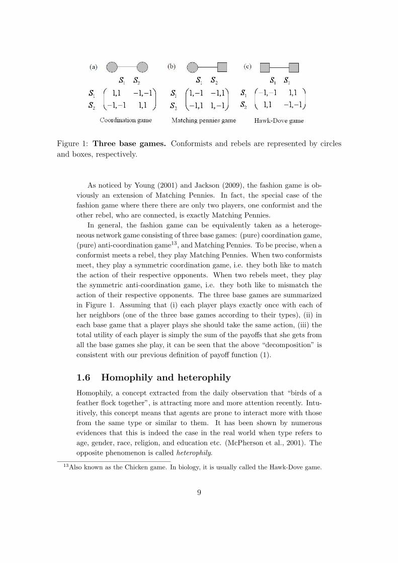
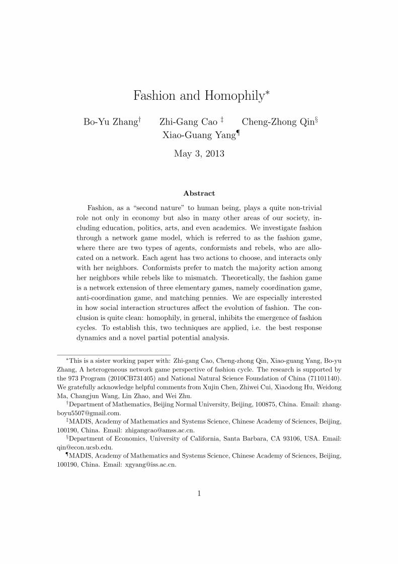
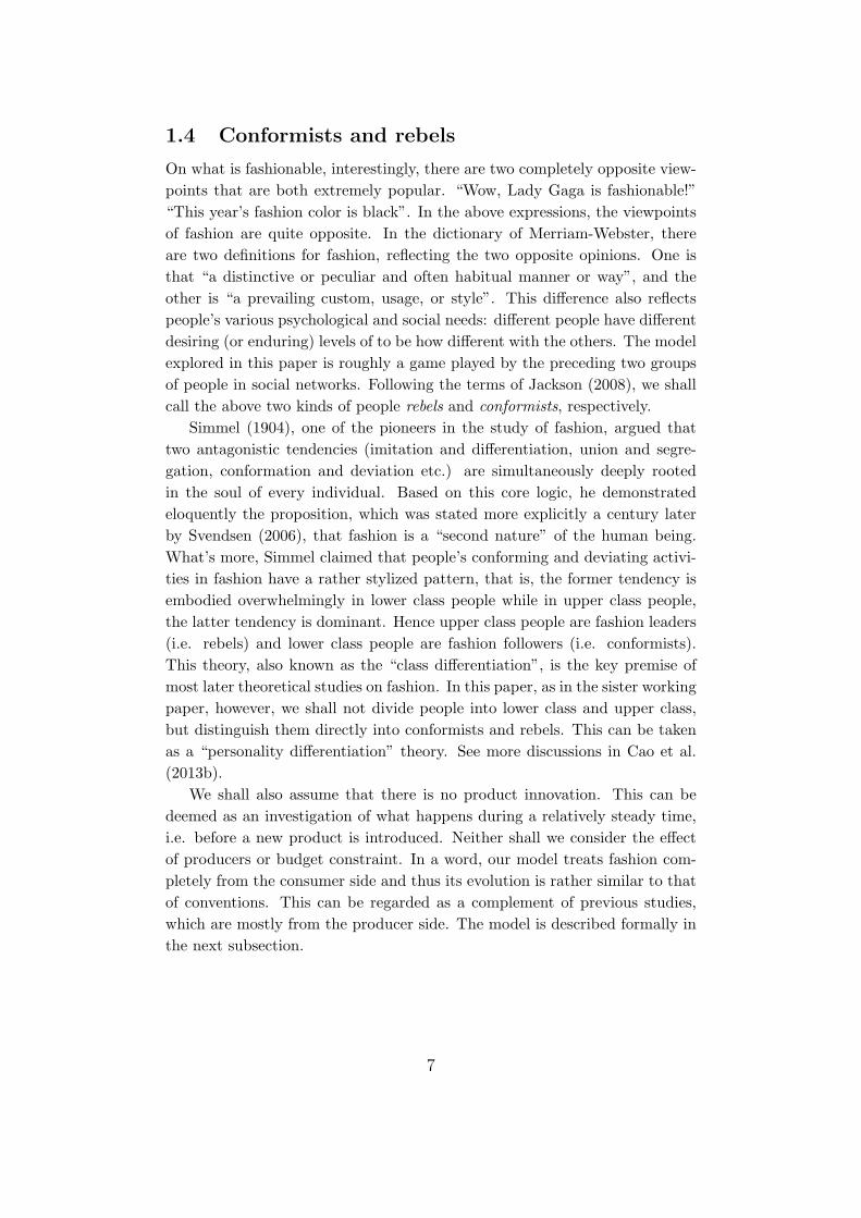
Figure 1: Three base games. Conformists and rebels are represented by circles
and boxes, respectively.
As noticed by Young (2001) and Jackson (2009), the fashion game is ob-viously an extension of Matching Pennies. In fact, the special case of thefashion game where there there are only two players, one conformist and theother rebel, who are connected, is exactly Matching Pennies.
In general, the fashion game can be equivalently taken as a heteroge-neous network game consisting of three base games: (pure) coordination game,(pure) anti-coordination game13, and Matching Pennies. To be precise, when aconformist meets a rebel, they play Matching Pennies. When two conformistsmeet, they play a symmetric coordination game, i.e. they both like to matchthe action of their respective opponents. When two rebels meet, they playthe symmetric anti-coordination game, i.e. they both like to mismatch theaction of their respective opponents. The three base games are summarizedin Figure 1. Assuming that (i) each player plays exactly once with each ofher neighbors (one of the three base games according to their types), (ii) ineach base game that a player plays she should take the same action, (iii) thetotal utility of each player is simply the sum of the payoffs that she gets fromall the base games she play, it can be seen that the above “decomposition” isconsistent with our previous definition of payoff function (1).
1.6 Homophily and heterophily
Homophily, a concept extracted from the daily observation that “birds of afeather flock together”, is attracting more and more attention recently. Intu-itively, this concept means that agents are prone to interact more with thosefrom the same type or similar to them. It has been shown by numerousevidences that this is indeed the case in the real world when type refers toage, gender, race, religion, and education etc. (McPherson et al., 2001). Theopposite phenomenon is called heterophily.
13Also known as the Chicken game. In biology, it is usually called the Hawk-Dove game.
9

The importance of homophily comes not only from its wide existence, butalso from the fact that its existence can have tremendous impacts on people’sbehaviors. For instance, homophily may slow the convergence speed in sociallearning and best-response processes (Golub and Jackson, 2012). It is recentlyshown that homophily can also serve as a similar role as the classical “rich getricher” mechanism in the growth of networks that produces the fundamentalscale-free distribution (Krioukov and Papadopoulos et al., 2012).
An immediate result of homophily, as well as heterophily, is that it mayproduce a social network with some nice patterns. This is understandable,because the long-run relationships that people maintain are usually from fre-quent interactions. In fact, researchers frequently use interactions to replaceor rebuild subject’s various social relationships. After all, social networks arenot directly observable, until the emergence of SNS websites (say Facebookand Twitter). Thus if we look at the final social network, we may find somefeatures measured by certain indices reflecting homophily or heterophily. Ex-ploration of this can be traced back at least to Coleman (1958). See Currariniet. al. (2009) for recent studies.
When there are multiple types of agents on the social network (whereagents are represented by nodes), we should not use the underlying graphalone to denote the structure, but also configuration of agents. Note thatconfiguration here does not mean merely the densities of all types, but alsohow they are distributed. In the fashion game of this paper, even if we knowthat conformists and rebels are half and half, there are still some importantdifferences. Three situations are the easiest to think out: (1) conformists andrebels are distributed evenly, (2) conformists in general have more conformistneighbors and rebels have more rebel ones, (3) conformists tend to have morerelationships with rebels and rebels have more with conformists. The first caseis the well-known mean field case, that has been taken as a key assumption inapproximate analysis of very complicated problems in the field of statisticalphysics and theoretical biology. The second is the essence of homophily andthe third of heterophily. However, when we look at the measuring problemmore carefully, we would find that the above three situations are by no meanscomplete. This will be discussed more detailed in Section 2.
In the fashion game, as we have described in the previous subsection, thereare naturally two types of agents, conformists and rebels, defined throughpeople’s different opinions on what is fashionable. So it is meaningful toinvestigate empirically whether homophily exists in this environment and howit affects the evolution of fashion. The second point is exactly the task of thispaper.
Very interestingly, if we look at the definition of conformists again, wewould find that the behavior of conformists has a very similar essence tothat of homophily. People like to interact more with those of the same type:
10
here “type” can be defined by their actions. The main difference betweenconforming behavior and ordinary homophily is that interaction and type aremixed here: the content of interaction is to choose one’s type. Analogously,the deviating behavior of rebels can be compared with heterophily. Therefore,when homophily and heterophily are considered in the fashion game, it canbe taken that there are double as well as cross homophily and heterophily14.
Recalling the viewpoint of Simmel (1904) that the two opposite tendenciesof conformation and deviation are rooted deeply in our psychology (see alsomore discussions in the sister paper of Cao et al., 2013), we may argue thathomophily and heterophily are also two fundamental tendiencies in a similarsense. Thus we may say that fashion is born associated with homophily andheterophily. What a coincidence!
1.7 Contribution and organization
In the sister working paper, Cao et al. (2013b) argue that heterogeneity ofconsumers, a factor pointed out originally by Simmel (1904), might play animportant role. To be precise, when there is only one type of consumers (eitherconformist or rebels), fashion cycle seems unlikely to occur. This argumentwill be discussed again in this paper (in fact, a slightly more general result isTheorem 3.2).
In this paper, we shall provide a more subtle structural factor, i.e. ho-mophily of the social network, as introduced in the last subsection. Ourmain conclusion is that homophily, in general, is on the negative side of theemergence of fashion cycle (Theorem 3.2, Theorem 4.1). On the other hand,heterophily seems essential to the existence of fashion cycle, and sometimeseven almost sufficient (Theorem 3.1).
Our result is intuitively plausible. Remember that there are three ele-mentary two player games in the fashion game, the coordination game, theanti-coordination game, and the matching pennies game. Pure Nash equilib-rium exists in the former two games but not in the third one. So in order toobserve a “global oscillation”, there should be enough conformist-rebel inter-actions, which naturally corresponds to a network with heterophily.
To establish the main result, the best response dynamics (BRD for short)are applied15 and two approaches are taken: one is rigorous analysis (Section
14This may remind us of the second order partial derivatives in calculus (although may not be soappropriate): ∂2f/∂x2 (mostly conformists with a homophilic network), ∂2f/∂y2 (mostly rebelswith a heterophilic network), ∂2f/∂x∂y (mostly conformists with a heterophilic network), and∂2f/∂y∂x (mostly rebels with a homophilic network).
15In the sister paper of Cao et al. (2013), both simultaneous and non-simultaneous BRDs areconsidered. In this paper, we shall only take into account the non-simultaneous one, i.e. the defaultone when we refer to the concept of BRD.
11

4) and the other approximate analysis (Section 5).In the first approach, our rough logic is to take the empirical proposition
that fashion cycle exists as equivalent to the theoretical one that PNE does notexist. When there is no PNE at all, we cannot expect to have a steady statewhere no agent has incentive to deviate. So as long as the deviating orderis deterministic and fixed, we will definitely observe a cycle, i.e. the stateof the system comes back again after a certain period of time, and that willrepeat again and again16. This is consistent with our intuitive understandingof fashion cycle. However, it should be noted that in fashion cycle, or moreprecisely the limit cycle of the BRD, it is possible that only a small numberof agents deviate at least once but all the others are satisfied all the time andnever deviate at all. That is, fashion cycles might be quite local. What’s more,even if PNE does exist, cycles are still possible, because PNEs may not beobtained by BRD for certain initial action profiles and certain orders (see theexample in Figure 3). So the logic that existence of fashion cycle is identical tothe in-existence of PNE is debatable. Nevertheless, as a theoretical attemptto attack to the complicated phenomenon of fashion, this treatment seems tobe our only, at least first, choice. See the conclusion part of Cao et al. (2013)for more discussions on how to mathematically define fashion cycle.
In the second approach, we transform the stochastic BRD of the fashiongame into a system of ordinary differential equations, and very naturally pe-riodic solutions are taken as fashion cycles. Technically, this transformationrelies crucially on recent developments of the pair approximation and diffusionapproximation skills in the field of theoretical biology (Ohtsuki et al., 2006;Ohtsuki and Nowak, 2006, 2008). This skill, in essence, is a careful imple-mentation of the mean-field method, and has been proved to be very powerfuland at the same time rather reliable.
Organization of the rest paper is as follows. In the next subsection, wegive more related literature. Section 2 is for the measuring of homophily andheterophily. Section 3 gives the preliminary knowledge and some warm-upanalysis. Section 4 and Section 5 are the main parts of this paper, providingthe partial potential analysis and BRD analysis, respectively. Section 7 con-cludes this paper some several discussions. All technical details are postponedto appendices. In particular, Appendix C presents a general framework forthe new technique of partial potential analysis and proves the main result ofSection 4 as an immediate application of it.
16The main reason is that the system is deterministic and the number of possible states is finite.See Cao et al. (2013) for more rigorous description of this logic on simultaneous BRD.
12
1.8 More related literature
Pesendorfer (1995) and Bagwell and Bernheim (1996) are two of the mostinfluential papers studying fashion in the field of economics. The main differ-ences between their models and the fashion game in this paper, as we havementioned, are that consumers are classified into upper class and lower classwhich possess different amount of resources, producers are involved, and noexplicit social network is considered. For fashion games with conformists only,Berninghaus and Schwalbe (1996) showed that simultaneous BRD always con-verges to a cycle of length at most 2. Cannings (2009) noticed that the resultof Berninghaus and Schwalbe holds for fashion games with rebels only too.
Following Young (2001) and Jackson (2008), the exact model of the fash-ion game has recently been seriously studied. Cao and Yang (2011) mainlyconcentrate on the computational side of this model. Through simulation,Cao et. al. (2013b) found that in general people can reach an extraordinarilyhigh level of cooperation via the simple BRD.
The fashion game is also closely related with the “minority game” (Challetand Zhang, 1997; Challet et. al., 2004), an extensively studied model in thefield of social physics. This model, also known as the El Farol Bar problem17,proposed by economist Arthur (1994), is exactly the deviating side of thefashion game. See Cao et al. (2013a, 2013b) for more reviews. It is worthremarking that, in this field, the relation between fashion and their modelis never noticed, and the dominant research method is computer simulationrather than rigorous analysis.
Our research falls also into the booming field of network games (see Goyal,2007; Vega-Redondo, 2007; Jackson, 2008; Jackson and Zenou, 2014). It canbe taken as a new application of this field. What’s more, our model also has itstheoretical interest in this field, namely, it is a mixed model of network gameswith strategic substitutes and network games with strategic complements, thetwo most extensively studied classes of network game models18. In fact, forconformists, it exhibits a simple form of strategic complement, and for rebelsa simple form of strategic substitute works. In a recent model of Hernandezet al. (2013), strategic complements and strategic substitutes can be bothembodied too. However, for a particular setting of parameters, only one effectworks. In our model, except for the two extreme cases, the two effects worksimultaneously.
17El Farol is a bar near Santa Fe, New Mexico.18See e.g. Bramoulle (2007), Bramoulle and Kranton (2007), Hernandez et al. (2013). See also
the review in Jackson (2008), and Jackson and Zenou (2014).
13
2 Measuring Homophily
2.1 More notations
Given a fashion game G = (N, E, T ), we use C(G) to denote the set of con-formists in G, and R(G) the set of rebels. n(G) is the total number of players,c(G) the number of conformists, and r(G) of rebels. That is, c(G) = |C(G)|,r(G) = |R(G)|, n(G) = |N |. Straightforwardly, N = C(G) ∪ R(G) andn(G) = c(G) + r(G). We also use fC to denote the frequency of conformistsin N , i.e.
fC =c(G)n(G)
,
and similarly
fR =r(G)n(G)
is the frequency of rebels in N .Remember that Ni(G) is the set of neighbors of player i in G and ki(G)
her degree. We use
NCi (G) = Ni(G) ∩ C(G) ≡ {ij ∈ E : j ∈ N, Tj = C}
to denote the set of conformist neighbors of player i in G. Similarly,
NRi (G) = Ni(G) ∩R(G) ≡ {ij ∈ E : j ∈ N, Tj = R}
is the set of rebel neighbors of player i in G.For each player i ∈ N , kC
i (G) and kRi (G) are the number of conformist
neighbors and rebel neighbors of i, respectively, i.e.
kCi (G) = |NC
i (G)|,kR
i (G) = |NRi (G)|.
Thus, the total numbers of CC, RR, CR and RC edges in G are respectively
kCC(G) =
∑i∈C(G) kC
i (G)
2,
kRR(G) =
∑i∈R(G) kR
i (G)
2,
kCR(G) =∑
i∈C(G)
kRi (G),
kRC(G) =∑
i∈R(G)
kCi (G).
Since the network is undirected, it is evident that the number of CR edgesequals that of RC ones, i.e.
kCR(G) = kRC(G).
14
2.2 Homophily indices
The following indices measuring homophily levels are very natural, and havebeen widely used in related literature (c.f. Currarini et. al., 2009).
Definition 2.1. Given a fashion game G = (N, E, T ), the homophily indicesof conformists and rebels, denoted by hC and hR, respectively, are defined as
hC =2kCC(G)
2kCC(G) + kCR(G),
hR =2kRR(G)
2kRR(G) + kRC(G).
A prominent advantage of the above definition is that the “macro” mea-sures can be derived naturally from “micro” ones. Given a fashion game G,for any player i,
hi(G) =
{kC
i (G)/ki(G) if i ∈ C
kRi (G)/ki(G) if i ∈ R
(2)
measures the percentage of inner group neighbors of i, and hence is a microlevel of homophily. The relations between the micro and macro measures canbe stated in the following straightforward equations:
hC =∑
i∈C ki(G)hi(G)∑i∈C ki(G)
,
hR =∑
i∈R ki(G)hi(G)∑i∈R ki(G)
.
The above relations tell us that the conformist homophily level of G isexactly the weighted average of the homophily levels of all the conformists,where the weights are their degrees. And so is the rebel homophily level of G.
2.3 Conformist (rebel) relative homophily
When we talk about whether a fashion game satisfies homophily or not w.r.t.a particular kind of players, we can simply compare the corresponding ho-mophily index with its relative fraction. The definition below is standard (c.f.Currarini et. al., 2009).
Definition 2.2. Suppose G is a fashion game. We say that G satisfies con-formist (rebel) relative homophily if hC > fC (hR > fR). On the other hand,we say that G satisfies conformist (rebel) relative heterophily if hC < fC
(hR < fR). The left case, hC = fC (hR = fR), is called conformist (rebel)baseline homophily.
15
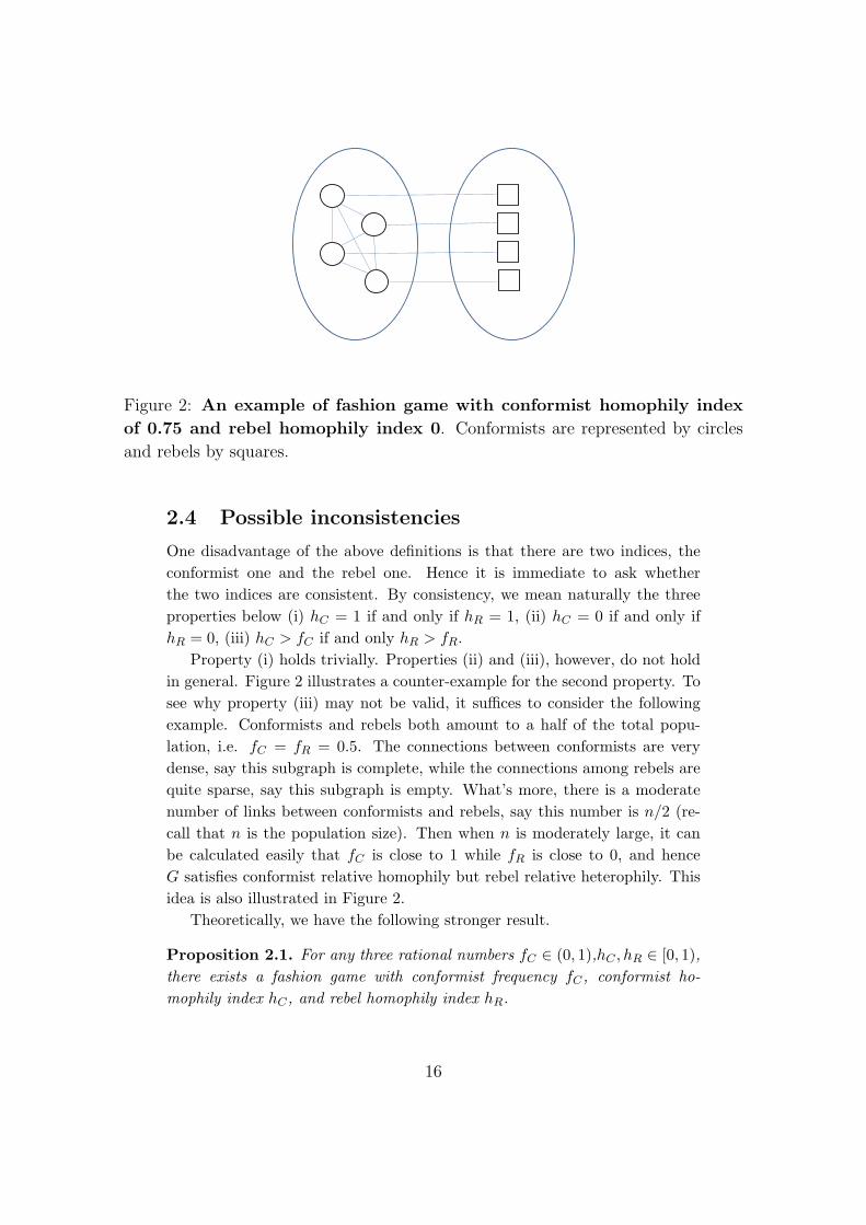
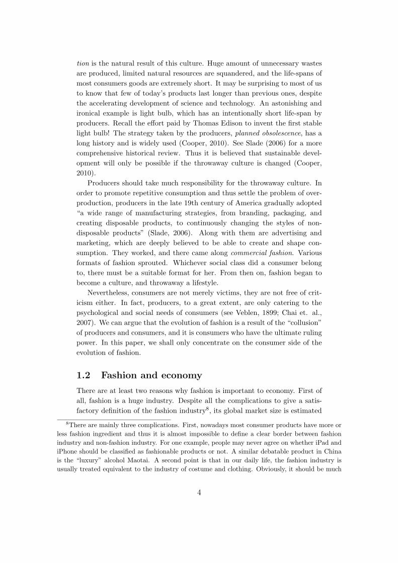
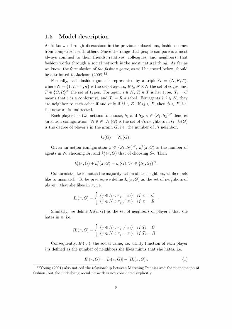
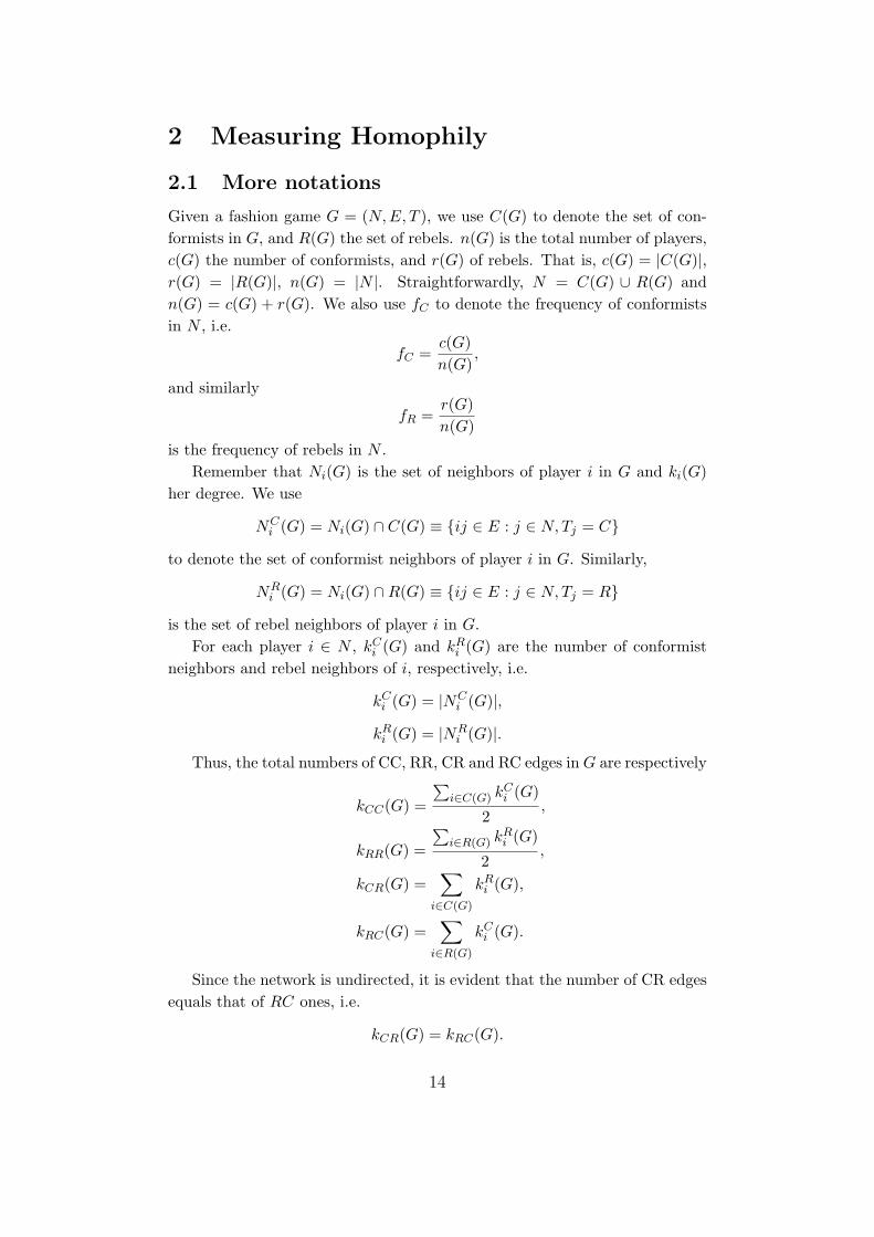
Figure 2: An example of fashion game with conformist homophily index
of 0.75 and rebel homophily index 0. Conformists are represented by circles
and rebels by squares.
2.4 Possible inconsistencies
One disadvantage of the above definitions is that there are two indices, theconformist one and the rebel one. Hence it is immediate to ask whetherthe two indices are consistent. By consistency, we mean naturally the threeproperties below (i) hC = 1 if and only if hR = 1, (ii) hC = 0 if and only ifhR = 0, (iii) hC > fC if and only hR > fR.
Property (i) holds trivially. Properties (ii) and (iii), however, do not holdin general. Figure 2 illustrates a counter-example for the second property. Tosee why property (iii) may not be valid, it suffices to consider the followingexample. Conformists and rebels both amount to a half of the total popu-lation, i.e. fC = fR = 0.5. The connections between conformists are verydense, say this subgraph is complete, while the connections among rebels arequite sparse, say this subgraph is empty. What’s more, there is a moderatenumber of links between conformists and rebels, say this number is n/2 (re-call that n is the population size). Then when n is moderately large, it canbe calculated easily that fC is close to 1 while fR is close to 0, and henceG satisfies conformist relative homophily but rebel relative heterophily. Thisidea is also illustrated in Figure 2.
Theoretically, we have the following stronger result.
Proposition 2.1. For any three rational numbers fC ∈ (0, 1),hC , hR ∈ [0, 1),there exists a fashion game with conformist frequency fC , conformist ho-mophily index hC , and rebel homophily index hR.
16
2.5 Relative homophily/heterophily
According to Proposition 2.1, we can say that the three parameters, fC , hC ,and hR, are independent of each other. So when we say a fashion game satisfiesrelative homophily (heterophily), it is safe to require that this is true for bothtypes.
Definition 2.3. A fashion game is called relatively homophilic/heterophilicwhen it satisfies both conformist relative homophily/heterophily and rebel ho-mophily/heterophily.
2.6 Homophily/heterophily on average
The homophily concept defined in the last subsection is usually too restrictive,and we find that a relaxed one is useful. Before presenting the definition, weneed to define the average homophily index for the fashion game.
Definition 2.4. Given a fashion game G, its average homophily index, de-noted by h(G), is defined as the average of its conformist homophily index andthe rebel one , i.e.
h(G) =hC + hR
2.
The following definition is natural.
Definition 2.5. We say that a fashion game G satisfies homophily on averageif h(G) > 1/2 and heterophily on average if h(G) < 1/2.
It turns out that homophily on average and heterophily on average areequivalent to certain very nice properties of inner group and cross group edgefrequencies.
Proposition 2.2. A fashion game G is homophilic on average if and only ifthe frequency of CR edges is less than one half, i.e.,
kCR(G) < kCC(G) + kRR(G).
2.7 Complete homophily/heterophily
The following natural concepts are also useful.
Definition 2.6. We say that a fashion game G satisfies complete homophilyif h(G) = 0 and complete heterophily if h(G) = 1.
17
In general, it is difficult to estimate the frequency of edges if we only knowthe average homophily level. However, when G satisfies complete homophily,it must be true that kCR(G) = kRC(G) = 0. That is, no conformist has anyconnection (direct or indirect) with a rebel, and vice versa. And when G
satisfies complete heterophily, we must have kCC(G) = kRR(G) = 0. That is,no conformist has any conformist neighbor, and no rebel has any rebel one19.
2.8 Relations between the three homophilies
The proposition below is evident.
Proposition 2.3. If there are both conformists and rebels in a fashion game,i.e. 0 < fC < 1, then complete homophily (heterophily) implies relative ho-mophily (heterophily), which is further stronger than homophily (heterophily)on average.
2.9 Regular graphs
For regular graphs, which are defined as those that all nodes have identicaldegrees, we have the following nice property.
Proposition 2.4. Suppose G is a fashion game. If the underlying graph isregular, then the three concepts, conformist relative homophily, rebel relativehomophily and homophily on average, are identical.
Thanks to the above proposition, it is definite that a fashion game witha regular underlying graph satisfies either relative homophily, or relative het-erophily, or baseline homophily.
3 Potential Analysis
Like Matching Pennies, the fashion game has an obvious mixed Nash equilib-rium: each player plays half S1 and half S2. It can be checked that this is infact the only mixed Nash equilibrium.
In this paper, we are more interested in pure strategy Nash equilibria(PNE for short). A (pure) strategy profile π∗ ∈ {S1, S2}N is a PNE if playershave no incentive to change their actions. Since Ei(0, π−i) + Ei(1, π−i) = 0for all π−i ∈ {S1, S2}N\{i}, we can see that π∗ is a PNE if and only if
Ei(π∗) ≥ 0,∀i ∈ N.
19Using the terminology of graph theory, this means that the underlying graph is bipartite, withone side of all conformists and the other side of all rebels.
18

Proposition 3.1. The fashion game must have an even number of PNEs.
Proof to the above proposition is straightforward, because it is an immedi-ate result of our payoff settings that the two actions S1 and S2 are symmetric.In fact, if π∗ is a PNE, then π∗ must also be a PNE, where π∗i is a differentaction with π∗i for all i ∈ N . The above proposition embodies the essenceof fashion as symbolic consumption. To be precise, what a single player con-sumes does not matter, what matters is the comparison with her neighbors.Therefore, if all people switch their actions, nothing essential is changed.
3.1 The complete heterophily case
Existence of PNE, in general, cannot be guaranteed. For instance, pairingone conformist and one rebel in a dyad results in no PNE, as in the game ofMatching Pennies. If we require the network to be connected, things cannotbe improved at all. Below is a more general negative result.
Theorem 3.1. Let G be a fashion game. If h(G) = 0 i.e. the underlyingnetwork is completely heterophily, and at least one agent has an odd degree,then G does not possess any PNE.
Note that in the above proposition, the second condition (oddness of atleast one player) is quite weak. Therefore, for almost all networks, the con-dition for the above proposition is equivalent to an requirement of completeheterophily. To put it another way, complete heterophily implies almost al-ways the inexistence of an PNE20.
3.2 The complete homophily case
It is natural to ask the other polar case, i.e complete homophily. We arehappy to see that this case always possess an PNE.
Theorem 3.2. Let G be a fashion game. If h(G) = 1, i.e. the underlyingnetwork satisfies complete homophily, then G is an exact potential game, andthus possesses at least one PNE.
This result is implied by a more general result of Blume (1993), whichstates that symmetric social interaction games possess an exact potential func-tion (see also Bramoulle, 2007). In fact, h(G) = 1 says that no inter-groupconnections exist between conformists and rebels and hence all interactions
20It is shown by Cao and Yang (2011) that if the underlying graph is a line, then completeheterophily is the only case that PNE does not exist. For rings (where no player has an odddegree), complete heterophily is a necessary but not sufficient condition for the in-existence ofPNE.
19

are symmetric. As a corollary, network coordination games and network anti-coordination games, which are two special fashion games satisfying completehomophily, are both exact potential games21.
Since the rigorous proof to the above theorem is not hard (the potentialfunction can be defined as a half of the total utilities of all players), we presentit in Appendix B.1 for the convenience of the reader.
4 Partial Potential Analysis
Standard theory of potential games tells us not only that PNE is guaranteedfor the completely homophilic fashion game, but also that, from any initialaction profile, PNE can be reached through the simple best (in fact better)response dynamics. And this is true for an arbitrary deviating order. Thepotential argument fails to work for the case that PNE exists but might notbe reached through best response dynamics (see the example in Figure 3).We shall investigate this case in this section.
4.1 Main idea
This is done through a partial potential analysis. The basic idea of this argu-ment is as follows. We let a part of players fix their actions and let the leftones deviate whenever unsatisfied (one deviation per step). However, if wecan find an “arrow” for this process (i.e. a partial potential function, which isbounded), and thus it cannot continue forever, then we will definitely arriveat a pure action profile where all the “free” players are satisfied. The largerthe free set is, the better the final action profile will be. What’s more, if wecan choose a partial action profile for the fixed ones such that they are alwayssatisfied whatever the free ones choose, then we will arrive at a PNE.
4.2 Strong homophilies
To present our main result, the following two definitions are needed.
Definition 4.1 (Strong Conformist Homophily). Let G be a fashion game.If each conformist has no less conformist neighbors than rebels ones, i.e.
hi(G) ≥ 0.5,∀i ∈ C,
then we say that G satisfies strong conformist homophily.
21Very interestingly, a PNEs in the network (pure) anti-coordination game corresponds to anunfriendly partition, a concept that has been studied by graph theorists (Aharoni et. al., 1990), ofthe underlying graph.
20

Definition 4.2 (Strong Rebel Homophily). Let G be a fashion game. If thereexists a partition of the rebel set R, {R1, R2}, such that
|Ni(G) ∩R2| ≥ 0.5|Ni(G)|,∀i ∈ R1,
|Nj(G) ∩R1| ≥ 0.5|Nj(G)|,∀j ∈ R2,
then we say that G satisfies strong rebel homophily.
The proposition below shows that the two homophilies are weaker thancomplete homophily but almost always stronger than homophily on average.
Proposition 4.1. Let G be a fashion game.(a) If G possesses complete homophily, i.e. h(G) = 1, then it satisfies both
strong conformist homophily and strong rebel homophily.(b) If G satisfies both strong conformist homophily and strong rebel ho-
mophily, then h(G) ≥ 0.5.
Proof. (a) Strong conformist homophily is obvious because h(G) = 1 impliesthat hi(G) = 1 for all players. To show that strong rebel homophily is alsotrue, let aN be an arbitrary PNE of G. Due to Theorem 3.2, aN exists. Wedefine R1 as the set of rebels that choose S1 in aN , and R2 the set of rebelschoosing S2 in aN . aN is a PNE tells us that all the rebels are satisfied in aN ,i.e. each player i ∈ R has at least a half of her neighbors she likes. Note thath(G) = 1 means rebels only have rebel neighbors, so strong rebel homophilyholds.
(b) If a fashion game satisfies strong conformist homophily, then hC ≥ 0.5since hC is a convex combination for all the hi(G), i ∈ C. Similarly, sincefor any strong rebel homophily fashion game G, it holds for all i ∈ R thathi(G) ≥ 0.5, it must be true that hR ≥ 0.5. Thus, hC + hR ≥ 1.
4.3 Main result
Jackson (2008) observed that when (i) all conformists have a homophily indexof at least 0.5 and (ii) all rebels have a homophily index of at most 0.5, thenPNE exists. In fact, it can be checked that all conformists choose S1 and allrebels choose S2 is a PNE.
The conditions used by Jackson are stronger than strong conformist ho-mophily. To be precise, the first part of his condition is exactly strong con-formist homophily. Half of the following theorem is an improvement of Jack-son’s result, showing that the condition that rebels should have an uppderbound of 0.5 on their homphily index is actually redundant.
Theorem 4.1. Let G be a fashion game. If G satisfies either strong con-formist homophily or strong rebel homophily, then PNE exists.
21
As to PNE existence, the above theorem is also stronger than Theorem 3.1,because h(G) = 1 implies both conformist homophily and rebel homophily,as shown in Proposition 4.1. However, Theorem 3.1 still has its right to exist,because it tells more: the complete homophily case of the fashion game is anexact potential game, which is not implied in Theorem 4.1.
Correctness of Theorem 4.1 follows naturally from the general frameworkof partial potential analysis introduced in Appendix C. The rough idea behindthat proof has already been sketched in Subsection 4.1. To be more specific,when the fashion game G satisfies strong conformist homophily, then we canlet all the conformist choose S1, then they are always satisfied whatever therebel choose, because each of them has already at least a half of their neighborstake the same action as they do. Then we let the rebels take arbitrary initialactions and deviate in an arbitrary order whenever unsatisfied. Just as wehave shown that the fashion game with all rebels is a potential game, theabove reduced game (with all conformists choosing S1) can also shown to be apotential game. In fact, this is exactly the definition of partial potential game,i.e. a strategic game where there exists a subset of players and a partial actionprofile for these players such that the corresponding reduced game (where theplayer set is the original player set minus the previous subset of players) is apotential game. Using this property, we know that the deviating process ofrebels will eventually stop at a state where all the rebels are satisfied. Sinceall the conformists are satisfied too, we actually arrive at a PNE. The proof tothe second part of Theorem 4.1 is analogous, and the only point that shouldbe noticed is that when a fashion game G satisfies strong rebel homophily,with the rebel partition {R1, R2} as in the definition, we can let rebels in R1
choose S1 and rebels in R2 choose S2, then all the rebels are always satisfiedwhatever the conformists choose.
4.4 An example
In general, fashion game is not an exact potential game in neither of thethe two cases in Theorem 4.1. In fact, using Corollary 2.9 of Monderer andShapley (1996), it can be checked that the fashion game is definitely not anexact potential game when there is at least one conformist-rebel edge in theunderlying graph.
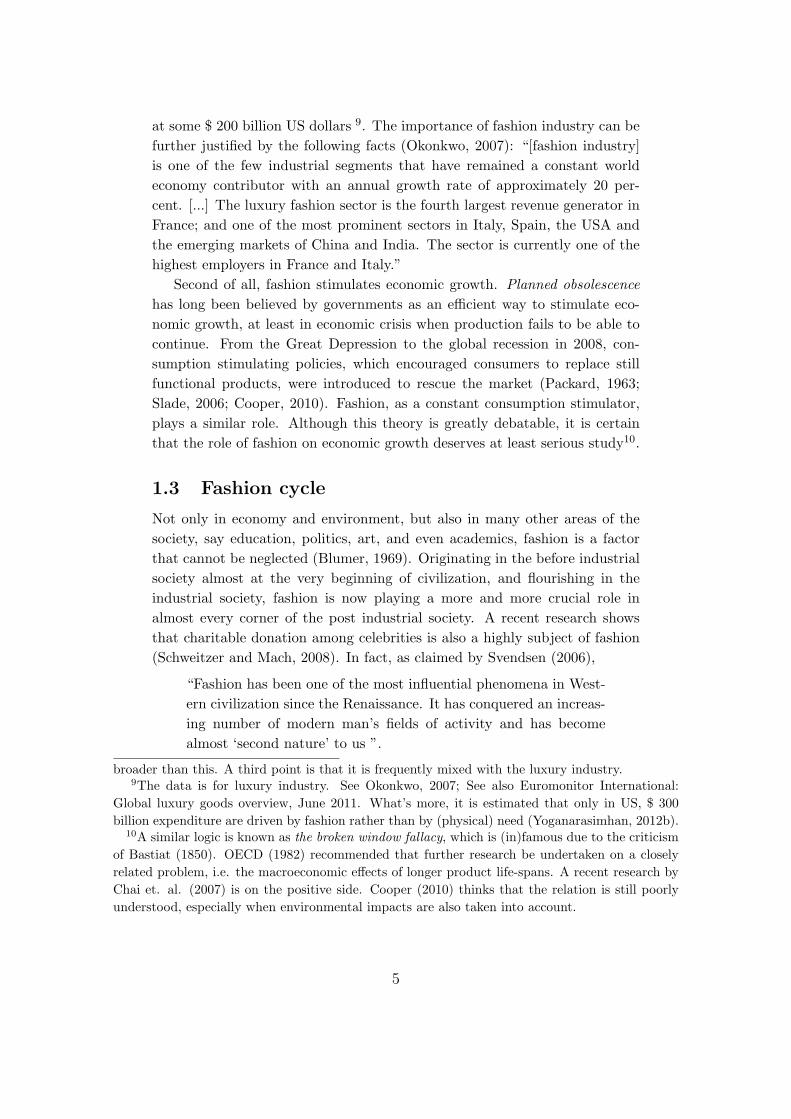
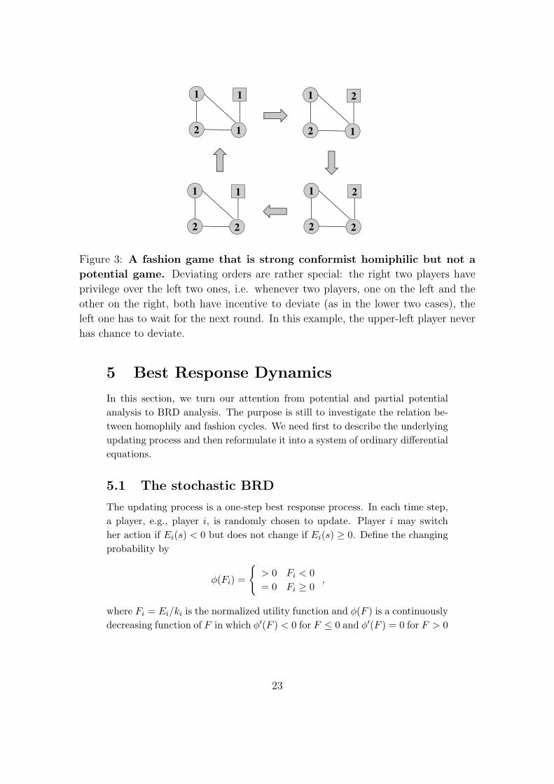
What’s more, as shown in Figure 3, fashion games satisfying conditionsin Theorem 4.1 may not even be ordinary potential games. However, theyare both exact partial potential games (Theorem C.2 in Appendix C.3). Thismeans that our concept is a substantial extension of the original one, and thusit can be used to prove PNE existence for non-potential games.
22
1 1
2 1
2 1
2 1
2 1
2 2
1 1
2 2
Figure 3: A fashion game that is strong conformist homiphilic but not a
potential game. Deviating orders are rather special: the right two players have
privilege over the left two ones, i.e. whenever two players, one on the left and the
other on the right, both have incentive to deviate (as in the lower two cases), the
left one has to wait for the next round. In this example, the upper-left player never
has chance to deviate.
5 Best Response Dynamics
In this section, we turn our attention from potential and partial potentialanalysis to BRD analysis. The purpose is still to investigate the relation be-tween homophily and fashion cycles. We need first to describe the underlyingupdating process and then reformulate it into a system of ordinary differentialequations.
5.1 The stochastic BRD
The updating process is a one-step best response process. In each time step,a player, e.g., player i, is randomly chosen to update. Player i may switchher action if Ei(s) < 0 but does not change if Ei(s) ≥ 0. Define the changingprobability by
φ(Fi) =
{> 0 Fi < 0= 0 Fi ≥ 0
,
where Fi = Ei/ki is the normalized utility function and φ(F ) is a continuouslydecreasing function of F in which φ′(F ) < 0 for F ≤ 0 and φ′(F ) = 0 for F > 0
23
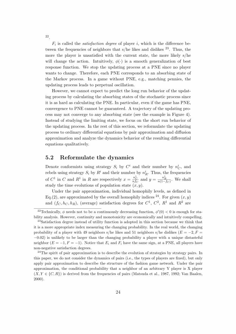
22.Fi is called the satisfaction degree of player i, which is the difference be-
tween the frequencies of neighbors that s/he likes and dislikes 23. Thus, themore the player is unsatisfied with the current state, the more likely s/hewill change the action. Intuitively, φ(·) is a smooth generalization of bestresponse function. We stop the updating process at a PNE since no playerwants to change. Therefore, each PNE corresponds to an absorbing state ofthe Markov process. In a game without PNE, e.g., matching pennies, theupdating process leads to perpetual oscillation.
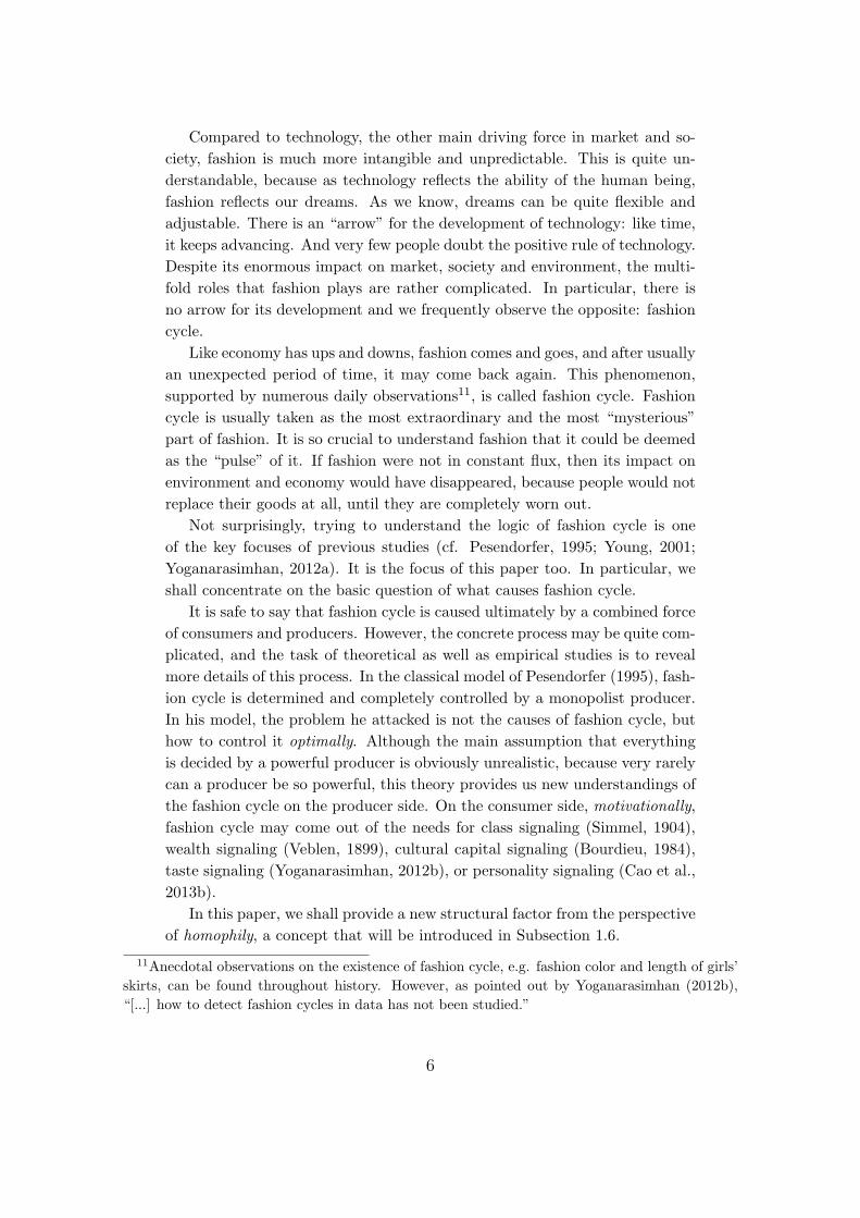
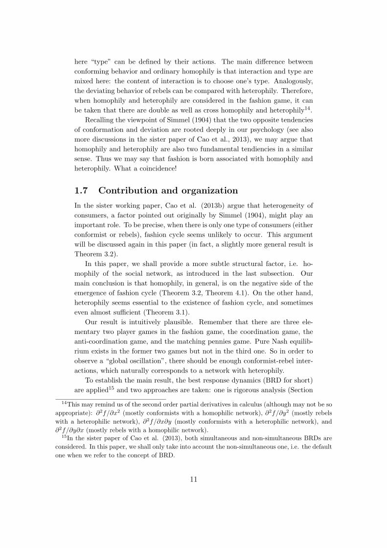
However, we cannot expect to predict the long run behavior of the updat-ing process by calculating the absorbing states of the stochastic process sinceit is as hard as calculating the PNE. In particular, even if the game has PNE,convergence to PNE cannot be guaranteed. A trajectory of the updating pro-cess may not converge to any absorbing state (see the example in Figure 4).Instead of studying the limiting state, we focus on the short run behavior ofthe updating process. In the rest of this section, we reformulate the updatingprocess to ordinary differential equations by pair approximation and diffusionapproximation and analyze the dynamics behavior of the resulting differentialequations qualitatively.
5.2 Reformulate the dynamics
Denote conformists using strategy Si by Ci and their number by niC , and
rebels using strategy Si by Ri and their number by niR. Thus, the frequencies
of C1 in C and R1 in R are respectively x = n1C
nfCand y = n1
Rn(1−fC) . We shall
study the time evolutions of population state (x, y).Under the pair approximation, individual homophily levels, as defined in
Eq.(2), are approximated by the overall homophily indices 24. For given (x, y)and (fC , hC , hR), (average) satisfaction degrees for C1, C2, R1 and R2 are
22Technically, φ needs not to be a continuously decreasing function, φ′(0) < 0 is enough for sta-bility analysis. However, continuity and monotonicity are economically and intuitively compelling.
23Satisfaction degree instead of utility function is adopted in this section because we think thatit is a more appropriate index measuring the changing probability. In the real world, the changingprobability of a player with 49 neighbors s/he likes and 51 neighbors s/he dislikes (E = −2, F =−0.02) is unlikely to be larger than the changing probability a player with a unique distastefulneighbor (E = −1, F = −1). Notice that Ei and Fi have the same sign, at a PNE, all players havenon-negative satisfaction degrees.
24The spirit of pair approximation is to describe the evolution of strategies by strategy pairs. Inthis paper, we do not consider the dynamics of pairs (i.e., the types of players are fixed), but onlyapply pair approximation to describe the structure of the fashion game network. Under the pairapproximation, the conditional probability that a neighbor of an arbitrary Y player is X player(X, Y ∈ {C, R}) is derived from the frequencies of pairs (Matsuda et al., 1987, 1992; Van Baalen,2000).
24
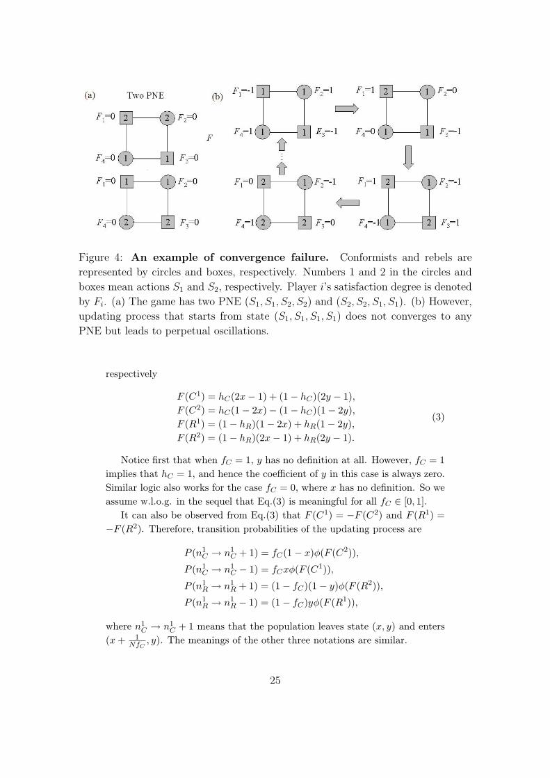
Figure 4: An example of convergence failure. Conformists and rebels are
represented by circles and boxes, respectively. Numbers 1 and 2 in the circles and
boxes mean actions S1 and S2, respectively. Player i’s satisfaction degree is denoted
by Fi. (a) The game has two PNE (S1, S1, S2, S2) and (S2, S2, S1, S1). (b) However,
updating process that starts from state (S1, S1, S1, S1) does not converges to any
PNE but leads to perpetual oscillations.
respectively
F (C1) = hC(2x− 1) + (1− hC)(2y − 1),F (C2) = hC(1− 2x)− (1− hC)(1− 2y),F (R1) = (1− hR)(1− 2x) + hR(1− 2y),F (R2) = (1− hR)(2x− 1) + hR(2y − 1).
(3)
Notice first that when fC = 1, y has no definition at all. However, fC = 1implies that hC = 1, and hence the coefficient of y in this case is always zero.Similar logic also works for the case fC = 0, where x has no definition. So weassume w.l.o.g. in the sequel that Eq.(3) is meaningful for all fC ∈ [0, 1].
It can also be observed from Eq.(3) that F (C1) = −F (C2) and F (R1) =−F (R2). Therefore, transition probabilities of the updating process are
P (n1C → n1
C + 1) = fC(1− x)φ(F (C2)),
P (n1C → n1
C − 1) = fCxφ(F (C1)),
P (n1R → n1
R + 1) = (1− fC)(1− y)φ(F (R2)),
P (n1R → n1
R − 1) = (1− fC)yφ(F (R1)),
where n1C → n1
C + 1 means that the population leaves state (x, y) and enters(x + 1
NfC, y). The meanings of the other three notations are similar.
25
Applying the diffusion approximation (Traulsen et al., 2005, 2006), theabove process could be described by the stochastic replicator-mutator equa-tions
{dxdt = (1− x)φ(F (C2))− xφ(F (C1)) +
∑3i=1 c1i(x, y)ξi(t)
dydt = (1− y)φ(F (R2))− yφ(F (R1)) +
∑3i=1 c3i(x, y)ξi(t)
, (4)
where c1i(x, y) and c3i(x, y) are diffusion terms, and ξ1(t) and ξ3(t) are un-correlated Gaussian white noise with unit variance (see details in AppendixD.1).
For finite populations, the diffusion terms vanish at a rate of 1√n
as n →∞ and the evolutions of x and y could be approximated by the followingdeterministic dynamics (Traulsen et al, 2005; Ohtsuki and Nowak, 2006):
{dxdt = (1− x)φ(F (C2))− xφ(F (C1))dydt = (1− y)φ(F (R2))− yφ(F (R1))
. (5)
It is interesting to notice that Eq.(5) is independent of fC , and only decidedby the homophily indices hC and hR, because this is true for Eq.(3)25.
Before proceeding to the analysis of Eq.(5), we provide some simple yetuseful observations.
Observation 1. The following statements for φ(F (C1)) and φ(F (C2)) aretrue.
(a) At least one of φ(F (C1)) and φ(F (C2)) is zero;(b) φ(F (C1)) = φ(F (C2)) = 0 if and only if hCx + (1− hC)y = 1/2.
Proof to the above observations is trivial. The reader only needs to re-call the definition of φ(·) and notice the relation of F (C1) = −F (C2). Theobservations below are analogous.
Observation 2. Suppose fC ∈ (0, 1), then the following statements for φ(F (R1))and φ(F (R2)) are true.
(a) At least one of φ(F (R1)) and φ(F (R2)) is zero;(b) φ(F (R1)) = φ(F (R2)) = 0 if and only if (1− hR)x + hRy = 1/2.
5.3 Benchmark cases
If the population consists entirely of conformists, i.e. fC = 1, then the fashiongame is equivalent to the well known coordination game, and Eq.(5) boils downto
dx
dt= (1− x)φ(F (C2))− xφ(F (C1)). (6)
25Recall that fC is almost surely independent of hC and hR (Proposition 2.1).
26
Notice again that fC = 1 implies hC = 1, so we have
F (C1) = −F (C2) = 2x− 1. (7)
Let’s calculate the fixed points of Eq.(6). Suppose now x is an interior fixedpoint, i.e. x /∈ {0, 1}. Then Observation 1(a) tells us that it must be the casethat both F (C1) and F (C2) are zero, because otherwise (1 − x)φ(F (C2)) −xφ(F (C1)) cannot be zero. From Eq.(7) we get immediately that x = 1/2.Notice also that dx
dt > 0 when x > 1/2 and dxdt < 0 when x < 1/2, hence 1/2
is unstable. It can be easily checked that x = 0 and x = 1 are both boundaryfixed points, and they are locally asymptotically stable. Below is a summaryof the above analysis.
Proposition 5.1. Eq.(6) has three fixed points, x = 0, x = 1 and x = 1/2.The two boundary fixed points are locally asymptotically stable and the interiorone is unstable.
In contrast, if the population consists of homogenous rebels, i.e. fC = 0,the fashion game is equivalent to the Hawk-Dove game and Eq.(5) becomes
dy
dt= (1− y)φ(F (R2))− yφ(F (R1)). (8)
In this case we have F (R1) = −F (R2) = 1−2y. And 1/2 is still an interiorfixed point. The difference is that it becomes globally stable, because dy
dt < 0when y > 1/2 and dy
dt > 0 when y < 1/2. Also, it can be checked that neither0 nor 1 is a fixed point in this case. To put it formally, we have the followingproposition.
Proposition 5.2. Eq. (8) has a unique fixed point, y = 1/2, which is globallystable.
5.4 The general case
From Observations 1 and 2, we know that (x, y) ∈ [0, 1]2 is a fixed point ofEq.(5) if and only if
xφ(F (C1)) = (1− x)φ(F (C2)) = yφ(F (R1)) = (1− y)φ(F (R2)) = 0. (9)
We first calculate the interior fixed point (x, y) ∈ (0, 1)2, which, due toEq.(9), must satisfy
φ(F (C2)) = φ(F (C1)) = φ(F (R2)) = φ(F (R1)) = 0.
Using Observation 1(b) and Observation 2(b), we get{
hCx + (1− hC)y = 1/2(1− hR)x + hRy = 1/2
. (10)
27
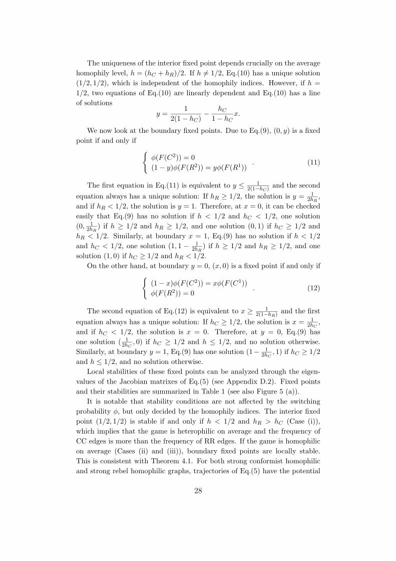
The uniqueness of the interior fixed point depends crucially on the averagehomophily level, h = (hC + hR)/2. If h 6= 1/2, Eq.(10) has a unique solution(1/2, 1/2), which is independent of the homophily indices. However, if h =1/2, two equations of Eq.(10) are linearly dependent and Eq.(10) has a lineof solutions
y =1
2(1− hC)− hC
1− hCx.
We now look at the boundary fixed points. Due to Eq.(9), (0, y) is a fixedpoint if and only if
{φ(F (C2)) = 0(1− y)φ(F (R2)) = yφ(F (R1))
. (11)
The first equation in Eq.(11) is equivalent to y ≤ 12(1−hC) and the second
equation always has a unique solution: If hR ≥ 1/2, the solution is y = 12hR
,and if hR < 1/2, the solution is y = 1. Therefore, at x = 0, it can be checkedeasily that Eq.(9) has no solution if h < 1/2 and hC < 1/2, one solution(0, 1
2hR) if h ≥ 1/2 and hR ≥ 1/2, and one solution (0, 1) if hC ≥ 1/2 and
hR < 1/2. Similarly, at boundary x = 1, Eq.(9) has no solution if h < 1/2and hC < 1/2, one solution (1, 1 − 1
2hR) if h ≥ 1/2 and hR ≥ 1/2, and one
solution (1, 0) if hC ≥ 1/2 and hR < 1/2.On the other hand, at boundary y = 0, (x, 0) is a fixed point if and only if
{(1− x)φ(F (C2)) = xφ(F (C1))φ(F (R2)) = 0
. (12)
The second equation of Eq.(12) is equivalent to x ≥ 12(1−hR) and the first
equation always has a unique solution: If hC ≥ 1/2, the solution is x = 12hC
,and if hC < 1/2, the solution is x = 0. Therefore, at y = 0, Eq.(9) hasone solution ( 1
2hC, 0) if hC ≥ 1/2 and h ≤ 1/2, and no solution otherwise.
Similarly, at boundary y = 1, Eq.(9) has one solution (1− 12hC
, 1) if hC ≥ 1/2and h ≤ 1/2, and no solution otherwise.
Local stabilities of these fixed points can be analyzed through the eigen-values of the Jacobian matrixes of Eq.(5) (see Appendix D.2). Fixed pointsand their stabilities are summarized in Table 1 (see also Figure 5 (a)).
It is notable that stability conditions are not affected by the switchingprobability φ, but only decided by the homophily indices. The interior fixedpoint (1/2, 1/2) is stable if and only if h < 1/2 and hR > hC (Case (i)),which implies that the game is heterophilic on average and the frequency ofCC edges is more than the frequency of RR edges. If the game is homophilicon average (Cases (ii) and (iii)), boundary fixed points are locally stable.This is consistent with Theorem 4.1. For both strong conformist homophilicand strong rebel homophilic graphs, trajectories of Eq.(5) have the potential
28

Parameters Fixed points Stability conditions(i) h < 1/2, hC < 1/2 (1/2, 1/2) hR − hC > 0
(ii) h > 1/2, hR ≥ 1/2(1/2, 1/2) unstable
(0, 12hR
), (1, 1− 12hR
) stable
(iii) h > 1/2, hC > 1/2, hR < 1/2(1/2, 1/2) unstable
(0, 1), (1, 0) stable
(iv) h < 1/2, hC > 1/2, hR < 1/2(1/2, 1/2) unstable
(0, 1), (1, 0) stable( 12hC
, 0), (1− 12hC
, 1) unstable
(v) hC = 1/2, hR < 1/2(1/2, 1/2) unstable
(0, 1), (1, 0) unstable(vi) h = 1/2 y = 1
2(1−hC) − hC1−hC
x neutral stable
Table 1: Fixed points of Eq.(5) and their stabilities.
converging to boundary fixed points in which all conformists take the sameaction but different rebels may adopt different actions.
Interestingly, the global dynamic behavior of Eq.(5) is also affected littleby the switching probability φ. In particular, the emergence of fashion cycledepends only on homophily indices.
Theorem 5.1. Fashion cycle, i.e. periodic solution of Eq.(5), emerges only ifthe fashion game is heterophilic on average. In contrast, if the fashion game ishomophilic on average, almost all trajectories of Eq.(5) converge to boundaryfixed points.
The only exception in the second part of the above theorem is the tra-jectory with initial value (1/2, 1/2) since (1/2, 1/2) is always a fixed point ofEq.(5). See the proof in Appendix D.3.
Furthermore, the following property of fashion cycle can be obtained byanalyzing the zero-isoclines of Eq.(5) (see Appendix D.3 for detail).
Proposition 5.3. If fashion cycle exists, the rotation of fashion cycle mustbe clockwise, i.e., conformists change their actions following the changes ofrebels.
The above proposition shows that the behaviors of rebels and conformistsare consistent with their name. In a fashion cycle, starting from the situationthat the majority of people using the same action, rebels first begin to switchto the unpopular action since they want to be distinctive. However, whenconformists realized that the action of their (rebel) neighbors are differentfrom them, they will change accordingly which will lead again to the casethat most of players are in the same action (see Figure 7).
29

Parameters Fixed points Stability conditions
(i) hC < fC , hC < 1/2 (1/2, 1/2) fC < 1/2
(ii) hC > fC , hR ≥ 1/2(1/2, 1/2) unstable
(0, 12hR
), (1, 1− 12hR
) stable
(iii) hC > fC , hR < 1/2(1/2, 1/2) unstable
(0, 1), (1, 0) stable
(iv) hC < fC , hC > 1/2
(1/2, 1/2) unstable
(0, 1), (1, 0) stable
( 12hC
, 0), (1− 12hC
, 1) unstable
(v) hC < fC , hC = 1/2(1/2, 1/2) unstable
(0, 1), (1, 0) unstable
(vi) hC = fC y = 12(1−hC)
− hC
1−hCx neutral stable
Table 2: Fixed points of Eq.(5) and their stabilities in regular graphs.
For regular graphs, homophily on average (i.e., h > 1/2) implies that thefashion game is relative homophilic (i.e., hC > fC and hR > fR). Therefore, aclear connection between the stabilities of fixed points and relative homophilycan be established. (see Table 2 and Figure 5 (b))
Theorem 5.2. For regular graphs, fashion cycle, i.e. periodic solution ofEq.(5), emerges only if the fashion game is heterophilic. In contrast, in ahomophilic game, almost all trajectories of Eq.(5) converge to boundary fixedpoints.
Here we provide an intuition how the global dynamic behavior of Eq. (5)is affected by the frequencies of edges. Propositions 5.1 and 5.2 indicate thatthe interior fixed point is unstable if the game consists of CC edges (e.g.,coordination game) and is globally stable if the game consists of RR edges(e.g., Hawk-Dove game). Intuitively, RR edges push the trajectories of Eq.(5)to the interior fixed point but CC edges drive them away. On the other hand,if the game consists of CR edges (e.g., matching pennies game), Theorem 1claims that PNE does not exist almost always. In this case, the stochasticupdating process leads to periodic oscillation which corresponds to limit cycleof the deterministic dynamics. Therefore, (1/2, 1/2) can be locally stable onlyif there are more RR edges and fashion cycle occurs only if there are more CRedges.
Since the deriving of Eq.(5) applied pair approximation and diffusion ap-proximation, a solution of the differential equation may not correspond toany explicit trajectory of the stochastic updating process. In particular, aPNE, which is a fixed point of the updating process, may not be a fixed point
30
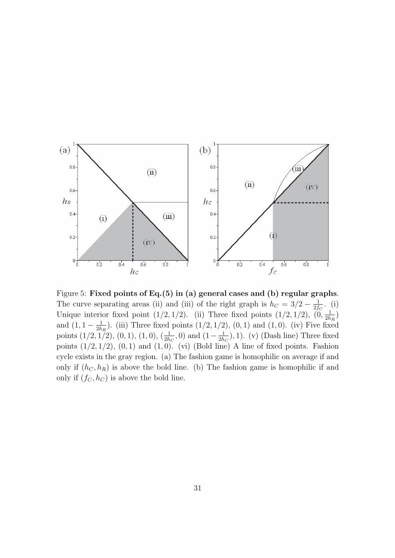
Figure 5: Fixed points of Eq.(5) in (a) general cases and (b) regular graphs.
The curve separating areas (ii) and (iii) of the right graph is hC = 3/2 − 12fC
. (i)
Unique interior fixed point (1/2, 1/2). (ii) Three fixed points (1/2, 1/2), (0, 12hR
)
and (1, 1− 12hR
). (iii) Three fixed points (1/2, 1/2), (0, 1) and (1, 0). (iv) Five fixed
points (1/2, 1/2), (0, 1), (1, 0), ( 12hC
, 0) and (1− 12hC
), 1). (v) (Dash line) Three fixed
points (1/2, 1/2), (0, 1) and (1, 0). (vi) (Bold line) A line of fixed points. Fashion
cycle exists in the gray region. (a) The fashion game is homophilic on average if and
only if (hC , hR) is above the bold line. (b) The fashion game is homophilic if and
only if (fC , hC) is above the bold line.
31
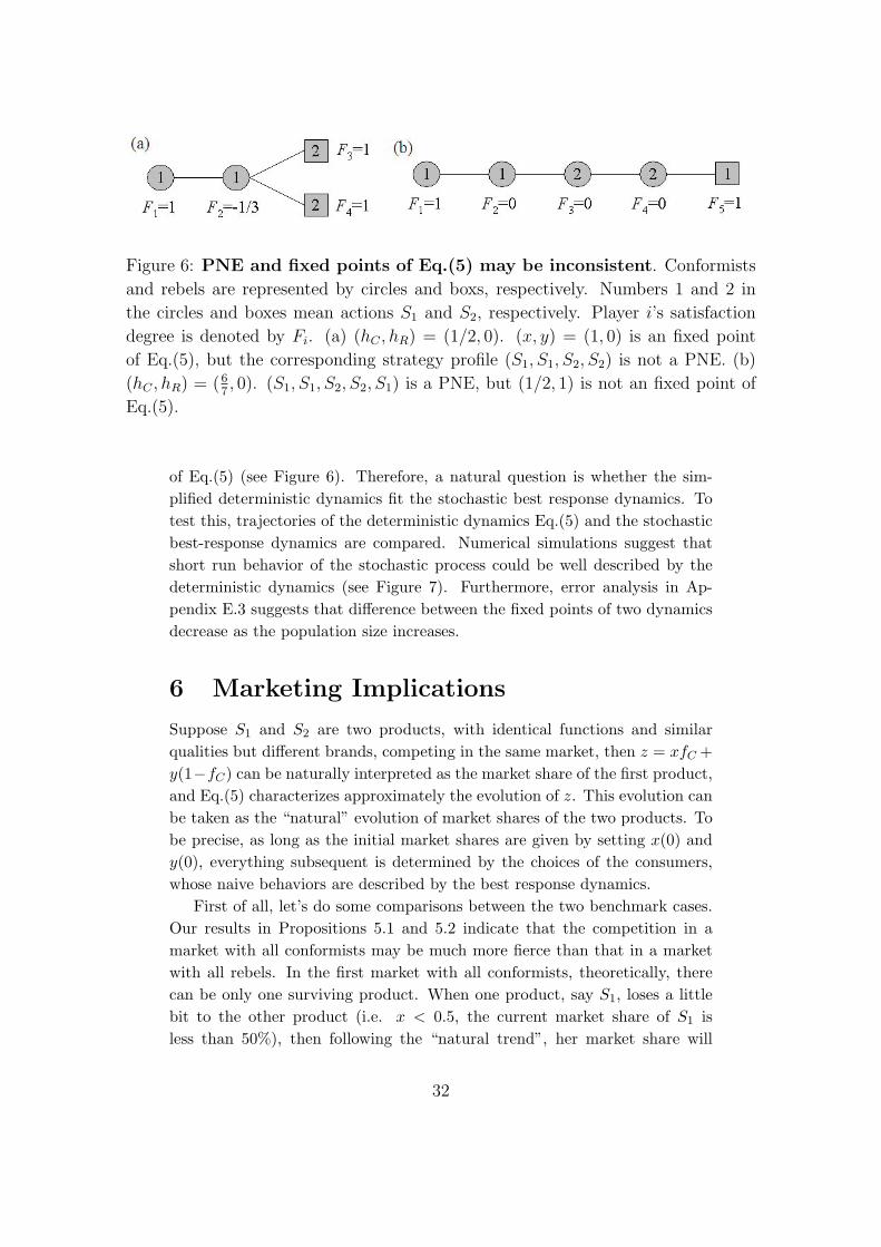
Figure 6: PNE and fixed points of Eq.(5) may be inconsistent. Conformists
and rebels are represented by circles and boxs, respectively. Numbers 1 and 2 in
the circles and boxes mean actions S1 and S2, respectively. Player i’s satisfaction
degree is denoted by Fi. (a) (hC , hR) = (1/2, 0). (x, y) = (1, 0) is an fixed point
of Eq.(5), but the corresponding strategy profile (S1, S1, S2, S2) is not a PNE. (b)
(hC , hR) = (67, 0). (S1, S1, S2, S2, S1) is a PNE, but (1/2, 1) is not an fixed point of
Eq.(5).
of Eq.(5) (see Figure 6). Therefore, a natural question is whether the sim-plified deterministic dynamics fit the stochastic best response dynamics. Totest this, trajectories of the deterministic dynamics Eq.(5) and the stochasticbest-response dynamics are compared. Numerical simulations suggest thatshort run behavior of the stochastic process could be well described by thedeterministic dynamics (see Figure 7). Furthermore, error analysis in Ap-pendix E.3 suggests that difference between the fixed points of two dynamicsdecrease as the population size increases.
6 Marketing Implications
Suppose S1 and S2 are two products, with identical functions and similarqualities but different brands, competing in the same market, then z = xfC +y(1−fC) can be naturally interpreted as the market share of the first product,and Eq.(5) characterizes approximately the evolution of z. This evolution canbe taken as the “natural” evolution of market shares of the two products. Tobe precise, as long as the initial market shares are given by setting x(0) andy(0), everything subsequent is determined by the choices of the consumers,whose naive behaviors are described by the best response dynamics.
First of all, let’s do some comparisons between the two benchmark cases.Our results in Propositions 5.1 and 5.2 indicate that the competition in amarket with all conformists may be much more fierce than that in a marketwith all rebels. In the first market with all conformists, theoretically, therecan be only one surviving product. When one product, say S1, loses a littlebit to the other product (i.e. x < 0.5, the current market share of S1 isless than 50%), then following the “natural trend”, her market share will
32
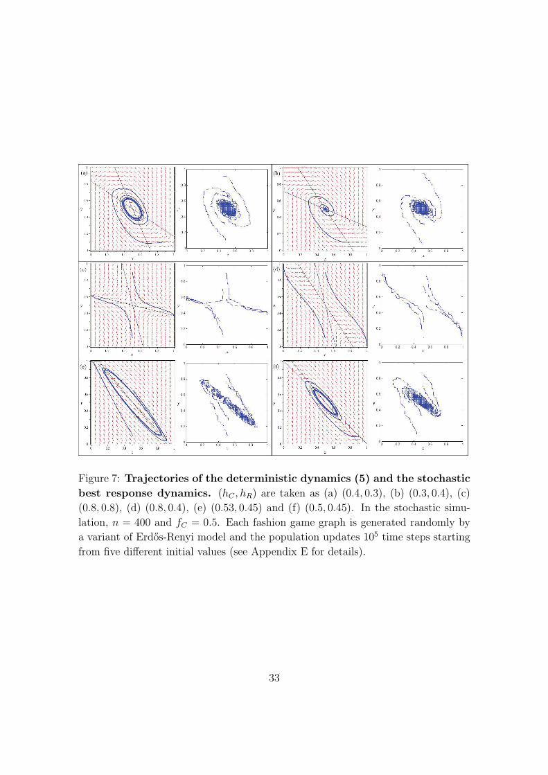
Figure 7: Trajectories of the deterministic dynamics (5) and the stochastic
best response dynamics. (hC , hR) are taken as (a) (0.4, 0.3), (b) (0.3, 0.4), (c)
(0.8, 0.8), (d) (0.8, 0.4), (e) (0.53, 0.45) and (f) (0.5, 0.45). In the stochastic simu-
lation, n = 400 and fC = 0.5. Each fashion game graph is generated randomly by
a variant of Erdos-Renyi model and the population updates 105 time steps starting
from five different initial values (see Appendix E for details).
33
eventually shrink to 0 (x = 0). And the more she loses, the more difficultfor her to reverse. There is a “Mattew Effect” or “positive feedback” behindthe dynamics, which is caused by the herd behavior of consumers (who are allconformists). To avoid the potential complete failure, the first producer maydecide to do more effort at the very beginning, say deeper price-cutting andmore intensive advertising and marketing. Being clear of the situation too, thesecond producer may do the same thing to keep her advantage, and thus thecompetition can be really cut-throat. For the market with all rebels, however,things are opposite. There is inherently an “anti-Mattew Effect” or “negativefeedback”, which is caused by the anti-herd behavior of consumers (who areall rebels). If the first producer is on the weak position at the beginning (i.e.y < 0.5), then she does not need to be worried at all, because the “naturaltrend” is on her side. Being clear of the situation too, the second producerhas no incentive to enhance marketing or advertising, or to cut price, sincethe more advantage she has in the market, the more difficult it is for her toobtain even bigger market share. Eventually, it is likely that both productssurvive and their market shares are half half (y = 0.5).
Although the above logic is hard to test directly, because practically it’squite challenging to say whether a consumer is a conformist or a rebel. How-ever, a fashion game with all conformists can be taken as a market for sellingproducts with strategic complements (say office softwares, online e-games,and social network services) and that with all rebels is mathematically equiv-alent to a market for selling products with strategic substitutes (say luxurygoods and fashionable clothing). Evidences can be found easily to supportthe proposition that competition in the first kind of markets are usually muchmore fierce than in the second one26. It should be noted also that the over-competition trend for a market selling products with strategic complementsis only true when the market is premature, that is, when there are still rel-atively many companies. However, once the market becomes mature, wheremost companies disappear and only one or two survives, competition can bereally insufficient, because new comers have no chance to get any share ofthe market at all. This is not true for markets selling products with strate-gic substitutes. New comers always has a chance, in fact, advantage, as longas they can provide new products. This may shed some new light on theanti-monopoly problem.
For the general situation where conformists and rebels coexist, i.e. 0 <
fC < 1, we can borrow some terms from signaling games to view our resultsagain. The second part of Theorem 5.1 tells us that when the social inter-
26For instance, some fashionable goods companies even do some “anti-marketing” behavior in thesense that they not advertise but try to hide the information of their products (Yoganarasimhan,2012a).
34
action structure satisfies homophily on average, then the natural evolution isto derive the system to boundary fixed points. In Case (iii), (0, 1) and (1, 0)are the two symmetric fixed points. This means that either S1 wins all theconformists but loses all the rebels, or the opposite. To put it another way,we are likely to have a “separating equilibrium”. In Case (ii), however, it ismore like a “semi-pooling equilibrium”: either all conformists choose S2 buta proportion of 1
2hRrebels choose S1 and the rest choose S2, or the opposite.
Similarly, when heterophily on average is satisfied, we may have a poolingequilibrium (Case (i)), or a separating equilibrium (Case (iv)).
7 Concluding Remarks
In this paper, we provide a new structural factor for the emergence of fashioncycle, suggesting that homophily, in general, is on the negative side of thisinteresting phenomenon. An immediate question is, if it is indeed the case,how to explain the conflict between the fact that fashion cycle is observedfrequently and homophily is also believed to exist quite universally? Honestly,we have no definite answer for the moment, and believe that further solidempirical research and possibly even controlled experiments are needed toinvestigate whether homophily or the opposite exists significantly. Only afterthat can we say that this is a valid question.
Research of this paper might also improve our understanding of fashionthrough the lens of complexity, because heterophily seems to be a more com-plex pattern than homophily. As already argued in Cao et al. (2013b), fashionseems unable to exist in a simple environment. When there is only one type ofagents, this is too dull. When the underlying interaction structure is a line ora ring, it is not complex enough. When the underlying interaction structureis complex enough but the configuration of the two types of agents exhibitshomophily, the environment is still too stylized and not complex enough.Combining with the fact that testing a general fashion game whether it pos-sesses a pure Nash equilibrium (PNE for short) or not is NP-hard (Cao andYang, 2011), we may have deeper understanding why fashion is so mysteriousand may conjecture that it is unpredictable27.
While the mathematical model we use is to attack the phenomenon offashion, and the terms in this paper are all about fashion, it may be actu-ally interpreted under other scenarios. In a paper in memory of Simmel andhis study on fashion, Benvenuto (2000) gave twelve other pairs of two oppo-site tendencies that are similar to imitation and distinction, namely, heredityand individual variation, universality and particularity, submission and sense
27As also noted in Cao et al. (2013), this conjecture is supported by industrial practices fromfast fashion. In Zara, for example, predicting the fashion trends has already been given up.
35

of power, duration and mutability, femininity and masculinity, stillness andmovement, receptivity and productivity, creation and destruction, DarwinianSelection and Darwinian Mutation, extensity and intensity, event and repeti-tion, accident and meaning.
Several more pairs can be thought out immediately, say obedience andrebelion, imitation and innovation. More technically, there are also some nat-ural pairs of terms, say positive feedback and negative feedback, coordinationand anti-coordination, strategic complements and strategic substitutes, su-permodular and submodular. So research on how the two competing forcesinteract with each other may have some quite universal meanings.
As to motivations, why people want to be like or different with the oth-ers goes also far beyond fashion. Young (2001) summarized three kinds ofreasons why people want to be like the others. The first, which he named“imitative conformity” or “pure conformity”, is exactly one side of fashion.People want to be like the others simply because otherwise they don’t feelgood. This seems to be the most unreasonable one among the three reasons.The second, which he named “instrumental conformity”, facilitates people’slivings. Just as argued by Young, “people drive on the same side of roadnot because it is fashionable, but because they want to avoid collisions.” Theforming of many conventions falls into this logic (Berninghaus and Schwalbe,1996; Young, 2001). The last, which he named “informational conformity”,says that “people adopt a behavior they observe around them because thedemonstration of effects”, i.e. they get useful information telling them thatthat particular behavior is good28.
As to why people want to be different with the others, we did not find asimilar classification in literature. Nevertheless, the analogous taxonomy isalmost immediate: pure deviation, instrumental deviation, and informationaldeviation. People may think that being different is fashionable, being differ-ent may give them a great convenience in living (say go shopping on Mondaymorning, choose a road to drive home that few people notice, etc.), and ob-serving that most people around her doing the same thing may tell her a veryimportant piece of information which makes her choose being different29.
Also, actions in this paper can also be safely taken as people’s opinions, soour research is closely related with the well studied field of social learning. Inthis field, BRD is also frequently used. Mathematically, (non-Bayesian, dis-crete opinion) network learning models are largely identical to the conformingside of the fashion game. Hence we hope that our research might enrich this
28The most theoretical studies following this logic are the mathematical models of “herd behav-ior”, and which on its own has grown into a rich theory called (Bayesian) social learning (Banerjee,1992; Bikchandani et. al., 1992; Acemoglu and Ozdaglar, 2010).
29For instance, when most people around you are buying stock, it is very likely that there is agreat bubble in the stock market and it is better for you to sell as soon as possible.
36
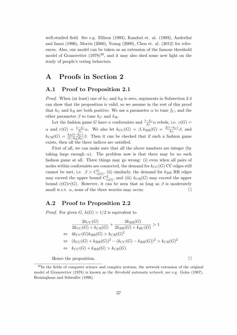
well-studied field. See e.g. Ellison (1993), Kandori et. al. (1993), Anderliniand Ianni (1996), Morris (2000), Young (2009), Chen et. al. (2012) for refer-ences. Also, our model can be taken as an extension of the famous thresholdmodel of Granovetter (1978)30, and it may also shed some new light on thestudy of people’s voting behaviors.
A Proofs in Section 2
A.1 Proof to Proposition 2.1
Proof. When (at least) one of hC and hR is zero, arguments in Subsection 2.4can show that the proposition is valid, so we assume in the rest of this proofthat hC and hR are both positive. We use a parameter α to tune fC , and theother parameter β to tune hC and hR.
Let the fashion game G have α conformists and 1−fCfC
α rebels, i.e. c(G) =
α and r(G) = 1−fCfC
α. We also let kCC(G) = β, kRR(G) = 2(1−hC)hC
β, and
kCR(G) = hR(1−hC)(1−hR)hC
β. Then it can be checked that if such a fashion gameexists, then all the three indices are satisfied.
First of all, we can make sure that all the above numbers are integer (bytaking large enough α). The problem now is that there may be no suchfashion game at all. Three things may go wrong: (i) even when all pairs ofnodes within conformists are connected, the demand for kCC(G) CC edges stillcannot be met, i.e. β > C2
c(G), (ii) similarly, the demand for kRR RR edgesmay exceed the upper bound C2
r(G), and (iii) kCR(G) may exceed the upperbound c(G)r(G). However, it can be seen that as long as β is moderatelysmall w.r.t. α, none of the three worries may occur.
A.2 Proof to Proposition 2.2
Proof. For given G, h(G) > 1/2 is equivalent to
2kCC(G)2kCC(G) + kCR(G)
+2kRR(G)
2kRR(G) + kRC(G)> 1
⇔ 4kCC(G)kRR(G) > kCR(G)2
⇔ (kCC(G) + kRR(G))2 − (kCC(G)− kRR(G))2 > kCR(G)2
⇔ kCC(G) + kRR(G) > kCR(G).
Hence the proposition.
30In the fields of computer science and complex systems, the network extension of the originalmodel of Granovetter (1978) is known as the threshold automata network, see e.g. Goles (1987),Berninghaus and Schwalbe (1996).
37
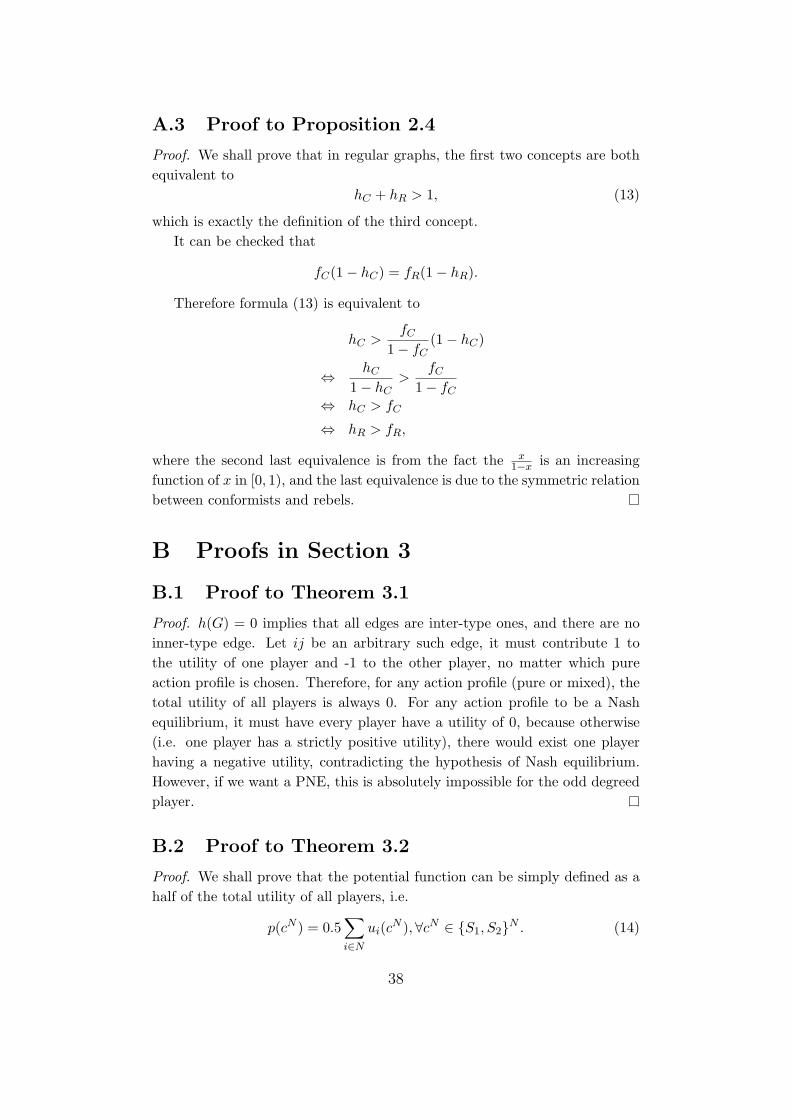
A.3 Proof to Proposition 2.4
Proof. We shall prove that in regular graphs, the first two concepts are bothequivalent to
hC + hR > 1, (13)
which is exactly the definition of the third concept.It can be checked that
fC(1− hC) = fR(1− hR).
Therefore formula (13) is equivalent to
hC >fC
1− fC(1− hC)
⇔ hC
1− hC>
fC
1− fC
⇔ hC > fC
⇔ hR > fR,
where the second last equivalence is from the fact the x1−x is an increasing
function of x in [0, 1), and the last equivalence is due to the symmetric relationbetween conformists and rebels.
B Proofs in Section 3
B.1 Proof to Theorem 3.1
Proof. h(G) = 0 implies that all edges are inter-type ones, and there are noinner-type edge. Let ij be an arbitrary such edge, it must contribute 1 tothe utility of one player and -1 to the other player, no matter which pureaction profile is chosen. Therefore, for any action profile (pure or mixed), thetotal utility of all players is always 0. For any action profile to be a Nashequilibrium, it must have every player have a utility of 0, because otherwise(i.e. one player has a strictly positive utility), there would exist one playerhaving a negative utility, contradicting the hypothesis of Nash equilibrium.However, if we want a PNE, this is absolutely impossible for the odd degreedplayer.
B.2 Proof to Theorem 3.2
Proof. We shall prove that the potential function can be simply defined as ahalf of the total utility of all players, i.e.
p(cN ) = 0.5∑
i∈N
ui(cN ),∀cN ∈ {S1, S2}N . (14)
38
Since h(G) = 1, we know that all edges are inner-type, and hence for anyaction profile, cN ∈ {S1, S2}N , and any edge ij ∈ E, i is liked by j if and onlyif j is liked by i, i.e.
i ∈ Lj(cN , G) ⇔ j ∈ Li(cN , G),∀cN ∈ {S1, S2}N . (15)
(15) indicates that
|Li(cN , G)| = ∣∣j ∈ Ni(G) : i ∈ Lj(cN , G)∣∣ ,∀cN ∈ {S1, S2}N , (16)
|Hi(cN , G)| =∣∣j ∈ Ni(G) : i ∈ Hj(cN , G)
∣∣ ,∀cN ∈ {S1, S2}N . (17)
Let aN ∈ {S1, S2}N be an arbitrary pure action profile. Suppose it is nota PNE, and i is unsatisfied with aN , then
ui(aN ) = |Li(aN , G)| − |Hi(aN , G)| < 0. (18)
Suppose w.l.o.g. that ai = S1, and let bN = (S2, a−i) be the pure action
profile derived by letting i switching her action from S1 to S2. Then
Li(aN , G) = Hi(bN , G),Hi(aN , G) = Li(aN , G). (19)
Combining (18) and (19), we have
ui(bN )− ui(aN ) = 2(|Hi(aN , G)| − |Li(aN , G)|) .
(16)(17)(19) imply that
{j ∈ Ni(G) : uj(bN ) > uj(aN )} = Hi(aN ),
{j ∈ Ni(G) : uj(bN ) < uj(aN )} = Li(aN ).
Because there is only one player, i, who switches action from aN to bN ,we know that each of i’s “enemy” in Hi(aN , G) gets a benefit of 2, and eachof her “friend” in Li(aN , G) gets a harm of 2. To be precise,
uj(bN )− uj(aN ) = 2,∀j ∈ Hi(aN , G),
uj(bN )− uj(aN ) = −2,∀j ∈ Li(aN , G).
By definition of (14) and the above arguments, we finally have
2(p(bN )− p(aN ))
=(ui(bN )− ui(aN )
)+
∑
j∈N\{i}
(uj(bN )− uj(aN )
)
=(ui(bN )− ui(aN )
)+
∑
j∈Ni(G)
(uj(bN )− uj(aN )
)
=(ui(bN )− ui(aN )
)+
∑
j∈Hi(aN ,G)
2−∑
j∈Li(aN ,G)
2
=(ui(bN )− ui(aN )
)+ 2(|Hi(aN , G)| − |Li(aN , G)|)
= 2(ui(bN )− ui(aN )
).
39

C Partial Potential Analysis: A General
Framework
To streamline the analysis, we shall present three concepts that are relax-ations of PNE, weak PNE component, PNE dominating set and strong PNEcomponent.
C.1 PNE components and PNE dominating set
Three elementary concepts from the graph theory will be used in the analysisof this subsection. The definitions below can be found in any text book ofgraph theory, say Bondy and Murty (1976).
Definition C.1 (Independent Set). Given a graph G = (N, E), we say thata subset of nodes S is an independent set if no pair of nodes in S are linkedto each other, i.e.
ij /∈ E, ∀i, j ∈ S.
Definition C.2 (Dominating Set). We say that S is a dominating set of G
if each node in N \ S has at least one neighbor in S, i.e.
Ni(G) ∩ S 6= ∅,∀i ∈ N \ S.
Definition C.3 (Induced Subgraph). Given a graph G = (N, E) and subsetof nodes S. Let E(S) be the inner edges of S, i.e.
E(S) = {ij : i, j ∈ S, ij ∈ E}.
Then G(S) = (S,E(S)) is called the induced subgraph of G derived by S.
When PNE is not guaranteed (as in the case of the fashion game), itis natural to ask how well can we “approximate” PNE. By approximate, wemean a pure action profile such that a large proposition of players are satisfied(i.e. have no incentive to deviate). If this proportion is 1, then we get exactlya PNE. Thus the largest possible such proportion is a natural measure ofPNE approximation, and the associated pure action profile is an extension ofPNE31.
Definition C.4 (Weak PNE Component). Let G = (N, (Ai)i∈N , (ui)i∈N ) bea strategic form game, and ∀S ⊆ N a subset of players. Suppose aS ∈ AS is
31It is well known that game theory, as a model of multiple player decision making, is a general-ization of optimization (i.e. single player decision making). With the above ideas, it can be takenas a special case of optimization too, because a Nash equilibrium corresponds to an action profilesuch that the number (or proportion) of satisfied players is maximized.
40
a pure action profile of S. If there exists bN\S ∈ AN\S such that no player inS has incentive to deviate in the action profile (aS , bN\S), i.e.
ui(ci, aS\{i}, bN\S) ≤ ui(aS , bN\S),∀i ∈ S,∀ci ∈ Ai \ {ai},
we call aS a weak PNE component (w.r.t. bN\S).
Suppose for the moment that G is a network game and the underlyinggraph is a spatial one32, then S possesses a weak PNE component means thatthe local region consisting of players in S can be relatively stable. Not onlythat it is locally stable at some fixed moment, but also that this local stabilitycan last for some time, because the “invasion” needs a process.
When there exists aS ∈ AS such that aN is a weak PNE component, wesay that S possesses a weak PNE component. A weak PNE component aS iscalled maximal if there is no j ∈ N \ S and bj ∈ Aj such that (aS , bj) is alsoa weak PNE component.
Proposition C.1. Weak PNE components have the following properties.(a) Suppose G is a strategic game. If aS is a maximal weak PNE componentw.r.t. bN\S, then no player in N \ S is satisfied with the pure action profile(aS , bN\S).(b) Suppose G is a network game. If S is an independent set, then S possessesa weak PNE component.(c) Suppose G is a network game. If S possesses a weak PNE component, letNS(G) be the union of neighbor sets of players in S, i.e.
NS(G) =⋃
i∈S
Ni(G),
and let I be an independent set of the induced subgraph G(N \ (S ∪NS(G))),then S ∪ I possesses a weak PNE component of G.(d) Suppose G is a network game. If S possesses a maximal weak PNE com-ponent, then S is a dominating set of G.
Proof. Part (a) is obvious, because otherwise the hypothesis that aS is maxi-mal would be violated.
We shall prove a result stronger than (b). Suppose now S is an independentset, and let bN\S be an arbitrary pure action profile of N \ S. Fix bN\S , welet players in S choose actions they like most one by one (in an arbitraryorder). A critical observation of any network game is that the payoff of anyplayer is affected only by the actions of her neighbors (and the action of herown). Since no pair of players in S are neighboring to each other, we know
32By “spatial”, we mean that players are located on a plane or the surface of a ball, and two play-ers are neighbor to each other only if they are geographically near. In graph theory, correspondingconcepts are Euclidian graph and planar graph.
41
that the actions of later players do not affect the payoffs of the earlier players.Therefore, all players in S will eventually be satisfied, and hence S possessesa weak PNE component w.r.t. bN\S .
To prove (c), suppose aS is a weak PNE component w.r.t. bN\S . Similarto the proof of (b), we fix aS and let the players in I choose a best responseone by one (in an arbitrary). Let their choices be cI . I is an independent setof G(N \ (S ∪NS(G))) indicates that none of the players in S will be affected,and neither will the deviation of later players in I affect the earlier ones. Thus(aS , cI) is a weak PNE component w.r.t. bN\(S∪I).
(d) is valid directly from (c), because S is a dominating set of G if andonly if N \ (S ∪NS(G)) = ∅.
Proposition C.2. Let G = (N, (Ai)i∈N , (ui)i∈N ) be a strategic form game.If each players has exactly m actions in game G, i.e. |Ai| ≤ m, ∀i ∈ N , thentheir exists S ⊆ N , such that
|S| ≥ n/m,
and S possesses a weak PNE component.
Proof. We prove via a simple application of the probabilistic method (c.f.Alon and Spencer, 2007). Let each player choose a pure action uniformlyrandomly, then the probability that player i is satisfied is at least 1/|Ai| ≥1/m. Therefore, the expected number of satisfied players is at least n/m, andhence there must exist a pure action profile where at least n/m players aresatisfied (because otherwise the expected number of satisfied players wouldbe strictly less than n/m). This completes the proof.
The above proposition tells us that when the pure action space of eachplayer is small, then we must have weak PNE component with a nontrivialsize.
Definition C.5 (Strong PNE component). Let G = (N, (Ai)i∈N , (ui)i∈N ) beany strategic form game. ∀S ⊆ N , aS ∈ AS is called a strong PNE componentof G if and only if for all aN\S ∈ AN\S, no player in S has incentive to deviatein the action profile (aS , aN\S).
It is easy to construct examples to show that Proposition C.1 and Propo-sition C.2 do not hold for strong PNE component. However, it has a specialproperty of its own.
Proposition C.3. Let G be any strategic game. If X and Y are two disjointplayer sets, aX and aY are two strong PNE components, then (aX , aY ) is alsoa strong PNE component.
42

Proof. ∀cN\(X∪Y ) ∈ AN\(X∪Y ), then aX is a strong PNE components meansthat all players are satisfied in in action profile (aX , bY , cN\(X∪Y ). For thesame reason, players in Y have no incentive to deviate either. Hence theproposition.
Note that the above property is not held by weak PNE component. Tosee this, it is enough to observe that any single set possesses a weak PNEcomponent. If on the contrary the above property holds, then we would getthat the whole set of N , which is a union of single player sets, possesses aweak PNE too. This means we would derive that PNE exists for any strategicgame, which is obviously impossible.
Definition C.6 (PNE Dominating Set). Let G = (N, (Ai)i∈N , (ui)i∈N ) be astrategic form game and S ⊆ N a subset of players. We say S is a PNEdominating set if for each bN\S, S possesses a weak PNE component w.r.t.bN\S.
The definition of NS(G) in Proposition C.1 is still valid in the followingproposition.
Proposition C.4. Let G be any network game.(a) Any independent set of G is a PNE dominating set.(b) If two disjoint player sets X and Y are both PNE dominating sets, noplayer in X has any neighbor in Y , and no player in Y has any neighbor inX, i.e.
NX(G) ∩ Y = ∅, NY (G) ∩X = ∅, (20)
then X ∪ Y is also a PNE dominating set.(c) If S is a PNE dominating set, and let I be an independent set of theinduced subgraph G(N \ (S ∪NS(G))), then S ∪ I is a PNE dominating set ofG.(d) If S is a maximal PNE dominating set, then it must be a dominating setof the underlying graph.
Proof. (a) is an improvement of Proposition C.1(b), and is already impliedin the proof to Proposition C.1(b). (d) is a direct implication of PropositionC.1(d). (c) is implied in the combination of (a) and (b). So we are left toshow that (b) is true.
Conditions in (20) tell us that the payoffs of players in X are affectedonly by players in N \ (X ∪ Y ) (and their own actions), but not by Y , andthe payoffs of Y are not affected by X. Due to the above reason and thehypothesis that X and Y are both PNE dominating sets, for arbitrary actionprofile of N \ (X ∪ Y ), we can make all the players in X ∪ Y be satisfied, andhence (b) is true.
43
It is easy to show that conditions in (20) are indispensable. The observa-tions below can also easily shown to be true, (i) a PNE is the largest possiblestrong PNE component, (ii) when S possesses a strong PNE component, itmust be a PNE dominating set, (iii) any PNE dominating set must possess aweak PNE component, (iv) when PNE eixsts, the sets of PNEs, largest strongPNE components and largest weak PNE components all coincide.
C.2 Partial potential games
It turns out that partial potential argument is very powerful in proving theexistence of certain particular form weak/strong PNE components and PNEs.To ease the presentation, we need to first present the exact meaning of partialpotential games.
Definition C.7 (Partial Potential Games33). Let G = (N, (Ai)i∈N , (ui)i∈N )be a strategic form game. S is a subset of players and bN\S ∈ AN\S a pureaction profile of N \ S. G(bN\S) = (S, (Ai)i∈S , (ui(bN\S))i∈S) is the reducedgame of G derived from fixing the actions of players in N \ S as bN\S, where
ui(bN\S)(aS) = ui(aS , bN\S),∀i ∈ S,∀aS ∈ AS .
We say that G is a partial potential game w.r.t. bN\S if the reduced gameG(bN\S) is a potential game.
We say that G is a partial potential game w.r.t. N \ S if it is a partialpotential game w.r.t. all bN\S ∈ AN\S.
The close relations between partial potential games and PNE componentsand PNE dominating sets are expressed in the following theorem.
Theorem C.1. Let G = (N, (Ai)i∈N , (ui)i∈N ) be a strategic form game. S isa subset of players.(a) If there exists bN\S ∈ AN\S such that G is a partial potential game w.r.t.bN\S, then S possesses a weak PNE component.(b) If G is a partial potential game w.r.t. N \S, then S is a PNE dominatingset.(c) If bN\S ∈ AN\S is a strong PNE component of G, and G is a partialpotential game w.r.t. bN\S, then G possesses a PNE.
Proof. G is a partial potential game w.r.t. bN\S indicates that the reducedgame G(bN\S) possesses a PNE, which is a weak PNE component of N \ S.Hence (a) is true. Recall Definition C.6 and Definition C.7, (b) is an immediateimplication of (a).
To prove (c), let cS be a PNE for the reduced game G(bN\S). Then(cS , bN\S) is a PNE for G.
33We do not distinguish between exact potential game, weighted potential game, and ordinalpotential game. In fact, our results are valid for any particular kind of potential games.
44
C.3 Application on the fashion game
For the fashion game, since each player has exactly 2 actions, we get imme-diately from Proposition C.2 that the largest weak PNE component consistsof at least a half of all the players. In fact, using the partial potential argu-ments introduced in the previous subsection, we have the following strongerand more concentrate results.
Theorem C.2. Suppose G = (N, E, T ) is a fashion game.(a) G is a partial potential game w.r.t. R, and hence C is a PNE dominatingset.(b) G is a partial potential game w.r.t. C, and hence R is a PNE dominatingset.(c) Let H∗ be the set of players that have a homophily index of 1, i.e.
H∗ = {j ∈ N : hi(G) = 1}, (21)
then G is a partial potential game w.r.t. N \ H∗, and hence H∗ is a PNEdominating set.(d) Let X ∈ {C, R,H∗}, and I∗(X) be an independent set of the inducedsubgraph G(N \X), then X ∪ I∗(X) is also a PNE dominating set.
Proof. To prove (a)(b)(c), we need a simple property of potential games. Sup-pose G = (N, (Ai)i∈N , (ui)i∈N ) is a potential game, then G′ = (N, (Ai)i∈N , (vi)i∈N )is also a potential game, where there exists a constant δi such that
vi(aN ) = ui(aN ) + δi,∀i ∈ N, ∀aN ∈ AN . (22)
This property is true because the preferences of all players in G′ are exactlythe same as in G.
To prove (a), let aR be an arbitrary pure action profile of the rebel setR. We construct a new fashion game G′(aR) from the reduced game G(aR)by letting the payoff of each player in G′(aR) be the number of neighbors shelikes minus that she hates. Then G′(aR) is a fashion game and there existsconstant δi such that (22) holds. Since G′(aR) is a fashion game with onlyconformists, we know from Theorem 3.2 that it is a potential game. Henceusing the above property we know that G(aR) is also a potential game.
Similar to the proof to (a), (b) and (c) can be shown to be true using acombination of the above property and Theorem 3.2. (d) is a simple applica-tion of Proposition C.4(d).
Proposition C.5. Let G = (N, E, T ) be a fashion game.(a) If G is strong conformist homophily, then C possesses a strong PNE com-ponent.(b) If G is strong rebel homophily, then R possesses a strong PNE component.
45
Proof. (a) is true because we can simply let all the conformist choose S1. (b)is also easy, because we can let players in R1 choose S1 and players in R2
choose S2, where R1 and R2 are the same as in Definition
Combining Theorem C.1(c), Theorem C.2(a)(b), and Proposition C.5, wehave the main result of Theorem 4.1.
D Proofs in Section 5
D.1 Derivation of Eq.(4)
For convenience, we call C1, C2, R1 and R2 types 1, 2, 3 and 4, respectively.Denote the probability density of the four types at time t by x = (fCx, fC(1−x), (1−fC)y, (1−fC)(1−y)). For given x, the probability Tij(x) that a playerof type i changes to type j can be calculated.
T21 = P (n1C → n1
C + 1), T22 = 1− T21,
T12 = P (n1C → n1
C − 1), T11 = 1− T12,
T43 = P (n1R → n1
R + 1), T44 = 1− T43,
T34 = P (n1R → n1
R − 1), T33 = 1− T34,
(23)
and Tij = 0 for others.A Fokker-Planck equation for the probability density ρ(x) can be derived
by applying Kramers-Moyal expansion (Traulsen et al., 2005; Traulsen et al.,2006):
ρ(x) = −3∑
k=1
∂
∂xkρ(x)ak(x) + 1/2
3∑
j,k=1
∂2
∂xk∂xjρ(x)bjk(x), (24)
where drift terms are given by
ak(x) =4∑
j=1
(Tjk(x)− Tkj(x)
), (25)
and the diffusion matrix is given by
bjk(x) =1n
(−Tjk(x)− Tkj(x) + δjk
4∑
l=1
(Tjl(x) + Tlj(x)
))
. (26)
Since the noise arises only from stochastic updating and is therefore notcorrelated in time, the Ito calculus can be applied to derive a Langevin equa-tion describing the time evolution of x (Traulsen et al., 2006). Eq.(24) corre-sponds to the stochastic replicator-mutator equation
xk = ak(x) +3∑
j=1
ckj(x)ξj(t), (27)
46
where ckj is defined by∑3
l=1 ckl(x)clj(x) = bkj(x) and each element of thevector ξ is Gaussian white noise with unit variance. Therefore, cij vanishesat a rate of 1√
nas n →∞. From Eq.(23),
a1(x) = T21(x)− T12(x),a2(x) = T12(x)− T21(x),a3(x) = T43(x)− T34(x).
Notice that x1 + x2 = fC , Eq.(27) could be simplified as{
x1 = T21(x)− T12(x) +∑3
j=1 c1j(x)ξj(t),x3 = T43(x)− T34(x) +
∑3j=1 c3j(x)ξj(t).
This yields Eq.(4).
D.2 Stability conditions in Table 1
At the interior fixed point (1/2, 1/2), Jacobian matrix of Eq.(5) is given by(
−2φ′(0)hC −2φ′(0)(1− hC)2φ′(0)(1− hR) 2φ′(0)hR
)(28)
with eigenvalues
λ1,2 = φ′(0)(hR − hC ±
√(hR − hC)2 − 4(1− hR − hC)
). (29)
(1/2, 1/2) is locally asymptotically stable if and only if all eigenvalues havenegative real parts, i.e., hR − hC > 0 and hC + hR < 1. In particular, fromEq.(A.3), stability conditions for regular networks are fC < 1/2 and hC < fC .
We next study the stabilities of boundary fixed points for each case.• Case (i). As shown in Table 1, boundary fixed point does not exist in
this case.• Case (ii). The interior fixed point (1/2, 1/2) must be unstable since
hC + hR > 1. Eq.(5) has two boundary fixed points (0, 1/(2hR)) and (1, 1 −1/(2hR)). Jacobian matrix at (0, 1/(2hR)) is
(−φ(F (C1)) 0
2φ′(0)(1− hR) 2φ′(0)hR
), (30)
where F (C1) = 1−hC−hRhR
< 0. Two eigenvalues of Eq.(30) are λ1 = −φ(F (C1))and λ2 = 2φ′(0)hR < 0. Notice that both of them are negative, (0, 1/(2hR)) islocally asymptotically stable. Similarly, (1, 1−1/(2hR)) is also locally asymp-totically stable.
47
• Case (iii). The interior fixed point (1/2, 1/2) must be unstable sincehC +hR > 1. Eq.(5) has two boundary fixed points (0, 1) and (1, 0). Jacobianmatrix at (0, 1) is
(−φ(F (C1)) 0
0 −φ(F (R2))
), (31)
where F (C1) = 1 − 2hC < 0 and F (R2) = 2hR − 1 < 0. Two eigenvalues ofEq.(31) are λ1 = −φ(F (C1)) < 0 and λ2 = −φ(F (R2)) < 0. Notice that bothof them are negative, (0, 1) is locally asymptotically stable. Similarly, (1, 0)is also locally asymptotically stable.
• Case (iv). The interior fixed point (1/2, 1/2) must be unstable sincehC > hR. Eq.(5) has four boundary fixed points (0, 1), (1, 0), (1/(2hC), 0) and(1− 1/(2hC), 1). Similarly to Case (iii), (0, 1) and (1, 0) are locally asymptot-ically stable. Jacobian matrix at (1/(2hC), 0) is
(−2φ′(0)hC −2φ′(0)(1− hC)
0 −φ(F (R1))
), (32)
where F (R1) = hC+hR−1hC
< 0. Two eigenvalues of Eq.(32) are λ1 = −2φ′(0)hC >
0 and λ2 = −φ(F (R1)) < 0. Thus, (1/(2hC), 0) is an unstable saddle point.Similarly, (1− 1/(2hC), 1) is also a saddle point.
• Case (v). The interior fixed point (1/2, 1/2) must be unstable sincehC > hR. Eq.(5) has two boundary fixed points (0, 1) and (1, 0). Jacobianmatrix at (0, 1) is
(−2φ′(0)hC −2φ′(0)(1− hC)
0 −φ(F (R2))
), (33)
where F (R2) = 2hR−1 < 0. Two eigenvalues of Eq.(33) are λ1 = −2φ′(0)hC >
0 and λ2 = −φ(F (R2)) < 0. Thus, (0, 1) is an unstable saddle point. Simi-larly, (1, 0) is also a saddle point.
D.3 Proof to Theorem 5.1
In this section, we investigate the global behaviors of Eq.(5) for six cases byzero-isoclines. On x − y plane, zero-isoclines for dx
dt = 0 and dydt = 0 are
respectively
Lx : y =1
2(1− hC)− hC
1− hCx,
Ly : y = 1/(2hR)− 1− hR
hRx.
Note that in Figure 7, blue lines are Lx and blacks ones are Ly. dxdt > 0(< 0)
for points above (below) Lx and dydt < 0(> 0) for points above (below) Ly.
48
x− y plane is then divided into four regions (except Case (vi)) and two lineshave a unique intersection (1/2, 1/2). For convenience, we denote the slopesof the two zero-isoclines Lx and Ly by kx and ky, respectively.
• Case (i): kx > −1 and kx > ky. Graphically, trajectories of Eq.(5) moveclockwise around (1/2, 1/2) and go always from boundaries. If the interiorfixed point is unstable, Eq.(5) must have a periodic solution (See Figure 7(a)).If (1/2, 1/2) is locally stable, one may guess that it is also globally attractive.However, this is not true. Depending on the changing probability φ, Eq.(5)may have more than one periodic solution. We show one example that theinterior fixed point is globally attractive in Figure 7(b) and another examplethat Eq.(5) has two periodic solutions in Figure 7(e).
• Case (ii): ky > −1 and ky > kx. The interior fixed point (1/2, 1/2)is unstable and two boundary fixed points (0, 1
2fR|R) and (1, 1 − 1
2fR|R) are
locally asymptotically stable. In this case, existence of a periodic solution isimpossible since vector fields in four regions can not form a cycle (see Figure7(c)).
• Case (iii): kx − 1 and ky < −1. The interior fixed point (1/2, 1/2) isunstable and two boundary fixed points (0, 1) and (1, 0) are locally asymptot-ically stable. The phase portrait in this case looks like case (ii), where Eq.(5)have no periodic solution. (See Figure 7(d))
• Case (iv): −1 > kx > ky. (0, 1) and (1, 0) are locally asymptoticallystable, and ( 1
2fC|C, 0) and (1− 1
2fC|C, 1) are saddle points. The global dynamic
behavior could be very complicated. Eq.(5) may have two periodic solutionsif the interior fixed point (1/2, 1/2) is unstable (see Figure 7(e)).
• Case (v): −1 = kx > ky. (0, 1) and (1, 0) are saddle points. Similarly ascase (i), trajectories of Eq.(5) move clockwise around (1/2, 1/2). If the interiorfixed point (1/2, 1/2) is unstable, Eq.(5) must have a periodic solution. (SeeFigure 7(f)) On the other hand, even if the interior fixed point is locally stable,Eq.(5) may have two periodic solutions.
• Case (vi): kx = ky, i.e., two zero-isoclines are identical, and all pointson the line are fixed points. In this case, trajectories of Eq.(5) converge tothe line y = 1
2(1−hC) − hC1−hC
x.
E Numerical Simulations
Since the deriving of Eq.(5) applied pair approximation and diffusion approx-imation, a natural question is whether this simplification is appropriate. Toanswer this question, we compare the trajectories of the deterministic dynam-ics and the trajectories of the stochastic best-response dynamics for fashiongames with different homophily indices and population sizes. In subsectionD.1, we introduce a variant of Erdos-Renyi model that could generate fash-
49
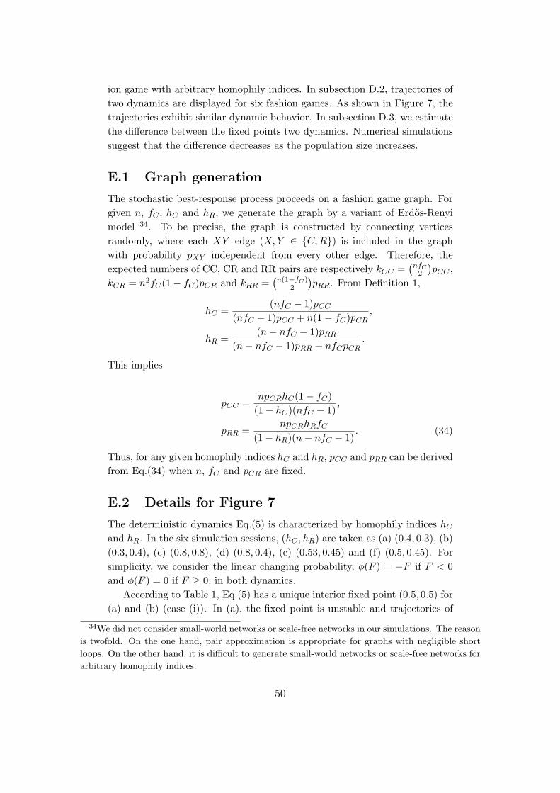
ion game with arbitrary homophily indices. In subsection D.2, trajectories oftwo dynamics are displayed for six fashion games. As shown in Figure 7, thetrajectories exhibit similar dynamic behavior. In subsection D.3, we estimatethe difference between the fixed points two dynamics. Numerical simulationssuggest that the difference decreases as the population size increases.
E.1 Graph generation
The stochastic best-response process proceeds on a fashion game graph. Forgiven n, fC , hC and hR, we generate the graph by a variant of Erdos-Renyimodel 34. To be precise, the graph is constructed by connecting verticesrandomly, where each XY edge (X, Y ∈ {C, R}) is included in the graphwith probability pXY independent from every other edge. Therefore, theexpected numbers of CC, CR and RR pairs are respectively kCC =
(nfC2
)pCC ,
kCR = n2fC(1− fC)pCR and kRR =(n(1−fC)
2
)pRR. From Definition 1,
hC =(nfC − 1)pCC
(nfC − 1)pCC + n(1− fC)pCR,
hR =(n− nfC − 1)pRR
(n− nfC − 1)pRR + nfCpCR.
This implies
pCC =npCRhC(1− fC)
(1− hC)(nfC − 1),
pRR =npCRhRfC
(1− hR)(n− nfC − 1). (34)
Thus, for any given homophily indices hC and hR, pCC and pRR can be derivedfrom Eq.(34) when n, fC and pCR are fixed.
E.2 Details for Figure 7
The deterministic dynamics Eq.(5) is characterized by homophily indices hC
and hR. In the six simulation sessions, (hC , hR) are taken as (a) (0.4, 0.3), (b)(0.3, 0.4), (c) (0.8, 0.8), (d) (0.8, 0.4), (e) (0.53, 0.45) and (f) (0.5, 0.45). Forsimplicity, we consider the linear changing probability, φ(F ) = −F if F < 0and φ(F ) = 0 if F ≥ 0, in both dynamics.
According to Table 1, Eq.(5) has a unique interior fixed point (0.5, 0.5) for(a) and (b) (case (i)). In (a), the fixed point is unstable and trajectories of
34We did not consider small-world networks or scale-free networks in our simulations. The reasonis twofold. On the one hand, pair approximation is appropriate for graphs with negligible shortloops. On the other hand, it is difficult to generate small-world networks or scale-free networks forarbitrary homophily indices.
50
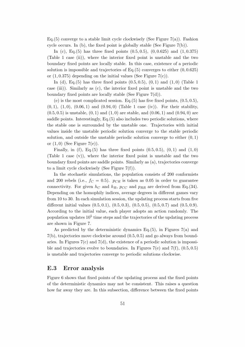
Eq.(5) converge to a stable limit cycle clockwisely (See Figure 7(a)). Fashioncycle occurs. In (b), the fixed point is globally stable (See Figure 7(b)).
In (c), Eq.(5) has three fixed points (0.5, 0.5), (0, 0.625) and (1, 0.375)(Table 1 case (ii)), where the interior fixed point is unstable and the twoboundary fixed points are locally stable. In this case, existence of a periodicsolution is impossible and trajectories of Eq.(5) converges to either (0, 0.625)or (1, 0.375) depending on the initial values (See Figure 7(c)).
In (d), Eq.(5) has three fixed points (0.5, 0.5), (0, 1) and (1, 0) (Table 1case (iii)). Similarly as (c), the interior fixed point is unstable and the twoboundary fixed points are locally stable (See Figure 7(d)).
(e) is the most complicated session. Eq.(5) has five fixed points, (0.5, 0.5),(0, 1), (1, 0), (0.06, 1) and (0.94, 0) (Table 1 case (iv)). For their stability,(0.5, 0.5) is unstable, (0, 1) and (1, 0) are stable, and (0.06, 1) and (0.94, 0) aresaddle points. Interestingly, Eq.(5) also includes two periodic solutions, wherethe stable one is surrounded by the unstable one. Trajectories with initialvalues inside the unstable periodic solution converge to the stable periodicsolution, and outside the unstable periodic solution converge to either (0, 1)or (1, 0) (See Figure 7(e)).
Finally, in (f), Eq.(5) has three fixed points (0.5, 0.5), (0, 1) and (1, 0)(Table 1 case (v)), where the interior fixed point is unstable and the twoboundary fixed points are saddle points. Similarly as (a), trajectories convergeto a limit cycle clockwisely (See Figure 7(f)).
In the stochastic simulations, the population consists of 200 conformistsand 200 rebels (i.e., fC = 0.5). pCR is taken as 0.05 in order to guaranteeconnectivity. For given hC and hR, pCC and pRR are derived from Eq.(34).Depending on the homophily indices, average degrees in different games varyfrom 10 to 30. In each simulation session, the updating process starts from fivedifferent initial values (0.5, 0.1), (0.5, 0.3), (0.5, 0.5), (0.5, 0.7) and (0.5, 0.9).According to the initial value, each player adopts an action randomly. Thepopulation updates 105 time steps and the trajectories of the updating processare shown in Figure 7.
As predicted by the deterministic dynamics Eq.(5), in Figures 7(a) and7(b), trajectories move clockwise around (0.5, 0.5) and go always from bound-aries. In Figures 7(c) and 7(d), the existence of a periodic solution is impossi-ble and trajectories evolve to boundaries. In Figures 7(e) and 7(f), (0.5, 0.5)is unstable and trajectories converge to periodic solutions clockwise.
E.3 Error analysis
Figure 6 shows that fixed points of the updating process and the fixed pointsof the deterministic dynamics may not be consistent. This raises a questionhow far away they are. In this subsection, difference between the fixed points
51
of two dynamics are compare for games with different homophily indices andpopulation sizes.
We run two series of simulations. In the first series, population consistsof 50 conformists and 50 rebels, and in the second series, population consistsof 200 conformists and 200 rebels . In each series, we generate 1210 fashiongames for 121 different homophily indices (hC , hR) (10 games per (hC , hR)),where hC and hR vary from 0 to 1 with interval 0.1. For each game, werun the stochastic updating process 105 time steps from 25 different initialvalues (x, y) (so they are 25 trajectories), where x and y vary from 0.1 to0.9 with interval 0.2. In most of cases that partial potential conditions aresatisfied, the updating process stops at a PNE (denoted by (x, y)). If not,we use the average of the last 104 steps to represent the fixed point of thetrajectory. On the other hand, denote the limit point of the trajectory of thedeterministic dynamics starting from the same initial value by (x, y). If thetrajectory converges to a limit cycle, let (x, y) = (1/2, 1/2) which is the timeaverage of the limit cycle. For each initial value, (absolute) difference betweenthe fixed points of two dynamics is given by ε = max{|x− x|, |y− y|}. Finally,define the difference for homophily indices (hC , hR) by the average of its 250samples (10 games × 25 initial values per game).
Figure 8 shows the difference between the fixed points of two dynamics for121 different homophily indices. Overall, difference is decreasing in populationsize. When n = 100, the average difference is 0.077 (Figure 8(a)) and whenn = 400, the average difference is only 0.037 (Figure 8(b)). This matchesthe prediction of diffusion approximation: difference drops by one half as thepopulation size increases four times.
In both series, difference is large for homophily indices close to lineshR + hC = 1, hC = 0.5 and hR = 0.5. An explanation is that homophilyindices on the three lines are bifurcation values of the deterministic dynamics.Therefore, trajectories of the updating process are very sensitive to stochasticfactors. In contrast, difference is very small for homophily indices far fromthese lines. In this case, dynamic behavior of the updating process could bewell approximated by the deterministic dynamics.
References
[1] C. Anderson. Recycle, Reuse, Bury or Burn? Bristol: SOFA Project, 1999.
[2] R. Aharoni, E.C. Milner, et. al., Unfriendly partitions of a graph. Journalof Combinatorial Theory, Series B 50(1) (1990): 1-10.
[3] Acerbi A, Ghirlanda S, Enquist M (2012) The logic of fashion cycles. PLoSONE, 7(3): e32541. doi:10.1371/journal.pone.0032541
52
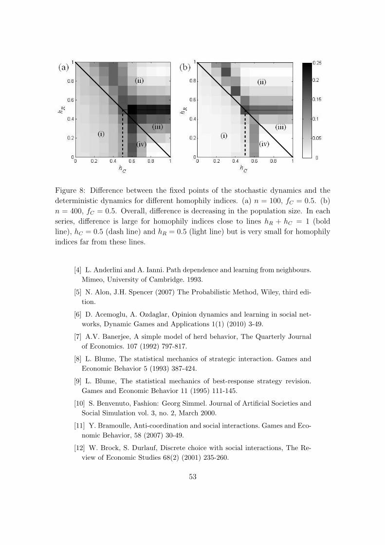
Figure 8: Difference between the fixed points of the stochastic dynamics and the
deterministic dynamics for different homophily indices. (a) n = 100, fC = 0.5. (b)
n = 400, fC = 0.5. Overall, difference is decreasing in the population size. In each
series, difference is large for homophily indices close to lines hR + hC = 1 (bold
line), hC = 0.5 (dash line) and hR = 0.5 (light line) but is very small for homophily
indices far from these lines.
[4] L. Anderlini and A. Ianni. Path dependence and learning from neighbours.Mimeo, University of Cambridge. 1993.
[5] N. Alon, J.H. Spencer (2007) The Probabilistic Method, Wiley, third edi-tion.
[6] D. Acemoglu, A. Ozdaglar, Opinion dynamics and learning in social net-works, Dynamic Games and Applications 1(1) (2010) 3-49.
[7] A.V. Banerjee, A simple model of herd behavior, The Quarterly Journalof Economics. 107 (1992) 797-817.
[8] L. Blume, The statistical mechanics of strategic interaction. Games andEconomic Behavior 5 (1993) 387-424.
[9] L. Blume, The statistical mechanics of best-response strategy revision.Games and Economic Behavior 11 (1995) 111-145.
[10] S. Benvenuto, Fashion: Georg Simmel. Journal of Artificial Societies andSocial Simulation vol. 3, no. 2, March 2000.
[11] Y. Bramoulle, Anti-coordination and social interactions. Games and Eco-nomic Behavior, 58 (2007) 30-49.
[12] W. Brock, S. Durlauf, Discrete choice with social interactions, The Re-view of Economic Studies 68(2) (2001) 235-260.
53
[13] Berger, J., B. Ho, et al. (2011). “Identity Signaling with Social Capital:A Model of Symbolic Consumption.” Johnson School Research Paper SeriesNo.27-2011.
[14] S. Bikchandani, B.D. Hirshleifer, I. Welch, A Theory of fads, fashion,custom and cultural change as informational cascades, Journal of PoliticalEconomy, 100(5) (1992) 992-1026.
[15] Y. Bramoulle, D. Lopez-Pintado, S. Goyal, F. Vega-Redondo, Networkformation and anti-coordination games, International Journal of Game The-ory 33(1) (2004) 1-19.
[16] Bondy, J., Murty, U., 1976. Graph Theory with Applications. North-Holland, New York.
[17] S.K. Berninghaus, U. Schwalbe, Conventions, local interaction, and au-tomata networks, Journal of Evolutionary Economics, 6 (1996) 297-312.
[18] C. Cannings. The Majority and Minority Models on Regular and RandomGraphs. International Conference on Game Theory for Networks, 2009.
[19] A. Chai, P.E. Earl and J. Potts. Fashion, growth and welfare: an evolu-tionary approach. Advances in Austrian Economics, 10, 2007, 187-207.
[20] Currarini, S., M. O. Jackson, et al. An economic model of friendship:Homophily, minorities, and segregation. Econometrica 77(4) (2009): 1003-1045.
[21] T. Cooper and K. Mayers. Prospects for Household Appliances. Halifax:Urban Mines Ltd, 2000.
[22] D. Challet, M. Marsili and Y.C. Zhang. Minority Games: InteractingAgents in Financial Markets. Oxford Univ. Press, Oxford, 2004.
[23] Z. Cao, X. Yang, A note on anti-coordination and social interac-tions, Journal of Combinatorial Optimization. 2012, online first, DOI:10.1007/s10878-012-9486-7
[24] Z. Cao, M. Yang, X. Qu, X. Yang, Rebels lead to the doctrine of the mean:opinion dynamic in a heterogeneous DeGroot model. The 6th InternationalConference on Knowledge, Information and Creativity Support SystemsBeijing, China (2011) 29-35.
[25] Z. Cao, C. Qin, X. Yang, B. Zhang, What causes fashion cycle? Aheterogeneous network game perspective. Manuscript, 2013
[26] D. Challet and Y.C. Zhang. Emergence of cooperation and organizationin an evolutionary game. Physica A, 246, 1997, 407C418.
[27] G. Ellison, Learning, local interaction, and coordination, Econometrica61(5) (1993) 1047-1071.
54
[28] K. Eliaza, A. Rubinstein, Edgar Allan Poe’s riddle: framing effects inrepeated matching pennies games, Games and Economic Behavior 71(1)(2011) 88-99.
[29] A. Galeotti, S. Goyal et. al. Network games. The Review of EconomicStudies. 77(1), 2010, 218-244.
[30] B. Golub, M. Jackson, Naive learning in social networks and the wisdomof crowds, American Economic Journal: Microeconomics, 2(1) (2010) 112-149.
[31] B. Golub and M.O. Jackson (2012). ”How homophily affects the speed oflearning and best-response dynamics.” The Quarterly Journal of Economics127(3): 1287-1338.
[32] S. Goyal, F. Vega-Redondo, Network formation and social coordination,Games and Economic Behavior 50 (2005) 178-207.
[33] S. Galam, Contrarian deterministic effects on opinion dynamics:“thehung elections scenario”, Physica A: Statistical and Theoretical Physics333 (2004) 453-460.
[34] D. Krioukov, F. Papadopoulos, et al. (2012). ”Popularity versus similarityin growing networks.” Nature.
[35] E. Karni and D. Schmeidler: Fixed preferences and changing tastes.American Economic Review, 80, 1990, 262-267.
[36] M.O. Jackson. Social and economic networks. Princeton University Press,Princeton, NJ, 2008.
[37] T. Jackson. Prosperity without Growth: Economics for a Finite Planet.Earthscan, UK and USA, 2009.
[38] M.O. Jackson, Y. Shoham, Lecture Notes in Game Theory, 2012, avail-able at https://class.coursera.org/gametheory/lecture/index
[39] D. Lopez-Pintado, Network formation, cost sharing and anti-coordination, International Game Theory Review 11(1) (2009) 53-76.
[40] S. Morris, Contagion, The Review of Economic Studies 67(1) (2000) 57-78.
[41] M. Marsili. Market mechanism and expectations in minority and majoritygames. Physica A, 299, 2001, 93-103.
[42] H. Matsuda, N. Tamachi, A. Sasaki, N. Ogita (1987). A lattice modelfor population biology. In: E. Teramot, M. Yamaguti (Eds.), Mathemati-cal Topics in Biology, Morphogenesis and Neurosciences. Springer LectureNotes in Biomathematics, 71: 154-161.
55
[43] H. Matsuda, N. Ogita, A. Sasaki, K. Sato (1992). Statistical mechan-ics of population-the lattice Lotka-Volterra model. Progress of TheoreticalPhysics 88: 1035-1049.
[44] M. McPherson, L. Smith-Lovin, et al. (2001). ”Birds of a feather: Ho-mophily in social networks.” Annual review of sociology: 415-444.
[45] OECD (Organization for Economic Cooperation and Development. Prod-uct Durability and Product-Life Extension: Their contribution to solidwaste management. Paris: OECD, 1982.
[46] H. Ohtsuki, C. Hauert, E. Lieberman, M.A. Nowak (2006). A simple rulefor the evolution of cooperation on graphs and social networks. Nature 441:502-505.
[47] H. Ohtsuki, M.A. Nowak (2006). The replicator equation on graphs. Jour-nal of Theoretical Biology 243: 86-97.
[48] H. Ohtsuki, M.A. Nowak (2008). Evolutionary stability on graphs. Jour-nal of Theoretical Biology 251: 698-707.
[49] U. Okonkwo. Luxury Fashion Branding: Trends, Tactics, Techniques.Palgrave Macmillan, 2007.
[50] V. Packard. The Waste Makers. Harmondsworth, Penguin, 1963.
[51] W. Pesendorfer, Design innovation and fashion cycles. American Eco-nomic Review, 85(4), 771-792, 1995.
[52] T. Scitovsky. Human Desires and Economic Satisfaction. Essays on theFrontiers of Economics. New York University Press, New York.
[53] G. Sundberg. The Curse of the Fashion Destination.
[54] L. Svendsen, Fashion: A Philosophy, Reaktion Books, 2006.
[55] G. Slade. Made to break: Technology and obsolescence in America. Cam-bridge: Harvard University Press, 2006.
[56] W. Stahel, Durability, Function and Performance. In Longer LastingProducts: Alternatives to the Throwaway Society, edited by T. Cooper,2010.
[57] S. Chen, S. Bao, A game theory based predation behavior model, Cen-ter for Game Theory in Economics Archive, 2010 Conference, available athttp://www.gtcenter.org/Archive/2010/Conf/Chen956.pdf
[58] F. Schweitzer and R. Mach, The epidemics of donations: logistic growthand power-laws. PLoS ONE, 3, 2008.
[59] A. Traulsen, J. C. Claussen, C. Hauert (2005) Coevolutionary dynamics:From finite to infinite populations. Physical Review Letters 95: 238701.
56
[60] A. Traulsen, J. C. Claussen, C. Hauert (2006) Coevolutionary dynamicsin large, but finite populations. Physcial Review E 74: 11901.
[61] M. van Baalen, (2000). Pair approximations for different spatial geome-tries. In: Dieckmann, U., Law, R., Metz, J.A.J. (Eds.), The Geometryof Ecological Interactions. Cambridge University Press, Cambridge, UK,359-387.
[62] N. van Nes, Understanding Replacement Behaviour and Exploring De-sign Solutions. In Longer Lasting Products: Alternatives to the ThrowawaySociety, edited by T. Cooper, 2010.
[63] T. Veblen. The Theory of the Leisure Class. New York: Macmillan, 1899(London, Penguin, 1994).
[64] H.P. Young, Individual Strategy and Social Structure: An EvolutionaryTheory of Institutions. Princeton, NJ: Princeton University Press, 2001.
[65] H. Yoganarasimhan. Cloak or Flaunt? The Fashion Dilemma. MarketingScience 31(1) (2012a): 74-95.
[66] H. Yoganarasimhan. Identifying the Presence and Cause of Fashion Cy-cles in the Choice of Given Names, UC Davis working paper, 2012b.
57


![arXiv:1302.5877v1 [math.AP] 24 Feb 2013 - AMSS](https://img.pdfslide.us/doc/110x75/62021446ac5c64589c2741f4/arxiv13025877v1-mathap-24-feb-2013-amss.jpg)