Embed Size (px)
Citation preview
Framework for Computational Modeling of Cellular
Diffusion Systems
Thesis by Mitchell John Senger
Advised By Dr. Bo Sun
8 May 2015
Oregon State University
Cell Biophysics Research Lab
Thesis - Framework for Computational Modeling of Cellular Diffusion Systems Mitchell Senger
8 May 2015 1
Framework for Computational Modeling of Cellular Diffusion Systems
Mitchell John Senger
Oregon State University
Cell Biophysics Research Lab
Abstract
Many biological processes are regulated by the presence and movement of cellular
Ca2+ ions. The concentration of Ca2+ in a cellular environment is regulated by IP3
sensitive channels that lie on the surface of a cell’s endoplasmic reticulum. Little is
known about the macroscopic effects of intracellular Ca2+ activity, so these
processes are of key interest to the field of experimental biophysics. Experiments
that study macroscopic processes that result from intracellular Ca2+ action are
difficult to conduct in a lab, so a computational simulation that accurately simulates
ion diffusion within a multicellular system is a key tool for studying the large scale
effects of intracellular Ca2+ fluctuations.
The product of this thesis is a computational framework for intracellular ion
diffusion that will be used as the basis for modeling of multicellular systems in the
future. This model generates a spatial boundary from a cell image and overlays a
grid comprised of rectangular boxes suitable for discretized diffusion calculations
on the cell space. Simulations of particle movement are performed by calculating
the particle flux through the boundaries of each box in the grid using Fick’s laws
of diffusion. An adaptive gridding method has been developed to increase the
accuracy of the representation of cellular structures within the grid while greatly
increasing calculation efficiency. Efficiency differences between simulations using
the adaptive and non-adaptive gridding techniques have been analyzed.
Thesis - Framework for Computational Modeling of Cellular Diffusion Systems Mitchell Senger
8 May 2015 2
Table of Contents
Abstract 1
List of Figures 4
Chapter 1 – Introduction 8
1.1 Motivations 8
1.2 Cellular Processes 8
1.3 Modeling Overview 9
1.4 Premise for Calculations 9
Chapter 2 – Methods 12
2.1 Image Processing 12
2.2 Overlaying Grid and Resizing of Boxes 14
2.3 Property Tracking 18
2.4 Calculations of Particle Flow 21
Chapter 3 – Results 24
3.1 Time Step Size Determination 24
3.2 Free Diffusion Mechanism 25
3.3 Logistic Growth Mechanism 28
3.4 Comparison of Uniform and Adaptive Gridding Methods 31
Chapter 4 – Discussion 35
4.1 Time Step Size Solution 35
4.2 Diffusion Simulations 36
4.3 Logistic Growth Mechanism 37
4.4 Adaptive Grid Performance 38
Thesis - Framework for Computational Modeling of Cellular Diffusion Systems Mitchell Senger
8 May 2015 3
Chapter 5 – Conclusions 39
5.1 Current Framework 39
5.2 Simulation Usability 39
5.3 Future Development of Simulations 40
References 42
Appendices 40
Appendix A: Function Created for Cellular Image Processing 43
Appendix B: Function for Parsing Compartments for Initialization 46
Appendix C: Function for Grid Adaptation and Initialization 47
Appendix D: Function for Particle Flow Calculations 54
Appendix E: Function used for Displaying Box Concentration 57
Appendix F: Function used for Plotting and Animating Cell Concentrations 58
Thesis - Framework for Computational Modeling of Cellular Diffusion Systems Mitchell Senger
8 May 2015 4
List of Figures
Figure 1.1 9
Two boxes of uniform concentrations separated by a permeable membrane of diffusion constant D. The
diffusive flux between the two boxes can be found by using a discrete version of Fick’s first law of diffusion.
Figure 2.1 12
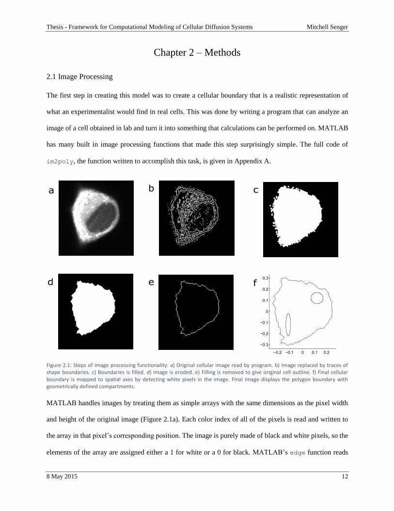
Figure 2.1: Steps of image processing functionality: a) Original cellular image read by program. b) Image
replaced by traces of shape boundaries. c) Boundaries is filled. d) Image is eroded. e) Filling is removed to
give original cell outline. f) Final cellular boundary is mapped to spatial axes by detecting white pixels in
the image. Final image displays the polygon boundary with geometrically defined compartments.
Figure 2.2 14
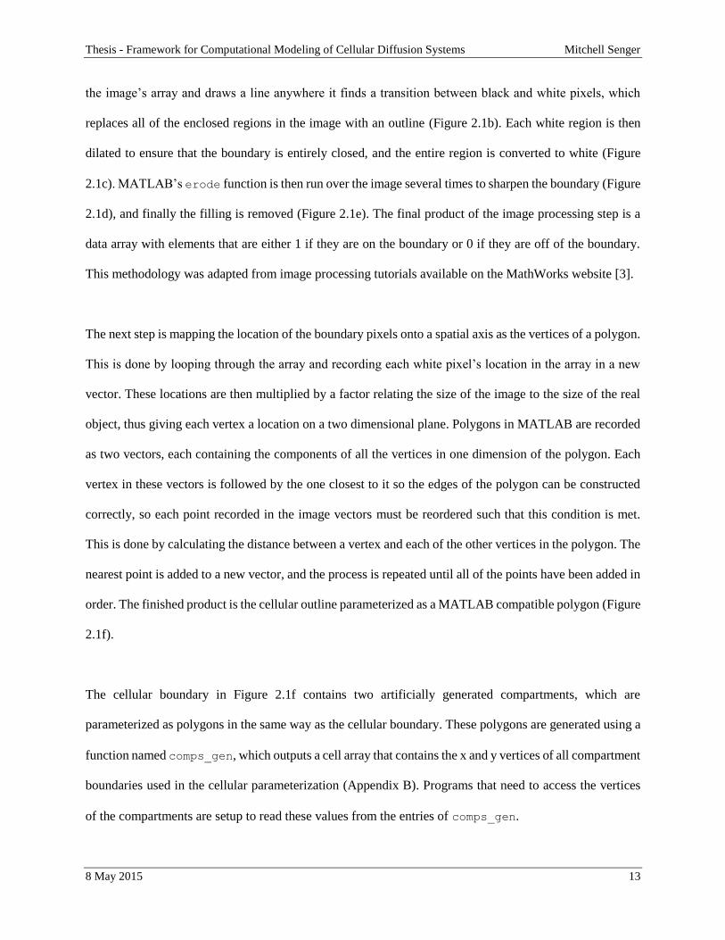
Grid is laid over boundary of cell and artificially generated compartments to discretize the region. a)
Evenly spaced points generated by the linspace function are laid over the space of the cell. b) Each set
of four adjacent points are treated as a box that contributes to the overall grid. The vertices of each
polygon are recorded in the data tracking array named gridinit.
Figure 2.3 15
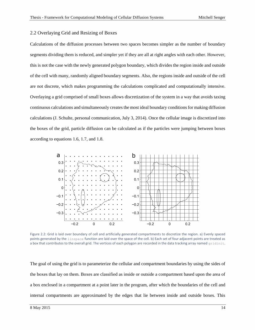
Comparison of the boundary portrayal for different uniform grid resolutions. Edges between boxes of two
different colors represent the grid’s approximation of the compartments drawn in white. a) 15 by 15 grid
producing a total of 225 boxes in the grid. Geometric resolution of the boundary via the grid is relatively
low. b) 50 by 50 grid producing a total of 2500 boxes in the grid. Representation of the boundary and
compartments via the grid is relatively accurate.
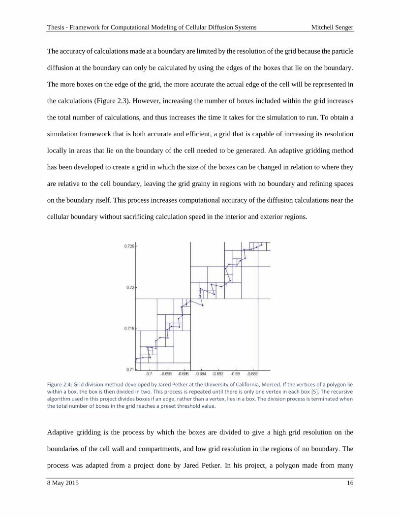
Figure 2.4 16
Grid division method developed by Jared Petker at the University of California, Merced. If the vertices of
a polygon lie within a box, the box is then divided in two. This process is repeated until there is only one
vertex in each box [5]. The recursive algorithm used in this project divides boxes if an edge, rather than a
vertex, lies in a box. The division process is terminated when the total number of boxes in the grid reaches
a preset threshold value.
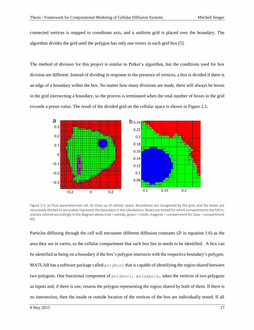
Figure 2.5 17
a) Final parameterized cell. b) Close up of cellular space. Boundaries are recognized by the grid, and the
boxes are recursively divided to accurately represent the boundary in the calculations. Boxes are tested for
which compartments the fall in, and are colored accordingly in the diagram above (red = outside, green =
inside, magenta = compartment #1, blue = compartment #2).
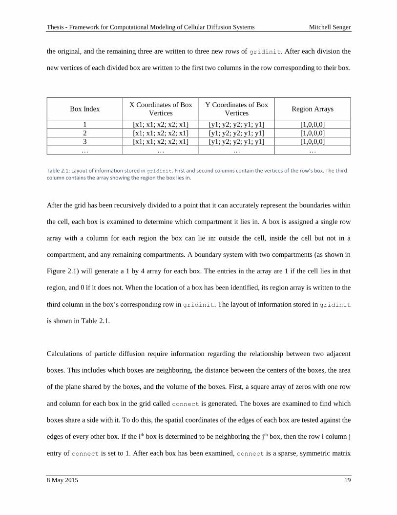
Table 2.1 19
Layout of information stored in gridinit. First and second columns contain the vertices of the row’s box.
The third column contains the array showing the region the box lies in.
Thesis - Framework for Computational Modeling of Cellular Diffusion Systems Mitchell Senger
8 May 2015 5
Figure 2.6 22
Code used for calculating flow of particles between boxes i and j. The code calculates the number of
particles moving between boxes, calculates the change in concentration for each box being examined, and
updates the array tracking the concentration of particles in each box. Every pair of neighboring boxes is
examined by looping through rows (index i) and columns (index j) of the connect array.
Figure 2.7 23
Code used to calculate the change in concentration due to the Fisher equation of logistic growth. This code
is used during each time step after the free diffusion of particles between all boxes have been calculated.
Figure 3.1 24
Plot of the particle concentration in a grid box with initial concentration of 50 nmol/μm3 in a system with
time steps that are too large. Because the time steps are too large, one box in the grid is calculated to have
a negative concentration at some time, and the concentration of every box in the grid diverges. At roughly
0.95 seconds, the cascade of concentration through the cell interrupts the calculations of the concentration
in the box plotted here, and the concentration diverges.
Figure 3.2 26
5E-9 nmol/μm3 concentration deposited in box with index 465 (cyan). b) Concentration of particles in the
box of initial deposit (cyan box in 3.2a, #465) over time for different diffusion coefficients. c) Concentration
of particles in a box near initial deposit (yellow box in 3.2a, #435) over time. d) Concentration of particles
in a box near initial deposit (magenta box in 3.2a, #464) over time. The concentration increases more
quickly than in 3.2c because of the shorter edge shared between this box and the initial deposit box. e)
Concentration of particles in a box far from initial deposit (black box in 3.2a, #227) over time. f)
Concentration of particles in a box in a cellular compartment far from initial deposit (white box in 3.2a,
#650) over time. The diffusion coefficient of the compartment was set to 3x that in the intracellular region,
so the concentration increases more quickly than the box plotted in 3.2e.
Figure 3.3 27
Contour plots of concentration over time for two separate simulations, one with the initial deposit located
in box 465 (cyan box in 3.2a), and one with the initial deposit located in box #650 (white box in 3.2a). a)
Box 465 origin at t = 0 seconds. b) Box 465 origin at t = 0.75 seconds. c) Box 465 origin at t = 1.5 seconds.
d) Box 650 origin at t = 0 seconds. e) Box 650 origin at t = 0.75 seconds. f) Box 650 origin at t = 1.5
seconds. Box #650’s concentration decreases more quickly than box #465’s because the diffusion
coefficient in the compartment was set to 3x that of the intracellular region, which allowed the particles to
reach the boundary of the compartment much faster. While the particles spread out more quickly in the
compartment origin simulation, the maximum concentration in the cell is always smaller than in the
intracellular origin simulation.
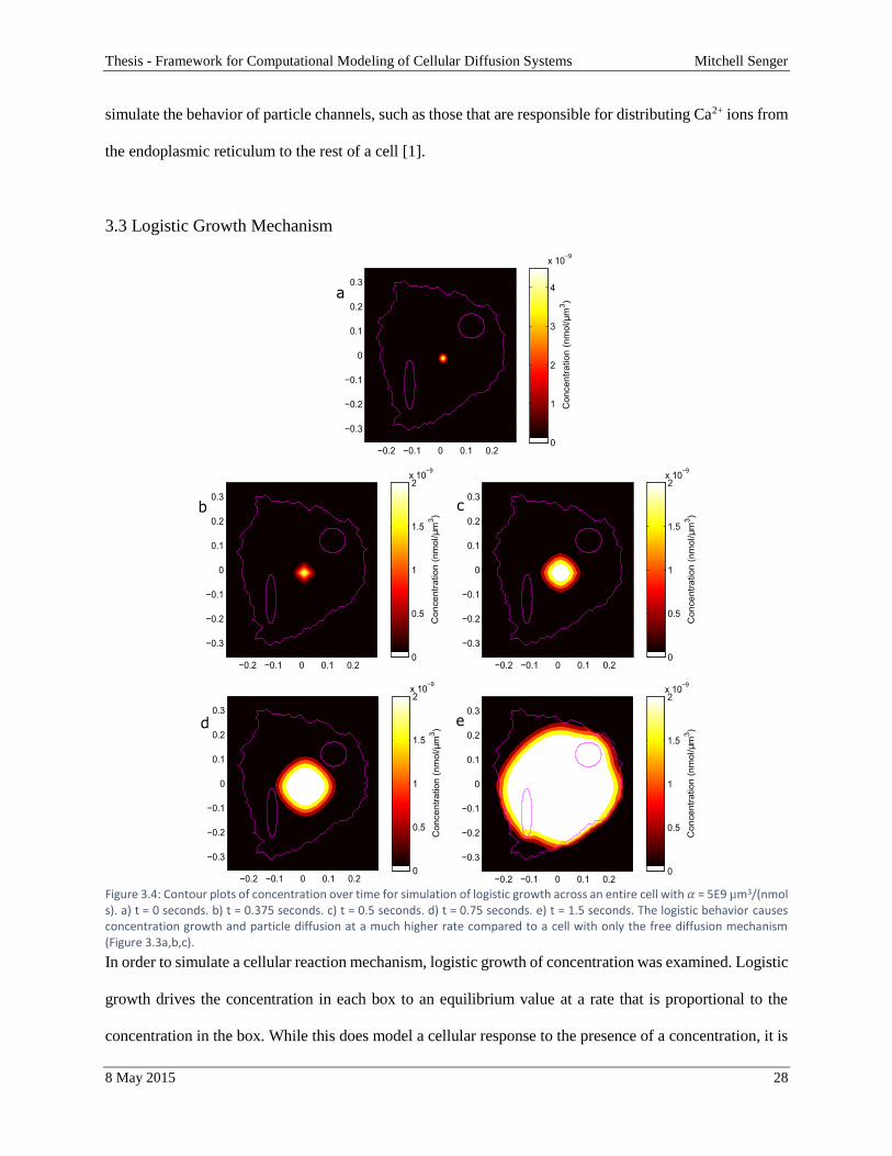
Figure 3.4 28
Contour plots of concentration over time for simulation of logistic growth across an entire cell with 𝛼 =
5E9 μm3/(nmol s). a) t = 0 seconds. b) t = 0.375 seconds. c) t = 0.5 seconds. d) t = 0.75 seconds. e) t = 1.5
Thesis - Framework for Computational Modeling of Cellular Diffusion Systems Mitchell Senger
8 May 2015 6
seconds. The logistic behavior causes concentration growth and particle diffusion at a much higher rate
compared to a cell with only the free diffusion mechanism (Figure 3.3a,b,c).
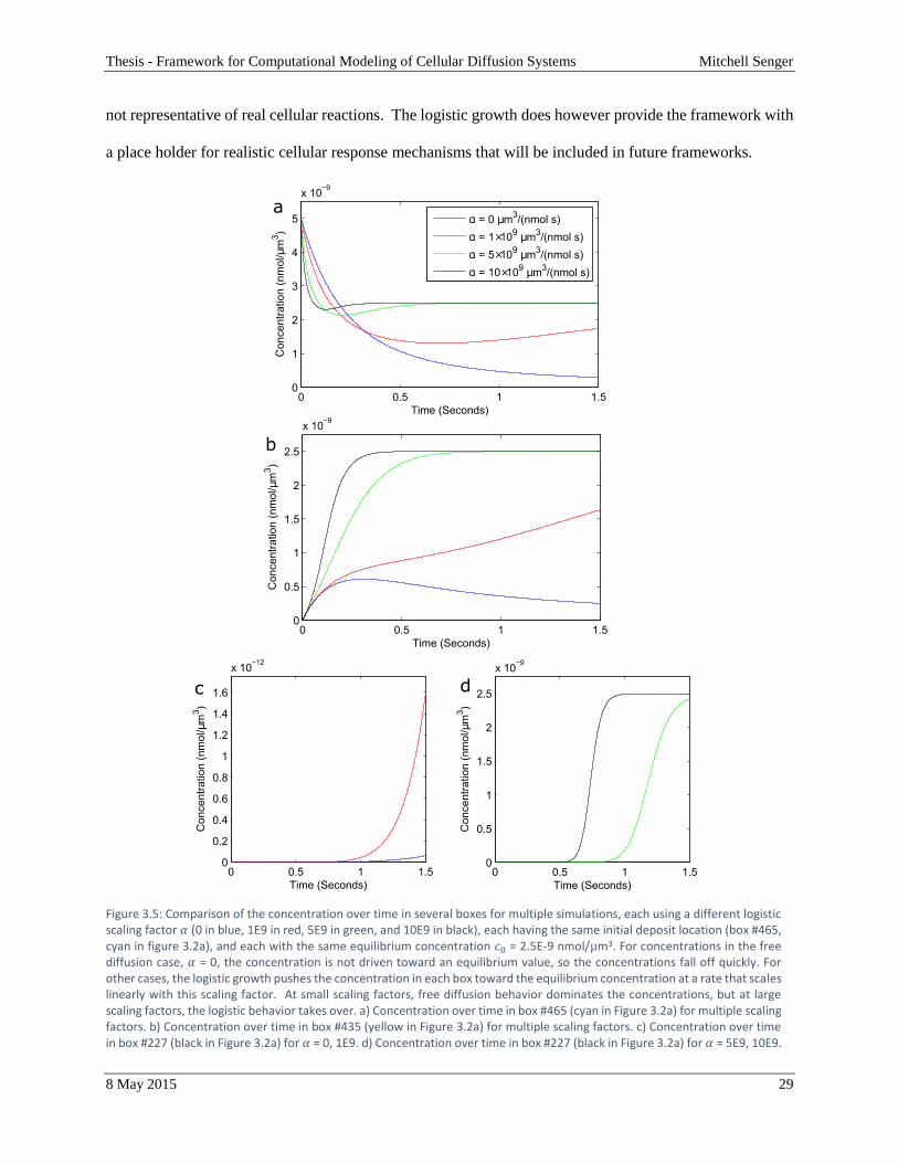
Figure 3.5 29
Comparison of the concentration over time in several boxes for multiple simulations, each using a different
logistic scaling factor 𝛼 (0 in blue, 1E9 in red, 5E9 in green, and 10E9 in black), each having the same
initial deposit location (box #465, cyan in figure 3.2a), and each with the same equilibrium concentration
𝑐0 = 2.5E-9 nmol/μm3. For concentrations in the free diffusion case, 𝛼 = 0, the concentration is not driven
toward an equilibrium value, so the concentrations fall off quickly. For other cases, the logistic growth
pushes the concentration in each box toward the equilibrium concentration at a rate that scales linearly with
this scaling factor. At small scaling factors, free diffusion behavior dominates the concentrations, but at
large scaling factors, the logistic behavior takes over. a) Concentration over time in box #465 (cyan in
Figure 3.2a) for multiple scaling factors. b) Concentration over time in box #435 (yellow in Figure 3.2a)
for multiple scaling factors. c) Concentration over time in box #227 (black in Figure 3.2a) for 𝛼 = 0, 1E9.
d) Concentration over time in box #227 (black in Figure 3.2a) for 𝛼 = 5E9, 10E9.
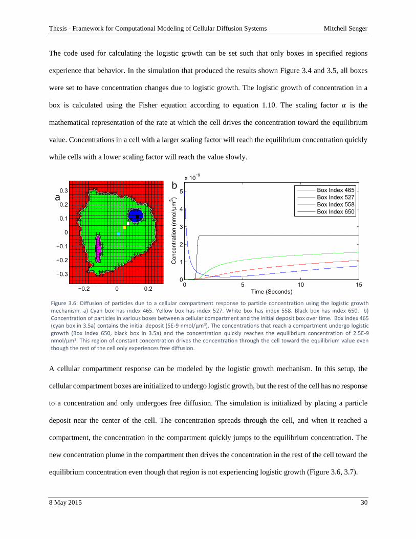
Figure 3.6 30
Diffusion of particles due to a cellular compartment response to particle concentration using the logistic
growth mechanism. a) Cyan box has index 465. Yellow box has index 527. White box has index 558. Black
box has index 650. b) Concentration of particles in various boxes between a cellular compartment and the
initial deposit box over time. Box index 465 (cyan box in 3.5a) contains the initial deposit (5E-9 nmol/μm3).
The concentrations that reach a compartment undergo logistic growth (Box index 650, black box in 3.5a)
and the concentration quickly reaches the equilibrium concentration of 2.5E-9 nmol/μm3. This region of
constant concentration drives the concentration through the cell toward the equilibrium value even though
the rest of the cell only experiences free diffusion.
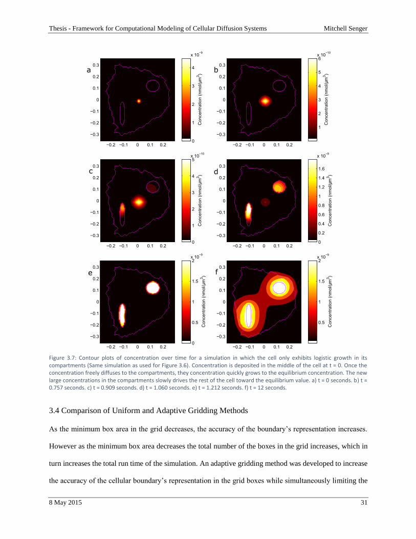
Figure 3.7 31
Contour plots of concentration over time for a simulation in which the cell only exhibits logistic growth in
its compartments (Same simulation as used for Figure 3.6). Concentration is deposited in the middle of the
cell at t = 0. Once the concentration freely diffuses to the compartments, they concentration quickly grows
to the equilibrium concentration. The new large concentrations in the compartments slowly drives the rest
of the cell toward the equilibrium value. a) t = 0 seconds. b) t = 0.757 seconds. c) t = 0.909 seconds. d) t =
1.060 seconds. e) t = 1.212 seconds. f) t = 12 seconds.
Figure 3.8 32
Plot of the simulation run time against the total number of boxes in the grid. Data was obtained from running
consecutive simulations with different box count thresholds. Trend line was fitted with R2 evaluated at
0.9999. The equation for the fitted line is given in equation 3.1.
Figure 3.9 33
Plot of the minimum box area against the number of boxes in the grid for the adaptive and uniform gridding
methods. Also plotted are the linear regressions of the adaptive grid and the uniform grid data; R2 for the
regressions are given by 0.992 and 1.000, respectively.
Thesis - Framework for Computational Modeling of Cellular Diffusion Systems Mitchell Senger
8 May 2015 7
Figure 4.1 35
Code used to automatically adjust the time steps used in calculations. If a negative concentration is detected,
then the variable switched is changed to 1, which triggers the reset code. After the time step has been
adjusted, the parameters are modified to meet the new time intervals and switched is then set back to 0.
The program begins looping again as normal.
Thesis - Framework for Computational Modeling of Cellular Diffusion Systems Mitchell Senger
8 May 2015 8
Chapter 1 – Introduction
1.1 Motivations
The process by which the actions of a cell or its components are influenced by its environment is a subject
of great interest in the field of biological physics. The variance of calcium ions in the cell is capable of
triggering responses from the cell or its constituent organelles, and therefore is one of the major factors in
signaling processes. This project developed a program that simulates the movement of intracellular
particles. A simulation system that can accurately model Ca2+ dynamics in a multicellular environment is a
powerful tool for biophysics research, and the program developed from this project will supply a framework
for such systems in the future.
1.2 Cellular Processes
The presence of certain ions act as a cellular signaling mechanism. One of the more interesting signaling
particles is the calcium ion (Ca2+), which is responsible for many physiological processes including nerve
action and cellular division [1]. These ions are regulated by the endoplasmic reticulum (ER) of a cell. Ca2+
is released from the ER when channels that are sensitive to secondary signaling molecules (namely IP3) are
stimulated to open [6]. The Ca2+ concentrations are subject to Brownian motion within the cell, but the
number of Ca2+ particles that are present in the first place is regulated by the ER.
Tang et al. from the Cornell Medical College demonstrated that the concentration of Ca2+ in a cell can
behave as an oscillatory system. At critical initial conditions, the concentration in the cell will be driven
towards an equilibrium concentration by the ER. Depending on the initial conditions, the concentration of
Ca2+ can oscillate around the equilibrium concentration [6].
The number of ions within a cell is regulated by the cell’s environment and the organelles within the cell,
but the motion of these intracellular ions is governed by Brownian motion. In order to develop a
Thesis - Framework for Computational Modeling of Cellular Diffusion Systems Mitchell Senger
8 May 2015 9
computational model where Ca2+ action can be modeled, a framework that is capable of simulating free
diffusion of particles within a cell was developed.
1.3 Modeling Overview
This project creates a deterministic computational model that accurately predicts the diffusion of particles
within a cell. This is done using gridding methods to calculate the diffusion of particles from an initial
deposit between the boxes of that grid. The model is capable of analyzing an image of a cell and
parameterizing a boundary based upon that image. The space of the cell is discretized by overlaying the
cell with an adaptive grid that can recursively form to the presence of a boundary. Calculations of free
diffusion are then performed between boxes of the grid, and the concentration in each box is recorded over
a period of time. Several computational functions that are capable of reading the recorded data and
displaying it in a useful manner have also been created.
1.4 Premise for Calculations
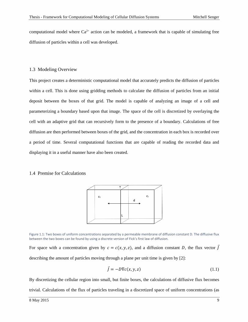
Figure 1.1: Two boxes of uniform concentrations separated by a permeable membrane of diffusion constant D. The diffusive flux between the two boxes can be found by using a discrete version of Fick’s first law of diffusion.
For space with a concentration given by 𝑐 = 𝑐(𝑥, 𝑦, 𝑧), and a diffusion constant 𝐷, the flux vector 𝐽
describing the amount of particles moving through a plane per unit time is given by [2]:
𝐽 = −𝐷∇𝑐(𝑥, 𝑦, 𝑧) (1.1)
By discretizing the cellular region into small, but finite boxes, the calculations of diffusive flux becomes
trivial. Calculations of the flux of particles traveling in a discretized space of uniform concentrations (as
Thesis - Framework for Computational Modeling of Cellular Diffusion Systems Mitchell Senger
8 May 2015 10
shown in Figure 1.1) only requires the magnitude of the flux and allows for the discretization of the gradient
used in equation 1.1.
𝐽 = −𝐷∆𝑐
∆𝑟 (1.2)
Fick’s first law of diffusion gives a method for calculating the diffusive flux through a plane from the
concentration of particles on either side of the plane. The number of particles 𝑁 passing through a plane of
area 𝐴 per time is given by:
∆𝑁
∆𝑡= 𝐽 ∙ 𝐴 (1.3)
For the discretizes space shown in Figure 1.1, the plane between the boxes has side lengths 𝐿 and 𝑇. Since
the concentration in each box is uniform, the flux vector is always parallel with the area vector of the plane.
Therefore equation 1.3 can be simplified to the following:
∆𝑁
∆𝑡= 𝐽𝐿𝑇 (1.4)
Inserting equation 1.2 for the flux magnitude 𝐽 gives:
∆𝑁
∆𝑡= −𝐷
∆𝑐
∆𝑟𝐿𝑇 (1.5)
The uniform concentrations on either side of the plane are given by 𝑐1 and 𝑐2, and the average distance
between points in either box is 𝑑. The number of particles moving between boxes in a given time ∆𝑡 is
given by:
Δ𝑁 = 𝐷(𝑐1 − 𝑐2 )𝐿𝑇Δ𝑡/𝑑 (1.6)
The new concentrations in the original boxes after time of diffusion ∆𝑡 is then given by:
𝑐1′ = 𝑐1 − Δ𝑁/𝑉1 (1.7)
𝑐2′ = 𝑐2 + Δ𝑁/𝑉2 (1.8)
After overlaying an appropriate grid on the space of a cell, this model uses equations 1.6, 1.7, and 1.8 to
calculate the flow are particles through the cell by calculating the diffusive flux between every neighboring
box within the grid.
Thesis - Framework for Computational Modeling of Cellular Diffusion Systems Mitchell Senger
8 May 2015 11
The concentration of particles may also be influenced by the amount of particles that occupy the cell. This
project uses logistic growth to simulate a cellular reaction based on the concentration of particles in the cell.
Logistic growth or decay drives the concentration in each region to an equilibrium value. The rate of growth
or decay increases as the difference between the current concentration and the equilibrium concentration
increases, and vice versa. The change of concentration in a region per unit time due to this logistic behavior
can be modeled by the Fisher equation [4], shown in equation 1.9.
𝜕𝑐
𝜕𝑡= 𝛼(𝑐0𝑐 − 𝑐2) (1.9)
In equation 1.9, 𝛼 scales the cell’s response to the concentration, 𝑐 is the concentration of the region of
interest, and 𝑐0 is the equilibrium concentration that the logistic behavior drives the concentration to. The
model uses the discretized version of equation 1.9 (equation 1.10) to simulate the cell responding the
presence of particles within different regions.
∆𝑐 = 𝛼Δ𝑡(𝑐0𝑐 − 𝑐2) (1.10)
Thesis - Framework for Computational Modeling of Cellular Diffusion Systems Mitchell Senger
8 May 2015 12
Chapter 2 – Methods
2.1 Image Processing
The first step in creating this model was to create a cellular boundary that is a realistic representation of
what an experimentalist would find in real cells. This was done by writing a program that can analyze an
image of a cell obtained in lab and turn it into something that calculations can be performed on. MATLAB
has many built in image processing functions that made this step surprisingly simple. The full code of
im2poly, the function written to accomplish this task, is given in Appendix A.
MATLAB handles images by treating them as simple arrays with the same dimensions as the pixel width
and height of the original image (Figure 2.1a). Each color index of all of the pixels is read and written to
the array in that pixel’s corresponding position. The image is purely made of black and white pixels, so the
elements of the array are assigned either a 1 for white or a 0 for black. MATLAB’s edge function reads
Figure 2.1: Steps of image processing functionality: a) Original cellular image read by program. b) Image replaced by traces of shape boundaries. c) Boundaries is filled. d) Image is eroded. e) Filling is removed to give original cell outline. f) Final cellular boundary is mapped to spatial axes by detecting white pixels in the image. Final image displays the polygon boundary with geometrically defined compartments.
Thesis - Framework for Computational Modeling of Cellular Diffusion Systems Mitchell Senger
8 May 2015 13
the image’s array and draws a line anywhere it finds a transition between black and white pixels, which
replaces all of the enclosed regions in the image with an outline (Figure 2.1b). Each white region is then
dilated to ensure that the boundary is entirely closed, and the entire region is converted to white (Figure
2.1c). MATLAB’s erode function is then run over the image several times to sharpen the boundary (Figure
2.1d), and finally the filling is removed (Figure 2.1e). The final product of the image processing step is a
data array with elements that are either 1 if they are on the boundary or 0 if they are off of the boundary.
This methodology was adapted from image processing tutorials available on the MathWorks website [3].
The next step is mapping the location of the boundary pixels onto a spatial axis as the vertices of a polygon.
This is done by looping through the array and recording each white pixel’s location in the array in a new
vector. These locations are then multiplied by a factor relating the size of the image to the size of the real
object, thus giving each vertex a location on a two dimensional plane. Polygons in MATLAB are recorded
as two vectors, each containing the components of all the vertices in one dimension of the polygon. Each
vertex in these vectors is followed by the one closest to it so the edges of the polygon can be constructed
correctly, so each point recorded in the image vectors must be reordered such that this condition is met.
This is done by calculating the distance between a vertex and each of the other vertices in the polygon. The
nearest point is added to a new vector, and the process is repeated until all of the points have been added in
order. The finished product is the cellular outline parameterized as a MATLAB compatible polygon (Figure
2.1f).
The cellular boundary in Figure 2.1f contains two artificially generated compartments, which are
parameterized as polygons in the same way as the cellular boundary. These polygons are generated using a
function named comps_gen, which outputs a cell array that contains the x and y vertices of all compartment
boundaries used in the cellular parameterization (Appendix B). Programs that need to access the vertices
of the compartments are setup to read these values from the entries of comps_gen.
Thesis - Framework for Computational Modeling of Cellular Diffusion Systems Mitchell Senger
8 May 2015 14
2.2 Overlaying Grid and Resizing of Boxes
Calculations of the diffusion processes between two spaces becomes simpler as the number of boundary
segments dividing them is reduced, and simpler yet if they are all at right angles with each other. However,
this is not the case with the newly generated polygon boundary, which divides the region inside and outside
of the cell with many, randomly aligned boundary segments. Also, the regions inside and outside of the cell
are not discrete, which makes programming the calculations complicated and computationally intensive.
Overlaying a grid comprised of small boxes allows discretization of the system in a way that avoids taxing
continuous calculations and simultaneously creates the most ideal boundary conditions for making diffusion
calculations (J. Schulte, personal communication, July 3, 2014). Once the cellular image is discretized into
the boxes of the grid, particle diffusion can be calculated as if the particles were jumping between boxes
according to equations 1.6, 1.7, and 1.8.
The goal of using the grid is to parameterize the cellular and compartment boundaries by using the sides of
the boxes that lay on them. Boxes are classified as inside or outside a compartment based upon the area of
a box enclosed in a compartment at a point later in the program, after which the boundaries of the cell and
internal compartments are approximated by the edges that lie between inside and outside boxes. This
Figure 2.2: Grid is laid over boundary of cell and artificially generated compartments to discretize the region. a) Evenly spaced points generated by the linspace function are laid over the space of the cell. b) Each set of four adjacent points are treated as a box that contributes to the overall grid. The vertices of each polygon are recorded in the data tracking array named gridinit.
Thesis - Framework for Computational Modeling of Cellular Diffusion Systems Mitchell Senger
8 May 2015 15
approximation allows for the use of equations 1.6, 1.7, and 1.8 in calculations of diffusion across boundaries
in the region.
This process is started by generating evenly spaced points across the cell using the linspace function
(Figure 2.2a). Each of these points is treated as the bottom left point of a box with vertical and horizontal
side lengths equal to the distance between vertical points and horizontal points, respectively. Each adjacent
set of four points make the vertices of one box in the grid. Since the number of boxes is determined by the
number of points laid over the space, the number of points in the horizontal and vertical directions
determines the resolution of the spatial discretization. Each box is assigned a number index, and the vertices
of each box are recorded as a polygon in a cell array called gridinit. The significance of this array is
discussed in section 2.3.
Figure 2.3: Comparison of the boundary portrayal for different uniform grid resolutions. Edges between boxes of two different colors represent the grid’s approximation of the compartments drawn in white. a) 15 by 15 grid producing a total of 225 boxes in the grid. Geometric resolution of the boundary via the grid is relatively low. b) 50 by 50 grid producing a total of 2500 boxes in the grid. Representation of the boundary and compartments via the grid is relatively accurate.
Thesis - Framework for Computational Modeling of Cellular Diffusion Systems Mitchell Senger
8 May 2015 16
The accuracy of calculations made at a boundary are limited by the resolution of the grid because the particle
diffusion at the boundary can only be calculated by using the edges of the boxes that lie on the boundary.
The more boxes on the edge of the grid, the more accurate the actual edge of the cell will be represented in
the calculations (Figure 2.3). However, increasing the number of boxes included within the grid increases
the total number of calculations, and thus increases the time it takes for the simulation to run. To obtain a
simulation framework that is both accurate and efficient, a grid that is capable of increasing its resolution
locally in areas that lie on the boundary of the cell needed to be generated. An adaptive gridding method
has been developed to create a grid in which the size of the boxes can be changed in relation to where they
are relative to the cell boundary, leaving the grid grainy in regions with no boundary and refining spaces
on the boundary itself. This process increases computational accuracy of the diffusion calculations near the
cellular boundary without sacrificing calculation speed in the interior and exterior regions.
Adaptive gridding is the process by which the boxes are divided to give a high grid resolution on the
boundaries of the cell wall and compartments, and low grid resolution in the regions of no boundary. The
process was adapted from a project done by Jared Petker. In his project, a polygon made from many
Figure 2.4: Grid division method developed by Jared Petker at the University of California, Merced. If the vertices of a polygon lie within a box, the box is then divided in two. This process is repeated until there is only one vertex in each box [5]. The recursive algorithm used in this project divides boxes if an edge, rather than a vertex, lies in a box. The division process is terminated when the total number of boxes in the grid reaches a preset threshold value.
Thesis - Framework for Computational Modeling of Cellular Diffusion Systems Mitchell Senger
8 May 2015 17
connected vertices is mapped to coordinate axis, and a uniform grid is placed over the boundary. The
algorithm divides the grid until the polygon has only one vertex in each grid box [5].
The method of division for this project is similar to Petker’s algorithm, but the conditions used for box
division are different. Instead of dividing in response to the presence of vertices, a box is divided if there is
an edge of a boundary within the box. No matter how many divisions are made, there will always be boxes
in the grid intersecting a boundary, so the process is terminated when the total number of boxes in the grid
exceeds a preset value. The result of the divided grid on the cellular space is shown in Figure 2.5.
Particles diffusing through the cell will encounter different diffusion constants (𝐷 in equation 1.6) as the
area they are in varies, so the cellular compartment that each box lies in needs to be identified. A box can
be identified as being on a boundary if the box’s polygon intersects with the respective boundary’s polygon.
MATLAB has a software package called polybool that is capable of identifying the region shared between
two polygons. One functional component of polybool, polyxpoly, takes the vertices of two polygons
as inputs and, if there is one, returns the polygon representing the region shared by both of them. If there is
no intersection, then the inside or outside location of the vertices of the box are individually tested. If all
Figure 2.5: a) Final parameterized cell. b) Close up of cellular space. Boundaries are recognized by the grid, and the boxes are recursively divided to accurately represent the boundary in the calculations. Boxes are tested for which compartments the fall in, and are colored accordingly in the diagram above (red = outside, green = inside, magenta = compartment #1, blue = compartment #2).
0.1 0.15 0.2
0.08
0.1
0.12
0.14
0.16
0.18
0.2
0.22
0.24b
Thesis - Framework for Computational Modeling of Cellular Diffusion Systems Mitchell Senger
8 May 2015 18
vertices are inside the boundary, then the box is marked as inside the boundary, and vice versa. If there is
an intersection, then the box is marked as being on the boundary. The area of the box enclosed within the
boundary is compared to the area of the box outside of the boundary. If the area inside is greater than the
outside then the box as a whole is reclassified as an inside box, and vice versa. By doing this, diffusion
across the cell boundary can be calculated by using the edges of the boxes that make up the border between
inside and outside boxes. The result of the box classification process is shown by the box colors in Figure
2.5.
Particles traveling inside the cell will travel faster than those moving through the boundary because the
diffusion coefficient of the intracellular region is larger than that of the cellular boundary. The grid laid
over the region also presents a convenient way to govern the diffusion rates of particles moving through
the cell. Diffusion constants can be assigned to each edge of each box in the grid to govern the speed at
which particles are allowed to move between them. The regions inside and outside of the cell and the
different compartments inside of the cell will have different diffusion rates and will react differently to the
presence of particles within space of interest based on the biology of the cell and its environment. The boxes
within the specific regions are programmed with properties that reflect the regions that they lie in. Arrays
that track the properties associated with the boxes are generated at this point in the code so that when
particle flow calculations are performed, the properties of the two considered boxes are readily accessible.
2.3 Property Tracking
An array, referred to as gridinit (previously mentioned in section 2.2), that has a length equal to the total
number of boxes in the grid is created, and each box is assigned to a row within this array. The array is used
to track information regarding the geometric location of each box and the compartment that the box lies in.
When the uniform grid is initially laid over the cell, the spatial coordinates of each box are stored in the
first two columns. If a box if divided during recursion, then one of the new boxes is left in the same row as
Thesis - Framework for Computational Modeling of Cellular Diffusion Systems Mitchell Senger
8 May 2015 19
the original, and the remaining three are written to three new rows of gridinit. After each division the
new vertices of each divided box are written to the first two columns in the row corresponding to their box.
Table 2.1: Layout of information stored in gridinit. First and second columns contain the vertices of the row’s box. The third column contains the array showing the region the box lies in.
After the grid has been recursively divided to a point that it can accurately represent the boundaries within
the cell, each box is examined to determine which compartment it lies in. A box is assigned a single row
array with a column for each region the box can lie in: outside the cell, inside the cell but not in a
compartment, and any remaining compartments. A boundary system with two compartments (as shown in
Figure 2.1) will generate a 1 by 4 array for each box. The entries in the array are 1 if the cell lies in that
region, and 0 if it does not. When the location of a box has been identified, its region array is written to the
third column in the box’s corresponding row in gridinit. The layout of information stored in gridinit
is shown in Table 2.1.
Calculations of particle diffusion require information regarding the relationship between two adjacent
boxes. This includes which boxes are neighboring, the distance between the centers of the boxes, the area
of the plane shared by the boxes, and the volume of the boxes. First, a square array of zeros with one row
and column for each box in the grid called connect is generated. The boxes are examined to find which
boxes share a side with it. To do this, the spatial coordinates of the edges of each box are tested against the
edges of every other box. If the ith box is determined to be neighboring the jth box, then the row i column j
entry of connect is set to 1. After each box has been examined, connect is a sparse, symmetric matrix
Box Index X Coordinates of Box
Vertices
Y Coordinates of Box
Vertices Region Arrays
1 [x1; x1; x2; x2; x1] [y1; y2; y2; y1; y1] [1,0,0,0]
2 [x1; x1; x2; x2; x1] [y1; y2; y2; y1; y1] [1,0,0,0]
3 [x1; x1; x2; x2; x1] [y1; y2; y2; y1; y1] [1,0,0,0]
… … … …
Thesis - Framework for Computational Modeling of Cellular Diffusion Systems Mitchell Senger
8 May 2015 20
populated with ones at entries that have the indices of two boxes are neighboring and zeros everywhere
else.
Other data needed for calculations is also stored in the same matrix format. If two boxes are found to share
an edge, then the center point of each box is computed and the distance between the two center points is
found. This distance is stored in a new sparse matrix called distances in the same format as the
information stored in connect, except instead of ones, the matrix is populated with the distances between
the two boxes. Another matrix, called edges, is constructed in much the same way as distances, but it
is populated with the length of the edge shared by the two boxes. A column matrix named areas that has
length equal to the number of boxes in the grid is constructed. The array is populated with the areas of the
face of each box. The thickness of the cell is also set, and combining this information with the box face
areas allows for the quick calculation of the volume of each box.
Lastly, the diffusion coefficients are assigned to the planes that lie between boxes. The program uses
connect to determine which boxes are neighboring, and assigns a diffusion coefficient to the face that the
boxes share if they are neighboring. Faces that lie between boxes that are in the same compartment are
assigned a diffusion coefficient that is specific to that compartment. Faces between boxes that lie in different
cellular regions are assigned a separate coefficient that represents the “leakage” rate of particles moving
from one compartment to another. A matrix named coeffs holds the diffusion coefficient of each
neighboring pair in the grid.
Together, distances, coeffs, edges, areas, connect, and gridinit hold all of the information
needed to calculate the diffusive flux between each box in the grid with equations 1.6, 1.7, and 1.8. The
symmetric matrix format of distances, coeffs, edges, and connect presents a convenient method for
data storage as well as the rapid recovery of data needed for calculations later on. A full copy of the code
used to generate the grid and the matrices used in calculations is given in Appendix C.
Thesis - Framework for Computational Modeling of Cellular Diffusion Systems Mitchell Senger
8 May 2015 21
2.4 Calculations of Particle Flow
At this point the program is given a start time and end time as well as the time steps taken between the two,
and the flow of particles is calculated throughout the cell with these time constraints. The user specifies the
box in which some initial particle concentration will be deposited, and the flow of particles through the cell
is calculated based on this deposit. Two column arrays are generated to record the concentration of particles
in each box over for each time step. The first, named con_before, holds the concentrations of particles in
each box at the beginning of each time step and is not updated until all calculations have been completed
for the time step. The second, con_after, holds the concentration of particles in each box during each
time step and is continuously updated through each time step.
During each time step, the entries of connect are searched to find which boxes are neighboring. Because
connect is a symmetric matrix, only the upper half is searched. This is done by using two for loops, one
cycling through the rows and one cycling through the columns. When calculations of particle diffusion are
performed, the value of the concentrations of the boxes of interest are pulled from con_before, and the
change in concentrations for both boxes are recorded in con_after. The diffusion constant of the pair of
boxes is pulled from coeffs by calling the entry that has indices that correspond to the two boxes of
interest. The length of the edge shared between the boxes and the distance between the center points of the
boxes are pulled from edges and distances in the same way. The areas of the faces of the two boxes are
pulled from areas at this time as well. The number of particles moving between every pair of neighboring
boxes is calculated using equation 1.6, and the change in concentrations for each box are calculated using
equations 1.7 and 1.8. The flow of particles is calculated for all boxes before con_before is updated with
the new concentrations so the order in which they are examined does not affect the outcome of the
calculations. Figure 2.6 shows the code used to conduct the calculations.
In addition to the free diffusion calculations, the cell’s reaction to the presence of particles needs to be
examined. This model calculates logistic growth as a place holder for the more complex reaction behavior
Thesis - Framework for Computational Modeling of Cellular Diffusion Systems Mitchell Senger
8 May 2015 22
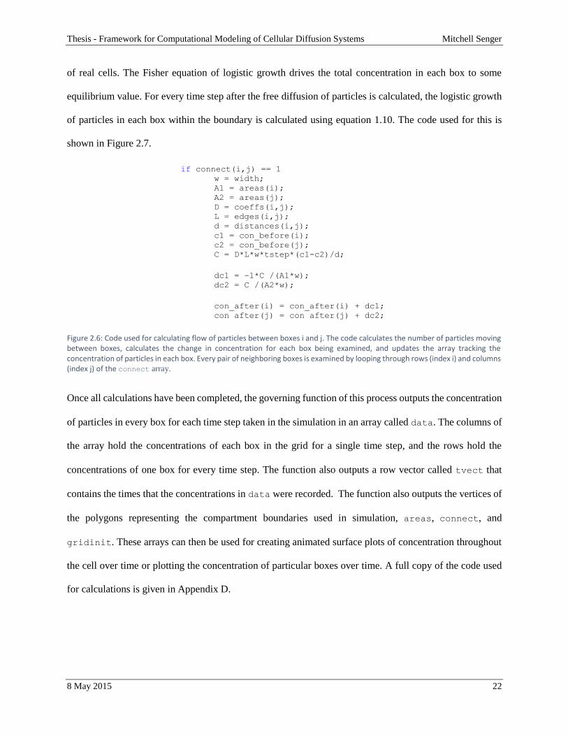
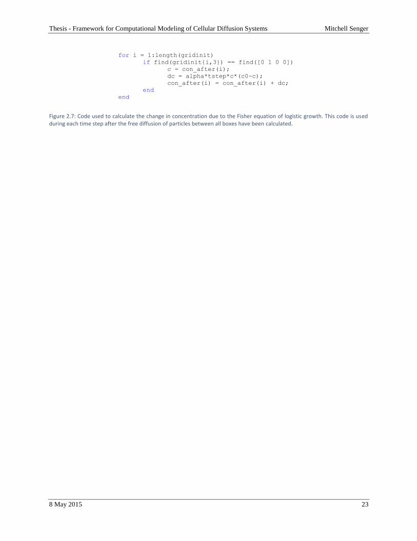
of real cells. The Fisher equation of logistic growth drives the total concentration in each box to some
equilibrium value. For every time step after the free diffusion of particles is calculated, the logistic growth
of particles in each box within the boundary is calculated using equation 1.10. The code used for this is
shown in Figure 2.7.
Once all calculations have been completed, the governing function of this process outputs the concentration
of particles in every box for each time step taken in the simulation in an array called data. The columns of
the array hold the concentrations of each box in the grid for a single time step, and the rows hold the
concentrations of one box for every time step. The function also outputs a row vector called tvect that
contains the times that the concentrations in data were recorded. The function also outputs the vertices of
the polygons representing the compartment boundaries used in simulation, areas, connect, and
gridinit. These arrays can then be used for creating animated surface plots of concentration throughout
the cell over time or plotting the concentration of particular boxes over time. A full copy of the code used
for calculations is given in Appendix D.
if connect(i,j) == 1 w = width; A1 = areas(i); A2 = areas(j); D = coeffs(i,j); L = edges(i,j); d = distances(i,j);
c1 = con_before(i); c2 = con_before(j); C = D*L*w*tstep*(c1-c2)/d;
dc1 = -1*C /(A1*w); dc2 = C /(A2*w);
con_after(i) = con_after(i) + dc1; con_after(j) = con_after(j) + dc2;
Figure 2.6: Code used for calculating flow of particles between boxes i and j. The code calculates the number of particles moving between boxes, calculates the change in concentration for each box being examined, and updates the array tracking the concentration of particles in each box. Every pair of neighboring boxes is examined by looping through rows (index i) and columns (index j) of the connect array.
Thesis - Framework for Computational Modeling of Cellular Diffusion Systems Mitchell Senger
8 May 2015 23
for i = 1:length(gridinit) if find(gridinit{i,3}) == find([0 1 0 0])
c = con_after(i); dc = alpha*tstep*c*(c0-c); con_after(i) = con_after(i) + dc;
end end
Figure 2.7: Code used to calculate the change in concentration due to the Fisher equation of logistic growth. This code is used during each time step after the free diffusion of particles between all boxes have been calculated.
Thesis - Framework for Computational Modeling of Cellular Diffusion Systems Mitchell Senger
8 May 2015 24
Chapter 3 – Results
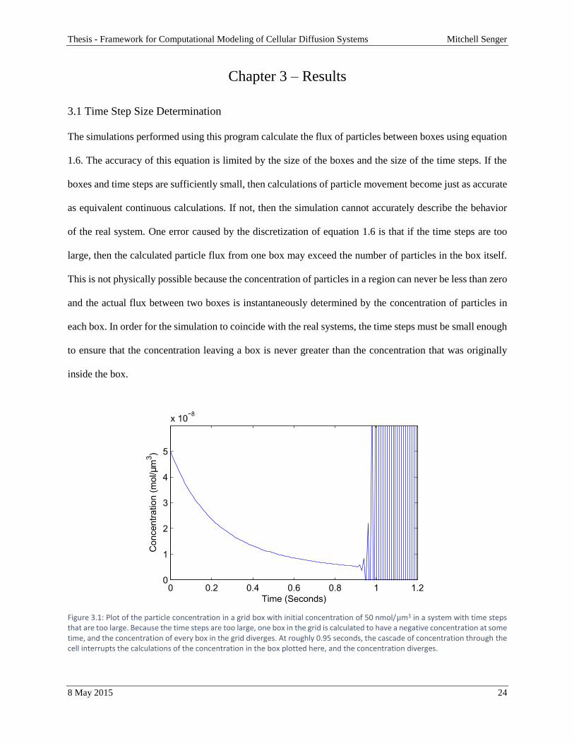
3.1 Time Step Size Determination
The simulations performed using this program calculate the flux of particles between boxes using equation
1.6. The accuracy of this equation is limited by the size of the boxes and the size of the time steps. If the
boxes and time steps are sufficiently small, then calculations of particle movement become just as accurate
as equivalent continuous calculations. If not, then the simulation cannot accurately describe the behavior
of the real system. One error caused by the discretization of equation 1.6 is that if the time steps are too
large, then the calculated particle flux from one box may exceed the number of particles in the box itself.
This is not physically possible because the concentration of particles in a region can never be less than zero
and the actual flux between two boxes is instantaneously determined by the concentration of particles in
each box. In order for the simulation to coincide with the real systems, the time steps must be small enough
to ensure that the concentration leaving a box is never greater than the concentration that was originally
inside the box.
Figure 3.1: Plot of the particle concentration in a grid box with initial concentration of 50 nmol/µm3 in a system with time steps that are too large. Because the time steps are too large, one box in the grid is calculated to have a negative concentration at some time, and the concentration of every box in the grid diverges. At roughly 0.95 seconds, the cascade of concentration through the cell interrupts the calculations of the concentration in the box plotted here, and the concentration diverges.
Thesis - Framework for Computational Modeling of Cellular Diffusion Systems Mitchell Senger
8 May 2015 25
If the number of particles leaving a box is calculated to be larger than the number of particles in the box,
then the resultant concentration in the box will become negative. Future calculations in boxes neighboring
a box with negative concentration find that particle diffusion will occur even without the presence of
particles in the region. Setting the time steps too large creates a cascading effect in the concentration
throughout the cell which causes divergence of the concentration of particles in all boxes over time. This
behavior can be recognized by observation of the divergent behavior in a plot of a box’s concentration as
time progresses (Figure 3.1). The solution to this error is selecting a sufficiently small time step such that
the calculated particle flux between two boxes coincides with continuous time.
3.2 Free Diffusion Mechanism
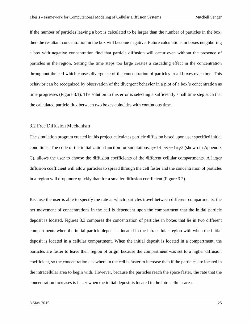
The simulation program created in this project calculates particle diffusion based upon user specified initial
conditions. The code of the initialization function for simulations, grid_overlay2 (shown in Appendix
C), allows the user to choose the diffusion coefficients of the different cellular compartments. A larger
diffusion coefficient will allow particles to spread through the cell faster and the concentration of particles
in a region will drop more quickly than for a smaller diffusion coefficient (Figure 3.2).
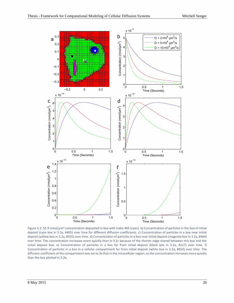
Because the user is able to specify the rate at which particles travel between different compartments, the
net movement of concentrations in the cell is dependent upon the compartment that the initial particle
deposit is located. Figures 3.3 compares the concentration of particles in boxes that lie in two different
compartments when the initial particle deposit is located in the intracellular region with when the initial
deposit is located in a cellular compartment. When the initial deposit is located in a compartment, the
particles are faster to leave their region of origin because the compartment was set to a higher diffusion
coefficient, so the concentration elsewhere in the cell is faster to increase than if the particles are located in
the intracellular area to begin with. However, because the particles reach the space faster, the rate that the
concentration increases is faster when the initial deposit is located in the intracellular area.
Thesis - Framework for Computational Modeling of Cellular Diffusion Systems Mitchell Senger
8 May 2015 26
Figure 3.2: 5E-9 nmol/µm3 concentration deposited in box with index 465 (cyan). b) Concentration of particles in the box of initial deposit (cyan box in 3.2a, #465) over time for different diffusion coefficients. c) Concentration of particles in a box near initial deposit (yellow box in 3.2a, #435) over time. d) Concentration of particles in a box near initial deposit (magenta box in 3.2a, #464) over time. The concentration increases more quickly than in 3.2c because of the shorter edge shared between this box and the initial deposit box. e) Concentration of particles in a box far from initial deposit (black box in 3.2a, #227) over time. f) Concentration of particles in a box in a cellular compartment far from initial deposit (white box in 3.2a, #650) over time. The diffusion coefficient of the compartment was set to 3x that in the intracellular region, so the concentration increases more quickly than the box plotted in 3.2e.
Thesis - Framework for Computational Modeling of Cellular Diffusion Systems Mitchell Senger
8 May 2015 27
The adaptability of the diffusion coefficient assignment process may provide another useful feature to the
simulation. Assigning a leakage coefficient of zero to every cell interface apart from a select few will cause
the particles to enter or exit a compartment from only a few points. This behavior could be adapted to
Figure 3.3: Contour plots of concentration over time for two separate simulations, one with the initial deposit located in box 465 (cyan box in 3.2a), and one with the initial deposit located in box #650 (white box in 3.2a). a) Box 465 origin at t = 0 seconds. b) Box 465 origin at t = 0.75 seconds. c) Box 465 origin at t = 1.5 seconds. d) Box 650 origin at t = 0 seconds. e) Box 650 origin at t = 0.75 seconds. f) Box 650 origin at t = 1.5 seconds. Box #650’s concentration decreases more quickly than box #465’s because the diffusion coefficient in the compartment was set to 3x that of the intracellular region, which allowed the particles to reach the boundary of the compartment much faster. While the particles spread out more quickly in the compartment origin simulation, the maximum concentration in the cell is always smaller than in the intracellular origin simulation.
Thesis - Framework for Computational Modeling of Cellular Diffusion Systems Mitchell Senger
8 May 2015 28
simulate the behavior of particle channels, such as those that are responsible for distributing Ca2+ ions from
the endoplasmic reticulum to the rest of a cell [1].
3.3 Logistic Growth Mechanism
In order to simulate a cellular reaction mechanism, logistic growth of concentration was examined. Logistic
growth drives the concentration in each box to an equilibrium value at a rate that is proportional to the
concentration in the box. While this does model a cellular response to the presence of a concentration, it is
Figure 3.4: Contour plots of concentration over time for simulation of logistic growth across an entire cell with 𝛼 = 5E9 µm3/(nmol s). a) t = 0 seconds. b) t = 0.375 seconds. c) t = 0.5 seconds. d) t = 0.75 seconds. e) t = 1.5 seconds. The logistic behavior causes concentration growth and particle diffusion at a much higher rate compared to a cell with only the free diffusion mechanism (Figure 3.3a,b,c).
Thesis - Framework for Computational Modeling of Cellular Diffusion Systems Mitchell Senger
8 May 2015 29
not representative of real cellular reactions. The logistic growth does however provide the framework with
a place holder for realistic cellular response mechanisms that will be included in future frameworks.
Figure 3.5: Comparison of the concentration over time in several boxes for multiple simulations, each using a different logistic scaling factor 𝛼 (0 in blue, 1E9 in red, 5E9 in green, and 10E9 in black), each having the same initial deposit location (box #465, cyan in figure 3.2a), and each with the same equilibrium concentration 𝑐0 = 2.5E-9 nmol/µm3. For concentrations in the free diffusion case, 𝛼 = 0, the concentration is not driven toward an equilibrium value, so the concentrations fall off quickly. For other cases, the logistic growth pushes the concentration in each box toward the equilibrium concentration at a rate that scales linearly with this scaling factor. At small scaling factors, free diffusion behavior dominates the concentrations, but at large scaling factors, the logistic behavior takes over. a) Concentration over time in box #465 (cyan in Figure 3.2a) for multiple scaling factors. b) Concentration over time in box #435 (yellow in Figure 3.2a) for multiple scaling factors. c) Concentration over time in box #227 (black in Figure 3.2a) for 𝛼 = 0, 1E9. d) Concentration over time in box #227 (black in Figure 3.2a) for 𝛼 = 5E9, 10E9.
Thesis - Framework for Computational Modeling of Cellular Diffusion Systems Mitchell Senger
8 May 2015 30
The code used for calculating the logistic growth can be set such that only boxes in specified regions
experience that behavior. In the simulation that produced the results shown Figure 3.4 and 3.5, all boxes
were set to have concentration changes due to logistic growth. The logistic growth of concentration in a
box is calculated using the Fisher equation according to equation 1.10. The scaling factor 𝛼 is the
mathematical representation of the rate at which the cell drives the concentration toward the equilibrium
value. Concentrations in a cell with a larger scaling factor will reach the equilibrium concentration quickly
while cells with a lower scaling factor will reach the value slowly.
A cellular compartment response can be modeled by the logistic growth mechanism. In this setup, the
cellular compartment boxes are initialized to undergo logistic growth, but the rest of the cell has no response
to a concentration and only undergoes free diffusion. The simulation is initialized by placing a particle
deposit near the center of the cell. The concentration spreads through the cell, and when it reached a
compartment, the concentration in the compartment quickly jumps to the equilibrium concentration. The
new concentration plume in the compartment then drives the concentration in the rest of the cell toward the
equilibrium concentration even though that region is not experiencing logistic growth (Figure 3.6, 3.7).
Figure 3.6: Diffusion of particles due to a cellular compartment response to particle concentration using the logistic growth mechanism. a) Cyan box has index 465. Yellow box has index 527. White box has index 558. Black box has index 650. b) Concentration of particles in various boxes between a cellular compartment and the initial deposit box over time. Box index 465 (cyan box in 3.5a) contains the initial deposit (5E-9 nmol/µm3). The concentrations that reach a compartment undergo logistic growth (Box index 650, black box in 3.5a) and the concentration quickly reaches the equilibrium concentration of 2.5E-9 nmol/µm3. This region of constant concentration drives the concentration through the cell toward the equilibrium value even though the rest of the cell only experiences free diffusion.
Thesis - Framework for Computational Modeling of Cellular Diffusion Systems Mitchell Senger
8 May 2015 31
3.4 Comparison of Uniform and Adaptive Gridding Methods
As the minimum box area in the grid decreases, the accuracy of the boundary’s representation increases.
However as the minimum box area decreases the total number of the boxes in the grid increases, which in
turn increases the total run time of the simulation. An adaptive gridding method was developed to increase
the accuracy of the cellular boundary’s representation in the grid boxes while simultaneously limiting the
Figure 3.7: Contour plots of concentration over time for a simulation in which the cell only exhibits logistic growth in its compartments (Same simulation as used for Figure 3.6). Concentration is deposited in the middle of the cell at t = 0. Once the concentration freely diffuses to the compartments, they concentration quickly grows to the equilibrium concentration. The new large concentrations in the compartments slowly drives the rest of the cell toward the equilibrium value. a) t = 0 seconds. b) t = 0.757 seconds. c) t = 0.909 seconds. d) t = 1.060 seconds. e) t = 1.212 seconds. f) t = 12 seconds.
Thesis - Framework for Computational Modeling of Cellular Diffusion Systems Mitchell Senger
8 May 2015 32
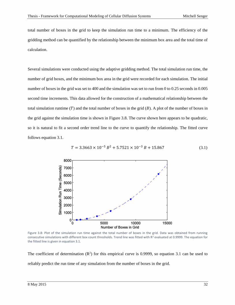
total number of boxes in the grid to keep the simulation run time to a minimum. The efficiency of the
gridding method can be quantified by the relationship between the minimum box area and the total time of
calculation.
Several simulations were conducted using the adaptive gridding method. The total simulation run time, the
number of grid boxes, and the minimum box area in the grid were recorded for each simulation. The initial
number of boxes in the grid was set to 400 and the simulation was set to run from 0 to 0.25 seconds in 0.005
second time increments. This data allowed for the construction of a mathematical relationship between the
total simulation runtime (𝑇) and the total number of boxes in the grid (𝐵). A plot of the number of boxes in
the grid against the simulation time is shown in Figure 3.8. The curve shown here appears to be quadratic,
so it is natural to fit a second order trend line to the curve to quantify the relationship. The fitted curve
follows equation 3.1.
𝑇 = 3.3663 × 10⁻⁵ 𝐵2 + 5.7521 × 10⁻³ 𝐵 + 15.867 (3.1)
The coefficient of determination (R2) for this empirical curve is 0.9999, so equation 3.1 can be used to
reliably predict the run time of any simulation from the number of boxes in the grid.
Figure 3.8: Plot of the simulation run time against the total number of boxes in the grid. Data was obtained from running consecutive simulations with different box count thresholds. Trend line was fitted with R2 evaluated at 0.9999. The equation for the fitted line is given in equation 3.1.
Thesis - Framework for Computational Modeling of Cellular Diffusion Systems Mitchell Senger
8 May 2015 33
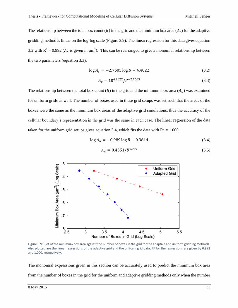
The relationship between the total box count (𝐵) in the grid and the minimum box area (𝐴𝑟) for the adaptive
gridding method is linear on the log-log scale (Figure 3.9). The linear regression for this data gives equation
3.2 with R2 = 0.992 (𝐴𝑟 is given in µm2). This can be rearranged to give a monomial relationship between
the two parameters (equation 3.3).
log 𝐴𝑟 = −2.7605 log 𝐵 + 4.4022 (3.2)
𝐴𝑟 = 104.4022/𝐵−2.7605 (3.3)
The relationship between the total box count (𝐵) in the grid and the minimum box area (𝐴𝑢) was examined
for uniform grids as well. The number of boxes used in these grid setups was set such that the areas of the
boxes were the same as the minimum box areas of the adaptive grid simulations, thus the accuracy of the
cellular boundary’s representation in the grid was the same in each case. The linear regression of the data
taken for the uniform grid setups gives equation 3.4, which fits the data with R2 = 1.000.
log 𝐴𝑢 = −0.989 log 𝐵 − 0.3614 (3.4)
𝐴𝑢 = 0.4351/𝐵0.989 (3.5)
The monomial expressions given in this section can be accurately used to predict the minimum box area
from the number of boxes in the grid for the uniform and adaptive gridding methods only when the number
Figure 3.9: Plot of the minimum box area against the number of boxes in the grid for the adaptive and uniform gridding methods. Also plotted are the linear regressions of the adaptive grid and the uniform grid data; R2 for the regressions are given by 0.992 and 1.000, respectively.
Thesis - Framework for Computational Modeling of Cellular Diffusion Systems Mitchell Senger
8 May 2015 34
of boxes is greater than roughly 400. The expressions will diverge from measured values when tested
against the areas of boxes in grids with a small total number of boxes.
Thesis - Framework for Computational Modeling of Cellular Diffusion Systems Mitchell Senger
8 May 2015 35
Chapter 4 – Discussion
4.1 Time Step Size Solution
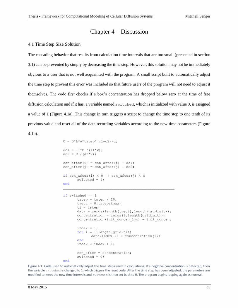
The cascading behavior that results from calculation time intervals that are too small (presented in section
3.1) can be prevented by simply by decreasing the time step. However, this solution may not be immediately
obvious to a user that is not well acquainted with the program. A small script built to automatically adjust
the time step to prevent this error was included so that future users of the program will not need to adjust it
themselves. The code first checks if a box’s concentration has dropped below zero at the time of free
diffusion calculation and if it has, a variable named switched, which is initialized with value 0, is assigned
a value of 1 (Figure 4.1a). This change in turn triggers a script to change the time step to one tenth of its
previous value and reset all of the data recording variables according to the new time parameters (Figure
4.1b).
C = D*L*w*tstep*(c1-c2)/d;
dc1 = -1*C /(A1*w); dc2 = C /(A2*w);
con_after(i) = con_after(i) + dc1; con_after(j) = con_after(j) + dc2;
if con_after(i) < 0 || con_after(j) < 0
switched = 1; end _____________________________________________________
if switched == 1 tstep = tstep / 10; tvect = 0:tstep:tmax; ti = tstep; data = zeros(length(tvect),length(gridinit)); concentration = zeros(1,length(gridinit)); concentration(init_concen_loc) = init_concen;
index = 1; for i = 1:length(gridinit)
data(index,i) = concentration(i); end index = index + 1;
con_after = concentration; switched = 0;
end
Figure 4.1: Code used to automatically adjust the time steps used in calculations. If a negative concentration is detected, then the variable switched is changed to 1, which triggers the reset code. After the time step has been adjusted, the parameters are modified to meet the new time intervals and switched is then set back to 0. The program begins looping again as normal.
Thesis - Framework for Computational Modeling of Cellular Diffusion Systems Mitchell Senger
8 May 2015 36
Once the reset is complete, switched is reassigned 0, and the calculations start over using the new time
step. This process can be repeated an arbitrary number of times until the time intervals are short enough to
accurately represent the system. This code should prevent the cascading effects from occurring during
simulation no matter which preset values are used.
The number of calculations performed in the course of the simulation in proportional to the inverse of the
time interval used in calculations. If the time interval is decreased by a factor of ten, then the number of
calculations that need to be carried out in the simulation increases by a factor of 10. The increase in
predicted simulation runtime due to the decrease in time intervals is reported to the user by a printed
statement.
4.2 Diffusion Simulations
While the constructed simulation does not model real cellular responses, it does give some insight to the
movement of particles due to free diffusion. The movement of particles in a region is regulated by the
diffusion coefficient in the region. The larger the coefficient, the faster the particles enter and leave a box
in the grid. This behavior is immediately apparent in the plots of Figure 3.2. Figure 3.2b shows the
concentration of particles over time in the box where the initial deposit was located for simulations using
different diffusion coefficients. As the coefficient increases, the rate that the particle concentration in the
box depletes also increases.
The concentration of particles in boxes near the box with the initial deposit exhibit slightly different
behavior. Particles leave the box faster with higher diffusion coefficients, but they also enter the box more
quickly. The concentration in a box near the initial deposit will maximize faster and will fall off more
quickly as the diffusion coefficient increases (Figure 3.2c, 3.2d). The maximal concentration in these boxes
does not change noticeably with changes in the diffusion coefficient of the system. While the rate of
Thesis - Framework for Computational Modeling of Cellular Diffusion Systems Mitchell Senger
8 May 2015 37
particles moving through the box near the initial deposit increases, the amount of particles moving through
it will be the same for any diffusion coefficient, and the rate at which particles enter and leave compensate
each other in such a way that the highest concentration the box will achieve will not change with the particle
movement rate.
In a system where the diffusion coefficient is larger in a compartment than the intracellular area, the
particles will spread from the initial deposit box if the initial deposit is located in a compartment than if it
had been outside the compartment but still inside the cell (Figure 3.3). However, because the particles
spread the maximum concentration in the cell will never be as large a system where the initial deposit is in
the intracellular area (Figure 3.3).
The mechanics of free diffusion are of paramount importance to simulations of intracellular ion action
because any free particles in the cell will experience it. The inclusion of these mechanics makes the
framework suitable to act as the backbone of more specific and complicated simulation programs in the
future.
4.3 Logistic Growth Mechanism
The inclusion of the logistic growth framework in the simulation program provides it with the means to
model simplified cellular reactions. Logistic growth drives the concentration of a region to an equilibrium
value, and is calculated in simulations using equation 1.10. The scaling factor (𝛼 in equation 1.10) is the
mathematical representation of the magnitude to which the cell responds to the presence of particles. A
large scaling factor corresponds to a cell or compartment that quickly drives the concentration to
equilibrium, and a small factor corresponds to a cell with a softer response (Figure 3.5). The way the model
adds or removes particles to achieve equilibrium is essentially a simplified cellular reaction. Compartment
responses can be modeled by limiting the logistic growth behavior to the compartments of the cell (Figure
3.6, 3.7)
Thesis - Framework for Computational Modeling of Cellular Diffusion Systems Mitchell Senger
8 May 2015 38
The code used to calculate cellular reactions to particles can be manipulated so that the behavior only occurs
in certain regions within the cell. The entire cellular space can be modeled to exhibit logistic growth, or it
can be limited to a single compartment. The flexibility of this programming will allow the framework to be
adapted to model many different cellular reaction processes.
4.4 Adaptive Grid Performance
Smaller grid boxes at the boundary of cellular compartments increases the accuracy of the boundary’s
representation in the grid. However, the use of smaller boxes increases the total number of boxes, which in
turn increases the simulation run time. The accuracy of the model does not increase from the use of smaller
boxes. If the size of the boxes throughout the cell is uniform, then the boxes in regions where there are no
boundaries are smaller than the model needs them to be. Therefore the use of a uniform grid wastes
simulation time.
The adaptive grid used in this model increases the number of boxes and decreases their area when they are
on or near a boundary, but leaves boxes far from the boundary at their original size. Using an adaptive grid
rather than a uniform grid greatly reduces the total number of boxes in the grid while simultaneously
minimizing the box area at the boundary, thus reducing the simulation run time while maintaining the same
level of boundary representation accuracy.
The monomial expressions equations 3.3 and 3.5 show that the minimum box area of an adaptive grid scales
closely to 𝐵−3, while the minimum box area of the uniform grid scales like 𝐵−1. This means that accurately
representing a grid boundary can be achieved using much fewer boxes if an adaptive grid is used over the
uniform grid. For example, a simulation using an adaptive grid with a minimum box area of 1.75E-5 µm2
will run approximately 141 times faster than a simulation using a uniform grid. The adaptive gridding
method was needed to maintain simulation accuracy while still making usable in a laboratory setting.
Thesis - Framework for Computational Modeling of Cellular Diffusion Systems Mitchell Senger
8 May 2015 39
Chapter 5 – Conclusions
5.1 Current Framework
The current framework is able to spatially parameterize a single cell from a monochromatic image and
artificially generate compartments within the cell boundary. It can then overlay a grid with uniform box
thickness across the space of the cell and recursively adapt the size of the boxes in the grid to accurately
represent the boundary within the grid. Diffusion coefficients that are unique to the compartment that the
boxes lie in can be assigned to the planes between boxes. From these steps, the framework can simulate the
free diffusion of a deposit of particles through the cell over time. Because the simulation programs will be
adapted to account for realistic cellular reaction mechanisms, logistic growth calculations, which act as a
simplified reaction mechanism, were included in the code to act as a place holder for more realistic cellular
reaction processes.
5.2 Simulation Usability
This framework will act as the backbone for simulations of real cellular diffusion processes that will be
used in experimental labs in the future. Because of this, the simulation is equipped with code that prints the
progress of the calculations as they are performed in the form of a percentage of calculations complete or
an estimated time remaining. It also distinguishes between when the program is initializing the grid and
when the diffusion calculations are taking place. These features are included to inform the user of the
progress of the simulation as it is actively running.
The program that conducts diffusion and reaction calculations (Appendix D) outputs the concentration of
every box in every time step specified by the user, but the numerical outputs by themselves are not telling
of the particle behavior during the simulation. Because of this, several short scripts have been developed to
display the concentrations of the boxes over time. One script, called plot_boxes, accepts the indices of
Thesis - Framework for Computational Modeling of Cellular Diffusion Systems Mitchell Senger
8 May 2015 40
any boxes of interest as an input and plots the concentration over time for each box (Appendix E). This
function was used to generate the plots displayed in Figures 3.1, 3.2, 3.5, and 3.6. This is a fast and
convenient way to see localized particle behavior over the course of a simulation. Another script called
color_plot, plots the concentration of every box in a contour plot using color coordination to display the
concentration in the entire region of the cell. The plot is then animated for each time step, and the plots are
saved to an AVI file (Appendix F). The change of concentration throughout the whole cell over time can
then be viewed as a short movie. Frames from these animations were used to generate Figures 3.3, 3.4, and
3.7.
5.3 Future Development of Simulations
This code will be used as the framework for simulations that model Ca2+ action in a multicellular system.
For this to work, several more features need to be included. The cellular boundary is parameterized in two
dimensions and then given a uniform thickness that is small compared to the height and width of the cell.
For the simulation to model real systems, the cells need to be parameterized in three dimensions. To do
this, multiple layers of a cell will need to be imaged and parameterized using im2poly, and the initialization
code, grid_overlay2, will need to interpolate the layers into a three dimensional boundary.
Ca2+ concentration in a cell is regulated by channels on the surface of the endoplasmic reticulum that open
or close due to the presence of intracellular IP3 [6]. IP3 moves through the cell by free diffusion like the
Ca2+ ions, so to model this action, the simulation will need to track the concentration of two separate species
simultaneously. Channel action can be modeled in the existing code by manipulating the diffusion
coefficients of planes between boxes of different compartments. Also, cells are not isolated systems; Ca2+
behavior in one cell is influenced by the concentration of Ca2+ in other cells nearby. Another goal for the
cellular model is to simulate the diffusion of ions in a multicellular array. To do this, multiple cells will be
parameterized, and the initialization code will be adapted to “stitch” the grids overlaying single cells into
Thesis - Framework for Computational Modeling of Cellular Diffusion Systems Mitchell Senger
8 May 2015 41
one large grid that can simulate particle flow. The inclusion of multicellular system compatibility, three
dimensional parameterization, and the ability to track the concentration of multiple species at once will
make the framework ready for lab use.
Thesis - Framework for Computational Modeling of Cellular Diffusion Systems Mitchell Senger
8 May 2015 42
References
[1] Cao, P., Donovan, G., Falcke, M., & Sneyd, J. (2013). A Stochastic Model of Calcium Puffs
Based on Single-Channel Data. Biophysical Journal, 105, 1133-1142.
[2] Doi, M., & Edwards, S. (1986). Brownian Motion. In The theory of polymer dynamics (pp. 46-
47). Clarendon Press.
[3] Image Processing Toolbox. (n.d.). Retrieved June 1, 2014, from
http://www.mathworks.com/help/images/examples/detecting-a-cell-using-image-
segmentation.html?prodcode=IP
[4] Meyer, P., Yung, J., & Ausubel, J. (1999). A Primer on Logistic Growth and Substitution: The
Mathematics of the Loglet Lab Software. Technological Forecasting and Social Change, 61(3),
247-271.
[5] Petker, J. (2010, April 1). Point-in-Polygon Detection. Retrieved December 5, 2014.
[6] Tang, Y., & Othmer, H. (1995). Frequency Encoding in Excitable Systems with Applications to
Calcium Oscillations. Proceedings of the National Academy of Sciences, 92, 7869-7873.
Thesis - Framework for Computational Modeling of Cellular Diffusion Systems Mitchell Senger
8 May 2015 43
Appendices
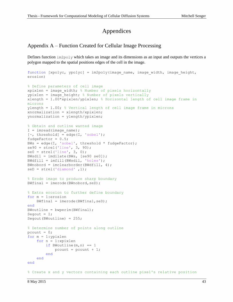
Appendix A – Function Created for Cellular Image Processing
Defines function im2poly which takes an image and its dimensions as an input and outputs the vertices a
polygon mapped to the spatial positions edges of the cell in the image.
function [xpolyc, ypolyc] = im2poly(image_name, image_width, image_height,
erosion)
% Define parameters of cell image xpixlen = image_width; % Number of pixels horizontally ypixlen = image_height; % Number of pixels vertically xlength = 1.00*xpixlen/ypixlen; % Horizontal length of cell image frame in
microns ylength = 1.00; % Vertical length of cell image frame in microns xnormalization = xlength/xpixlen; ynormalization = ylength/ypixlen;
% Obtain and outline wanted image I = imread(image_name); [~, threshold] = edge(I, 'sobel'); fudgeFactor = 0.5; BWs = edge(I, 'sobel', threshold * fudgeFactor); se90 = strel('line', 3, 90); se0 = strel('line', 3, 0); BWsdil = imdilate(BWs, [se90 se0]); BWdfill = imfill(BWsdil, 'holes'); BWnobord = imclearborder(BWdfill, 4); seD = strel('diamond' ,1);
% Erode image to produce sharp boundary BWfinal = imerode(BWnobord,seD);
% Extra erosion to further define boundary for m = 1:erosion BWfinal = imerode(BWfinal,seD); end BWoutline = bwperim(BWfinal); Segout = I; Segout(BWoutline) = 255;
% Determine number of points along outline pcount = 0; for m = 1:ypixlen for n = 1:xpixlen if BWoutline(m,n) == 1 pcount = pcount + 1; end end end
% Create x and y vectors containing each outline pixel's relative position
Thesis - Framework for Computational Modeling of Cellular Diffusion Systems Mitchell Senger
8 May 2015 44
xvect = zeros([pcount,1]); yvect = zeros([pcount,1]);
xin = 1; yin = 1; zin = 1;
for m = 1:ypixlen for n = 1:xpixlen if BWoutline(m,n) == 1 xvect(xin,1) = n*xnormalization; yvect(yin,1) = m*ynormalization; xin = xin + 1; yin = yin + 1; end end end clear xin yin
xinit = xvect(1,1); yinit = yvect(1,1);
xori = xvect; yori = yvect;
x0 = xinit; y0 = yinit; d0 = 100000;
xpoly = zeros([pcount,1]); ypoly = zeros([pcount,1]);
mini = 1;
% Reorder points in xvect and yvect to create polygon
% Define error to width ratio etwr = 61;
for j = 1:pcount d0 = 100000; x0 = xvect(mini,1); y0 = yvect(mini,1); xvect(mini,1) = 0; yvect(mini,1) = 0; for i = 1:pcount x = xvect(i,1); y = yvect(i,1); d = (x-x0)^2 + (y-y0)^2; if d < d0 d0 = d; mini = i; end end xpoly(j,1) = x0;
Thesis - Framework for Computational Modeling of Cellular Diffusion Systems Mitchell Senger
8 May 2015 45
ypoly(j,1) = y0; if d0 > xlength/etwr break end end
% Close the polygon and remove any leftover zeros xpoly = xpoly(xpoly~=0); ypoly = ypoly(ypoly~=0); xpoly(length(xpoly)+1,1) = xinit; ypoly(length(ypoly)+1,1) = yinit; ypoly = -1*ypoly;
% Center cell polygon xavg = (max(xpoly) + min(xpoly))/2; yavg = (max(ypoly) + min(ypoly))/2;
xpolyc = xpoly - xavg; ypolyc = ypoly - yavg;
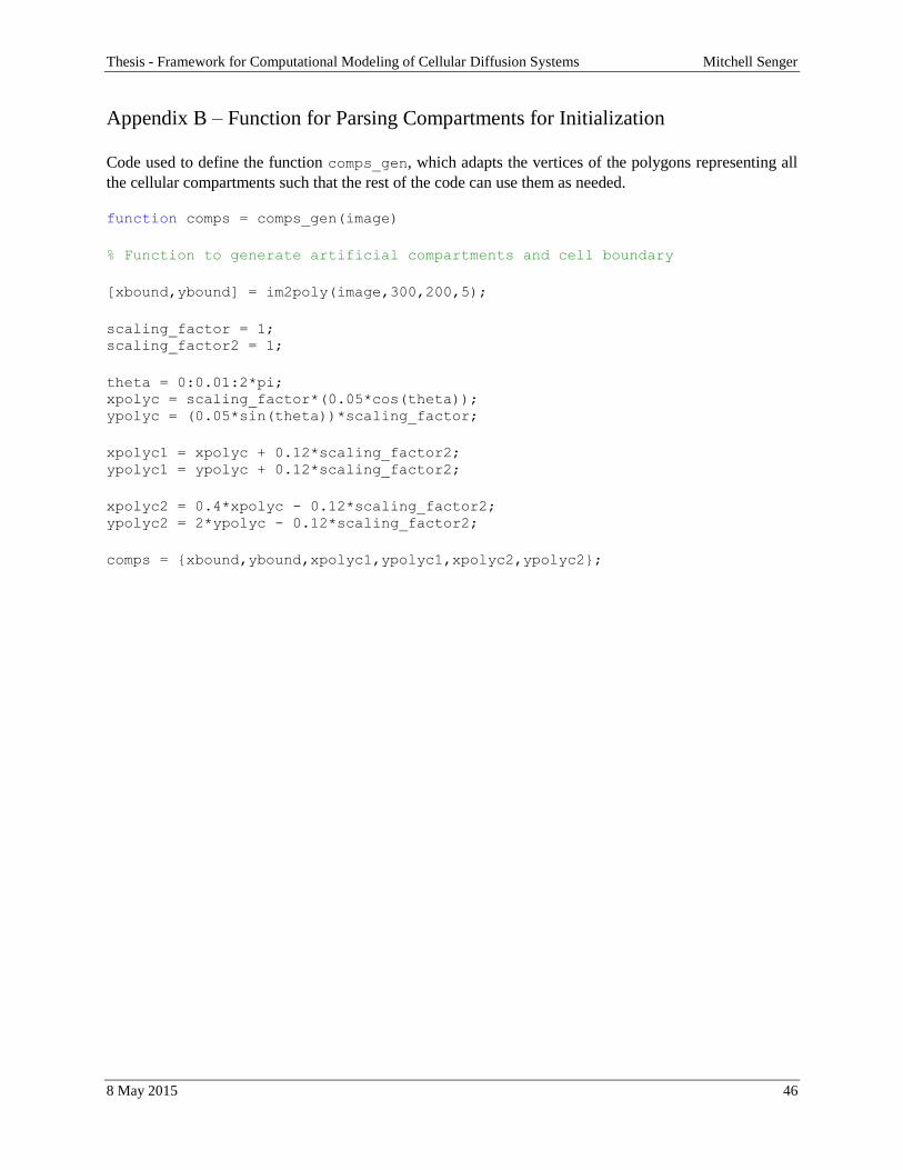
Thesis - Framework for Computational Modeling of Cellular Diffusion Systems Mitchell Senger
8 May 2015 46
Appendix B – Function for Parsing Compartments for Initialization
Code used to define the function comps_gen, which adapts the vertices of the polygons representing all
the cellular compartments such that the rest of the code can use them as needed.
function comps = comps_gen(image)
% Function to generate artificial compartments and cell boundary
[xbound,ybound] = im2poly(image,300,200,5);
scaling_factor = 1; scaling_factor2 = 1;
theta = 0:0.01:2*pi; xpolyc = scaling_factor*(0.05*cos(theta)); ypolyc = (0.05*sin(theta))*scaling_factor;
xpolyc1 = xpolyc + 0.12*scaling_factor2; ypolyc1 = ypolyc + 0.12*scaling_factor2;
xpolyc2 = 0.4*xpolyc - 0.12*scaling_factor2; ypolyc2 = 2*ypolyc - 0.12*scaling_factor2;
comps = {xbound,ybound,xpolyc1,ypolyc1,xpolyc2,ypolyc2};
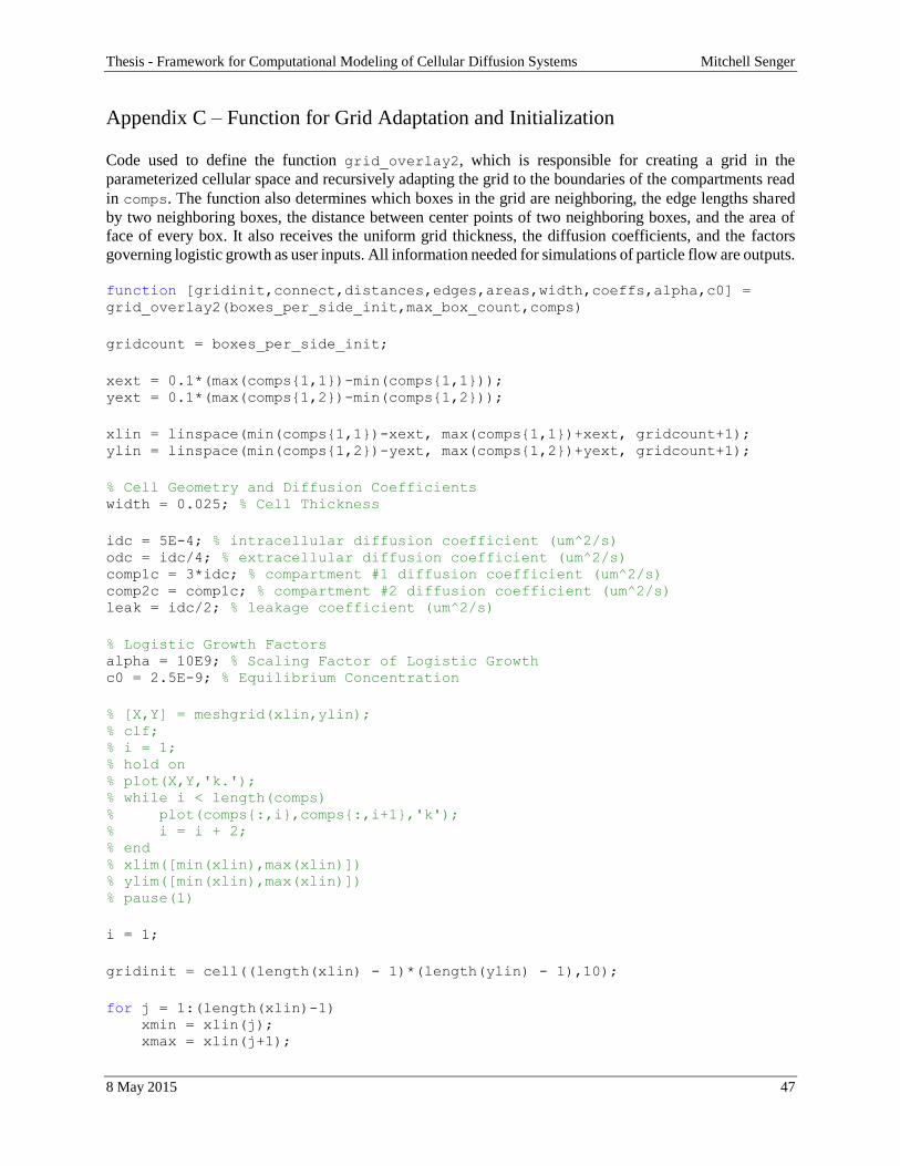
Thesis - Framework for Computational Modeling of Cellular Diffusion Systems Mitchell Senger
8 May 2015 47
Appendix C – Function for Grid Adaptation and Initialization
Code used to define the function grid_overlay2, which is responsible for creating a grid in the
parameterized cellular space and recursively adapting the grid to the boundaries of the compartments read
in comps. The function also determines which boxes in the grid are neighboring, the edge lengths shared
by two neighboring boxes, the distance between center points of two neighboring boxes, and the area of
face of every box. It also receives the uniform grid thickness, the diffusion coefficients, and the factors
governing logistic growth as user inputs. All information needed for simulations of particle flow are outputs.
function [gridinit,connect,distances,edges,areas,width,coeffs,alpha,c0] =
grid_overlay2(boxes_per_side_init,max_box_count,comps)
gridcount = boxes_per_side_init;
xext = 0.1*(max(comps{1,1})-min(comps{1,1})); yext = 0.1*(max(comps{1,2})-min(comps{1,2}));
xlin = linspace(min(comps{1,1})-xext, max(comps{1,1})+xext, gridcount+1); ylin = linspace(min(comps{1,2})-yext, max(comps{1,2})+yext, gridcount+1);
% Cell Geometry and Diffusion Coefficients width = 0.025; % Cell Thickness
idc = 5E-4; % intracellular diffusion coefficient (um^2/s) odc = idc/4; % extracellular diffusion coefficient (um^2/s) comp1c = 3*idc; % compartment #1 diffusion coefficient (um^2/s) comp2c = comp1c; % compartment #2 diffusion coefficient (um^2/s) leak = idc/2; % leakage coefficient (um^2/s)
% Logistic Growth Factors alpha = 10E9; % Scaling Factor of Logistic Growth c0 = 2.5E-9; % Equilibrium Concentration
% [X,Y] = meshgrid(xlin,ylin); % clf; % i = 1; % hold on % plot(X,Y,'k.'); % while i < length(comps) % plot(comps{:,i},comps{:,i+1},'k'); % i = i + 2; % end % xlim([min(xlin),max(xlin)]) % ylim([min(xlin),max(xlin)]) % pause(1)
i = 1;
gridinit = cell((length(xlin) - 1)*(length(ylin) - 1),10);
for j = 1:(length(xlin)-1) xmin = xlin(j); xmax = xlin(j+1);
Thesis - Framework for Computational Modeling of Cellular Diffusion Systems Mitchell Senger
8 May 2015 48
for k = 1:(length(ylin)-1) ymin = ylin(k+1); ymax = ylin(k);
xs = [xmax; xmax; xmin; xmin; xmax]; ys = [ymax; ymin; ymin; ymax; ymax];
gridinit{i,1} = xs; gridinit{i,2} = ys; i = i + 1; end end
n = 0; p = 1;
while length(gridinit) <= max_box_count for i = 1:length(gridinit) xs = gridinit{i,1}; ys = gridinit{i,2}; warning('off','map:polygon:noExternalContours');
j = 1; k = 1;
while j < length(comps) xpoly = comps{1,j}; ypoly = comps{1,j+1}; in = inpolygon(xpoly,ypoly,xs,ys); [xin,yin] = polybool('intersection', xs, ys, xpoly, ypoly); xin(find(isnan(xin),1)) = []; yin(find(isnan(yin),1)) = [];
if sum(in) > 0 xmin = min(xs); ymin = min(ys); xmax = max(xs); ymax = max(ys); xnew = (xmax + xmin)/2; ynew = (ymax + ymin)/2;
xco = [xmin,xnew,xmax]; yco = [ymin,ynew,ymax];
x1 = [xco(1);xco(1);xco(2);xco(2);xco(1)]; y1 = [yco(1);yco(2);yco(2);yco(1);yco(1)];
Thesis - Framework for Computational Modeling of Cellular Diffusion Systems Mitchell Senger
8 May 2015 49
x2 = [xco(1);xco(1);xco(2);xco(2);xco(1)]; y2 = [yco(2);yco(3);yco(3);yco(2);yco(2)];
x3 = [xco(2);xco(2);xco(3);xco(3);xco(2)]; y3 = [yco(2);yco(3);yco(3);yco(2);yco(2)];
x4 = [xco(2);xco(2);xco(3);xco(3);xco(2)]; y4 = [yco(1);yco(2);yco(2);yco(1);yco(1)];
gridinit{i,1} = x1; gridinit{i,2} = y1;
L = length(gridinit);
gridinit{L+1,1} = x2; gridinit{L+1,2} = y2;
gridinit{L+2,1} = x3; gridinit{L+2,2} = y3;
gridinit{L+3,1} = x4; gridinit{L+3,2} = y4;
end j = j + 2; k = k + 1; end end end
for i = 1:length(gridinit) initialization_percent_complete = 100*i/(length(gridinit)) xmax = max(gridinit{i,1}); xmin = min(gridinit{i,1}); ymax = max(gridinit{i,2}); ymin = min(gridinit{i,2});
for j = 1:length(gridinit) if j ~= i xmax_t = max(gridinit{j,1}); xmin_t = min(gridinit{j,1}); ymax_t = max(gridinit{j,2}); ymin_t = min(gridinit{j,2});
if ymin_t == ymax || ymin == ymax_t if (xmin_t >= xmin && xmax >= xmax_t) || (xmin_t <= xmin &&
xmax <= xmax_t) gridinit{i,4}(length(gridinit{i,4}) + 1) = j; end end
if xmin_t == xmax || xmin == xmax_t
Thesis - Framework for Computational Modeling of Cellular Diffusion Systems Mitchell Senger
8 May 2015 50
if (ymin_t >= ymin && ymax >= ymax_t) || (ymin_t <= ymin &&
ymax <= ymax_t) gridinit{i,4}(length(gridinit{i,4}) + 1) = j; end end end end end
connect = zeros(length(gridinit),length(gridinit));
for i = 1:length(gridinit) for j = gridinit{i,4} connect(j,i) = 1; end end
distances = zeros(length(gridinit),length(gridinit)); edges = zeros(length(gridinit),length(gridinit));
for i = 1:length(gridinit) for j = 1:length(gridinit) if connect(i,j) == 1 xmaxi = max(gridinit{i,1}); xmini = min(gridinit{i,1});
ymaxi = max(gridinit{i,2}); ymini = min(gridinit{i,2});
xmaxj = max(gridinit{j,1}); xminj = min(gridinit{j,1});
ymaxj = max(gridinit{j,2}); yminj = min(gridinit{j,2});
xi = (xmaxi + xmini)/2; yi = (ymaxi + ymini)/2; xj = (xmaxj + xminj)/2; yj = (ymaxj + yminj)/2;
distances(i,j) = sqrt((xi-xj)^2 + (yi-yj)^2);
if ymaxj == ymini || yminj == ymaxi pos = [(xmaxj-xminj),(xmaxi-xmini)]; end
if xmaxj == xmini || xminj == xmaxi pos = [(ymaxj-yminj),(ymaxi-ymini)]; end
edges(i,j) = min(pos); end end end
Thesis - Framework for Computational Modeling of Cellular Diffusion Systems Mitchell Senger
8 May 2015 51
warning off for i = 1:length(gridinit) xs = gridinit{i,1}; ys = gridinit{i,2}; gridinit{i,3} = zeros(1,(length(comps)/2) + 1);
j = 1; k = 2; while j < length(comps) xpoly = comps{1,j}; ypoly = comps{1,j+1}; in = inpolygon(xs,ys,xpoly,ypoly);
if sum(in) == 5 gridinit{i,3}(k) = 1; end
if sum(in) == 0 gridinit{i,3}(k) = 0; end
if sum(in) ~= 0 && sum(in) ~= 5 [xin,yin] = polybool('intersection', xs, ys, xpoly, ypoly); xin(find(isnan(xin),1)) = []; yin(find(isnan(yin),1)) = [];
total_area = polyarea(xs,ys); inside_area = polyarea(xin,yin);
if inside_area >= total_area/2 gridinit{i,3}(k) = 1; end
if inside_area < total_area/2 gridinit{i,3}(k) = 0; end end j = j + 2; k = k + 1; end
if gridinit{i,3} == zeros(1,(length(comps)/2) + 1); gridinit{i,3}(1) = 1; end for k = 3:length(gridinit{i,3}); if gridinit{i,3}(k) == 1 gridinit{i,3}(2) = 0; end end end warning on
areas = zeros(1,length(gridinit)); for i = 1:length(gridinit)
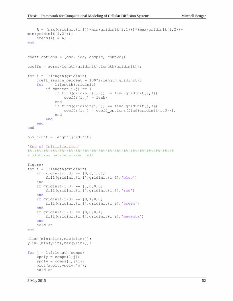
Thesis - Framework for Computational Modeling of Cellular Diffusion Systems Mitchell Senger
8 May 2015 52
A = (max(gridinit{i,1})-min(gridinit{i,1}))*(max(gridinit{i,2})-
min(gridinit{i,2})); areas(i) = A; end
coeff_options = [odc, idc, comp1c, comp2c];
coeffs = zeros(length(gridinit),length(gridinit));
for i = 1:length(gridinit) coeff_assign_percent = 100*i/length(gridinit); for j = 1:length(gridinit) if connect(i,j) == 1 if find(gridinit{i,3}) ~= find(gridinit{j,3}) coeffs(i,j) = leak; end if find(gridinit{i,3}) == find(gridinit{j,3}) coeffs(i,j) = coeff_options(find(gridinit{i,3})); end end end end
box_count = length(gridinit)
'End of Initialization' %%%%%%%%%%%%%%%%%%%%%%%%%%%%%%%%%%%%%%%%%%%%%%%%%%%%%%%%%%%%%%%% % Plotting parameterized cell
figure; for i = 1:length(gridinit) if gridinit{i,3} == [0,0,1,0]; fill(gridinit{i,1},gridinit{i,2},'blue') end if gridinit{i,3} == [1,0,0,0] fill(gridinit{i,1},gridinit{i,2},'red') end if gridinit{i,3} == [0,1,0,0] fill(gridinit{i,1},gridinit{i,2},'green') end if gridinit{i,3} == [0,0,0,1] fill(gridinit{i,1},gridinit{i,2},'magenta') end hold on end
xlim([min(xlin),max(xlin)]); ylim([min(ylin),max(ylin)]);
for j = 1:2:length(comps) xpoly = comps{1,j}; ypoly = comps{1,j+1}; plot(xpoly,ypoly,'w'); hold on
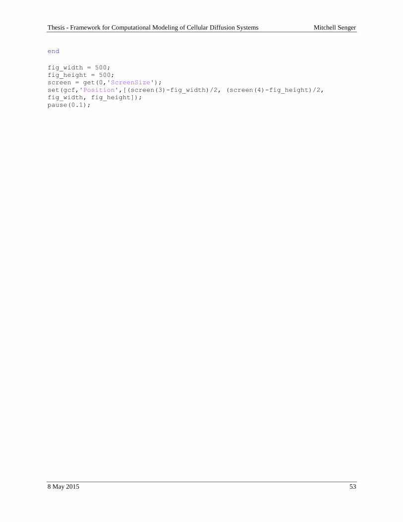
Thesis - Framework for Computational Modeling of Cellular Diffusion Systems Mitchell Senger
8 May 2015 53
end
fig_width = 500; fig_height = 500; screen = get(0,'ScreenSize'); set(gcf,'Position',[(screen(3)-fig_width)/2, (screen(4)-fig_height)/2,
fig_width, fig_height]); pause(0.1);
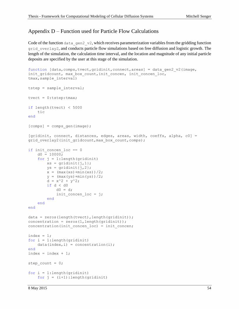
Thesis - Framework for Computational Modeling of Cellular Diffusion Systems Mitchell Senger
8 May 2015 54
Appendix D – Function used for Particle Flow Calculations
Code of the function data_gen2_v2, which receives parameterization variables from the gridding function
grid_overlay2, and conducts particle flow simulations based on free diffusion and logistic growth. The
length of the simulation, the calculation time interval, and the location and magnitude of any initial particle
deposits are specified by the user at this stage of the simulation.
function [data,comps,tvect,gridinit,connect,areas] = data_gen2_v2(image,
init_gridcount, max_box_count,init_concen, init_concen_loc,
tmax,sample_interval)
tstep = sample_interval;
tvect = 0:tstep:tmax;
if length(tvect) < 5000 tic end
[comps] = comps_gen(image);
[gridinit, connect, distances, edges, areas, width, coeffs, alpha, c0] =
grid_overlay2(init_gridcount,max_box_count,comps);
if init_concen_loc == 0 d0 = 10000; for j = 1:length(gridinit) xs = gridinit{j,1}; ys = gridinit{j,2}; x = (max(xs)+min(xs))/2; y = (max(ys)+min(ys))/2; d = x^2 + y^2; if d < d0 d0 = d; init_concen_loc = j; end end end
data = zeros(length(tvect),length(gridinit)); concentration = zeros(1,length(gridinit)); concentration(init_concen_loc) = init_concen;
index = 1; for i = 1:length(gridinit) data(index,i) = concentration(i); end index = index + 1;
step_count = 0;
for i = 1:length(gridinit) for j = (i+1):length(gridinit)
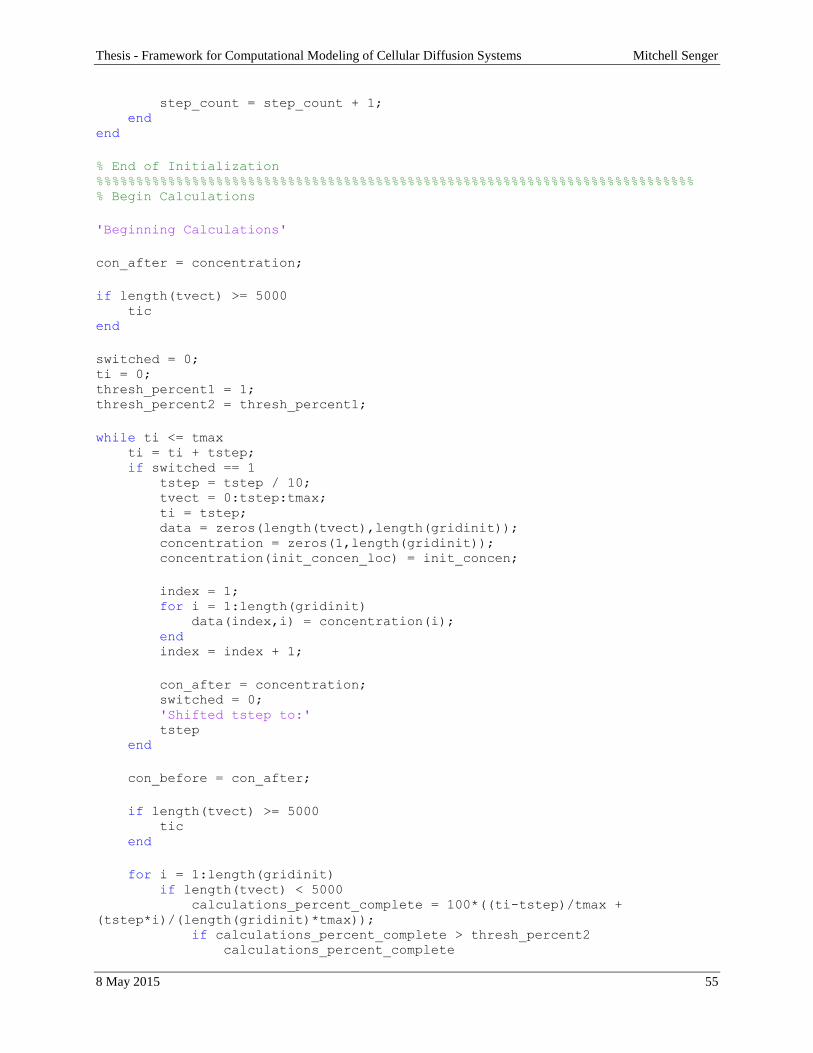
Thesis - Framework for Computational Modeling of Cellular Diffusion Systems Mitchell Senger
8 May 2015 55
step_count = step_count + 1; end end
% End of Initialization %%%%%%%%%%%%%%%%%%%%%%%%%%%%%%%%%%%%%%%%%%%%%%%%%%%%%%%%%%%%%%%%%%%%%%%%%%% % Begin Calculations
'Beginning Calculations'
con_after = concentration;
if length(tvect) >= 5000 tic end
switched = 0; ti = 0; thresh_percent1 = 1; thresh_percent2 = thresh_percent1;
while ti <= tmax ti = ti + tstep; if switched == 1 tstep = tstep / 10; tvect = 0:tstep:tmax; ti = tstep; data = zeros(length(tvect),length(gridinit)); concentration = zeros(1,length(gridinit)); concentration(init_concen_loc) = init_concen;
index = 1; for i = 1:length(gridinit) data(index,i) = concentration(i); end index = index + 1;
con_after = concentration; switched = 0; 'Shifted tstep to:' tstep end
con_before = con_after;
if length(tvect) >= 5000 tic end
for i = 1:length(gridinit) if length(tvect) < 5000 calculations_percent_complete = 100*((ti-tstep)/tmax +
(tstep*i)/(length(gridinit)*tmax)); if calculations_percent_complete > thresh_percent2 calculations_percent_complete
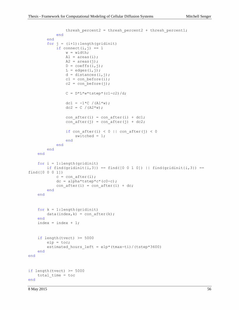
Thesis - Framework for Computational Modeling of Cellular Diffusion Systems Mitchell Senger
8 May 2015 56
thresh_percent2 = thresh_percent2 + thresh_percent1; end end for j = (i+1):length(gridinit) if connect(i,j) == 1 w = width; A1 = areas(i); A2 = areas(j); D = coeffs(i,j); L = edges(i,j); d = distances(i,j); c1 = con_before(i); c2 = con_before(j);
C = D*L*w*tstep*(c1-c2)/d;
dc1 = -1*C /(A1*w); dc2 = C /(A2*w);
con_after(i) = con_after(i) + dc1; con_after(j) = con_after(j) + dc2;
if con_after(i) < 0 || con_after(j) < 0 switched = 1; end end end end
for i = 1:length(gridinit) if find(gridinit{i,3}) == find([0 0 1 0]) || find(gridinit{i,3}) ==
find([0 0 0 1]) c = con_after(i); dc = alpha*tstep*c*(c0-c); con_after(i) = con_after(i) + dc; end end
for k = 1:length(gridinit) data(index,k) = con_after(k); end index = index + 1;
if length(tvect) >= 5000 elp = toc; estimated_hours_left = elp*(tmax-ti)/(tstep*3600) end end
if length(tvect) >= 5000 total_time = toc end
Thesis - Framework for Computational Modeling of Cellular Diffusion Systems Mitchell Senger
8 May 2015 57
Appendix E – Function used for Displaying Box Concentration
Code used to plot the concentration of particles in grid boxes specified by the user from data generated by
the simulation.
function plot_boxes(tvect,data,boxes) figure; con = zeros(1,length(tvect)); colors = ['b','r','g','k','m','o','y']; index = 1;
legd_titles = {};
maxbef = 0;
for j = boxes for i = 1:length(tvect) con(1,i) = data(i,j); end maxcon = max(con);
if maxcon > maxbef maxbef = maxcon; end
plot(tvect,con,colors(index)); hold on
legd_titles{index} = sprintf('Box Index %d',j);
index = index + 1; end
ylim([0 1.1*maxbef]); ylabel('Concentration (nmol/\mum^{3})') xlabel('Time (Seconds)') legend(legd_titles); dims = get(gcf,'Position'); set(gcf,'Position',[dims(1), dims(2), 465, 283])
Thesis - Framework for Computational Modeling of Cellular Diffusion Systems Mitchell Senger
8 May 2015 58
Appendix F – Function used for Plotting and Animating Cell Concentrations
Code for the function color_plot, which uses the data generated from a simulation to plot the
concentration of each box for each time step in a color coordinated contour plot, then create a movie from
the animated plots.
function color_plot(tvect,data,gridinit,comps,frame_count,file_name)
xs = zeros(1,length(gridinit)); ys = zeros(1,length(gridinit));
for i = 1:length(gridinit) xavg = (max(gridinit{i,1})+min(gridinit{i,1}))/2; yavg = (max(gridinit{i,2})+min(gridinit{i,2}))/2; xs(i) = xavg; ys(i) = yavg; end
dx0 = 100; dy0 = 100;
xsu = unique(xs); ysu = unique(ys);
for i = 2:length(ysu) dy = abs(ysu(i) - ysu(i-1)); if dy < dy0 dy0 = dy; end end
for i = 2:length(xsu) dx = abs(xsu(i) - xsu(i-1)); if dx < dx0 dx0 = dx; end end
xgrid = transpose(min(xs):dx0:max(xs)); ygrid = transpose(min(ys):dy0:max(ys));
[X,Y] = meshgrid(xgrid,ygrid);
xs = transpose(xs); ys = transpose(ys);
tstep = tvect(2) - tvect(1); frametimes = linspace(0,max(tvect),frame_count); frametimes = tstep * floor(frametimes/tstep); frameindices = zeros(length(frametimes));
for i = 1:length(frametimes) if ~isempty(find(tvect == frametimes(i)))
Thesis - Framework for Computational Modeling of Cellular Diffusion Systems Mitchell Senger
8 May 2015 59
frameindices(i) = find(tvect == frametimes(i)); end end
mov = VideoWriter(file_name); mov.FrameRate = 15; mov.Quality = 100; open(mov);
fig = figure('Renderer','zbuffer'); axis tight manual; set(gcf,'PaperPositionMode','auto') set(fig,'DoubleBuffer','on'); set(gca,'NextPlot','replace','Visible','off');
for i = 1:length(frameindices) if frameindices(i) > 0 F = griddata(xs,ys,transpose(data(frameindices(i),:)),X,Y,'natural'); clf contourf(X,Y,F,'LineStyle','none') colorbar hold on for j = 1:2:length(comps) xpoly = comps{1,j}; ypoly = comps{1,j+1}; plot(xpoly,ypoly,'m'); hold on end str = sprintf('t = %g',frametimes(i)); title(str) dims = get(gcf,'Position'); set(gcf,'Position',[dims(1) dims(2) 375 300]); colormap(hot) frame = getframe(gcf); writeVideo(mov,frame); end end
close(fig); close(mov);
![Cellular automata approach to hybrid surface and diffusion ... · Cellular automata are therefore already commonly used for the modeling of chemical systems [1–11]. Cellular automata](https://img.pdfslide.us/doc/110x75/5f1ecf535b80731f8b25d3c6/cellular-automata-approach-to-hybrid-surface-and-diffusion-cellular-automata.jpg)