4321

Abstract

We propose a method for fusing a LIDAR point cloud to

camera data in real time, which will also backfill the myriad of data holes LIDAR creates. This is done in a way that also leverages the images features to weight how point clouds are filled. Multithreaded programing and GP-GPU methods allow us to obtain 10 fps with a Velodyne 64E LIDAR completely fused in 360º using a Ladybug panoramic camera. The method also generalizes to other kinds of point clouds such as those obtained by aerial vehicles. The primary advantage of our approach is it combines 360º fusion with upsampling in real time without mode smoothing.

1. Introduction This is a method which will take in a stream of frame

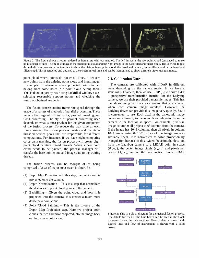
data from a 2D camera such as a standard video or panoramic camera, and it will fuse that data in real-time to a point cloud frame provided by a 3D metric sensor such as a LIDAR (see figure 1). The colored 3D point cloud, which is created by fusion, is denser than the original LIDAR point cloud. This is because we project pixels from the 2D video source back into the point cloud to fill in empty regions. Figure 2 shows an example.

Fusion is completed and rendered in real time. Here,

real time refers to the speed of the Velodyne 64E sensor that completes 10 360º sweeps per second. Thus, at 10 frames per second, image data is fetched from the 2D sensor and is painted onto the LIDAR data that natively has no color. This painted point cloud is then backfilled and the new colored backfilled point cloud is rendered and displayed for the user. The device also displays live output and can save streaming data at 10 fps. For practical purposes, we will refer to our demonstration system as a PanDAR (Panoramic EO / LIDAR).

Our approach can be contrasted with prior art in the

following ways. First, many prior works only deal with one or a few standard cameras fused to a 360º LIDAR scan and do not cover the full 360º with a camera [1]. Many methods use basic interpolation to try and fill back a point cloud [2]. Our method of backfilling attempts to be very careful in how it creates an interpolative effect. Some prior works do fusion of full 360º image to LIDAR but probably do not run at frame rate [3-5]. Also, many methods do not try to leverage camera data to help with filling but work primarily on local point cloud gradient data [6]. Compared with [7], this method puts emphasis on finding a small set of exemplar support points over which the most complex statistics are performed. This allows expensive point cloud gradients to be computed over the entire image area quickly without mode generalization that can aggressively smooth out surfaces. Each image pixel is essentially treated independently as it is back projected to the depth map. Ideally, this should help preserve texture.

2. The Fusion Process Overview The fusion process produces several outputs. The first

one is the painted point cloud. This is the image data projected out into the point cloud. The fusion process also returns a depth map which overlays the distance from camera to points in the image. This is interpretable as a type of image and the fusion process will create a color representation of the depth map and overlay the original image (see figures 1 and 4).

The fusion process is also responsible for backfilling the

point cloud. It does this by projecting image pixels into the

Frame Rate Fusion and Upsampling of EO/LIDAR Data for Multiple Platforms

T. Nathan Mundhenk, Kyungnam Kim, Yuri Owechko HRL Laboratories LLC

Malibu, California tnmundhenk@hrl.com

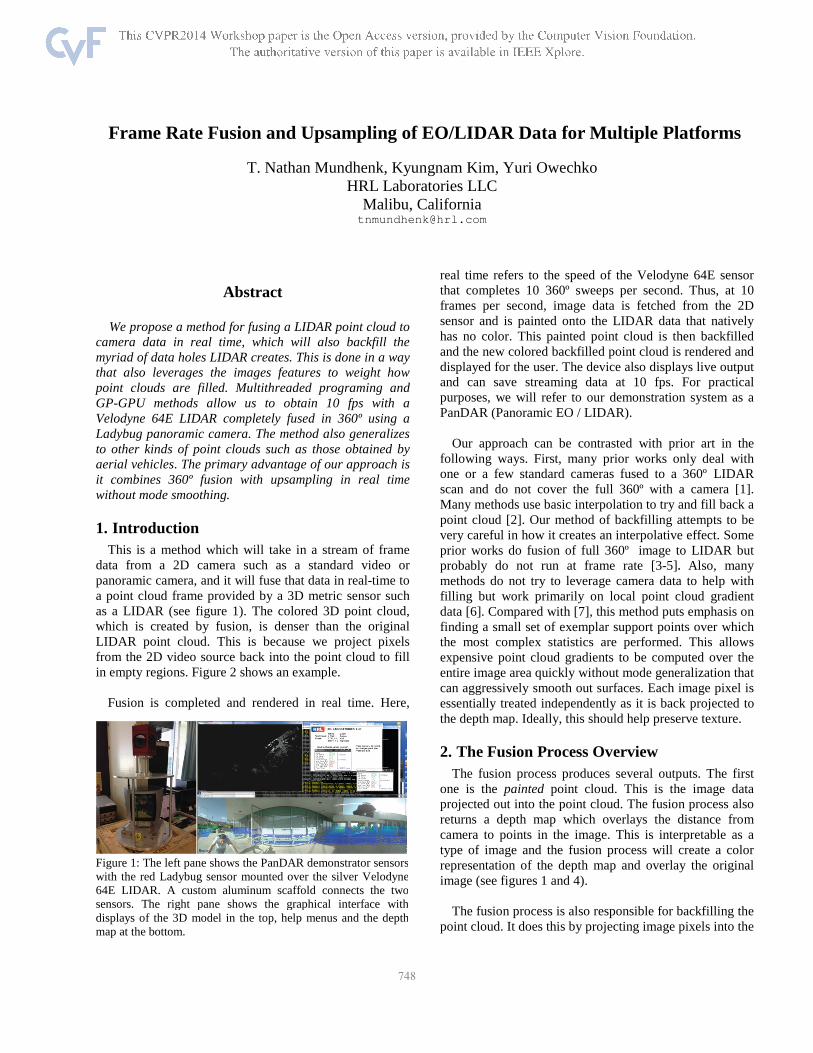
Figure 1: The left pane shows the PanDAR demonstrator sensors with the red Ladybug sensor mounted over the silver Velodyne 64E LIDAR. A custom aluminum scaffold connects the two sensors. The right pane shows the graphical interface with displays of the 3D model in the top, help menus and the depth map at the bottom. .

748

4322

point cloud where points do not exist. Thus, it deduces new points from the existing point cloud and input image. It attempts to determine where projected points in fact belong since some holes in a point cloud belong there. This is done in part by restricting backfilled window sizes, selecting reasonable support points and checking the sanity of obtained gradients.

The fusion process attains frame rate speed through the

usage of a variety of methods of parallel processing. These include the usage of SSE intrinsics, parallel threading, and GPU processing. The style of parallel processing used depends on what is most prudent for the given component of the fusion process. To reduce the wait time as each frame arrives, the fusion process creates and maintains threaded service pools that are responsible for different computations. For instance, if we have eight computing cores on a machine, the fusion process will create eight point cloud painting thread threads. When a new point cloud needs to be painted, the process manager will transfer the bare point cloud and image data to the waiting threads.

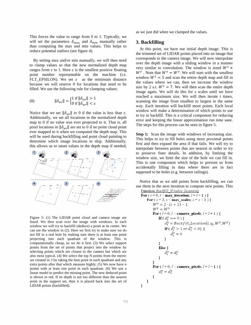
The fusion process can be thought of as being comprised of a set of major steps (seen in figure 3). (1) Depth Map Projection – In this step, the point cloud is

projected onto the camera. (2) Depth Normalization – This is a step that normalizes

the distances of point cloud points to the camera. (3) Backfilling – Given the point cloud and how it is

projected into the camera, this creates a much more dense new point cloud.

(4) Point Cloud Painting – This is the inverse of the Depth Map Projection step. Here we project point clouds that we had prior projected into the image back out into a new point cloud.

2.1. Calibration Notes

The cameras are calibrated with LIDAR in different ways depending on the camera model. If we have a standard EO camera, then we use EPnP [8] to derive a 4 x 4 perspective transformation matrix. For the Ladybug camera, we use their provided panoramic image. This has the shortcoming of inaccurate seams that are created where each camera image overlaps. However, the Ladybug driver can provide this image very quickly. So, it is convenient to use. Each pixel in the panoramic image corresponds linearly to the azimuth and elevation from the camera to the location in space. For example, pixels in image column 0 all project to 0º azimuth from the camera. If the image has 2048 columns, then all pixels in column 1024 are at azimuth 180º. Rows of the image are also similarly linear. It is convenient to solve projection by triangulation because of this. Given the azimuth, elevation from the Ladybug camera to a LIDAR point in space (��, ��), the center image pixels (�� , �) and pixels per degree (� , ) we get the coordinates from a LIDAR

Figure 3: This is a block diagram for the general fusion process. The details for each of the blue boxes can be seen in the block diagrams located in their sections. Flow of data is shown with dashed lines and flow of instructions is shown with a solid arrow.

Figure 2: The figure shows a room rendered at frame rate with our method. The left image is the raw point cloud (enhanced to make points easier to see). The middle image is the fused point cloud and the right image is the backfilled and fused cloud. The user can toggle through different modes in the interface to show the plain unfused point cloud, the fused and painted, but unfilled cloud or the fused and filled cloud. This is rendered and updated to the screen in real time and can be manipulated to show different views using a mouse.

749

4323

point to the panoramic image as: (1) � � � �� � �� �(�� � �� ∙ �) (2) � � � �� � �� �(� � �� ∙ ) 2.2. Depth Map Projection

Depth map projection takes in the point cloud and projects it into the 2D image. The camera model is flexible and allows for many different types of images and cameras to be used. The implementation is made more efficient through parallelization of workload using multiple work threads. Given N input points in a point cloud and M threads, each thread will process approximately � �⁄ points. Some threads may process a few more or less than the other threads if N does not evenly divide by M.

The depth projection process will first check to see if it

has any work. If there are no elements in the point cloud that are ready, it will simply return. Otherwise, it will translate each point in the point cloud to the input image. Given M threads ���, �� …�� and N points �!�, !� …!" each point contains a Euclidian coordinate in x,y,z space #$% , &% , '%( ∈ !% for any point �. Points can contain other properties as well, but for now we are just interested in the coordinates. We want to find the location in an image at some pixel location u,v where !%projects to. Depending on the type of camera model we have, we will do this differently.

A thread will take a slice of work based on the formula:

(3) ��*�� � � ∙ +,-.

(4) /01 � � ∙ +,-2�. � 1

The value of start is the index for the first point P we

will operate on while end is the index of the last point we will operate on. That means the thread will operate on /01 � ��*�� number of points. The value tid is the thread id (the subscripted value of t). As an example, if we have 12 threads, tid will be an integer between 0 and 11.

For each point in a thread, we will now translate that

point into camera coordinates, create a depth map of the distance to the point and handle the odd situation where points may overlap in camera coordinates. This last item can happen because the LIDAR and camera are not exactly aligned, so they have a slightly different perspective. Points in the LIDAR may occlude one another from the perspective of the camera. So we need to have some way of dealing with these occlusions when they are encountered.

2.3. Computing the Depth Map

Next we compute the depth map. This yields the distance of a point in the point cloud mapped to the pixel location u,v. The depth map will be used in back filling and later to project the filled/painted depth map into a new painted point cloud.

Let 4� be the distance from the camera to the point

mapped to pixel u,v. More than one point might map to the same pixel. We will handle that one later. For now, we compute this depending on the camera model. For a standard camera, we compute:

(5) 4� � 5$�� � &�� � '�� We know the u,v for this pixel already because we just computed it using projection transformation. We also take a copy of the $� , &� , '� which we got from computing u and v. We now need to handle the case in which more than one point maps to a pixel. We do this by taking the minimum value. This is the point closest to the camera:

(6) 4� � 64�7 if4�7 ; 4�4�otherwise

2.4. Depth Normalization

Given the depth map, normalize the values to range from 0 to 1. Also, store the normalizing value so that we can denormalize the depth map at a later point. The essential reason for doing this is that is makes the math easier to deal with. The general form of normalization we use is:

(7) ‖4�‖ � DEFGDHIJDHKLGDHIJ

Figure 4: The image shows the depth map superimposed over an input image section from the Ladybug camera. The colors correspond to the distance from the camera to the point.

750

4324

This forces the value to range from 0 to 1. Typically, we will set the parameters 4�MN and 4�," manually rather than computing the max and min values. This helps to reduce potential outliers (see figure 4).

By setting max and/or min manually, we will then need to clamp values so that the new normalized depth map ranges from O to 1. Here O is the smallest positive floating point number representable on the machine (i.e. FLT_EPSILON). We set O as the minimum distance because we will reserve 0 for locations that need to be filled. We use the following rule for clamping values:

(8) ‖4�‖ � 61if‖4�‖ P 10if‖4�‖ ; O

Notice that we set ‖4�‖ to 0 if the value is less than O. Additionally, we set all locations in the normalized depth map to 0 if no value was ever projected to it. That is, all pixel locations in ‖4�‖ are set to 0 if no point cloud point ever mapped to it when we computed the depth map. This will be used during backfilling and point cloud painting to determine which image locations to skip. Additionally, this allows us to unset values in the depth map if needed;

as we just did when we clamped the values.

3. Backfilling At this point, we have our initial depth image. This is

the trimmed set of LIDAR points placed into an image that corresponds to the camera image. We will now interpolate over the depth image with a sliding window in a manner very similar to convolution. The window is sized RN SRT . Note that RN � RT. We will start with the smallest window RN � 5 and scan the entire depth map and fill in the values where we can, then we increase the window size by 2 s.t. RN � 7. We will then scan the entire depth image again. We will do this for s scales until we have reached a maximum size. We will then iterate t times, scanning the image from smallest to largest in the same way. Each iteration will backfill more points. Each local window will make a determination of which points to use to try to backfill. This is a critical component for reducing error and keeping the linear approximation run time sane. The steps for this process can be seen in figure 5. Step 1: Scan the image with windows of increasing size. This helps to try to fill holes using more proximal points first and then expand the area if that fails. We will try to interpolate between points that are nearest in order to try to preserve finer details. In addition, by limiting the window size, we limit the size of the hole we can fill in. This is one component which helps to prevent us from accidentally filling in data where there are in fact supposed to be holes (e.g. between railings).

Notice that as we add points from backfilling, we can

use them in the next iteration to compute new points. This

Figure 5: (1) The LIDAR point cloud and camera image are fused. We then scan over the image with windows. In each window we will try to backfill (deduce) a point at its center. We can see the window in (2). Here we first try to make sure we do not fill in a real hole by making sure there is at least one point projecting into each quadrant of the window. This is computationally cheap, so we do it first. (3) We select support points from the set of points that project into the window by selecting points which are closest to the camera but which are also most typical. (4) We select the top N points from the metric we created in 3 by taking the best point in each quadrant and any extra points after that which measure highly. (5) We now have npoints with at least one point in each quadrant. (6) We use a linear model to predict the missing point. The new deduced point is shown in red. If its depth is not too different than the nearest point in the support set, then it is placed back into the set of LIDAR points (backfilled).

751

4325

allows us to span some larger gaps by filling them in. Also notice that we check to make sure new depth points are within the normalized space. This is an easy way to get rid of possible outlier error points.

The function Backfill_Location will scan over points in the window sized RN S RTat the location l. It will apply the support point selection process and execute linear approximation to estimate the missing point location. These steps help to reduce errors such as pass through (figure 6) and noise replication/amplification. The function Backfill_Location goes through the following steps: Step 2: Are there enough points within the window to make a linear fit and is there one point in each quadrant? If not, return. Support points help to make sure we do not build a shelf of points out from a ledge. A hole must be surrounded on all sides in order to be filled. Step 3: Compute goodness for each point in the window.

This is derived as a combination of the distance of the point from the camera and its similarity to other points in the window. Let n be the number of points that project into this window. We will want to find a goodness for each point i of the n points. The first element of goodness is similarity. So, we define feature responses W�� W� given m number of features. Each F is a measure of a feature such as pixel image location, color, intensity etc. The feature dissimilarity of point at i, to all other points at j in the window s.t.X ≠ Z and points i and j project into the window we write as:

(9) Μ, � ∑ ]^_`,IG_`,abc2⋯2^_H,IG_H,abcJae`"

As the point at i becomes more like all other points Μ, approaches 0. So, if this number is high, it means that this point is very different from the other points in the window. For speed, our implementation only uses RGB color values and the location of the point as features (i.e. {r,g,b,x,y}). However, other features could also be used. By inputting location as a feature, this will tend to favor points that are proximal to each other.

Next, we take the distance measure of point i from the camera as:

(10) Δ, � 1,g ∙ h

Here, h is a normalizing constant to make the distance from camera metric range similar to features. However, if both feature and distances are normalized between 0 and 1, this can be set to √j. The idea here is to favor points closer to the device. This rule is most useful if there is a preponderance of similar looking points at very different distances.

The goodness score for the point at i in the window is then:

(11) k, � 5Μ,� � Δ,�

Now we can do the next steps: Step 4: Sort points in the window by their score G, take

Figure 6: On the left we can see an area of the roof top not filled correctly when we do not select support points but instead use all the points in the window. The points estimated in this case are placed half way between the roof and the base ledge. This is because the roof occludes the base ledge in that area of the camera view. Support point selection prevents us from using points in the wall behind the roof and gives a more correct output. As an additional note, the trees appear to retain their texture, which is desirable.

752

4326

the lowest scoring (top N) points per quadrant

Sorting is done using a static memory non-recurrent quick sort that can run on GPU [9]. In our method, we select the point with highest density in each quadrant. This guarantees that we have one point in each quadrant if it exists. We add points using these steps:

(1) Find the highest density point in quadrant 1, add to

support point list. (2) Find the highest density point in quadrant 2, add to

support point list. (3) Find the highest density point in quadrant 3, add to

support point list. (4) Find the highest density point in quadrant 4, add to

support point list. (5) If we desire to add more than 4 points, add N-4 points

not already added with the highest density

We now have our final set of support points. We have two last steps before returning a new filled point. Step 5: Linear approximate 1lg from support points

This is done using any number of linear solvers for k number of values where the matrix is over determined. The current implementation uses singular value decomposition (SVD) to solve a linear system. Since we only input 5 support points, this keeps SVD sane in computation time.

What we want is the distance to some point i given its

location u,v:

(12) 1mlg � no � �l ∙ n� � �l ∙ n� We can solve this since we know the u and v from the support points as well as their distance d. This is done by solving a standard over determined matrix in least squares for the weights:

(13) p 1 �� ��⋯ ⋯ ⋯1 �" �"q pnon�n�

q � p1�o⋯1"oq

Note that it is easier to solve this by using image coordinates relative to the center of the current window coordinate.

Step 6: Check that 1mlg is in bounds. If not, set 1lgto 0 and return. Otherwise return 1mlg.

We want to make sure that the new estimated point is not too far from the nearest point in our windowed point set. This prevents points from draping across regions they should not. For instance, it prevents the top of trees from connecting to the ground in an overhead view. We compute it as:

(14) 4�MN- � 4"rMsrt+ ∙ u1 � v ∙ wx� y

(15) 4�,"- � 4"rMsrt+ u1 � v ∙ wx� yz

Here 4"rMsrt+ is the distance to the point closest to the camera within the kernel window boundaries. This is drawn from all the points in the kernel region, not just the support points. �{ is the width of the kernel. Generally, this is in pixels. v is an adjustable parameter we set constant in our implementation. The higher this number is, the further away points can be from the nearest point. In practice it appears that this number can be hand tuned and then left alone. Thus, there appears to be a good fixed setting for many sensors.

Figure 8: The top table shows the number of points in the new back filled point cloud given an initial set of 791,000 points. The bottom table shows the amount of time it took to process fusion and backfilling on the data. From the data, it appears that twoiterations and a kernel from 9x9 to 17x17 is optimal for the number of points filled and time taken.

Figure 7: The left most figure shows the image of a top of a building from the CSUAV data set of Columbus Ohio (same building seen in figure 6). The middle image shows the image fused to the raw point cloud. The image on the right shows the image fused in a backfilled point cloud. The colors in the fused only point cloud are correct, but it can be hard to make out features given its sparseness. The back filled cloud is much easier to interpret and appears to be generally correct.

753

4327

The goodness rule is applied very simply. If the new

distance we derived is not within bounds, we will set it to 0 and return:

(16) 1mlg � |0if1mlg P 4�MN- 0if1mlg ; 4�,"-

The backfilled point cloud is returned from normalized distances by inverting equation (7) and denormalizing the distance.

Backfilling is essentially a convolutional like

computation. This makes it trivial to port it to GP-GPU processing whereby each pixel that is projected back into the point cloud can be computed independently in parallel. Depending on the GPU used, this gives it an approximately 5x speed up over conventional CPU processing and allows frame rate computation.

Figure 9: This is a single frame from the PanDAR device. The top frame shows the panoramic image input. The unfilled cloud is created by fusing the image to the raw point cloud. Next to it is the backfilled point cloud. The lower left image shows the original point cloud in white and the new filled in points in red. In this instance, 138,907 new points are created which up samples the cloud by just over 3.5x. 78% of these new points are less than 6.25 cm from the original point. 3D Images in this figure were rendered with CloudCompare.

754

4328

4. Experimental Results

4.1. Backfilling Standard Camera Model and Aerial Data

Depending on the size of kernels used and the number of iterations, more points are filled in a given scene, but will also take more time. In general, the minimum set up will return about three times more points than were in the original cloud. For aerial data experiments, we use the public Columbus Surrogate Unmanned Aerial Vehicle (CSUAV) data set [10]. Figure 7 shows a breakdown of the amount of time taken to fill in the point cloud. This is the cloud seen at close up on a single building figure 8. In general, there is a diminishing return with the number of iterations for filling. For CSUAV data, and qualitatively for PanDAR data, two iterations seem sufficient.

With kernel size selection, there is an upper size for

filling in a reasonable working LIDAR scan that will nonetheless ignore large data holes. So for example, if the LIDAR scan beam can be observed spaced every 4 pixels when projected into the image, then a kernel of size 5 will sufficiently fill in the gaps between the returns. If one has an area with specular surfaces, the observed gap between the beams can be very large. It will take a much larger kernel to fill in the missed returns from mirrored windows or fountains. With the CSUAV data, a kernel sized from 9x9 to 17x17 seems enough to fill in general gaps between the LIDAR scans. Much larger kernels can be used, but kernel sizes larger than 51x51 pixels begin to show noticeable artifacts. As such, the method cannot be used in its current form to fill in very large holes in the LIDAR scan. Areas that are occluded from the camera in the point cloud are not filled in. This is because we are projecting pixel data from the camera back into the point cloud.

Since the PanDAR fusion/backfilling and the UAV

fusion/backfilling use the same process, some of the lessons can be applied from one to the other. However, the PanDAR system processes point clouds much faster due to the fact that the PanDAR point cloud has fewer points and the operable region of interest is very constrained in the Ladybug image.

4.2. Panoramic Camera Model Results

The current implementation runs on a Dell Precision T7600 Workstation with a GeForce 690 GTX GPU, 64 Gb RAM and two six core 2.0 GHz Xeon E5 processors. To get frame rate performance out of the fusion process when running the PanDAR demonstrator, we limit the maximum kernel size to 7x7. As processors increase in efficiency and/or the code is improved, we should be able to increase this number and get more filling than we are getting

currently since we can increase the size of kernels. Figure 9 shows an example of a fused and backfilled point cloud rendered at 10 fps on the PanDAR demonstrator. Much of the noise in the PanDAR image that can be seen is due to the usage of a first generation Velodyne 64E. This is seen as jagged edges on what are in actuality smooth surfaces.

5. Conclusion At frame rate, we can fuse EO from a 360º Ladybug

sensor to a Velodyne 64E LIDAR sensor as well as backfill the point cloud to increase detail. The same fusion approach can be used on other types of cameras by defining a different camera model. Qualitatively, backfilled locations look free of error and texture is at least partially preserved.

References [1] G. Zhao, X. Xiao, and J. Yuan, "Fusion of Velodyne and

camera data for scene parsing " presented at the 15th International Conference on Information Fusion (FUSION), 2012

[2] J. R. Arrowsmith, C. Crosby, and J. Conner. (2006). Notes on Lidar interpolation. Available: http://lidar.asu.edu/KnowledgeBase/Notes_on_Lidar_interpolation.pdf

[3] R. Wang, F. Ferrie, and J. Macfarlane, "Automatic Registration of Mobile LiDAR and Spherical Panoramas," presented at the CVPR Workshop on Point Cloud Processing in Computer Vision, 2012.

[4] F. M. Mirzaei, D. G. Kottas, and S. I. Roumeliotis, "3D Lidar-Camera Intrinsic and Extrinsic Calibration: Observability Analysis and Analytical Least Squares-based Initialization," International Journal of Robotics Research, vol. In-Press, 2012.

[5] R. Wang, J. Bach, J. Macfarlane, and F. Ferrie, "A New Upsampling Method for Mobile LiDAR Data," in IEEE Workshop on Applications of Computer Vision (WACV), 2012.

[6] H. Badino, D. Huber, Y. Park, and T. Kanade, "Fast and Accurate Computation of Surface Normals from Range Images," presented at the 2011 IEEE International Conference on Robotics and Automation., Shanghai, China., 2011.

[7] J. D. a. S. Thrun, "An Application of Markov Random Fields to Range Sensing," presented at the NIPS, 2005.

[8] F. Moreno-Noguer, V. Lepetit, and P. Fua, "Accurate Non-Iterative O(n) Solution to the PnP Problem.," in IEEE International Conference on Computer Vision (ICCV), Rio de Janeiro, Brazil, 2007.

[9] D. R. Finley. (2007). Optimized QuickSort — C Implementation (Non-Recursive). Available: http://alienryderflex.com/quicksort/

[10] Columbus Surrogate Unmanned Aerial Vehicle (CSUAV) Dataset. Available: https://www.sdms.afrl.af.mil/index.php?collection=csuav

755