Lidar Based Off-road Negative Obstacle Detection and Analysis

Jacoby Larson and Mohan TrivediComputer Vision and Robotics Research Laboratory

University of California, San DiegoLa Jolla, California 92093-0434

jacoby.larson@navy.mil, mtrivedi@ucsd.edu

Abstract— In order for an autonomous unmanned groundvehicle (UGV) to drive in off-road terrain at high speeds, itmust analyze and understand its surrounding terrain in real-time: it must know where it intends to go, where are the hazards,and many details of the topography of the terrain. Muchresearch has been done in the way of obstacle avoidance, terrainclassification, and path planning, but still so few UGV systemscan accurately traverse off-road environments at high speedsautonomously. One of the most dangerous hazards found off-road are negative obstacles, mainly because they are so difficultto detect. We present algorithms that analyze the terrain usinga point cloud produced by a 3D laser range finder, then attemptto classify the negative obstacles using both a geometry-basedmethod we call the Negative Obstacle DetectoR (NODR) as wellas a support vector machine (SVM) algorithm. The terrain isanalyzed with respect to a large UGV with the sensor mountedup high as well as a small UGV with the sensor mounted lowto the ground.

I. INTRODUCTION

Unmanned vehicle navigation and obstacle avoidance hashad major breakthroughs in the last few years, showing thata vehicle can drive without human intervention in highlycontrolled desert and urban environments such as was provedin the Defense Advanced Research Projects Agency (DARPA)Grand Challenge and DARPA Urban Challenge. In addition,the Jet Propulsion Laboratory (JPL) has shown that unmannedvehicles “Spirit” and “Opportunity” can navigate through theharshest of off-road environments, Mars, albeit at a very slowpace. Yet UGV autonomy has been difficult to incorporateinto a rugged off-road real-time scenario. This technologylag is in large part due to lack of real-time autonomousoff-road traversability analysis for unmanned ground vehi-cles (UGV), including negative obstacle detection at greatdistances. Military applications for UGVs such as resupply,casualty evacuation, surveillance, and reconnaissance mustaccommodate off-road terrain based on the warfighting areasin which the US military is currently involved. Accuratelyrepresenting off-road terrain and analyzing it in real-time is achallenge for most UGV robotic systems and the majority ofUGVs operate at slow speeds over relatively flat terrain. Arecent report by SSC Pacific [1] concerning the mobility ofUGVs for dismounted marines provides a survey and analysisof current robotic technologies and concludes that there aresignificant weaknesses in each system, especially in the areaof mobility in the face of hazardous terrain. This report alsoidentifies that NATO’s vital gaps are ”moving in all terrainwith tactical behavior in nearly all weather conditions” .

There are significant improvements that need to be made inautonomous obstacle detection and avoidance before thosehigher mission-oriented tasks can be accomplished in theareas of the world the US military is currently fighting, anddetecting negative obstacles is an important aspect of theproblems that need to be addressed.

II. RELATED RESEARCH

Negative obstacles are difficult to detect, especially at longranges, but methods used have included searching for negativeslopes that are too steep or gaps in data that exceed a distancethreshold followed by a drop in elevation or a steep uphillslope [2], [3], [4]. JPL uses both a column detector for gapsthat exceed a width and height threshold with a region sizefilter to eliminate negative obstacles that are too short aswell as a unidirectional elevation difference detector. In [5],[6], ray tracing is perfomed from the current position of thelaser and context-based labeling from occlusions from theground or positive obstacles are considered while detectingnegative obstacles. JPL also has presented a novel methodfor detecting negative obstacles using thermal signature fornight-time detection [7].

Other methods include using aerial image and lidar data,which has been demonstrated [8] to do negative obstacledetection as well, which can detect the bottom of the negativeobstacle, which is not always the case from the perspectiveof a ground robot.

This work can be beneficial to the general intelligent vehiclepublic, and can be combined with such computer vision safetysystems as have been described in [9], [10].

III. APPROACH

A. Sensor and Platform Selection

The negative obstacle detection methods and software thathave been developed for this research are designed for anunmanned ground vehicle using a 3D lidar. This research wasconducted to fit both a large and a small unmanned groundvehicle platform, using a large and a small 3D lidar. Theintended large platform is a Max ATV (Figure 2). It is asix-wheel skid-steer all terrain vehicle with dimensions oflength 2.6m, width 1.5m, and height, including a roll bar,of 1.7m. The 3D lidar used on the large UGV platform is aVelodyne HDL-64E. This lidar system provides readings ofrange and intensity out to a distance of 120 meters with 80%reflectivity, providing 100,000 data points with 360 degrees

2011 14th International IEEE Conference onIntelligent Transportation SystemsWashington, DC, USA. October 5-7, 2011

U.S. Government work not protected by U.S.copyright

192

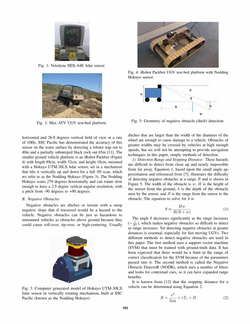
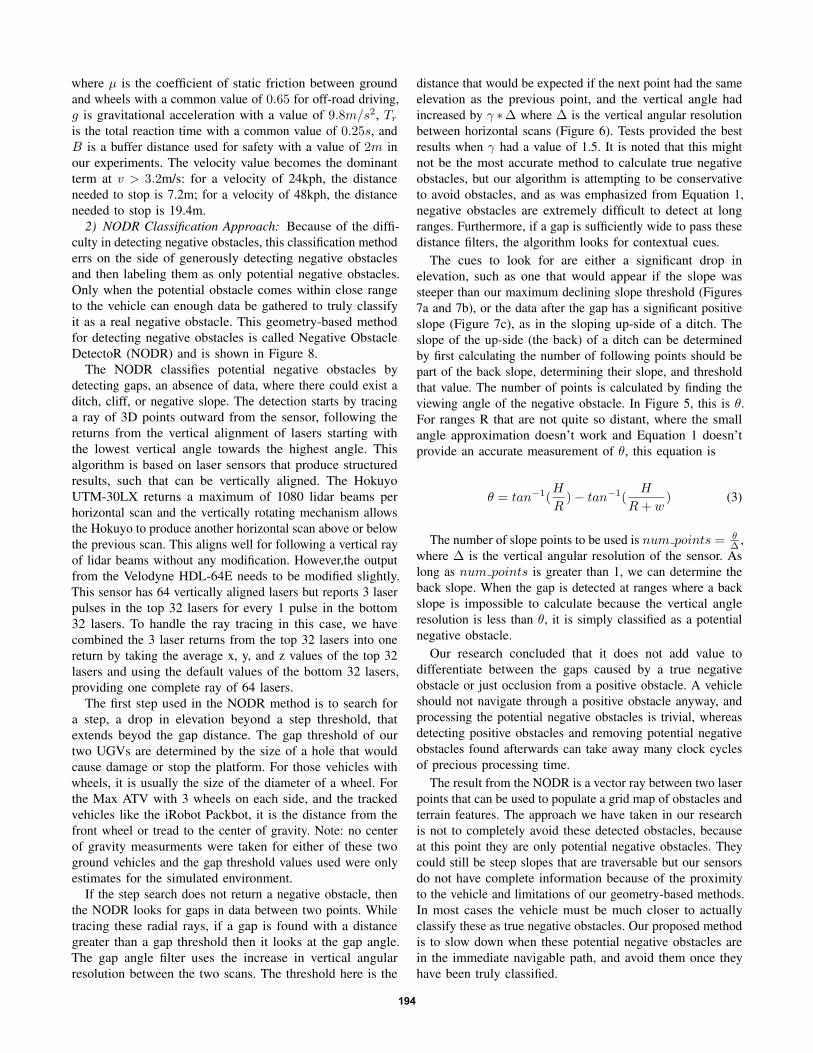
Fig. 1: Velodyne HDL-64E lidar sensor

Fig. 2: Max ATV UGV test-bed platform

horizontal and 26.8 degrees vertical field of view at a rateof 10Hz. SSC Pacific has demonstrated the accuracy of thissensor on the water surface by detecting a lobster trap out to40m and a partially submerged black rock out 65m [11]. Thesmaller ground vehicle platform is an iRobot Packbot (Figure4) with length 89cm, width 52cm, and height 18cm, mountedwith a Hokuyo UTM-30LX lidar sensor, set in a mechanismthat tilts it vertically up and down for a full 3D scan, whichwe refer to as the Nodding Hokuyo (Figure 3). The NoddingHokuyo scans 270 degrees horizontally and can rotate slowenough to have a 2.5 degree vertical angular resolution, witha pitch from -90 degrees to +90 degrees.

B. Negative Obstacles

Negative obstacles are ditches or terrain with a steepnegative slope that if traversed would be a hazard to thevehicle. Negative obstacles can be just as hazardous tounmanned vehicles as obstacles above ground because theycould cause roll-over, tip-over, or high-centering. Usually

Fig. 3: Computer generated model of Hokuyo UTM-30LXlidar sensor in vertically rotating mechanism, built at SSCPacific (known as the Nodding Hokuyo)

Fig. 4: iRobot Packbot UGV test-bed platform with NoddingHokuyo sensor

Fig. 5: Geometry of negative obstacle (ditch) detection

ditches that are larger than the width of the diameter of thewheel are enough to cause damage to a vehicle. Obstacles ofgreater widths may be crossed by vehicles at high enoughspeeds, but we will not be attempting to provide navigationtechniques in this paper, simply methods of detection.

1) Detection Range and Stopping Distance: These hazardsare difficult to detect from close up and nearly impossiblefrom far away. Equation 1, based upon the small angle ap-proximation and referenced from [7], illustrates the difficultyof detecting negative obstacles at a range R and is shown inFigure 5. The width of the obstacle is w, H is the height ofthe sensor from the ground, h is the depth of the obstacleseen by the sensor, and R is the range from the sensor to theobstacle. The equation to solve for θ is

θ ≈ Hw

R(R+ w)(1)

The angle θ decreases significantly as the range increases(∼ 1

R2 ), which makes negative obstacles so difficult to detectas range increases. Yet detecting negative obstacles at greaterdistances is essential, especially for fast moving UGVs. Twodifferent methods to detect negative obstacles are used inthis paper. The first method uses a support vector machine(SVM) that must be trained with ground-truth data. It hasbeen expected that there would be a limit in the range ofcorrect classification for the SVM because of the parameterspassed into it. The second method is called the NegativeObstacle DetectoR (NODR), which uses a number of filtersand looks for contextual cues, so it can have expanded rangebenefits.

It is known from [12] that the stopping distance for avehicle can be determined using Equation 2.

R =v2

2µg+ vTr +B (2)

193

where µ is the coefficient of static friction between groundand wheels with a common value of 0.65 for off-road driving,g is gravitational acceleration with a value of 9.8m/s2, Tris the total reaction time with a common value of 0.25s, andB is a buffer distance used for safety with a value of 2m inour experiments. The velocity value becomes the dominantterm at v > 3.2m/s: for a velocity of 24kph, the distanceneeded to stop is 7.2m; for a velocity of 48kph, the distanceneeded to stop is 19.4m.

2) NODR Classification Approach: Because of the diffi-culty in detecting negative obstacles, this classification methoderrs on the side of generously detecting negative obstaclesand then labeling them as only potential negative obstacles.Only when the potential obstacle comes within close rangeto the vehicle can enough data be gathered to truly classifyit as a real negative obstacle. This geometry-based methodfor detecting negative obstacles is called Negative ObstacleDetectoR (NODR) and is shown in Figure 8.

The NODR classifies potential negative obstacles bydetecting gaps, an absence of data, where there could exist aditch, cliff, or negative slope. The detection starts by tracinga ray of 3D points outward from the sensor, following thereturns from the vertical alignment of lasers starting withthe lowest vertical angle towards the highest angle. Thisalgorithm is based on laser sensors that produce structuredresults, such that can be vertically aligned. The HokuyoUTM-30LX returns a maximum of 1080 lidar beams perhorizontal scan and the vertically rotating mechanism allowsthe Hokuyo to produce another horizontal scan above or belowthe previous scan. This aligns well for following a vertical rayof lidar beams without any modification. However,the outputfrom the Velodyne HDL-64E needs to be modified slightly.This sensor has 64 vertically aligned lasers but reports 3 laserpulses in the top 32 lasers for every 1 pulse in the bottom32 lasers. To handle the ray tracing in this case, we havecombined the 3 laser returns from the top 32 lasers into onereturn by taking the average x, y, and z values of the top 32lasers and using the default values of the bottom 32 lasers,providing one complete ray of 64 lasers.

The first step used in the NODR method is to search fora step, a drop in elevation beyond a step threshold, thatextends beyod the gap distance. The gap threshold of ourtwo UGVs are determined by the size of a hole that wouldcause damage or stop the platform. For those vehicles withwheels, it is usually the size of the diameter of a wheel. Forthe Max ATV with 3 wheels on each side, and the trackedvehicles like the iRobot Packbot, it is the distance from thefront wheel or tread to the center of gravity. Note: no centerof gravity measurments were taken for either of these twoground vehicles and the gap threshold values used were onlyestimates for the simulated environment.

If the step search does not return a negative obstacle, thenthe NODR looks for gaps in data between two points. Whiletracing these radial rays, if a gap is found with a distancegreater than a gap threshold then it looks at the gap angle.The gap angle filter uses the increase in vertical angularresolution between the two scans. The threshold here is the

distance that would be expected if the next point had the sameelevation as the previous point, and the vertical angle hadincreased by γ ∗∆ where ∆ is the vertical angular resolutionbetween horizontal scans (Figure 6). Tests provided the bestresults when γ had a value of 1.5. It is noted that this mightnot be the most accurate method to calculate true negativeobstacles, but our algorithm is attempting to be conservativeto avoid obstacles, and as was emphasized from Equation 1,negative obstacles are extremely difficult to detect at longranges. Furthermore, if a gap is sufficiently wide to pass thesedistance filters, the algorithm looks for contextual cues.

The cues to look for are either a significant drop inelevation, such as one that would appear if the slope wassteeper than our maximum declining slope threshold (Figures7a and 7b), or the data after the gap has a significant positiveslope (Figure 7c), as in the sloping up-side of a ditch. Theslope of the up-side (the back) of a ditch can be determinedby first calculating the number of following points should bepart of the back slope, determining their slope, and thresholdthat value. The number of points is calculated by finding theviewing angle of the negative obstacle. In Figure 5, this is θ.For ranges R that are not quite so distant, where the smallangle approximation doesn’t work and Equation 1 doesn’tprovide an accurate measurement of θ, this equation is

θ = tan−1(H

R) − tan−1(

H

R+ w) (3)

The number of slope points to be used is num points = θ∆ ,

where ∆ is the vertical angular resolution of the sensor. Aslong as num points is greater than 1, we can determine theback slope. When the gap is detected at ranges where a backslope is impossible to calculate because the vertical angleresolution is less than θ, it is simply classified as a potentialnegative obstacle.

Our research concluded that it does not add value todifferentiate between the gaps caused by a true negativeobstacle or just occlusion from a positive obstacle. A vehicleshould not navigate through a positive obstacle anyway, andprocessing the potential negative obstacles is trivial, whereasdetecting positive obstacles and removing potential negativeobstacles found afterwards can take away many clock cyclesof precious processing time.

The result from the NODR is a vector ray between two laserpoints that can be used to populate a grid map of obstacles andterrain features. The approach we have taken in our researchis not to completely avoid these detected obstacles, becauseat this point they are only potential negative obstacles. Theycould still be steep slopes that are traversable but our sensorsdo not have complete information because of the proximityto the vehicle and limitations of our geometry-based methods.In most cases the vehicle must be much closer to actuallyclassify these as true negative obstacles. Our proposed methodis to slow down when these potential negative obstacles arein the immediate navigable path, and avoid them once theyhave been truly classified.

194

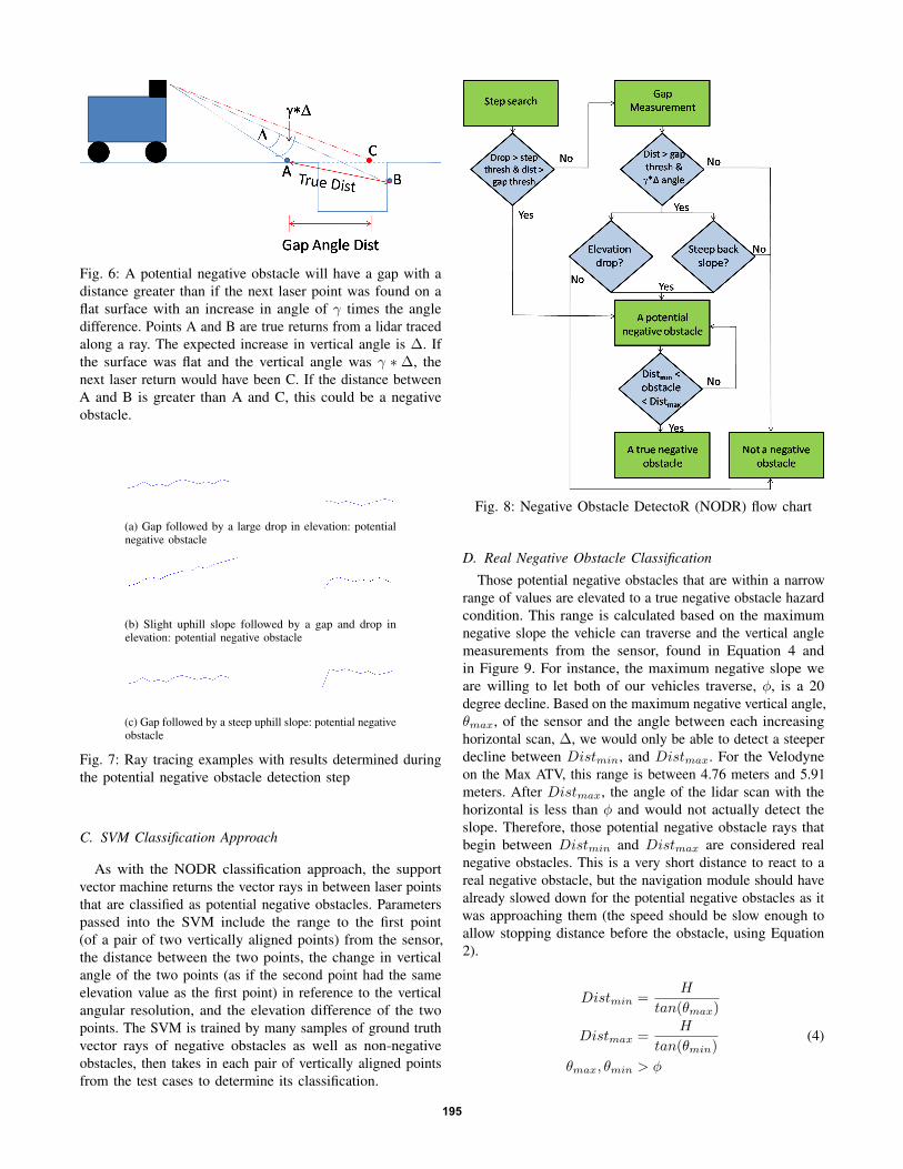
Fig. 6: A potential negative obstacle will have a gap with adistance greater than if the next laser point was found on aflat surface with an increase in angle of γ times the angledifference. Points A and B are true returns from a lidar tracedalong a ray. The expected increase in vertical angle is ∆. Ifthe surface was flat and the vertical angle was γ ∗ ∆, thenext laser return would have been C. If the distance betweenA and B is greater than A and C, this could be a negativeobstacle.

(a) Gap followed by a large drop in elevation: potentialnegative obstacle

(b) Slight uphill slope followed by a gap and drop inelevation: potential negative obstacle

(c) Gap followed by a steep uphill slope: potential negativeobstacle

Fig. 7: Ray tracing examples with results determined duringthe potential negative obstacle detection step

C. SVM Classification Approach

As with the NODR classification approach, the supportvector machine returns the vector rays in between laser pointsthat are classified as potential negative obstacles. Parameterspassed into the SVM include the range to the first point(of a pair of two vertically aligned points) from the sensor,the distance between the two points, the change in verticalangle of the two points (as if the second point had the sameelevation value as the first point) in reference to the verticalangular resolution, and the elevation difference of the twopoints. The SVM is trained by many samples of ground truthvector rays of negative obstacles as well as non-negativeobstacles, then takes in each pair of vertically aligned pointsfrom the test cases to determine its classification.

Fig. 8: Negative Obstacle DetectoR (NODR) flow chart

D. Real Negative Obstacle Classification

Those potential negative obstacles that are within a narrowrange of values are elevated to a true negative obstacle hazardcondition. This range is calculated based on the maximumnegative slope the vehicle can traverse and the vertical anglemeasurements from the sensor, found in Equation 4 andin Figure 9. For instance, the maximum negative slope weare willing to let both of our vehicles traverse, φ, is a 20degree decline. Based on the maximum negative vertical angle,θmax, of the sensor and the angle between each increasinghorizontal scan, ∆, we would only be able to detect a steeperdecline between Distmin, and Distmax. For the Velodyneon the Max ATV, this range is between 4.76 meters and 5.91meters. After Distmax, the angle of the lidar scan with thehorizontal is less than φ and would not actually detect theslope. Therefore, those potential negative obstacle rays thatbegin between Distmin and Distmax are considered realnegative obstacles. This is a very short distance to react to areal negative obstacle, but the navigation module should havealready slowed down for the potential negative obstacles as itwas approaching them (the speed should be slow enough toallow stopping distance before the obstacle, using Equation2).

Distmin =H

tan(θmax)

Distmax =H

tan(θmin)(4)

θmax, θmin > φ

195

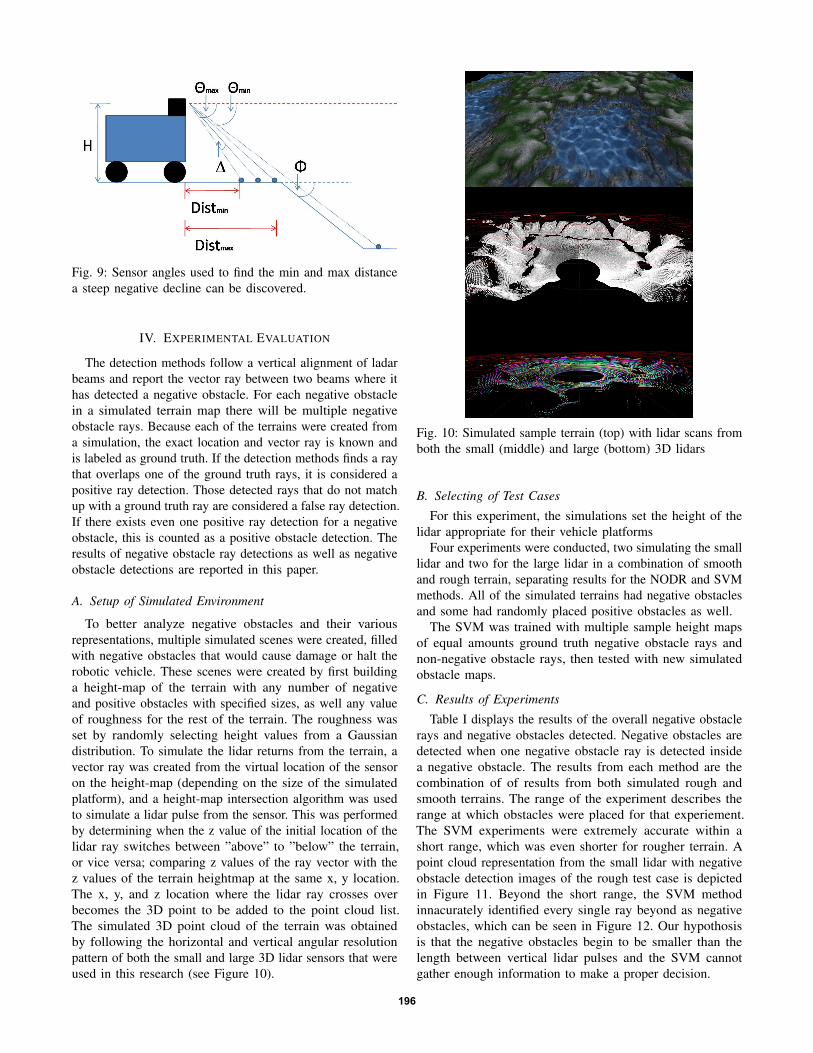
Fig. 9: Sensor angles used to find the min and max distancea steep negative decline can be discovered.

IV. EXPERIMENTAL EVALUATION

The detection methods follow a vertical alignment of ladarbeams and report the vector ray between two beams where ithas detected a negative obstacle. For each negative obstaclein a simulated terrain map there will be multiple negativeobstacle rays. Because each of the terrains were created froma simulation, the exact location and vector ray is known andis labeled as ground truth. If the detection methods finds a raythat overlaps one of the ground truth rays, it is considered apositive ray detection. Those detected rays that do not matchup with a ground truth ray are considered a false ray detection.If there exists even one positive ray detection for a negativeobstacle, this is counted as a positive obstacle detection. Theresults of negative obstacle ray detections as well as negativeobstacle detections are reported in this paper.

A. Setup of Simulated Environment

To better analyze negative obstacles and their variousrepresentations, multiple simulated scenes were created, filledwith negative obstacles that would cause damage or halt therobotic vehicle. These scenes were created by first buildinga height-map of the terrain with any number of negativeand positive obstacles with specified sizes, as well any valueof roughness for the rest of the terrain. The roughness wasset by randomly selecting height values from a Gaussiandistribution. To simulate the lidar returns from the terrain, avector ray was created from the virtual location of the sensoron the height-map (depending on the size of the simulatedplatform), and a height-map intersection algorithm was usedto simulate a lidar pulse from the sensor. This was performedby determining when the z value of the initial location of thelidar ray switches between ”above” to ”below” the terrain,or vice versa; comparing z values of the ray vector with thez values of the terrain heightmap at the same x, y location.The x, y, and z location where the lidar ray crosses overbecomes the 3D point to be added to the point cloud list.The simulated 3D point cloud of the terrain was obtainedby following the horizontal and vertical angular resolutionpattern of both the small and large 3D lidar sensors that wereused in this research (see Figure 10).

Fig. 10: Simulated sample terrain (top) with lidar scans fromboth the small (middle) and large (bottom) 3D lidars

B. Selecting of Test Cases

For this experiment, the simulations set the height of thelidar appropriate for their vehicle platforms

Four experiments were conducted, two simulating the smalllidar and two for the large lidar in a combination of smoothand rough terrain, separating results for the NODR and SVMmethods. All of the simulated terrains had negative obstaclesand some had randomly placed positive obstacles as well.

The SVM was trained with multiple sample height mapsof equal amounts ground truth negative obstacle rays andnon-negative obstacle rays, then tested with new simulatedobstacle maps.

C. Results of Experiments

Table I displays the results of the overall negative obstaclerays and negative obstacles detected. Negative obstacles aredetected when one negative obstacle ray is detected insidea negative obstacle. The results from each method are thecombination of of results from both simulated rough andsmooth terrains. The range of the experiment describes therange at which obstacles were placed for that experiement.The SVM experiments were extremely accurate within ashort range, which was even shorter for rougher terrain. Apoint cloud representation from the small lidar with negativeobstacle detection images of the rough test case is depictedin Figure 11. Beyond the short range, the SVM methodinnacurately identified every single ray beyond as negativeobstacles, which can be seen in Figure 12. Our hypothosisis that the negative obstacles begin to be smaller than thelength between vertical lidar pulses and the SVM cannotgather enough information to make a proper decision.

196

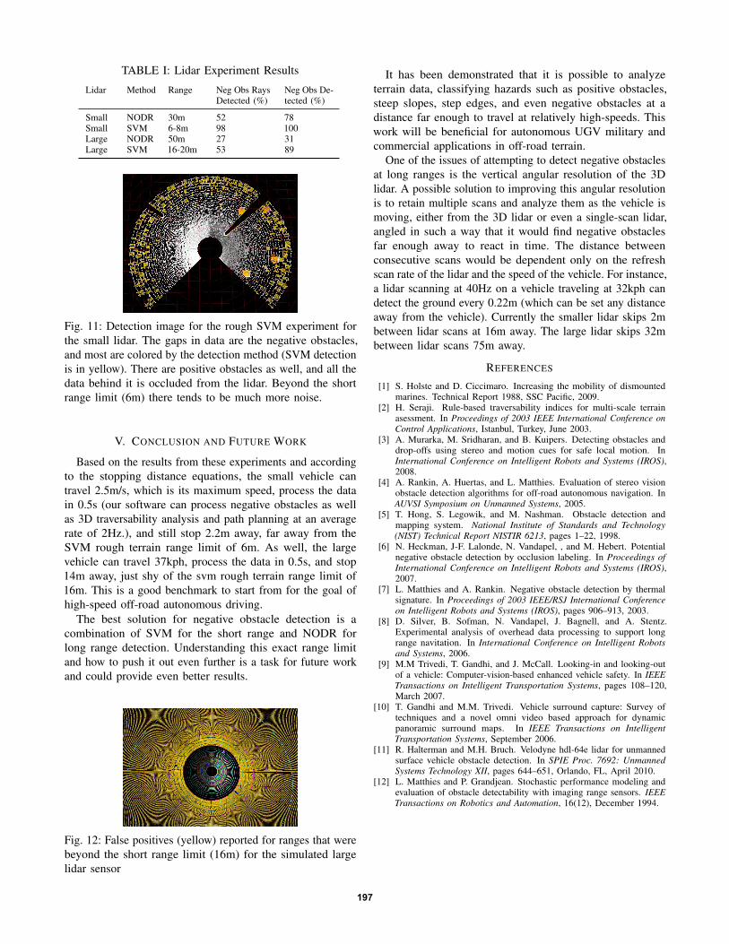
TABLE I: Lidar Experiment Results

Lidar Method Range Neg Obs RaysDetected (%)

Neg Obs De-tected (%)

Small NODR 30m 52 78Small SVM 6-8m 98 100Large NODR 50m 27 31Large SVM 16-20m 53 89

Fig. 11: Detection image for the rough SVM experiment forthe small lidar. The gaps in data are the negative obstacles,and most are colored by the detection method (SVM detectionis in yellow). There are positive obstacles as well, and all thedata behind it is occluded from the lidar. Beyond the shortrange limit (6m) there tends to be much more noise.

V. CONCLUSION AND FUTURE WORK

Based on the results from these experiments and accordingto the stopping distance equations, the small vehicle cantravel 2.5m/s, which is its maximum speed, process the datain 0.5s (our software can process negative obstacles as wellas 3D traversability analysis and path planning at an averagerate of 2Hz.), and still stop 2.2m away, far away from theSVM rough terrain range limit of 6m. As well, the largevehicle can travel 37kph, process the data in 0.5s, and stop14m away, just shy of the svm rough terrain range limit of16m. This is a good benchmark to start from for the goal ofhigh-speed off-road autonomous driving.

The best solution for negative obstacle detection is acombination of SVM for the short range and NODR forlong range detection. Understanding this exact range limitand how to push it out even further is a task for future workand could provide even better results.

Fig. 12: False positives (yellow) reported for ranges that werebeyond the short range limit (16m) for the simulated largelidar sensor

It has been demonstrated that it is possible to analyzeterrain data, classifying hazards such as positive obstacles,steep slopes, step edges, and even negative obstacles at adistance far enough to travel at relatively high-speeds. Thiswork will be beneficial for autonomous UGV military andcommercial applications in off-road terrain.

One of the issues of attempting to detect negative obstaclesat long ranges is the vertical angular resolution of the 3Dlidar. A possible solution to improving this angular resolutionis to retain multiple scans and analyze them as the vehicle ismoving, either from the 3D lidar or even a single-scan lidar,angled in such a way that it would find negative obstaclesfar enough away to react in time. The distance betweenconsecutive scans would be dependent only on the refreshscan rate of the lidar and the speed of the vehicle. For instance,a lidar scanning at 40Hz on a vehicle traveling at 32kph candetect the ground every 0.22m (which can be set any distanceaway from the vehicle). Currently the smaller lidar skips 2mbetween lidar scans at 16m away. The large lidar skips 32mbetween lidar scans 75m away.

REFERENCES

[1] S. Holste and D. Ciccimaro. Increasing the mobility of dismountedmarines. Technical Report 1988, SSC Pacific, 2009.

[2] H. Seraji. Rule-based traversability indices for multi-scale terrainasessment. In Proceedings of 2003 IEEE International Conference onControl Applications, Istanbul, Turkey, June 2003.

[3] A. Murarka, M. Sridharan, and B. Kuipers. Detecting obstacles anddrop-offs using stereo and motion cues for safe local motion. InInternational Conference on Intelligent Robots and Systems (IROS),2008.

[4] A. Rankin, A. Huertas, and L. Matthies. Evaluation of stereo visionobstacle detection algorithms for off-road autonomous navigation. InAUVSI Symposium on Unmanned Systems, 2005.

[5] T. Hong, S. Legowik, and M. Nashman. Obstacle detection andmapping system. National Institute of Standards and Technology(NIST) Technical Report NISTIR 6213, pages 1–22, 1998.

[6] N. Heckman, J-F. Lalonde, N. Vandapel, , and M. Hebert. Potentialnegative obstacle detection by occlusion labeling. In Proceedings ofInternational Conference on Intelligent Robots and Systems (IROS),2007.

[7] L. Matthies and A. Rankin. Negative obstacle detection by thermalsignature. In Proceedings of 2003 IEEE/RSJ International Conferenceon Intelligent Robots and Systems (IROS), pages 906–913, 2003.

[8] D. Silver, B. Sofman, N. Vandapel, J. Bagnell, and A. Stentz.Experimental analysis of overhead data processing to support longrange navitation. In International Conference on Intelligent Robotsand Systems, 2006.

[9] M.M Trivedi, T. Gandhi, and J. McCall. Looking-in and looking-outof a vehicle: Computer-vision-based enhanced vehicle safety. In IEEETransactions on Intelligent Transportation Systems, pages 108–120,March 2007.

[10] T. Gandhi and M.M. Trivedi. Vehicle surround capture: Survey oftechniques and a novel omni video based approach for dynamicpanoramic surround maps. In IEEE Transactions on IntelligentTransportation Systems, September 2006.

[11] R. Halterman and M.H. Bruch. Velodyne hdl-64e lidar for unmannedsurface vehicle obstacle detection. In SPIE Proc. 7692: UnmannedSystems Technology XII, pages 644–651, Orlando, FL, April 2010.

[12] L. Matthies and P. Grandjean. Stochastic performance modeling andevaluation of obstacle detectability with imaging range sensors. IEEETransactions on Robotics and Automation, 16(12), December 1994.

197