Fractionalization of the electron

Claudio Chamon

PY 482 Lecture

Boston, April 4, 2013

Fractionalization in Polyacetelene

R. Jackiw and C. Rebbi, Phys Rev. D13, 3398 (1976)W. P. Su, J. R. Schrieffer and A. J. Heeger, PRL 42, 1698 (1979); PRB 22, 2099 (1980)

Fractionalization in Polyacetelene

A

R. Jackiw and C. Rebbi, Phys Rev. D13, 3398 (1976)W. P. Su, J. R. Schrieffer and A. J. Heeger, PRL 42, 1698 (1979); PRB 22, 2099 (1980)

Fractionalization in Polyacetelene

A

R. Jackiw and C. Rebbi, Phys Rev. D13, 3398 (1976)W. P. Su, J. R. Schrieffer and A. J. Heeger, PRL 42, 1698 (1979); PRB 22, 2099 (1980)

Fractionalization in Polyacetelene

A B

R. Jackiw and C. Rebbi, Phys Rev. D13, 3398 (1976)W. P. Su, J. R. Schrieffer and A. J. Heeger, PRL 42, 1698 (1979); PRB 22, 2099 (1980)

Fractionalization in Polyacetelene

A B

R. Jackiw and C. Rebbi, Phys Rev. D13, 3398 (1976)W. P. Su, J. R. Schrieffer and A. J. Heeger, PRL 42, 1698 (1979); PRB 22, 2099 (1980)

Fractionalization in Polyacetelene

A B

mid-gap StateAppeared

R. Jackiw and C. Rebbi, Phys Rev. D13, 3398 (1976)W. P. Su, J. R. Schrieffer and A. J. Heeger, PRL 42, 1698 (1979); PRB 22, 2099 (1980)

Counting the charge

Counting the charge

Counting the charge

Counting the charge

Counting the charge

Q = −1/2 Q = −1/2

Counting the charge

Q = −1/2 Q = −1/2

Fractional charge!

H Ψ(x) = 0

What are zero modes?

ΨE(x)←C−→ Ψ−E(x)

E

−E

Energy eigenvalues always come in pairs.So unpaired states are only allowed at

E = 0

H = p σ1 + ∆ σ2 =�

0 p− i∆p + i∆ 0

�

E = ±�

p2 + ∆2

Dirac Hamiltonian

E

−E2∆

H = p σ1 + ∆ σ2 =�

0 p− i∆p + i∆ 0

�

E = ±�

p2 + ∆2

Ψ−E(x) = σ3 ΨE(x)σ3 H σ3 = −H

Dirac Hamiltonian

E

−E2∆

Spatially dependent masses and zero modes

∆(x)+∆

−∆

�0 −i ∂

∂x − i∆(x)−i ∂

∂x + i∆(x) 0

� �u(x)v(x)

�= 0

R. Jackiw and C. Rebbi, Phys Rev. D13, 3398 (1976)

[−i σ1 ∂x + ∆(x) σ2] Ψ = E Ψ

E = 0⇒

E

−E2∆

∆(x)+∆

−∆

�0 −i ∂

∂x − i∆(x)−i ∂

∂x + i∆(x) 0

� �u(x)v(x)

�= 0

u(x) ∝ eR x0 dx� ∆(x�)

v(x) = 0

solution 1 solution 1I

u(x) = 0v(x) ∝ e−

R x0 dx� ∆(x�)

Zero mode is localized

E

−E2∆

∆(x)+∆

−∆

�0 −i ∂

∂x − i∆(x)−i ∂

∂x + i∆(x) 0

� �u(x)v(x)

�= 0

u(x) ∝ eR x0 dx� ∆(x�)

v(x) = 0

solution 1 solution 1I

u(x) = 0v(x) ∝ e−

R x0 dx� ∆(x�)

Zero mode is localized

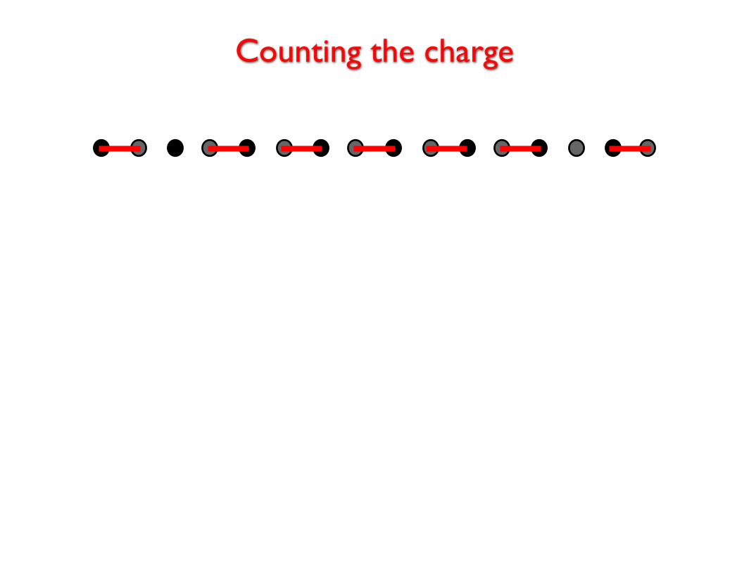
Counting the charge�

E

ρ(E, x) =�

E

ψ†E(x) ψE(x) = 1

�i.e.

�

E

�x|E� �E|x� = 1

�

Counting the charge

�

E

ρkink(E, x) =�

E

ρno kink(E, x)

�

E

ρ(E, x) =�

E

ψ†E(x) ψE(x) = 1

�i.e.

�

E

�x|E� �E|x� = 1

�

Counting the charge

�

E

ρkink(E, x) =�

E

ρno kink(E, x)

�

E �=0

ρkink(E, x) + |ψ0(x)|2 =�

E �=0

ρno kink(E, x)

�

E �=0

δρ(E, x) = −|ψ0(x)|2

�

E

ρ(E, x) =�

E

ψ†E(x) ψE(x) = 1

�i.e.

�

E

�x|E� �E|x� = 1

�

Counting the charge

�

E

ρkink(E, x) =�

E

ρno kink(E, x)

�

E �=0

ρkink(E, x) + |ψ0(x)|2 =�

E �=0

ρno kink(E, x)

�

E �=0

δρ(E, x) = −|ψ0(x)|2

2�

E<0

δρ(E, x) = −|ψ0(x)|2

�

E

ρ(E, x) =�

E

ψ†E(x) ψE(x) = 1

�i.e.

�

E

�x|E� �E|x� = 1

�

Counting the charge

�

E

ρkink(E, x) =�

E

ρno kink(E, x)

�

E �=0

ρkink(E, x) + |ψ0(x)|2 =�

E �=0

ρno kink(E, x)

�

E �=0

δρ(E, x) = −|ψ0(x)|2

2�

E<0

δρ(E, x) = −|ψ0(x)|2

δρ(x) = −12

|ψ0(x)|2 Q = −1/2

�

E

ρ(E, x) =�

E

ψ†E(x) ψE(x) = 1

�i.e.

�

E

�x|E� �E|x� = 1

�

Fractionalization in 2D Dirac fermion systems

C.-Y. Hou, C. Chamon, M. Mudry, PRL 98, 186809 (2007)

2D Dirac fermionsin condensed matter systems

Bipartite lattices A and B - hopping between these

A B

A

A

AB

B

BC

C

C

C

C

ALT - A ALT - B

KEKULE

The hopping texture leading to Δ:

Kekule Distortions:

C. Chamon, PRB 62, 2806 (2000)

A completed ‘flake’ of molecular graphene is shown in topographicform in Fig. 1b, demonstrating a perfect internal honeycomb latticeand discernable edge effects at the termination boundaries. The spec-trum shown in Fig. 1c was measured at the lattice C sites near thecentre of a lattice built using 271 COmolecules separated by a distanced5

ffiffiffi3

pa5 19.23 A. The spectra in all the figures show surface-state

conductance, ~g(E,r), where r denotes the measurement position.(Henceforth, ‘tilde’ quantities refer to continuum properties of theDirac fermions.) These spectra are measured by taking the ratio, gR,between the measured differential tunnelling conductance and thespatially averaged value acquired on clean Cu(111) (SupplementaryFig. 2). This normalization removes the featureless slope present in thebare Cu spectrum and cancels the effect of possible energy-dependenttunnellingmatrix elements thatmay vary between differentmicroscopetips. The jump in differential conductance at the two-dimensional bandedge, g2D5m*/pB2 5 1.585 eV21 nm22, additionally provides aquantitative calibration of the surface density of states (DOS) and isused to scale gR to meaningful units (Supplementary Information).The edge of the gap at the M point in momentum space (Fig. 1c) is

marked by the peak in conductance at EM52104meV. The Dirac

a

50d

Bt

E (m

eV)

˜

0

50A

–50–0.4 –0.2 0.2 0.40

↓⟩

↑⟩

↑⟩

↓⟩

sgn(sz)sgn(E)g (eV–1nm–2) ˜ ˜

b z (Å) 0.50

1.0c2 nm

K

0.5 ED

M ED

EM

–200 0 200

0.0

5 nm

g (e

V–1 n

m–2

)˜

V (mV)

Figure 1 | Dirac fermions in molecular graphene. a, Sequence of constant-current topographs during the assembly of a molecular graphene lattice(V5 10mV, I5 1 nA). b, Topograph of a molecular graphene latticecomposed of 149 CO molecules (lattice constant, d5 8.8 A). c, Spatiallyaveraged, normalized differential conductance spectrum, ~g(V) (solid line),measured on the top sites near the centre of quasi-neutral molecular graphene(d5 19.2 A), accompanied by a tight-binding DOS fit (dashed line) withhopping parameters t5 90meV and t95 16meV. Inset, resulting Dirac conerealized in reciprocal space (corresponding to fit parameters). The tight-binding spectrum is calculated by finding energy eigenvalues of a finitegraphene lattice with Lorentzian basis functions (to model the finite lifetimedue to scattering to bulk states and coupling to the two-dimensional continuumat the graphene edges, we used an electron self-energy S5C/2, where thelinewidth is C5 40meV from observed broadening of states near EF).d, Linearly dispersing quasi-particles revealed by the conductance spectra~g(~E,r), plotted individually for sublattice A (filled circles: pseudospin sz511/2, |"æ) and sublattice B (open circles: pseudospin sz521/2, |#æ), measured atlocations r illustrated in the inset. Points for |~E | = eVrms, where Vrms is themodulation voltage, are excluded from this plot because this instrumentalbroadening prohibits their accurate measurement.

P PNa

250 0.2

40 Å

b

ED

0

V (m

V)

EF

z (Å)

0

1.5

g

–2503000 x (Å)

0

c

1.0

1.5

0.5

–200 0 200 –200 0 200 –200 0 2000.0

V (mV) V (mV) V (mV)

˜

g (e

V–1 n

m–2

)˜

Figure 2 | Dirac point engineering in a p–n–p junction. Spectroscopicmeasurements made from a p–n–p lattice with alternating lattice spacings: dchanges abruptly from 17.8 to 20.4 A and then back again. a, Topograph of thep–n–p lattice. The conductance spectra were measured across the centre linemarked by the grey arrows. b, Intensity colour plot of the conductance spectra~g(V ,x), where x denotes the distance along the centre line. The white line is thelocus ofminima (theDirac points (ED)) in the conductance spectra. The dashedline marks the Fermi energy (EF). Illustrative Dirac cones are superimposed toshow the effective doping of each region. c, Spatially averaged, normalizedconductance spectra measured along the centre line (marked by arrows ina). The first spectrum (blue, left) was measured in the left-hand, p-type, region(d5 17.8 A), the second (orange, centre) was measured in the central, n-type,region (d5 20.4 A) and the third (blue, right) was measured in the right-hand,p-type, region (d5 17.8 A).

LETTER RESEARCH

1 5 M A R C H 2 0 1 2 | V O L 4 8 3 | N A T U R E | 3 0 7

Macmillan Publishers Limited. All rights reserved©2012ManoharanLab-MolecularGraphene-Nature-work1

“Molecular graphene”H. Manoharan ’s lab:K. K. Gomes et al., Nature 483, 306 (2012)

“Molecular graphene”H. Manoharan ’s lab:K. K. Gomes et al., Nature 483, 306 (2012)

t1=76 meV

t2=37 meV

tn1=20 meV

tn2= 8 meV

aAB

0

0

3

6

9

-3

-6

-9

-12

11

3-3-6-9-12 6 9 12

Kekulé

t1=76 meV

t2=37 meV

tn1=20 meV

tn2= 8 meV

aAB

t3=24 meV

0

0

3

6

9

-3

-6

-9

-12

11

3-3-6-9-12 6 9 12

Kekulé-vortex

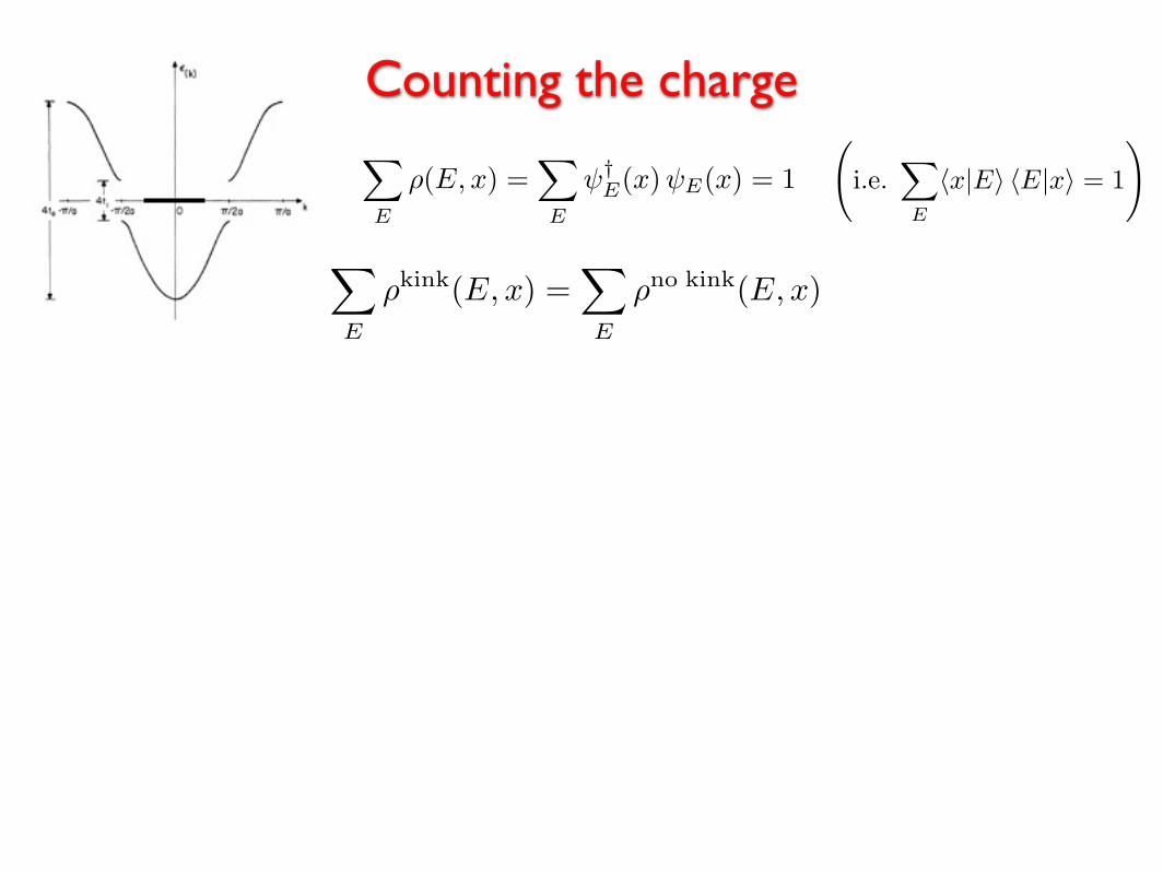
0.0

0.1

0.2

0.3

� 10

� 5

0

510

x� 10

� 5

05

10

y

A “picture” of a fractional charge