Ethnic Fractionalization, Governance and Loan Defaults in Africa

Svetlana Adrianova, University of Leicester

Badi H. Baltagi, Syracuse University and University of Leicester

Panicos Demetriades, University of Leicester

David Fielding, University of Otago

Working Paper No. 14/14

October 2014

ETHNIC FRACTIONALIZATION, GOVERNANCE

AND LOAN DEFAULTS IN AFRICA*

Svetlana Adrianova, University of Leicester

Badi H. Baltagi, Syracuse University and University of Leicester

Panicos Demetriades, University of Leicester

David Fielding, University of Otago

ABSTRACT. We present a theoretical model of moral hazard and adverse

selection in an imperfectly competitive loans market that is suitable for

application to Africa. The model allows for variation in both the level of

contract enforcement (depending on the quality of governance) and the

degree of market segmentation (depending on the level of ethnic

fractionalization). The model predicts a specific form of non-linearity in the

effects of these variables on the loan default rate. Empirical analysis using

African panel data for 111 individual banks in 29 countries over 2000-2008

provides strong evidence for these predictions. Our results have important

implications for the conditions under which policy reform will enhance

financial development.

KEYWORDS: Ethnic fractionalization, Governance, Financial development,

African Banks, Panel data.

JEL CLASSIFICATION: G21, O16

* We would like to acknowledge the support of ESRC-DFID grant number ES/J009067/1.

1

1. Introduction

In terms of financial development, Africa still lags behind other parts of the world.

African banks are deterred from lending in domestic markets by a lack of

creditworthy borrowers, and loan volumes are highly sensitive to default rates

(Adrianova et al., 2014). As a result, many African banks are excessively liquid and

channel an unusually large proportion of domestic savings abroad, although there is

substantial variation in banks’ default risk and asset structure, both within and

between countries (Honohan and Beck, 2007). At the same time, firm and household

surveys reveal endemic credit constraints. For this reason, understanding the

determinants of the rate of loan default is crucial in overcoming obstacles to

financial development in Africa. Our paper makes a first step in this direction by

providing both theory and evidence that shed new light on the factors behind the

high rate of loan default in many parts of Africa.

The focus of attention in both the theoretical and empirical parts of the paper

is on two key characteristics of the African banking sector. Firstly, there is great deal

of variability across Africa in terms of both the level of corruption and the quality of

contract enforcement. This variability is revealed in indices of the quality of

governance produced by organisations such as the World Bank, Transparency

International, and the Bureau van Dijk. Daumont et al. (2004) argue that weak

contract enforcement in Africa is due to a number of factors, including excessively

2

time-consuming and unwieldy legal procedures, high litigation costs, a lack of

appropriately qualified judges, and inadequacies in the cadastral system that inhibit

the identification of collateral property. The large variation in the magnitude of these

problems across Africa suggests that they may help explain the observed variation in

the incidence of loan default. Secondly, many African counties are characterized by a

high level of ethnic fractionalization (Easterly and Levine, 1997). A lack of trust

between different ethnic groups is likely to generate high inter-ethnic transactions

costs, which will lead to a high level of market segmentation (Aker et al., 2010;

Robinson, 2013). Existing studies of ethnic market segmentation have not focused

explicitly on financial markets, but there is no reason to suppose that financial

markets are any less susceptible to this problem than others. Even in countries with

a large banking sector, ethnic fractionalization is likely to create monopolistic

competition, because banks are differentiated by the ethnicity of their staff. African

banks are therefore likely to face unusually inelastic demand curves.

The theoretical section of the paper develops a model of loan default which

emphasizes the importance of imperfect competition and the quality of governance.

This model features both adverse selection and moral hazard, problems which are

exacerbated when market segmentation is more pronounced or when the quality of

contract enforcement is poor. Unsurprisingly, the theory predicts that high loan

default rates are more likely when there is greater market segmentation or when

3

contract enforcement is weak. But the model also produces some less obvious

predictions about non-linearities in these effects that arise from the interaction of

the market segmentation and contract enforcement problems. Improvements in the

quality of contract enforcement will reduce loan default rates only in certain

situations: specifically, when the contract enforcement problem is initially neither

much more severe nor much less severe than the market segmentation problem.

The theory can help explain why in some circumstances improvements in

enforcement quality have a large effect on loan default rates, but in other

circumstances there may be little or no effect. The empirical section of the paper

tests the predictions of the theoretical model using a panel data set on loan default

rates faced by individual African banks. In the empirical model, market segmentation

is interpreted in terms of ethnic fractionalization and contract enforcement is

interpreted in terms of the quality of governance as measured by the World Bank’s

World Governance Indicators. We find strong evidence to support the predictions of

the theoretical model, which has important implications for financial development

policy.

2. Theory

Our starting point is a Hotelling (1929) ‘linear city’ model that embodies a degree of

product differentiation between banks whose financial services are imperfectly

4

substitutable.1 There are three different types of entrepreneur who seek a loan of

one dollar in order to undertake an investment project: ‘honest’ borrowers (in

proportion ), ‘dishonest’ borrowers (in proportion ) and ‘opportunistic’ borrowers

(in proportion , with + + = 1). The honest type of borrower has an investment

project with a return of R dollars, and this borrower always repays the loan. The

opportunistic type of borrower has the same investment project (with a return R),

but can choose whether to repay or default on the loan. The dishonest type of

borrower has a project with rate of return equal to zero, and this borrower will

always default on the loan. The borrower’s type is private information, but the

proportions , and are publicly known.

1 Some of the features of our model are shared with other models that extend the credit

rationing theory of Stiglitz and Weiss (1981). For example, Besanko and Thakor (1987),

Petersen and Rajan (1995) and Hoff and Stiglitz (1998) develop theories of adverse selection

and /or moral hazard in a monopolistic competition setting. However, the banks in these

models have market power because of features such as increasing returns to scale, not

product differentiation. Villas-Boas and Schmidt-Mohr (1999) and Hauswald and Marquez

(2006) do present models that allow for product differentiation, but these models focus on

adverse selection rather than moral hazard, and do not allow for the variation in the quality

of contract enforcement that is central to our model. The model presented here is an

extension of the one in Andrianova et al. (2014), and, unlike that model, incorporates

asymmetric information on both sides of the transaction.

5

All borrowers are uniformly distributed along a unit interval with a distribution

density equal to one. Each borrower can apply for a loan from at most one bank.

There are two banks, which are located at opposite ends of the interval. The banks

compete for loan contracts, with bank i (i ∈ A, B) setting its loan interest rate ri to

maximise its expected payoff. Applying for a loan is costly to a borrower because of

a ‘transportation’ cost of t dollars per unit of distance between the borrower and the

bank. One interpretation of the distance between the banks is that it represents an

ethnic difference. For example, each of the two banks could be associated with a

different tribe, with the customers coming from a variety of tribes that are culturally

closer either to one bank’s tribe or to the other’s. In this interpretation, t is a

measure of the cost that accompanies interactions with other tribes. In general, we

might expect t to be larger in countries that are more ethnically diverse and in

which the unit interval in the model represents a greater cultural divide. In this way,

t parameterizes the magnitude of the market segmentation problem discussed in

the introduction.

Each bank has sufficient funds to approve all loan applications (which is

consistent with the findings of Honohan and Beck, 2007). The banks differ in their

ability to gather and use information about an individual borrower’s characteristics.2

2 This assumption can be justified by noting that in the presence of ‘connected lending’

those banks with connections to the political (or industrial) elite may intentionally approve

6

Either bank can be of one of the two types: a ‘competent’ type with a screening

technology or an ‘incompetent’ type with no ability to screen borrowers. The bank is

competent with probability and incompetent with probability 1 − . The value of

is common knowledge, but only the bank itself knows which type it is. If the

borrower is opportunistic or dishonest, then with probability the screening

technology reveals this information. With probability 1 − the screening fails to

reveal any information. With slight abuse of notation, we assume that a -type bank

chooses whether to screen or not to screen, and then whether to refuse or not to

refuse applications from borrowers with a negative screening signal. Both banks

have access to a safe asset with a return equal to r0 (0 r0 R).

Loan contract enforcement is imperfect. When a loan has funded a project

with a return of R, default on the loan is penalized with probability ; the penalty is

equal to 1 + R dollars, of which the bank receives 1 + ri dollars. In other words, if

the bank is compensated then it receives the amount stipulated in the loan contract.

With probability 1 − no contract enforcement is possible and there is no penalty.

When the loan has funded a project with a zero return, no enforcement of the loan

contract is ever possible.

loans to politically connected borrowers regardless of any adverse information that is

available or can be gathered through screening.

7

The return on the investment is observable ex post and is non-falsifiable. All

players are risk-neutral. The timing of events is as follows:

(1) Bank i sets its lending rate ri.

(2) Each borrower chooses a bank to apply for a loan of one dollar.

(3) Facing a demand for loans equal to Di, bank i chooses whether to screen

all of its loan applications or not. This choice will depend on whether it is a -

type bank.

(4) Each bank chooses which applications to approve and which to decline.

(5) Honest and opportunistic borrowers with an approved loan invest the

money.

(6) An honest borrower repays the loan, a dishonest borrower defaults, and an

opportunistic borrower chooses whether to repay or to default.

(7) In the case of default, the banks seek compensation.

(8) Payoffs are realized.

Let q ∈ 0, 1 denote an opportunistic borrower’s decision whether to repay (q = 1)

or to default (q = 0). Let ∈ 0, 1 be a -type bank’s decision to screen, with = 1

in the case of screening. Let pj ∈ 0, 1, where j ∈ , 1 – , be a j -type bank’s

decision whether to approve all of its applications when there is no screening. Note

that if the transportation cost t is too high then no-one will want to apply for a loan.

8

Also, if the proportion of dishonest borrowers (1 – ) is negligible then a competent

bank will find it unprofitable to use the screening technology. In what follows, we

assume that t and are low enough so there is a market for loans and the

screening technology is relevant. Solving the model backwards for pooling equilibria,

we obtain the following result:

Proposition 1. There exist values , , and t so that for ≥ and t ≤ t , the

unique equilibrium of the model is:

(i) The low default equilibrium (LDE) with q = = 1p = 1, when ≥ .

(ii) The high default equilibrium (HDE) with q = 0 and = 1p = 1, when

≤ .

(iii) The no lending equilibrium (NLE) with q = = p = 1p = 0, when

.

More details are given in Appendix A. Intuitively, the NLE occurs when contract

enforcement is very weak. In such a situation, widespread default by opportunistic

and dishonest borrowers makes lending unprofitable for any screening technology.

Since we do observe some bank lending, even in countries with very weak

institutions, the NLE is probably of theoretical interest only. The LDE occurs when

there is a non-negligible proportion of dishonest borrowers but contract

9

enforcement is sufficiently good. The HDE occurs within an intermediate range of

contract enforcement parameter values, when opportunistic borrowers have no

incentive to repay (given relatively weak enforcement) but the banks nevertheless

find it profitable to screen and to lend to all borrowers for whom no negative signal

has been obtained. (This equilibrium requires contract enforcement not to be too

weak and default compensated often enough to make lending profitable.) Note that

for all equilibria, both banks set the same interest rate: rA = rB.

In Appendix A we derive an equation for which takes the following form:

1

1

ii A B

rr r r

R

, (1)

Equation (1) defines the minimal value of required for the market to be in the LDE:

below this value, the HDE will obtain. Appendix A also includes an equation for the

interest rate in the LDE:

01

11 1

i

rtr

(2)

Combining equations (1-2) we have:

10

011

1 1 1

rt

R

(3)

The two key country characteristics that we will be analyzing in the next section are

the quality of governance (interpreted in our theoretical model as ) and the

magnitude of ethnic fractionalization (which we interpret as a correlate of the

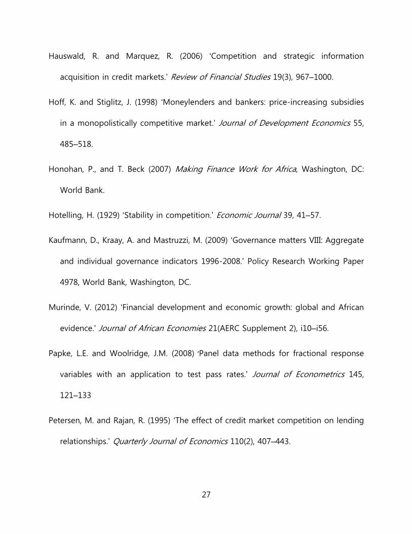
‘transportation’ cost t). Equation (3) implies that in (, t) space the LDE-HDE

boundary will be an upward-sloping line, as shown in Figure 1. Higher values of t

push up the boundary value of : a higher level of ‘transportation’ costs gives more

local monopoly power to the banks and pushes up the equilibrium interest rate; this

makes opportunistic borrowers more likely to default at the margin, so better

contract enforcement is required to maintain the LDE equilibrium.

Figure 1 exactly describes a country in which all investment projects yield the

same return R. In such a country, small changes in or t will have no effect on the

default rate unless the starting point is very close to the boundary line. If the

starting point is close to the boundary line, then a small change could take the

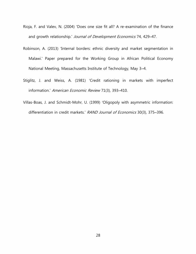
country across the line, with a very large change in the default rate. In reality,

however, different investors are likely to face different returns: for example, returns

could vary from one part of the country to another. If each bank is lending in a

variety of regional markets, each market with its own R-value, then a different

boundary line will be associated with each market. There will be a distribution of

11

boundary lines, as illustrated by the gray area in Figure 2. Outside of the gray area,

small changes in or t will still have no effect on the overall default rate for a bank,

but inside the area there will be some effect, as the boundary line is crossed for

some value of R. If the R-values are unimodally distributed, then the magnitude of

the effect of a small change in or t will be greater when the starting point is closer

to the modal boundary line (the black line in Figure 2). In other words, the response

of the overall default rate to a small change in or t will be smaller when the

starting point is further from the modal boundary line, i.e. when either is high and

t is low, or is low and t is high.

This brings us to a set of specific empirical predictions about the relationship

between the default rate, governance and ethnic fractionalization across countries

and over time. Firstly, as long as some countries in some time periods fall within the

gray area in Figure 2, we should see a negative correlation between the default rate

and (governance), since a higher value of moves a country upwards towards the

LDE space; we should see a positive correlation between the default rate and t

(ethnic fractionalization), since a higher value of t moves a country rightwards

towards the HDE space. These predictions are unremarkable, but we should also see

that the size of the effects is greater in countries / time periods where there is either

(i) relatively poor governance and relatively low fractionalization (the south-west of

Figure 2) or (ii) relatively good governance and relatively high fractionalization (the

12

north-east of Figure 2). To put it another way, the level of governance at which

changes in governance matter depends on the level of fractionalization: the higher

the level of fractionalization, the higher the level of governance at which there will

be the most sensitivity of the default rate. In the next section we test this prediction

using cross-country panel data.

3. Evidence

In this section we present tests of the predictions outlined above, using African

panel data for 111 individual banks in 29 countries over 2000-2008 to fit a model of

the loan default rate of each bank. Our predictions relate to the relationship

between the default rate which a bank faces and the conditions of the market in

which it operates, primarily the quality of governance and the level of ethnic

fractionalization in the country. Our three key empirical variables are as follows:

(i) The default rate for bank i in year y (defaultiy), measured as the ratio of impaired

loans to total loans. The loans data are collated from the Bankscope database

published by the Bureau van Dijk (https://bankscope.bvdinfo.com).

(ii) The quality of governance in each country j in year y, (governancejy), measured

as the first principal component of the following three variables in the World Bank’s

13

World Governance Indicators (WGI) database

(http://info.worldbank.org/governance/wgi/): control of corruption, rule of law and

regulatory quality. Control of corruption measures ‘the extent to which public power

is exercised for private gain, including both petty and grand forms of corruption, as

well as “capture” of the state by elites and private interests.’ Rule of law measures

‘the extent to which agents have confidence in and abide by the rules of society,

and in particular the quality of contract enforcement, property rights, the police, and

the courts, as well as the likelihood of crime and violence.’ Regulatory quality

measures ‘the ability of the government to formulate and implement sound policies

and regulations that permit and promote private sector development.’ Further

discussion of the construction of these variables appears in Kaufmann et al. (2009);

we interpret each of the variables as a measure of some of the factors driving the

probability () that a bank will be able to enforce a loan contract if necessary. The

variables are highly correlated in our sample, so it is not feasible to include more

than one of them in any one model.3 Nevertheless, we will also explore the

sensitivity of our results to the way in which is measured by comparing the results

3 The correlation coefficients are 0.93 for control of corruption and rule of law, 0.82 for

control of corruption and regulatory quality, and 0.86 for rule of law and regulatory quality.

The weights in the first principal component are almost uniform: 0.58 for control of

corruption, 0.59 for rule of law, and 0.56 for regulatory quality.

14

using the principal component with results using any one of the three individual

indicators instead.

(iii) The log of ethnic fractionalization in country j (ethnicj). This variable measures

ethnic diversity using a Herfindahl index: 2

11

k K

j jkkethnic s

ln , where jks

is the share of the k

th ethnic group in the total population of country j. Figures are

taken from Alesina et al. (2003). Countries with more fractionalization are expected

to have a higher financial transactions cost (t) on average.

Variables (i-iii) are the main variables of interest. However, our empirical model also

includes a number of control variables. Firstly, in the theoretical model in section 2

there are two types of bank (competent and not competent), with competent banks

facing a lower default rate because their screening is partially effective. In practice

there are likely to be a variety of banks with different levels of competence, and the

empirical model includes some bank characteristics that may be correlated with

competence. These characteristics are all measured using Bankscope data.

(iv) The age of bank i in year y, measured in years (ageiy), plus (ageiy)

2. Older banks

may have had time to acquire competence in the screening of customers, in which

case we would expect the default rate to be decreasing in age. On the other hand,

15

very new banks may have fewer informal connections with the political elite and

come under less pressure to issue loans to customers of dubious creditworthiness, in

which case we would expect the default rate to be increasing in age.

(v) The size of bank i in year y, measured by the logarithm of total bank assets

(assetsiy), where asset values are expressed in 2005 US dollars. There may be

economies of scale in screening, in which case the default rate should be decreasing

in bank size.

(vi) The share of the government in ownership of bank i in year y (government-

ownershipiy). Government-owned banks may make less effort to screen certain

customers, either because of political patronage or because the government wishes

to raise the volume of finance to investors, even at the expense of a high rate of

default. In this case, the default rate should be increasing in the government

ownership share.

In addition to these measures of bank-specific heterogeneity, the empirical model

also includes two additional country-specific variables.

(vii) The rate of growth of country j ’s GDP between year y – 1 and year y (growth-

ratejy), where GDP is measured in 2005 US dollars, as reported in the World Bank’s

16

World Development Indicators (http://data.worldbank.org/products/wdi). A higher

growth rate may be associated with a relative abundance of investment

opportunities and a lower overall default rate.

(viii) An indicator variable equal to one if country j is in North Africa and zero

otherwise (North-Africaj). The North African countries in our sample are Egypt,

Morocco and Tunisia. Data presented by Honohan and Beck (2007) indicate that the

banking sector in North Africa differs from that in Sub-Saharan Africa in a number of

key respects: North Africa has lower interest margins and wider access to financial

services, and more closely resembles the banking sector of OECD countries. The

North-Africa variable is intended to capture this heterogeneity.

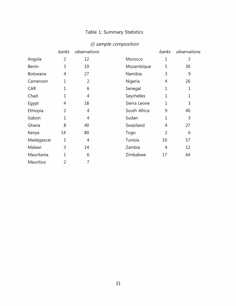
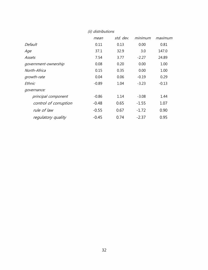
Summary statistics for the variables in the model are given in Table 1, which also

includes information about the distribution of banks across the 29 countries in our

sample. Missing observations for some banks in some years mean that we have an

unbalanced panel with 528 observations in total.

Our empirical model is designed to test hypotheses about the effect on

banks’ loan default rates of the quality of governance ( in the theoretical model,

governance in the empirics) and ethnic fractionalization (t in the theoretical model,

ethnic in the empirics). The theory implies that the effects will be non-linear, but first

17

of all we test whether governance and ethnic have any impact on default on

average. In order to do this, we note first of all that the dependent variable is

limited to the interval [0,1]. An appropriate estimator for this type of limited

dependent variable in a panel has been developed by Papke and Wooldridge (2008).

Our underlying model is assumed to be of the form:

1 2 3

2

3 5 6

7 8

-

- -

i y jy j iy

iy iy iy iy

jy j

governance ethnic age

E default F age assets government ownership i j

growth rate North Africa

, (4)

where F (.) is a cumulative density function, i is a bank random effect and y is a

year fixed effect. Following Papke and Wooldridge, we can estimate the

parameters in equation (4) using a pooled fractional logit (or probit) model of

default conditional on the eight explanatory variables plus the year fixed effects.

Consistent estimates of the parameters are obtained by maximizing the Bernoulli

log-likelihood function using a generalized linear model (GLM). The results below are

based on estimates using the GLM routine in Stata 12; we report results from the

logit version of the model, but the probit results are very similar.

18

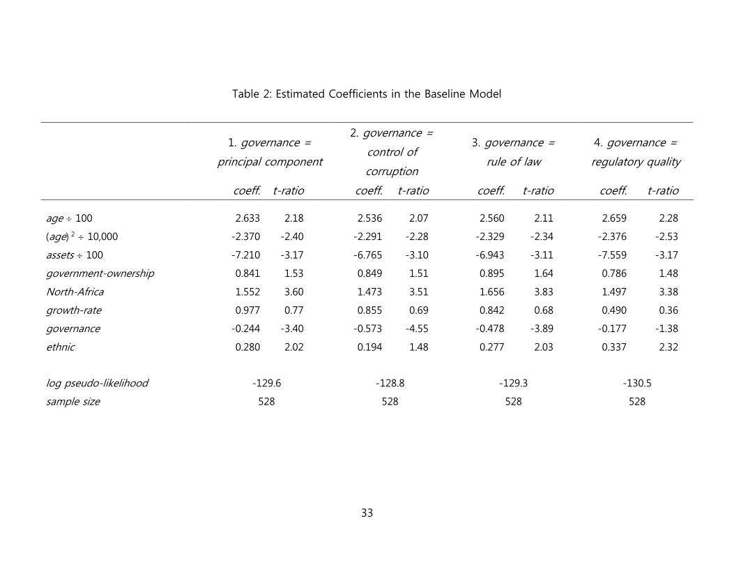
Table 2 reports the estimates of the parameters in equation (1).4 Column 1

of the table reports the parameter estimates in the model using the principal

component of the three WGI variables as the measure of governance, while columns

2-4 report the estimates using the individual WGI variables instead. The table also

includes the t-ratios for each parameter estimate, which are based on standard

errors clustered at the bank level. Note that with a fractional logit model, the

parameters in Table 2 are not equal to the partial derivatives of the default rate with

respect to each explanatory variable. Therefore, the parameters do not necessarily

indicate the relative importance of each variable for the default rate. Estimates of the

partial derivatives will be discussed later, and at this point we discuss only the signs

of the estimated effects.

In column 1, all of the estimated parameters are significantly different from

zero at the 5% level, except for those on government-ownership and growth-rate.

Ceteris paribus, smaller banks have significantly higher default rates than larger

ones, and middle-aged banks have significantly lower default rates than the

youngest and oldest banks: the quadratic term in age implies that the lowest default

rate is when age = 56 years. The non-monotonicity of the age effects may reflect

the fact that that there is more than one channel through which age affects defaults

4 The year fixed effects are jointly significant at the 1% level. They are not reported in the

table, but are available on request.

19

rates, as suggested above. Column 1 also shows that high default rates can be

mitigated by good governance and low ethnic fractionalization. Conditional on all of

these effects, North African banks have higher default rates than banks in Sub-

Saharan Africa: this effect was not anticipated and deserves further study. These

results are also feature of the models in columns 2-4, except that ethnic is not quite

significant when control of corruption is used to measure governance, and

regulatory quality is not quite significant when it is used to measure governance.

Nevertheless, the measures of governance and ethnic fractionalization are jointly

significant at the 5% level in all four versions of the Table 2 model, and the relevant

parameters have the expected signs in all cases. This suggests that our empirical

measures are relevant to the theoretical quantities and t, and we now proceed to

use these measures to test the predictions of the theoretical model about the

interaction between the effects of governance and ethnic fractionalization.

The theory predicts that the sensitivity of the default rate to governance and

ethnic fractionalization will be greater when either both of these characteristics are

relatively high or both of these characteristics are relatively low, in the north-east

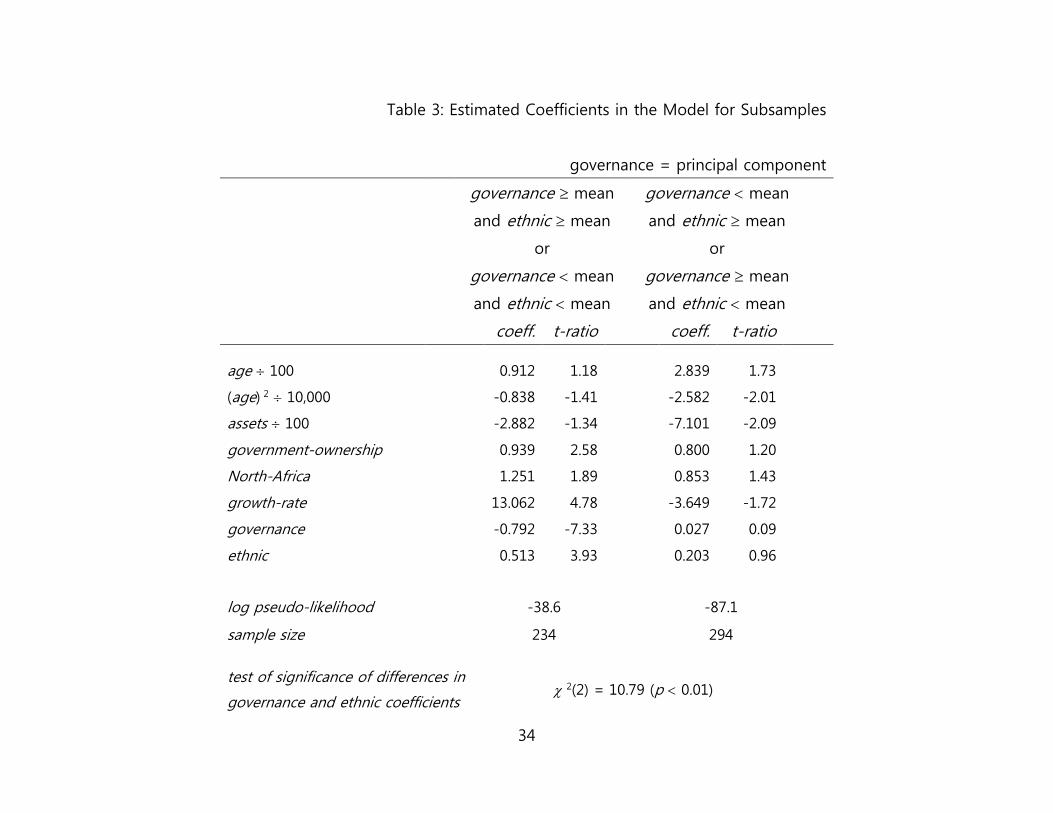
and south-west of Figure 2. Table 3 reports a test of this prediction based on

estimates of the parameters in equation (4) for two sub-samples: (i) observations for

which governance (as measured by the principal component) and ethnic are either

both above their sample mean values or both below their sample mean values; (ii)

20

observations for which either governance is above its sample mean value and ethnic

is below its sample mean value, or vice versa. If the prediction of the theory is

correct, then we can expect the absolute values of the 1 and 2 parameters to be

greater in (i) than in (ii). Table 3 shows that this is indeed the case; moreover, the

differences are jointly significant at the 1% level, and the 1 and 2 parameters in (ii)

are insignificantly different from zero. In other words, marginal changes in the

quality of governance (or in the level of ethnic fractionalization) have more impact

on the default rate when both are relatively high or both are relatively low, closer to

the dividing line in Figure 2.5

Given this significant difference, as predicted by the theoretical model, we can

try to estimate how default / governance and default / ethnic vary across different

points in Figure 2. In order to do this, we need to parameterize the interaction

between the governance and ethnic effects. With a large enough sample, one

possible approach would be to fit a model that included additional terms in

equation (4) of the form 10 governance governance – 12 ethnic

+ 11 ethnic governance – 12 ethnic . The parameters 10 and 11 would capture

5 Another striking feature of Table 3 is that the effect of growth-rate on default is

significantly positive in (i) and significantly negative in (ii). However, variations in the effect

of economic growth are not part of our theoretical predictions, so we do not pursue the

effect any further here.

21

the speed with which default / governance and default / ethnic fall as we move

away from the dividing line in Figure 2, and the parameter 12 would depend on the

slope of this line. However, the addition of these terms makes the argument of F (.)

in equation (4) non-linear, and, with just over 500 observations, estimates of 12 turn

out to be very imprecise. A slightly more restrictive alternative is to set 12 = 1 and

fit the following model:

1 2 3

2

3 5 6

7 8

9

10

-

- -

| |

|

i y jy j iy

iy iy iy

jy jiy

jy j

jy jy

governance ethnic age

age assets government ownership

growth rate North AfricaE default F

governance ethnic

governance governance eth

11

|

| |

,

j

j jy j

i j

nic

ethnic governance ethnic

(5)

Note that the means and standard deviations of the WGI principal component and

ethnic fractionalization variables in Table 1 are almost identical, so the results based

on equation (5) would not be substantially different if standardized measures of

these variables were used instead. Given the results in Table 3, we can expect that 1

0 2 and 10 0 11: larger absolute differences between the governance and

ethnic fractionalization variables diminish the absolute size of the effect of both

variables on the loan default rate.

22

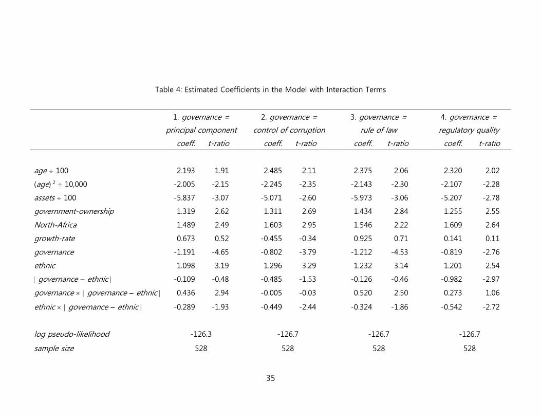
Column 1 of Table 4 shows the estimates of the parameters in equation (5),

along with the corresponding t-ratios. The signs of the four parameter estimates ( 1,

2, 10, 11) are consistent with our expectations, and other parameter estimates are

similar to those in column 1 of Table 2, except that the government-ownership

effect is somewhat larger and now significantly greater than zero: the default rates

of government-owned banks are higher than those of privately owned ones.

Columns 2-4 of Table 4 report results when the principal component is replaced by

one or other of the individual WGI variables. Here, the 1 and 2 estimates are

always significantly different from zero (which was not the case in Table 2), as are

the estimate of 10 when rule of law is used (column 3) and the estimates of 11

when control of corruption or regulatory quality are used (columns 2 and 4). All

significant parameter estimates have the expected sign. The log-likelihood in column

1 is higher than the log-likelihoods in the other columns, which indicates that using

a combination of the WGI variables to measure governance captures somewhat

more of the variation in default rates than using any one of the variables

individually.

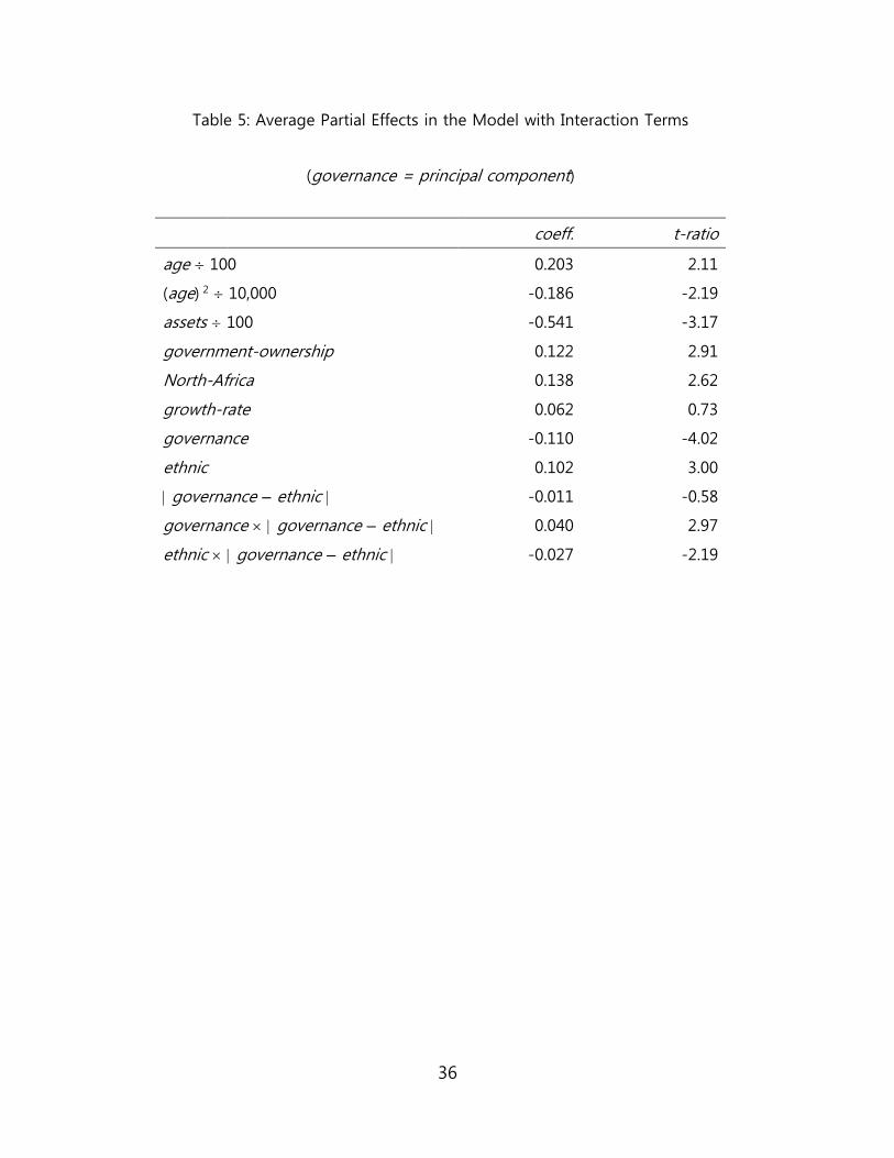
The results in column 1 of Table 4 can be used to calculate the average effect

of each variable on the default rate, i.e. n F ’ evaluated at the mean value of

default, n = 1,…, 11. These effects are reported in Table 5, along with the

corresponding t-ratios, which were computed using a bootstrap with 500

23

replications. This table shows that a 1% increase in the size of a bank (as measured

by its asset base) reduces the default rate by about half a percentage point, and that

a one percentage point increase in the share of the government in the bank’s

ownership increases the default rate by just over 0.1 percentage points. For a bank

of average age (37 years), an extra year of age also raises the default rate by just

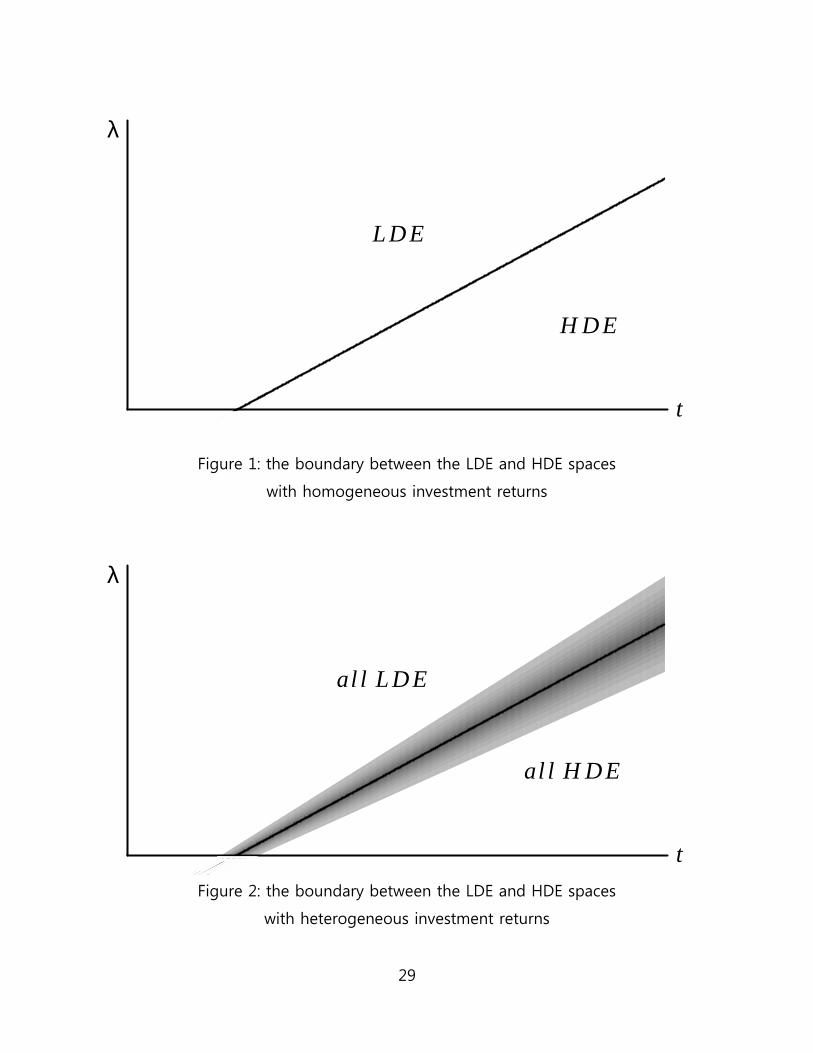
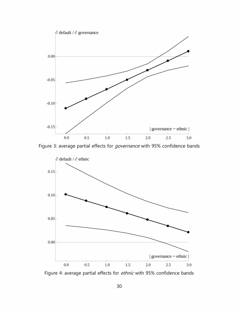
over 0.1 percentage points. In order to interpret the effects of governance and

ethnic fractionalization, note that the minimum value of governance

– ethnic is 0.01. At this value, when the governance – ethnic interaction terms are

negligible, a unit improvement in either governance or ethnic fractionalization (in

other words, a one standard deviation improvement, since the standard deviations

of these variables are both close to one) reduces the default rate by about ten

percentage points. Effects for larger values of governance – ethnic are shown in

Figures 3-4: at the mean value of governance – ethnic (about 1.5), the effects of

governance and ethnic fractionalization on the default rate are about half as large as

at the minimum value; at values of governance – ethnic greater than about 2.5 the

effects become insignificantly different from zero. Table 1 notes that the mean

default rate is 0.11 and the standard deviation is 0.13, so both the average effects of

governance and ethnic fractionalization and the sensitivity of these effects to

governance – ethnic are economically significant.

24

4. Discussion

The theoretical model presented in this paper shows that when a country’s banking

sector is characterized by market segmentation (which is one possible consequence

of ethnic fractionalization), adverse selection and moral hazard, improvements in the

quality of contract enforcement will sometimes – but not always – reduce the

incidence of loan default. When segmentation is acute, it is at high initial levels of

contract enforcement quality that improvements in quality will make a difference;

when segmentation is less severe, it is at low initial levels of contract enforcement

quality that improvements in quality will make a difference. Analysis using African

panel data for 111 individual banks in 29 countries over 2000-2008, provides

support for these predictions.

These results suggest that discussions of the economic consequences of

ethnic fractionalization need to be nuanced. In the context of financial markets,

increased fractionalization has deleterious consequences only in some circumstances:

namely, when the level of fractionalization is initially high (in countries with strong

institutions) or when the level of fractionalization is initially low (in countries with

weak institutions). Among both the most fortunate countries (low fractionalization,

strong institutions) and among the least fortunate ones (high fractionalization, weak

institutions), moderate differences in the level of fractionalization will not matter.

25

Our results also complement the discovery of threshold effects in the finance-

growth relationship (Rioja and Valev, 2004; Demetriades and Law, 2006).6 These

authors find that financial development has a larger impact on growth in middle-

income or high-income countries, and is less important in low-income countries. Our

results suggest that in highly ethnically fractionalized countries with initially weak

institutions, marginal improvements in the quality of these institutions are unlikely to

lead to very much financial development. In these countries, development policy

must first mitigate the market segmentation that arises from ethnic fractionalization

before improvements in institutional quality can ameliorate financial market

outcomes. Otherwise, development policy that focuses on financial market

institutions is unlikely to be successful. This is a dimension of policy sequencing that

has not previously been recognized.

6 See also the survey by Murinde (2012).

26

References

Andrianova, S., B. Baltagi, P. Demetriades, and D. Fielding (2014) ‘Why do African

banks lend so little?’ Oxford Bulletin of Economics and Statistics (forthcoming).

Aker, J., Klein, M., O’Connell, S. and Yang, M. (2010) ‘Are borders barriers? The

impact of international and internal ethnic borders on agricultural markets in

West Africa.’ Working Paper 208, Center for Global Development, Washington,

DC.

Alesina, A., Devleeschauwer, A., Easterly, W., Kurlat, S. and Wacziarg, R. (2003)

‘Fractionalization.’ Journal of Economic Growth 8, 155–94.

Besanko, D. and Thakor. A. (1987) ‘Sorting equilibria in monopolistic and competitive

credit markets,’ International Economic Review 28(3), 671–689.

Daumont, R., Le Gall, F. and Leroux, F. (2004) ‘Banking in Sub-Saharan Africa: what

went wrong?’ Working Paper 04/55, International Monetary Fund, Washington,

DC.

Demetriades, P. and Law, S. (2006) ‘Finance, institutions and economic development.’

International Journal of Finance and Economics 11, 245–60.

Easterly, W. and Levine, R. (1997) ‘Africa’s growth tragedy: policies and ethnic

divisions.’ Quarterly Journal of Economics 112(4), 1203–50.

27

Hauswald, R. and Marquez, R. (2006) ‘Competition and strategic information

acquisition in credit markets.’ Review of Financial Studies 19(3), 967–1000.

Hoff, K. and Stiglitz, J. (1998) ‘Moneylenders and bankers: price-increasing subsidies

in a monopolistically competitive market.’ Journal of Development Economics 55,

485–518.

Honohan, P., and T. Beck (2007) Making Finance Work for Africa, Washington, DC:

World Bank.

Hotelling, H. (1929) ‘Stability in competition.’ Economic Journal 39, 41–57.

Kaufmann, D., Kraay, A. and Mastruzzi, M. (2009) ‘Governance matters VIII: Aggregate

and individual governance indicators 1996-2008.’ Policy Research Working Paper

4978, World Bank, Washington, DC.

Murinde, V. (2012) ‘Financial development and economic growth: global and African

evidence.’ Journal of African Economies 21(AERC Supplement 2), i10–i56.

Papke, L.E. and Woolridge, J.M. (2008) ‘Panel data methods for fractional response

variables with an application to test pass rates.’ Journal of Econometrics 145,

121–133

Petersen, M. and Rajan, R. (1995) ‘The effect of credit market competition on lending

relationships.’ Quarterly Journal of Economics 110(2), 407–443.

28

Rioja, F. and Valev, N. (2004) ‘Does one size fit all? A re-examination of the finance

and growth relationship.’ Journal of Development Economics 74, 429–47.

Robinson, A. (2013) ‘Internal borders: ethnic diversity and market segmentation in

Malawi.’ Paper prepared for the Working Group in African Political Economy

National Meeting, Massachusetts Institute of Technology, May 3–4.

Stiglitz, J. and Weiss, A. (1981) ‘Credit rationing in markets with imperfect

information.’ American Economic Review 71(3), 393–410.

Villas-Boas, J. and Schmidt-Mohr, U. (1999) ‘Oligopoly with asymmetric information:

differentiation in credit markets.’ RAND Journal of Economics 30(3), 375–396.

29

Figure 1: the boundary between the LDE and HDE spaces

with homogeneous investment returns

Figure 2: the boundary between the LDE and HDE spaces

with heterogeneous investment returns

l

t

LDE

H DE

l

t

al l LDE

al l H DE

30

Figure 3: average partial effects for governance with 95% confidence bands

Figure 4: average partial effects for ethnic with 95% confidence bands

-0.15

-0.10

-0.05

0.00

¶ default / ¶ governance

| governance - ethnic |

0.0 0.5 1.0 1.5 2.0 2.5 3.0

0.00

0.05

0.10

0.15

| governance - ethnic |

¶ default / ¶ ethnic

0.0 0.5 1.0 1.5 2.0 2.5 3.0

31

Table 1: Summary Statistics

(i) sample composition

banks observations banks observations

Angola 2 12 Morocco 1 2

Benin 3 19 Mozambique 5 30

Botswana 4 27 Namibia 3 9

Cameroon 1 2 Nigeria 4 26

CAR 1 6 Senegal 1 1

Chad 1 4 Seychelles 1 1

Egypt 4 18 Sierra Leone 1 3

Ethiopia 2 4 South Africa 9 40

Gabon 1 4 Sudan 1 3

Ghana 8 40 Swaziland 4 27

Kenya 14 80 Togo 2 6

Madagascar 1 4 Tunisia 10 57

Malawi 3 14 Zambia 4 12

Mauritania 1 6 Zimbabwe 17 64

Mauritius 2 7

32

(ii) distributions

mean std. dev. minimum maximum

Default 0.11 0.13 0.00 0.81

Age 37.1 32.9 3.0 147.0

Assets 7.54 3.77 -2.27 24.89

government-ownership 0.08 0.20 0.00 1.00

North-Africa 0.15 0.35 0.00 1.00

growth-rate 0.04 0.06 -0.19 0.29

Ethnic -0.89 1.04 -3.23 -0.13

governance:

principal component -0.86 1.14 -3.08 1.44

control of corruption -0.48 0.65 -1.55 1.07

rule of law -0.55 0.67 -1.72 0.90

regulatory quality -0.45 0.74 -2.37 0.95

governance – ethnic 1.45 0.94 0.01 3.66

33

Table 2: Estimated Coefficients in the Baseline Model

1. governance =

principal component

2. governance =

control of

corruption

3. governance =

rule of law

4. governance =

regulatory quality

coeff. t-ratio coeff. t-ratio coeff. t-ratio coeff. t-ratio

age 100 2.633 2.18 2.536 2.07 2.560 2.11 2.659 2.28

(age) 2 10,000 -2.370 -2.40 -2.291 -2.28 -2.329 -2.34 -2.376 -2.53

assets 100 -7.210 -3.17 -6.765 -3.10 -6.943 -3.11 -7.559 -3.17

government-ownership 0.841 1.53 0.849 1.51 0.895 1.64 0.786 1.48

North-Africa 1.552 3.60 1.473 3.51 1.656 3.83 1.497 3.38

growth-rate 0.977 0.77 0.855 0.69 0.842 0.68 0.490 0.36

governance -0.244 -3.40 -0.573 -4.55 -0.478 -3.89 -0.177 -1.38

ethnic 0.280 2.02 0.194 1.48 0.277 2.03 0.337 2.32

log pseudo-likelihood -129.6 -128.8 -129.3 -130.5

sample size 528 528 528 528

34

Table 3: Estimated Coefficients in the Model for Subsamples

governance = principal component

governance mean

and ethnic mean

or

governance mean

and ethnic mean

governance mean

and ethnic mean

or

governance mean

and ethnic mean

coeff. t-ratio coeff. t-ratio

age 100 0.912 1.18 2.839 1.73

(age) 2 10,000 -0.838 -1.41 -2.582 -2.01

assets 100 -2.882 -1.34 -7.101 -2.09

government-ownership 0.939 2.58 0.800 1.20

North-Africa 1.251 1.89 0.853 1.43

growth-rate 13.062 4.78 -3.649 -1.72

governance -0.792 -7.33 0.027 0.09

ethnic 0.513 3.93 0.203 0.96

log pseudo-likelihood -38.6 -87.1

sample size 234 294

test of significance of differences in

governance and ethnic coefficients 2(2) = 10.79 (p 0.01)

35

Table 4: Estimated Coefficients in the Model with Interaction Terms

1. governance =

principal component

2. governance =

control of corruption

3. governance =

rule of law

4. governance =

regulatory quality

coeff. t-ratio coeff. t-ratio coeff. t-ratio coeff. t-ratio

age 100 2.193 1.91 2.485 2.11 2.375 2.06 2.320 2.02

(age) 2 10,000 -2.005 -2.15 -2.245 -2.35 -2.143 -2.30 -2.107 -2.28

assets 100 -5.837 -3.07 -5.071 -2.60 -5.973 -3.06 -5.207 -2.78

government-ownership 1.319 2.62 1.311 2.69 1.434 2.84 1.255 2.55

North-Africa 1.489 2.49 1.603 2.95 1.546 2.22 1.609 2.64

growth-rate 0.673 0.52 -0.455 -0.34 0.925 0.71 0.141 0.11

governance -1.191 -4.65 -0.802 -3.79 -1.212 -4.53 -0.819 -2.76

ethnic 1.098 3.19 1.296 3.29 1.232 3.14 1.201 2.54

governance – ethnic -0.109 -0.48 -0.485 -1.53 -0.126 -0.46 -0.982 -2.97

governance governance – ethnic 0.436 2.94 -0.005 -0.03 0.520 2.50 0.273 1.06

ethnic governance – ethnic -0.289 -1.93 -0.449 -2.44 -0.324 -1.86 -0.542 -2.72

log pseudo-likelihood -126.3 -126.7 -126.7 -126.7

sample size 528 528 528 528

36

Table 5: Average Partial Effects in the Model with Interaction Terms

(governance = principal component)

coeff. t-ratio

age 100 0.203 2.11

(age) 2 10,000 -0.186 -2.19

assets 100 -0.541 -3.17

government-ownership 0.122 2.91

North-Africa 0.138 2.62

growth-rate 0.062 0.73

governance -0.110 -4.02

ethnic 0.102 3.00

governance – ethnic -0.011 -0.58

governance governance – ethnic 0.040 2.97

ethnic governance – ethnic -0.027 -2.19

A1

Appendix A: Derivation of Proposition 1

In this derivation, we firstly set out the payoffs of all players and then establish the

conditions which deliver the stated pooling equilibria. The expected payoff of a

borrower of each type from applying for a loan to bank i (i ∈ A, B) is as follows:

11 1i i iU p p R r tx

(A1)

11 1 1i iU p p tx

(A2)

11 1 1

1 1 1 1

i

i i

U p p

R q q r tx

(A3)

where {.}

ix stands for the distance between a borrower of type . and bank i, and

1{.} {.}.B Ax x The payoff to a bank of the given type is written as:

0

0

1 1 1 1

1 1 1 1 1

i

i i

i

r q q rV D

p r q q p r

(A4)

1

1 1 01 1 1 1i i iV D p r q q p r

(A5)

A2

where Di is the demand for bank i loan contracts. LDE is defined as an equilibrium

with q* = 1, ξ* = 1 and 1

*p = 1. For q* = 1, we check that a -type borrower will

not want to deviate by choosing q = 0 when ξ* = 1 and 1

*p = 1:

1 11 1 1 0 1 1| |, ,i iU q p U q p

(A6)

This implies:

1 1 1 1i i iR r tx R tx (A7)

1

1

ir

R

(A8)

where is the LDE boundary value for in Proposition 1 and equation (1) of the

main text. A competent bank will choose ξ* = 1 when 11 1|iV q p

** ,

0 1|iV q p

** , . This implies:

0

01

ir r

r

(A9)

A3

where is the boundary value for in Proposition 1 of the main text. In order to

find the equilibrium value of ri, write the total demand for bank i loan contracts as:

i i i iD D D D (A10)

i.e. the sum of total demand per type of borrower. These levels of demand are

determined by the marginal borrower of each type. In equilibrium, each type of

marginal borrower is indifferent between going to bank A or bank B for a loan. For

the marginal honest borrower this gives:

1

2 2

A BA

r rx

t

(A11)

Similarly, the condition for the marginal opportunistic borrower is given by:

1

12 2

A BA

r rx

t

(A12)

If the marginal dishonest borrower is located exactly in the middle of the interval

between the two banks has a non-negative payoff, then every dishonest borrower

will apply to the nearest bank. This translates into:

A4

11

2 2A

tx when (A13)

Collecting the terms and making the required assumptions, we have:

111

2

A B

A

r rD

t

(A14)

Substituting this into competent bank’s payoff and solving the first order condition

for a symmetric solution (rA = rB), it can be checked that:

01

1 1 11 1

* *i A B

rtr r r

(A15)

which appears as equation (2) of the main text. To ensure that all opportunistic

borrowers apply for a loan (i.e. that the marginal opportunistic borrower is located in

the middle of the interval), it is sufficient to assume that t ≤ (1 − )(1 + r0) = t ,

where t is the boundary value for t in Proposition 1 of the main text. Note that

when the participation constraint of the marginal opportunistic borrower is satisfied,

so also will be the participation constraint of the marginal honest borrower (because

the expected payoff for an honest borrower in LDE is higher than the payoff for an

A5

opportunistic borrower located at the same point). The stricter of the two conditions

on t will ensure that borrowers of every type apply. To solve for HDE with q* = 0,

= 1 and 1p = 1, repeat the steps of the solution for LDE. Opportunistic borrowers

chose q* = 0 when the reverse of (A8) holds. The competent type of bank still

prefers to screen all its loan applications if (A9) holds. Additionally, in this case,

given that q* = 0, the competent bank prefers screening and lending to those with

an untainted record over not screening and not lending to any borrower:

1 1|* *iV q 0 0 0|, *iV p q

. This implies:

01 1 1 1

1 1A

r

r

(A16)

where is the HDE boundary value for in Proposition 1 of the main text. Since

opportunistic borrowers do not repay their loans in HDE, their expected payoff no

longer depends on ri and therefore the marginal borrowers of each type in HDE are

given by (A11), (A13) and:

1

12 2

A A

tx when R r (A17)

A6

Solving for rA from the first order condition of the expected payoff maximisation of

the competent bank and assuming a symmetric solution, the equilibrium rate in HDE

is:

01 12

1 1 11

i A B

rtr r r

* * (A18)

To complete the proposition, NLE obtains when the competent bank finds it more

profitable to invest the loanable funds into the safe asset rather than to make loans:

1 1 0 0 0| |* * , *i iV q V p q

, which is the reverse of (A16).