Embed Size (px)
Citation preview

Fractionalization in low-dimensional systems
João Duarte Pereira Machado
Thesis to obtain the Master of Science Degree in
Engineering Physics
Supervisor: Professor Pedro Domingos Santos do Sacramento
Examination Committee
Chairperson: Professor Maria Teresa Haderer de la Peña StadlerSupervisor: Professor Pedro Domingos Santos do SacramentoMember of the Committee: Professor Vitor João Rocha Vieira
October 2014

ii

Resumo
Sistemas unidimensionais fornecem um novo mundo de fenomenos fısicos unicos (como a separacao
carga-spin) e uma fonte para paradigmas de sistemas integraveis (como Bethe ansatz), legitimando o
estudo efectuado nesta tese das excitacoes e interaccoes entre estas nestes sistemas particulares.
Numa primeira parte, atraves das equacoes de Bethe ansatz sao derivadas as pseudopartıculas do
modelo de Heisenberg isotropico, assim como a sua banda de energia em funcao dos pseudomomen-
tos, o desvio de fase entre elas e a relacao entre pseudomomentos e rapididades. Estes elementos
sao usados para calcular o factor de estrutura dinamica de spin. Uma derivacao analoga e feita para o
modelo de Kondo.
Numa segunda parte, e introduzida a transformacao de Ostlund-Granath para o modelo de Hubbard
unidimensional separando os operadores electronicos em operadores que actuam entre sıtios vazios
e sıtios com um spin ↑ ou sıtios ocupados por um spin ↓ e sıtios duplamente ocupados (operadores
de quasicharge) e em operadores que actuam entre sıtios vazios e duplamente ocupados e sıtios
com apenas um electrao (operadores de quasispin). Com recurso a tecnicas de sistemas de muitas
partıculas e a equacao de Bethe-Salpeter, estudou-se se a interaccao entre as varias combinacoes de
pseudopartıculas produz estados ligados.
Finalmente, analisa-se como a transicao de sistemas unidimensionais para sistemas bidimensionais
altera o comportamento dos estados ligados encontrados. Esta transicao e controlada atraves de um
parametro sintonizavel responsavel pelo acoplamento entre cadeias distintas.
Palavras-chave: Bethe ansatz, sistemas unidimensionais, Bethe-Salpeter, estados ligados,
quasispin, quasicharge
iii

iv

Abstract
Unidimensional systems provide a new world of unique physical phenomena (such as spin-charge sep-
aration) and a source for paradigms of integrable systems (such as Bethe ansatz), legitimizing the study
undertaken in this thesis of the excitations and interactions between them in these particular systems.
In the first part, the pseudoparticles of the Heisenberg isotropic model are derived through the use of
the Bethe ansatz, along with its energy band in terms of the pseudomomenta, the phase shift between
them and the relation between pseudomomentum and rapidities. These elements are used to calculate
the dynamical spin structure factor. An analogous derivation is made for the Kondo model as well.
In the second part, it is introduced the Ostlund-Granath transformation for the unidimensional Hub-
bard model, thus separating the electronic operators in operators acting on empty sites and sites with a
spin ↑ or sites with a spin ↓ and doubly occupied sites (quasicharge operators) and in operators acting
on empty and doubly occupied sites or occupied by an electron (quasispin operators). Resorting to
techniques of many-particle systems and the Bethe-Salpeter equation, the production of boundstates
between the various combinations of excitations was investigated.
Finally, it is considered how the transition from unidimensional to twodimensional systems changes
the behaviour of the boundstates found. This transition is controlled through a tunable parameter re-
sponsible for the coupling between different chains.
Keywords: Bethe ansatz, unidimensional systems, Bethe-Salpeter, boundstates, quasispin,
quasicharge
v

vi

Contents
Resumo . . . . . . . . . . . . . . . . . . . . . . . . . . . . . . . . . . . . . . . . . . . . . . . . . iii
Abstract . . . . . . . . . . . . . . . . . . . . . . . . . . . . . . . . . . . . . . . . . . . . . . . . . v
List of Figures . . . . . . . . . . . . . . . . . . . . . . . . . . . . . . . . . . . . . . . . . . . . . x
1 Introduction and state-of-the-art 1
2 Bethe ansatz excitations 13
2.1 The Bethe-ansatz for the Heisenberg model . . . . . . . . . . . . . . . . . . . . . . . . . . 13
2.2 Bethe ansatz excitations for the Heisenberg model . . . . . . . . . . . . . . . . . . . . . . 16
2.3 Dynamical spin structure factor of the Heisenberg chain . . . . . . . . . . . . . . . . . . . 20
2.4 The Kondo model . . . . . . . . . . . . . . . . . . . . . . . . . . . . . . . . . . . . . . . . . 23
3 The unidimensional Hubbard model 29
3.1 The Hubbard model and its extensions . . . . . . . . . . . . . . . . . . . . . . . . . . . . . 29
3.2 The Bethe-Salpeter equation . . . . . . . . . . . . . . . . . . . . . . . . . . . . . . . . . . 34
4 Boundstates of Ostlund-Granath pseudoparticles of the Hubbard model 39
4.1 Quasicharge-Quasispin binding . . . . . . . . . . . . . . . . . . . . . . . . . . . . . . . . . 39
4.1.1 Case 1 . . . . . . . . . . . . . . . . . . . . . . . . . . . . . . . . . . . . . . . . . . 39
4.1.2 Case 2 . . . . . . . . . . . . . . . . . . . . . . . . . . . . . . . . . . . . . . . . . . 44
4.2 Quasicharge-Quasicharge binding . . . . . . . . . . . . . . . . . . . . . . . . . . . . . . . 45
4.2.1 V term . . . . . . . . . . . . . . . . . . . . . . . . . . . . . . . . . . . . . . . . . . . 47
4.3 Quasispin-Quasispin binding . . . . . . . . . . . . . . . . . . . . . . . . . . . . . . . . . . 50
4.3.1 Case 1 . . . . . . . . . . . . . . . . . . . . . . . . . . . . . . . . . . . . . . . . . . 50
4.3.2 Case 2 . . . . . . . . . . . . . . . . . . . . . . . . . . . . . . . . . . . . . . . . . . 53
4.4 The role of propagator corrections . . . . . . . . . . . . . . . . . . . . . . . . . . . . . . . 56
5 Dimensional Crossover 61
6 Epilogue 65
Bibliography 69
A Zero temperature diagrammatic rules for the extended Hubbard model 71
vii

viii

List of Figures
1.1 Illustration of the crystal structure of the Bechgaard salt TTF-TCNQ. Figure taken from [33]. 2
1.2 Spectrum of excitations in the tridimensional and unidimensional cases. . . . . . . . . . . 3
1.3 k|| = Γ spectral function. . . . . . . . . . . . . . . . . . . . . . . . . . . . . . . . . . . . . . 8
1.4 Experimental peak dispersions obtained by ARPES on TTF–TCNQ. . . . . . . . . . . . . 8
1.5 Experimental peak dispersions obtained by ARPES on TTF–TCNQ. . . . . . . . . . . . . 9
2.1 Heisenberg pseudoparticle band . . . . . . . . . . . . . . . . . . . . . . . . . . . . . . . . 20
2.2 Kondo pseudoparticle band . . . . . . . . . . . . . . . . . . . . . . . . . . . . . . . . . . . 28
3.1 Quasicharge and quasispin operator actions on the states. . . . . . . . . . . . . . . . . . 30
3.2 Representation of the propagators for the Hubbard model . . . . . . . . . . . . . . . . . . 33
3.3 Quasicharge band . . . . . . . . . . . . . . . . . . . . . . . . . . . . . . . . . . . . . . . . 33
3.4 Vertices for the Hubbard model . . . . . . . . . . . . . . . . . . . . . . . . . . . . . . . . . 34
3.5 Ladder diagram sum . . . . . . . . . . . . . . . . . . . . . . . . . . . . . . . . . . . . . . . 35
3.6 Integral equation for the scattering matrix . . . . . . . . . . . . . . . . . . . . . . . . . . . 35
3.7 Evaluation of the geometrical sum . . . . . . . . . . . . . . . . . . . . . . . . . . . . . . . 36
4.1 Diagram associated with the Bethe-Salpeter equation for the 1st CS case . . . . . . . . . 39
4.2 Variation of ∆ with B for the CS case . . . . . . . . . . . . . . . . . . . . . . . . . . . . . . 41
4.3 Example of a CS antiboundstate with ∆ = 12.18 . . . . . . . . . . . . . . . . . . . . . . . 42
4.4 Variation of ∆ with the pair momentum for the CS case . . . . . . . . . . . . . . . . . . . . 42
4.5 Variation of ∆ with the quasicharge Fermi momentum for the CS case . . . . . . . . . . . 43
4.6 Square modulus of the pair’s wavefunction for the particle-hole Hubbard model. . . . . . . 43
4.7 Square modulus of the pair’s wavefunction. The localized peak indicates a boundstate that
occurs in the large B limit (high magnetic fields) while the spread wavefunction occuring
in the repulsive regime (negative B) does not provide a certainty about its nature. . . . . . 44
4.8 Diagram associated with the Bethe-Salpeter equation for the 2nd CS case . . . . . . . . . 44
4.9 CS case 2: f(∆) . . . . . . . . . . . . . . . . . . . . . . . . . . . . . . . . . . . . . . . . . . 45
4.10 Diagram associated with the Bethe-Salpeter equation for the 1st CC case . . . . . . . . . 46
4.11 Diagram associated with the Bethe-Salpeter equation for the 2nd CC case . . . . . . . . . 46
4.12 Diagram associated with the Bethe-Salpeter equation for the 3rd CC case. . . . . . . . . . 47
4.13 Diagram associated with the Bethe-Salpeter equation for the 4th CC case . . . . . . . . . 47
ix

4.14 Variation of the binding energy with the repulsive potential for the CC case. . . . . . . . . 49
4.15 ∆ variation with the pair momentum for the CC case . . . . . . . . . . . . . . . . . . . . . 49
4.16 ∆ variation with the Fermi momentum for the CC case. . . . . . . . . . . . . . . . . . . . . 50
4.17 Variation of the binding energy with the repulsive potential for the CC case. . . . . . . . . 50
4.18 Square modulus of the pair’s wavefunction for the CC case when another boundstate
occurs. . . . . . . . . . . . . . . . . . . . . . . . . . . . . . . . . . . . . . . . . . . . . . . 51
4.19 Diagram associated with the Bethe-Salpeter equation for the 1st SS case . . . . . . . . . 51
4.20 Evolution of f(∆). There is an unstable region where boundstates may occur but it is not
clear the exact corresponding values. . . . . . . . . . . . . . . . . . . . . . . . . . . . . . 52
4.21 Distance of the closest eigenvalue to 1. The roots of f(∆) correspond indeed to the eigen-
value 1. . . . . . . . . . . . . . . . . . . . . . . . . . . . . . . . . . . . . . . . . . . . . . . 52
4.22 Evolution of f(∆) for P = π shows the roots in the same region of the case P=0. . . . . . . 53
4.23 ∆’s momentum dependence for P=0 and pcF = π2 (a) and pcF = 0 (b). . . . . . . . . . . . . 53
4.24 Diagram associated with the Bethe-Salpeter equation for the 2nd SS case . . . . . . . . . 53
4.25 ∆’s momentum dependence for various B. The case of the particle-hole defined Hubbard
model (B=0, which corresponds to (b)) distinguishes itself from the others due to the
existence of three minima as a function of the pair’s momentum. . . . . . . . . . . . . . . 54
4.26 Smallest ∆’s momentum dependence for various B and pcF . It can be noted that the two
additional local minima appear when |B| < 1 and become global minima only when B=0. 54
4.27 Smallest ∆’s variation with pcF for the SS case . . . . . . . . . . . . . . . . . . . . . . . . . 55
4.28 Smallest ∆’s variation with B for the SS case . . . . . . . . . . . . . . . . . . . . . . . . . 55
4.29 Square modulus of the pair’s wavefunction for the SS case . . . . . . . . . . . . . . . . . 56
4.30 Square modulus of the SS pair’s wavefunction. The fast decaying peaks foretell the con-
firmation of a boundstate. . . . . . . . . . . . . . . . . . . . . . . . . . . . . . . . . . . . . 56
4.31 ∆’s quasicharge Fermi momentum depence for the dressed propagator. . . . . . . . . . . 57
4.32 f(∆) has no roots so no possible boundstates can occur. . . . . . . . . . . . . . . . . . . 58
4.33 ∆ variation with the pair’s momentum. . . . . . . . . . . . . . . . . . . . . . . . . . . . . . 58
4.34 Square modulus of the pair’s wavefunction for the dressed propagator. . . . . . . . . . . . 59
4.35 Square modulus of the SS pair’s wavefunctions for the dressed bosonic propagators.
While in one case the previous boundstate now gives rise to a spread wavefunction, the
other exhibits a fast decaying peaks that foretell the confirmation of a boundstate. . . . . . 59
4.36 ∆ variation with pcF for the dressed propagator. . . . . . . . . . . . . . . . . . . . . . . . . 60
5.1 ∆ variation with the interchain coupling for Py = π. . . . . . . . . . . . . . . . . . . . . . . 62
5.2 ∆ variation for Py = 0 (a) and Py = π2 (b). ∆’s pace with Py resembles the pace with Px. . 63
5.3 ∆ variation for negative (a) and positive (b) B. . . . . . . . . . . . . . . . . . . . . . . . . . 63
5.4 ∆ variation for Py = 0 (a) and Py = π (b) including of self-energies in the bosonic propagator. 64
A.1 1st order contribution to the fermionic propagator of the 2nd neighbour interactions. . . . . 73
x

Chapter 1
Introduction and state-of-the-art
Dimension plays a major role in the behaviour of the physical systems. Even if the constituents and
interactions of some systems are the same and they only differ in the dimension, those systems may
still exhibit qualitatively different properties. Typical examples of this are the absence of Bose-Einstein
condensation in the 1D or 2D boson gas or the existence of the Peierls transition. There are also critical
dimensions in which some properties are radically changed and others are lost. An important result
is the impossibility to have order in systems with continuous symmetry whose dimension is below 3
by the Mermin-Wagner theorem. The reason for this is that fluctuations become too important to be
neglected and will break any order of the system. This unique type of features makes unidimensional
and bidimensional systems interesting to study, as they are good candidates to provide new physical
phenomena.
Despite the general tridimensionality of materials, and the fact that truly unidimensional systems do
not appear in nature, some materials can display behaviours that can be modeled by unidimensional
systems in certain regimes due to the strong anisotropic properties or some special configuration they
possess. In these systems, at not too low temperatures, thermal fluctuations destroy the coherence
between the chains and the interaction between them becomes negligible and transverse properties
(such as electrical conductivity for example) have values several orders of magnitude below the values
of the corresponding properties along the chains.
An example of this type of materials is Sr2CuO3. This quasi-unidimensional material is formed by
weakly coupled chains of cells in a row along a crystallographic axis. For this material, which is an
antiferromagnetic insulator, the interaction energy between spins along the chain is 104 times higher
than the interaction energy between spins in neighbouring chains [29]. This allows us to model the
material as a set of non-interactive unidimensional chains.
Other examples of these materials include CuGe3, some organic molecules containing an inorganic
anion (the so called Bechgaard salts such as (TMTTF )2ClO4, which are composed of planar molecules
packed in columns parallel to each other) and also carbon nanotubes (whose wavefunction can be
coherent over very large distances and the band structure they possess permits treating the conduction
as two unidimensional bands without gap; additionally, due to the special geometry the backscattering
1

is strongly suppressed, which makes it a good candidate for a Luttinger liquid)[31].
Figure 1.1: Illustration of the crystal structure of the Bechgaard salt TTF-TCNQ. Figure taken from [33].
The novel and distinct phenomena appearing in unidimensional systems is due to the constraints
imposed by dimensionality, where the effects of interactions between particles are modified since the
avalaible phase space is restricted. This can be easily seen by considering the following example: two
particles (A and B) with momenta k1 and k2 and with corresponding energies EA(k1) and EB(k2) interact
with each other and after that, they emerge with momenta k3 and k4 and energies EA(k3) and EB(k4).
In the centre of momenta frame, we have ECM = EA(k1) + EB(k2) = EA(k3) + EB(k4)
0 = k1 + k2 = k3 + k4
(1.1)
If the dispersion relation of the particles is an even function of momentum and it is monotonic with
respect to its absolute value (of k) the system may be written as ECM = EA(|k3|) + EB(|k3|)
k3 = −k4
(1.2)
If the interacting particles hold the same dispersion relation (which is the case if they are identical),
then they possess the same absolute value for the initial and final momenta (|k1| = |k2| = |k3| = |k4|)
and their energy is always half of the total initial energy. This implies that the only possible cases are the
momenta involved remain the same or they exchange their value. For the case of interactions depending
only on the energy yield, this restriction makes the effects of the interaction limited. The fact that they are
identical further implies that the scattering matrix is nothing more than a phase shift (when the particles
do not possess any internal degrees of freedom).
Arising from these additional constraints, special characteristics are possessed by unidimensional
systems, such as the absence of low energy electron-hole excitations with momentum between 0 and
2kF , in contrast with the tridimensional case where a continuum of excitations is permitted.
This particularity is a consequence of that in one dimension the Fermi surface is a set of two dis-
connected points. Since the particle-hole excitations live close to the Fermi surface, it is necessary a
2

Figure 1.2: Spectrum of excitations in the tridimensional and unidimensional cases. Fig. taken from [31]
momentum exchange of 2kF to connect the particles across the Fermi surface, while in higher dimen-
sions there is no lower limit to this exchange since the Fermi surface is connected. Another consequence
is that an instability with a k = 2kF might lead to a gap in the spectrum.
The usual theory to deal with systems of interacting electrons is the Fermi liquid theory. Fermi liquid
theory is based on the model of the free electron gas with interactions turned on adiabatically, result-
ing in a model of weakly interacting excitations with physical parameters that are renormalized by the
interactions. The original particles give rise to excitations involving these particles and the residual inter-
actions: the quasiparticles of the system. In the usual tridimensional case, the momentum distribution
function possess a gap Zk at the Fermi level. At one dimension, Zk → 0 and the quasiparticles cease to
exist (since Zk is the weight of the peak associated with the quasiparticle in the spectral function) and its
application is no longer reliable. Due to the breakdown of Fermi liquid theory, it was necessary a model
that can explain the behaviour of these systems: the Luttinger model.
There is a class of unidimensional materials that can be described by the Tomonaga-Luttinger models
[30]. These models generally describe systems of interacting electrons in a conductor in one dimension.
The Luttinger liquid is developed from the Luttinger model by the introduction of perturbations and de-
scribes the low energy physics of the metallic phase of correlated electron systems in one dimension
[24]. At T=0, the Luttinger liquid does not exhibit a gap in the momentum distribution function. The
dispersion relation of the free electron gas leads to the observation that the particles close to the Fermi
surface are the ones that matter the most to the properties displayed and, because only small density
deviations from the ground state will be important, it is natural to linearize the dispersion relation around
the Fermi points. This induces two branches r (r = ±1) such that εr(k) = vF (rk − kF ).
The Tomonaga-Luttinger model has the Hamiltonian in the form H = H0 +H2 +H4, where
H0 =∑r,k,s
vF (rk − kF ) : c†rkscrks : (1.3)
H2 =1
L
∑p,s,s′
[g2||(p)δs,s′ + g2⊥(p)δs,−s′ ]ρ+,s(p)ρ−,s′(−p) (1.4)
3

H4 =1
2L
∑r,p,s,s′
[g4||(p)δs,s′ + g4⊥(p)δs,−s′ ] : ρr,s(p)ρr,s′(−p) : (1.5)
and where g2 and g4 are the intensities of the forward scattering in different branches and the same
branch respectively and
ρr,s(p) =∑k
(c†r,k+p,scr,k,s − δq,0 < c†r,k,scr,k,s >0) (1.6)
The introduction of a normal ordering is to ensure the finiteness of the number of states. The differ-
ence between the models is the momentum cutoff kmax for the dispersion. Taking kmax → ∞ leads to
the Luttinger model. On the contrary, by introducing a momentum cutoff Ko in the interactions will lead
to the Tomonaga model. It can be seen by symmetry considerations that the Hamiltonian conserves
the charge and spin currents in each branch r. The conservation in the separate branches comes from
the exclusion of scattering processes of particles across the Fermi surface such as backscattering and
Umklapp scattering. For low momentum transfers, these processes can be disregarded and an exact
solution of the models can be obtained. The exact solution of the models is possible by the use of
bosonization techniques.
These techniques correspond to expressing the fermionic operators in terms of bosonic ones. The
bosonic representation is a more natural representation when the interactions are introduced. This
happens because all states have excitation energies that are multiples of πLvF [30], which has the cor-
respondence to an effective spectrum of the harmonic oscillator, suggesting a bosonic representation.
With this technique, the purpose is to diagonalize the interactive Hamiltonian in order to obtain the good
quantum numbers that describe the system. This procedure maps the Hamiltonean of a correlated elec-
tron system to an Hamiltonean of a free boson gas with a linear dispersion law. After implementing the
bosonic representation, the diagonalization can be obtained via a Bogoliubov-Valatin transformation and
all the correlation functions of the fermionic representation can be given in terms of correlation functions
of bosonic representations, that are reducible to Gaussian averages.
Separating the densities and the interactions as charge and spin contributions,
ρr(p) = 1√2[ρr,↑(p) + ρr,↓(p)] ; Nr,ρ(p) = 1√
2[Nr,↑(p) +Nr,↓(p)] ; gi,ρ = 1
2 (gi|| + gi⊥)
σr(p) = 1√2[ρr,↑(p)− ρr,↓(p)] ; Nr,σ(p) = 1√
2[Nr,↑(p)−Nr,↓(p)] ; gi,σ = 1
2 (gi|| − gi⊥)(1.7)
The index ν will be used as a general label for the ρ, σ indexes relative to the charge and spin
excitations. By making a canonical transformation the diagonalized Hamiltonian has then the form
H =π
L
∑r,ν,p 6=0
vν(p) : νr(p)νr(−p) : +π
2L[vNν (N+,ν +N−,ν)2 + vJν (N+,ν +N−,ν)2] (1.8)
under the condition that vNνvJν = v2ν and
Kν(p) =
√πvF + g4ν(p)− g2ν(p)
πvF + g4ν(p) + g2ν(p)(1.9)
4

The vJν measures the necessary energy to create persistent charge or spin currents and the vNν is
related to the fermionic charge excitations. The diagonal form provides then a renormalized velocity for
the charge and spin excitations as:
vν(p) =
√[vF +
g4ν(p)
π
]2
−[g2ν(p)
π
]2
(1.10)
The difference in the velocity of the excitations suggests an effective splitting of the electron into these
excitations which separate in real space as they propagate. This spin-charge separation phenomena is
one of the hallmark features of the Luttinger model. Another important remark is that although the terms
of the interactions scale as L−d, the kinetic terms scale only as 1L . This means that the interactions
may be treated perturbatively at higher dimensions but at one dimension the interactions have the same
weight that the kinetic values and that approach must be handled with care.
Although the bosonization scheme is an approximated method, there are other operator transforma-
tions that can be used to highlight the fractionalization phenomena. One of these is the Zou-Anderson
transformation [15].
In the Zou-Anderson transformation, the electronic operators are written as
cr,σ = e†rSr,σ + σS†r,−σdr
c†r,σ = S†r,σer + σd†rSr,−σ(1.11)
where er, dr, Sr,σ are respectively annihilating operators of empty, doubly occupied and singly occu-
pied with spin σ sites and er, dr may be taken to be bosonic (fermionic) and Sr,σ to be fermionic
(bosonic) to encompass the fermionic nature of the electronic operators. Since only one of four possible
states can exist at each lattice site r, the following constraint for each r must be introduced to remove
unphysical states.
e†rer + d†rdr +∑σ
S†r,σSr,−σ = 1 (1.12)
Their nature along with this constraint can be derived from the electronic anticommutation rules. As
this transformation enlarges the space with unphysical states, to obtain a trustworthy description, these
extra states must be projected out. Another transformation that overcomes this contraint problem is the
Ostlund-Granath transformation to be used in the work presented ahead. Introducing backscattering
and the Umklapp scattering to the Luttinger model makes the processes couple the (otherwise indepen-
dent) branches and the instabilities that arise give origin to a gap in the spectrum, particularly a gap
in the spin excitations caused by the addition of backscattering or attractive interactions, while a gap in
charge excitations is caused by the Umklapp scattering. When there is an occurrence of a gap in the
lower energy regions of the spectrum, the Tomonaga-Luttinger models no longer have an exact solu-
tion. For the case of unidimensional systems with a gap, they stop belonging to the Tomonaga-Luttinger
class and become part of the Luther-Emery class. Additionaly, transverse tunneling remove the system
from the Luttinger liquid regime. The properties of the solutions of the Luttinger model include a linear
specific heat, constant magnetic susceptibility and compressibility inversely proportional to the speed of
5

propagation of spin and charge excitations, respectively, and the electrical conductivity is a Drude peak
independent of the interactions. These predicted properties and phenomena can be easily compared
to the experimental results. To compare the experimental data to a theoretical model, one needs to
have a model describing quantitatively the physical phenomena involved. Despite bosonization tech-
niques only work close to the Fermi surface, an exact solution of some of these models is possible at
all energy scales through the Bethe-ansatz procedure. The first exact solution of an N particle problem
came with the Bethe ansatz method [17] for an interacting spin chain and since then has been widely
used to obtain the exact solutions for the Hubbard model, the Kondo model, the unidimensional Bose
gas with δ-function interactions and the fermionic counterpart [27] and others. This integrability of such
models is achieved by the necessary and sufficient condition that the scattering matrix of N particles can
be represented as a product of N(N−1)2 scattering matrices obeying the Yang-Baxter conditions. These
conditions arise to maintain the consistency in the construction of the Bethe ansatz equations. If two
regions are not adjacent, there may be more than one path connecting them, but the result should be
path independent. This can be illustrated by the following example: if one wants to go to region (3 2 1)
(meaning an ordering in the amplitudes of the wavefunction n3 < n2 < n1) beggining in region (1 2 3)
(n1 < n2 < n3), there are two paths possible. One can go from (123)→ (132)→ (312)→ (321) or
(123) → (213) → (231) → (321). The Yang-Baxter condition that the scattering matrices connecting the
different regions lead to the same result is
S23S13S12 = S12S13S23 (1.13)
The general case is composed by products of N matrices with all possible permutations causing the
N-particle scattering process to be decomposable in a sequence of pair collisions.
The Hubbard model is the simplest lattice model describing a chain of interacting electrons, that
reveals correlations between the elements and exhibits a phase transition between a conducting phase
and an insulating one. Its Hamiltonian is given by
H = −t∑
<i,j>,s
c†i,scj,s + U
N∑i=1
c†i,↑ci,↑c†i,↓ci,↓ (1.14)
When considering repulsive interactions and filling far from a half-filled band, the Hubbard model is
part of the Tomonaga-Luttinger class because in this case the system is in a metallic phase. When
the band is half-filled the system becomes a Mott insulator. At half-filled band, the dynamics of the
spin part of the system becomes the same that in the Heisenberg model in the limit U → ∞ because
hopping starts being forbidden and an effective antiferromagnetic potential (J = 4 t2
U ) between spins
takes place. The Bethe ansatz consists in searching the eigenstates of the Hamiltonian in the form of
linear combinations of states obtained by the creation of N pseudoparticles from a reference state. The
coefficients of these states are assumed to be in the form of plane waves composed by a combination
of N momenta associated with the N pseudoparticles created. It is then possible to determine the
energy spectrum in function of these momenta and to be completely defined by the boundary conditions.
6

By using periodic boundary conditions it is possible to obtain a set of numbers that can be used to
describe the state of the system along with its physical parameters. However in the literature, much
of the description of the systems is done by resorting to other variables: the rapidities [3]. The exact
solution provided by Bethe-ansatz has as result the existence of spin and charge excitations. As it can
be seen in the Heisenberg model, although the electrons are forbidden to move (hence the absence of
charge transport) there still exists spin transport in the form of spin waves with the momenta mentioned
above. Bethe-ansatz also exhibit states where these excitations are bounded and can provide an insight
about the dynamics involved. Resorting to pseudofermion dynamical theory [28], the single-particle
spectral functions can be evaluated, and they present a branch cut that goes from the the spin excitation
mode to the charge mode, instead of the typical single peak of the quasiparticle. This result can be
compared to the experimental results of angle resolved photoemission spectra to verify the existence
of these excitations. The Luttinger liquid behaviour at low energies can be observed by measuring the
single-electron tunneling in unidimensional systems and presents a voltage power law for the current in
a system with fixed voltage. The exponent of this power law can be determined by the charge stiffness,
the geometry and the band structure. This has been confirmed in carbon nanotubes along with a
temperature power law for the current at a fixed voltage. Spin-charge separation has been observed
experimentally in SrCuO2 through angle-resolved photoemission spectroscopy (ARPES) (illustrated on
Figure 1.3). This technique allows the clearest evidence of spin-charge separation because it reveals the
spinon-holon two-peak structure instead of the usual peak characteristic of the single quasiparticle. The
method consists in the incidence of a photon with a well-defined momentum that removes an electron
out of the system. Through the measurement of the electron’s momentum and energy, it is possible to
retrieve the dispersion relation of the excitations in the material enabling the visualization of the spectral
amplitude of the excitations in the reciprocal space. Despite the low-energy considerations taken earlier,
the separation of the charge and spin degrees of freedom can be observed at all energy scales and not
just at small ones. Further evidence of this splitting can be seen in the organic conductor TTF-TCNQ.
There are other experimental techniques that allow us to confront the predicted theoretical behaviour
with the real one. Inelastic neutron dispersion can be used to probe spin excitations. It has been
found in CuGeO3 that, instead of the typical line of the dispersion relation, it is observed a continuum of
excitations (see Figure 1.5) because in Mott insulators the excitations involve two particles (thus having
two momenta involved in the excitation energy) [29].
The Bethe ansatz equation for most models have in general solutions with complex rapidities asso-
ciated with the spin part. These complex solutions need to be considered along with the real ones to
obtain the complete spectrum. They appear in complex conjugated pairs and its existence is postulated
in the string hypothesis. The string hypothesis states that the complex solutions for the Bethe ansatz
can be grouped in sets of m elements (string of lenght m) such that its complex part is (particularized for
the Hubbard model):
λj = λ0 + iu
4(m+ 1− 2j) j = 1, ...,m (1.15)
Although some models have strings for their groundstates (such as the boson/fermion gas with attractive
7

Figure 1.3: k|| = Γ spectral function. The black dots represent the raw data and they are fitted to twogaussian peaks (red for spinon and blue for holon) with an integrated bakground (dashed line). Thesolid black line is the sum of each part and the green region is the unaccounted spectral weight. Thetheoretical model of comparison is the 1D t-J model. Figure taken from [1].
Figure 1.4: Experimental peak dispersions obtained by ARPES on TTF–TCNQ.The broad gray lines arethe experimental results while the couloured c/s lines correspond to the theoretical predictions. Figuretaken from [23].
δ-function potentials, anisotropic ferromagnetic Heisenberg model in the Ising limit, the spin-S Takhtajan-
Babujian model and others [35]), the Heisenberg, Kondo and Hubbard models considered here do not
[3]. For these models, strings represent excited states and in the following chapter only the real solutions
will be considered. It can be seen that the introduction of these strings into the Bethe ansatz equations
lead to an imaginary part (besides the ones mentioned above) with a correction that vanishes exponen-
8
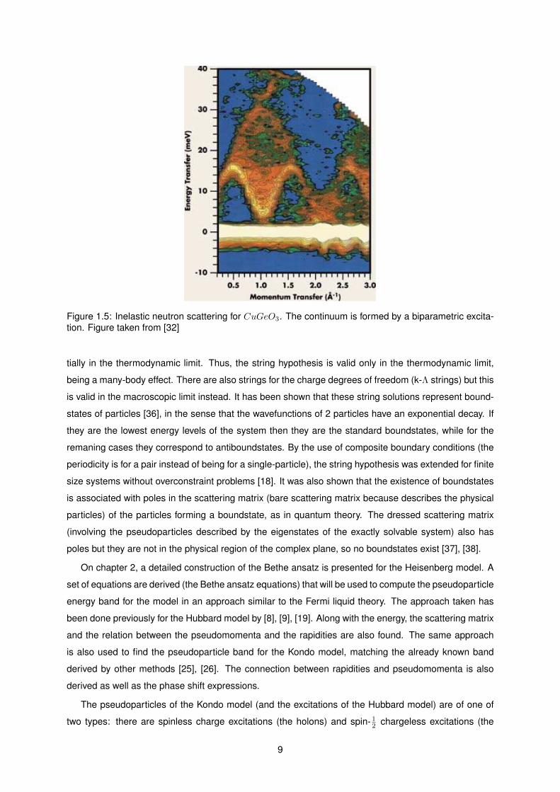
Figure 1.5: Inelastic neutron scattering for CuGeO3. The continuum is formed by a biparametric excita-tion. Figure taken from [32]
tially in the thermodynamic limit. Thus, the string hypothesis is valid only in the thermodynamic limit,
being a many-body effect. There are also strings for the charge degrees of freedom (k-Λ strings) but this
is valid in the macroscopic limit instead. It has been shown that these string solutions represent bound-
states of particles [36], in the sense that the wavefunctions of 2 particles have an exponential decay. If
they are the lowest energy levels of the system then they are the standard boundstates, while for the
remaning cases they correspond to antiboundstates. By the use of composite boundary conditions (the
periodicity is for a pair instead of being for a single-particle), the string hypothesis was extended for finite
size systems without overconstraint problems [18]. It was also shown that the existence of boundstates
is associated with poles in the scattering matrix (bare scattering matrix because describes the physical
particles) of the particles forming a boundstate, as in quantum theory. The dressed scattering matrix
(involving the pseudoparticles described by the eigenstates of the exactly solvable system) also has
poles but they are not in the physical region of the complex plane, so no boundstates exist [37], [38].
On chapter 2, a detailed construction of the Bethe ansatz is presented for the Heisenberg model. A
set of equations are derived (the Bethe ansatz equations) that will be used to compute the pseudoparticle
energy band for the model in an approach similar to the Fermi liquid theory. The approach taken has
been done previously for the Hubbard model by [8], [9], [19]. Along with the energy, the scattering matrix
and the relation between the pseudomomenta and the rapidities are also found. The same approach
is also used to find the pseudoparticle band for the Kondo model, matching the already known band
derived by other methods [25], [26]. The connection between rapidities and pseudomomenta is also
derived as well as the phase shift expressions.
The pseudoparticles of the Kondo model (and the excitations of the Hubbard model) are of one of
two types: there are spinless charge excitations (the holons) and spin- 12 chargeless excitations (the
9

spinons). It should be noted that in the literature the terms holons and spinons appear to describe
entities different from those defined here. These pseudoparticles decouple in the Kondo model (and in
the low energy regime of the Hubbard model [3]) and also enhance the spin-charge fractionalization.
The physical electrons correspond to a coherent superposition of both types of these pseudoparticles
[3].
Despite the fractionalization, not always these pseudoparticles decouple completely and may interact
with each other. As the pseudoparticles of the Bethe ansatz are known to not form boundstates between
them (and strings will not be considered), it will be analyzed the boundstates of pseudoparticles related
separately with these degrees of freedom. Instead of dealing directly with the Bethe ansatz excitations,
the work will be directed towards the binding of quasicharges and quasispins. The quasicharges and
quasispins are pseudoparticles introduced by the Ostlund-Granath transformation mentioned above.
The quasicharges are pseudoparticles living in empty or doubly occupied sites while the quasispins are
excitations living in sites with one spin down and they may be related to spinons and holons. The use
of this transformation allows the use of quantum field theory techniques to provide a Bethe-Salpeter
equation to study the binding between these pseudoparticles. The intent of this is to see if the operators
of the Ostlund-Granath representation have a similar structure to the pseudoparticles obtained from
Bethe ansatz of the Hubbard model. It has been proposed that the holons and spinons (as defined
here) are related to the Ostlund-Granath operators but for the the rotated electrons [39]. These rotated
electrons are obtained from the original electrons by an unitary transformation such that the double
occupancy is a good quantum number and the transformation reduces to the identity in the limit U →∞.
A way of finding if the pseudoparticles become bound is through the use of the Bethe-Salpeter
equation. The Bethe Salpeter equation is any equation of the form
M(p, p′;P ) = ν(p, p′;P ) +
∫ddkν(p, p′;P )G(k, P, )M(k, p′;P ) (1.16)
where M is the scattering amplitude, ν is the interaction kernel and G(k, P, ) is a two-body propagator.
Considering the interaction of the excitations, it can be seen that the scattering matrix connecting the
initial states and the final states has a pole when a bound state is formed [4]. The pole condition can
be illustrated by considering the case of a particle moving in one dimension in the presence of a square
potential well. Outside the region of the potential the states are plane waves ψl = Aeikx + Be−ikx and
ψr = Ceikx + De−ikx representing the incoming and outgoing waves in the region to the left and to
the right of the potential respectively. The S-matrix connecting the incoming and outgoing amplitudes is
given by: BC
= S
AD
(1.17)
By solving the stationary Schrodinger equation we obtain for the scattering matrix S connecting the
states
10

S = u(k, k′)
2(k′2 − k2) sin(2k′a) ϑ(k, k′)
4kk′ 2(k′2 − k2) sin(2k′a)
(1.18)
where
ϑ(k, k′) =1
4kk′
(4 sin2(2k′a)(k′2 − k2)2 − e2i(k+k′)a
((k′ − k)2e2ik′a + (k′ + k)2e−2ik′a
)·
·((k′ − k)2e2ika − (k′ + k)2e−2ika
))(1.19)
u(k, k′) =ie−2ik′a
(k − k′)2e2ika − (k + k′)2e−2ika(1.20)
and k′ =√
2m(E − V ). This matrix has a pole when(k−k′k+k′
)2
= e−4ika. For this to happen, the
momentum k must be a pure imaginary which corresponds to E < 0. Thus the poles show the conditions
to form a boundstate. The analysis of the poles of the scattering matrix associated with excitations
related to these excitations can be used to find the boundstates and their energies.
The Bethe Salpeter equation was already used to study the binding of these pseudoparticles for the
unidimensional anisotropic t-J model. Its Hamiltonian is
H =∑
<i,j>,σ
[− tc†i,σcj,σ +
Jz2
(Szi S
zj + αS+
i S−j −
ninj4
)](1.21)
The use of the Bethe-Salpeter equation, along with density matrix renormalization group methods and
exact diagonalization were done by [5] to study the binding of the spinon and holon. It was found that the
anisotropy parameter α = J⊥Jz
strongly controls the binding and alluded for the possibility that the change
in the spinon energy spectrum is the main responsible for such binding. This is a consequence of the
quasirelativistic behaviour of the spinon spectrum, causing the much heavier holon to have a secondary
role in the pairing. They also proposed a spinon-holon interaction in the form Vq,q′ = −√ωqωq′ .
On chapter 4, the boundstates found and their binding energy (along with its dependence on the
parameters involved) are presented for every combination of two excitations. The effect of considering
the self-energy in the interactions is also studied.
In chapter 5, it is analysed the transition to the bidimensionality of the Hubbard chain by introducing a
chain coupling in the form of a hopping. This hopping has a relative amplitude α that can be tuned to go
from the uncoupled chains to the isotropic square lattice. The corresponding boundstates and binding
energies are found and its evolution as functions of α is monitored.
11

12
Chapter 2
Bethe ansatz excitations
2.1 The Bethe-ansatz for the Heisenberg model
Unidimensional systems provide an example of integrable systems due to the almost centenary Bethe’s
educated guess [17]. The first N particle exactly solvable system was the isotropic Heisenberg chain with
first neighbour interactions, descring an unidimensional insulator with interacting spins. Its hamiltonian
is
H = J
N∑r
~Sr ~Sr+δ (2.1)
If J < 0, the goundstate is composed of N aligned spins (that can be along the z direction without
loss of generality) and the excited states can be constructed by flipping the spins of the groundstate
|GS〉. The first excited state is simply composed by a spin opposing all others and can be constructed
as
|Ω1〉 =∑n
ψnS−n |GS〉 (2.2)
and the excited state’s energy is given by
H|Ω1〉 =∑n
ψn(S−nH + [H,S−n ]
)|GS〉 = E1|Ω1〉 ⇔ E1ψn = EGSψn +
J
2(ψn+1 + ψn−1 − 2ψn) (2.3)
where was used the identity
[H,S−n ]|GS〉 =J
2(S−n+1 + S−n−1 − 2S−n )|GS〉 (2.4)
The ansatz to be made consists in asserting that the coefficients ψn are of the form ψn = Aeikn.
This leads to a single spin excitation energy of E = EGS +J(cos k− 1). An excited state of two spin flips
can be formed in the same way by
|Ω2〉 =∑n1,n2
ψn1,n2S−n1S−n2|GS〉 (2.5)
13

and with its energy
H|Ω2〉 =∑n1,n2
ψn1,n2
(S−n1
H + [H,S−n1])S−n2|GS〉 = E2|Ω2〉 ⇔
⇔ E2ψn1,n2=EGSψn1,n2
+J
2(ψn1,n2+1 + ψn1,n2−1 + ψn1+1,n2 + ψn1−1,n2 − 4ψn1,n2) (2.6)
obtained by the same procedure and considering non-neighbouring spins. Defining the coefficients as if
the system’s excitations were free (i.e. the ψn are taken to be combinations of plane waves)
ψ(n1 < n2) = Aeik1n1+ik2n2 +Beik1n2+ik2n1
ψ(n1 > n2) = Aeik1n2+ik2n1 +Beik1n1+ik2n2
(2.7)
will lead to an energy E2 = EGS + J(cos k1 + cos k2 − 2). As S = 12 , no consecutive spin down flips can
occur in the same site, for which the coefficient ψnj ,nj can be taken to be zero. When the spins are on
neighbouring sites (n2 = n1 + 1), the block formed has a different energy and the corresponding energy
is
E2ψn1,n1+1 = EGSψn1,n1+1 +J
2(ψn1−1,n1+1 + ψn1,n1+2 − 2ψn1,n1+1) (2.8)
and with the ansatz made, the relation between the coefficients is found to be
A
B=λ1 − λ2 − 2i
λ1 − λ2 + 2i= e2iφ(λ1−λ2) (2.9)
using the auxiliary variable λj = cotkj2 . This quantity is called rapidity and is used throughout the Bethe-
ansatz literature [3]. The factor S = e2iφ(λ1−λ2) relates the wavefunction’s amplitudes in different regions
(n1 < n2 and n1 > n2) and so corresponds to the scattering matrix S (as A = SB). Due to the lack of
inner degrees of freedom S is just composed of a phase shift φ given by
cotφ(λ1 − λ2) =1
2(λ1 − λ2) (2.10)
and from its form the scattering matrices always commute (hence obeying the Yang-Baxter relations).
Attributing a factor of eiφ(λ1−λ2) to A and e−iφ(λ1−λ2) to B, it is simple to see that any M flipped down
state can be written in the form
|ΩM 〉 =∑nj
(ψnj
M∏j=1
S−nj
)|GS〉 (2.11)
with the coefficients ψnj being
ψ(nj) =∑P
ei∑Mj kjnj+i
∑Mi>j sgn(n1−nj)φ(ki,kj) (2.12)
and with the energy
E = EGS + J
M∑j=1
(cos kj − 1) (2.13)
14

Imposing periodic conditions to the system, if an excitation j scatters with all the other particles of the
system and returns to its place, the final state must be the same apart a phase factor of eikjN , being
L = Na the system’s size and a the lattice size already englobed in the momenta. Then, the action of
the operator Tj representing the described scattering
Tj = Sj,j+1...Sj,NSj,1...Sj,j−1 (2.14)
is simply to affix the eikjN factor to the state and with the definition of the scattering matrix and taking
the logarithms one easily arrives at
kjL = 2πIj + 2
M∑l 6=j
φ(λj − λl) (2.15)
where the numbers Ij arise from the complex logarithm. Noting that the scattering matrix is simply an
exponential of phase shifts, from its definition and using
e−ikj =cot
kj2 − i
cotkj2 + i
=λj − iλj + i
(2.16)
the exponential form of eq. 2.15 leads to the Bethe ansatz equations for the Heisenberg chain
(λj + i
λj − i
)N=
M∏l 6=j
λj − λl + 2i
λj − λl − 2i(2.17)
Noting that the value of the fractions lie in the unit circle on C, one can take once again the logarithm of
both sides of eq. 2.17 and using the trigonometric identity tan(φ± π2 ) = −cot(φ) results in the logarithmic
Bethe ansatz equations:
2N arctan(λj)
= 2πIj + 2
M∑l=1
arctan
(λj − λl
2
)(2.18)
The set of M numbers can be used to determine the physical properties of the model and thus play
a role of quantum numbers [16] (because the number of spin-up and spin-down electrons are good
quantum numbers) and are integers (half-integers) if N-M-1 is even (odd). As arctan function is bounded
and to uniquely define the system’s state , the quantum numbers Ij must be on the interval
Ij ∈
[− N −M − 1
2,N −M − 1
2
](2.19)
A pseudomomentum can also be defined with these quantum numbers as
qj =2π
NIj (2.20)
with q ∈ [−π, π] in the thermodynamic limit. All the physical quantities can be described in terms of these
15

pseudomomenta or in terms of the rapidities. The energy term is
E − EGS = J
M∑j=1
(cos kj − 1) = −2J
M∑j=1
1
4λ2j + 1
(2.21)
and the magnetization can be given by
〈Sz〉 =N
2−M =
N
2−∫
dq
2πN(q) (2.22)
with N(q) being the extension to the continuum limit of the counting function.
In the macroscopic limit, the continuum Bethe-ansatz equation is
q = 2 arctan(λ(q)
)− 1
π
∫dq′N(q′) arctan
(λ(q)− λ(q′)
2
)(2.23)
and in this limit, the energy is
E = −JNπ
∫dq N(q)
1
1 + 4λ2(q)(2.24)
where the function N(q) : [−π;π[→ R is an extension to the interval [−π;π] of the function counting the
existence (=1) or inexistence (=0) of a given pseudomomentum on that interval. These pseudoparticles’
spin is also known to be 12 [20]. The spin can be found by the observation that the excitations of the sys-
tem always occur in pairs (when the particle number is conserved) and that the change in magnetization
for such an excitation is 1 [3].
2.2 Bethe ansatz excitations for the Heisenberg model
Eq. 2.23 is enough to fully describe the macroscopic behaviour of the model, but its hermetic structure
hinders the extraction of direct information about its properties. However the low-lying excitations can
be retrieved by expanding the energy near its groundstate value. The same expansion can be done for
the rapidity and the pseudomomentum distribution (N(q)) functions close to their groundstate values as
well. Hence, E = E0 +E1 +E2 + ..., λ(q) = λ0(q)+λ1(q)+λ2(q)+ ... and N(q) = N0(q)+δ(q). By doing
such an expansion, one is forcing the treatment of N0(q) as the groundstate distribution and δ(q) as an
excitation of a pseudoparticle from the groundstate distribution as in Fermi liquid theory. The example
given earlier for obtaining the Bethe ansatz equations was for the ferromagnetic Heisenberg chain. For
the antiferromagnetic case, the groundstate from which the excitations are created is composed by a
chain of misaligned spins, i.e. |GS〉 = |... ↑↓↑↓↑↓↑ ...〉, so M = N2 . The same construction of the Bethe
ansatz equations for the antiferromagnetic case will lead to equations identical to the ferromagnetic case.
In this case E0 is the groundstate energy and E1 is the 1st order correction
E1 =N
2π
∫dqε(q)δ(q) (2.25)
16

corresponding to the pseudoparticles’ band.
E2 =N
(2π)2
∫∫dqdq′
1
2f(q, q′)δ(q)δ(q′) (2.26)
The 2nd order correction to the energy can be seen as an interaction between two pseudoparticles
out of N0(q). Defining the zero energy as ε(±kF,↓) = 0, expanding in Taylor series the arctan function
and substituting the expansions in the expressions above and grouping the terms according to their
order gives, for the smaller order energy corrections
E0 = −|J |Nπ
∫dq N0(q)
1
1 + 4λ20(q)
(2.27)
E1 = −|J |Nπ
∫dq
[N0(q)
(− 8
λ0(q)
1 + 4λ20(q)
λ1(q)
)− δ(q) 1
1 + 4λ20(q)
](2.28)
E2 = −|J |Nπ
∫dq
[N0(q)
(− 8λ0(q)(
1 + 4λ20(q)
)2λ2(q) + 4(12λ2
0(q)− 1)(1 + 4λ2
0(q))3λ2
1(q)
)
− δ(q) 8λ0(q)(1 + 4λ2
0(q))2λ1(q)
](2.29)
while the terms for the Bethe-ansatz equation are
q = 2 arctan(2λ0(q)
)− 1
2π
∫dq′N0(q′)2 arctan
(λ0(q)− λ0(q′)
)(2.30)
0 =4λ1(q)
1 + 4λ20(q)
− 1
π
∫dq′
(N0(q′)
[λ1(q)− λ1(q′)
1 +(λ0(q)− λ0(q′)
)2]
+ δ(q′) arctan(λ0(q)− λ0(q′)
))(2.31)
These terms will determinate respectively the groundstate and first order correction to the rapidities
distribution. To obtain them, an auxiliary variable Q1 defined by
λ1(q) =dλ0(q)
dqQ1(q) (2.32)
is used. Taking the total derivative of eq. 2.30 with respect to q, one obtains
1 =dλ0(q)
dq
(4
1 + 4λ20(q)
− 1
π
∫dq′N0(q′)
1
1 + (λ0(q)− λ0(q′))2
)(2.33)
and with the use of eq. 2.32 , the substitution of this result in 2.31 will lead to
Q1(q) =1
π
∫dq′(δ(q′) arctan
(λ0(q)− λ0(q′)
)−N0(q′)Q1(q′)
dλ0(q)
dq
1
1 + (λ0(q)− λ0(q′))2
)(2.34)
17

In order to obtain meaningful results, it is convenient to write Q1 as
Q1(q) =
∫dq′ δ(q′)φ(q, q′) (2.35)
where φ(q, q′) turns out to be the phase shift of pseudoparticles with pseudomomenta q and q’. The
identification of φ with the phase shift comes from the already known phase shift for the model. Those
phase shifts were obtained by the difference between a particle’s momentum quantized on a ring and
the free particle’s momentum [3]. The insertion of this new expression in eq. 2.34 provides
φ(q, q′) =1
πarctan
(λ0(q)− λ0(q′)
)− 1
π
∫dq′′ N0(q′′)
dλ0(q′′)
dq′′1
1 + (λ0(q)− λ0(q′′))2φ(q′′, q′) (2.36)
As it is easier to solve the expression for the phase shift in terms of the rapidities, they will be used
instead. Changing the variable of integration to λ0, considering λ0(±qFS) = ±∞ in zero magnetic field
(where qFS is the Fermi pseudomomentum) and dropping the index 0 will lead to
φ(λ, λ′) =1
πarctan
(λ− λ′
)− 1
π
∫R
dλ′′1
1 + (λ− λ′′)2φ(λ′′, λ′) (2.37)
As the phase shift is simply a function of the rapidity difference, its derivative f(λ) = ∂λφ(λ − λ′)
obeys the equation
f(λ) =1
π
1
1 + λ2− 1
π
∫R
dλ′′1
1 + (λ− λ′′)2f(λ′′) (2.38)
obtained by integrating by parts. Performing the Fourier transform on both sides of the equation leads to
f(ω) =1
1 + e|ω|(2.39)
Inverting the Fourier transform, one gets
f(λ) =1
4π
(− ψ
[1
2− iλ
2
]+ ψ
[1− iλ
2
]+ ψ
[1 +
iλ
2
]− ψ
[1
2+iλ
2
])(2.40)
where ψ is the digamma function. Thus the final expression for the phase shift is
φ(λ) =i
2πlog
(Γ[1− iλ
2
]Γ[
12 + iλ
2
]Γ[1 + iλ
2
]Γ[
12 −
iλ2
]) (2.41)
by forcing φ(0) = 0.
The groundstate density distribution of the rapidities is also easily calculated via the same path.
Defining
σ(λ) =dq
dλ0(2.42)
it is easy to see that by multiplying σ on both sides of eq. 2.33, one arrives at an equation similar to the
one for the phase shifts
σ(λ) =4
1 + 4λ2− 1
π
∫dλ′
1
1 + (λ− λ′)2σ(λ′) (2.43)
18
where to maintain consistency the change of variable in the integration obliges
∫ +∞
0
dλσ(λ) = kF,↓ (2.44)
Once more, through the use of Fourier transforms and algebraic manipulations, eq. 2.43 becomes
σ(ω) = π1
cosh |ω|2(2.45)
and inverting the result,
σ(λ) = π1
cosh(πλ)(2.46)
Integrating σ and setting λ0(0) = 0, the relation between the pseudomomenta and the rapidities is
found to be
tan(q
2
)= tanh
(π2λ0(q)
)(2.47)
The pseuparticle band can now be obtained without much effort. Substituting 2.32 in the equation
for E1 and using the definition of Q1 leads to
ε(q) = −|J |2
114 + λ2
0(q)+ |J |
∫dλ′ φ(λ′, λ0(q))
λ14 + λ′2
(2.48)
Instead of substituting directly the result obtained for φ(λ) it is easier to obtain the pseudoparticle
band by defining
η(λ) =dε(q)
dλ0(q)(2.49)
and observe that through the use of eq. 2.38, one can build an analogous integral equation for η(λ) by
simply multiplying and integrating eq. 2.38 by the appropriate factors to obtain
η(λ) = −|J | λ
( 14 + λ2)2
+1
π
∫dλ′
1
1 + (λ− λ′)2η(λ′) (2.50)
Performing once again the Fourier transform will result in
η(ω) = |J |πie− 12 |ω|ω − e−|ω|η(ω)⇔ η(ω) =
|J |πiω2 cosh(ω2 )
(2.51)
Inverting the Fourier transform, the expression for the pseudoparticle band is
ε(q) = −|J |π2
1
cosh(πλ0(q))= −|J |π
2cos(q) (2.52)
The pseudoparticle energy is lower for pseudomomenta around zero so that in the groundstate all
pseudoparticles will form a Fermi sea centred around zero. The quantum numbers of the system will then
pack closely to each other around that value at the groundstate and any excitations can be described by
placing holes in the groundstate distribution or adding numbers outside the set. Hence, the excitations
of the system are simply obtained by considering a pseudoparticle with momentum and energy opposite
19

to the vacant site, analogous to particle-hole excitations.
Figure 2.1: Pseudoparticles’ band in function of the pseudomomentum. The groundstate is a compactset of pseudomomenta centred around 0. A possible excitation is the removal of a pseudomomentumfrom the set and the filling of a vacant slot like particle-hole excitations.
The energy band and the phase shifts obtained here are key pieces for calculating experimental
exponents like the spin dynamical structure factor.
2.3 Dynamical spin structure factor of the Heisenberg chain
With the obtention of the energy bands and phase shifts of the model and with the use of the appropriate
ensemble, equilibrium properties are easy to compute. However, the dynamical properties are more
difficult because they demand an evaluation of matrix elements and the knowledge of the wavefunctions
of the model. Bethe ansatz provides the exact N-particle wavefunction, but not only the expressions
obtained this way are very complicated, the relation between the Bethe ansatz quantum numbers and the
particle operators of the system is in general unknown. Nevertheless, the Heisenberg model constitutes
an exception to this, where the matrix elements are known and can be obtained by the factor method.
An operator description of the Bethe ansatz solution has been proposed, allowing an approximate
calculation of some correlation functions of the Hubbard model [10]. These include the calculation of
the spectral function [11], [23] and the charge dynamical structure factor at half-filling [12]. To obtain
the dynamical structure factor for the Heisenberg model, one can use the results known for the Hubbard
model, and note that at half-filling and in the limit U →∞, the Hubbard-model reduces to the Heisenberg
model. Additionally, the corresponding expressions for the Heisenberg model can then be obtained by
disregarding the contributions of the charge degrees of freedom to the phase shifts (of the Hubbard
20

model). The spin dynamical structure factor is given by the groundstate correlation functions
Ssinglet(k, ω) =1
N
∑j,l
eikl∫ +∞
−∞dteiωt〈GS|Szj Szj+l|GS〉 (2.53)
or
Striplet(k, ω) =1
N
∑j,l
eikl∫ +∞
−∞dteiωt〈GS|S+
j S−j+l|GS〉 (2.54)
involving spin singlet or spin triplet excitations. At zero magnetic field these excitations are degener-
ate and the system retains its SU(2) invariance. The key step to evaluate this correlation function is
to observe which allowed processes couple the groundstate with the excited states and assess their
contribution. The simplest case involves the creation of two spinons for the spin triplet excitation case,
and it turns out to be the most important. The remaining allowed processes, involving excitations of a
larger number of spinons or strings with complex rapidities (the case of the singlet), have very small
contributions to the spectral weight so it is enough to consider the dominant term of two spinons.
The two spinons are holes of the energy band of the spin pseudoparticles both in the Hubbard model
and in the Heisenberg model. Labeling the holes’ pseudomomenta as q and q′, the energy of this excited
state is given by
ω(k) = −εs(q)− εs(q′) (2.55)
where k is the momentum of the excitation given by
k = π − q − q′ (2.56)
The momentum π arises because the excitation induces an overall π-shift due to the change of the
quantum numbers from half-integers to integers. At zero magnetic field, both pseudomenta lie in the
interval [−π/2, π/2]. Recall that the spectrum is the same for both spin triplet and spin singlet excitations.
Due to the biparametric excitation (since there is a contribution of two spinons), the excitation spec-
trum is a continuum. The lowest energy line corresponds to keeping one hole at a Fermi point while
the other hole sweeps the whole energy band. Below this line there is no spectral weight and above it,
the spectral weight decreases algebraically with an exponent that has been determined before for the
Hubbard model. This dependence can be written as
Ss(k, ω) ∼ (ω − ωs(q))−1+ξ0 (2.57)
By analogy with what has been done before for the Hubbard model, the exponent of this lower line is
given by
ξ0 = 2∆1s + 2∆−1
s (2.58)
21

where
2∆1s =
[1
2ξ1 + Φ(q0
FS , q)
]2
2∆−1s =
[1
2ξ1 + Φ(−q0
FS , q)
]2
(2.59)
and where Φ is the phase shift, q is the spinon’s pseudomomentum,
ξ1 = 1 + Φ(∞,∞)− Φ(∞,−∞) (2.60)
and q0FS = kF,↓ = kF,↑. The energy line where the power law is calculated is given by
ω(k) = −εs(π − k) (2.61)
where εs(q) is spinon energy band calculated above. Using Eqs. (62,66,67,68) and Eq. (B1) of [9] and
comparing with Eq. (5.3) of [13], the phase shift values at λ = ±∞ are
Φ(∞,−∞) =
√2
4(2.62)
and
Φ(∞,∞) =3√
2
4− 1 (2.63)
Therefore
ξ1 =1√2
(2.64)
ξ0 can also be calculated. Its value is
ξ0 =
[1
2√
2+ Φ(∞, λ0(q))
]2
+
[1
2√
2+ Φ(−∞, λ0(q))
]2
+
=
[1
2√
2+
1
2√
2
]2
+
[1
2√
2− 1
2√
2
]2
=1
2(2.65)
Therefore the exponent is given by
− 1 + ξ0 = −1
2(2.66)
This result agrees with the value obtained by other methods such as the limit U → ∞ of the half-
filling Hubbard model and the form factor method. It is however easier to obtain the exponent using the
pseudofermion dynamical theory developped for the Hubbard model and provides a nontrivial application
of the results obtained in this section.
22

2.4 The Kondo model
Another model with an exact solution via the Bethe ansatz is the Kondo model. The same construction
developed for the Heisenberg model can also be made for the this model as well. The Kondo model
describes an ideal electron gas interacting with a magnetic impurity in the system. Its Hamiltonian
corresponds to
H =∑k,σ
εkc†k,σck,σ + Jc†r=0,a ~σa,b cr=0,b · ~σ0 (2.67)
with ~σ0 being the impurity spin and J the coupling of the conduction band to the impurity. Further it is
assumed that only the s-wave modes couple with the impurity. Considering only the s-wave scattering,
the tridimensional system can be reduced to an unidimensional one, along the directions of the incoming
and outgoing electron and centred in the impurity. The inclusion of higher angular momentum modes
leads to the Multi-channel Kondo model and will not be discussed here. Linearizing the energy band
around the Fermi level will result in
ε(k) = ε(kF ) + vF k (2.68)
where in the following calculations vF will be taken to be 1. An electron-impurity interaction term
J ′∑σ c†r=0,σcr=0,σ can be also introduced without breaking the integrability or altering significatively
the equations. Considering a single-electron wavefunction in the form
ψ(xj) = eikxj [Aaja0θ(−xj) +Baja0θ(xj)] (2.69)
and evaluating the Schrodinger equation at xj = 0, the scattering matrix (between an electron and the
impurity) relating the Baja0 amplitude to the Aaja0 amplitude can be written as
Sj0 = e−iφIj0 − icP j0
1− ic(2.70)
where I and P are the identity and permutation operators respectively, and
c =8J
4− 3J2 − 2JJ ′ + (J ′)2(2.71)
To ensure that the Yang-Baxter equations are obeyed, the scattering matrix between electrons must take
the form Sij = P ij . Imposing periodic boundary conditions for the scattering of an electron with all the
others and the impurity, the problem turns to the diagonalization of the operator T defined by
T = P jj−1...P j1P jN ...Sj0...P jj+1 (2.72)
This will lead to the Bethe-ansatz equations for the Kondo model with a linearized band [3]
eikjL =
M∏γ=1
λγ − 1 + ic2
λγ − 1− ic2
(2.73)
23

−∏δ 6=γ
λδ − λγ + ic
λδ − λγ − ic=
(λγ − 1− ic
2
λγ − 1 + ic2
)Ne(λγ − ic2
λγ + ic2
)(2.74)
where the indexes j, γ run over all positive integers until reaching respectively the number of electrons
in the system (Ne) and the number of spin-downs M, while L is the lenght of the chain. Once again the
value of the fractions lie in the unit circle on C, so the trigonometric identity tan(φ ± π2 ) = cotφ is used
again. The logarithm of both equations can be obtained and reads
kj =2π
Lnj −
2
L
M∑γ=1
(arctan
(2λγ − 2
c
)+π
2
)(2.75)
2π
LJγ −
2
L
M∑δ
arctan
(λδ − λγ
c
)= 2D arctan
(2λγ − 2
c
)+
2
Larctan
(2λγc
)(2.76)
where nj , Jγ are the integers that arose from the logarithms and D = NeL . As before, this quantum
numbers correspond to integers/half-integers whether M is even/odd (in the case of nj) and whether
N+M+1 is even/odd (in the case of Jγ) and can also be used to define the pseudomomenta
Qj =2π
Lnj qγ =
2π
LJγ (2.77)
The energy of the linearized band can be written in terms of the rapidities and pseudomomenta as
E =
Ne∑j=1
kj =
Ne∑j=1
Qj −M∑γ=1
qγ −2
L
M∑γ=1
arctan
(2λγc
)
=
Ne∑j=1
Qj − 2D
M∑γ=1
(arctan
(2λγ − 2
c
)+π
2
)(2.78)
From the first expression to the energy, it can be seen that the first term is the contribution of the
charge pseudomomenta Qj to the energy, the second is the spin pseudomomenta qj contribution and
the last term is the energy of the magnetic coupling to the impurity. The separate contribution to the
energy enhances the spin-charge separation. It also reveals the charge contribution is simply the energy
of a free electron gas, as expected from the physics of the Kondo model. By the same arguments used
before, as the excitations of the charge part do not change the magnetization of the system, the charge
excitations have spin 0. As the charge part is trivial, the attention will fall only on the spin part. In the
continuum limit, the equations become
q = 2D arctan
(2λ(q)− 2
c
)+
2
Larctan
(2λ(q)
c
)+
1
π
∫dq′ N(q′) arctan
(λ(q)− λ(q′)
c
)(2.79)
E =Ne2π
∫dq(− 2 arctan
(2λ(q)− 2
c
)− π
)(2.80)
It should be noted that apart from constants, the Bethe ansatz equation for the Kondo model is similar
to the one for the Heisenberg with an impurity term of 2L arctan
( 2λ(q)c
). This term vanishes in the macro-
scopic limit (as expected since a single impurity contribution cannot shield itself) and the comparison
24
with real systems must take into account instead an impurity density (which would lead to the substitu-
tion 1L → n, with n being the impurity density). This impurity density must be low enough so no additional
interactions between the impurities appear. The Fermi liquid approach taken for the Heisenberg can now
be used for the Kondo model. Expanding the energy, the rapidity and the pseudomomentum distribution
function near their value and distribution functions of the groundstate, such that E = E0 +E1 +E2 + ...,
λ(q) = λ0(q) + λ1(q) + λ2(q) + ... and N(q) = N0(q) + δ(q) as before, and substituting the expansions in
the expressions above and grouping the terms according to their order gives for the energy terms
E0 =Ne2π
∫dq N0(q)
[(− 2 arctan
(2λ0(q)− 2
c
)− π
)](2.81)
E1 =Ne2π
∫dq
[N0(q)
(4
c
λ1(q)
1 +(
2λ0(q)−2c
)2
)− δ(q)(2 arctan
(2λ0(q)− 2
c
)+ π)
](2.82)
E2 =Ne2π
∫dq
[N0(q)
(− 4
c
λ22(q)
1 +(
(2λ0(q)−2)2
c
) +16
c3λ0(q)− 1(
1 + 4c2 (λ0 − 1)2
)2λ21(q)
)
− 4
cδ(q)
λ1(q)
1 +(
2λ0(q)−2c
)2
](2.83)
and for the Bethe-ansatz equation terms
q = 2D arctan(2
c(λ0(q)− 1)) +
2
Larctan(
2
cλ0(q))− 1
π
∫dq′N0(q′) arctan(
1
cλ0(q)− λ0(q′)) (2.84)
0 =4D
c
λ1(q)
1 + ( 2c (λ0(q)− 1))2
+4
Lc
λ1(q)
1 + ( 2cλ0(q))2
− 1
π
∫dq
[N0(q)
(− λ1(q)− λ1(q′)
c
1
1 +(
(λ0(q)−λ0(q′))2
c
))+ δ(q′) arctanλ0(q)− λ0(q′)
c
](2.85)
Defining the same auxiliary variable Q1 as in eq. 2.32 and taking the derivative of eq. 2.84 , the zero
order equation becomes
1 =dλ0(q)
dq
(4D
c
1
1 + ( 2c (λ0(q)− 1))2
+4
Lc
1
1 + ( 2cλ0(q))2
− 1
πc
∫dq′N0(q′)
1
1 + ( 1c (λ0(q)− λ0(q′)))2
)(2.86)
and its substitution into 2.85
Q1(q) =1
π
∫dq′ δ(q′) arctan
(λ0(q)− λ0(q′)
c
)− 1
π
∫dq′ N0(q′)
Q1(q′)
c
dλ0(q)
dq
1
1 + (λ0(q)−λ0(q′))c )2
(2.87)
Recalling that Q1 can be related to the phase shift by eq.2.35, the equation for the phase shifts can
25

be found to be
φ(q, q′) =1
πarctan
(λ0(q)− λ0(q′)
c
)− 1
π
∫dq′′ N0(q′′)
φ(q, q′)
c
dλ0(q′′)
dq′′1
1 + (λ0(q)−λ0(q′′))c )2
(2.88)
and changing the variable of integration to λ will provide
φ(λ, λ′) =1
πarctan
(λ− λ′
c
)− 1
πc
∫dλ′′
1
1 +(λ−λ′′c
)2φ(λ′′, λ′) (2.89)
Apart from the c factor the phase shift found is identical to the one for the Heisenberg model. This
means that the phase shift between the spinons is not changed by the impurity. Defining the f function
as previously (f(λ) = ∂λφ(λ− λ′) ), the phase shift integral equation will lead to
f(λ) =1
πc
1
1 + (λc )2− 1
πc
∫dλ′
1
1 + ( 1c (λ− λ′))2
f(λ′) (2.90)
and performing the Fourier tranform,
f(ω) =1
1 + ec|ω|(2.91)
The inverse Fourier transform holds
f(λ) =1
4πc
(− ψ
[1
2− iλ
2c
]+ ψ
[1− iλ
2c
]+ ψ
[1 +
iλ
2c
]− ψ
[1
2+iλ
2c
])(2.92)
with ψ being the digamma function. The integration provides the phase shift
φ(λ) =i
2πlog
(Γ[1− iλ
2c
]Γ[1 + iλ
2c
]Γ[
12 + iλ
2c
]Γ[
12 −
iλ2c
]) (2.93)
Via the same procedures, the relation between the pseudomomentum and the rapidities is obtained
defining the density
σ(λ) =dq
dλ0(2.94)
and resorting to eq. 2.86 one can also obtain an integral equation for σ(λ)
σ(λ) =4D
c
1
1 + ( 2c (λ− 1))2
+4
Lc
1
1 + ( 2cλ)2
− 1
πc
∫dλ′
1
1 + ( 1c (λ− λ′))2
σ(λ′) (2.95)
using that ∫dλ′ σ(λ) = kF,↓ (2.96)
Solving the eq. 2.95 through Fourier transforms as before will result in
σ(ω) = 2π
(Deiω +
1
L
)1
2 cosh c|ω|2
(2.97)
26

and inverting the Fourier transform
σ(λ) =π
Lc
1
cosh πλc
+πD
c
1
cosh πc (λ− 1)
(2.98)
Through the definition of σ, the relation between the pseudomomentum and the rapidity is
q =2
Larctan tanh
(π
2cλ0
)+ 2D arctan tanh
(π
2c(λ0 − 1)
)+ 2D arctan tanh
(π
2c
)(2.99)
It should be noted that the impurity introduces an extra term in the relation between the pseudomo-
mentum and the rapidity due to the scattering with the impurity. The only thing left is the pseudoparticle
band. By substituting the Q1 definitions in the first order correction to the energy, one obtains the band
equation
ε(q) = D
[− 2 arctan
(2λ0(q)− 2
c
)− π
]− 4D
c
∫dλ′
1
1 +(
2λ′−2c
)2φ(λ′, λ0(q)) (2.100)
Defining the η function as
η(λ) =dε(q)
dλ0(q)(2.101)
the equation for the band can be written as
η(λ) = −4D
c
1
1 +(
2c (λ− 1)
)2 − 1
πc
∫dλ′
1
1 +(
1c (λ− λ′)
)2 η(λ′) (2.102)
The Fourier transform of the equation provides the solution
η(ω) = −2πDeiω
2 cosh(cω2
) (2.103)
and the inverse Fourier transform
η(λ) = −πDc
1
cosh(π λ−1
c
) (2.104)
can be used to obtain the pseudoparticle band
ε(q) = −2D arctan eπc (λ0(q)−1) (2.105)
Once again, the system’s excitations are created by placing holes and filling vacant slots outside the
compact groundstate distribution.
27

Figure 2.2: Pseudoparticles’ band in function of the rapidities for D=1 and c = 14 .
28

Chapter 3
The unidimensional Hubbard model
3.1 The Hubbard model and its extensions
The Hubbard model defined in eq. 1.14 can be written as particle-hole symmetric with a rescaled
Hamiltonian as
H = −∑r,σ
(c†r,σcr+δ,σ + c†r+δ,σcr,σ
)+u
2
∑r
(nr − 1)2 (3.1)
where u = Ut , t=1 and no summation on δ occurs because bonds are only counted once and r+δ stands
only for the neighbouring site to the right of r. The term (nr − 1)2 comes from nr,↓nr,↑ = 12 (nr − 1 +
(nr − 1)2) and one can choose an appropriate chemical potential to sweep away the remaining terms.
Due to the separation of the degrees of freedom in unidimensional systems, as shown previously, it
should be possible the existence of a transformation that acts on the electronic operators and returns
new operators that exhibit the expected splitting. One possible transformation is the Zou-Anderson
transformation mentioned earlier. However this transformation needs an additional constraint to restrain
the enlargement of the Hilbert space, which turns any computation more lengthy, and in general the
constraint is not implemented exactly. Another possible transformation that overcomes this problem is
the Ostlund-Granath transformation. In this transformation, new operators are introduced such that one
type of the new creation operators only acts on singly occupied sites and the other type of creation
operator acts on sites with a spin down. These new operators, called the quasicharge cr and the
quasispin qir, are related to the electronic operators by:
cr = c†↑,r(1− n↓,r) + (−1)rc↑,rn↓,r
q+r =
(c†↑,r − (−1)rc↑,r
)c↓,r
q−r =(q+r
)†qzr = 1
2 − n↓,r
(3.2)
The quasicharges represent spinless fermions since they obey the algebra cr, c†r′ = δr,r′ and
cr, cr′ = 0 while the quasispin represent spin 12 due to [qir, q
jr′ ] = iδr,r′εijkq
kr . As it is a fraccionaliza-
tion transformation, they also disengage from each other since they commute The original electronic
29

operators can be written in terms of these new operators by
cr,↑ = c†r(12 + qzr ) + (−1)rcr(
12 − q
zr )
cr,↓ = (c†r − (−1)rcr)q+r
(3.3)
There are other operators provenient from this representation such as the quasicharge number ncr =
c†rcr and some useful relations associated such as nr = 1 − 2ncrqzr , (nr − 1)2 = ncr and sir = (1 − ncr)qir
(a) (b)
(c) (d) (e)
Figure 3.1: Quasicharge and quasispin operator actions on the states.
that can be immediately verified by applying them to the states composing the Hilbert space. There
are other operators related with the Ostlund-Granath-transformation such as the pseudospin pir = ncrqir
and fr = c†r. The pseudospin is related to a symmetry of the particle-hole Hubbard model and the total
z-component of the pseudospin is half the charge relative to half-filling. This symmetry is broken with
the introduction of a chemical potential. From the relations between the operators, one can see that the
total quasispin Q can be expressed by the sum of the total spin S and the total pseudospin P (Q=S+P).
In terms of these new operators, the Hamiltonian becomes
H = T0 + Tπ + T †π +u
2
∑r
ncr (3.4)
where,
T0 =1
2
∑r
(1 + 4~qr · ~qr+δ)(c†rcr+δ + c†r+δcr) (3.5)
Tπ =1
2
∑r
(−1)r(1− 4~qr · ~qr+δ)c†rc†r+δ (3.6)
Foretelling some difficulties to be encountered, additional terms will be added to the Hamiltonian as
an external magnetic field term Hh (aligned in the z direction without any loss of generality), a chemical
potential Hµ (that now recovers the shift made earlier and rewrites the Hubbard model as in eq. 1.14)
30

and a 1st neighbour interaction term HV .
Hh = −h∑r
szr = −h∑r
(1− ncr)qzr
Hµ =(u
2− µ
)∑r
nr =(u
2− µ
)∑r
(1− 2ncrqzr ) (3.7)
HV = V∑r
nrnr+δ = V L+ 4V∑r
ncrncr+δq
zrqzr+δ − 4V
∑r
ncrqzr
As it is desired to employ the tools of zero temperature many-body theory to analyse the excitation’s
binding, it is necessary to transform the quasicharge operators into operators that have a fermionic or
a bosonic character. Usually spin operators are represented by bilinear forms. However this leads to
interaction terms that involve six operators. It is then preferable to use a quasilinear representation.
For fermionic character we can use the Jordan-Wigner transformation. This tranformation maps the
spin 12 to a combination of fermionic operators by
q+r = d†r e
iπ∑r−1x=1 d
†xdx
q−r = e−iπ∑r−1x=1 d
†xdx dr (3.8)
qzr = d†rdr −1
2
Despite the exponential with the sum of all excitations to the left of the site the operator is acting
on, the operator pairs in the Hamiltonian simplify (q+r q−r+δ = d†rdr+δ and q−r q
+r+δ = d†r+δdr) and the
Hamiltonian in momentum space will read:
T0 =∑k
2 cos k c†kck + 2∑q,k1,k2
(cos(q + k1) + cos(q − k2)− cos k1 − cos k2
)d†q+k1−k2c
†k2ck1dq (3.9)
Tπ = 2∑q,k1,k2
(cos(q − k1)− cos(q − k2)− cos k1 + cos k2
)d†q−k1−k2+πc
†k1c†k2dq (3.10)
When Fourier transforming Tπ, one encounters the (−1)r factor which leads to a vertex that provides
an extra π momentum to the momenta of the outgoing particles and since this factor defined (mod 2π)
in momentum space, all momenta may be taken (mod 2π). The additional terms of the model become:
Hh =hL
2− h
∑k
d†kdk −h
2
∑k
c†kck + h∑q,k1,k2
d†q+k1−k2c†k2ck1dq
Hµ =(u
2− µ
)L+
(u2− µ
)∑k
c†kck + (2µ− u)∑q,k1,k2
d†q+k1−k2c†k2ck1dq (3.11)
HV = V∑
k1,k2,k3
cos(k3 − k2)c†k1+k2−k3c†k3ck2ck1 − 4V
∑q,k1,k2
d†q+k1−k2c†k2ck1dq + 2V
∑k
c†kck
A problem with using this representation is that the fermions representing the quasispins do not
form a well-defined Fermi surface because there is only a single energy level containing all the possible
momenta. To overcome this problem it shall be used instead a bosonic representation for the quasispins.
Another issue is the difficulty in generalizing the Jordan-Wigner transformation to the bidimensional
31

case. The simplest way involves the lattice partition into sublattices and makes the dynamics more
complicated.
The transformation of the quasispins to bosons is done via the Holstein-Primakoff transformation.
Since the spectrum of a spin S is similar to the S first levels of the harmonic oscillator, it is possible
to map the two systems into each other. Despite for the Hubbard model as defined here being irrel-
evant the order correspondence between the levels, it is chosen the descendant ordering. Hence the
transformation to be performed is
q+r =
√2S
√1− a†rar
2Sar ≈
√2Sar
q−r = a†r√
2S
√1− a†rar
2S≈√
2Sa†r (3.12)
qzr = S − a†rar
The approximation considered is to simply obtain a quartic Hamiltonian that is valid when the number
of excitations are small (large S regime). With this approximation, the linearization is performed and
any interactions terms of order higher than 4 are neglected. A more accurate prescription was to use
an antiferromagnetic representation since in one dimension, the groundstate is expected to be a spin
singlet. The excitations in this representation would surely be small, but at the cost of increasing the
number of diagrams to be calculated, since the antiferromagnetic representation would lead to two
types of bosons (each living on a sublattice). In the ferromagnetic representation, the Hamiltonian in
momentum space is
H =∑k
ε(k) c†kck +∑q,k1,k2
U0(q, k1, k2) a†q+k1−k2c†k2ck1aq +
∑q,k1,k2
V+(q, k1, k2) a†q−k1−k2+πc†k1c†k2aq
+∑q
h a†qaq +∑q,k1,k2
V−(q, k1, k2) a†q+k1+k2+πck1ck2aq +∑
k1,k2,k3
Ux(k1, k2, k3) c†k1+k2−k3c†k3ck2ck1
(3.13)
where the fermion band is ε(k) = 2 cos k + u2 +B and the interactions are
U0(q, k1, k2) = 2[
cos(q + k1) + cos(q − k2)−B]
(3.14)
V+(q, k1, k2) = 2(cos k2 − cos k1 + cos(k1 − q)− cos(k2 − q)) (3.15)
V−(q, k1, k2) = 2(cos k1 − cos k2 + cos(k2 + q)− cos(k1 + q)) (3.16)
Ux(k1, k2, k3) = V cos(k3 − k2) (3.17)
where B = h2 + µ − u
2 − 2V is a useful parameter that encompasses all the physical parameters of
the system and spans all R. When B = 0 it is as if all those additional terms are not inserted in the
Hamiltonian and one reencounters the physics of the particle-hole Hubbard model (at half-filling with no
magnetic field nor 1st neighbour interactions); B 6= 0 may be used to probe regimes of intense electronic
repulsion or coupling with the magnetic field. From the quasicharge’s and quasispin’s energy bands,
32

one can write directly the propagators associated with each excitation as
Quasicharge (fermionic) G0(k, ω) =ℵ(|k| − pcF )
ω − (2 cos k + u2 +B) + iη
+ℵ(pcF − |k|)
ω − (2 cos k + u2 +B)− iη
(3.18)
Quasispin (bosonic) D0(k, ω) =1
ω − h+ iη(3.19)
and represented in Figure 3.2.
Figure 3.2: Diagrammatic representation of the fermionic (G0) and bosonic (D0) propagators.
Due to the band’s dependence with k, the functions ℵ(|q| − pcF ) = Θ(pcF − |q|) and ℵ(pcF − |q|) =
1−Θ(pcF − |q|) were used (note the concave band in Figure 3.3).
Figure 3.3: Quasicharge band with the zero energy at its bottom.
The associated vertices are directly obtained from the 4 quartic terms and whose respective intensity
corresponds to eqs. 3.14 to 3.17.
Since the π-momentum vertexes (in orange in Figure 3.4) can only appear in pairs for situations
conserving the number of interacting particles, an additional antissimetrization of all possible links of the
fermionic lines conected to the vertexes must be performed. Since the vertex term is antissimetric in the
fermion momenta, it is sufficient to choose just one possibility and multiply the result by a factor of 2. A
more thorough but concise explanation of the diagrammatic rules can be found in appendix A.
33

Figure 3.4: Vertices.
3.2 The Bethe-Salpeter equation
As previously analyzed, an indicator of the occurrence of boundstates is the presence of poles in the
scattering matrix. In standard perturbation theory, one typically calculates a few low order scattering
amplitudes that provide the major contribution in the physical processes. As they usually do not diverge
(neither a finite sum of them will), no poles will ever be found in this perturbation scheme. If a boundstate
does exist, then it would appear in the exact scattering matrix of the problem, but since the sum of all
the possible diagrams is unpractical, one simply selects a class of diagrams that might dominate the
physics involved and perform their infinite sum. A particularly simple class of diagrams that can be
easily summed due to its repetitive pattern is the ladder diagram’s class. If the coupling constants are
small and if the scattering occurs at low energies, the ladder diagrams prevail over the others and their
selection can perfectly describe the boundstates’ nature [4]. The ladder diagrams consist solely of a pair
of propagators whose momenta and energies are altered by an interaction U and the scattering matrix
34

for the sum of the whole class is
M(p, P − p, p′, P − p′) =M1(p, P, p′) +
∫dd+1qG0(p)G0(P − p)U(p, P, k)M1(k, P, p′)
+
∫dd+1kG0(p)G0(P − p)U(p, P, k)
∫dd+1qG0(k)G0(P − k)U(k, P, q)M1(q, P, p′) + ... (3.20)
that has the diagrammatic correspondence in Figure 3.5 and where d stands for the spatial dimension.
Figure 3.5: Ladder diagram sum.
FromM1(p, P, p′) = G0(p)G0(P − p)U(p, P, p′)G0(p′)G0(P − p′), the infinite sum can be recognized
to be the Born series of
M(p, P −p, p′, P −p′) =M1(p, P, p′) +
∫dd+1kG0(p)G0(P −p)U(p, P, k)M(k, P −k, p′, P −p′) (3.21)
Figure 3.6: Integral equation for the scattering matrix.
Instead of dealing directly with the scattering matrix, one can define an effective interaction (defined
by the vertex function Γ(p, P − p; p′, P − p′) represented by the cerulean box) that comprises all the
intermediate states and interactions considered. The scattering matrix poles will be the exact same
poles appearing in the Γ function. It is now easy to note that each term of the sum in eq. 3.20 can be
grouped in terms of products of G0’s and U such that each nth order term is composed by a product of
2n Green’s functions and n interaction’s wavy lines connecting them. This allows to rewrite eq. 3.20 for
Γ as
Γ(p, P − p; p′, P − p′) = U(p, p′) +
∫dd+1kU(p, k)G0(k)G0(P − k)U(k, p′)+
+
(∫dd+1kU(p, k)G0(k)G0(P − k)
)∫dd+1qU(k, q)G0(q)G0(P − q)U(q, p′) + ... =
= U(p, p′) + U(p, P, k)U(k, p′) + U(p, P, k)U(k, P, q)U(q, p′) + ... (3.22)
with: U(k, P, q) =
∫dd+1q U(k, P, q)G(q, ω)G(P − q,Ω− ω) (3.23)
and noting that the infinite sum is nothing more than the geometrical series whose representation is
patent in Figure 3.7, a condition for a pole emerges.
35

Figure 3.7: Each nth order term is a nth power of a basic repeating pattern. The sum of the infinite termscan be evaluated as presented at the right.
Due to the geometrical series’ nature of the sum, for Γ to diverge, U must have an eigenvalue 1. This
is more clear if one substitutes the integrals above by sums in a finite set of values in momentum space
such that the kernel is a matrix and the n integrations of the nth order term are simply the product of the
n kernels. Diagonalizing them, and summing all terms, would produce a diagonal matrix between the
two eigenvector matrices whose elements would present the form 11−λj , where λj are the eigenvalues.
Even if the result above does not converge, the solution may still exist and can be taken as an analytical
prolongation from one region, where the converge does not occur, to another where it does. So the
divergence occurs when U has an eigenvalue of 1 and the corresponding condition for the existence of
a pole inM is
Γ(k, P − k, k′, P − k′) = U(k, P, q)Γ(q, P − q, k′, P − k′) (3.24)
This establishes a procedure to find the associated Bethe-Salpeter equation for any excitations in-
teracting via an arbitrary potential. If U is a building block whose repetition generates an infinite ladder
sum, then eq. 3.24 is the Bethe-Salpeter equation for the effective interaction Γ that alllows a solution.
Performing the integration in ω, only the terms with the poles on opposite sites of the complex plane will
contribute making the coupling occur only between excitations both above or both below the Fermi sea,
resulting in
G(q) =N(q, P )
Ω− ε1(q)− ε2(P − q)(3.25)
where N(q, P ) = Θ(ε(q)−EF )Θ(ε(P − q)−EF )−Θ(EF − ε(q))Θ(EF − ε(q)). Labeling GΓ as the pair’s
wavefunction ψ, the equation becomes
ψ(k) =1
Ω− ε1(k)− ε2(P − k)
∫dq
2πVeff (k, q)ψ(q) (3.26)
where the potential and N were agglutinated into an effective potential Veff = N(q, P )V (k, q) by conve-
nience. The identification of ψ with the wave function of the pair comes from the analogy of this equation
with the equation obtained from scattering theory for the pair after the interaction with a potential. Writ-
ting the Schrodinger equation for two particles interacting via a potential V (r) as
(E −H0(r)
)ψ(r) = V (r)ψ(r) (3.27)
where ~r = ~r1− ~r2, and using the Green’s function technique, the free particle Green’s function is obtained
36

by (E −H0(r)
)G0(r, r0) = δ(r − r0) (3.28)
whose Fourier transform assuming retarded boundary conditions (i.e. G0(t′, t) is only non-null for t > t′)
is
G0(k) =1
E −H0(k) + iη(3.29)
With this in mind, one can obtain an integral equation for the total solution ψ in the form of
ψ(r) = φ(r) +
∫G0(r, r0)V (r0)ψ(r0)dr0 (3.30)
The homogeneous solution φ(r) represents the wave function unaffected by the potential represent-
ing the free particles. The absence of this term implies that the particles cannot be free and hence must
be bound. Without the free particles’ term, eq. 3.30 in momentum space is
ψ(k) =1
E −H0(k)
∫dq
2πV (k, q)ψ(q) (3.31)
Since this equation is formally equivalent to the Bethe-Salpeter equation, the compositeG(k, k′)Γ(k, k′)
must play the role of the pair’s wavefunction.
Apart from some exceptions, it is difficult to obtain an analytical solution of the Bethe-Salpeter equa-
tion. If the potential is separable, i.e. in the form of V(k,q)=A(k)B(q) then one can integrate the product
of the entire equation and B(q), and cancelling the wavefunction terms on both sides, one obtains
1 =
∫dk
2π
V (k, k)
E − ε1(k)− ε2(P − k)(3.32)
as done in [5]. Eq. 3.32 can then be used to determine the pair’s energies necessary to form a bound-
state and its substitution back into eq. 3.26 will provide the boundstate wavefunction. The possibility
of non-uniqueness for E and its value requires a clarification. The existence of several possible en-
ergies implies a structure constituting the pair’s energy levels while the comparison between E and
the free particles’ energies places the pair above or below (or between) the energy bands. Writing
E = ∆ + minε1 + minε2, if ∆ < 0 then the system tends to form the boundstate naturally because
the remaining energy of the pair is smaller than the free particles’ band. If ∆ > 0 the binding is still
possible but at an energy cost. This leads to the interpretation of ∆ as a binding energy for the pair.
Another possibly solvable situation is if the potential is of the form V(k,q)=V(k-q) and the bands are
linear, quadratic or trigonometric. Multiplying both sides of 3.26 by the denominator and then performing
a Fourier transform, it is possible to reduce the problem to a differential equation or a recurrence relation.
Imposing the appropriate boundary conditions it will determine the pair’s energies and wavefunction.
Since the majority of the cases encountered will not display the features described, a general method
to solve eq. 3.26 must be devised. If one takes ψ in a basis of discrete momenta, i.e. if one writes ψ as a
vector where its components correspond to certain momentum values’ and the value of each component
corresponds to the weight of the wave function for that momentum, then the integral can be viewed as
37

a sum over all possible momenta between the product of Vk,q and ψq. This sum turns the potential into
a matrix relating the momenta q, k and multiplying both sides by ∆− δε1(k)− δε2(k) where δεj is the
particle j energy above the band minima. Grouping the energies with the potential on the rightside, one
obtains
∆ψk =1
N
∑q
(N(δε1(q)− δε2(q)
)δq,k + Vk,q
)ψq = Υk,qψq (3.33)
Eq. 3.33 provides a method to obtain both ∆ and ψ as the eigenvalues and eigenvectors of Υ (and
where N is Υ’s size). Diagonalizing the Υ matrices will provide a set of eigenvalues and those below the
energy bands will be analyzed along with the corresponding eigenvectors. In practice, 200×200 matrices
were diagonalized (resorting to [34]) where finite size effects were found to be negligible with this size.
The coefficients cq of the eigenvector concerned provide the weight of the pair’s wavefunction for that
energy and allow the evaluation of the wavefunction in real space. As the wavefunction was decomposed
in a momentum basis, it is expressed by
ψ(r1, r2) ∝∑q
cqeiqr1ei(P−q)r2 (3.34)
and passing to the position centre reference frame (r = r1 − r2 and R = r1+r22 ), the wavefunction can
be separated in a plane wave part transporting a momentum P and an envelope function of the relative
coordinates that contains additional information about the particles binding.
ψ(r,R) ∝ eiPr∑q
cqeiqre−iP
r2 =⇒ |ψ(r)|2 ∝
∣∣∣∣∣∑q
cqeiqr
∣∣∣∣∣2
(3.35)
When the scattering involves identical particles, it is necessary to simmetrize or antissimetrize the
wavefunction according to the particles’ bosonic or fermionic nature. For this case, the wavefunction will
be given by
ψ(r,R) ∝ eiPr∑q
cq
(eiqr ± e−iqreiPr
)=⇒ |ψ(r)|2 ∝
∣∣∣∣∣∑q
cq
(eiqr ± e−iqreiPr
)∣∣∣∣∣2
(3.36)
and it is interesting to note that when the particles are identical their total momentum influences the
wavefunction.
38

Chapter 4
Boundstates of Ostlund-Granath
pseudoparticles of the Hubbard model
4.1 Quasicharge-Quasispin binding
The simplest Bethe-Salpeter equation to be encountered in the model is a plain ladder form composed
by the quasicharge and quasispin interacting via the U0 interaction (CS case). Since a simple vertex with
the propagators is enough to form a building block, the Bethe-Salpeter equation for the vertex function
is given by the representation of Figure 4.1. All lines entering the left side of the diagrams represent
incoming particles.
4.1.1 Case 1
Figure 4.1: Diagram associated with the Bethe-Salpeter equation for the 1st CS case
Calculating the associated diagram and performing the steps previously discussed will lead to the
Bethe-Salpeter equation for the quasispin-quasicharge wavefunction in the form:
ψ(k, P − k) =1
∆− 2(cos k + 1)
∫dq
2πV (q, k, P )ψ(q, P − q) (4.1)
39

where for this 1st case the potential is given by:
CS case 1: V (q, k, P ) = 2ℵ(|q| − pcF )[cosP + cos(P − k − q)−B] (4.2)
An initial remark is that the potential’s influence is strongly linked to pcF , since a complete filling of the
quasicharge band results in no interaction between the particles involved. The interpretation is that the
binding only occurs between the boson and the particle, not the hole. Hence, to exist a boundstate, pcFis expected to be large.
An exact analytical expression for the possible ∆ satisfying the equation can be obtained by integrat-
ing the entire equation over the region where the potential is non-null as well as integrating the product
of a cosine (and also a sine) and the equation. This leads to a system of 3 equations with 3 unknowns
defined by
A =
∫ pcF
−pcF
dk
2πψk ∧ B =
∫ pcF
−pcF
dk
2πcos k ψk ∧ C =
∫ pcF
−pcF
dk
2πsin k ψk (4.3)
while the linear system is written as1 + (B − cosP ) I1 − cosP I2 − sinP I2
(B − cosP ) I2 (1− cosP ) I3 − sinP I3
0 sinP (I3 − I1) 1 + cosP (I1 − I3)
·A
B
C
= 0 (4.4)
and the integrals I1, I2, I3 correspond to
I1 =
∫ pcF
−pcF
dk
2π
2
∆− 2(cos k + 1)∧ I2 =
∫ pcF
−pcF
dk
2π
2 cos k
∆− 2(cos k + 1)∧ I3 =
∫ pcF
−pcF
dk
2π
2 cos2 k
∆− 2(cos k + 1)
(4.5)
The solution of the system above is given by the following equation for ∆.
(1 + (B − cosP )
)(cosP (I1 − I3) + 1 + I3 − cosP − I1
)I3 = (cosP −B) I2
2
(cosP + I1 − I3
)(4.6)
but along with the explicit expression of the integrals, the exact analytical solution is too cumbersome
thus providing no insight about the existence of a boundstate.
However the process to obtain it may shed some light in the large B limit (recalling that B = h2 + µ−
u2 −2V , this limit corresponds to high magnetic fields or intense Coulomb potential), where some results
can be predicted. In this limit (from the interaction term expression of eq. 4.2, one can see that it only
takes B >> 2), one can simply integrate in the momentum k both sides of eq. 4.1 wherever the potential
is non-null leading to
1 =
∫ pcF
−pcF
dk
2π
−2B
∆− 2(cos k + 1)⇔ −π
B=
∫ pcF2
0
dq1
∆4 − cos2 q
(4.7)
40
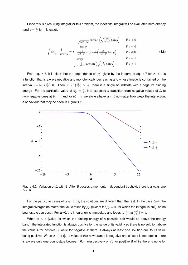
Since this is a recurring integral for this problem, the indefinite integral will be evaluated here already
(and d = ∆4 for this case).
∫dy
1
d− cos2 y=
−1√|d|2+|d|
arctan(√
|d||d|+1 tan y
)if d < 0
− tan y if d = 0
−1√d−d2 argtanh
(d√d−d2 tan y
)if d ∈]0, 1[
1tan y if d = 1
1√d2−d arctan
(√dd−1 tan y
)if d > 1
(4.8)
From eq. 4.8, it is clear that the dependence on pcF given by the integral of eq. 4.7 for ∆ < 0 is
a function that is always negative and monotonically decreasing and whose image is contained on the
interval ] − tan(pcF
2
), 0[. Then, if tan
(pcF2
)> π
B , there is a single boundstate with a negative binding
energy. For the particular value of pcF = π2 , it is expected a transition from negative values of ∆ to
non-negative ones at B = π and for pcF = π we always have ∆ < 0 no matter how weak the interaction,
a behaviour that may be seen in Figure 4.2 .
Figure 4.2: Variation of ∆ with B. After B passes a momentum dependent treshold, there is always one∆ < 0.
For the particular cases of ∆ ∈ 0, 4, the solutions are different than the rest. In the case ∆=4, the
integral diverges no matter the value taken by pcF (except for pcF = 0, for which the integral is null), so no
boundstate can occur. For ∆=0, the integration is immediate and leads to Bπ tan
(pcF2
)= 1.
When ∆ > 4 (value for which the binding energy of a possible pair would be above the energy
band), the integrated function is always positive for the range of its validity so there is no solution above
the value 4 for positive B, while for negative B there is always at least one solution due to its value
being positive. When ∆ ∈]0; 4[,the value of this new branch is negative and since it is monotonic, there
is always only one boundstate between ]0,4[ irrespectively of pcF for positive B while there is none for
41
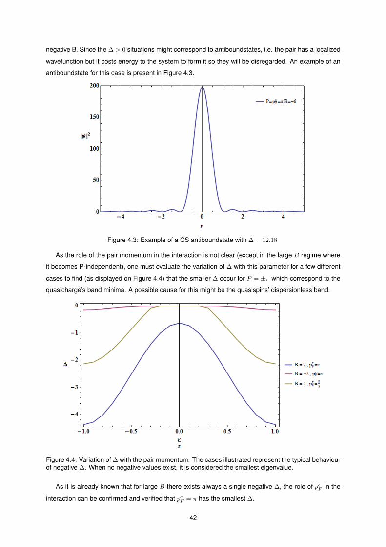
negative B. Since the ∆ > 0 situations might correspond to antiboundstates, i.e. the pair has a localized
wavefunction but it costs energy to the system to form it so they will be disregarded. An example of an
antiboundstate for this case is present in Figure 4.3.
Figure 4.3: Example of a CS antiboundstate with ∆ = 12.18
As the role of the pair momentum in the interaction is not clear (except in the large B regime where
it becomes P-independent), one must evaluate the variation of ∆ with this parameter for a few different
cases to find (as displayed on Figure 4.4) that the smaller ∆ occur for P = ±π which correspond to the
quasicharge’s band minima. A possible cause for this might be the quasispins’ dispersionless band.
Figure 4.4: Variation of ∆ with the pair momentum. The cases illustrated represent the typical behaviourof negative ∆. When no negative values exist, it is considered the smallest eigenvalue.
As it is already known that for large B there exists always a single negative ∆, the role of pcF in the
interaction can be confirmed and verified that pcF = π has the smallest ∆.
42

Figure 4.5: The variation of ∆ with pcF for various B shows a quasicharge filling threshold after whicha negative ∆ starts to emerge. As before, when no negative values exist, it is considered the smallesteigenvalue.
The dependence of ∆ with B can also be scrutinized to find there is always some B∗ for which exists
a single negative value of ∆. A more important feature is that for certain P and pcF there are also negative
values of ∆ for negative B.
To spot a boundstate, it is preferable to choose the parameter’s values that minimize ∆ and for
P = pcF = π, it shall be chosen B = 0, 8,−2 (which hold a ∆ = −1.13;−16.12;−0.16 respectively)
to clarify the nature of the eigenstates related to these values.
Figure 4.6: Square modulus of the pair’s wavefunction for the particle-hole Hubbard model.
43

(a) (b)
Figure 4.7: Square modulus of the pair’s wavefunction. The localized peak indicates a boundstate thatoccurs in the large B limit (high magnetic fields) while the spread wavefunction occuring in the repulsiveregime (negative B) does not provide a certainty about its nature.
While for B=8, the wavefunction decays extremely quickly and resembles a sharp localized peak, it
must be a boundstate, whereas for B=-2, the peaks are quite small and the decay is too soft to be claim
a boundstate nature. This is natural because the positive values of B correspond to large magnetic
fields and the negatives ones to a prevailing repulsive situation.
4.1.2 Case 2
Another simple CS binding can be evaluated using the π-momenta vertices instead. Since these vertices
do not conserve particle number, a pair of two vertices must be considered along with a pair of fermionic
propagators and another of bosonic ones to obtain a pattern to form the geometric sum and obtain a
Bethe-Salpeter equation for the vertex function as displayed on Figure 4.8.
Figure 4.8: Diagram associated with the Bethe-Salpeter equation for the 2nd CS case
Through the same algebraic processes, one obtains the same equation for the wavefunction but with
a potential for this 2nd case in the form:
CS case 2: V (q, k, P ) = −8ℵ(|q| − pcF )
∫dQ
2π
ℵ(|Q| − pcF )
∆− 2(cosQ+ 1)·(
cos k − cosQ− cosP + cos(Q+ P − k))×
×(
cos q − cos(Q)− cosP + cos(Q+ P − q))
(4.9)
44

As in this case the potential depends on ∆, an alternative way is necessary to obtain the binding
energies. Once again, using a discrete approximation, the wavefunction can be written as a column
vector where the value of its components ψk correspond to the weight of the function ψ at a given
momentum k. In this picture, one can define a N×N matrix Ξ(∆) defined by
Ξk,q(∆) =1
∆− 2(cos k + 1)
Vk,q(∆)
N(4.10)
and search for the ∆ that satisfies ψk = Ξk,q ψq. Since this corresponds to searching the eigenvalue 1,
one can simply define a function f(∆) = det(Ξ(∆)− I) and track its roots.
Figure 4.9: f’s dependence with ∆. The P=0 and the P=π situations overlap with each other.
The results in Figure 4.9 show that f(∆) is always negative for ∆ < 0 and at pcF = π a divergence
occurs at ∆ = 0. Unless the quasicharge band is empty, the divergence of f occurs at positive ∆. It is
clear from the figure the inexistence of any ∆ obeying the equation and so no boundstate can occur.
4.2 Quasicharge-Quasicharge binding
For the quasicharge-quasicharge interaction (CC case) using the vertices from the Hubbard model with-
out the additional terms considered, there are 3 simplest building blocks sharing the same peculiarity:
45

Figure 4.10: Diagram associated with the Bethe-Salpeter equation for the 1st CC case
Case 1: Γ(k, P −K) = i2∫∫
dQd$
(2π)2
dqdω
(2π)2U1(k, q,Q)U2(k, P, q,Q)D0(Q,$)
D0(k +Q− q,$ + E − ω)G0(q, ω)G0(P − q, E − ω)Γ(q, P − q) (4.11)
Figure 4.11: Diagram associated with the Bethe-Salpeter equation for the 2nd CC case
Case 2: Γ(k, P −K) = i2∫∫
dQd$
(2π)2
dqdω
(2π)2V1(k, P,Q)V2(q, P,Q)D0(Q,$)
D0(Q+ P − π,$ + E)G0(q, ω)G0(P − q, E − ω)Γ(q, P − q) (4.12)
For both cases the integration on $ is seen immediatly to be null because both the bosonic propaga-
tors have poles on the same side of the complex plane. Hence, one must try a more complex diagram
whose integration mixes the fermionic and bosonic propagators for the possibility of a non-null result.
The example considered is represented in Figure 4.12 and the pole condition is given by:
Case 3: Γ(k, P −K) = i3∫∫∫
dQ1dW1
(2π)2
dQ2dW2
(2π)2
dqdω
(2π)2U(k, q,Q1)V1(k, P,Q1, Q2)V2(k, q, P,Q1, Q2)
D0(Q1,W1)D0(Q1 + k − q,W1 + E1 − ω)D0(Q1 − P + k −Q2 − π,W1 −W2 − E2)
G0(q, ω)G0(Q2,W2)G0(P − q, E − ω)Γ(q, P − q)
(4.13)
46
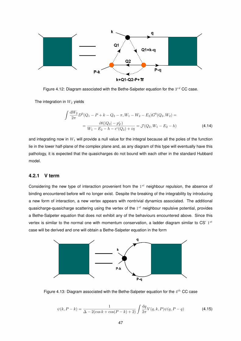
Figure 4.12: Diagram associated with the Bethe-Salpeter equation for the 3rd CC case.
The integration in W2 yields
∫dW2
2πD0(Q1 − P + k −Q2 − π,W1 −W2 − E2)G0(Q2,W2) =
=iℵ(|Q2| − pcF )
W1 − E2 − h− εc(Q2) + iη= J (Q2,W1 − E2 − h) (4.14)
and integrating now in W1 will provide a null value for the integral because all the poles of the function
lie in the lower half-plane of the complex plane and, as any diagram of this type will eventually have this
pathology, it is expected that the quasicharges do not bound with each other in the standard Hubbard
model.
4.2.1 V term
Considering the new type of interaction provenient from the 1st neighbour repulsion, the absence of
binding encountered before will no longer exist. Despite the breaking of the integrability by introducing
a new form of interaction, a new vertex appears with nontrivial dynamics associated. The additional
quasicharge-quasicharge scattering using the vertex of the 1st neighbour repulsive potential, provides
a Bethe-Salpeter equation that does not exhibit any of the behaviours encountered above. Since this
vertex is similar to the normal one with momentum conservation, a ladder diagram similar to CS’ 1st
case will be derived and one will obtain a Bethe-Salpeter equation in the form
Figure 4.13: Diagram associated with the Bethe-Salpeter equation for the 4th CC case
ψ(k, P − k) =1
∆− 2(cos k + cos(P − k) + 2)
∫dq
2πV (q, k, P )ψ(q, P − q) (4.15)
47

with the potential given by
V (q, k, P ) = VH(q, P ) cos(q − k) (4.16)
where H(q, P ) = ℵ(|q| − pcF )ℵ(|P − q| − pcF )− ℵ(pcF − |q|)ℵ(pcF − |P − q|).
A derivation similar to the CS’ case (the same procedure to get eq. 4.5) can be made to predict some
features of the interaction for some specific parameters. For P=π,
H(q, P = π) =
B]π−pcF ,pcF [ +B]−pcF ,−π+pcF [ if pcF >π2
−B]pcF ,π−pcF [ −B]−π+pcF ,−pcF [ if pcF <π2
(4.17)
where B]a,b[ = Θ(x − a) + Θ(b − x) − 1 and Θ(x) is the Heaviside function. Integrating in k the product
of H(q, P = π) cos k and both sides of eq. 4.15, and with some algebraic manipulations, one obtains
∆ = 4 + V(pcFπ
+sin 2pcF
2π− 1
2
)(4.18)
The result above tells that to obtain negative binding energies for P=π, it is necessary to have pcF as
low as possible and when pcF → 0, V > 8 must occur for this to happen (see Figure 4.14). Despite V
being a repulsive term, the fact that higher V provide smaller ∆ is because the pair’s binding comes from
the holes in the quasicharge Fermi sea. Further evidence of this may be seen in another possible case
where an analytical solution is possible, P=0. Integrating again the product of H(q, P = 0) by cos k (and
also H(q, P = 0) sin k ), and using simple trigonometric equalities, one arrives at
2 =
∫dk
2πH(q, P = 0)
V
∆− 8 cos2 k2
(4.19)
With the use of eq. 4.8, the ∆ < 0 solutions are given by
π
2V
√|∆|2 + 8|∆| = π
4− arctan
(√|∆||∆|+ 8
tanpcF2
)(4.20)
Since the potential is repulsive, to obtain negative binding energies the rightside of eq. 4.20 must be
positive, which occur no matter the quasicharge band filling because the rightside spans all R+. As an
increase in pcF will lower the rightside, at pcF = 0 it is minimal, and at this filling we get the dependence
∆ = 4
(√1 +
(V8
)2
− 1
)(4.21)
which corresponds to the blue line coming from the origin in Figure 4.14.
An important thing to notice is the appearance of an unexpected additional boundstate for higher
V. Although the role of pcF is clear (which can be seen directly from H(q, P )), the role of the remaining
parameters is not that clear. Evaluating eq. 4.15 by the method discussed above, it can be seen from
Figure 4.15 that the pair momentum that lowers the binding energy is P=0. An evaluation of the pair’s
wavefunction reveals that the always occurring possible boundstate is a spread wavefunction through all
real space (as seen in Figure 4.17) and must not represent a true boundstate. When the V threshold is
48

Figure 4.14: Variation of the binding energy with the repulsive potential. After a certain potential thresh-old, an additional binding energy appears.
Figure 4.15: ∆ variation with the pair momentum.
crossed and another negative binding energy occurs, the associated new boundstate is sharply centred
around the origin although for r = 0 the wavefunction vanishes as expected by Pauli’s exclusion principle
(while the old one remains unaltered). Hence the quasicharges only have a true boundstate after passing
a certain potential treshold.
49

Figure 4.16: ∆ variation with the Fermi momentum.
Figure 4.17: Square modulus of the wavefunction when there is only a single solution. The spreadwavefunction cannot be a boundstate.
4.3 Quasispin-Quasispin binding
4.3.1 Case 1
Finally, for the quasispin-quasispin case (SS case) the Bethe-Salpeter equation is
50

(a) (b)
Figure 4.18: Square modulus of the pair’s wavefunction for the CC case when another boundstateoccurs.
Figure 4.19: Diagram associated with the Bethe-Salpeter equation for the 1st SS case
ψ(k, P − k) =1
∆
∫dq
2πV (q, k, P )ψ(q, P − q) (4.22)
where the potential for the 1st case is
case 1: V (q, k, P ) = 8
∫dQ
2π
ℵ(|Q| − pcF )ℵ(|q − k −Q+ π| − pcF )− ℵ(pcF − |Q|)ℵ(pcF − |q − k −Q+ π|)∆ + 2(cos(q − k −Q)− cosQ)− ω1 − 2µ+ 4V
×
×(
cos(k +Q) + cos(Q− q)− cosQ− cos(q − k −Q))×
×(
cosQ+ cos(q − k −Q)− cos(P − q +Q)− cos(P − k −Q))
(4.23)
Since the potential exhibits the same problems of the 2nd CS case, a N×N matrix Ξk,q(∆) = 1∆Vk,q(∆)N
and a function f(∆) = det(Ξ(∆) − I) are defined and the same procedure is implemented. For P = 0
and P = π, the function f presents a region between ∆ = −15 and ∆ = −5 where all the solutions occur.
However the presence of some instabilities in this region may rise questions regarding the existence of
a true eigenvalue 1 for ψ = Ξψ.
51

Figure 4.20: Evolution of f(∆). There is an unstable region where boundstates may occur but it is notclear the exact corresponding values.
By calculating the eigenvalues of Ξ for ∆ in this region and considering only the eigenvalue closest
to 1, it can be observed (in Figure 4.21) that there are inumerous values of ∆ that are infinitely close to
1.
Figure 4.21: Distance of the closest eigenvalue to 1. The roots of f(∆) correspond indeed to the eigen-value 1.
Although the pair’s momentum role is not clear (the possible boundstate region is not noticeably
different; see Figure 4.22), the boundstate region is quite sensitive to the quasicharge’s filling and a
more empty band results in a region spanning smaller ∆ (Figure 4.23).
52

Figure 4.22: Evolution of f(∆) for P = π shows the roots in the same region of the case P=0.
(a) (b)
Figure 4.23: ∆’s momentum dependence for P=0 and pcF = π2 (a) and pcF = 0 (b).
As this type of interaction is much harder to analyze, another simple interaction between the qua-
sispins will be considered instead where the ∆ associated with the boundstates are found unequivocally.
4.3.2 Case 2
For the 2nd case, the potential is
Figure 4.24: Diagram associated with the Bethe-Salpeter equation for the 2nd SS case
53

V (q, k, P ) = 4
∫dQ
2π
ℵ(|Q| − pcF )ℵ(pcF − |k +Q− q|)− ℵ(pcF − |Q|)ℵ(|k +Q− q| − pcF )
ω1 − h+ 2(cosQ− cos(Q+ k − q))×
×(
cos(k +Q) + cos(Q− q)−B)(
cos(P − q +Q) + cos(P − k −Q)−B)
(4.24)
where ω1 is the frequency of a single quasispin entering the diagram. Due to the possibility of a vanishing
denominator, the value of ω1 − h was set to 2.1, where no divergences of the potential were noticed.
Since this potential does not depend on ∆, the initial eigenvalue analysis can be used. It was found that
P=0 is the pair’s momentum that minimizes the binding energy as seen in Figure 4.25.
(a) SS2 ∆’s P dependence for pcF = π2
and B=-4(b) SS2 ∆’s P dependence for pcF = π
2and B=0
(c) SS2 ∆’s P dependence for pcF = π2
and B=2
Figure 4.25: ∆’s momentum dependence for various B. The case of the particle-hole defined Hubbardmodel (B=0, which corresponds to (b)) distinguishes itself from the others due to the existence of threeminima as a function of the pair’s momentum.
Contrasting with the previous cases, the SS2 case is characterized by inumerous possible bound-
states. For contention reasons, only the smaller ∆ wil be considered in the following analysis. Since
the bands have different variations with the parameters, the ∆ variation presented might have spikes
provenient from band transitions. Since, when B = 0, more than one minimum exists, and since this
case corresponds to the standard Hubbard model, it will receive an additional attention.
(a) Smallest ∆’s momentum dependence for various B and pcFfor the SS case
(b) Smallest ∆’s momentum dependence for various B < 1 forthe SS case
Figure 4.26: Smallest ∆’s momentum dependence for various B and pcF . It can be noted that the twoadditional local minima appear when |B| < 1 and become global minima only when B=0.
The quasicharge filling that minimizes ∆ is π2 and larger B also minimizes it as can be seen in Figures
4.27 and 4.28 respectively.
54

Figure 4.27: Smallest ∆’s variation with pcF , exhibiting a minimum at π2
Figure 4.28: Smallest ∆’s variation with B
The search for the boundstate when P=0, pcF = π2 and B=4, results in a smallest ∆ with the value of
-85,71 and despite the very low binding energy, the wavefunction is too spread to be a boundstate (as
can be seen in Figure 4.29) and tends to accumulate in the extremes of the system.
However for the particle-hole Hubbard model, the states with the minimum ∆ (∆ = −8.75) exhibit a
very fast decay, and confirm their true boundstate nature. Assuming that at least a portion of the states
with negative ∆ have a similar behaviour to this, the quasispins have inumerous true boundstates and
tend to bind toghether in unidimensional systems.
55

Figure 4.29: Square modulus of the pair’s wavefunction. The spread wavefunction does not give rise toa boundstate.
(a) Square modulus of the SS pair’s wavefunction. (b) Square modulus of the SS pair’s wavefunction.
Figure 4.30: Square modulus of the SS pair’s wavefunction. The fast decaying peaks foretell the confir-mation of a boundstate.
A brief remark about the three cases must be made: in the particle-hole Hubbard model there exists
inumerous boundstates and when turns on the other types of interaction they destroy their localized
nature and become unbound. These true boundstates start to appear when B < 1, where inverted
bands (the bands corresponding to the binding energy as a function of P) are also present.
4.4 The role of propagator corrections
The pseudoparticles considered previously were simply the pseudoparticles from the non-interactive
system. To account for the correct particles’ interaction in the medium, one must consider the propa-
gators of the full interacting system. This is done by considering all the interactions correcting the bare
propagators, which will be gathered in the self-energy Σ and will correct the pseudoparticles’ energy
bands.
56

Through the Dyson’s equation, the correction to the bosonic propagator will be
D(k, ω) =1
ω −$(k)− Σ?(4.25)
Since an exact calculation of the proper self-energy Σ? is too complicated, it will be approximated
here by the 1st order terms contributing to the proper self-energy. Through the use of
∫dωeiωηG0(k, ω) = iℵ(pcF − |k|) (4.26)
one can see that the approximation for Σ? for the dressed bosonic propagator is
Σ(1)(k) = i
∫∫dq
2π
dω
2πeiωηG0(q, ω)
(2 cos(k + q) + 2− 2B
)= 2(1−B)
(pcFπ− 1)− 2
πcos k sin pcF (4.27)
and since bosons do not possess a Fermi surface, by eq. 4.26 one can see that the U0 interaction
provides a null correction to the fermionic propagator. The major role of the proper self-energy is to
provide a dispersive band to the quasispins but the previous calculations remain valid apart from an
addition to the band energies of Σ?. This makes the correction to Bethe-Salpeter equation for the CS
case
ψk =1
∆− 2(cos k − 1π sin(pcF ) cos(P − k) + 1 + 1
π sin(pcF ))
∫dq
2πVkqψq (4.28)
As the quasicharge band filling role is now more prominent, an analysis to the ∆ dependence with it
for the 1st CS case considered reveals that the corrections introduced by the dressing of the propagators
is simply a shift on the band filling threshold for which negative ∆ start to occur (see Figure 4.31). The
analysis on the P dependence did not reveal anything new. As the smaller ∆ occur for a filling that
cancels the self-energy correction, the boundstate found for this case remains unaltered.
Figure 4.31: ∆’s quasicharge Fermi momentum depence for the dressed propagator.
57

For the 2nd CS case, no boundstates were found again (see Figure4.34).
Figure 4.32: f(∆) has no roots so no possible boundstates can occur.
The dressed propagator is specially important in the SS case because introduces a non-flat band
for the quasispins and also because the quasicharge bandfilling that minimized ∆ is also the one that
maximizes the self-energy contribution. The Bethe-Salpeter equation for the SS case is
ψk =1
∆ + 2π sin(pcF )(cos k + cos(P − k)− 2)
∫dq
2πVkqψq (4.29)
and despite the existence of new terms for the P dependence, this is not altered (see Figure 4.35)
(a) (b)
Figure 4.33: ∆ variation with the pair’s momentum.
The corresponding wavefunctions analysed previously are now modified such that now one of the
previous boundstates is a spread function and the second becomes two localized separate peaks.
For the CC case, the propagator corrections must come from the 1st neighbour interaction potential
58

Figure 4.34: Square modulus of the pair’s wavefunction for the dressed propagator. The spread wave-function does not give rise to a boundstate.
(a) Square modulus of the SS pair’s wavefunction. (b) Square modulus of the SS pair’s wavefunction.
Figure 4.35: Square modulus of the SS pair’s wavefunctions for the dressed bosonic propagators. Whilein one case the previous boundstate now gives rise to a spread wavefunction, the other exhibits a fastdecaying peaks that foretell the confirmation of a boundstate.
and for this case, the proper self-energy will be taken to be
Σ(1)(k) = i
∫∫dq
2π
dω
2πeiωηG0(q, ω)
(2 cos(k + q) + 2− 2B
)= V
(1− pcF
π
)− V
πcos k sin pcF (4.30)
which leads to the Bethe-Salpeter equation for this case
ψk =1
∆− 2(cos k + cos(P − k) + 2)− Vπ sin(pcF )(cos k + cos(P − k)− 2)
∫dq
2πVkqψq (4.31)
As before, the role of the dressed propagator is simply to shift the threshold for which the true
boundstate occurs.
59

Figure 4.36: ∆ variation with pcF for the dressed propagator.
60
Chapter 5
Dimensional Crossover
Since the unidimensional case presents some particular features provenient from the dimensionality
restrictions, it is interesting to see how the transition to the twodimensionality affects the peculiar physics
of this type of systems. For this, it is considered that the unidimensional chains may couple with each
other through an interaction with a tunable parameter α ∈ [0; 1] such that α = 0 corresponds to the
uncoupled unidimensional chains and α = 1 to the twodimensional square lattice. Futhermore, it is
considered that the interchain coupling is simply a hopping to the nearest site of another chain with the
hopping parameter α. This leads to an additional term in the Hamiltonian (besides the increase of the
dimension) given by
Hextra = −α∑r,σ
c†x,y,σcx,y+δ,σ + c†x,y+δ,σcx,y,σ (5.1)
Taking the preceding path, the Hamiltonian is rewritten in terms of an Ostlund-Granath transformation
for the 2D case that can be taken as:
c~r = c†↑,~r(1− n↓,~r) + (−1)x+yc↑,~rn↓,~r
q+~r =
(c†↑,~r − (−1)x+yc↑,~r
)c↓,~r
q−~r =(q+~r
)†qz~r = 1
2 − n↓,~r
(5.2)
The phase factor (−1)x+y was chosen in the attempt to retain the symmetries preserved by the choice
of (−1)r in the unidimensional case. If one wants the symmetries to appear only for the unidimensional
chains (or a privileged direction in space) a factor of (−1)x may be chosen instead. However this
choice will affect only the π-momenta vertexes. After the approximation with the Holstein-Primakoff
transformation, the Hamiltonian takes the previous form with an enlargment of the dimension and the
additional terms:
T extra0 = α∑x,y
(a†x,yax,y+δ + a†x,y+δax,y + 1)(c†x,ycx,y+δ + c†x,y+δcx,y) (5.3)
T extraπ = α∑r
(−1)x+y(nx,y + nx,y+δ − a†x,yax,y+δ − a†x,y+δax,y)c†x,yc†x,y+δ (5.4)
61

Since the twodimensional Hamiltonian considered presents the same structure of the unidimensional
case, it follows directly that the correction to the the fermionic propagator (the bosonic remains unaltered)
is
Fermionic propagator: G0(~k, ω) =Θ(ε(k)− EF )
ω − 2(cos kx + α cos ky + u4 ) + iη
+Θ(EF − ε(k))
ω − 2(cos k + α cos ky + u4 )− iη
(5.5)
The Θ function for the energy was used because the Fermi momentum is not easily expressed for a
general α. Note that Θ depends on α through the expression for the fermionic band . The correction for
U0 is
U0 vertex: 2[
cos(k′′ + k1) + cos(k′′ − k2) + α(
cos(k′′ + k1) + cos(k′′ − k2))−B
](5.6)
For contention reasons, only the quasicharge-quasispin interaction will be considered. The Bethe-
Salpeter equation for the 1st CS case in two dimensions is
ψ~k =1
∆− 2(cos kx + α cos ky + 1 + α)
∫d~q
(2π)2V~q,~kψ~q (5.7)
and the potential given by
CS 2D case 1: V~q,~k = 2Θ(ε(k)−EF )[
cosPx+α cosPy+cos(Px−kx−qx)+α cos(Py−ky−qy)−B]
(5.8)
The method used is extended for the twodimensional case by simply enlarging the vectors ψk (with
the new size being N2) and matrices (with the new size being N2 × N2) involved, such that each set
of N consecutive components corresponds to a fixed momentum along x while the y component runs
over all possibilities. For economic reasons, N will be taken to be 100. Beginning with the values that
minimize ∆ for the unidimensional case, turning on the interchain coupling will lower the binding energy
but no additional boundstates appear as seen in Figure 5.1.
Figure 5.1: ∆ variation with the interchain hopping parameter α for Py = π and B=0. It is observed thatthe qualitative behavior is not altered in the transition to the twodimensionality.
62

The Fermi energy considered in all cases was at the quasicharge’s band minima in order to maximize
the potential. Other cases with a not so extreme filling were also analysed but did not present any
meaningful qualitative change. The role of Py is also seen to be too similar to the role of Px as seen by
its variation in Figure 5.2.
(a) (b)
Figure 5.2: ∆ variation for Py = 0 (a) and Py = π2 (b). ∆’s pace with Py resembles the pace with Px.
The results on Figure 5.2 may seem to tell that the binding vanishes when reaching the twodimen-
sionality, but the results are for pair’s momenta with a component along the chain much bigger than the
component perpendicular to the chain. Comparing with Figure 5.1, one can see that the boundstate
formed must not have a privileged propagation direction.
Although the results above are only for the particle-hole Hubbard model, the influence of B is not sig-
nificant. For positive B the binding energy is almost α-independent while for negative B the dependence
is quite strong but a single boundstate appears no matter the α taken.
(a) (b)
Figure 5.3: ∆ variation for negative (a) and positive (b) B.
Despite the inclusion of self-energies in the bosonic propagator had not lead to any significant change
in the unidimensional case, the anisotropy presents a complicated deformed band and could provide
interesting results. For the twodimensional case the approximation to the proper self-energy will be
given by
Σ?(k) ≈ −∫
dq
2πΘ(EF − ε(~q))
[2 cos(kx + qx) + 2 + 2α+ 2α cos(ky + qy)− 2B
](5.9)
and with it the Bethe-Salpeter equation presents the same expression as before but with an additional
63

quasispin band contribution from Σ?.
(a) (b)
Figure 5.4: ∆ variation for Py = 0 (a) and Py = π (b) including of self-energies in the bosonic propagator.
However, the results show that no corrections are made to the lower ∆ (see Figure 5.4). Contrarily
to the expected of the transition to the twodimensionality, no new physics were found. New phenomena
might be lurking out from the non-conserving momentum interactions but due to the problems associated
with these (primarly the binding energy dependent potential), their analysis would be too time consuming
and it shall be postponed.
64

Chapter 6
Epilogue
In the work developed in this thesis, it was derived the pseudoparticle energy band, the phase shifts and
the relation between pseudomomenta and rapidities for the Heisenberg model and for the Kondo model.
These results are useful for obtaining exponents that can be compared with experiments such as the
dynamical spin structure factor.
This lays the ground for a future calculation of the dynamical structure factor for the Kondo model that
can be obtained in a manner analogous to the Heisenberg model. Knowing the physics involved, they
must be similar apart from an impurity term. Another possible correlation function to be calculated is the
electronic spectral function. Since for the free electron gas it is simply a δ-function spectral function, it
would be interesting to see what is the impurity’s role. This question has yet not been resolved.
In the study of the scattering between the quasicharges and quasispins was found that the qua-
sicharges and quasispins form boundstates in a vast region of the parameter space. This binding was
unexpected since in one dimension there are several examples of fractionalization and the operators
representing the pseudoparticles decouple. On the other hand, quasicharges do not bind with each
other in the particle-hole Hubbard model but they start to do so when a first neighbour interaction is
considered. This absence of binding is a good outcome since the transformation proposed by Ostlund
and Granath was made with the intent of spliting the quasicharge sector, but this lack of binding is a
feature provenient from the Holstein-Primakoff transformation of the quasicharges and it is independent
of the dimension. The quasispins always bind with each other and possess inumerous boundstates.
These boundstates found may be originated by the use of the ferromagnetic representation. The uni-
dimensional ferromagnetic Heisenberg model has one boundstate below the two-particle continuum for
each momentum value [6]. Since in our case the spin coupling is null, the corresponding situation is a
collapse of the continuum of states into a single line coinciding with the boundstates. Hence, it migh
be expectable the appearance of the boundstates in the quasispin-quasispin scattering due to the some
high degeneracy. The role of propagator corrections was also analysed and it was not found any signifi-
cant change in the binding.
Finally, the transition to the bidimensionality did not show any new phenomena, being a continuation
of the unidimensional case. As the quasicharges and quasispins already bind in one dimension, the
65

appearance of a boundstate in two dimensions is not surprising. Although the analysis was done for
the simplest quasispin-quasicharge interaction, it is not expected that the analyzis of other cases reveal
any differences. An undermining problem was the flat quasispin band. The approach taken with the lin-
earization of the Holstein-Primakoff transformation lead to an effective Hamiltonian with the assumption
that the quasispin density was negligible. However this is a somewhat drastic approach and there may
be other ways to overcome the problem. As the Jordan-Wigner transformation is much more reliable
for the quasispin interaction with the quasicharges, the dispersionless quasispin band problem may be
bypassed by the simple addition of an electronic spin interaction term J ~Sr · ~Sr+δ instead of the other
terms added to the Hubbard Hamiltonian. This interaction might provide a momentum dependent band
that will outline a well-defined fermionic propagator for the quasispins. This will also provide a non-trivial
interaction between quasicharges.
66

Bibliography
[1] Kim et al., Distinct spinon and holon dispersions in photoemission spectral functions from one-
dimension SrCuO2, Nature Physics, 2
[2] S. Ostlund, M. Granath, Exact Transformation for Spin-Charge Separation of Spin-1/2 Fermions
without Constraints, Physical Review Letters, 96, 066404 (2006)
[3] Natan Andrei, Integrable models in condensed matter systems, ICTP Summer course.
[4] Franz Gross, Relativistic quantum mechanics and field theory, WILEY-VCH Verlag GmbH and Co.
KGaA, Weinhem (2004)
[5] J. Smakov, A. Chernyshev, S. White, Binding of Holons and Spinons in the One-Dimensional
Anisotropic t-J Model, PRL, 98, 266401 (2007)
[6] D.C. Mattis, The theory of magnetism made simple,World Scientific (2008)
[7] J.M.P. Carmelo, P.D. Sacramento, Finite-energy Landau liquid theory for the one-dimensional Hub-
bard model: Pseudoparticle energy bands and degree of localization/delocalization, Physical Re-
view B, 68 (2003)
[8] J. Carmelo, P. Horsch, P.A. Bares, A.A. Ovchinnikov, Renormalized pseudoparticle description of
the one-dimensional Hubbard model thermodynamics, Physical Review B 44, 18 (1991)
[9] J.M.P. Carmelo, P. Horsch, A.A. Ovchinnikov,Static properties of one-dimensional generalized Lan-
dau liquids, Physical Review B 45, 14, 7899 (1992)
[10] J.M.P. Carmelo, L.M. Martelo and P.D. Sacramento, One and two-electron spectral function line
shapes in the vicinity of the upper-Hubbard bands lower limits, J. Phys. Cond. Matt. 16, 1375
(2004)
[11] J.M.P. Carmelo, K. Penc, L. M. Martelo, P. D. Sacramento,J. M. B. Lopes dos Santos, R. Claessen,
M. Sing and U. Schwingenschlogl, One-electron singular branch lines of the Hubbard chain, Euro-
physics Letters 67, 233 (2004)
[12] R.G. Pereira, K. Penc, S.R. White, P.D. Sacramento, J.M.P. Carmelo, Charge dynamics in half-filled
Hubbard chains with finite on-site interaction, Physical Review B 85, 165132 (2012)
67

[13] Holger Frahm and V. E. Korepin, Critical exponents for the one-dimensional Hubbard model, Phys-
ical Review B 42,10553 (1990)
[14] B.A.Bernevig, D. Giuliano, R.B. Laughlin, Coordinate representation of the two-spinon wave func-
tion and spinon interaction in the Haldane-Shastry model, Physical Review B 64, 024425 (2001)
[15] P.D.Sacramento, Y.C.Li, S.J. Gu, J.M.P.Carmelo, Spinon and η-spinon correlation functions of the
Hubbard chain, EPJ B 64, 024425 (2013)
[16] C.F. Coll, Excitation spectrum of the one-dimensional Hubbard model, Physical Review B 9, 5
(1974)
[17] H.A. Bethe, Zur Theorie der Metalle, Z.Phys. 71, 205 (1931)
[18] D. Braak, N. Andrei, Physical picture of the gapped ecitation spectrum of the one-dimensional
Hubbard model, Nuclear Physics B 542, 551-580 (1999)
[19] J.M.P. Carmelo, H.Q.Lin, SU(2) to U(1) microscopic transition in the Heisenberg chain, Modern
Physics Letters B 7, 21, 1387-1396 (1993)
[20] L.D. Faddeev, L.A. Takhtajan, What is the spin of a spin wave?, Physics Letters 85A, 6, 7 (1981)
[21] Alexander L. Fetter and John Dirk Walecka, Quantum theory of many-particle systems, McGraw-Hill
Book Company
[22] S. Lee, S. Salk, Holon pairing instability based on the Bethe-Salpeter equation obtained from the
t-J Hamiltonians of both U(1) and SU(2) slave-boson symmetries, Physical Review B 66, 054427
(2002)
[23] D.Bozi ,J. M. P. Carmelo, K. Penc and P. D. Sacramento, The TTF finite-energy spectral features
in photoemission of TTF–TCNQ: the Hubbard-chain description, J. Phys.: Condens. Matter 20,
022205 (2008)
[24] F. D. M. Haldane, Luttinger liquid theory of one-dimensional quantum fluids. I. Properties of the
Luttinger model and their extension to the general 1D interacting spinless Fermi gas, J. Phys. C:
Solid State Phys. 14, 2585 (1981)
[25] N. Andrei, Diagonalization of the Kondo Hamiltonian, Phys. Rev. Lett. 45, 379 (1980)
[26] P.B. Wiegmann, Pis’ma Zh. Eksp. Teor. Fiz. 31, 392 (1980)
[27] K.J.B.Lee, PhD Thesis, Temple University (1990)
[28] J. Carmelo et. al., Strongly correlated systems, coherence an entanglement, World Scientific,
(2007)
[29] N.Peres, A fısica dos materiais unidimensionais,unpublished.
[30] J. Voit, One dimensional Fermi Liquids, http://arxiv.org/abs/cond-mat/9510014
68

[31] C.Varma, Z.Nussinov, W. van Saarloos, Singular or non-Fermi liquids, Physics Reports, 361, 267-
417 (2002)
[32] J. Finney, U. Steigenberger, Neutrons for the future, Physics World 10,12,27 (1997)
[33] M. Sing et. al, Electronic structure of the quasi-one-dimensional organic conductor TTF-TCNQ,
http://http://arxiv.org/abs/cond-mat/0304283v1
[34] Conrad Sanderson, Armadillo: An Open Source C++ Linear Algebra Library for Fast Prototyping
and Computationally Intensive Experiments,NICTA,(2010)
[35] M. Takahashi, Thermodynamics of the one-dimensional solvable models, Cambridge University
Press (1999)
[36] F.H.L. Essler et al., The one-dimensional Hubbard model, Cambridge University Press, (2005)
[37] F.H.L.Essler, V.E.Korepin, Physic Review Letters 72, 908 (1994)
[38] J.M.P. Carmelo, P.D.Sacramento, arXiv: 1211.6073
[39] J.M.P. Carmelo, Nuclear Physics B 824, 452 (2010)
69

70

Appendix A
Zero temperature diagrammatic rules
for the extended Hubbard model
Most problems in physics involving interactions do not have a simple or even clear way to obtain exact
solutions (if any exist). A way to contour this situation is through perturbation approaches where one
starts from the solutions of the non-interacting system (supposing that all is known about the non-
interacting system) and interactions are treated as perturbations that are included iteratively hoping
that the approximate solution approaches the exact solution.
For interactions that are switched on adiabatically so H = H0 + e−ε|t|HI , where ε is an infinitesimal
small amount so the system is in the non-interactive groundstate |Φ0〉 for t → ±∞, one can obtain any
eigenstate of the interacting system through the time evolution operator by
|Ψs(t)〉 = Uε(t, t0)|ΨH(t0)〉 = Uε(t0,−∞)|Φ0〉 (A.1)
and obtain the time evolution throught
Uε(t, t0) =
+∞∑n=0
(−i)n
n!
∫ t
t0
dt1...
∫ t
t0
dtne−ε
∑j |tj |T
[ n∏j=1
HI(tj)
](A.2)
An important tool to probe the interacting system’s observables is the groundstate Green’s function
defined by
iG(x, t; y, t′) = 〈Ψ0|T[ψ(x, t)ψ†(y, t′)
]|Ψ0〉 (A.3)
and where the groundstate eigenstates are normalized and the time ordering for a field ψ is defined by
T [ψ(x, t), ψ†(x′, t′)] =
ψ(x, t)ψ†(x′, t′) for t > t′
±ψ†(x′, t′)ψ(x, t) for t < t′(A.4)
Any physical quantity of the interacting system can be evaluated by the use of the Green’s function
71

by
〈O(x)〉 = ±i limt′→t+
limy→x
O(x)G(x, t; y, t′) (A.5)
where O is the second-quantized operator associated with O. Despite the exact Green’s function is not
easily calculated, an approximation scheme can be built through the adiabatic evolution of the non-
interacting groundstate to the interactive groundstate by
iG(x, y) =
+∞∑n=0
(−i)n
n!
∫ +∞
−∞dt1...
∫ +∞
−∞dtn〈Φ0|T
[(n∏j=1
HI(tj)
)ψ(x)ψ†(y)
]|Φ0〉 (A.6)
This well-defined expansion is possible due to Gell-Mann and Low’s theorem that states that if the
quantity
limε→0
Uε(0,−∞)|Φ0〉〈Φ0|Uε(0,−∞)|Φ0〉
≡ |Ψ0〉〈Φ0|Ψ0〉
(A.7)
exists in all orders in perturbation theory than the rightside of the expression above is an eigenstate of
the Hamiltonian. The Wick’s theorem allows the expression of a product of creation and annihilation
operators to be expressed in terms of pairs of creation and annihilation operators. Thus the nth order
Green’s function can be obtained through combinations of n zero order Green’s functions.
The Hamiltonian for the extended Hubbard model considered is
H =∑r
(1 + a†r+δar + a†rar+δ) (c†rcr+δ + c†r+δcr) +∑r
(−1)r(a†r+δar+δ + a†rar − a†r+δar − a
†rar+δ)·
· (c†rc†r+δ + cr+δcr) + h
∑r
a†rar + (η − u
2+h
2− 2V )
∑r
c†rcr + (4V − h+ u− 2η)∑r
a†rarc†rcr+
+ V∑r
c†r+δcr+δc†rcr (A.8)
A direct expression for the groundstate Green’s function in frequency and momentum space is pos-
sible throught the relation
Θ(t− t′) = −∫ +∞
−∞
dω
2πi
e−iω(t−t′)
ω + iη(A.9)
and performing the Fourier transform of the Green’s function, one arrives at
G0(~k, ω) =ℵ(k − pF )
ω − ε(~k)
+ iη+ℵ(pF − k)
ω − ε(~k)− iη(A.10)
for the fermions, while the bosonic propagator (coined as D0 to distinguish it from the fermionic one) is
D0(~k, ω) =1
ω −$(~k)
+ iη(A.11)
A remark must be made about attaining the bosonic propagator. In the absence of magnetic field,
the quasispin population is not well-defined in momentum space due to its momentum independent zero
energy. However, in the presence of an external magnetic field ($(~k) = h), and at exactly T=0, the
system can be considered ordered (in the sense that no quasispins exist at the groundstate) and all
excitations can be constructed from this state.
72

The exact Green’s function can be obtained by considering the series in eq. A.6 and the effects of the
potential can be retrieved by the corrections made on the non-interacting Green’s function. Considering
in first place the quasicharges propagator and the effects of the instantaneous potential between a qua-
sicharge and another Ux = 12V (δr′,r+δ+δr′,r−δ) (from
∑r,r′ Ux(r, r′)c†r′c
†rcrcr′ ), the 1st order propagator
is given by:
G(1)(x, y) =i
2
∫∫dzdwUx(z, w)
[G0(x, y)(G0(w,w)G0(z, z)−G0(z, w)G0(w, z))
+G0(x, z)(G0(z, w)G0(w, y)−G0(z, y)G0(w,w))
+G0(x,w)(G0(w, z)G0(z, y)−G0(w, y)G0(z, z))]
(A.12)
The first two terms correspond to disconnected diagrams. The exact Green’s function can be factorized
in the product of a sum of connected diagrams and a sum of disconnected corrections. The sum of
all the disconnected corrections is equal to 〈Φ0|S|Φ0〉=1 because of the normalization chosen, so their
contribution can be disregarded. The remaining propagator corrections can be written in frequency and
momentum space as
G(1)(k, ω) = G0(k, ω)(∑
q
iUx(k− q)G0(q, ω))G0(k, ω)−G0(k, ω)
(∑q
iUx(0)G0(q, ω))G0(k, ω) (A.13)
with the diagrammatic correspondence in Figure A.1
Figure A.1: 1st order contribution to the fermionic propagator of the 2nd neighbour interactions. Forcompactness the diagrams will be agglutinated.
Since the series possess a pattern, one might retrieve a set of rules for evaluating any term of it from
the 1st order contribution.
The nth order contribution is obtained by:
•Drawing all topologically distinct connected diagrams with n vertices.
•Associate a momentum and an energy to each propagator represented by the corresponding line and
ensure that the total incoming momentum and energy at each vertex are the same that the outcoming
momentum and energy (only for interactions conserving the momentum; when this does not happen the
excess momentum created in the vertex must be transported in the outcoming lines).
•Assign a factor of iU at each vertex, where U is the interaction intensity.
73

•Integrate over the internal independent degrees of freedom.
•For each fermion loop beginning and ending in the same vertex affix a eiωη factor and if the loop closes
on itself an extra (-1) factor.
For the contribution of the U0 interaction term, it will be analysed its contribution to the bosonic propa-
gator instead. The interaction has a density-density component just as the potential Ux for the interaction
between two fermions, so the only connected part of 〈Φ0|T[a†r′c
†r′craraxa
†y
]|Φ0〉 isD0(x, r)G0(r, r′)D0(r, y).
This is simply a Fock term for the bosons. The remaining term is 〈Φ0|T[a†rc†r′cr′araxa
†y
]|Φ0〉 which in turn
has also just one connected diagrammatic component of D0(x, r)G0(r′, r′)D0(r, y) corresponding to a
Hartree term. This makes
D(1)(k) = D0(k)D0(k)i∑q
[2 cos(k + q) + 2− 2B]G0(q) (A.14)
and a diagrammatic representation similar to Figure A.1. The same rules above are valid and the general
form of the interaction term for U0 can be extrapolated to be
U0(q, k1, k2) = 2[
cos(q + k1) + cos(q − k2)−B]
(A.15)
To obtain the effects of the remaining interactions, one cannot consider simply the 1st correction to
the propagator because they do not conserve particle number and hence one must move on to the 2nd
order. The term to be evaluated is now
∑r,r′
∑z,z′
(−1)r+zV (r, r′)V (z, z′)〈Φ0|T[(a†rar + V (r, r′)a†r′ar′ − V (r, r′)a†r′ar − V (r, r′)a†rar′)
(a†zaz + V (z, z′)a†z′az′ − V (z, z′)a†z′az − V (z, z′)a†zaz′)(c†rc†r′ + cr′cr)(c
†zc†z′ + cz′cz)cxc
†y
]|Φ0〉 (A.16)
where V (r, r′) = 12 (δr′,r+δ + δr′,r−δ). The full sum will lead to a propagator in momentum space of
G(2)(k) = 32∑q,Q
cos2 k(
cos(q)− 1)(
cos(Q)− 1)G0(k)D0(q)G0(k + π)D0(Q)G0(k) (A.17)
A thorough inspection reveals that the term 4 cos k(cos q − 1) is provenient from a single interac-
tion term and that the factor of two arises from a difference of V?(r, r′) − V?(r′, r) provenient from the
antissymetric properties of the quasicharge operators. This has a diagrammatic correspondence of an-
tissymetrized conections between the fermionic lines connecting the π-vertices. Since V+(q, k1, k2) and
V−(q, k1, k2) are antissymetric in the fermion momenta, one may just take one link and multiply a factor
of 2. These vertices are found to yield the interaction strenght
V+(q, k1, k2) = 2(cos k2 − cos k1 + cos(k1 − q)− cos(k2 − q))
V−(q, k1, k2) = 2(cos k1 − cos k2 + cos(k2 + q)− cos(k1 + q)) (A.18)
74

One can also encompass all corrections of the interactions into a self-energy term Σ. The equation
for the full propagator is then
G(k, ω) = G0(k, ω) +G0(k, ω)Σ(k, ω)G0(k, ω) (A.19)
This self-energy can be decomposed in the proper self-energy Σ?, which contains just the terms of
non-repeating diagrammatic patterns dressing the propagator. This makes
Σ = Σ?+∞∑j=0
(G0Σ?
)j(A.20)
Its substitution into A.19 will lead to Dyson’s equation
G = G0+∞∑j=0
(Σ?G0
)j= G0 +G0Σ?G (A.21)
The generalization to obtain the scattering matrix is immediate. Through the diagram representing
the interaction, one just simply has to affix a propagator for each incoming and outgoing particles and
the vertices and integrations characteristic of the interaction.
75

76