Embed Size (px)
Citation preview
Forecasting Traffic and Balancing Load for Quality DrivenLTE Networks
Miguel Aires Barros Monteiro
Thesis to obtain the Master of Science Degree in
Electrical and Computer Engineering
Supervisors: Doctor Antonio Jose Castelo Branco RodriguesDoctor Pedro Manuel de Almeida Carvalho Vieira
Examination Committee
Chairperson: Doctor Jose Eduardo Charters Ribeiro da Cunha SanguinoSupervisor: Doctor Antonio Jose Castelo Branco Rodrigues
Members of the Committee: Doctor Francisco Antonio Bucho Cercas
November 2016


Acknowledgments
First and foremost, I would like to thank my parents for all the support and encouragement they have
given me over the years, none of this would be possible without them. I would like to thank my siblings,
grandparents, cousins, aunts and uncles for being there when needed.
I would also like to thank my supervisor Professor Antonio Rodrigues and co-supervisor Professor
Pedro Vieira, for the insight, knowledge and support they provided during the course of this project. I
would like to thank Celfinet for the opportunity of doing my thesis in a company environment, specially
Eng. Andre Martins for providing valuable insight and support throughout my internship.
Last but not least, to all my friends and colleagues that helped me through my time in Tecnico, by
collaborating in projects and studying, or just being great friends overall. Specifically, Antonio Mendes,
Bernardo Jubert, Bernardo Marques, Daniel Sousa, Hugo Pereira, Hugo Silva, Jessy Neves, Joao
Franco, Joao Galamba, Joao Rocha e Melo, Jose Teixeira, Manuel Avila de Melo, Manuel Beja da
Costa, Manuel Ribeiro, Miguel Rodrigues, Nuno Sousa, Pedro Figueiredo and Ruben Borralho.

Abstract
With the current increase in network traffic in radio networks, it is now more important than ever to
manage this traffic efficiently in order to utilise the available network resources intelligently. The goal of
this thesis is to provide means for the operators to optimise their networks regarding the management
of load across the network.
This thesis proposes a two part approach to load management, an autonomous load balancing
algorithm in conjunction with a traffic forecasting methodology.
The proposed load balancing algorithm works in closed loop where each cell measures its load and
its neighbors load in order to adjust its handover parameters to offload traffic to other cells. Several sim-
ulations were run in order to validate the concept, the utilisation of this method decreased the average
number of unsatisfied users in a network up to 4%, depending on the network configuration. The simu-
lations were run using the MATLAB Vienna LTE System Level Simulator [1], which was heavily modified
for this work.
The forecasting tools and methodologies discussed in this work were mostly taken from the field of
economics and were shown to work extremely well when used to forecast network traffic, whether it be
data or voice. Some of the proposed techniques were shown to predict network traffic two months in
advance with a median error across 86 cells of just 14%.
This approach shows the potential of reducing the amount of wasted network resources and increase
savings for the operator.
Keywords
LTE; SON; Load Balancing; Traffic Forecasting.
iii


Resumo
Com o atual aumento do trafego nas redes de telecomunicacoes, e hoje mais importante que nunca
gerir este trafego de forma eficiente de maneira a usar os recursos existentes na rede inteligentemente.
Este trabalho tem como objetivo apresentar formas de os operadores moveis otimizarem as suas redes
no que diz respeito a gestao de carga na rede.
Este tese propoe duas metodologias complementares de gestao de trafego, um algoritmo autonomo
de balanceamento de carga e um conjunto de ferramentas e metodos para previsao de trafego.
O algoritmo de balanceamento de carga proposto funciona em malha fechada, em que cada celula
mede a sua propria carga assim como a carga das suas vizinhas de forma ajustar os parametros de
handover, para descarregar trafego excessivo para outras celulas. Foram corridas varias simulacoes
para validar este conceito. Este metodo provou ser capaz de reduzir o numero medio de utilizadores
descontentes na rede ate 4% dependendo da configuracao da rede. As simulacoes foram corridas
usando o Vienna LTE System Level Simulator [1] programado em MATLAB. Este simulador foi severa-
mente modificado para os propositos deste trabalho.
As ferramentas e metodos de previsao descritos neste trabalho foram maioritariamente retirados
da area de economia, contudo mostraram funcionar extremamente bem no contexto da previsao do
trafego numa rede movel, seja dados ou voz. Algumas das tecnicas propostas mostraram ser capazes
de prever o trafego na rede com dois meses de antecedencia com erro mediano referente a 86 celulas
de apenas 14%.
Ambas as metodologias mostraram potencial para reduzir o desperdıcio de recursos na rede e
aumentar a poupanca para o operador.
Palavras Chave
LTE; SON; Balanceamento de Carga; Previsao de Trafego.
v

Contents
Acknowledgments . . . . . . . . . . . . . . . . . . . . . . . . . . . . . . . . . . . . . . . . . . . i
Abstract . . . . . . . . . . . . . . . . . . . . . . . . . . . . . . . . . . . . . . . . . . . . . . . . . iii
Resumo . . . . . . . . . . . . . . . . . . . . . . . . . . . . . . . . . . . . . . . . . . . . . . . . . v
List of Figures . . . . . . . . . . . . . . . . . . . . . . . . . . . . . . . . . . . . . . . . . . . . . xi
List of Tables . . . . . . . . . . . . . . . . . . . . . . . . . . . . . . . . . . . . . . . . . . . . . . xiii
Acronyms . . . . . . . . . . . . . . . . . . . . . . . . . . . . . . . . . . . . . . . . . . . . . . . . xv
List of Symbols . . . . . . . . . . . . . . . . . . . . . . . . . . . . . . . . . . . . . . . . . . . . . xix
1 Introduction 1
1.1 Motivation . . . . . . . . . . . . . . . . . . . . . . . . . . . . . . . . . . . . . . . . . . . . . 3
1.2 Objectives . . . . . . . . . . . . . . . . . . . . . . . . . . . . . . . . . . . . . . . . . . . . . 3
1.3 Structure . . . . . . . . . . . . . . . . . . . . . . . . . . . . . . . . . . . . . . . . . . . . . 4
1.4 Publications . . . . . . . . . . . . . . . . . . . . . . . . . . . . . . . . . . . . . . . . . . . . 4
2 State of the Art 5
2.1 Introduction . . . . . . . . . . . . . . . . . . . . . . . . . . . . . . . . . . . . . . . . . . . . 7
2.2 UMTS . . . . . . . . . . . . . . . . . . . . . . . . . . . . . . . . . . . . . . . . . . . . . . . 7
2.2.1 UMTS network architecture . . . . . . . . . . . . . . . . . . . . . . . . . . . . . . . 7
2.2.2 W-CDMA . . . . . . . . . . . . . . . . . . . . . . . . . . . . . . . . . . . . . . . . . 10
2.3 LTE . . . . . . . . . . . . . . . . . . . . . . . . . . . . . . . . . . . . . . . . . . . . . . . . 13
2.3.1 LTE network architecture . . . . . . . . . . . . . . . . . . . . . . . . . . . . . . . . 13
2.3.2 OFDMA . . . . . . . . . . . . . . . . . . . . . . . . . . . . . . . . . . . . . . . . . . 14
2.4 Mobility . . . . . . . . . . . . . . . . . . . . . . . . . . . . . . . . . . . . . . . . . . . . . . 18
2.4.1 Idle mode mobility . . . . . . . . . . . . . . . . . . . . . . . . . . . . . . . . . . . . 19
2.4.2 Handover . . . . . . . . . . . . . . . . . . . . . . . . . . . . . . . . . . . . . . . . . 21
2.4.3 Handover filter . . . . . . . . . . . . . . . . . . . . . . . . . . . . . . . . . . . . . . 23
2.4.4 The handover in UMTS (3G) . . . . . . . . . . . . . . . . . . . . . . . . . . . . . . 24
2.5 Load balancing review . . . . . . . . . . . . . . . . . . . . . . . . . . . . . . . . . . . . . . 24
2.5.1 Mobility Robustness Optimisation . . . . . . . . . . . . . . . . . . . . . . . . . . . . 26
vii
2.5.1.A An inter-RAT MRO implementation . . . . . . . . . . . . . . . . . . . . . . 27
2.5.2 Mobility Load Balancing . . . . . . . . . . . . . . . . . . . . . . . . . . . . . . . . . 27
2.5.2.A MLB Implementations . . . . . . . . . . . . . . . . . . . . . . . . . . . . . 28
2.6 Forecasting . . . . . . . . . . . . . . . . . . . . . . . . . . . . . . . . . . . . . . . . . . . . 29
2.6.1 Diagnostics . . . . . . . . . . . . . . . . . . . . . . . . . . . . . . . . . . . . . . . . 30
2.6.1.A The Akaike Information Criterion . . . . . . . . . . . . . . . . . . . . . . . 30
2.6.1.B Forecasting errors . . . . . . . . . . . . . . . . . . . . . . . . . . . . . . . 30
2.6.1.C Training, validation and test sets . . . . . . . . . . . . . . . . . . . . . . . 32
2.6.1.D Residual diagnostics . . . . . . . . . . . . . . . . . . . . . . . . . . . . . 32
2.6.2 Simple forecasting methods . . . . . . . . . . . . . . . . . . . . . . . . . . . . . . . 32
2.6.3 ARMA family models . . . . . . . . . . . . . . . . . . . . . . . . . . . . . . . . . . . 33
2.6.3.A Fitting ARIMA models . . . . . . . . . . . . . . . . . . . . . . . . . . . . . 35
2.6.4 STL decomposition . . . . . . . . . . . . . . . . . . . . . . . . . . . . . . . . . . . . 36
3 Load Balancing 39
3.1 Introduction . . . . . . . . . . . . . . . . . . . . . . . . . . . . . . . . . . . . . . . . . . . . 41
3.2 Algorithm description . . . . . . . . . . . . . . . . . . . . . . . . . . . . . . . . . . . . . . . 41
3.2.1 Load measurements . . . . . . . . . . . . . . . . . . . . . . . . . . . . . . . . . . . 42
3.2.2 Calculating load imbalance . . . . . . . . . . . . . . . . . . . . . . . . . . . . . . . 42
3.2.3 Adjusting the A3 event offsets . . . . . . . . . . . . . . . . . . . . . . . . . . . . . 43
3.2.3.A Per cell offset adjustment . . . . . . . . . . . . . . . . . . . . . . . . . . . 43
3.2.3.B Per neighbour relation offset adjustment . . . . . . . . . . . . . . . . . . . 44
3.2.3.C Incrementing the offsets . . . . . . . . . . . . . . . . . . . . . . . . . . . . 44
3.3 Simulation . . . . . . . . . . . . . . . . . . . . . . . . . . . . . . . . . . . . . . . . . . . . . 45
3.3.1 Changes made to the simulator . . . . . . . . . . . . . . . . . . . . . . . . . . . . . 45
3.3.1.A Macroscopic channel recalculation . . . . . . . . . . . . . . . . . . . . . . 45
3.3.1.B Handover module . . . . . . . . . . . . . . . . . . . . . . . . . . . . . . . 46
3.3.1.C User walking/driving models . . . . . . . . . . . . . . . . . . . . . . . . . 46
3.3.1.D General optimisation . . . . . . . . . . . . . . . . . . . . . . . . . . . . . 47
3.3.1.E Load balancing algorithm . . . . . . . . . . . . . . . . . . . . . . . . . . . 47
3.3.2 General parameters . . . . . . . . . . . . . . . . . . . . . . . . . . . . . . . . . . . 47
3.3.3 Channel model . . . . . . . . . . . . . . . . . . . . . . . . . . . . . . . . . . . . . . 48
3.3.4 Mobility parameters . . . . . . . . . . . . . . . . . . . . . . . . . . . . . . . . . . . 49
3.3.5 Measuring performance . . . . . . . . . . . . . . . . . . . . . . . . . . . . . . . . . 49
3.3.6 Load balancing algorithm parametrisation . . . . . . . . . . . . . . . . . . . . . . . 50
3.3.7 Results . . . . . . . . . . . . . . . . . . . . . . . . . . . . . . . . . . . . . . . . . . 51
viii
3.3.7.A Hotspot (base simulation) . . . . . . . . . . . . . . . . . . . . . . . . . . . 51
3.3.7.B Varying parametrisation . . . . . . . . . . . . . . . . . . . . . . . . . . . . 54
3.3.7.C Random walk . . . . . . . . . . . . . . . . . . . . . . . . . . . . . . . . . 55
3.3.7.D Varying load . . . . . . . . . . . . . . . . . . . . . . . . . . . . . . . . . . 56
3.3.7.E Varying service . . . . . . . . . . . . . . . . . . . . . . . . . . . . . . . . 58
3.3.7.F Per cell offset adjustment . . . . . . . . . . . . . . . . . . . . . . . . . . . 59
4 Forecasting 61
4.1 Introduction . . . . . . . . . . . . . . . . . . . . . . . . . . . . . . . . . . . . . . . . . . . . 63
4.2 Results . . . . . . . . . . . . . . . . . . . . . . . . . . . . . . . . . . . . . . . . . . . . . . 64
4.3 Aggregate results . . . . . . . . . . . . . . . . . . . . . . . . . . . . . . . . . . . . . . . . . 68
4.3.1 Confidence intervals . . . . . . . . . . . . . . . . . . . . . . . . . . . . . . . . . . . 70
4.4 Practical considerations . . . . . . . . . . . . . . . . . . . . . . . . . . . . . . . . . . . . . 72
4.5 Special cases . . . . . . . . . . . . . . . . . . . . . . . . . . . . . . . . . . . . . . . . . . . 73
5 Conclusion 75
5.1 Summary . . . . . . . . . . . . . . . . . . . . . . . . . . . . . . . . . . . . . . . . . . . . . 77
5.2 Future work . . . . . . . . . . . . . . . . . . . . . . . . . . . . . . . . . . . . . . . . . . . . 79
A Time Series 87
A.1 Time series . . . . . . . . . . . . . . . . . . . . . . . . . . . . . . . . . . . . . . . . . . . . 87
A.2 Stationary models and the autocorrelation function . . . . . . . . . . . . . . . . . . . . . . 88
A.3 Noise processes . . . . . . . . . . . . . . . . . . . . . . . . . . . . . . . . . . . . . . . . . 90
ix

x
List of Figures
2.1 PLMN architecture [5]. . . . . . . . . . . . . . . . . . . . . . . . . . . . . . . . . . . . . . . 8
2.2 Spreading and despreading in DS-CDMA [6]. . . . . . . . . . . . . . . . . . . . . . . . . . 11
2.3 Principle of CDMA correlation receiver [6]. . . . . . . . . . . . . . . . . . . . . . . . . . . . 11
2.4 Relation between spreading and scrambling [6]. . . . . . . . . . . . . . . . . . . . . . . . . 12
2.5 Simplified architecture of the EPC . . . . . . . . . . . . . . . . . . . . . . . . . . . . . . . 13
2.6 Simplified architecture of the E-UTRAN . . . . . . . . . . . . . . . . . . . . . . . . . . . . 14
2.7 Single carrier transmitter [10]. . . . . . . . . . . . . . . . . . . . . . . . . . . . . . . . . . . 15
2.8 FDMA principle [10]. . . . . . . . . . . . . . . . . . . . . . . . . . . . . . . . . . . . . . . . 15
2.9 Multi-carrier principle [10]. . . . . . . . . . . . . . . . . . . . . . . . . . . . . . . . . . . . . 16
2.10 Maintaining the sub-carriers’ orthogonality [10]. . . . . . . . . . . . . . . . . . . . . . . . . 16
2.11 OFDMA transmitter and receiver [10]. . . . . . . . . . . . . . . . . . . . . . . . . . . . . . 17
2.12 Handover events. . . . . . . . . . . . . . . . . . . . . . . . . . . . . . . . . . . . . . . . . . 23
3.1 Graphic description of the algorithm. . . . . . . . . . . . . . . . . . . . . . . . . . . . . . . 41
3.2 Stair function. . . . . . . . . . . . . . . . . . . . . . . . . . . . . . . . . . . . . . . . . . . . 44
3.3 Initial UE distribution in the simulation plane. . . . . . . . . . . . . . . . . . . . . . . . . . 48
3.4 Final UE position (Hotspot). . . . . . . . . . . . . . . . . . . . . . . . . . . . . . . . . . . . 52
3.5 Percentage of unsatisfied users over time. . . . . . . . . . . . . . . . . . . . . . . . . . . . 53
3.6 Gain distribution’s box plot. . . . . . . . . . . . . . . . . . . . . . . . . . . . . . . . . . . . 54
3.7 Result of varying the algorithm’s Maxoffset parameter. . . . . . . . . . . . . . . . . . . . . 55
3.8 Percentage of unsatisfied users over time. . . . . . . . . . . . . . . . . . . . . . . . . . . . 55
3.9 Algorithm gain as a function of the network load. . . . . . . . . . . . . . . . . . . . . . . . 57
3.10 Percentage of unsatisfied users over time. . . . . . . . . . . . . . . . . . . . . . . . . . . . 57
3.11 Simulation results for 160 kbps audio. . . . . . . . . . . . . . . . . . . . . . . . . . . . . . 58
3.12 Simulation results for 2.56 Mbps video. . . . . . . . . . . . . . . . . . . . . . . . . . . . . . 59
3.13 Percentage of unsatisfied users over time. . . . . . . . . . . . . . . . . . . . . . . . . . . . 60
xi
4.1 CE utilisation over time. . . . . . . . . . . . . . . . . . . . . . . . . . . . . . . . . . . . . . 63
4.2 Forecast using the average method. . . . . . . . . . . . . . . . . . . . . . . . . . . . . . . 65
4.3 Forecast using the naıve method. . . . . . . . . . . . . . . . . . . . . . . . . . . . . . . . . 65
4.4 Forecast using the seasonal naıve method. . . . . . . . . . . . . . . . . . . . . . . . . . . 66
4.5 Forecast using the Seasonal ARIMA method. . . . . . . . . . . . . . . . . . . . . . . . . . 66
4.6 STL decomposition of the training set. . . . . . . . . . . . . . . . . . . . . . . . . . . . . . 67
4.7 Forecast using the STL decomposition method. . . . . . . . . . . . . . . . . . . . . . . . . 68
4.8 MAPE box plots. . . . . . . . . . . . . . . . . . . . . . . . . . . . . . . . . . . . . . . . . . 69
4.9 80% confidence interval. . . . . . . . . . . . . . . . . . . . . . . . . . . . . . . . . . . . . . 71
4.10 95% confidence interval. . . . . . . . . . . . . . . . . . . . . . . . . . . . . . . . . . . . . . 71
4.11 Variation of performance with data split point. . . . . . . . . . . . . . . . . . . . . . . . . . 72
4.12 HSPA traffic in a football stadium. . . . . . . . . . . . . . . . . . . . . . . . . . . . . . . . . 73
4.13 HSPA traffic forecast in a football stadium. . . . . . . . . . . . . . . . . . . . . . . . . . . . 74
xii
List of Tables
2.1 Difference between mobility types. . . . . . . . . . . . . . . . . . . . . . . . . . . . . . . . 18
3.1 Simulation’s general parameters. . . . . . . . . . . . . . . . . . . . . . . . . . . . . . . . . 48
3.2 Load balancing algorithm base parametrisation. . . . . . . . . . . . . . . . . . . . . . . . . 50
3.3 Gain distribution. . . . . . . . . . . . . . . . . . . . . . . . . . . . . . . . . . . . . . . . . . 53
4.1 Forecasting errors for different methods . . . . . . . . . . . . . . . . . . . . . . . . . . . . 67
4.2 MAPE distribution across all cells sorted by forecasting method. . . . . . . . . . . . . . . 68
xiii

xiv

Acronyms
3G Third Generation.
3GPP 3rd Generation Partnership Project.
4G Fourth Generation.
ACF Autocorrelation Function.
AIC Akaike Information Criterion.
AMR Adaptive Multi-Rate.
AR Auto-Regressive.
ARIMA Auto-Regressive Integrated Moving Average.
ARMA Auto-Regressive Moving Average.
CDMA Code Division Multiple Access.
CE Channel Element.
CN Core Network.
CPICH Common Pilot Channel.
CSCF Call Session Control Function.
DFT Discrete Fourier Transform.
E-UTRAN Evolved Universal Terrestrial Access Network.
eNodeB evolved Node B.
EPC Evolved Packet Core.
xv
EPS Evolved Packet System.
FDD Frequency Division Multiplexing.
FDMA Frequency Division Multiple Access.
FFT Fast Fourier Transform.
G-GSN Gateway GPRS Support Node.
G-MSC Gateway MSC.
GERAN GSM EDGE Radio Access Network.
GPSR General Packet Radio Service.
HLR Home Location Register.
HSPA High Speed Packet Access.
HSS Home Subscriber Server.
HWC Handover to the Wrong Cell.
IDFT Inverse Discrete Fourier Transform.
IFFT Inverse Fast Fourier Transform.
IID Independent and Identically Distributed.
IMS IP Multimedia Subsystem.
IP Internet Protocol.
KPI Key Performance Indicator.
LTE Long Term Evolution.
MA Moving Average.
MAE Mean Absolute Error.
MAPE Mean Absolute Percentage Error.
MASE Mean Absolute Scaled Error.
xvi
ME Mobile Equipment.
MGW Media Gateway.
MGWCF MGW Control Function.
MLB Mobility Load Balancing.
MME Mobility Management Entity.
MRF Media Resource Function.
MRO Mobility Robustness Optimisation.
MSC Mobile Services Switching Centre.
OFDMA Orthogonal Frequency Division Multiple Access.
P-CCPCH Primary Common Control Physical Channel.
P-GW PDN Gateway.
PACF Partial Autocorrelation Function.
PAPR Peak-to-Average Power Ratio.
PCRF Policy and Charging Rules Function.
PDN Packet Data Network.
PLMN Public Land Mobile Network.
PRB Physical Resource Block.
QAM Quadrature Amplitude Modulation.
QoS Quality of Service.
RAT Radio Access Technology.
RLF Radio Link Failure.
RMSE Root Mean Square Error.
RNC Radio Network Controller.
RSCP Received Signal Code Power.
xvii
RSRP Reference Signal Received Power.
RSRQ Reference Signal Received Quality.
RSSI E-UTRA Carrier Received Signal Strength Indicator.
Rx Receiver.
S-ARIMA Seasonal ARIMA.
S-GSN Serving GPSR Support Node.
S-GW Serving Gateway.
SC-FDMA Single Carrier Frequency Division Multiple Access.
SINR Signal to Interference plus Noise Ratio.
SIR Signal to Interference Ratio.
SISO Single Input Single Output.
SON Self Organising Network.
STL Seasonal Trend decomposition using Loess.
TDD Time Division Multiplexing.
TEH Too Early Handovers.
TLH Too Late Handovers.
TTI Transmission Time Interval.
UE User Equipment.
UMTS Universal Mobile Telecommunications System.
USIM UMTS Subscriber Identity.
UTRAN UMTS Terrestrial RAN.
VLR Visitor Location Register.
VoLTE Voice over LTE.
W-CDMA Wideband Code Division Multiple Access.
WN White Noise.
xviii

List of Symbols
α Box-Cox transformation parameter.
δ Intercept.
∆l Load imbalance.
ρ Cell/network’s virtual load.
yi Value of forecast i.
λ Wavelength.
1 Indicator function.
Φi Seasonal auto-regressive coefficient of order i.
φi Auto-regressive coefficient of order i.
σ2 Variance.
Θi Seasonal moving average coefficient of order i.
θi Moving average coefficient of order i.
B Lag operator.
BW Bandwidth of one PRB.
D Order of seasonal differencing.
d Order of differencing.
Du User’s minimum required throughput.
Ec/N0 Ratio of energy per chip by noise power spectral density.
ei Forecast error.
xix

F Frequency of the load balancing algorithm.
Ft Updated filtered measurement result for the handover filter.
Ft−1 Old filtered measurement result for the handover filter.
forecasti Forecast mean.
Hys Hysteresis parameter in connected mode mobility.
ii Stair function step size/increment.
k Handover filter’s coefficient.
Load Cell’s load.
Loadn Neighbour cell’s load.
loweri Confidence interval lower bound.
Mn Measurement of neighbour cell in connected mode mobility.
Ms Measurement of serving cell in connected mode mobility.
Mt Latest received measurement result from the physical layer measurements for the
handover filter.
MPRB Number of available PRBs.
MAE Mean absolute error.
MAPE Mean absolute percentage error.
MASE Mean absolute scaled error.
Maxoffset Load balancing algorithm’s maximum allowed offset.
Nu Number of users in the cell/network.
Ocn Cell specific offset for the neighbour cell in connected mode mobility.
Ocs Cell specific offset for the serving cell in connected mode mobility.
Off Tunable offset parameter in connected mode mobility.
Ofn Frequency specific offset for the neighbour cell in connected mode mobility.
Ofs Frequency specific offset for the serving cell in connected mode mobility.
xx

P Number of seasonal auto-regressive terms.
p Number of auto-regressive terms.
pi Percentage error.
Q Number of seasonal moving average terms.
q Number of moving average terms.
qj Scaled error.
Qhyst Hysteresis parameter in idle mode mobility.
Qmeas,n RSRP measurement of the neighbour cell in idle mode mobility.
Qmeas,s RSRP measurement of the serving cell in idle mode mobility
Qoffset Control parameter to account for different frequency/cell characteristics in idle mode
mobility.
Qrxlevelmeas Measured cell received level RSRP in idle mode mobility.
Qrxlevelminoffset Offset used when searching for a higher priority PLMN in idle mode mobility
Qrxlevmin Minimum required received level in dBm in idle mode mobility.
R(SINRu) Spectral efficiency.
Rn Neighbour cell’s ranking in idle mode mobility.
Rs Serving cell’s ranking in idle mode mobility.
RMSE Root mean square error.
Sintrasearch Cell selection Rx level threshold for starting intra-frequency search in idle mode
mobility.
Snonintrasearch Cell selection Rx level threshold for starting inter-frequency search in idle mode
mobility.
Srxlevel Cell selection Rx level value in idle mode mobility.
SServingCell Serving cell selection Rx level value in idle mode mobility.
ti Stair function load imbalance threshold.
tu User’s current throughput.
xxi

Tre−selection Time to trigger for cell re-selection in idle mode mobility
Ttrigger Time to trigger in connected mode mobility.
Thresh1 Serving cell’s lower threshold for the B2 event in connected mode mobility.
Thresh2 Neighbour cell’s upper threshold for the B2 event in connected mode mobility.
Threshhigh Serving cell’s threshold for cell re-selection in idle mode mobility.
Threshlow Neighbour cell’s threshold for cell re-selection in idle mode mobility.
upperi Confidence interval upper bound.
Xt Time series.
yi Value of observation i.
Zt White noise process of mean 0 and variance σ2.
xxii

1Introduction
Contents
1.1 Motivation . . . . . . . . . . . . . . . . . . . . . . . . . . . . . . . . . . . . . . . . . . . 3
1.2 Objectives . . . . . . . . . . . . . . . . . . . . . . . . . . . . . . . . . . . . . . . . . . . 3
1.3 Structure . . . . . . . . . . . . . . . . . . . . . . . . . . . . . . . . . . . . . . . . . . . . 4
1.4 Publications . . . . . . . . . . . . . . . . . . . . . . . . . . . . . . . . . . . . . . . . . . 4
1

2

This chapter is the introduction and aims to give an overview of the presented work. It includes the
context and motivation under which the work was developed, the objectives of said work and the general
structure of the thesis.
1.1 Motivation
Global mobile data traffic and mobile subscriptions are forecasted to grow exponentially over the next
couple of years [2, 3], this growth is predicted to particularly focus on traffic generated by smartphones
which are very mobile devices. As a result, it is now more important than ever to manage network traffic,
or load, intelligently and efficiently in order to get the best performance out of a network. Managing the
already available network resources efficiently and increasing the network capacity to cope with new
traffic in an intelligent way is key to avoid poor network performance, while maintaining the costs of
expanding the network down.
It is possible to manage load preemptively or reactively. To manage traffic preemptively it is nec-
essary to forecast the traffic behaviour in the future. This allows measures to be taken in advance to
deal with future traffic fluctuations. Managing traffic reactively leads to the concept of Self Organising
Networks (SONs) which are networks capable of managing themselves autonomously with little or no
human intervention, resulting in less overhead costs for telecommunication companies and better net-
work performances. In the context of load balancing it is possible to develop solutions that fall under
the category of SONs and therefore are capable of adapting to the network’s current load configuration
without human input.
1.2 Objectives
This thesis’ objective is twofold:
• To address the problem of load balancing in a SON context by proposing a real-time adaptive load
balancing algorithm which minimises the number of unsatisfied users in the network;
• To tackle the problem of network traffic forecasting by employing time series analysis and model
fitting to past traffic data in order to predict future traffic.
These two approaches to managing traffic can and should be used together in order to improve
network performance on a short-term and mid-to-long-term time scale. For example, forecasting can
be used to determine when it will be necessary to expand the network by purchasing more network
resources, whilst load balancing can be used to make the currently available resources last longer,
since they are being managed more cleverly.
3

This work also aims to validate and test the proposed load balancing algorithm under different sce-
narios. To do this, several simulations scenarios were created and simulated to establish the algorithm’s
behaviour with changing conditions.
1.3 Structure
The work is divided into three main chapters. Chapter 2 gives an overview of the State of Art for the
different technologies over which the work in Chapters 3 and 4 focuses. These technologies include:
• Third Generation (3G) and Fourth Generation (4G) radio network architectures and respective
Radio Access Technologies (RATs);
• Mobility management in 3G and 4G networks;
• Current load balancing algorithms;
• Current time series analysis and forecasting methods.
Chapter 3 proposes a load balancing algorithm that works in the context on SONs as well as simula-
tion results for different scenarios, which validate the algorithm’s performance when compared with the
case where no load balancing is used.
Chapter 4 presents the results for the application of the forecasting methods discussed in Chapter 2
to the traffic generated by several cells in a network. In addition, this chapter also includes the treatment
of special cases, such as periodic traffic hotspots, and how to apply the presented forecasting methods
in these situations.
1.4 Publications
There was one paper written in the context of this work, the paper is titled “Balanceamento de Carga
em Redes LTE SON” and was submitted to the 10th congress of the Portuguese Committee of Union
Radio-Scientific Internationale (URSI), which will take place in Lisbon, Portugal on 18th of November of
2016.
4

2State of the Art
Contents
2.1 Introduction . . . . . . . . . . . . . . . . . . . . . . . . . . . . . . . . . . . . . . . . . . 7
2.2 UMTS . . . . . . . . . . . . . . . . . . . . . . . . . . . . . . . . . . . . . . . . . . . . . . 7
2.3 LTE . . . . . . . . . . . . . . . . . . . . . . . . . . . . . . . . . . . . . . . . . . . . . . . 13
2.4 Mobility . . . . . . . . . . . . . . . . . . . . . . . . . . . . . . . . . . . . . . . . . . . . . 18
2.5 Load balancing review . . . . . . . . . . . . . . . . . . . . . . . . . . . . . . . . . . . . 24
2.6 Forecasting . . . . . . . . . . . . . . . . . . . . . . . . . . . . . . . . . . . . . . . . . . . 29
5

6
2.1 Introduction
This chapter aims to give the scientific and technical background necessary to understand the work
developed in Chapters 3 and 4. Section 2.2 gives an overview of the Universal Mobile Telecommuni-
cations System (UMTS) network and Section 2.3 gives an overview of the Long Term Evolution (LTE)
network. Section 2.4 is an exposure of the mobility procedures for LTE and UMTS, and Section 2.5 is
a review of some of the load balancing algorithms currently in existence. Lastly, Section 2.6 gives an
introduction to time series modelling and forecasting.
2.2 UMTS
UMTS is a term used to describe the set of third generation radio technologies developed within the
3rd Generation Partnership Project (3GPP) [4].
UMTS introduced the original Wideband Code Division Multiple Access (W-CDMA) scheme which
is a radio technology used to provide multiple access to the network’s resources. This scheme initially
used paired or unpaired 5 MHz wide channels in a globally agreed bandwidth around a 2 GHz carrier
frequency. Nowadays other frequency bands are also used.
An UMTS network supports both circuit switched and packet switched connections. W-CDMA was
specified in Release 99 and Release 4 of the specifications. Release 5 and 6 saw the introduction of
High Speed Packet Access (HSPA) along with some changes in the architecture of the Core Network
(CN). These releases significantly improved the bit-rates of packet switched applications.
2.2.1 UMTS network architecture
This section is heavily based on [5].
The UMTS network architecture is divided into three components, the User Equipment (UE), the
UMTS Terrestrial RAN (UTRAN) and the CN.
The UE is the interface the subscriber uses to communicate with the UTRAN. The UTRAN is the
radio component of the network which connects the UEs to the CN. The CN is responsible for switching
and routing calls and data within the network as well as to and from the external networks. Each of these
components is made of a number of logical network elements with defined functionalities.
One UMTS network can be composed of several sub-networks called Public Land Mobile Networks
(PLMNs), each of these sub-networks contains all the elements required for a UMTS network and there-
fore one PLMN is enough to have an UMTS network.
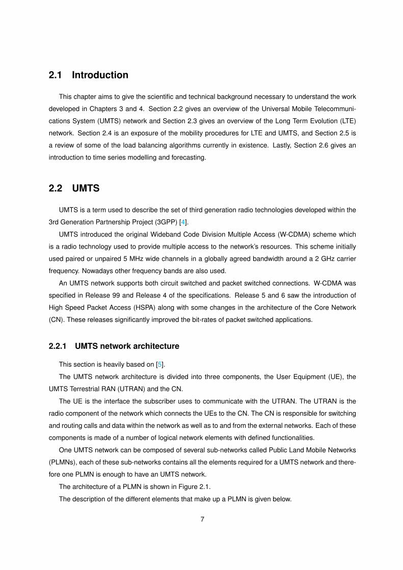
The architecture of a PLMN is shown in Figure 2.1.
The description of the different elements that make up a PLMN is given below.
7
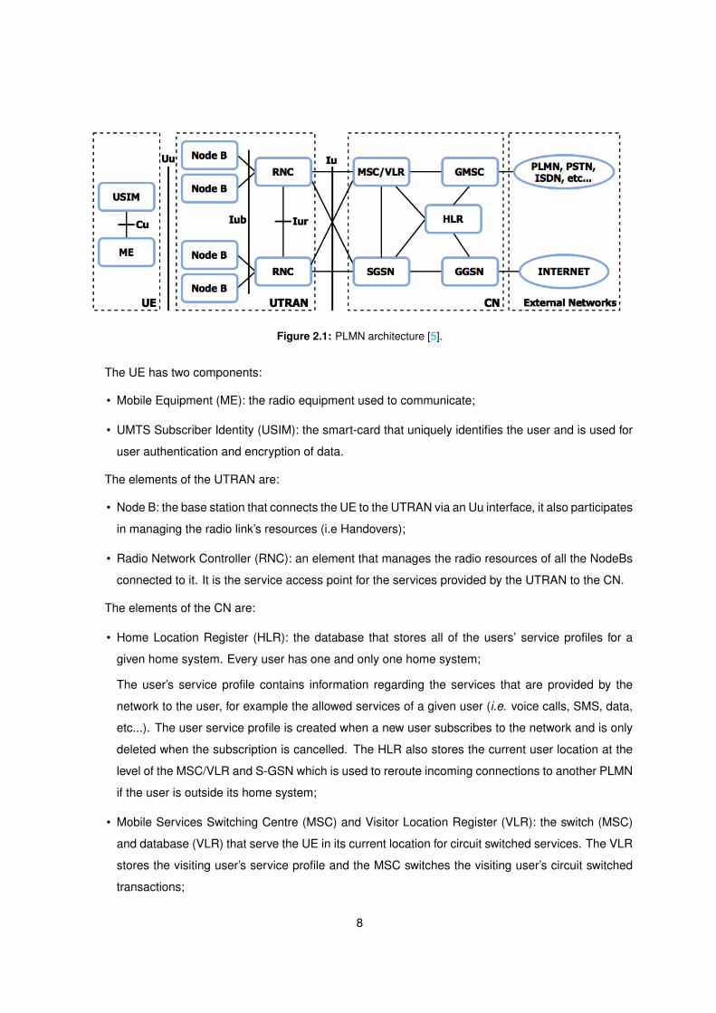
Figure 2.1: PLMN architecture [5].
The UE has two components:
• Mobile Equipment (ME): the radio equipment used to communicate;
• UMTS Subscriber Identity (USIM): the smart-card that uniquely identifies the user and is used for
user authentication and encryption of data.
The elements of the UTRAN are:
• Node B: the base station that connects the UE to the UTRAN via an Uu interface, it also participates
in managing the radio link’s resources (i.e Handovers);
• Radio Network Controller (RNC): an element that manages the radio resources of all the NodeBs
connected to it. It is the service access point for the services provided by the UTRAN to the CN.
The elements of the CN are:
• Home Location Register (HLR): the database that stores all of the users’ service profiles for a
given home system. Every user has one and only one home system;
The user’s service profile contains information regarding the services that are provided by the
network to the user, for example the allowed services of a given user (i.e. voice calls, SMS, data,
etc...). The user service profile is created when a new user subscribes to the network and is only
deleted when the subscription is cancelled. The HLR also stores the current user location at the
level of the MSC/VLR and S-GSN which is used to reroute incoming connections to another PLMN
if the user is outside its home system;
• Mobile Services Switching Centre (MSC) and Visitor Location Register (VLR): the switch (MSC)
and database (VLR) that serve the UE in its current location for circuit switched services. The VLR
stores the visiting user’s service profile and the MSC switches the visiting user’s circuit switched
transactions;
8

• Serving General Packet Radio Service (GPSR) Support Node (S-GW): similar to the MSC/VLR
but for packet switched services;
• Gateway MSC (G-MSC): the switch that connects the PLMN’s CN to the external circuit switched
networks;
• Gateway GPRS Support Node (G-GSN): is the point that connects the PLMN’s CN to external
packet switched networks.
The interfaces used to communicate between different network elements are:
• Cu interface: the electrical interface between the SIM card and the ME;
• Uu interface: the W-CDMA radio interface which allows the UE to access the fixed part of the
network;
• Iu interface: the interface that connects the UTRAN to the CN;
• Iur interface: the interface that allows for soft handovers between RNCs;
• Iub interface: the interface that connects the Node B to the RNC.
All these interfaces are open standards (accessible by all) in order to motivate competition between
different manufacturers.
The architecture here described is the UMTS architecture specified before Release 5. Release 5
saw the introduction of many changes to the CN, both in the circuit switched domain and in the packet
switched domain.
In the circuit switched domain, the MSC was divided into the MSC server and the Media Gateway
(MGW) and the G-MSC was divide into the the G-MSC server and the MGW. The new functions of these
network nodes are as follows:
• The MSC or G-MSC server take care of the control functionality as the MSC or G-MSC did before,
but the user data goes via the MGW. One MSC/G-MSC server can control multiple MGWs, this
allows for better scalability in the network since only the number of MGWs needs to be increased;
• The MGW performs the switching for the user data and network inter-working processing.
Release 5 also also contains the first phase of IP Multimedia Subsystem (IMS), which enables a
standardised approach to the provision IP-based services. In the packet switched domain, the S-GSN
and the G-GSN were slightly enhanced, in addition, to provide IP-based services, the IMS has the
following new elements:
• Media Resource Function (MRF), which controls media stream resources or can mix different
media streams:
9

• Call Session Control Function (CSCF), which acts as the first contact point to the terminal in the
IMS;
• MGW Control Function (MGWCF), which handles protocol conversations.
2.2.2 W-CDMA
This section is based on [6].
W-CDMA is the radio technology used in the UMTS air interface to provide multiple access to the
network, that is several users sharing the same radio resources.
The main idea behind W-CDMA is to share the same bandwidth but separate data streams using
spreading codes. Each data stream uses an unique spreading code which allows for its reception
without interference from other streams.
The main characteristics of W-CDMA are:
• W-CDMA is a wide-band Direct-Sequence Code Division Multiple Access (DS-CDMA) system,
which means user information is multiplied by quasi-random bits (called chips) derived from Code
Division Multiple Access (CDMA) spreading codes. This technology allows for bit rates up to
2 Mbps by using a variable spreading factor and multi-code connections;
• W-CDMA uses a chip rate of 3.84 Mcps which leads to carrier bandwidth of approximately 5 MHz.
This classifies W-CDMA as a wide-band system which have performance benefits such as in-
creased multi-path diversity;
• W-CDMA supports highly variable user data rates, the user data rate is kept constant in intervals of
10 ms frames and thus can only change from frame to frame. The control of data rates is typically
done by the network to achieve optimum throughput for packet data services;
• For full-duplex connections, W-CDMA supports two basic modes of operation:
– Frequency Division Multiplexing (FDD): consists in using separate carrier frequencies for the
uplink and downlink;
– Time Division Multiplexing (TDD): consists sharing the same carrier frequency for the uplink
and downlink, but using it at different times.
To better understand the concept of spreading and de-spreading lets look at an example, Figure 2.2
demonstrates the basic concept of spreading and de-spreading where the data is assumed to be a bit
sequence of rate R.
The spreading operation is performed by multiplying each data bit by a sequence of 8 code bits or
chips. This results in a spread data which now occupies 8 times the original bandwidth, therefore the
10
spread factor is 8. To de-spread the data, the spread sequence is multiplied by the same chip sequence
which was used to spread the data initially, provided that the sequences are synchronised the original
data sequence is obtained, as shown in Figure 2.2.
Figure 2.2: Spreading and despreading in DS-CDMA [6].
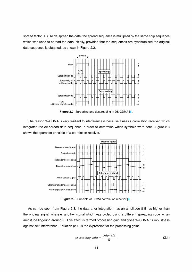
The reason W-CDMA is very resilient to interference is because it uses a correlation receiver, which
integrates the de-spread data sequence in order to determine which symbols were sent. Figure 2.3
shows the operation principle of a correlation receiver.
Figure 2.3: Principle of CDMA correlation receiver [6].
As can be seen from Figure 2.3, the data after integration has an amplitude 8 times higher than
the original signal whereas another signal which was coded using a different spreading code as an
amplitude lingering around 0. This effect is termed processing gain and gives W-CDMA its robustness
against self-interference. Equation (2.1) is the expression for the processing gain:
processing gain =chip rate
R, (2.1)
11

where the chip rate is 3.84 Mcps and R is the data rate. Note that the higher the data rate is, the lower
the processing gain will be. As an example, a speech service with rate 12.2 kbps will have a processing
gain of 25 dB. This mechanism allows for detection even if the signal power is low, in fact in some cases
the signal may even be below the thermal noise level making it hard to detect without the spreading code
and this is why this type of system originated in military applications.
The W-CDMA properties described above lead to the following consequences:
• The processing gain and wide-band nature of the system suggest a frequency reuse of 1 between
cells in a wireless system;
• Having many users sharing the same wide-band carrier provides interference diversity which will
average out the power of the interferers. This will boost system capacity when compared with
systems planned for worst case interference;
• The use of the previous two benefits requires tight power control and soft handovers to avoid users
blocking each others signals;
• Wide-band signals can resolve different propagation paths of a radio signal with higher accuracy
than signals with lower bandwidths. This results in more diversity against fading and thus improved
performance.
The spreading code is also known as channelisation code, channelisation codes are used for sepa-
rating physical data on the uplink, separating control channels form the same terminal on the uplink and
separating connections of different users within one cell in the downlink.
After the channelisation code, the data is multiplied by another code called scrambling code as shown
in Figure 2.4.
Figure 2.4: Relation between spreading and scrambling [6].
The scrambling code is used to separate terminals on the uplink and to separate cells on the down-
link.
12
2.3 LTE
LTE is a 4G wireless communication standard developed by 3GPP. It is the access part of the Evolved
Packet System (EPS) and it was created under the requirements of high spectral efficiency, high peak
data rates, short round trip time as well as flexibility in frequency and bandwidth [7].
LTE introduced Orthogonal Frequency Division Multiple Access (OFDMA) as the radio link technol-
ogy used to access the network. Unlike UMTS, LTE does not support circuit switched connections, it is
a fully packet switched system where every service provided is built on top of the Internet Protocol (IP).
2.3.1 LTE network architecture
This section is based on [8,9].
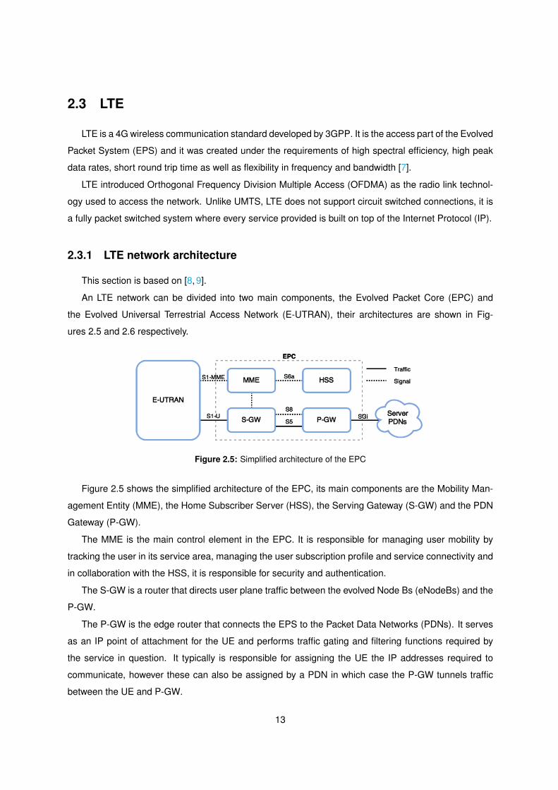
An LTE network can be divided into two main components, the Evolved Packet Core (EPC) and
the Evolved Universal Terrestrial Access Network (E-UTRAN), their architectures are shown in Fig-
ures 2.5 and 2.6 respectively.
Figure 2.5: Simplified architecture of the EPC
Figure 2.5 shows the simplified architecture of the EPC, its main components are the Mobility Man-
agement Entity (MME), the Home Subscriber Server (HSS), the Serving Gateway (S-GW) and the PDN
Gateway (P-GW).
The MME is the main control element in the EPC. It is responsible for managing user mobility by
tracking the user in its service area, managing the user subscription profile and service connectivity and
in collaboration with the HSS, it is responsible for security and authentication.
The S-GW is a router that directs user plane traffic between the evolved Node Bs (eNodeBs) and the
P-GW.
The P-GW is the edge router that connects the EPS to the Packet Data Networks (PDNs). It serves
as an IP point of attachment for the UE and performs traffic gating and filtering functions required by
the service in question. It typically is responsible for assigning the UE the IP addresses required to
communicate, however these can also be assigned by a PDN in which case the P-GW tunnels traffic
between the UE and P-GW.
13
The Policy and Charging Rules Function (PCRF) is connected to the P-GW, this element is respon-
sible for managing the user’s Quality of Service (QoS) and data charges, the information is provided to
the P-GW for enforcement.
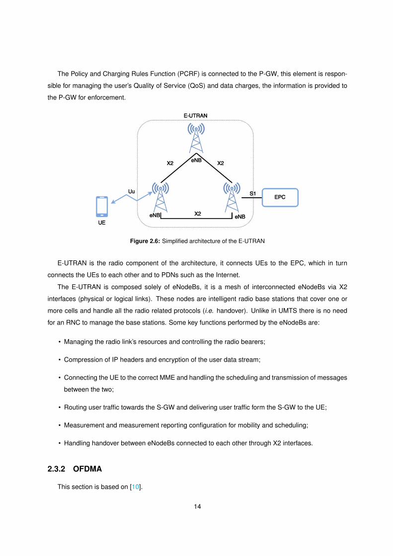
Figure 2.6: Simplified architecture of the E-UTRAN
E-UTRAN is the radio component of the architecture, it connects UEs to the EPC, which in turn
connects the UEs to each other and to PDNs such as the Internet.
The E-UTRAN is composed solely of eNodeBs, it is a mesh of interconnected eNodeBs via X2
interfaces (physical or logical links). These nodes are intelligent radio base stations that cover one or
more cells and handle all the radio related protocols (i.e. handover). Unlike in UMTS there is no need
for an RNC to manage the base stations. Some key functions performed by the eNodeBs are:
• Managing the radio link’s resources and controlling the radio bearers;
• Compression of IP headers and encryption of the user data stream;
• Connecting the UE to the correct MME and handling the scheduling and transmission of messages
between the two;
• Routing user traffic towards the S-GW and delivering user traffic form the S-GW to the UE;
• Measurement and measurement reporting configuration for mobility and scheduling;
• Handling handover between eNodeBs connected to each other through X2 interfaces.
2.3.2 OFDMA
This section is based on [10].
14
As discussed in Section 2.2.2, UMTS uses W-CDMA to provide multiple access. LTE introduced two
multiple access technologies, OFDMA is used for the downlink and Single Carrier Frequency Division
Multiple Access (SC-FDMA) is used for the uplink.
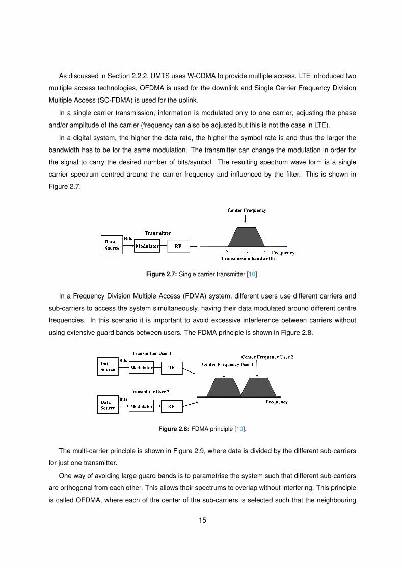
In a single carrier transmission, information is modulated only to one carrier, adjusting the phase
and/or amplitude of the carrier (frequency can also be adjusted but this is not the case in LTE).
In a digital system, the higher the data rate, the higher the symbol rate is and thus the larger the
bandwidth has to be for the same modulation. The transmitter can change the modulation in order for
the signal to carry the desired number of bits/symbol. The resulting spectrum wave form is a single
carrier spectrum centred around the carrier frequency and influenced by the filter. This is shown in
Figure 2.7.
Figure 2.7: Single carrier transmitter [10].
In a Frequency Division Multiple Access (FDMA) system, different users use different carriers and
sub-carriers to access the system simultaneously, having their data modulated around different centre
frequencies. In this scenario it is important to avoid excessive interference between carriers without
using extensive guard bands between users. The FDMA principle is shown in Figure 2.8.
Figure 2.8: FDMA principle [10].
The multi-carrier principle is shown in Figure 2.9, where data is divided by the different sub-carriers
for just one transmitter.
One way of avoiding large guard bands is to parametrise the system such that different sub-carriers
are orthogonal from each other. This allows their spectrums to overlap without interfering. This principle
is called OFDMA, where each of the center of the sub-carriers is selected such that the neighbouring
15
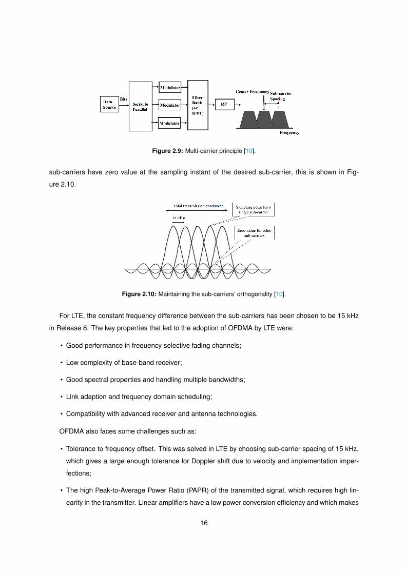
Figure 2.9: Multi-carrier principle [10].
sub-carriers have zero value at the sampling instant of the desired sub-carrier, this is shown in Fig-
ure 2.10.
Figure 2.10: Maintaining the sub-carriers’ orthogonality [10].
For LTE, the constant frequency difference between the sub-carriers has been chosen to be 15 kHz
in Release 8. The key properties that led to the adoption of OFDMA by LTE were:
• Good performance in frequency selective fading channels;
• Low complexity of base-band receiver;
• Good spectral properties and handling multiple bandwidths;
• Link adaption and frequency domain scheduling;
• Compatibility with advanced receiver and antenna technologies.
OFDMA also faces some challenges such as:
• Tolerance to frequency offset. This was solved in LTE by choosing sub-carrier spacing of 15 kHz,
which gives a large enough tolerance for Doppler shift due to velocity and implementation imper-
fections;
• The high Peak-to-Average Power Ratio (PAPR) of the transmitted signal, which requires high lin-
earity in the transmitter. Linear amplifiers have a low power conversion efficiency and which makes
16
them not ideal for mobile uplinks. In LTE this was solved by using the SC-FDMA for the uplink,
since this enables better power amplifier efficiency.
OFDMA is based on the Discrete Fourier Transform (DFT) and its inverse operation the Inverse
Discrete Fourier Transform (IDFT). These transformations allow moving the signal from the time domain
to the frequency domain and back again.
In practical applications the Fast Fourier Transform (FFT) and Inverse Fast Fourier Transform (IFFT)
are used. Provided that the sampling rate requirements of digital signal processing are met, these
operations can be carried out back and forth without loss of information.
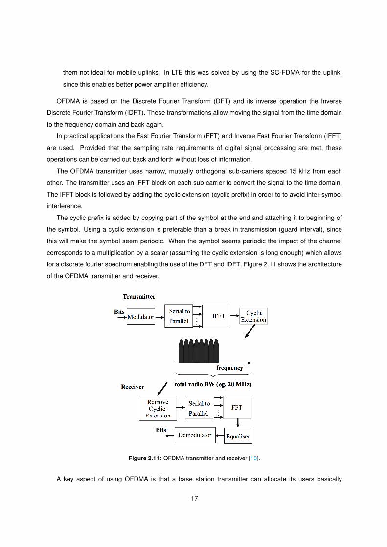
The OFDMA transmitter uses narrow, mutually orthogonal sub-carriers spaced 15 kHz from each
other. The transmitter uses an IFFT block on each sub-carrier to convert the signal to the time domain.
The IFFT block is followed by adding the cyclic extension (cyclic prefix) in order to to avoid inter-symbol
interference.
The cyclic prefix is added by copying part of the symbol at the end and attaching it to beginning of
the symbol. Using a cyclic extension is preferable than a break in transmission (guard interval), since
this will make the symbol seem periodic. When the symbol seems periodic the impact of the channel
corresponds to a multiplication by a scalar (assuming the cyclic extension is long enough) which allows
for a discrete fourier spectrum enabling the use of the DFT and IDFT. Figure 2.11 shows the architecture
of the OFDMA transmitter and receiver.
Figure 2.11: OFDMA transmitter and receiver [10].
A key aspect of using OFDMA is that a base station transmitter can allocate its users basically
17
any sub-carrier in the frequency domain. The possibility of having different sub-carriers allocated to
users enables the scheduler to benefit from frequency diversity. Due to overhead caused by signalling
resolution, in LTE allocation is not done on an individual sub-carrier level basis but is based on Physical
Resource Blocks (PRBs), each one consisting of 180 kHz. The respective allocation resolution in the
time domain is 1 ms also denoted by one Transmission Time Interval (TTI), however, each PRB lasts
only 0.5 ms. Each PRB can be modulated independently, LTE uses Quadrature Amplitude Modulation
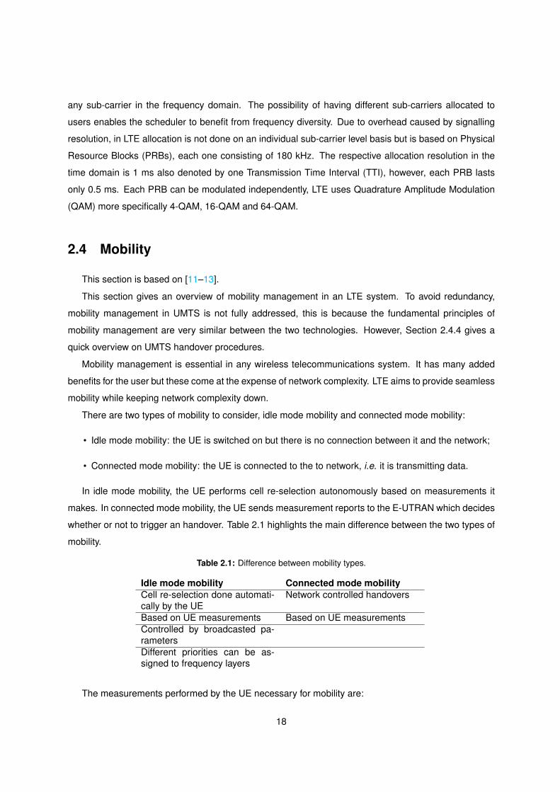
(QAM) more specifically 4-QAM, 16-QAM and 64-QAM.
2.4 Mobility
This section is based on [11–13].
This section gives an overview of mobility management in an LTE system. To avoid redundancy,
mobility management in UMTS is not fully addressed, this is because the fundamental principles of
mobility management are very similar between the two technologies. However, Section 2.4.4 gives a
quick overview on UMTS handover procedures.
Mobility management is essential in any wireless telecommunications system. It has many added
benefits for the user but these come at the expense of network complexity. LTE aims to provide seamless
mobility while keeping network complexity down.
There are two types of mobility to consider, idle mode mobility and connected mode mobility:
• Idle mode mobility: the UE is switched on but there is no connection between it and the network;
• Connected mode mobility: the UE is connected to the to network, i.e. it is transmitting data.
In idle mode mobility, the UE performs cell re-selection autonomously based on measurements it
makes. In connected mode mobility, the UE sends measurement reports to the E-UTRAN which decides
whether or not to trigger an handover. Table 2.1 highlights the main difference between the two types of
mobility.
Table 2.1: Difference between mobility types.
Idle mode mobility Connected mode mobilityCell re-selection done automati-cally by the UE
Network controlled handovers
Based on UE measurements Based on UE measurementsControlled by broadcasted pa-rametersDifferent priorities can be as-signed to frequency layers
The measurements performed by the UE necessary for mobility are:
18
• Reference Signal Received Power (RSRP): the average power measured in a cell (across receiver
branches) of the resource elements that contain cell-specific reference signals;
• Reference Signal Received Quality (RSRQ): the ratio of the RSRP and the E-UTRA Carrier Re-
ceived Signal Strength Indicator (RSSI), for the reference signals.
• RSSI: the total received wide-band power on a given frequency. It includes the noise from interfer-
ing cells and other noise sources. RSSI is not reported by the UE as an individual measurement,
but it is only used in calculating the RSRQ value inside the UE.
For inter-system mobility between LTE and UMTS the following measures are necessary:
• UTRA FDD Common Pilot Channel (CPICH)’s Received Signal Code Power (RSCP): represents
the power measured on the code channel used to spread the primary pilot channel on W-CDMA;
• UTRA FDD (and TDD) carrier’s RSSI: represents the corresponding wide-band power measure-
ment as also defined for LTE;
• UTRA FDD CPICH’s Ec/No: represents the quality measurement, like RSRQ in LTE, and provides
the received energy per chip energy over the noise;
• UTRA TDD Primary Common Control Physical Channel (P-CCPCH)’s RSCP: represents the code
power of the UTRA TDD broadcast channel.
2.4.1 Idle mode mobility
In idle mode mobility the UE selects a cell based on radio measurements. This procedure is called
cell selection, when a UE selects a cell it is said that the UE camped in that cell. For the UE to camp
in a cell it is required good radio quality and that the cell is not blacklisted. For a cell to be a suitable
candidate it has to fulfil the S-criterion:
Srxlevel > 0 , (2.2)
where
Srxlevel > Qrxlevelmeas − (Qrxlevmin −Qrxlevelminoffset) , (2.3)
and Srxlevel is the cell selection Rx level value, Qrxlevelmeas is the measured cell received level
(RSRP), Qrxlevmin is the minimum required received level in dBm and Qrxlevelminoffset is an offset used
when searching for a higher priority PLMN1.
1LTE allows setting priority levels for PLMNs in order to specify preferred network operators in cases such as roaming.
19
After the UE has camped on a cell it may continue to find better cells for re-selection according to the
re-selection criteria. Intra-frequency and equal priority intra-E-UTRAN inter-frequency cell re-selection
are based on the cell ranking criterion, also known as the R-criterion. The UE must measure the
neighbouring cells, which are indicated in the neighbour list of the serving cell, and choose the best
candidate from the list.
The network may prevent the UE from considering some cells for re-selection by blacklisting them.
To limit the number of re-selections measurements made, it has been defined that if the serving cell’s
Rx level value, SServingCell, is high enough the UE does not need to make any intra-frequency, inter-
frequency or inter-system measurements. The measurements resume once SServingCell ≤ Sintrasearch
for intra-frequency measurements, and SServingCell ≤ Snonintrasearch for inter-frequency measurements.
The serving cell ranking is defined as Rs :
Rs = Qmeas,s +Qhyst , (2.4)
and a neighbouring cell’s ranking as Rn:
Rn = Qmeas,n +Qoffset , (2.5)
whereQmeas is the RSRP measurement, Qhyst is the power domain hysteresis to avoid ping-ponging be-
tween cells and Qoffset is control parameter to account for different frequency and/or cell characteristics
such as propagation properties. The re-selection occurs to the best ranked neighbour cell if it is ranked
better than the serving cell for longer than a time Tre−selection, this limits overly frequent re-selections.
The Qhyst provides hysteresis meaning that the neighbour cell must be better than the serving cell by a
configurable amount for re-selection to occur, and the Qoffset allows for bias in the re-selection process.
In LTE, inter-frequency (different priorities) and inter-system re-selection are based on method called
layers which allows the operators to control how the UE prioritises camping on different Radio Access
Technologies or frequencies. The method is known as absolute priority based re-selection, each layer
is assigned a priority and the UE tries to camp on the highest priority layer than can provide decent
service. A UE will camp on a higher priority layer if the layer is above a threshold Treshhigh for longer
than a re-selection period Tre−selection. The UE will only camp to a lower priority layer if the higher layer
drops below the threshold Treshhigh and the lower layer rises above the threshold Treshlow.
It is common to pass the measurements through a low-pass filter in order to average them over time.
This shields the measurement process from fast fading effects, preventing unnecessary cell re-selections
or the none occurrence of a necessary cell re-selections.
20
2.4.2 Handover
In LTE handovers are based in measurements made by the UE but controlled by the E-UTRAN.
LTE uses only hard handovers which are targeted to be lossless by using packet forwarding between
the source and target eNodeBs. The path the traffic makes through the core network is only updated
after the handover is done, this called late path switching. Before sending a measurement report to the
eNodeB, an UE must identify and measure the target cell. After receiving the measurement report, the
E-UTRAN may decide or not to trigger the handover.
LTE supports inter-Radio Access Technology (RAT) handovers which are inter-system handovers
between the E-UTRAN and GSM EDGE Radio Access Network (GERAN), UTRAN or cdma2000®.
The inter-RAT handover is controlled by the source access system, which makes the measurements
and the handover execution decision. The inter-RAT handover is a backwards handover meaning that
the radio resources are reserved in the target system before the handover command is issued to the
UE2. All the signalling is done through the core network since there are no interfaces between the
different radio access systems. All the information regarding the target system is given to the UE by the
source system and the user data can be forwarded from the source system to the target system to avoid
the loss of data.
As is in idle mobility, the handover decision is based on measurements of the RSRP or RSRQ, the
UE will request an handover if the signal of the serving cell plus an handover margin drops below the
signal of a neighbouring cell [14, 15]. The handover margin is an offset plus an hysteresis value which
are used to avoid unnecessary handovers and also the ping-pong effect.
In LTE, handovers are triggered by event A3 for intra-LTE handovers and by event B2 for inter-RAT
handovers [14,15].
• The A3 event is triggered when the signal of neighbouring LTE cell becomes higher than the signal
of the serving cell plus the handover margin. The entering condition for the A3 event is:
Mn+Ofn+Ocn−Hys > Ms+Ofs+Ocs+Off , (2.6)
where Mn is the measurement of the neighbouring cell, Ms is the measurement of the serving
cell, Ofn and Ofs are the frequency specific offsets of the neighbouring and serving cells, Ocn
and Ocs are the cell specific offsets of the neighbouring and serving cells, Off is the tunable offset
parameter and Hys is the hysteresis parameter. Mn and Ms are measured in dBW or dBm and
all the other quantities are measured in dB.
2With the exception of GERAN which does not support packet switched handovers.
21

The leaving conditions for event A3 is:
Mn+Ofn+Ocn+Hys < Ms+Ofs+Ocs+Off . (2.7)
• The B2 event is triggered when the the signal from the serving cell drops below a threshold and
the signal from a inter-system cell rises above another threshold. The entering condition for event
B2 is:
Ms+Hys < Thresh1∧
Mn+Ofn+Ocn−Hys > Thresh2 , (2.8)
and the leaving condition is:
Ms−Hys > Thresh1∨
Mn+Ofn+Ocn+Hys < Thresh2 . (2.9)
In both cases, the handover event is only triggered if the entering condition remains true for longer
than a time to trigger, Ttrigger, to avoid unnecessary handovers and the ping-pong effect.
In order to mitigate the effects that fast fading has on the measurements, the measurements are
passed through a filter that averages the measurements over time. This filter helps to prevent unneces-
sary handovers and is described in Section 2.4.3.
In order to save power, the UE does not need to measure the neighbouring cells at all times, it is
possible to set thresholds that trigger the start and end of the measuring process. These events are
called A1 and A2 and are defined as:
• A1: Signal from the target cell becomes better than threshold;
• A2: Signal from the serving cell becomes worse than threshold.
Figure 2.12 shows an handover procedure, where it is possible to see the aforementioned handover
events as function of the source and target cells’ RSRP.
Some typical values for the handover parameters can be found in [15] where Ericsson recommends
the following parameters, regarding intra-LTE handover parameters:
• The trigger quantity should be the measured RSRP of the serving and neighbouring cells;
• The hysteresis parameter should be 4 dB;
• The time to trigger, Ttrigger, should be 40 ms;
• The offset should be 0 dB;
• For higher loads the hysteresis should be 1 dB and the offset 3 dB.
22
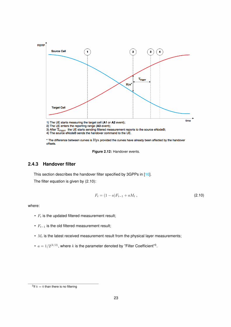
Figure 2.12: Handover events.
2.4.3 Handover filter
This section describes the handover filter specified by 3GPPs in [16].
The filter equation is given by (2.10):
Ft = (1− a)Ft−1 + aMt , (2.10)
where:
• Ft is the updated filtered measurement result;
• Ft−1 is the old filtered measurement result;
• Mt is the latest received measurement result from the physical layer measurements;
• a = 1/2(k/2), where k is the parameter denoted by ”Filter Coefficient”3.
3If k = 0 than there is no filtering
23
2.4.4 The handover in UMTS (3G)
This section is based on [6,17].
In UMTS, handovers are controlled by the RNC which decides when and to where the handover is
made. Nonetheless, the handover is based on UE measurements of the Signal to Interference Ratio
(SIR) (Ec/I0) of the CPICH from different eNodeBs.
For intra-system intra-frequency handovers, UTMS uses soft and softer handovers, during which the
UE communicates concurrently via two air interfaces. For inter-frequency and inter-system handovers,
UMTS use hard handovers, during which the UE is not communicating via any air interface. As a result,
the handover delay must be small.
The following terminology applies in UMTS handovers:
• Active set: The set of cells that form a soft handover connection with the UE;
• Neighbouring set: The set of cells which are being monitored by the UE but whose pilot Ec/I0 is
not strong enough to be added to the active set.
There are three events related to soft and softer handovers:
• 1A or Radio Link Addition: add a cell to the active set;
• 1B or Radio Link Removal: remove a cell from the active set;
• 1C or Combined Radio Link Addition and Removal: when the active set is full the weakest cell in
the active set is removed.
In the UTRAN, inter-frequency and inter-RAT re-selections are based on the same ranking as intra-
frequency re-selections. This proved difficult for the network to control as the measurement quantities
of different RATs are different and the network needs to be able to control re-selection between multiple
3GPPs RATs (or even non-3GPPs technologies).
2.5 Load balancing review
This section is based on [18] as well as the sources cited in the text.
The process of balancing network load between neighbouring cells in space, frequency or system is
called load balancing. During periods of high network resource utilisation some cells might become over-
loaded while its neighbours still have resources not being used. Overloaded cells can cause declines in
the QoS provided due to lack of resources and deteriorate the overall network performance. This prob-
lem is caused by an inefficient utilisation of the total available network resources and can be mitigated by
using load balancing techniques. Load balancing is performed by triggering the mobility mechanisms of
24

a RAT resulting in the transit of UEs to neighbouring cells. The neighbouring cells can be intra-frequency
intra-RAT neighbours, inter-frequency intra-RAT neighbours or even inter-RAT neighbours.
To perform load balancing it is first necessary to have a measure of the cell’s load. The load of a
cell can be measured directly by looking at the resource utilisation of a cell or indirectly by looking at
measures that can indicate problems in a cell. Direct measures of a cell’s load include:
• The number of allocated PRBs in LTE;
• The number of Channel Elements (CEs) used in UMTS.
Some indirect measures of a cell’s load are:
• The downlink/uplink throughput;
• The number of unsatisfied users;
• The total transmitted and received power;
• The Signal to Interference plus Noise Ratio (SINR);
• Blocking probability of new active users.
Load balancing techniques can be applied to idle mode users or connected mode users. Load
balancing for connected users its easier to perform because the network has measures of the user’s
radio conditions and traffic requirements before deciding whether to perform load balancing. Idle mode
load balancing is more difficult because the network does not know in advance what radio conditions
the user will have and what resources the user will require.
The classical mechanism to perform load balancing in LTE is to adjust the cell’s effective coverage
area in order to trigger the UE to make a cell re-selection or handover, this can be done by remotely
controlling the electrical tilt and transmitted power of the antennas, or by adjusting the cell re-selection
and handover parameters.
This first mechanism is somewhat impractical due to having to make actual physical changes in the
network. On the other hand, the second mechanism is able to artificially change the effective coverage
area of a cell without impacting the actual received signal power and making physical changes to the
network. Since the first mechanism directly impacts the signal power, it can cause coverage holes due
to the coverage area of the cell being highly non-uniform in reality. Nonetheless, the first mechanism is
not as susceptible to interference as the second.
Since changing the cell re-selection and handover parameters is easier most of the research is
focused on this solution. These parameters can be optimised in an open loop, i.e. the parameters are
optimised once and implemented in the network, or in a closed loop.
25
A network which optimises parameters in a closed loop is called a SON. SONs are networks capable
of actively and autonomously controlling the networks parameters, based on real time measurements.
These type of networks work in real time in order to adapt and adjust to a changing situation.
In [19] 3GPP standardises the measurements, procedures and open interfaces to support better
inter-operability in a multi-vendor environment for SONs. In this standard 3GPPs introduces the frame-
work for two mobility SON algorithms called Mobility Robustness Optimisation (MRO) and Mobility Load
Balancing (MLB). These frameworks do not directly specify the algorithm to be used, instead they specify
the objectives, inputs, outputs and expected results of the algorithm.
2.5.1 Mobility Robustness Optimisation
This section is based on [19].
In 2G/3G systems handover parameters were set manually and were costly to update after initial
deployment, to address this issue MRO proposes the detection and automatic fix of mobility problems.
The main objective of the algorithm is to reduce handover related Radio Link Failures (RLFs) and the
secondary objective is the reduction of the inefficient use of network resources due to unnecessary or
missed handovers [19]. Handover failures can be due to:
• Too Late Handovers (TLH);
• Too Early Handovers (TEH);
• Handover to the Wrong Cell (HWC).
Inefficient network resource usage may result from non-optimal configuration of handover parameters
even if it does not result in RLFs, for example, incorrectly setting the handover hysteresis may be the
reason for either the ping-pong effect or prolonged connection to non-optimal cell [19].
MRO should be able to detect TLH, TEH and HWC with help of RLF reports from neighbouring cells.
The algorithm should be able to minimise the number of failed or unnecessary handovers by optimising
the following parameters:
• Hysteresis;
• Time to Trigger;
• Cell Individual Offset;
• Cell re-selection parameters.
26
2.5.1.A An inter-RAT MRO implementation
In [20] the authors propose a SON-based algorithm for optimising inter-RAT handover thresholds.
The algorithm runs on both LTE and 3G networks and uses inter-RAT Key Performance Indicators
(KPIs) that capture the number and type of mobility failure events4to feed a proportional feedback con-
troller which controls the handover thresholds [20].
The simulation results showed that the proposed algorithm outperformed three distinct network-wide
settings of handover thresholds in reducing the number of RLFs, and implied the importance of cell-
specific handover thresholds depending on the mobility and traffic conditions in different handover areas
[20].
The algorithm was also shown to converge faster and perform better than the Taguchi’s method
[21,22] which is statistical optimisation algorithm recently also applied to engineering.
2.5.2 Mobility Load Balancing
The objective of MLB is to optimise cell re-selection/handover parameters in order to cope with the
unequal traffic load, and to minimise the number of handovers and re-directions needed to achieve the
load balancing [19].
“Self-optimisation of the intra-LTE and inter-RAT mobility parameters to the current load in the cell
and in the adjacent cells can improve the system capacity compared to static/non-optimised cell re-
selection/handover parameters” [19].
The optimisation should minimise human intervention in network management and optimisation tasks
and not compromise the QoS provided when compared to the case with normal mobility without load
balancing.
Load balancing can be done in two scenarios:
• Intra-LTE load balancing;
• Inter-RAT load balancing.
The specification states that an eNodeB should monitor its controlled cells and exchange load related
information via an X2 or S1 interface with its neighbours, after, an algorithm should distribute the load
towards adjacent or co-located cells including cells from other RATs.
After the algorithm is used, it is expected that the load is balanced, the capacity of the system
increases and human intervention is minimised.
4Such as the number of too late handovers, too early handovers, unnecessary handovers, ping-pong scenarios and handoversto the wrong cell.
27
For intra-LTE load balancing the algorithm should optimise the handover parameters changing the
handover trigger threshold, for inter-RAT load balancing [19] does not specify which parameters should
be optimised.
It is important to note that MRO and MLB may conflict when the objective of reducing the amount of
failed and unnecessary handovers clashes with the objective of balancing the load. This happens when
both algorithms try to move the same parameter in opposite directions or even to different values in the
same direction.
The following sections aim to provide a brief literature review of the different types of load balancing
methods already in existence.
2.5.2.A MLB Implementations
In [23] a load balancing algorithm for idle mode mobility is proposed. The algorithm adjusts cell
re-selection parameters instead of handover parameters. This is done in order for the load balancing
algorithm not to interfere with MRO algorithms that may be changing the handover parameters. The
authors show that the algorithm reaches considerable throughput gains for the simulated scenarios.
In [24] the authors propose a load balancing algorithm for a SON which uses virtual load measures
to try to minimise the number of unsatisfied users in the network. The paper uses a simulation scenario
where a bus route creates load imbalances in the network. The authors go on to show that algorithm
manages to have less unsatisfied users in the simulation scenario when the algorithm is active then in
the reference scenario where the algorithm was not used.
In [25] the authors propose a game theory approach to load balancing. The network is divided into
zones and uses a Cournot game model to balance the load. The Cournot game model can be used
to describe commodity exchange process among a limited number of monopoly companies involving
several parameters of price and production of a specific commodity [25]. By regarding traffic load bearing
of a cell as the commodity, the load balancing algorithm achieves optimal values for the parameters that
mediate interactions between the cells [25]. The simulation results showed that the proposed algorithm
overcomes the ping-pong and slow-convergence problems of more conventional approaches to MLB.
In [26] the authors propose a load balancing algorithm that is formulated as an optimisation prob-
lem. The algorithm uses the SINR and bandwidth efficiency of the network to construct an optimisation
variable. The goal is then to find which network parameters minimise the optimisation problem. The
simulation results showed that the proposed algorithm can efficiently decrease the new call blocking
rate, reduce network resources occupation and increase the network bandwidth efficiency [26].
In [27] the authors use a neuro-fuzzy inference system to tackle the load balancing problem This
approach uses a soft computing concept called fuzzy logic, which denotes probabilities of a state instead
of true or false, combined with a machine learning concept denoted neural network to form what is
28
called an adaptive neuro-fuzzy inference system. In [27] the authors introduce three key performance
indicators, the number of satisfied (dissatisfied) users, the fairness index and the virtual load of the
source and show that the developed algorithm is able to sustain a load balancing process by decreasing
the hysteresis value when the number of unsatisfied users increases. There are no simulation results
presented in [27]. In [28], the authors present another algorithm based on fuzzy logic and shows that it
can be balance bandwidth utilisation and reduce blocking probability when compared with a case where
no load balancing is made. Neither [27] or [28] present a comparison between their methods and simpler
load balancing approaches.
2.6 Forecasting
Predicting the evolution of network traffic over time can be extremely helpful in mid to long term
system capacity planning.
Given a set of traffic observations spread across time in equally distant intervals (e.g. daily observa-
tions), it is possible to try to predict the evolution of traffic in the future based on its previous behaviour.
The sequence of traffic observations can be seen as a time series, “a time series is a set of observations
xt, each one being recorded at a specific time t” [29].
Since the behaviour of network traffic in the future is inherently uncertain, meaning the behaviour of
the time series is not fully deterministic, each observation xt can be seen as a realisation of a random
variable Xt. In other words, the observed time series xt is a realisation of a sequence of random
variables Xt [29].
If a probabilistic model describing Xt can be determined, then it is possible to forecast, with a level
of confidence, the value of future observations of xt, using said model. The definition of probabilistic
model of a time series can be found in Appendix A.
The process of fitting a probabilistic model to describe Xt given a set of observations xt is called
time series modelling or model fitting. A model can also be seen as a function that outputs the next
value in the time series (forecast) given the previous ones (observations).
To fit a model to a time series it is necessary to understand some basic concepts regarding time
series. The concepts of mean, Autocorrelation Function (ACF), Partial Autocorrelation Function (PACF)
and wide sense stationarity are defined in Appendix A.
Once the model is fitted it can be used to forecast future observations, this is done by using the
model’s formula to obtain the next observation in the series. To get a larger forecasting horizon5the
model is applied recursively taking each forecast as an observation to be used in the next iteration.
Another method of forecasting is to do a rolling forecast, this means that instead of taking the fore-
5The forecasting horizon is the number of observations in the future that are being predicted.
29

casted value as an observation, one waits until the actual observation is available to use for the next
forecast. This method only allows for one forecast at a time but it has the benefit of added accuracy
since the forecasting horizon is always one observation. It is possible to refit the model at any time to
account for changes in the time series behaviour, depending on the data one may choose to refit the
model every any fixed amount of observations (e.g. refit the model every week for daily observations).
Since the modelled series Xt is a sequence of random variables it is possible to forecast not only
its mean but also its standard deviation, this allows us to obtain confidence intervals for the forecasted
mean. This intervals are called prediction intervals and are regions where the forecast is expected to be
in, with a given probability. Commonly used prediction intervals include the 80% and 95% confidence
intervals [30]. Prediction intervals tend to increase in size as the forecasting horizon increases [30],
this is due to the recursive manner in which forecasting is made which propagates error forward leading
to higher uncertainty. As a result, choosing a reasonable forecasting horizon is important, since the
forecasts’ validity decrease as the forecasting horizon increases.
2.6.1 Diagnostics
After fitting a model to a time series it is important to determine whether the model is a good fit for
the data. This section presents several complementary techniques for model selection and diagnostics.
2.6.1.A The Akaike Information Criterion
The Akaike Information Criterion (AIC) [31] is a measure used to compare the quality of different
statistical models fitted to the same data. It measures the amount of information lost after fitting the
model. It can measure the relative quality of one model in comparison with others, it does not give an
absolute verdict on fit’s quality. The AICc [30, 32] is the AIC adjusted to penalise more complex models
and avoid overfitting. To choose between models using the AICc, the model with the lowest AICc is
chosen, i.e. the one which lost the least amount of information.
2.6.1.B Forecasting errors
The most intuitive tool for diagnostics are error metrics, these metrics measure the discrepancy
between the forecast and the observation.
The simplest error metrics are scale-dependent errors, these errors can only be used to compare
accuracy of different fits on the same time series, because their values depend directly on the values of
the observations.
The forecast error is defined as
ei = yi − yi , (2.11)
30
where yi is the observation and yi is the forecast.
The Mean Absolute Error (MAE) is
MAE = mean(|ei|) , (2.12)
and the Root Mean Square Error (RMSE) is
RMSE =√mean(e2i ) . (2.13)
Percentage errors are more useful than scale-dependent errors because they allow the comparison
between different models on different time series. In addition, with percentage errors it is easy to see in
relative terms how far from the observation the forecast is.
The percentage error is defined as:
pi =100eiyi
. (2.14)
The Mean Absolute Percentage Error (MAPE) is:
MAPE = mean(|pi|) . (2.15)
Scale-dependent and percentage errors can be problematic when the value of the observations is
0 or close to 0, this will trigger a division by 0 which will impede the calculation of the error metrics.
Because of this Rob J. Hyndman in [33] proposed the introduction of scaled errors.These errors are a
comparison between the naıve6forecast and the forecast performed by the model being tested, they can
be used to compare forecast accuracy across series on different scales without the problem of dividing
by 0.
The scaled error is defined as
qj =ej
1T−1
∑Tt=2 |yt − yt−1|
, (2.16)
where T is the length of the series.
The Mean Absolute Scaled Error (MASE) is
MASE = mean(|qj |). (2.17)
6The nıve forecast is simply taking the value of the last observation as the forecast.
31
2.6.1.C Training, validation and test sets
A common approach for model diagnostics widely used in the field of machine learning is to divide
the data into to three separate sets [34]. The training set is the one used to fit the model to the data. The
validation set is used to measure the accuracy of the fit (error metrics) and adjust the model’s parameters
accordingly. The test set is used in the end stage to determine the accuracy of the final model in a real
scenario.
There are several “rules of thumb” on how to split the data into training, validation, test sets, these
rules are not laws and the most adequate data split will depend on the situation.
In the case of time series modelling, the model is often adjusted using only the training set, in this
case no validation set is required.
Another machine learning technique is to use learning curves to determine if the model presents
high bias (overfitting) or high variance (underfitting) [34]. This is useful to determine whether more
observations are necessary.
2.6.1.D Residual diagnostics
The residuals of a fit are the difference between the observations and their forecasts (as in equa-
tion (2.11)). The residuals of a good fit will have the following properties [30]:
• “The residuals are uncorrelated. If there are correlations between residuals, then there is informa-
tion left in the residuals which should be used in computing forecasts” [30].
• “The residuals have zero mean. If the residuals have a mean other than zero, then the forecasts
are biased” [30].
In addition to these properties, it is useful for the residuals to have constant variance and be normally
distributed. These properties facilitate the calculation of prediction intervals.
2.6.2 Simple forecasting methods
Some of the more simple forecasting techniques methods include the average method, naıve method
and seasonal naıve method [30]. This methods have low complexity and therefore their forecasts are
extremely useful to use as benchmarks for more complex methods.
The average method is simply taking the mean of the time series as the forecast for the next ob-
servation [30]. The naıve method is to take the last observation and use it as the forecast for the next
observation [30]. In the seasonal naıve method a seasonal period m is defined and instead of using the
last observation as the forecast, the previous observation from the same season is used as the forecast
(the observation m observations before) [30].
32
2.6.3 ARMA family models
This section is based on [35–37], however, some of the formulas had to be deduced from the material.
There is a large family of models that fall under the category of Auto-Regressive Moving Average
(ARMA) models. These models are based on the assumption that the time series is a process whose
current value depends on its previous values.
A Moving Average (MA) process of lag q is a process whose current value depends on current and
past observations of a White Noise (WN) process up to a lag q. This process is written as MA(q). The
definition of a White Noise process is given in Appendix A.
Definition 2.6.1. “The MA(q) Process: Xt is a moving-average process of order q if:
Xt = Zt + θ1Zt−1 + . . .+ θqZt−q , (2.18)
where Zt ∼WN(0, σ2) and θ1, . . . , θq are constants” [35].
Proposition 2.6.1. The autocorrelation of an MA(q) process is zero for lags greater than q, this means
that if Xt is a stationary q-correlated time series it can be represented by an MA(q) process [35].
An Auto-Regressive (AR) process of lag p is a process whose current value depends on observations
of its past values up to a lag p, as well as a WN term. This process is written as AR(p)
Definition 2.6.2. “The AR(p) Process: Xt is a autoregressive process of order p if:
Xt =
p∑i=1
φiXt−i + Zt , (2.19)
where Zt ∼WN(0, σ2) and φ1, . . . , φp are constants” [35].
Proposition 2.6.2. The partial auto-correlation of an AR(p) process is zero for lags greater than p, this
means that if Xt is a stationary p-partially-correlated time series it can be represented by an AR(p)
process [35].
The combination of an AR(p) process with an MA(q) process is an ARMA(p, q) process called an
Auto-Regressive Moving Average process.
Definition 2.6.3. “Xt is an ARMA(p, q) process if Xt is stationary and if for every t,
Xt − φ1Xt−1 − · · · − φpXt−p = Zt + θ1Zt−1 + · · ·+ θqZt−q , (2.20)
33
where Zt ∼WN(0, σ2) and the polynomials (1−φ1z− . . .−φpzp) and (1 + θ1z+ . . .+ θqzq) have
no common factors” [36].
Alternatively, an ARMA process can be written as:
Xt = Zt +
p∑i=1
φiXt−i +
q∑i=1
θiZt−i , (2.21)
or
(1 +
p∑i=1
φiBi
)Xt =
(1 +
q∑i=1
θiBi
)Zt , (2.22)
where B is the lag operator, meaning that BiXt = Xt−i.
ARMA processes are extremely useful for describing stationary time series, however they do not
usually fit non-stationary time series. In order to use these models with non-stationary time series it is
first necessary to transform the series into a stationary time series. One of the transforms that is able to
accomplish this is differencing.
Suppose Yt is Xt d times differenced then:
Yt = (1−B)dXt. (2.23)
As an example, differencing Xt one time results in Xt −Xt−1.
The Auto-Regressive Integrated Moving Average (ARIMA) model is an expansion of the ARMA model
which can be used to fit non-stationary time series. These models are written as ARIMA(p, d, q):
(1 +
p∑i=1
φiBi
)(1−B)dXt = δ +
(1 +
q∑i=1
θiBi
)Zt, (2.24)
where p and q are the AR and MA terms, and d is the degree of differencing the series suffers before the
ARMA(p, q) model is fitted.
It is often the case that the time series shows strong seasonal behaviour, this means that its value
is similar every m observations, e.g. network traffic is higher in a business cell during the week than on
the weekend.
To allow for seasonality in the data, ARIMA models can be expanded by introducing a seasonal
component on top of an existing model, the seasonal component is simply another ARIMA model which
only works over intervals that are multiples of the seasonal period m.
These models are called Seasonal ARIMA (S-ARIMA) and are written asARIMA(p, d, q)×(P,D,Q)m:
(1 +
p∑i=1
φiBi +
P∑i=1
ΦiBm×i
)(1−B)d(1−Bm)DXt = δ +
(1 +
q∑i=1
θiBi +
Q∑i=1
ΘiBm×i
)Zt. (2.25)
34
In the network traffic example given previously, the seasonal period is m = 7 and the seasons are
the days of the week.
It is also possible to add to the model external regressors, this means to incorporate in the model
one or more time series with the same length as the time series to which the model will be fitted. The
external regressors can improve the fit by adding relevant information to the model, e.g. if a time series
has strong weekly seasonality, holidays during the week will probably present weekend-like behaviour
instead of week-like behaviour, in this case using an external regressor to denote whether a day is an
holiday or not might improve the fit.
2.6.3.A Fitting ARIMA models
To fit an ARIMA(p, d, q) × (P,D,Q)m model to the time series it is necessary do determine which
model parameters (p, d, q, P,D,Q) to use before estimating the model’s coefficients (φ1, . . . , φp and
θ1, . . . , θq). The most common approach to determine the model’s parameters is the Box-Jenkins
methodology introduced by G. Box and G. Jenkins in 1970 [38].
The first step in the Box-Jenkins method is to determine whether the time series is stationary and if
there exists any significant seasonality in the data. If seasonality is found to exist and the series is non-
stationary, it is important to determine whether the series is non-stationary in the seasonal component,
the non-seasonal component or both.
It is possible to detect seasonality by looking at the ACF plot, if this plot shows periodic spikes in
intervals ofm lags, then there is seasonality in the series of periodm. It is often the case that seasonality
is already known to exist in the data, as well as its period.
After identifying seasonality, one fits an ARIMA(0, 0, 0)× (P,D,Q)m model to the data and then fits
an ARIMA(p, d, q)× (0, 0, 0) model to the residuals of the fit. By using the residuals of the fit as a new
series and looking at its correlation plots it is possible to see the information that is not already explained
by the seasonal part of the model. This is the same as fitting an ARIMA(p, d, q) × (P,D,Q)m model
to the original series, nonetheless it is advantageous to fit the seasonal and non-seasonal part of the
model separately, in order to better determine the model’s parameters.
There are several tests that can be used to determine whether a series is stationary or not, the PP
test [39] the KPPS test [40] and the ADF test [41]. These tests do not give full certainty of stationarity,
instead they use null hypothesis testing [42,43] to determine the probability of an hypothesis being true
(e.g. H0: the series is stationary). From this probability one can know with a degree of confidence if the
series is stationary, but never be 100% sure. In addition, it is also possible to determine if a series is
non-stationary from its ACF plot, non-stationary time series are characterised by slowly decaying ACF
plots.
If after testing it is determined that the series is non-stationary, [38] advises differencing the series
35

until stationarity is obtained. In this way, one can determine the parameters d and D.
This method of achieving stationarity has been found to fit the data worst than other methods of
achieving stationarity, this is caused by over or under differencing [44]. There are other ways to achieve
stationarity, [45] found that log or power transforms perform better than differencing in some situations,
and in [44] the authors suggest adding AR(p) and MA(q) terms to compensate for respectively for under
and over differencing.
Another way of making a series stationary is to de-trend the mean. This can be done by fitting
a straight line through the data (linear de-trending) and subtracting it to the series. In practise it is
possible to use any type of function to de-trend the data not just linear functions. It is also possible
to use more complex and more accurate de-trending methods such as the Hodrick and Prescott filter
(HP-filter) [46, 47], the bandpass filter of Baxter and King [48], or the Christiano-Fitzgerald filter [49].
De-trending the series mean has to be done before fitting an ARMA(p, q) model to the data, as a result
this is a mixed model which does not use differencing.
Once the residuals of a fit are made to be stationary and non-seasonal, the next step is to fit an
ARMA(p, q) model to the remaining residuals. To fit an ARMA(p, q) to a time series it is first necessary
to choose the values for p and q, [50] recommends the use of the AICc to choose the best fit. Choosing
the model based on AICc involves fitting multiple model for different combinations of p and q and choos-
ing the model which results in the lowest AICc. This method results in the best fit for the training data
but it requires fitting multiple models, which is computationally expensive. In addition, the model which
best fits the data may not be the one that provides the best predictions for the test set (overfitting).
As an alternative, the model can be fitted manually by looking at the ACF and PACF plots and
choosing p and q. From propositions 2.6.1 and 2.6.2 it follows that q is the order of the lag after which
the ACF plot falls below the significance level and p is the lag after which the PACF plot falls below the
significance level [44,51]. The concept of significance level is described in Appendix A.
After determining the order of the model it is necessary to estimate the model’s parameters φ1, . . . , φp
and θ1, . . . , θq.
Pre-estimation of the parameters can be done using Yule-Walker estimation, Burg’s algorithm, the
innovations algorithm, or the Hannan-Rissanen algorithm [50]. Estimation of the parameters is usually
done using maximum likelihood estimation [50]. The resulting problem is an optimisation problem which
can be solved using optimization theory.
2.6.4 STL decomposition
Given a times series which is non-stationary in its seasonal component, it is difficult to make the
series stationary without resourcing to differencing (which as shown in [45] is not optimal). There is
however another way of modelling non-stationary seasonal time series without resourcing to S-ARIMA
36

models. This method is called Seasonal Trend decomposition using Loess (STL) and was introduced in
[52], it is part of a larger set of models whose main idea is to decompose the time series into a seasonal
component and seasonally adjusted component (trend). The specifics of the decomposition fall beyond
the scope of this text, but can found in [52, 53]. After decomposing the time series both components
can be modelled and forecasted separately. “To forecast a decomposed time series, we separately
forecast the seasonal component and the seasonally adjusted component. It is usually assumed that
the seasonal component is unchanging, or changing extremely slowly, and so it is forecast by simply
taking the last period of the estimated component. In other words, a seasonal naıve method is used
for the seasonal component” [52]. “To forecast the seasonally adjusted component, any non-seasonal
forecasting method may be used including the ARIMA model, random walk with drift model, or Holt’s
method. [53]”
37

38
3Load Balancing
Contents
3.1 Introduction . . . . . . . . . . . . . . . . . . . . . . . . . . . . . . . . . . . . . . . . . . 41
3.2 Algorithm description . . . . . . . . . . . . . . . . . . . . . . . . . . . . . . . . . . . . . 41
3.3 Simulation . . . . . . . . . . . . . . . . . . . . . . . . . . . . . . . . . . . . . . . . . . . 45
39

40
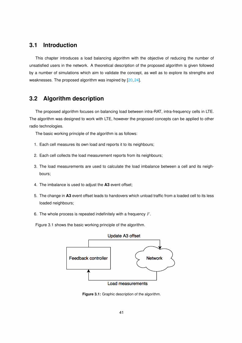
3.1 Introduction
This chapter introduces a load balancing algorithm with the objective of reducing the number of
unsatisfied users in the network. A theoretical description of the proposed algorithm is given followed
by a number of simulations which aim to validate the concept, as well as to explore its strengths and
weaknesses. The proposed algorithm was inspired by [20,24].
3.2 Algorithm description
The proposed algorithm focuses on balancing load between intra-RAT, intra-frequency cells in LTE.
The algorithm was designed to work with LTE, however the proposed concepts can be applied to other
radio technologies.
The basic working principle of the algorithm is as follows:
1. Each cell measures its own load and reports it to its neighbours;
2. Each cell collects the load measurement reports from its neighbours;
3. The load measurements are used to calculate the load imbalance between a cell and its neigh-
bours;
4. The imbalance is used to adjust the A3 event offset;
5. The change in A3 event offset leads to handovers which unload traffic from a loaded cell to its less
loaded neighbours;
6. The whole process is repeated indefinitely with a frequency F .
Figure 3.1 shows the basic working principle of the algorithm.
Figure 3.1: Graphic description of the algorithm.
41

3.2.1 Load measurements
The proposed algorithm uses as an indirect load measurement, the number of unsatisfied users in a
cell at a given time. The number of unsatisfied users is given by the number of users whose throughput
is below the minimum required bitrate for each user. More formally:
Load =∑u ∈ U
1tu<Du, (3.1)
where Du denotes the user’s minimum required bitrate, tu the user’s current throughput, and 1tu<Du
is an indicator function which equals one if the user’s throughput is below the requirement and zero
otherwise.
By using the number of unsatisfied users as a load measurement, it is possible to minimise this
quantity directly. This load measurement is also a performance metric since the less unsatisfied users
in a cell the better.
This particular load measurement was chosen because the relation between direct load measures
(such as percentage of used PRBs) and the network performance is not linear. It is possible for the
network to be using all of its resources and still be performing well from the users’ perspective. By
using the number of unsatisfied users as the load measure, the networks load can be tied directly to its
performance. In addition, in the simulation phase (Section 3.3), for the sake of keeping computational
costs down, the traffic model used for all the UEs was the full-buffer traffic model. This simplification
leads to all of the network’s PRBs being utilised at all times, as a result, using the percentage of used
PRBs or other related quantities makes little sense.
3.2.2 Calculating load imbalance
After each cell measures its own load and its neighbours load, it is necessary to determine the load
imbalance between a cell and its neighbours.
Different vendors allow for the setting of the A3 event offset on a cell basis or on a neighbour relation
basis, this will affect the manner in which the load imbalance between a cell and its neighbours is
calculated.
If the A3 event offset can only be set on a cell basis the load imbalance of a cell is given by:
∆l =Load− f(Loadn1
, Loadn2, ..., LoadnN
)
Load× 100% , (3.2)
where ∆l is the load imbalance, Load is the load of the cell, Loadn1 , Loadn2 , ..., LoadnNare the loads of
the neighbouring cells and f(·) is a function that aggregates the load measures, e.g. mean or maximum
value.
42

If the cell’s load is zero, the imbalance is considered to be zero, this design decision is very important
because it:
1. Prevents two cells from adjusting their handover offsets simultaneously in opposite directions,
causing the effective offset between the two to be twice as large;
2. Constrains the effect of the load balancing algorithm to the overloaded cell and its neighbours,
preventing undesired handovers between two not overloaded cells simply because one of them is
neighbouring an overloaded cell.
If the A3 event offset can be set per neighbour relation the load imbalance is given by:
∆l =Load− Loadn
max(Load, Loadn)× 100% , (3.3)
where Load and Loadn are the loads of the cell and its neighbour respectively. The imbalance is nor-
malised with the respect to the maximum of the two loads in order to obtain symmetrical offsets from the
perspective of the two cells in the neighbouring relation.
Note that cells more loaded than its neighbours will have positive load imbalances and cells less
loaded than its neighbours will have negative load imbalances.
To avoid dividing by zero, if both of the cell’s load is zero then the imbalance is said to be zero.
3.2.3 Adjusting the A3 event offsets
After having calculated the load imbalance between a cell and its neighbours, it is necessary to adjust
the handover offsets which will lead to a better load distribution. Section 3.2.3.A specifies how to adjust
said offsets on a per cell basis and Section 3.2.3.B on a per neighbour relation basis.
3.2.3.A Per cell offset adjustment
If the offset adjustment is to be made on a per cell basis, then by setting the offset and frequency
specific offsets in equation (2.6) to zero, it comes that the A3 event entering condition is:
Mn+Ocn−Ms−Ocs−Hys > 0 . (3.4)
In this case every cell will adjusts its offset Ocs independently. From the cell’s perspective, Ocn is the
Ocs of the neighbouring cell being considered in the A3 event.
43

3.2.3.B Per neighbour relation offset adjustment
If the offset is to be adjusted on per neighbour relation, then by setting the cell and frequency specific
offsets to zero in equation (2.6), it comes that the A3 event entering condition is:
Mn−Ms−Off −Hys > 0 . (3.5)
In this situation the offset Off will be adjusted, this offset only refers to the neighbour relation be-
tween the two cells being considered in the A3 event.
Note that in both cases the offsets that were set to zero need not be zero, however these will not be
adjusted by the algorithm and may interfere with its performance.
3.2.3.C Incrementing the offsets
From equations (3.4) and (3.5) it can be deduced that if a cell is overloaded with respect to a neigh-
bour, the offset Off of the relation or its offset Ocs must decrease in order to make the cell look less
appealing in the power domain, and cause the UEs to enter the A3 event sooner.
In order to do this, the algorithm will increment these offsets in a recursive manner using a stair
function. The function can have has many steps as needed and the steps may have whichever height is
found optimal. An example function is shown in Figure 3.2:
Figure 3.2: Stair function.
The parameters t1, t2, ..., tk denote thresholds after which the increments i1, i2, ..., ik will be added to
the cell’s or neighbour relation offset.
With this function, if the imbalance of a cell is positive then its offset decreases in order to make
the perceived signal from this cell seem weaker, this will trigger the UEs at the cell’s edge to request
44
handovers to neighbouring cells.
To prevent an indefinite increase/decrease in the offset which could lead to RLFs, the maximum
absolute offset value is curbed at a value Maxoffset. In reality there could be another way to prevent
RLFs without curbing the offset, such as adding to the feedback controller a gain controller which would
control the increment based on the number of RLFs in the cell, however, this was left for future work.
3.3 Simulation
To validate the proposed algorithm, several simulations were conducted using the Vienna LTE Sys-
tem Level Simulator [1]. Documentation on how to use the simulator can be found in [54].
This simulator works on the system level, meaning that it simulates multiple UEs and multiple eN-
odeBs at the TTI level. In LTE, one TTI corresponds to one millisecond, meaning that for each simulated
millisecond the simulator calculates the channel conditions for each UE and performs the scheduling of
PRBs in each eNodeB.
This level of detail proved to be too computationally expensive for the desired objectives, as a result
several changes had to be made to the simulator in order to make the simulations computationally
feasible.
3.3.1 Changes made to the simulator
This section gives a brief overview of the changes implemented in the simulator, either for improving
performance or to achieve the desired simulation objectives.
3.3.1.A Macroscopic channel recalculation
The macroscopic channel includes the pathloss and shadow fading components of the channel
model. In the simulator, for each UE all of the channel components are recalculated each millisec-
ond, however, in reality, the macroscopic large-scale channel conditions do not change significantly on
this time scale. This means that there are computational resources being spent on recalculating the
same value, or very close values, repeatedly when it is not necessary.
According to [55] the optimal distance over which to calculate the local average power of the signal
is between 20-40 wavelengths. This is finding is based on the 90% confidence interval with less than 1
dB of error in the estimate.
Because of this, the possibility to only recalculate the macroscopic channel conditions in fixed time
intervals was implemented. For example, the macroscopic channel conditions are calculated at time 0
ms and remain constant until time 200 ms when they will be recalculated. This feature allows to speed
45

up the simulation significantly since the macroscopic channel recalculation took a large portion of the
simulation time.
3.3.1.B Handover module
The simulator did not have handover implemented, UEs remained permanently connected to their
initial cell regardless of the received power.
Since adjusting handover parameters is the key concept of the proposed load balancing algorithm, an
handover module had first to be implemented. The implemented handover module has all the features
described in section 2.4.2, with configurable parameters including:
• Handover hysteresis;
• Time-to-trigger;
• Handover Offsets (Cell, frequency and neighbour relation specific offsets);
• Handover filter coefficient.
All of these parameters can be configured by the user, even though some of them will be changed
by the load balancing algorithm. This module greatly increases the simulator’s capabilities and allows
for much more realistic simulations.
3.3.1.C User walking/driving models
The only walking/driving model available in the vanilla simulator, apart from all UEs reaming still, was
the random walk model, where at each TTI the UEs move in random directions independent of their
movement in the previous TTI. This model is not realistic since in reality the users’ movement tends to
be deliberate and not random.
To validate the load balancing algorithm it was necessary to create load imbalances in the network
while using credible walking/driving models for the users. With this in mind, several new walking/driving
models were introduced in simulator along with some extra features. These models and features are
listed below:
• The ability for users to turn around once they reach the simulation’s edge (before UEs were tele-
ported to a random point);
• The random way-point walking model, where each UE chooses a random direction and moves in
that direction until it reaches the simulation’s edge, where it will ricochet and continue moving in
the new direction;
46

• The hotspot walking model, where users move in the direction of one or more hotspots until they
get there. On arrival, if there is more than one hotspot, the users pick another hotspot at random
and move in its direction. The hotspots are predefined simulation parameters;
• The Manhattan walking model, where users move in a predefined square grid. At an intersection
each of the four directions has an associated probability that the user will choose said direction.
These probabilities are configurable simulation parameters, and can be tuned to create hotspots
or other imbalanced load distributions. In this model, the UEs are only allowed to move in the grid.
In the end, only the last of the implemented models was used since it was the closest to the reality
of user movement in an urban environment.
3.3.1.D General optimisation
To improve the performance of the simulator, several code optimisations were made to the simulator.
These optimisations do not change the behaviour of the code but improve the running time and memory
used to simulate. The optimisations were made based on information returned by the MATLAB profiler,
and are basically the optimization of loops and function calls.
The combination of this optimisation with the macroscopic channel recalculation in larger intervals
led to a considerable decrease in simulation times. Simulation which before had estimated completion
times of weeks, now take only days. It is estimated that simulator became over 10 times faster than
before. As for memory, the result file size decreased from around 20 GB to around 400 MB (for the
desired simulations).
3.3.1.E Load balancing algorithm
Lastly, the load balancing algorithm described in Section 3.2 was implemented in order to test its
performance against the case where no load balancing is used. The implementation of the algorithm
contains a module that measure each cell’s load and another that adjusts the handover offsets based
on the measurements performed.
3.3.2 General parameters
In this section, the general parameters used in the simulations are presented. In Table 3.1 some
macro parameters used in the simulations are shown.
As the bandwidth increases, the simulation’s run time increases due to the scheduler having more
PRBs to allocate. As a result, the bandwidth is only 1.4 MHz in order to keep computational costs down.
As for the network configuration, the simulated network was composed of an hexagonal grid made
up of 7 sites, 21 cells and 420 UEs (20 per cell). The UEs were assumed to be in vehicles with a speed
47
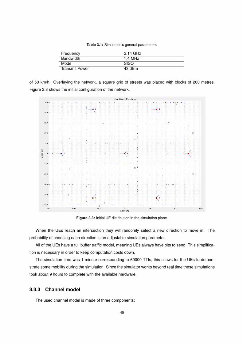
Table 3.1: Simulation’s general parameters.
Frequency 2.14 GHzBandwidth 1.4 MHzMode SISOTransmit Power 43 dBm
of 50 km/h. Overlaying the network, a square grid of streets was placed with blocks of 200 metres.
Figure 3.3 shows the initial configuration of the network.
Figure 3.3: Initial UE distribution in the simulation plane.
When the UEs reach an intersection they will randomly select a new direction to move in. The
probability of choosing each direction is an adjustable simulation parameter.
All of the UEs have a full buffer traffic model, meaning UEs always have bits to send. This simplifica-
tion is necessary in order to keep computation costs down.
The simulation time was 1 minute corresponding to 60000 TTIs, this allows for the UEs to demon-
strate some mobility during the simulation. Since the simulator works beyond real time these simulations
took about 9 hours to complete with the available hardware.
3.3.3 Channel model
The used channel model is made of three components:
48

• Macroscopic pathloss;
• Shadow fading;
• Fast fading or small scale fading.
The first two components fall under the category of slow fading since they vary slowly with time.
Meaning the signal frequency is significantly larger than the frequency of variations in the slow fading
attenuation.
The macroscopic pathloss model used was the COST231 extended Hata model for urban environ-
ments specified in [56].
The shadow fading model used was the Claussen model [57] which generates a log-normally dis-
tributed two dimensional spatially-correlated shadow fading map. The distribution used had a mean of 0
dB and a standard deviation of 8 dB. The standard deviation chosen falls in the middle of the interval of
typical values determined empirically by several different authors [58].
The slow fading part of the channel was recalculated every 20λ which at a UE speed of 50 km/h
results in recalculating the channel every 202 TTIs.
The fast fading model used was the Vehicular A model specified in [59], in addition 7 dB of extra
penetration loss was added to account for the UEs being inside vehicles.
3.3.4 Mobility parameters
The handover time-to-trigger parameter was set to 40 milliseconds and the handover filter coefficient
was set to k = 4 [15].
For the case where no load balancing is used the handover hysteresis is set to 1 dB. This is Ericsson’s
recommendation for cases of high load [15].
For the case where load balancing is used the handover hysteresis is set to 4 dB in order to prevent
the algorithm from causing an increase in ping-pong handovers.
Note that even though the handover hysteresis parameter is different for the two cases, this corre-
sponds to giving the best chance at a good performance for each case (this was verified during the
simulation phase). This means that the performance of the network when no load balancing algorithm
is used is better when the hysteresis is 1 dB rather than 4 dB, and that the performance of the network
when the load balancing algorithm is used is better when the hysteresis is 4 dB rather than 1 dB.
3.3.5 Measuring performance
To measure the performance of the load balancing algorithm it is necessary to compare it to the case
where no load balancing was used. Some comparison metrics for the gain of the algorithm must be
49
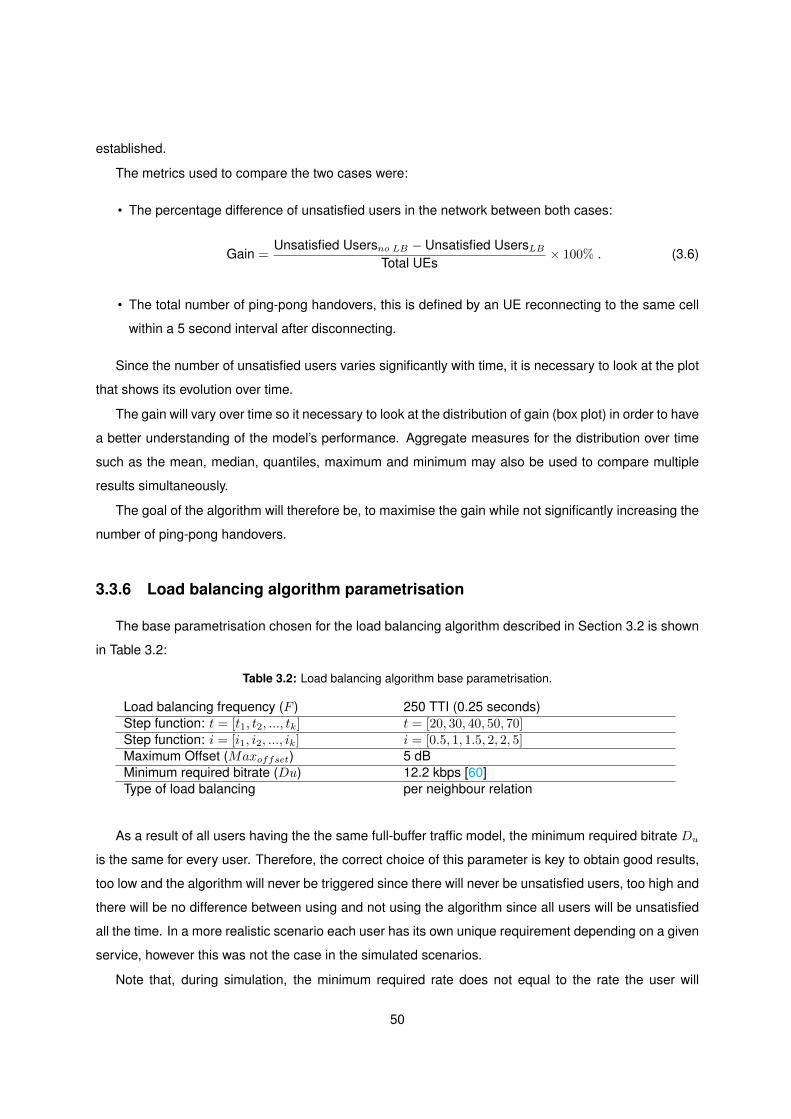
established.
The metrics used to compare the two cases were:
• The percentage difference of unsatisfied users in the network between both cases:
Gain =Unsatisfied Usersno LB − Unsatisfied UsersLB
Total UEs× 100% . (3.6)
• The total number of ping-pong handovers, this is defined by an UE reconnecting to the same cell
within a 5 second interval after disconnecting.
Since the number of unsatisfied users varies significantly with time, it is necessary to look at the plot
that shows its evolution over time.
The gain will vary over time so it necessary to look at the distribution of gain (box plot) in order to have
a better understanding of the model’s performance. Aggregate measures for the distribution over time
such as the mean, median, quantiles, maximum and minimum may also be used to compare multiple
results simultaneously.
The goal of the algorithm will therefore be, to maximise the gain while not significantly increasing the
number of ping-pong handovers.
3.3.6 Load balancing algorithm parametrisation
The base parametrisation chosen for the load balancing algorithm described in Section 3.2 is shown
in Table 3.2:
Table 3.2: Load balancing algorithm base parametrisation.
Load balancing frequency (F ) 250 TTI (0.25 seconds)Step function: t = [t1, t2, ..., tk] t = [20, 30, 40, 50, 70]Step function: i = [i1, i2, ..., ik] i = [0.5, 1, 1.5, 2, 2, 5]Maximum Offset (Maxoffset) 5 dBMinimum required bitrate (Du) 12.2 kbps [60]Type of load balancing per neighbour relation
As a result of all users having the the same full-buffer traffic model, the minimum required bitrate Du
is the same for every user. Therefore, the correct choice of this parameter is key to obtain good results,
too low and the algorithm will never be triggered since there will never be unsatisfied users, too high and
there will be no difference between using and not using the algorithm since all users will be unsatisfied
all the time. In a more realistic scenario each user has its own unique requirement depending on a given
service, however this was not the case in the simulated scenarios.
Note that, during simulation, the minimum required rate does not equal to the rate the user will
50
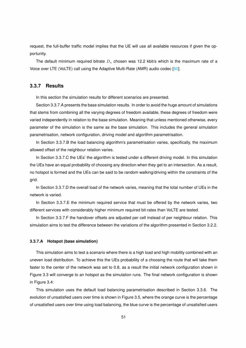
request, the full-buffer traffic model implies that the UE will use all available resources if given the op-
portunity.
The default minimum required bitrate Du chosen was 12.2 kbit/s which is the maximum rate of a
Voice over LTE (VoLTE) call using the Adaptive Multi-Rate (AMR) audio codec [60].
3.3.7 Results
In this section the simulation results for different scenarios are presented.
Section 3.3.7.A presents the base simulation results. In order to avoid the huge amount of simulations
that stems from combining all the varying degrees of freedom available, these degrees of freedom were
varied independently in relation to the base simulation. Meaning that unless mentioned otherwise, every
parameter of the simulation is the same as the base simulation. This includes the general simulation
parametrisation, network configuration, driving model and algorithm parametrisation.
In Section 3.3.7.B the load balancing algorithm’s parametrisation varies, specifically, the maximum
allowed offset of the neighbour relation varies.
In Section 3.3.7.C the UEs’ the algorithm is tested under a different driving model. In this simulation
the UEs have an equal probability of choosing any direction when they get to an intersection. As a result,
no hotspot is formed and the UEs can be said to be random walking/driving within the constraints of the
grid.
In Section 3.3.7.D the overall load of the network varies, meaning that the total number of UEs in the
network is varied.
In Section 3.3.7.E the minimum required service that must be offered by the network varies, two
different services with considerably higher minimum required bit-rates than VoLTE are tested.
In Section 3.3.7.F the handover offsets are adjusted per cell instead of per neighbour relation. This
simulation aims to test the difference between the variations of the algorithm presented in Section 3.2.2.
3.3.7.A Hotspot (base simulation)
This simulation aims to test a scenario where there is a high load and high mobility combined with an
uneven load distribution. To achieve this the UEs probability of a choosing the route that will take them
faster to the center of the network was set to 0.8, as a result the initial network configuration shown in
Figure 3.3 will converge to an hotspot as the simulation runs. The final network configuration is shown
in Figure 3.4:
This simulation uses the default load balancing parametrisation described in Section 3.3.6. The
evolution of unsatisfied users over time is shown in Figure 3.5, where the orange curve is the percentage
of unsatisfied users over time using load balancing, the blue curve is the percentage of unsatisfied users
51
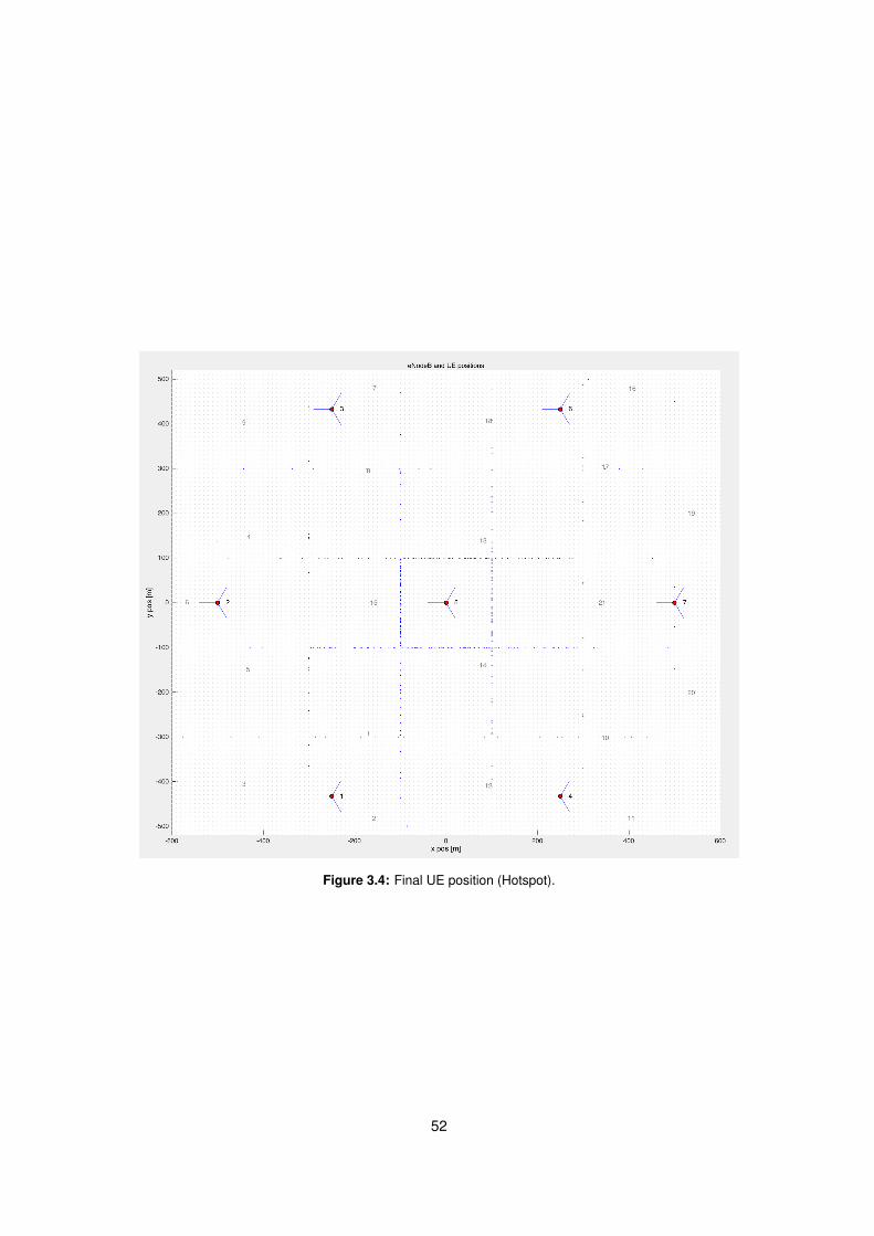
Figure 3.4: Final UE position (Hotspot).
52
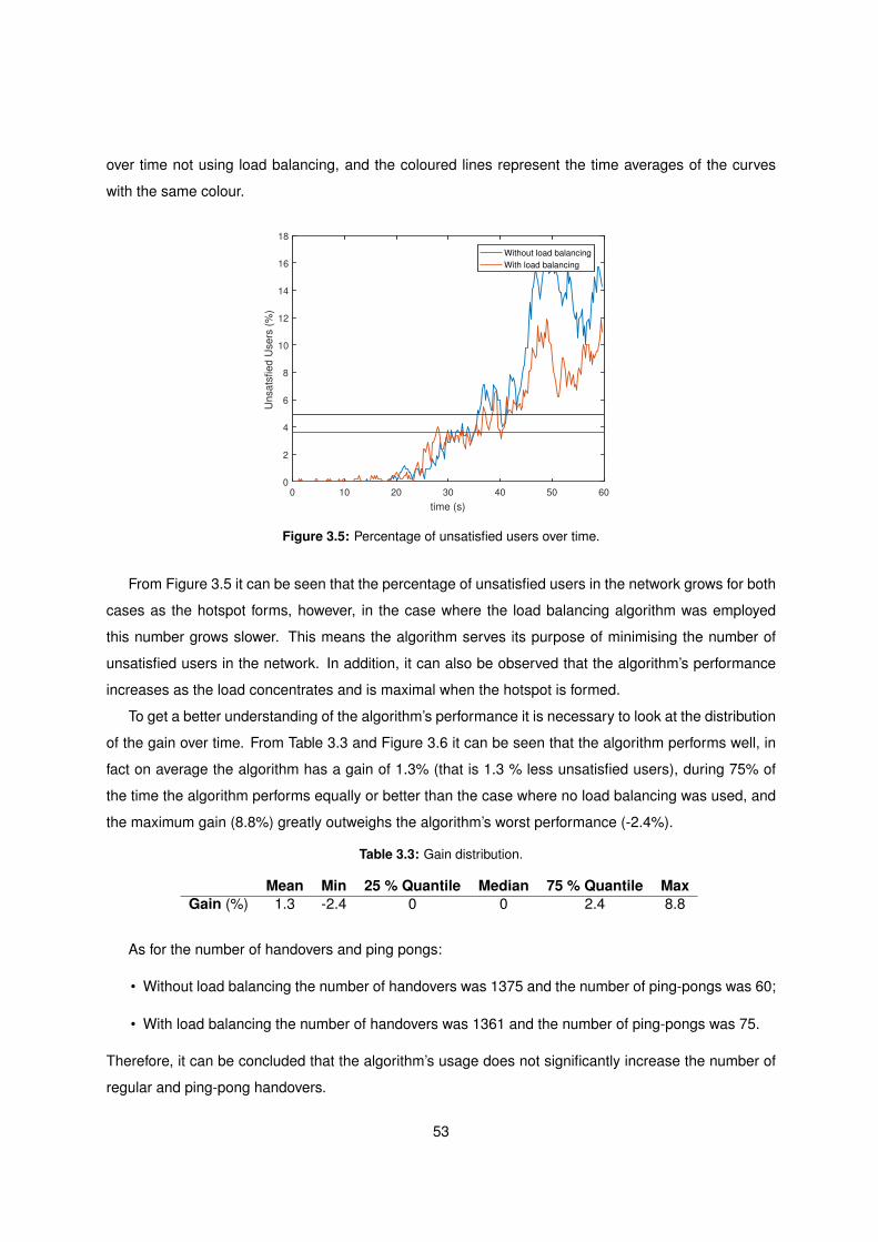
over time not using load balancing, and the coloured lines represent the time averages of the curves
with the same colour.
0 10 20 30 40 50 60
time (s)
0
2
4
6
8
10
12
14
16
18
Unsats
fied U
sers
(%
)
Without load balancing
With load balancing
Figure 3.5: Percentage of unsatisfied users over time.
From Figure 3.5 it can be seen that the percentage of unsatisfied users in the network grows for both
cases as the hotspot forms, however, in the case where the load balancing algorithm was employed
this number grows slower. This means the algorithm serves its purpose of minimising the number of
unsatisfied users in the network. In addition, it can also be observed that the algorithm’s performance
increases as the load concentrates and is maximal when the hotspot is formed.
To get a better understanding of the algorithm’s performance it is necessary to look at the distribution
of the gain over time. From Table 3.3 and Figure 3.6 it can be seen that the algorithm performs well, in
fact on average the algorithm has a gain of 1.3% (that is 1.3 % less unsatisfied users), during 75% of
the time the algorithm performs equally or better than the case where no load balancing was used, and
the maximum gain (8.8%) greatly outweighs the algorithm’s worst performance (-2.4%).
Table 3.3: Gain distribution.
Mean Min 25 % Quantile Median 75 % Quantile MaxGain (%) 1.3 -2.4 0 0 2.4 8.8
As for the number of handovers and ping pongs:
• Without load balancing the number of handovers was 1375 and the number of ping-pongs was 60;
• With load balancing the number of handovers was 1361 and the number of ping-pongs was 75.
Therefore, it can be concluded that the algorithm’s usage does not significantly increase the number of
regular and ping-pong handovers.
53
1
-2
-1
0
1
2
3
4
5
6
7
Gain
(%
)
Figure 3.6: Gain distribution’s box plot.
In the following sections, in order to present results compactly only the mean and maximum gains
will be presented, since these are representative of the overall performance and the performance when
the hotspot is formed. In addition, all of the following simulations will be similar to this one except for one
varying parameter which is the one under analysis.
3.3.7.B Varying parametrisation
In this section the base simulation was kept changing only the load balancing algorithm’s parametri-
sation, specifically the parameter Maxoffset which dictates how much the algorithm is allowed to move
the handover offset by. This parameter was allowed to take the values [1, 2, 3, 4, 5, 6, 7, 8, 9] dB, the
simulations were run and then compared with the base simulation where no load balancing was used.
The results for the variation of the mean gain, maximum gain and number of ping-pongs with the
variation of the Maxoffset parameter are show in Figures 3.7(a) and 3.7(b).
From Figure 3.7(a) it can be seen that the mean gain peaks when Maxoffset is 6 dB, however, from
Figure 3.7(b) it can concluded that as this parameter increases, the number of ping-pongs increases
exponentially, even doubling between 5 and 7 dB. Because of this, it is safe to assume that the optimal
value of the parameter Maxoffset is a low one closer to 4 dB, since for higher values the number of
ping-pongs increases too drastically and the variation of this parameter seems not to have a significant
impact on the algorithm’s gain.
If however, the load balancing algorithm was working in conjunction with a mobility robustness op-
timisation algorithm, this parameter would not be a concern since the mobility robustness optimisation
algorithm would curb it when the number of ping-pongs increased.
54
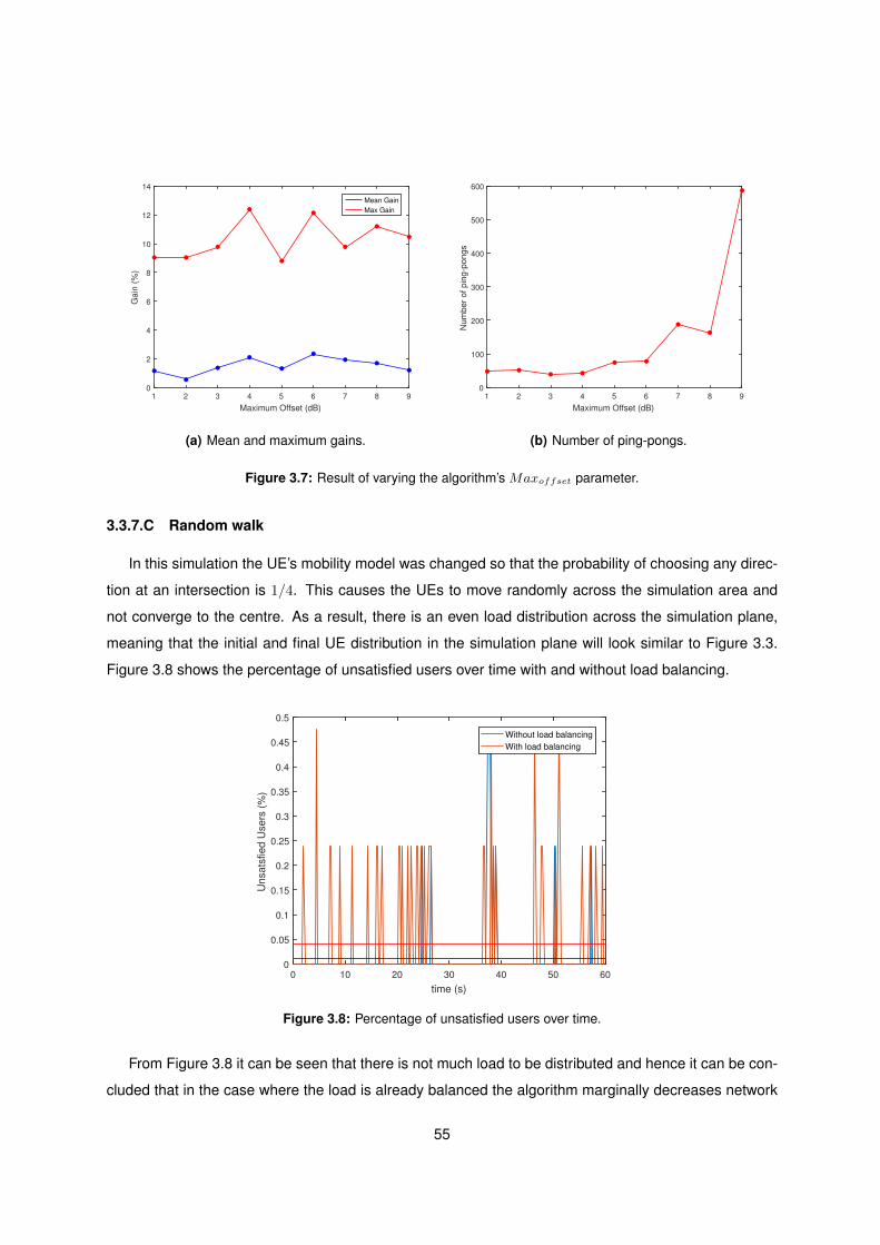
1 2 3 4 5 6 7 8 9
Maximum Offset (dB)
0
2
4
6
8
10
12
14
Ga
in (
%)
Mean Gain
Max Gain
(a) Mean and maximum gains.
1 2 3 4 5 6 7 8 9
Maximum Offset (dB)
0
100
200
300
400
500
600
Nu
mb
er
of
pin
g-p
on
gs
(b) Number of ping-pongs.
Figure 3.7: Result of varying the algorithm’s Maxoffset parameter.
3.3.7.C Random walk
In this simulation the UE’s mobility model was changed so that the probability of choosing any direc-
tion at an intersection is 1/4. This causes the UEs to move randomly across the simulation area and
not converge to the centre. As a result, there is an even load distribution across the simulation plane,
meaning that the initial and final UE distribution in the simulation plane will look similar to Figure 3.3.
Figure 3.8 shows the percentage of unsatisfied users over time with and without load balancing.
0 10 20 30 40 50 60
time (s)
0
0.05
0.1
0.15
0.2
0.25
0.3
0.35
0.4
0.45
0.5
Unsats
fied U
sers
(%
)
Without load balancing
With load balancing
Figure 3.8: Percentage of unsatisfied users over time.
From Figure 3.8 it can be seen that there is not much load to be distributed and hence it can be con-
cluded that in the case where the load is already balanced the algorithm marginally decreases network
55

performance. Even though the decrease in performance is not significant, it can be concluded that there
is no point in employing the load balancing algorithm in cases where there is no load to be balanced.
3.3.7.D Varying load
In this section the performance of the algorithm will be tested under different network load configu-
rations. Since the traffic model used in the simulations is the full-buffer model, the network’s load will
always be 1, that is full utilization of network resources. Because of this, it is necessary to introduce
the concept of virtual load [24, 61], the virtual load of the network is the amount of PRBs necessary
to serve Nu users with a given minimum rate Du given MPRP available PRBs and a spectral effi-
ciency R(SINRu). Equation (3.7) expresses the virtual load as function of these parameters, where
BW = 180 kHz is the bandwidth of one PRB in LTE.
ρ =1
MPRB×Nu ×
Du
R(SINRu)×BW. (3.7)
Note that even though the number of users Nu and the minimum required rate Du are constant,
because the load of the network is not balanced, it varies over time depending on the cell. As a result it
is necessary to look at two cases:
• The case where the load is fully distributed: MPRB = 21× 6 ;
• The case where the load is fully concentrated in a hotspot MPRB = 6 .
Where 6 is the number of available PRBs for one cell using a bandwidth of 1.4 MHz and 21 is the
number of cells in the network. The spectral efficiency R(SINRu) was taken from the simulations’
results. If the virtual load of the network is greater than one, than this means that the network needs
more resources to serve its users at the rate Du than it actually has. For example, if ρ = 2 than the
network needs twice the resources it has to be able to properly serve its users.
The number of UEs/cell was set to [10, 15, 20, 25], the simulations with and without load balancing
were run, and the respective virtual loads were calculated. The mean and maximum gain of the load
balancing algorithm for each one of the load configurations is plotted in Figures 3.9(a) and 3.9(b).
In Figure 3.9(a) the x axis is expressed in terms of UEs/cell (there are 21 cells in the network) and in
Figure 3.9(b) the x axis is expressed in terms of both the network’s overall virtual load and the hotspot’s
virtual load (concentrated load).
From these results it can be seen that the gain of the algorithm grows as the network load increases,
in fact the gain is maximum when the concentrated virtual load is thrice what the network can bare.
To better explain why this is the case, Figures 3.10(a) and 3.10(b) shows the evolution over time in
the percentage of unsatisfied users for a load of 10 UEs/cell and 25 UEs/cell.
56
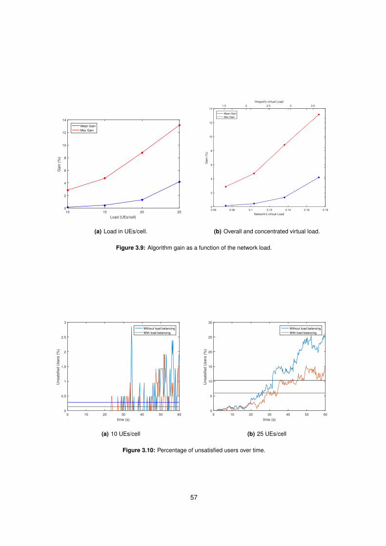
10 15 20 25
Load (UEs/cell)
0
2
4
6
8
10
12
14
Ga
in (
%)
Mean Gain
Max Gain
(a) Load in UEs/cell.
0.06 0.08 0.1 0.12 0.14 0.16 0.18
Network's virtual Load
0
2
4
6
8
10
12
14
Ga
in (
%)
Mean Gain
Max Gain
1.5 2 2.5 3 3.5
Hospot's virtual Load
(b) Overall and concentrated virtual load.
Figure 3.9: Algorithm gain as a function of the network load.
0 10 20 30 40 50 60
time (s)
0
0.5
1
1.5
2
2.5
3
Un
sa
tsfie
d U
se
rs (
%)
Without load balancing
With load balancing
(a) 10 UEs/cell
0 10 20 30 40 50 60
time (s)
0
5
10
15
20
25
30
Un
sa
tsfie
d U
se
rs (
%)
Without load balancing
With load balancing
(b) 25 UEs/cell
Figure 3.10: Percentage of unsatisfied users over time.
57
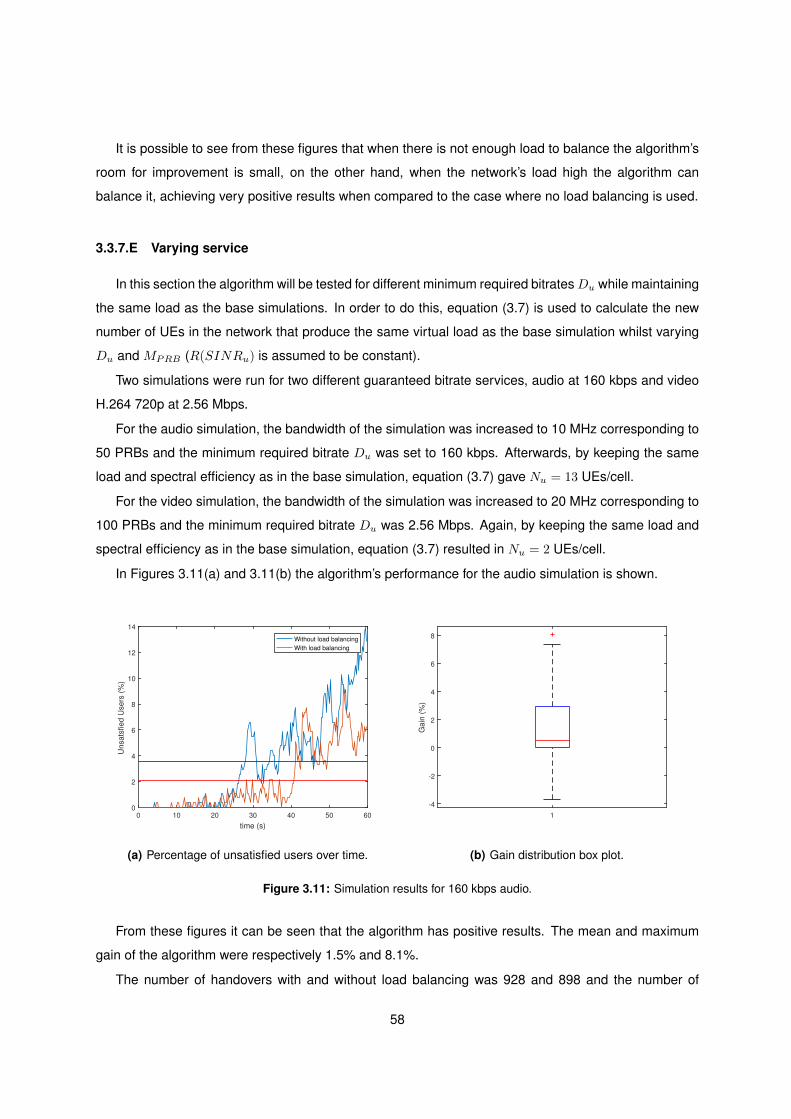
It is possible to see from these figures that when there is not enough load to balance the algorithm’s
room for improvement is small, on the other hand, when the network’s load high the algorithm can
balance it, achieving very positive results when compared to the case where no load balancing is used.
3.3.7.E Varying service
In this section the algorithm will be tested for different minimum required bitratesDu while maintaining
the same load as the base simulations. In order to do this, equation (3.7) is used to calculate the new
number of UEs in the network that produce the same virtual load as the base simulation whilst varying
Du and MPRB (R(SINRu) is assumed to be constant).
Two simulations were run for two different guaranteed bitrate services, audio at 160 kbps and video
H.264 720p at 2.56 Mbps.
For the audio simulation, the bandwidth of the simulation was increased to 10 MHz corresponding to
50 PRBs and the minimum required bitrate Du was set to 160 kbps. Afterwards, by keeping the same
load and spectral efficiency as in the base simulation, equation (3.7) gave Nu = 13 UEs/cell.
For the video simulation, the bandwidth of the simulation was increased to 20 MHz corresponding to
100 PRBs and the minimum required bitrate Du was 2.56 Mbps. Again, by keeping the same load and
spectral efficiency as in the base simulation, equation (3.7) resulted in Nu = 2 UEs/cell.
In Figures 3.11(a) and 3.11(b) the algorithm’s performance for the audio simulation is shown.
0 10 20 30 40 50 60
time (s)
0
2
4
6
8
10
12
14
Un
sa
tsfie
d U
se
rs (
%)
Without load balancing
With load balancing
(a) Percentage of unsatisfied users over time.
1
-4
-2
0
2
4
6
8
Ga
in (
%)
(b) Gain distribution box plot.
Figure 3.11: Simulation results for 160 kbps audio.
From these figures it can be seen that the algorithm has positive results. The mean and maximum
gain of the algorithm were respectively 1.5% and 8.1%.
The number of handovers with and without load balancing was 928 and 898 and the number of
58
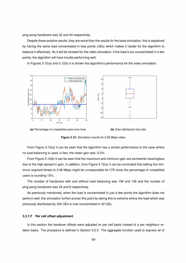
ping-pong handovers was 32 and 34 respectively.
Despite these positive results, they are worst than the results for the base simulation, this is explained
by having the same load concentrated in less points (UEs) which makes it harder for the algorithm to
balance it effectively. As it will be showed for the video simulation, if the load is too concentrated in a few
points, the algorithm will have trouble performing well.
In Figures 3.12(a) and 3.12(b) it is shown the algorithm’s performance for the video simulation.
0 10 20 30 40 50 60
time (s)
0
5
10
15
20
25
30
35
40
45
Un
sa
tsfie
d U
se
rs (
%)
Without load balancing
With load balancing
(a) Percentage of unsatisfied users over time.
1
-25
-20
-15
-10
-5
0
5
10
15
Ga
in (
%)
(b) Gain distribution box plot.
Figure 3.12: Simulation results for 2.56 Mbps video.
From Figure 3.12(a) it can be seen that the algorithm has a similar performance to the case where
no load balancing is used, in fact, the mean gain was -0.2%.
From Figure 3.12(b) it can be seen that the maximum and minimum gain are somewhat meaningless
due to the high spread in gain, in addition, from Figure 3.12(a) it can be concluded that setting the min-
imum required bitrate to 2.56 Mbps might be unreasonable for LTE since the percentage of unsatisfied
users is rounding 15%.
The number of handovers with and without load balancing was 156 and 136 and the number of
ping-pong handovers was 34 and 6 respectively.
As previously mentioned, when the load is concentrated in just a few points the algorithm does not
perform well, this simulation further proves this point by taking this to extreme where the load which was
previously distributed by 420 UEs is now concentrated in 42 UEs.
3.3.7.F Per cell offset adjustment
In this section the handover offsets were adjusted on per cell basis instead of a per neighbour re-
lation basis. The procedure is defined in Section 3.2.3. The aggregate function used to express all of
59
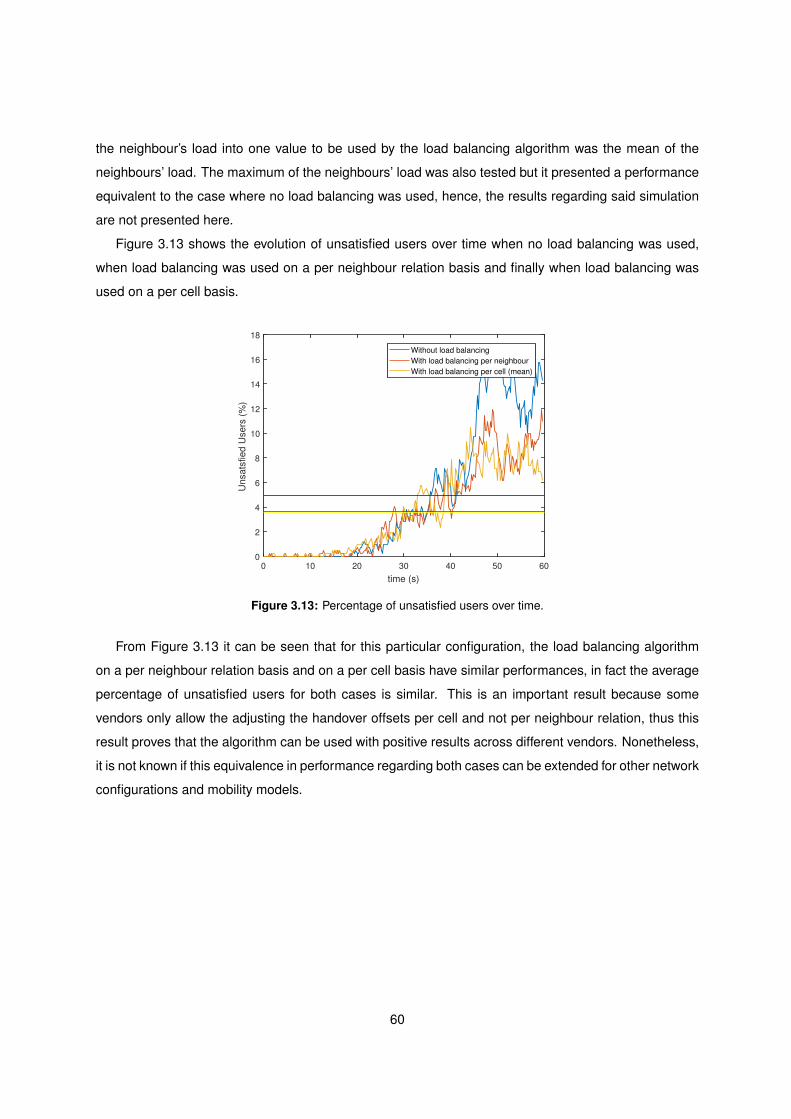
the neighbour’s load into one value to be used by the load balancing algorithm was the mean of the
neighbours’ load. The maximum of the neighbours’ load was also tested but it presented a performance
equivalent to the case where no load balancing was used, hence, the results regarding said simulation
are not presented here.
Figure 3.13 shows the evolution of unsatisfied users over time when no load balancing was used,
when load balancing was used on a per neighbour relation basis and finally when load balancing was
used on a per cell basis.
0 10 20 30 40 50 60
time (s)
0
2
4
6
8
10
12
14
16
18
Unsats
fied U
sers
(%
)
Without load balancing
With load balancing per neighbour
With load balancing per cell (mean)
Figure 3.13: Percentage of unsatisfied users over time.
From Figure 3.13 it can be seen that for this particular configuration, the load balancing algorithm
on a per neighbour relation basis and on a per cell basis have similar performances, in fact the average
percentage of unsatisfied users for both cases is similar. This is an important result because some
vendors only allow the adjusting the handover offsets per cell and not per neighbour relation, thus this
result proves that the algorithm can be used with positive results across different vendors. Nonetheless,
it is not known if this equivalence in performance regarding both cases can be extended for other network
configurations and mobility models.
60
4Forecasting
Contents
4.1 Introduction . . . . . . . . . . . . . . . . . . . . . . . . . . . . . . . . . . . . . . . . . . 63
4.2 Results . . . . . . . . . . . . . . . . . . . . . . . . . . . . . . . . . . . . . . . . . . . . . 64
4.3 Aggregate results . . . . . . . . . . . . . . . . . . . . . . . . . . . . . . . . . . . . . . . 68
4.4 Practical considerations . . . . . . . . . . . . . . . . . . . . . . . . . . . . . . . . . . . 72
4.5 Special cases . . . . . . . . . . . . . . . . . . . . . . . . . . . . . . . . . . . . . . . . . 73
61

62
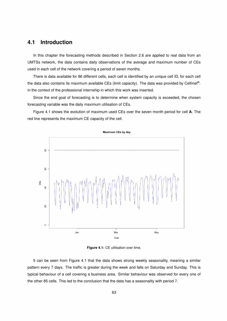
4.1 Introduction
In this chapter the forecasting methods described in Section 2.6 are applied to real data from an
UMTSs network, the data contains daily observations of the average and maximum number of CEs
used in each cell of the network covering a period of seven months.
There is data available for 86 different cells, each cell is identified by an unique cell ID, for each cell
the data also contains its maximum available CEs (limit capacity). The data was provided by Celfinet®.
in the context of the professional internship in which this work was inserted.
Since the end goal of forecasting is to determine when system capacity is exceeded, the chosen
forecasting variable was the daily maximum utilisation of CEs.
Figure 4.1 shows the evolution of maximum used CEs over the seven month period for cell A. The
red line represents the maximum CE capacity of the cell.
Figure 4.1: CE utilisation over time.
It can be seen from Figure 4.1 that the data shows strong weekly seasonality, meaning a similar
pattern every 7 days. The traffic is greater during the week and falls on Saturday and Sunday. This is
typical behaviour of a cell covering a business area. Similar behaviour was observed for every one of
the other 85 cells. This led to the conclusion that the data has a seasonality with period 7.
63
The data was divided into a training and test set, the training set comprises of the fist five months of
the data (70%) and the test set the last two (30%), this means that the forecasting horizon is two months.
The following models were applied:
• Average method;
• Naıve method;
• Seasonal Naıve method;
• Seasonal ARIMA;
• STL decomposition.
For the seasonal models the seasonal period used was 7. In addition, for models that allow the use
of external regressors a binary array denoting whether a given day was an holiday or not was used in
order to increase accuracy.
When fitting the S-ARIMA model a controlled automated fit was used, the seasonal differencing
parameter D was set to 1 and then a model search based on the AICc criterion was performed. In the
STL decomposition model an ARIMA model was used to forecast the trend, this model was again fitted
automatically using the AICc criterion.
4.2 Results
The code for this section was developed in R [62] using the the following additional packages: [63–
68].
This section presents the forecasting results obtained for cell A using the different forecasting meth-
ods mentioned before. When using forecasting methods, it is key to visualise the data and make a
graphical evaluation of the obtained results.
Figures 4.2 and 4.3 show the forecasting results for the average and naıve methods respectively. The
blue line represents the forecasts and the black/red line the actual recorded observations. The shaded
regions represent the 80% (dark blue) and 95% (grey) confidence intervals of the forecast. Both these
methods are very simple, the first simply predicts the average value of the observations, and the second
simply predicts the value of the last observation. Because of this, the expectation for the obtained results
was never vary high, however, even though both methods predict a constant value, the average method
gives much narrower and seemingly more accurate confidence intervals.
Figure 4.4 shows the forecasting result for the seasonal naıve method. This method always predicts
the last observed period, it is possible to see that just adding a seasonal component to the model greatly
increases accuracy of the forecast. However, this method still has large and increasing confidence
64
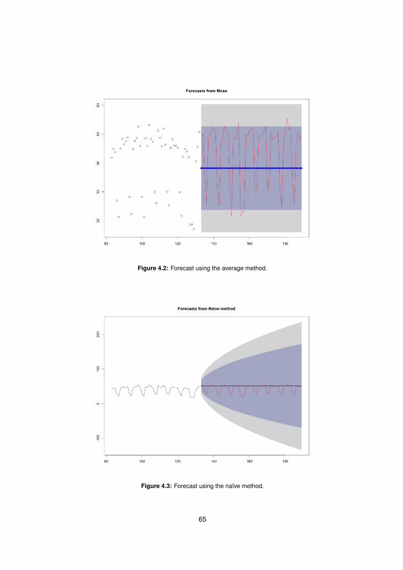
Figure 4.2: Forecast using the average method.
Figure 4.3: Forecast using the naıve method.
65
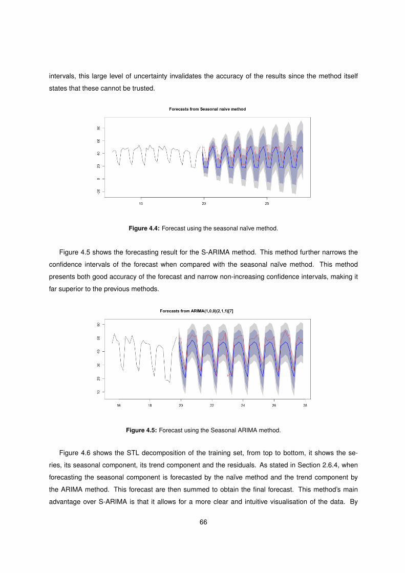
intervals, this large level of uncertainty invalidates the accuracy of the results since the method itself
states that these cannot be trusted.
Figure 4.4: Forecast using the seasonal naıve method.
Figure 4.5 shows the forecasting result for the S-ARIMA method. This method further narrows the
confidence intervals of the forecast when compared with the seasonal naıve method. This method
presents both good accuracy of the forecast and narrow non-increasing confidence intervals, making it
far superior to the previous methods.
Figure 4.5: Forecast using the Seasonal ARIMA method.
Figure 4.6 shows the STL decomposition of the training set, from top to bottom, it shows the se-
ries, its seasonal component, its trend component and the residuals. As stated in Section 2.6.4, when
forecasting the seasonal component is forecasted by the naıve method and the trend component by
the ARIMA method. This forecast are then summed to obtain the final forecast. This method’s main
advantage over S-ARIMA is that it allows for a more clear and intuitive visualisation of the data. By
66
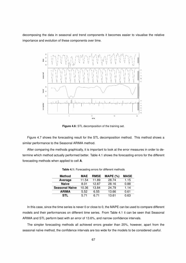
decomposing the data in seasonal and trend components it becomes easier to visualise the relative
importance and evolution of these components over time.
Figure 4.6: STL decomposition of the training set.
Figure 4.7 shows the forecasting result for the STL decomposition method. This method shows a
similar performance to the Seasonal ARIMA method.
After comparing the methods graphically, it is important to look at the error measures in order to de-
termine which method actually performed better. Table 4.1 shows the forecasting errors for the different
forecasting methods when applied to cell A.
Table 4.1: Forecasting errors for different methods
Method MAE RMSE MAPE (%) MASEAverage 11.54 11.89 28.74 1.15
Naive 8.01 12.87 28.16 0.88Seasonal Naive 10.36 13.84 24.79 1.14
ARIMA 5.52 6.55 13.66 0.61STL 5.71 6.71 13.61 0.63
In this case, since the time series is never 0 or close to 0, the MAPE can be used to compare different
models and their performances on different time series. From Table 4.1 it can be seen that Seasonal
ARIMA and STL perform best with an error of 13.6%, and narrow confidence intervals.
The simpler forecasting methods all achieved errors greater than 20%, however, apart from the
seasonal naıve method, the confidence intervals are too wide for the models to be considered useful.
67
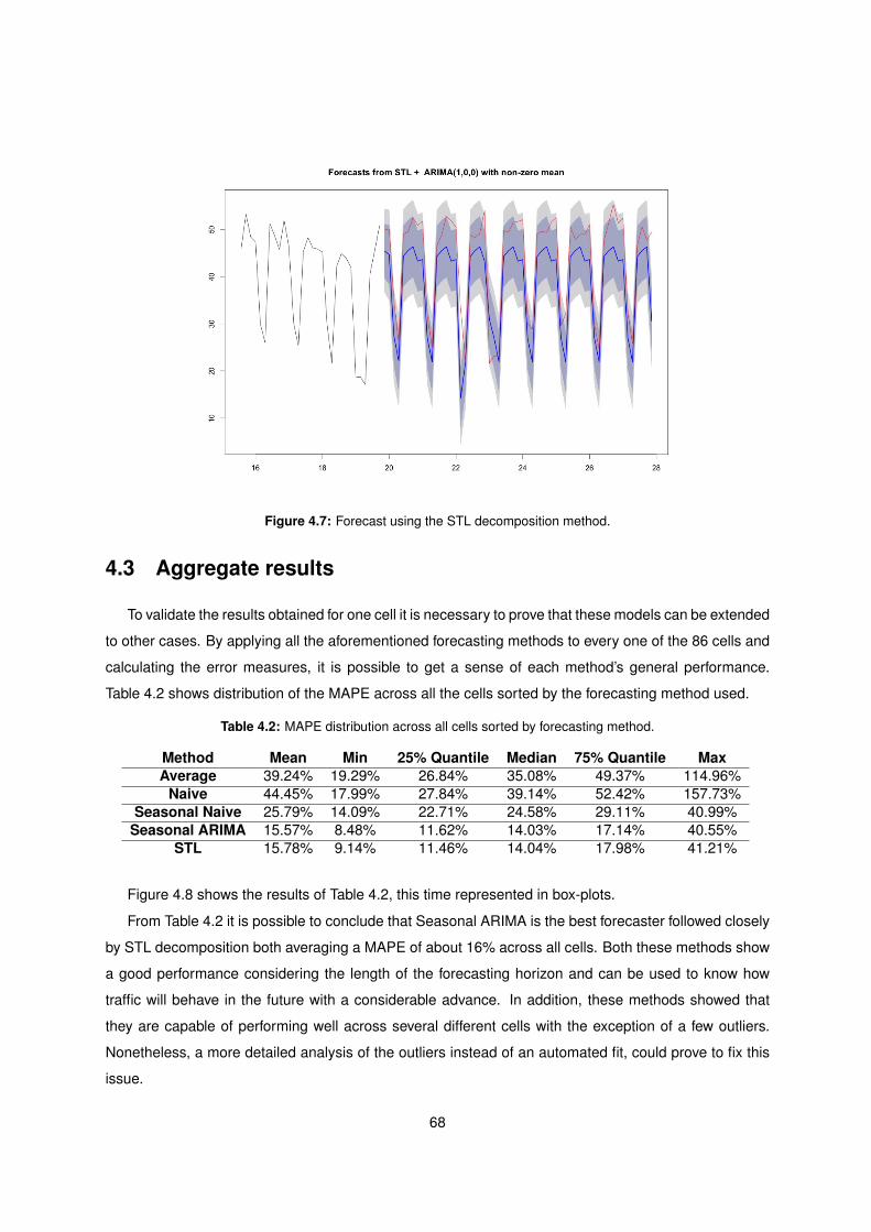
Figure 4.7: Forecast using the STL decomposition method.
4.3 Aggregate results
To validate the results obtained for one cell it is necessary to prove that these models can be extended
to other cases. By applying all the aforementioned forecasting methods to every one of the 86 cells and
calculating the error measures, it is possible to get a sense of each method’s general performance.
Table 4.2 shows distribution of the MAPE across all the cells sorted by the forecasting method used.
Table 4.2: MAPE distribution across all cells sorted by forecasting method.
Method Mean Min 25% Quantile Median 75% Quantile MaxAverage 39.24% 19.29% 26.84% 35.08% 49.37% 114.96%
Naive 44.45% 17.99% 27.84% 39.14% 52.42% 157.73%Seasonal Naive 25.79% 14.09% 22.71% 24.58% 29.11% 40.99%
Seasonal ARIMA 15.57% 8.48% 11.62% 14.03% 17.14% 40.55%STL 15.78% 9.14% 11.46% 14.04% 17.98% 41.21%
Figure 4.8 shows the results of Table 4.2, this time represented in box-plots.
From Table 4.2 it is possible to conclude that Seasonal ARIMA is the best forecaster followed closely
by STL decomposition both averaging a MAPE of about 16% across all cells. Both these methods show
a good performance considering the length of the forecasting horizon and can be used to know how
traffic will behave in the future with a considerable advance. In addition, these methods showed that
they are capable of performing well across several different cells with the exception of a few outliers.
Nonetheless, a more detailed analysis of the outliers instead of an automated fit, could prove to fix this
issue.
68
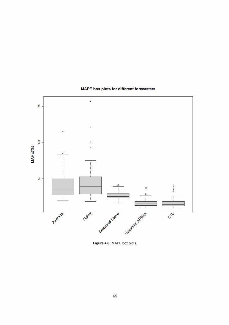
Figure 4.8: MAPE box plots.
69
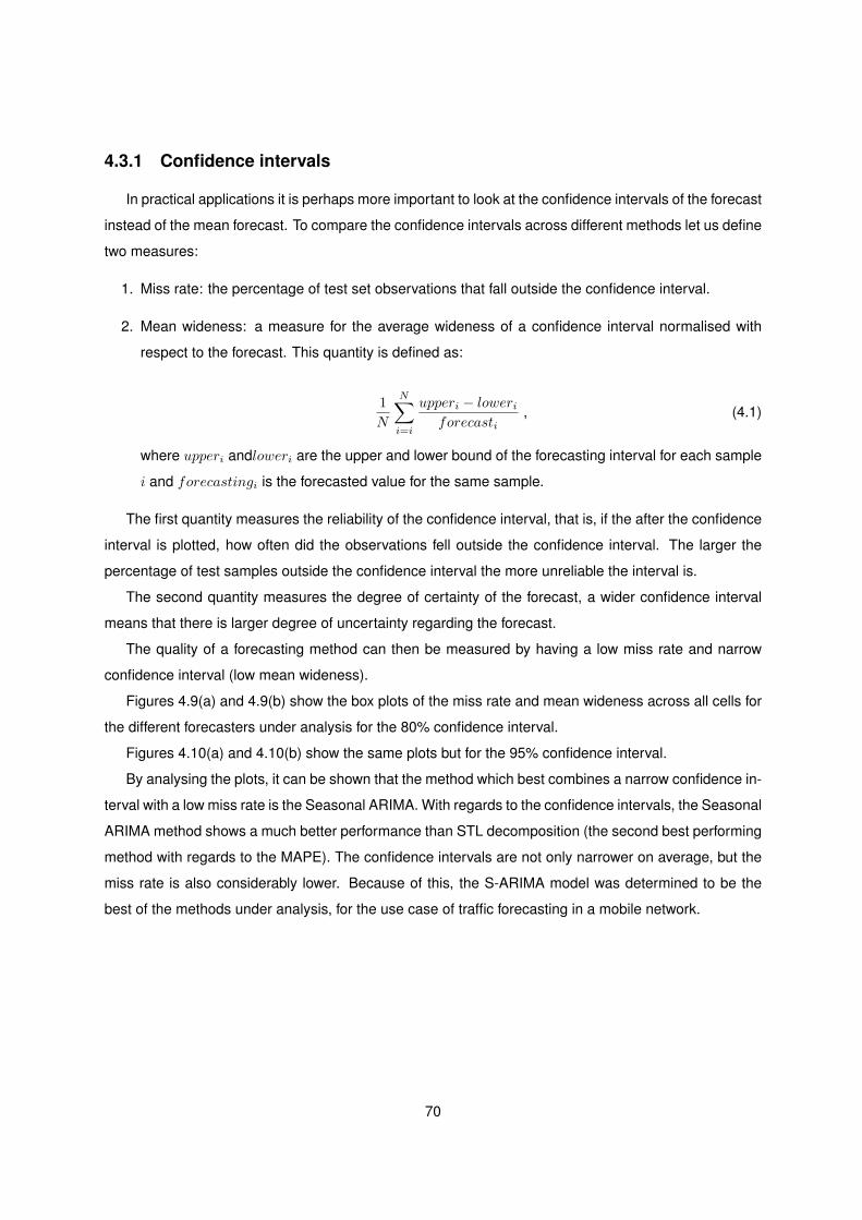
4.3.1 Confidence intervals
In practical applications it is perhaps more important to look at the confidence intervals of the forecast
instead of the mean forecast. To compare the confidence intervals across different methods let us define
two measures:
1. Miss rate: the percentage of test set observations that fall outside the confidence interval.
2. Mean wideness: a measure for the average wideness of a confidence interval normalised with
respect to the forecast. This quantity is defined as:
1
N
N∑i=i
upperi − loweriforecasti
, (4.1)
where upperi andloweri are the upper and lower bound of the forecasting interval for each sample
i and forecastingi is the forecasted value for the same sample.
The first quantity measures the reliability of the confidence interval, that is, if the after the confidence
interval is plotted, how often did the observations fell outside the confidence interval. The larger the
percentage of test samples outside the confidence interval the more unreliable the interval is.
The second quantity measures the degree of certainty of the forecast, a wider confidence interval
means that there is larger degree of uncertainty regarding the forecast.
The quality of a forecasting method can then be measured by having a low miss rate and narrow
confidence interval (low mean wideness).
Figures 4.9(a) and 4.9(b) show the box plots of the miss rate and mean wideness across all cells for
the different forecasters under analysis for the 80% confidence interval.
Figures 4.10(a) and 4.10(b) show the same plots but for the 95% confidence interval.
By analysing the plots, it can be shown that the method which best combines a narrow confidence in-
terval with a low miss rate is the Seasonal ARIMA. With regards to the confidence intervals, the Seasonal
ARIMA method shows a much better performance than STL decomposition (the second best performing
method with regards to the MAPE). The confidence intervals are not only narrower on average, but the
miss rate is also considerably lower. Because of this, the S-ARIMA model was determined to be the
best of the methods under analysis, for the use case of traffic forecasting in a mobile network.
70
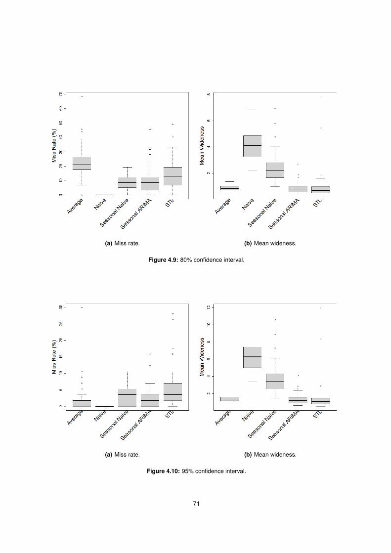
(a) Miss rate. (b) Mean wideness.
Figure 4.9: 80% confidence interval.
(a) Miss rate. (b) Mean wideness.
Figure 4.10: 95% confidence interval.
71
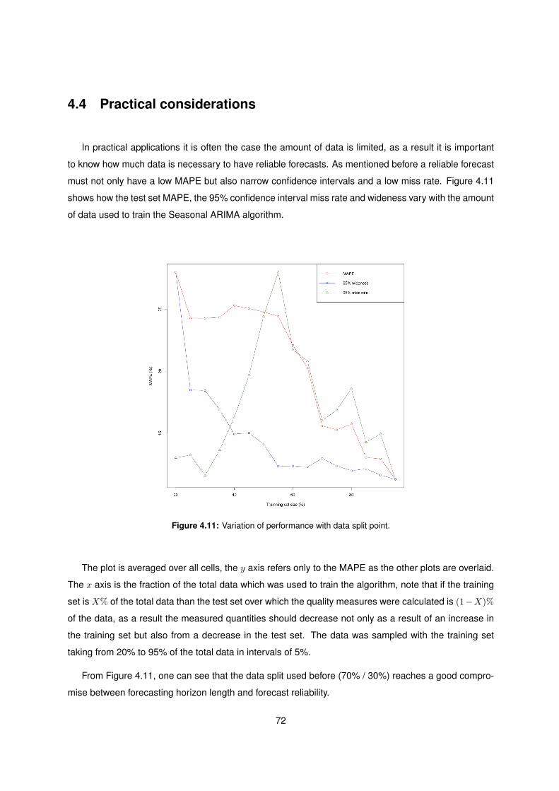
4.4 Practical considerations
In practical applications it is often the case the amount of data is limited, as a result it is important
to know how much data is necessary to have reliable forecasts. As mentioned before a reliable forecast
must not only have a low MAPE but also narrow confidence intervals and a low miss rate. Figure 4.11
shows how the test set MAPE, the 95% confidence interval miss rate and wideness vary with the amount
of data used to train the Seasonal ARIMA algorithm.
Figure 4.11: Variation of performance with data split point.
The plot is averaged over all cells, the y axis refers only to the MAPE as the other plots are overlaid.
The x axis is the fraction of the total data which was used to train the algorithm, note that if the training
set is X% of the total data than the test set over which the quality measures were calculated is (1−X)%
of the data, as a result the measured quantities should decrease not only as a result of an increase in
the training set but also from a decrease in the test set. The data was sampled with the training set
taking from 20% to 95% of the total data in intervals of 5%.
From Figure 4.11, one can see that the data split used before (70% / 30%) reaches a good compro-
mise between forecasting horizon length and forecast reliability.
72
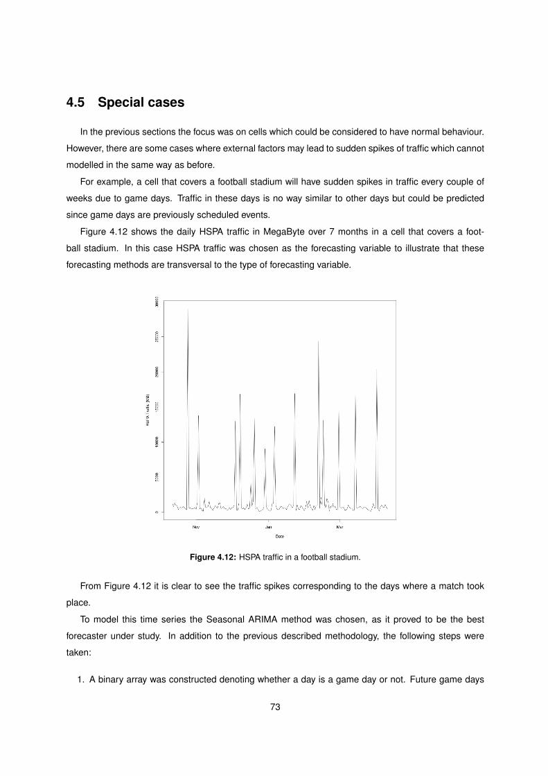
4.5 Special cases
In the previous sections the focus was on cells which could be considered to have normal behaviour.
However, there are some cases where external factors may lead to sudden spikes of traffic which cannot
modelled in the same way as before.
For example, a cell that covers a football stadium will have sudden spikes in traffic every couple of
weeks due to game days. Traffic in these days is no way similar to other days but could be predicted
since game days are previously scheduled events.
Figure 4.12 shows the daily HSPA traffic in MegaByte over 7 months in a cell that covers a foot-
ball stadium. In this case HSPA traffic was chosen as the forecasting variable to illustrate that these
forecasting methods are transversal to the type of forecasting variable.
Figure 4.12: HSPA traffic in a football stadium.
From Figure 4.12 it is clear to see the traffic spikes corresponding to the days where a match took
place.
To model this time series the Seasonal ARIMA method was chosen, as it proved to be the best
forecaster under study. In addition to the previous described methodology, the following steps were
taken:
1. A binary array was constructed denoting whether a day is a game day or not. Future game days
73
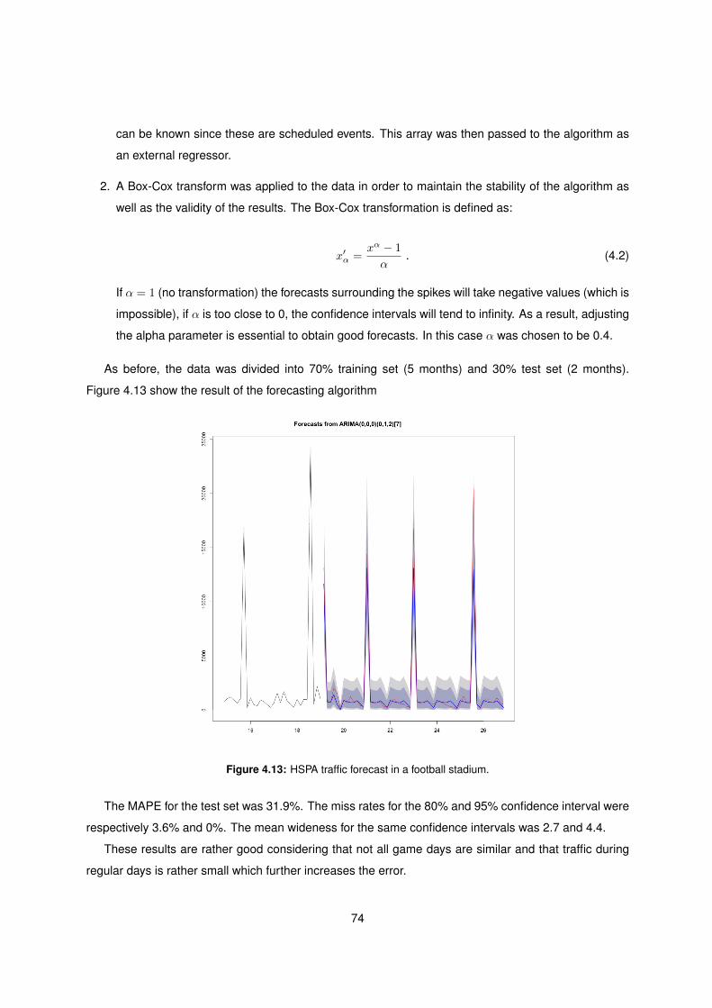
can be known since these are scheduled events. This array was then passed to the algorithm as
an external regressor.
2. A Box-Cox transform was applied to the data in order to maintain the stability of the algorithm as
well as the validity of the results. The Box-Cox transformation is defined as:
x′α =xα − 1
α. (4.2)
If α = 1 (no transformation) the forecasts surrounding the spikes will take negative values (which is
impossible), if α is too close to 0, the confidence intervals will tend to infinity. As a result, adjusting
the alpha parameter is essential to obtain good forecasts. In this case α was chosen to be 0.4.
As before, the data was divided into 70% training set (5 months) and 30% test set (2 months).
Figure 4.13 show the result of the forecasting algorithm
Figure 4.13: HSPA traffic forecast in a football stadium.
The MAPE for the test set was 31.9%. The miss rates for the 80% and 95% confidence interval were
respectively 3.6% and 0%. The mean wideness for the same confidence intervals was 2.7 and 4.4.
These results are rather good considering that not all game days are similar and that traffic during
regular days is rather small which further increases the error.
74

5Conclusion
Contents
5.1 Summary . . . . . . . . . . . . . . . . . . . . . . . . . . . . . . . . . . . . . . . . . . . . 77
5.2 Future work . . . . . . . . . . . . . . . . . . . . . . . . . . . . . . . . . . . . . . . . . . 79
75

76
5.1 Summary
In Chapter 2 a brief technical overview of 3G and 4G radio technologies is given. In addition, a
literature review of some load balancing algorithms and forecasting methods is also presented.
Chapter 3 presents a load balancing algorithm for an LTE SON. The algorithm works by continuously
measuring the load of each cell and, based on this measure, adjusting the A3 event offset in order
to trigger UEs to perform handovers to less loaded cells. The load measure chosen for the algorithm
was the number of unsatisfied users in a cell, this is calculated by counting the number of UEs in a cell
whose throughput is bellow a previously established minimum requirement. This load measurement was
chosen because it has a very direct relation with the network performance, since the least unsatisfied
users in a network the better the network is performing.
Because different vendors allow setting the handover offsets either on a per cell basis or on a per
neighbour relation basis, two different variations of the algorithm were proposed, each calculates the
load imbalance between a cell and its neighbours differently, this allows the algorithm to work across
different vendors.
The proposed algorithm was shown to perform well under an array of different circumstances, reach-
ing its goal of minimising the overall number of unsatisfied users in the network.
In the base simulation, on average, the algorithm was shown to outperform the case where the
algorithm was not used by 1.3%, reaching a maximum gain of 8.8%. This simulation also showed that
the algorithm did not significantly increase the number of ping-pong handovers.
In the simulations where the algorithm’s parametrisation was varied, the impact of varying Maxoffset
was shown to have a small influence on the algorithm’s gain, however, its increase showed a strong pos-
itive correlation with the increase in ping-pong handovers. Since this increase is undesired, it becomes
clear that correctly parametrising the algorithm is key to avoid an uncontrolled increase in ping-pong
handovers.
In the simulation where no hotspot was formed, it was shown that if the load in the network is already
balanced, there is no gain in using the load balancing algorithm. This was already expected, nonethe-
less, it was proven that there are no significant harmful effects in using the load balancing algorithm
even if the load is already balanced.
When the load in the network was progressively increased, the algorithm’s gain was shown to in-
crease as the network load increases. This is an important result because it shows the more overloaded
and unbalanced the network is, the more gain there is in using the load balancing algorithm.
It was also shown that the algorithm functions for different minimum required bitrates, that is different
services, however, as the network load is generated by less and less UEs, the algorithm’s gain de-
creases. This is an intuitive result, since if the load is concentrated in less points, distributing it becomes
harder.
77

Finally, it was shown that both variations of the algorithm (per cell and per neighbour relation offset
adjust) performed equally well under the same simulation scenario. This result shows the algorithm can
be used across different vendors.
Chapter 4 presented the result of several forecasting methods when applied to forecasting traffic in
radio network. The methods under study were: the average method, the naıve method, the seasonal
naıve method, the S-ARIMA method and the STL method. The S-ARIMA and STL methods were able
to accurately forecast network traffic two months in advance.
In the end, the best performing method was S-ARIMA, which was able to forecast traffic two months
in advance with a median error across 86 cells of around 14%. This result shows that this method has
incredible potential to be used in network traffic forecasting.
In this chapter, two concepts to evaluate the quality of a forecast, beyond just the typical error mea-
sures, were also introduced. Theses concepts focus on the confidence intervals and were denoted by
mean wideness and miss rate. The idea behind them is that a forecast is good if the confidence intervals
are narrow and there are few points outside them, this allows for forecasts with higher forecast errors
not to be dismissed provided they have a narrow confidence interval with a low miss rate.
Furthermore, this chapter also shows how to use external regressors in special cases where external
events play a major roll in traffic behavior. Specifically, game days in a football stadium were used as
external regressors to make a two month traffic forecast, which had a 31.9% MAPE and miss rates for
the 80% and 95% confidence intervals of merely 3.6% and 0%.
Lastly, this chapter explores the trade-off between the amount of data available and the accuracy
of the forecast, it was shown that dividing the data in 70% training set and 30% test set to be a good
compromise.
This work present two complementary ways of managing traffic/load in a radio network. A traffic
forecasting algorithm which allows to predict the behaviour of future network traffic, and a load balancing
algorithm which allows for a more efficient management of the current traffic in the network. These
approaches can be used together, traffic forecasting can be used to determine when it will be necessary
to expand the network by buying more resources, and the load balancing algorithm can help push back
this expansion by making an intelligent management of the currently available resources.
During this work some obstacles were encountered. Regarding the load balancing algorithm, the
biggest obstacle encountered was the simulator that was used. The large simulation running times and
the poor quality of the code were major deterrents when it came to try to do some of the items presented
in the future work section. Going forward with this work it utterly necessary to use a SON simulator,
however, this type of simulators are not readily available in the market and programming one from
scratch would be a massive undertaking. Concerning the the forecasting algorithms, the only limitation
is the amount of data available. A key feature of these algorithms is that their performance increases
78

as the amount of data fed to them increases, as a result to system is always bounded by the amount of
available data.
5.2 Future work
Regarding the load balancing algorithm there is still much to be explored. For example, increasing
the realism in the simulation by using a real network topology, using real UE measurements such as
drive tests or network traces, using different minimum required bitrates for different users, and using
more realistic traffic models for the UEs instead of the full-buffer traffic model. In addition, the algorithm
can still be improved by adding a gain controller instead of curbing the maximum offset and by exploring
different parametrisation regarding the frequency as well as step height and width;
As for the forecasting, it would be interesting to validate the concepts on larger data sets, that is,
more cells and services and longer forecasting horizons. It would also be interesting, to look at cell with
higher forecasting errors, to determine the cause and possibly fix this issue.
79

80
Bibliography
[1] J. C. Ikuno, M. Wrulich, and M. Rupp, “System level simulation of LTE networks,” in Proc.
2010 IEEE 71st Vehicular Technology Conference, Taipei, Taiwan, May 2010. [Online]. Available:
http://publik.tuwien.ac.at/files/PubDat 184908.pdf
[2] Cisco, “Cisco Visual Networking Index: Global Mobile Data Traffic Forecast Update, 2015–2020,”
White Paper, February 2016.
[3] Ericsson, “Ericsson Mobility Report,” White Paper, November 2015.
[4] [Online]. Available: http://www.3gpp.org/technologies/keywords-acronyms/103-umts
[5] H. Holma and A. Toskala, Eds., WCDMA For UMTS - Radio Access For Third Generation Mobile
Communications, 3rd ed. WILEY, 2004, ch. 5.
[6] ——, WCDMA For UMTS - Radio Access For Third Generation Mobile Communications. WILEY,
2004, ch. 3.
[7] (2016). [Online]. Available: http://www.3gpp.org/technologies/keywords-acronyms/98-lte
[8] M. Olsson, S. Sultana, S. Rommer, L. Frid, and C. Mulligan, SAE and the Evolved Packet Core -
Driving the Mobile Broadband Revolution. Elsevier Ltd., 2009.
[9] H. Holma and A. Toskala, Eds., LTE for UMTS: OFDMA and SC-FDMA Based Radio Access.
WILEY, 2009, ch. 3.
[10] ——, LTE for UMTS: OFDMA and SC-FDMA Based Radio Access. WILEY, 2009, ch. 4.
[11] ——, LTE for UMTS: OFDMA and SC-FDMA Based Radio Access. WILEY, 2009, ch. 7.
[12] ——, LTE for UMTS: OFDMA and SC-FDMA Based Radio Access. WILEY, 2009, ch. 5.
[13] “3GPP TS 36.331 version 10.5.0 Release 10; LTE; Evolved Universal Terrestrial Radio Access
(E-UTRA); Radio Resource Control (RRC); Protocol specification,” 3GPP.
81
[14] “ETSI TS 136 331 V8.6.0 (2009-07) Technical Specification LTE; Evolved Universal Terrestrial Ra-
dio Access (E-UTRA); Radio Resource Control (RRC); Protocol specification (3GPP TS 36.331
version 8.6.0 Release 8).”
[15] Ericsson, “Deployment Guideline,” RECOMMENDATION.
[16] “ETSI TS 125 331 V10.4.0 (2011-07) Technical Specification Universal Mobile Telecommunications
System (UMTS); Radio Resource Control (RRC); Protocol specification (3GPP TS 25.331 version
10.4.0 Release 10).”
[17] H. Holma and A. Toskala, Eds., WCDMA For UMTS - Radio Access For Third Generation Mobile
Communications, 3rd ed. WILEY, 2004, ch. 9.
[18] S. Mishra and N. Mathur, “Load Balancing Optimization in LTE/LTE-A Cellular Networks: A Re-
view,” electronics and Communication Engineering Department, Amity school of Engineering and
Technology.
[19] “ETSI TR 136 902 V9.3.1 (2011-05); LTE; Evolved Universal Terrestrial Radio Access Network (E-
UTRAN); Self-configuring and self-optimizing network (SON) use cases and solutions (3GPP TR
36.902 version 9.3.1 Release 9).”
[20] A. Awada, B. Wegmann, I. Viering, and A. Klein, “A SON-Based Algorithm for the Optimization
of Inter-RAT Handover Parameters,” IEEE TRANSACTIONS ON VEHICULAR TECHNOLOGY,
vol. 62, no. 5, pp. 1906–1923, June 2013.
[21] W.-C. Weng, F. Yang, and A. Z. Elsherbeni, “Linear Antenna Array Synthesis Using Taguchi’s
Method: A Novel Optimization Technique in Electromagnetics,” IEEE TRANSACTIONS ON AN-
TENNAS AND PROPAGATION, vol. 55, no. 3, pp. 723–730, MARCH 2007.
[22] A. Awada, B. Wegmann, I. Viering, and A. Klein, “Optimizing the Radio Network Parameters of the
Long Term Evolution System Using Taguchi’s Method,” IEEE TRANSACTIONS ON VEHICULAR
TECHNOLOGY, vol. 60, no. 8, pp. 3825–3829, OCTOBER 2011.
[23] T. Yamamoto, T. Komine, and S. Konishi, “Mobility Load Balancing Scheme based on Cell Reselec-
tion,” The Eighth International Conference on Wireless and Mobile Communications (ICWMC), pp.
381–387, 2012.
[24] A. Lobinger, S. Stefanski, T. Jansen, and I. Balan, “Load balancing in downlink LTE self-optimizing
networks,” IEEE Vehicular Technology Conference, 2010.
[25] M. Sheng, C. Yang, Y. Zhang, and J. Li, “Zone-Based Load Balancing in LTE Self-Optimizing Net-
works: A Game-Theoretic Approach,” IEEE TRANSACTIONS ON VEHICULAR TECHNOLOGY,
vol. 63, no. 6, pp. 2916–2925, JULY 2014.
82
[26] Z. Li, H. Wang, Z. Pan, N. Liu, and X. You, “Joint Optimization on Load Balancing and Network
Load in 3GPP LTE Multi-cell Networks,” Wireless Communications and Signal Processing (WCSP),
2011 International Conference, pp. 1–5, 2011.
[27] A. A. Atayero and M. K. Luka, “Adaptive Neuro-Fuzzy Inference System for Dynamic Load Balanc-
ing in 3GPP LTE,” (IJARAI) International Journal of Advanced Research in Artificial Intelligence,
vol. 1, no. 1, pp. 11–16, 2012.
[28] S. Jin, X. Xuanli, and S. Xuejun, “Load Balancing Algorithm with Multi-Service in Heterogeneous
Wireless Networks,” 6th International ICST Conference on Communications and Networking in
China (CHINACOM), pp. 703–707, 2011.
[29] P. J. Brockwell and R. A. Davis, Introduction to Time Series and Forecasting, 2nd ed. Springer,
2002, ch. 1.
[30] R. J. Hyndman and G. Athanasopoulos, Forecasting principles and practice. oTexts, 2016, ch. 2.
[Online]. Available: https://www.otexts.org/fpp/8
[31] H. Akaike, “Information Theory and an Extension of the Maximum Likelihood Principle,” 2nd Inter-
national Symposium on Information Theory, pp. 267–281, 1971.
[32] C. M. HURVICH and C.-L. TSAI, “Regression and time series model selection in small samples,”
BIOMETRIKA, vol. 76, pp. 297–307, 1988.
[33] R. J. Hyndman, “Another look at forecast-accuracy metrics for intermittent demand,” FORESIGHT,
vol. 4, pp. 43–46, 2006.
[34] S. Shalev-Shwartz and S. Ben-David, Understanding Machine Learning: From Theory to Algo-
rithms. Cambridge University Press, 2014, ch. 11.
[35] P. J. Brockwell and R. A. Davis, Introduction to Time Series and Forecasting, 2nd ed. Springer,
2002, ch. 2.
[36] ——, Introduction to Time Series and Forecasting, 2nd ed. Springer, 2002, ch. 3.
[37] ——, Introduction to Time Series and Forecasting, 2nd ed. Springer, 2002, ch. 6.
[38] G. Box and G. Jenkins, Time Series Analysis: Forecasting and Control. Holden-Day, 1970.
[39] P. C. B. PHILLIPS and P. PERRON, “Testing for a unit root in time series regression,” BIOMETRIKA,
1986.
83

[40] D. Kwiatkowski, P. C. Phillips, P. Schmidt, and Y. Shin, “Testing the null hypothesis of stationarity
against the alternative of a unit root: How sure are we that economic time series have a unit root?”
Journal of Econometrics, 1992.
[41] S. E. SAID and D. A.DICKEY, “Testing for unit roots in autoregressive-moving average models of
unknown order,” BIOMETRIKA, 1983.
[42] D. Freedman, R. Pisani, and R. Purves, Statistics. W. W. Norton & Company, Inc., 2007, ch. 26.
[43] D. Brink, Essentials of Statistics. Venus Publishing ApS, 2010, ch. 7, 15, 17.
[44] R. Nau. Statistical forecasting: notes on regression and time series analysis. [Online]. Available:
http://people.duke.edu/∼rnau/411home.htm
[45] S. Makridankis and M. Hibon, “ARMA Models And The Box-Jenkins Methodology,” INSEAD, 1997.
[46] E. T. Whittaker, “On a New Method of Graduation,” in Proceedings of the Edinburgh Mathematical
Association, vol. 41, 1923, pp. 63–75.
[47] R. Hodrick and E. C. Prescott, “Postwar U.S. Business Cycles: An Empirical Investigation,” Journal
of Money, Credit, and Banking, vol. 29, no. 1, pp. 1–16, 1997.
[48] M. Baxter and R. G. King, “Measuring Business Cycles Approximate Band-Pass Filters for Eco-
nomic Time Series,” Review of Economics and Statistics, 1999, vol. 81, pp. 575–593, November
1995.
[49] L. J. Christiano and T. J. Fitzgerald, “The Band Pass Filter The Band Pass Filter The Band Pass
Filter,” International Economic Review, 2003, vol. 44, pp. 435–465, May 1999.
[50] P. J. Brockwell and R. A. Davis, Introduction to Time Series and Forecasting, 2nd ed. Springer,
2002, ch. 5.
[51] R. J. Hyndman and G. Athanasopoulos, Forecasting principles and practice. oTexts, 2016, ch. 8.
[Online]. Available: https://www.otexts.org/fpp/8
[52] R. B. Cleveland, W. S. Cleveland, J. E. McRae, and I. Terpenning, “STL: A Seasonal-Trend Decom-
position Procedure Based on Loess,” Journal of Official Statistics, vol. 6, pp. 3–73, 1990.
[53] R. J. Hyndman and G. Athanasopoulos, Forecasting principles and practice. oTexts, 2016, ch. 6.
[Online]. Available: https://www.otexts.org/fpp/6
[54] J. C. Ikuno, “Vienna LTE Simulators System Level Simulator Documentation,” pp. 1–14,
2010. [Online]. Available: http://scholar.google.com/scholar?hl=en&btnG=Search&q=intitle:
Vienna+LTE+Simulators+System+Level+Simulator+Documentation#0
84
[55] W. C. Lee, “Estimate of Local Average Power of a Mobile Radio Signal,” IEEE Transactions on
Vehicular Technology, vol. 34, no. 1, pp. 22–27, 1985.
[56] “ETSI TR 125 996 V13.0.0 (2016-01) Universal Mobile Telecommunications System (UMTS); Spa-
tial channel model for Multiple Input Multiple Output (MIMO) ssimulations (3GPP TR 25.996 version
13.0.0 Relesase 13).”
[57] H. Claussen, “Efficient modelling of channel maps with correlated shadow fading in mobile radio
systems,” 2005 IEEE 16th International Symposium on Personal, Indoor and Mobile Radio Com-
munications, vol. 1, no. x, pp. 512–516, 2005.
[58] T. Schwengler, “Wireless and Cellular Communications, Class Notes for TLEN-5510 - Fall 2016,”
2016. [Online]. Available: http://morse.colorado.edu/∼tlen5510/text/
[59] ITU-R, “ITU-R Recommend M.1225 - Guidelines for evaluation of radio transmission technology for
IMT-2000,” Recommendation.
[60] “Digital celluar telecommunications system (Phase 2+); Universal Mobile Telecommunications Sys-
tem (UMTS); LTE; Mandatory Speech Codec speech processing functions; Adaptive Multi-Rate
(AMR) speech codec; Transcoding ffunctions (3GPP TS 26.090 version 13.0.0 Release 13).”
[61] I. Viering, M. Dottling, and A. Lobinger, “A mathematical perspective of self-optimizing wireless
networks,” IEEE International Conference on Communications, vol. 10, no. 1, 2009.
[62] R Core Team, R: A Language and Environment for Statistical Computing, R Foundation for
Statistical Computing, Vienna, Austria, 2015. [Online]. Available: http://www.R-project.org/
[63] R. J. Hyndman, forecast: Forecasting functions for time series and linear models, 2015, R package
version 6.1. [Online]. Available: http://github.com/robjhyndman/forecast
[64] R. J. Hyndman and Y. Khandakar, “Automatic time series forecasting: the forecast package
for R,” Journal of Statistical Software, vol. 26, no. 3, pp. 1–22, 2008. [Online]. Available:
http://ideas.repec.org/a/jss/jstsof/27i03.html
[65] J. A. Ryan, quantmod: Quantitative Financial Modelling Framework, 2015, R package version
0.4-4. [Online]. Available: http://CRAN.R-project.org/package=quantmod
[66] D. Wuertz, many others, and see the SOURCE file, fArma: ARMA Time Series Modelling, 2013, R
package version 3010.79. [Online]. Available: http://CRAN.R-project.org/package=fArma
[67] A. Trapletti and K. Hornik, tseries: Time Series Analysis and Computational Finance, 2015, R
package version 0.10-34. [Online]. Available: http://CRAN.R-project.org/package=tseries
85

[68] H. W. Borchers, numbers: Number-Theoretic Functions, 2015, R package version 0.5-6. [Online].
Available: http://CRAN.R-project.org/package=numbers
86
ATime Series
A.1 Time series
This section is based on [29].
“A time series is a set of observations xt, each one being recorded at a specific time t” [29].
An important part of time series analysis is the selection a suitable probability model (or class of
models) for the data. Since the future is inherently uncertain each observation of time series xt can
be seen as a realisation of a random variable Xt. In other words the observed time series xt is a
realisation of a sequence of random variables Xt. The process of fitting a model to describe Xt
given a set of observations xt is called time series modelling or model fitting.
Definition A.1.1. “A time series model for the observed data xt is a specification of the joint
distributions (or possibly only the means and covariances) of a sequence of random variables Xt
of which xt is postulated to be a realisation” [29].
To have a complete probabilistic time series model for a sequence of random variables X1, X2, . . .
we would need to specify all of the joint distributions of the random vectors (X1, . . . , Xn), n = 1, 2, . . . or
87
equivalently the probabilities:
P [X1 ≤ x1, . . . , Xn ≤ xn],−∞ < x1, . . . , xn <∞, n = 1, 2, . . . (A.1)
It is very rare to have such a specification for a time series since there are too many parameters
to be estimated from the available data. Therefore, it is common to specify only the first and second
order moments of the joint distributions, that is the expected value E(Xt) and the expected products
E(Xt+h, Xt), t = 1, 2, . . . , h = 0, 1, 2, . . . [29].
A.2 Stationary models and the autocorrelation function
Two fundamental statistical properties of a time series are its mean and covariance. This properties
are related to to the first and second order moments of the series.
Definition A.2.1. “Let Xt be a time series with E(X2t ) <∞. The mean function of Xt is
µX(t) = E(Xt). (A.2)
The covariance function of Xt is
γX(r, s) = Cov(Xr, Xs) = E[(Xr − µX(r))(Xs − µX(s))] (A.3)
for all integers r and s” [29].
A time series Xt, t = 0,±1, . . . is said to be stationary if it its statistical properties are similar to
those of a “time-shifted” series Xt+h, t = 0,±1, . . ., for each integer h. More formally, a time series
is said to be weakly stationary or wide-sense stationary if its mean and covariance are independent of
time.
Definition A.2.2. “Xt is weakly stationary if:
1. µX(t) is independent of t,
2. γX(t+ h, t) is independent of t for each h.” [29].
Strictly stationary time series are not important in the scope of this work, therefore from now on we
will use the term stationary to denote weakly stationary. In addition, whenever referring to the covariance
function of a stationary time series Xt the following notation applies:
γX(h) := γX(h, 0) = γX(t+ h, t) (A.4)
88
The function γX(·) will be referred to as the auto-covariance function and γX(h) as its value at lag h.
The same will be true when talking about autocorrelation.
Another important concept is the Autocorrelation Function (ACF).
Definition A.2.3. “Let Xt be a stationary time series. The auto-covariance function of Xt at
lag h is
γX(h) = Cov(Xt+h, Xt). (A.5)
The autocorrelation function of Xt at lag h is
ρX(h) ≡ γX(h)
γX(0)= Cor(Xt+h, Xt) (A.6)
” [29].
Some basic properties of the ACF function, γ(·), include:
• γ(0) ≥ 0;
• |γ(h)| ≤ γ(0) for all h;
• γ(·) is even, i.e., γ(h) = γ(−h) for all h
To calculate the mean, auto-covariance and autocorrelation function of time series a time series Xt
we would need a full probabilistic description of the series. Since this is almost never the case, in order
to study the properties of Xt we need to study xt. To do this we must define the concepts of sample
mean, auto-covariance and autocorrelation functions.
Definition A.2.4. “Let x1, . . . , xn be observations of a time series. The sample mean of x1, ..., xn is
x =1
n
n∑t=1
xt. (A.7)
The sample auto-covariance function is
γ(h) := n−1n−|h|∑t=1
(xt+|h| − x)(xt − x), −n < h < n. (A.8)
The sample autocorrelation function is
ρ(h) =γ(h)
γ(0), −n < h < n (A.9)
” [29].
89
Informally, the ACF function can be seen as a measure of shared information between observations
as a function of the time lag between them. For example, ρ(h) can be seen as the amount of information
at lag 0 which was already contained at lag h. In other words, the amount of information at a given point
in a series that was already available h lags before.
Another key concept in time series modelling is the concept of Partial-Autocorrelation Function
(PACF), its formal definition and calculation are somewhat complex and are not necessary to under-
stand the rest of the text, instead we give an intuitive description of this function.
The PACF of a time series at lag h or α(h), can be seen as a measured of shared information
between lags 0 and h controlling for all shorter lags. In other words, α(h) is the amount of information
contained at lag 0 that is also contained at lag h but that is not contained at lags 1, 2, . . . , h− 1.
When calculating the ACF or PACF functions for a sample time series we will often obtain non-zero
values for lags up to infinity. Because of this it is necessary to define a level below which the value of
these functions is considered to be statistically irrelevant. This level is called significance level, to cal-
culate the significance level we assume the observed correlations are sample form a normal distribution
and then use null hypothesis testing [42,43]:
significance level = ±Q(
1+(1−α)2
)√n
(A.10)
where Q(·) is the quantile function of a normal distribution with mean 0 and standard deviation 1, n is the
length of the number of observations of the sample time series and α is the percentage of the sampling
distribution which compromises the rejection region (α is usually set to 5%) [42,43].
With α = 5% equation (A.10) becomes:
significance level = ±1.96√n
(A.11)
Having calculated the ACF and PACF functions for an observed time series xt if there are lags
other than 0 where the value is above the significance level then this means it possible to infer information
about the future from past observations for there is information about the future contained in the past.
A.3 Noise processes
There are some simple noise processes that can be useful to model more complex time series. Their
definitions are given bellow.
Definition A.3.1. Independent and Identically Distributed (IID) noise:
A process Xt is said to be an IID process if all of the random variables are independent from
90
each other and have the same distribution. Since independency implies uncorrelation we have:
γX(t+ h, t) =
σ2, if h = 0
0, if h 6= 0
(A.12)
We use the notations Xt ∼ IID(0, σ2) to denote an IID process with 0 mean and variance σ2.
Definition A.3.2. “White Noise (WN):
If Xt is a sequence of uncorrelated random variables, each with zero mean and variance σ2,
then Xt is stationary with the same covariance function as IID noise. Such a sequence is referred
to as WN (with mean 0 and variance σ2).
This is indicated by the notation Xt ∼WN(0, σ2)” [29].
The key difference between IID noise and WN is that in WN the random variables are uncorrelated
but not necessarily independent, this results in all IID processes being WN processes whereas the
reverse is not always true.
91

92

93