FOLLOW-UP TESTING IN FUNCTIONAL ANALYSIS OF VARIANCE by

FOLLOW-UP TESTING IN FUNCTIONAL ANALYSIS OF VARIANCE

by

Olga Vsevolozhskaya

A dissertation submitted in partial fulfillmentof the requirements for the degree

of

Doctor of Philosophy

in

Statistics

MONTANA STATE UNIVERSITYBozeman, Montana

May, 2013

c© COPYRIGHT

by

Olga Vsevolozhskaya

2013

All Rights Reserved

ii

APPROVAL

of a dissertation submitted by

Olga Vsevolozhskaya

This dissertation has been read by each member of the dissertation committee andhas been found to be satisfactory regarding content, English usage, format, citations,bibliographic style, and consistency, and is ready for submission to The GraduateSchool.

Dr. Mark C. Greenwood

Approved for the Department of Mathematical Sciences

Dr. Kenneth L. Bowers

Approved for The Graduate School

Dr. Ronald W. Larsen

iii

STATEMENT OF PERMISSION TO USE

In presenting this dissertation in partial fulfillment of the requirements for a doc-

toral degree at Montana State University, I agree that the Library shall make it

available to borrowers under rules of the Library. I further agree that copying of this

dissertation is allowable only for scholarly purposes, consistent with “fair use” as pre-

scribed in the U.S. Copyright Law. Requests for extensive copying or reproduction of

this dissertation should be referred to ProQuest Information and Learning, 300 North

Zeeb Road, Ann Arbor, Michigan 48106, to whom I have granted “the exclusive right

to reproduce and distribute my dissertation in and from microform along with the

non-exclusive right to reproduce and distribute my abstract in any format in whole

or in part.”

Olga Vsevolozhskaya

May, 2013

iv

ACKNOWLEDGEMENTS

First, I am most thankful to my advisor, Mark Greenwood, for his continuous help

and support during my research and studies. For the six years that I have known

him, I have grown as a scholar largely due to him. I am very fortunate to have had

him as my advisor.

Second, I am grateful to the rest of my committee, especially those who have also

been my professors. More specifically, thanks to Jim Robison-Cox for teaching me

basics of R and linear models, to John Borkowski for introducing me to LATEX and for

tirelessly trying to convert me into the SASR© user. I thank the rest of my committee

for their valuable comments on this thesis.

I thank the members of the Mathematical Sciences department for their kindness

and help throughout my studies. More specifically, thanks to Ben Jackson for con-

vincing me to use Linux and Emacs, to Shari Samuels and Kacey Diemert for valuable

advises on my writing skills, and to the rest of my office mates for their friendship

that I could always rely on.

I thank Dave for his continuous love and support in all of my ventures.

v

TABLE OF CONTENTS

1. INTRODUCTION. . . . . . . . . . . . . . . . . . . . . . . . . . . . . . . . . . . . . . . . . . . . . . . . . . . . . . . . . . . . . . . . . . . 1

References . . . . . . . . . . . . . . . . . . . . . . . . . . . . . . . . . . . . . . . . . . . . . . . . . . . . . . . . . . . . . . . . . . . . . . . . . . . . 9

2. COMBINING FUNCTIONS AND THE CLOSUREPRINCIPLE FOR PERFORMING FOLLOW-UP TESTSIN FUNCTIONAL ANALYSIS OF VARIANCE. . . . . . . . . . . . . . . . . . . . . . . . . . . . . . . . . .11

Contribution of Authors and Co-Authors . . . . . . . . . . . . . . . . . . . . . . . . . . . . . . . . . . . . . . . . . .11Manuscript Information Page . . . . . . . . . . . . . . . . . . . . . . . . . . . . . . . . . . . . . . . . . . . . . . . . . . . . . . .12Abstract . . . . . . . . . . . . . . . . . . . . . . . . . . . . . . . . . . . . . . . . . . . . . . . . . . . . . . . . . . . . . . . . . . . . . . . . . . . . . .131. Introduction . . . . . . . . . . . . . . . . . . . . . . . . . . . . . . . . . . . . . . . . . . . . . . . . . . . . . . . . . . . . . . . . . . . . . .132. Methods for Functional ANOVA .. . . . . . . . . . . . . . . . . . . . . . . . . . . . . . . . . . . . . . . . . . . . . .143. Multiple Testing Procedures . . . . . . . . . . . . . . . . . . . . . . . . . . . . . . . . . . . . . . . . . . . . . . . . . . . .174. Follow-Up Testing in FANOVA .. . . . . . . . . . . . . . . . . . . . . . . . . . . . . . . . . . . . . . . . . . . . . . . .215. Simulation Study . . . . . . . . . . . . . . . . . . . . . . . . . . . . . . . . . . . . . . . . . . . . . . . . . . . . . . . . . . . . . . . .256. Simulation Results . . . . . . . . . . . . . . . . . . . . . . . . . . . . . . . . . . . . . . . . . . . . . . . . . . . . . . . . . . . . . . .277. Application . . . . . . . . . . . . . . . . . . . . . . . . . . . . . . . . . . . . . . . . . . . . . . . . . . . . . . . . . . . . . . . . . . . . . . .308. Discussion . . . . . . . . . . . . . . . . . . . . . . . . . . . . . . . . . . . . . . . . . . . . . . . . . . . . . . . . . . . . . . . . . . . . . . . .34References . . . . . . . . . . . . . . . . . . . . . . . . . . . . . . . . . . . . . . . . . . . . . . . . . . . . . . . . . . . . . . . . . . . . . . . . . . . .36

3. PAIRSWISE COMPARISON OF TREATMENT LEVELSIN FUNCTIONAL ANALYSIS OF VARIANCE WITHAPPLICATION TO ERYTHROCYTE HEMOLYSIS. . . . . . . . . . . . . . . . . . . . . . . . . . . .38

Contribution of Authors and Co-Authors . . . . . . . . . . . . . . . . . . . . . . . . . . . . . . . . . . . . . . . . . .38Manuscript Information Page . . . . . . . . . . . . . . . . . . . . . . . . . . . . . . . . . . . . . . . . . . . . . . . . . . . . . . .39Abstract . . . . . . . . . . . . . . . . . . . . . . . . . . . . . . . . . . . . . . . . . . . . . . . . . . . . . . . . . . . . . . . . . . . . . . . . . . . . . .401. Introduction . . . . . . . . . . . . . . . . . . . . . . . . . . . . . . . . . . . . . . . . . . . . . . . . . . . . . . . . . . . . . . . . . . . . . .402. Methods . . . . . . . . . . . . . . . . . . . . . . . . . . . . . . . . . . . . . . . . . . . . . . . . . . . . . . . . . . . . . . . . . . . . . . . . . .42

2.1. “Global” Approach . . . . . . . . . . . . . . . . . . . . . . . . . . . . . . . . . . . . . . . . . . . . . . . . . . . . . .442.2. Point-wise Approach . . . . . . . . . . . . . . . . . . . . . . . . . . . . . . . . . . . . . . . . . . . . . . . . . . . . .452.3. Proposed Methodology . . . . . . . . . . . . . . . . . . . . . . . . . . . . . . . . . . . . . . . . . . . . . . . . . .46

3. Simulations . . . . . . . . . . . . . . . . . . . . . . . . . . . . . . . . . . . . . . . . . . . . . . . . . . . . . . . . . . . . . . . . . . . . . . .524. Analysis of Hemolysis Curves . . . . . . . . . . . . . . . . . . . . . . . . . . . . . . . . . . . . . . . . . . . . . . . . . . .545. Discussion . . . . . . . . . . . . . . . . . . . . . . . . . . . . . . . . . . . . . . . . . . . . . . . . . . . . . . . . . . . . . . . . . . . . . . . .60References . . . . . . . . . . . . . . . . . . . . . . . . . . . . . . . . . . . . . . . . . . . . . . . . . . . . . . . . . . . . . . . . . . . . . . . . . . . .64

vi

TABLE OF CONTENTS – CONTINUED

4. RESAMPLING-BASED MULTIPLE COMPARISONPROCEDURE WITH APPLICATION TO POINT-WISETESTING WITH FUNCTIONAL DATA. . . . . . . . . . . . . . . . . . . . . . . . . . . . . . . . . . . . . . . . . .66

Contribution of Authors and Co-Authors . . . . . . . . . . . . . . . . . . . . . . . . . . . . . . . . . . . . . . . . . .66Manuscript Information Page . . . . . . . . . . . . . . . . . . . . . . . . . . . . . . . . . . . . . . . . . . . . . . . . . . . . . . .67Abstract . . . . . . . . . . . . . . . . . . . . . . . . . . . . . . . . . . . . . . . . . . . . . . . . . . . . . . . . . . . . . . . . . . . . . . . . . . . . . .681. Introduction . . . . . . . . . . . . . . . . . . . . . . . . . . . . . . . . . . . . . . . . . . . . . . . . . . . . . . . . . . . . . . . . . . . . . .682. Multiple Tests and Closure Principle . . . . . . . . . . . . . . . . . . . . . . . . . . . . . . . . . . . . . . . . . . .71

2.1. The General Testing Principle . . . . . . . . . . . . . . . . . . . . . . . . . . . . . . . . . . . . . . . . . .712.2. Closure in a Permutation Context . . . . . . . . . . . . . . . . . . . . . . . . . . . . . . . . . . . . . .72

3. Proposed Methodology . . . . . . . . . . . . . . . . . . . . . . . . . . . . . . . . . . . . . . . . . . . . . . . . . . . . . . . . . .754. Simulations . . . . . . . . . . . . . . . . . . . . . . . . . . . . . . . . . . . . . . . . . . . . . . . . . . . . . . . . . . . . . . . . . . . . . . .77

4.1. Simulation Study Setup . . . . . . . . . . . . . . . . . . . . . . . . . . . . . . . . . . . . . . . . . . . . . . . . .774.2. Results . . . . . . . . . . . . . . . . . . . . . . . . . . . . . . . . . . . . . . . . . . . . . . . . . . . . . . . . . . . . . . . . . . . .79

5. Application to Carbon Dioxide Data . . . . . . . . . . . . . . . . . . . . . . . . . . . . . . . . . . . . . . . . . . .816. Discussion . . . . . . . . . . . . . . . . . . . . . . . . . . . . . . . . . . . . . . . . . . . . . . . . . . . . . . . . . . . . . . . . . . . . . . . .83Software . . . . . . . . . . . . . . . . . . . . . . . . . . . . . . . . . . . . . . . . . . . . . . . . . . . . . . . . . . . . . . . . . . . . . . . . . . . . . .86References . . . . . . . . . . . . . . . . . . . . . . . . . . . . . . . . . . . . . . . . . . . . . . . . . . . . . . . . . . . . . . . . . . . . . . . . . . . .88

5. GENERAL DISCUSSION.. . . . . . . . . . . . . . . . . . . . . . . . . . . . . . . . . . . . . . . . . . . . . . . . . . . . . . . . . .91

References . . . . . . . . . . . . . . . . . . . . . . . . . . . . . . . . . . . . . . . . . . . . . . . . . . . . . . . . . . . . . . . . . . . . . . . . . . . .97

REFERENCES CITED .. . . . . . . . . . . . . . . . . . . . . . . . . . . . . . . . . . . . . . . . . . . . . . . . . . . . . . . . . . . . . . . .98

vii

LIST OF TABLESTable Page

2.1 Estimates of the Type I error (± margin of error)control in the weak sense for α = 0.05. . . . . . . . . . . . . . . . . . . . . . . . . . . . . . . . . . . . . . . .27

2.2 Estimates of the Type I error (± margin of error)control in the strong sense for alpha = 0.05.. . . . . . . . . . . . . . . . . . . . . . . . . . . . . . . . .28

3.1 Power of the pairwise comparison assuming commonmeans µ1 and µ2 over the 1st interval, (M2) model . . . . . . . . . . . . . . . . . . . . . . . . .62

3.2 Power of the pairwise comparison assuming commonmeans µ1 and µ2 over the 2nd interval, (M2) model . . . . . . . . . . . . . . . . . . . . . . . .62

3.3 Power of the pairwise comparison assuming commonmeans µ1 and µ2 over the 3rd interval, (M2) model. . . . . . . . . . . . . . . . . . . . . . . . .62

3.4 Power of the pairwise comparison assuming commonmeans µ1 and µ2 over the 4th interval, (M2) model. . . . . . . . . . . . . . . . . . . . . . . . .63

3.5 Power of the pairwise comparison assuming commonmeans µ1 and µ2 over the 5th interval, (M2) model. . . . . . . . . . . . . . . . . . . . . . . . .63

4.1 The Type I error for the global null (∩Li=1Hi) and theFWER for L = 50 tests, 1000 simulations, and α = 0.05. . . . . . . . . . . . . . . . . . .80

viii

LIST OF FIGURESFigure Page

2.1 Closure set for five elementary hypotheses H1, . . . , H5

and their intersections. A rejection of all intersectionhypotheses highlighted in colors is required to reject H0. . . . . . . . . . . . . . . . . . . .20

2.2 Two follow-up testing methods illustrated onsimulated data with three groups, five curves pergroup, and five evaluation points or regions.. . . . . . . . . . . . . . . . . . . . . . . . . . . . . . . . .22

2.3 Power of the four methods at different values of theshift amount. The solid objects in the lower graphcorrespond to δ = 0.03. The three groups of objectsabove that correspond to δ = 0.06, 0.09, and 0.12 respectively. . . . . . . . . . . . .31

2.4 Power of the four methods with 10 intervals/evaluation points. . . . . . . . . . . .31

2.5 Plot of mean spectral curves at each of the five binneddistances to the CO2 release pipe. p-valueWY

represents a p-value obtained by a combination of theregionalized testing method with the Westfall-Youngmultiplicity correction. p-valueCL represents a p-valueobtained by the regionalized method with the closuremultiplicity adjustment. . . . . . . . . . . . . . . . . . . . . . . . . . . . . . . . . . . . . . . . . . . . . . . . . . . . . . . .34

3.1 Hemolysis curves of mice erythrocytes by hydrochloricacid with superimposed estimated mean functions. . . . . . . . . . . . . . . . . . . . . . . . . .41

3.2 Example of the closure set for the pairwise comparisonof four groups. The darker nodes represent individualhypotheses for pairwise comparison.. . . . . . . . . . . . . . . . . . . . . . . . . . . . . . . . . . . . . . . . . .52

3.3 The probability of rejecting the null hypothesisH0 : µ1(t) = µ2(t) = µ3(t) for m = 5 intervals. . . . . . . . . . . . . . . . . . . . . . . . . . . . . . .55

3.4 The probability of rejecting individual pairwisehypotheses HAB : µ1(t) = µ2(t), HAC : µ1(t) = µ3(t),and HBC : µ2(t) = µ3(t). . . . . . . . . . . . . . . . . . . . . . . . . . . . . . . . . . . . . . . . . . . . . . . . . . . . . . .56

ix

LIST OF FIGURES – CONTINUEDFigure Page

3.5 The probability of rejecting the null hypothesisH0 : µ1(t) = µ2(t) = µ3(t) in case of M2 model and 5 intervals. . . . . . . . . . . . .57

3.6 Erythrogram means for the control group and thetreatment groups for 15 (top graph) and 30 (bottomgraph) minute incubation times . . . . . . . . . . . . . . . . . . . . . . . . . . . . . . . . . . . . . . . . . . . . . .58

4.1 Correspondence between individually adjustedp-values using the full closure algorithm and thecomputational shortcut (L = 10). The Sidak p-valuesare illustrated in the left panel, and the Fisherp-values in the right panel. . . . . . . . . . . . . . . . . . . . . . . . . . . . . . . . . . . . . . . . . . . . . . . . . . . . .75

4.2 Two choices for the mean of the second sample. . . . . . . . . . . . . . . . . . . . . . . . . . . . .78

4.3 Plots of empirical power for the combined nullhypothesis with α = 0.05. . . . . . . . . . . . . . . . . . . . . . . . . . . . . . . . . . . . . . . . . . . . . . . . . . . . . .80

4.4 Plots of point-wise adjusted p-values for γ = 0.0003.Left graph: Hi : µ1(ti) = µ2(ti), i = 1, . . . , L. Rightgraph: Hi : µ1(ti) = µ3(ti), i = 1, . . . , L. . . . . . . . . . . . . . . . . . . . . . . . . . . . . . . . . . . . .81

4.5 Spectral responses from 2,500 pixels corresponding tofive different binned distances with superimposedfitted mean curves. . . . . . . . . . . . . . . . . . . . . . . . . . . . . . . . . . . . . . . . . . . . . . . . . . . . . . . . . . . . .82

4.6 Plots of unadjusted and adjusted p-values. Ahorizontal line at 0.05 is added for a reference. . . . . . . . . . . . . . . . . . . . . . . . . . . . . . .84

5.1 The closure set formed by five individual hypotheses.The intersection hypotheses that correspond to timepoints “far apart” are highlighted in blue. . . . . . . . . . . . . . . . . . . . . . . . . . . . . . . . . . . .94

5.2 The p-values corresponding to time points “far apart”are assigned zero weights. . . . . . . . . . . . . . . . . . . . . . . . . . . . . . . . . . . . . . . . . . . . . . . . . . . . . .95

x

ABSTRACT

Sampling responses at a high time resolution is gaining popularity in pharma-ceutical, epidemiological, environmental and biomedical studies. For example, inves-tigators might expose subjects continuously to a certain treatment and make mea-surements throughout the entire duration of each exposure. An important goal ofstatistical analysis for a resulting longitudinal sequence is to evaluate the effect of thecovariates, which may or may not be time dependent, on the outcomes of interest.Traditional parametric models, such as generalized linear models, nonlinear models,and mixed effects models, are all subject to potential model misspecification and maylead to erroneous conclusions in practice. In semiparametric models, a time-varyingexposure might be represented by an arbitrary smooth function (the nonparametricpart) and the remainder of the covariates are assumed to be fixed (the parametricpart). The potential drawbacks of the semiparametric approach are uncertainty in thesmoothing function interpretation, and ambiguity in the parametric test (a particularregression coefficient being zero in the presence of the other terms in the model).

Functional linear models (FLM), or the so called structural nonparametric models,are used to model continuous responses per subject as a function of time-variantcoefficients and a time-fixed covariate matrix. In recent years, extensive work hasbeen done in the area of nonparametric estimation methods, however methods forhypothesis testing in the functional data setting are still undeveloped and greatlyin demand. In this research we develop methods that address hypotheses testingproblem in a special class of FLMs, namely the Functional Analysis of Variance(FANOVA). In the development of our methodology, we pay a special attention tothe problem of multiplicity and correlation among tests. We discuss an applicationof the closure principle to the follow-up testing of the FANOVA hypotheses as well ascomputationally efficient shortcut arising from a combination of test statistics or p-values. We further develop our methods for pair-wise comparison of treatment levelswith functional data and apply them to simulated as well as real data sets.

1

CHAPTER 1

INTRODUCTION.

The purpose of this research is to develop and study statistical methods for

functional data analysis (FDA). Most of the motivation arises from the problem

of Functional Analysis of Variance (FANOVA), however the applicability of certain

approaches described here is broader.

Ramsay and Silverman (1997) define FDA as “analysis of data whose observations

are themselves functions”. In the functional data paradigm, each observed time series

is seen as a realization of an underlying stochastic process or smooth curve that needs

to be estimated. In practice, the infinite dimensional function f(t) (conventionally, a

function of time), is projected onto a finite K-dimensional set of basis functions:

f(t) =K∑k=1

αkθk(t),

where αk’s are coefficients (weights) and θk(t) are basis functions. A common choice

for basis functions is 1, t, t2, . . . , tk which fits a low degree polynomial (regression

spline) (de Boor (1978)) to represent f(t). If f(t) is known to have some periodic oscil-

lations, Fourier functions – 1, sin(ωt), cos(ωt), sin(2ωt), cos(2ωt), . . . , sin(kωt), cos(kωt)

– can be used for the basis. Alternatively, a B-spline base system (Green and Sil-

verman (1994)) can be employed to fit smoothing splines. With B-splines, knots are

typically equally spaced over the range of t (the two exterior knots are placed at the

end point of the functional domain). B-spline basis functions, θk(t), are polynomials

of order m pieced together so that θk(t), θ′k(t), θ′′k(t), . . . , θ(m−1)k (t) are continuous at

each knot. The coefficients αk’s are fit using penalized least-squares wich includes a

2

constraint in the curve’s smoothness, controlled by a single non-negative smoothing

parameter λ.

There are a number of advantages to using a functional data approach over a

conventional time series analysis. First, it can handle missing observations. In

instances of varying time grids among units (subjects), smoothing techniques can

be used to reconstruct the missing time points (Faraway (1997), Xu et al. (2011)).

Second, functional data techniques are designed to handle temporally correlated non-

linear responses (Ramsay and Silverman (2005)). Finally, it can potentially handle

extremely short time series (Berk et al. (2011)).

In a designed experiment with k groups of curves, functional analysis of variance

(FANOVA) methods are used to test for a treatment effect. The FANOVA model is

written as

yij(t) = µi(t) + εij(t),

where i = 1, . . . , k, j = 1, . . . ni is the number of observations per subject, µi(t) is

assumed to be fixed, but unknown, population mean function, and εij(t) is the residual

error function. There are two distinct ways of modeling error in the FANOVA setting:

the discrete noise model and the functional noise model. In the discrete noise model

(Ramsay and Silverman (2005), Luo et al. (2012)), for each i = 1, . . . , k, εij is consid-

ered independent for different measurement points and identically distributed normal

random variable with mean 0 and constant variance σ2. In the functional noise model

(Zhang et al. (2010), Berk et al. (2011), Xu et al. (2011)), εij is a Gaussian stochastic

process with mean zero and covariance function γ(s, t). This choice of model implies

that for a discretized error curve, the random errors are independent among subjects,

normally distributed within each subject with mean zero and non-diagonal covariance

matrix Σ, which implies dependency among different measurement points. Little re-

3

search has been done on the impact of a particular noise model on the corresponding

inferential method. Hitchcock et al. (2006) provided preliminary results on the effect

of the noise model on functional cluster analysis, however more research is required

in this direction.

None of the methods that we propose in the current work are affected by the

choice of the noise model. Whenever we work with the discretized curves we take a

resampling-based approach, which automatically incorporates the correlation struc-

ture at the nearby time points into the analysis. There is another advantage to the

resampling-based approach which is discussed further in the outline of Chapter 4 in

the context of the multiple testing problem.

The FANOVA null and alternative hypotheses are

H0 : µ1(t) = µ2(t) = . . . = µk(t)

Ha : µi(t) 6= µi′(t), for at least one t and i 6= i′.

The problem is to assess evidence for the existence or not of differences among popu-

lation mean curves under k different conditions (treatment levels) somewhere in the

entire functional domain. Different approaches have been taken to solve the FANOVA

problem. Ramsay and Silverman (2005) as well as Cox and Lee (2008) take advantage

of the fact that the measurements are usually made on a finite set of time points.

Cuevas et al. (2004) and Shen and Faraway (2004) approach FANOVA testing based

on the analysis of the squared norms. An overview of these methods is provided in

the beginning of Chapters 2 and 3.

Our initial interest in functional data analysis came from the experiment con-

ducted by Gabriel Bellante as a part of his master’s thesis (Bellante (2011)). Bellante

was studying methods by which a soil CO2 leak from a geological carbon seques-

4

tration (GCS) site can be detected. Since vegetation is the predominant land cover

over GCS sites, remote sensing, like periodic airborne imaging, can aid in identifying

CO2 leakage through the detection of plant stress caused by elevated soil CO2 levels.

More specifically, aerial images taken with a hyperspectral camera were proposed for

the analysis. Hyperspectral imaging collects information across the electromagnetic

spectrum withing continuous narrow reflectance bands. In practice, images collected

in this study had 80 radiance measurements at each pixel and these measurements

reflected smooth variation over electromagnetic spectrum (see Figure 4.5). The meth-

ods by Cuevas et al. (2004) and Shen and Faraway (2004) would have allowed us to

decide on the existence or not of differences in mean spectral curves somewhere across

the electromagnetic spectrum. The methods by Ramsay and Silverman (2005) and

Cox and Lee (2008) would have identified points at which the mean curves deviate

(additional drawbacks of these two methods are detailed in Chapter 4). However, a

research question was to assess evidence for differences over a priori specified elec-

tromagnetic regions.

In Chapter 2, we develop a follow-up testing procedure for the FANOVA test that

addresses the research question described above. The procedure begins by splitting

the entire functional domain into mutually exclusive and exhaustive sub-intervals

and performing a global test. The null hypothesis of the global test is that there

is no difference among mean curves at any of the sub-intervals. The alternative

hypothesis is that there is at least one sub-interval where at least one group of mean

curves deviate. If the global null hypothesis involving all sub-intervals (i.e., the entire

domain) is rejected, it is of interest to “follow-up” and localize one or more sub-

intervals where there is evidence of a difference in the mean curves. The procedure

that starts with the global test (over the entire functional domain) and proceeds with

5

subsets of hypotheses (over unions of sub-intervals) and individual hypotheses (over

a single sub-interval), is called the “closure” principle of Marcus et al. (1976).

Since with the closure principle the global null hypothesis is expressed as an

intersection of the individual null hypotheses (no difference on the entire domain

is equivalent to no difference at any of the sub-intervals), it is reasonable to express

the test statistic for the global null in terms of the test statistics at the sub-interval

level. The procedures that combine evidence against the null hypothesis (either test

statistics or p-values) are called “combination methods” (Pesarin (1992), Basso et al.

(2009)). We propose a test statistic and perform a series of simulations to study

performance of the proposed combination test along with the closure principle in the

FANOVA setting. Application of our procedure addressed the research question in

the data collected by Bellante (2011). Using our approach we were able to detect

evidence for differences over the entire electromagnetic spectrum, as well as over a

priori specified electromagnetic regions.

In Chapter 3, we extend this research and developed a method for multiple testing

of pair-wise differences among treatment levels within regions of significant statisti-

cal difference. The motivation for this research came from data collected during a

pharmacological experiment. The goal of the experiment was to detect differences in

the process of mice red blood cells breakdown (hemolysis) under different dosages of

treatment (more on this in Chapter 3). The specific research question was to identify

pair-wise differences among mean hemolysis curves. We developed a two-stage follow-

up method to the FANOVA problem that allows one to (i) identify regions of time

with some difference among curves; (ii) perform comparisons of pairs of treatments

within these regions. To the best of our knowledge, there are no existing competing

procedures to the proposed methodology. Thus, our numerical results reported in this

chapter do not include a comparison of the proposed method to other alternatives.

6

Nevertheless, the simulations reveal that our procedure has satisfactory power and

does a good job of picking out the differences between population means for different

combinations of true and false null hypotheses.

In Chapter 4, we focus on a challenging problem of point-wise testing with func-

tional data, which is rather misleadingly termed “naive” in the literature (Abramovich

et al. (2002), Cuesta-Albertos and Febrero-Bande (2010), Xu et al. (2011)). The idea

is to take advantage of the fact that the measurements are typically made on a finite

grid of points. The “naive” approach is to examine the point-wise t or F -statistics

at each time point. This approach carries serious problems of multiple testing infla-

tion of error rates along with highly correlated tests over time. Abramovich et al.

(2002), Cuesta-Albertos and Febrero-Bande (2010), Xu et al. (2011) all suggested a

Bonferroni-type procedure to correct for simultaneous tests, but then concluded that

it would yield an extremely low-powered test. This is not a surprising result, since

the Bonferroni procedure is designed to correct for independent simultaneous tests

and becomes extremely conservative with a large number of correlated tests (Cribbie

(2007), Smith and Cribbie (2013)).

We propose a powerful method that both provides a decision for the overall hy-

pothesis and adequately adjusts the individual p-values to account for simultaneous

tests. The method first uses two different p-value combining methods to summarize

the associated evidence across time points; defines a new test statistic based on the

smallest p-value from the two combination methods; and applies the closure principle

of Marcus et al. (1976) to individually adjust the point-wise p-values. The problem

of correlated tests is addressed by using permutation instead of a parametric dis-

tribution for finding p-values. More specifically, Cohen and Sackrowitz (2012) note

that stepwise multiple testing procedures (including the closure principle) are not

designed to account for a correlation structure among hypotheses being tested. That

7

is, test statistics for an intersection hypothesis will always be the same regardless

of the correlation structure among tests considered. Thus, the shortcoming of the

stepwise procedures is determining a correct critical value. The resampling-based

approach alleviates this shortcoming by accounting for dependency in its calculation

of the critical values.

The idea of using the minimum p-value as the test statistic for the overall test

across different combination methods has been used in multiple genetics studies (Hoh

et al. (2001), Chen et al. (2006), Yu et al. (2009)). A challenge for the proposed

analysis was the individual adjustment performed using the closure principle. The

closure principle generally requires 2L − 1 intersection hypotheses to consider. To

overcome this obstacle, we describe a computational shortcut which allows individual

adjustments using the closure method even for a large number of tests. We also

provide an R script (R Core Team (2013)) for the implementation of our method,

which makes our methodology available to mass users of R.

Most of our work is concentrated around the classical definition of functional

data as “analysis of data whose observations are themselves functions”. Chapter

5 attempts to look at application of our methods in association studies between a

quantitative trait with genetic variants (both common and rare) in a genomic region.

Similar work exists by Luo et al. (2012) where they considered the model

Yi = µ+

∫ T

0

Xi(t)α(t)dt+ εi,

with quantitative discrete response (such as BMI – body mass index) and functional

explanatory variable. We suggest to “flip the relationship” and use the FANOVA

methods to address the same research question. Chapter 5 also outlines a direction

8

for future research. Specifically, certain ideas on the drawbacks of the proposed

methods as well as ways to overcome them are discussed.

9

References

Abramovich, F., Antoniadis, A., Sapatinas, T., Vidakovic, B., 2002. Optimal testingin functional analysis of variance models. Tech. rep., Georgia Institute of Technol-ogy.

Basso, D., Pesarin, F., Solmaso, L., Solari, A., 2009. Permutation Tests for StochasticOrdering and ANOVA: Theory and Applications with R. Springer.

Bellante, G. J., 2011. Hyperspectral remote sensing as a monitoring tool for geologiccarbon sequestration. Master’s thesis, Montana State University.

Berk, M., Ebbels, T., Montana, G., 2011. A statistical framework for biomarkerdiscovery in metabolomic time course data. Bioinformatics 27 (14), 1979–1985.

Chen, B., Sakoda, L., Hsing, A., Rosenberg, P., 2006. Resamplingbased multiplehypothesis testing procedures for genetic casecontrol association studies. GeneticEpidemiology 30, 495–507.

Cohen, A., Sackrowitz, H., 2012. The interval property in multiple testing of pairwise-differences. Statistical Science 27 (2), 294–307.

Cox, D. D., Lee, J. S., 2008. Pointwise testing with functional data using the westfall-young randomization method. Biometrika 95 (3), 621–634.

Cribbie, R. A., 2007. Multiplicity control in structural equation modeling. StructuralEquation Modeling 14 (1), 98–112.

Cuesta-Albertos, J. A., Febrero-Bande, M., 2010. Multiway anova for functional data.TEST 19, 537–557.

Cuevas, A., Febrero, M., Fraiman, R., 2004. An anova test for functional data. Com-putational Statistics and Data Analysis 47, 111–122.

de Boor, C., 1978. A Practical Guide to Splines. Springer, New York.

Faraway, J., 1997. Regression analysis for a functional response. Technometrics 39,254–261.

Green, P., Silverman, B., 1994. Nonparametric Regression and Generalized LinearModels. Chapman and Hall, London.

Hitchcock, D., Casella, G., Booth, J., 2006. Improved estimation of dissimilaritiesby presmoothing functional data. Journal of the American Statistical Association101 (473), 211–222.

10

Hoh, J., Wille, A., Ott, J., 2001. Trimming, weighting, and grouping snps in humancase-control association studies. Genome Research 11, 2115–2119.

Luo, L., Zhu, Y., M., X., 2012. Quantitative trait locus analysis for next-generationsequencing with the functional models. Journal of Medical Genetics 49, 513–524.

Marcus, R., Peritz, E., Gabriel, K. R., 1976. On closed testing procedures with specialreference to ordered analysis of variance. Biometrika 63 (3), 655–660.

Pesarin, F., 1992. A resampling procedure for nonparametric combination of severaldependent tests. Statistical Methods & Applications 1 (1), 87–101.

R Core Team, 2013. R: A Language and Environment for Statistical Computing. RFoundation for Statistical Computing, Vienna, Austria.URL http://www.R-project.org

Ramsay, J., Silverman, B., 1997. Functional Data Analysis. Springer-Verlag, NewYork.

Ramsay, J. O., Silverman, B. W., 2005. Functional Data Analysis, Second Edition.Springer.

Shen, Q., Faraway, J., 2004. An f test for linear models with functional responses.Statistica Sinica 14, 1239–1257.

Smith, C., Cribbie, R., 2013. Multiplicity control in structural equation modeling:incorporating parameter dependencies. Structural Equation Modeling 20 (1), 79–85.

Xu, H., Shen, Q., Yang, X., Shptaw, S., 2011. A quasi f-test for functional linearmodels with functional covariates and its application to longitudinal data. Statisticsin Medicine 30 (23), 2842–2853.

Yu, K., Li, Q., Bergen, A., Pfeiffer, R., Rosenberg, P., Caporasi, N., Kraft, P., Chat-terjee, N., 2009. Pathway analysis by adaptive combination of p-values. GeneticEpidemiology 33, 700–709.

Zhang, C., Peng, H., Zhang, J., 2010. Two sample tests for functional data. Commu-nications in Statistics – Theory and Methods 39 (4), 559–578.

http://www.R-project.org

11

CHAPTER 2

COMBINING FUNCTIONS AND THE CLOSURE PRINCIPLE FOR

PERFORMING FOLLOW-UP TESTS IN FUNCTIONAL ANALYSIS OF

VARIANCE.

Contribution of Authors and Co-Authors

Author: Olga A. Vsevolozhskaya

Contributions: Responsible for the majority of the writing.

Co-Author: Dr. Mark C. Greenwood

Contributions: Provided feedback on statistical analysis and drafts of the manuscript.

Co-Author: Gabriel J. Bellante

Contributions: Data collection.

Co-Author: Dr. Scott. L. Powell

Contributions: Provided application expertise and feedback on drafts of the manuscript.

Co-Author: Rick L. Lawrence

Contributions: Provided application expertise.

Co-Author: Kevin S. Repasky

Contributions: Provided funding.

12

Manuscript Information Page

Olga A. Vsevolozhskaya, Mark C. Greenwood, Gabriel J. Powell, Scott L. Powell,

Scott L. Powell, Rick L. Lawrence

Journal of Computational Statistics and Data Analysis

Status of Manuscript:

Prepared for submission to a peer-reviewed journal

Officially submitted to a peer-review journal

X Accepted by a peer-reviewed journal

Published in a peer-reviewed journal

Published by Elsevier.

Submitted March, 2013

13

Abstract

Functional analysis of variance involves testing for differences in functional meansacross k groups in n functional responses. If a significant overall difference in the meancurves is detected, one may want to identify the location of these differences. Cox andLee (2008) proposed performing a point-wise test and applying the Westfall-Youngmultiple comparison correction. We propose an alternative procedure for identifyingregions of significant difference in the functional domain. Our procedure is based on aregion-wise test and application of a combining function along with the closure mul-tiplicity adjustment principle. We give an explicit formulation of how to implementour method and show that it performs well in a simulation study. The use of thenew method is illustrated with an analysis of spectral responses related to vegetationchanges from a CO2 release experiment.

1. Introduction

Functional data analysis (FDA) concerns situations in which collected data are

considered a realization of an underling stochastic process. Modern data recording

methods often allow researchers to observe a random variable densely in time from tmin

to tmax. Even though each data point is a measure at a discrete point in time, overall

these values can reflect smooth variation. Therefore, instead of basing inference on

a set of dense time series, it is often desirable to analyze these records as continuous

functions.

Situations in which the responses are random functions and the predictor vari-

able is the group membership can be analyzed using Functional Analysis of Variance

(FANOVA). The FANOVA model can be written as

yij(t) = µi(t) + εij(t), (2.1)

where µi(t) is the mean function of group i at time t, i = 1, . . . , k, j indexes a

functional response within a group, j = 1, . . . , ni, and εij(t) is the residual function.

14

In practice, one does not observe yij(t) for all t but only on a dense grid of points

between tmin and tmax. To construct a functional observation yij(t) from the discretely

observed data one can employ a standard smoothing technique such as smoothing

cubic B-splines. An implementation of the smoothing techniques is readily available

in R (R Core Team (2013)) in the fda package (Ramsay et al. (2012)).

The prime objective of FANOVA is the extension of the ideas of typical analysis

of variance. Specifically, within the FANOVA framework, one wants to test for a

difference in mean curves from k populations anywhere in t.

H0 : µ1(t) = µ2(t) = . . . = µk(t)


There are two distinct approaches to solve the FANOVA problem. One approach,

considered by Ramsay and Silverman (2005), Ramsay et al. (2009), and Cox and

Lee (2008), is point-wise. The idea is to evaluate the functional responses on a finite

grid of points {t1, . . . , tL} ∈ [tmin, tmax] and perform a univariate F -test at each tl,

l = 1, . . . , L. The other approach, taken by Shen and Faraway (2004), Cuevas et al.

(2004), and Delicado (2007), is region-wise. It is based on the L2 norms among

continuous, versus point-wise, functional responses.

In the next section we provide a more detailed overview of these two approaches

and distinct issues these approaches can address in the FANOVA setting.

2. Methods for Functional ANOVA

Suppose that functional responses have been evaluated on a finite grid of points

{t1, . . . , tL} ∈ [tmin, tmax]. Ramsay and Silverman (2005) suggested to consider the

15

F -statistic at each point

F (tl) =

[∑ij(yij(tl)− µ(tl))

2 −∑

ij(yij(tl)− µi(tl))2]/(k − 1)∑

ij(yij(tl)− µi(tl))2/(n− k),

= MST (tl)/MSE(tl). (2.2)

Here, µ(t) is an estimate of the overall mean function, µi(t) is an estimate of group

i’s mean function, j = 1, . . . , ni, and n is the total number of functional responses.

To perform inference across time t, Ramsay and Silverman (2005) suggested plotting

the values of F (tl), l = 1, . . . , L, as a line (which can be easily accomplished if the

evaluation grid is dense) against the permutation α-level critical value at each tl. If

the obtained line is substantially above the permutation critical value over a certain

time region, significance is declared at that location. This approach does not account

for the multiplicity problem, generating as many tests as the number of evaluation

points L.

To perform the overall test Ramsay et al. (2009) suggested using the maximum

of the F -ratio in (2.2). The test is overall in a sense that it is designed to detect

differences anywhere in t instead of performing inference across t as was described

above (i.e., identifying specific regions of t with significant difference among functional

means). The null distribution of the statistic for the overall test is obtained by per-

muting observations across groups and tracking max{F (tl)} across the permutations.

Cox and Lee (2008) suggested using a univariate F -test at each single evalua-

tion point tl, l = 1, . . . , L, and correct for multiple testing using the Westfall-Young

multiplicity correction method (Westfall and Young (1993)). This provides point-

wise inferences for differences at L times but does not directly address the overall

FANOVA hypotheses.

16

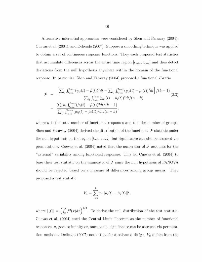
Alternative inferential approaches were considered by Shen and Faraway (2004),

Cuevas et al. (2004), and Delicado (2007). Suppose a smoothing technique was applied

to obtain a set of continuous response functions. They each proposed test statistics

that accumulate differences across the entire time region [tmin, tmax] and thus detect

deviations from the null hypothesis anywhere within the domain of the functional

response. In particular, Shen and Faraway (2004) proposed a functional F -ratio

F =

[∑ij

∫ tmax

tmin(yij(t)− µ(t))2dt−

∑ij

∫ tmax

tmin(yij(t)− µi(t))

2dt]/(k − 1)∑

ij

∫ tmax

tmin(yij(t)− µi(t))2dt/(n− k)

(2.3)

=

∑i ni

∫ tmax

tmin(µi(t)− µ(t))2dt/(k − 1)∑

ij

∫ tmax

tmin(yij(t)− µi(t))2dt/(n− k)

,

where n is the total number of functional responses and k is the number of groups.

Shen and Faraway (2004) derived the distribution of the functional F statistic under

the null hypothesis on the region [tmin, tmax], but significance can also be assessed via

permutations. Cuevas et al. (2004) noted that the numerator of F accounts for the

“external” variability among functional responses. This led Cuevas et al. (2004) to

base their test statistic on the numerator of F since the null hypothesis of FANOVA

should be rejected based on a measure of differences among group means. They

proposed a test statistic

Vn =k∑

i<j

ni||µi(t)− µj(t)||2,

where ||f || =(∫ b

af 2(x)dx

)1/2. To derive the null distribution of the test statistic,

Cuevas et al. (2004) used the Central Limit Theorem as the number of functional

responses, n, goes to infinity or, once again, significance can be assessed via permuta-

tion methods. Delicado (2007) noted that for a balanced design, Vn differs from the

17

numerator of F only by a multiplicative constant. Delicado (2007) also showed equiv-

alence between (3.2) and the Analysis of Distance approach in Gower and Krzanowski

(1999).

The region-wise approach, like in Shen and Faraway (2004) and Cuevas et al.

(2004), performs an overall FANOVA test, i.e., detects a significant difference any-

where in [tmin, tmax]. However, once overall significance is established, one may want

to perform a follow-up test across t to identify specific regions of time where the sig-

nificant difference among functional means has occurred. The point-wise approaches

of Ramsay and Silverman (2005) and Cox and Lee (2008) can be considered as follow-

up tests but both techniques have their caveats. Ramsay and Silverman (2005) fail

to account for the multiplicity issue while performing L tests across the evaluation

points. Cox and Lee (2008) account for multiplicity but their method can not as-

sess overall significance. Using either point-wise approach as a follow-up test could

produce results that are inconsistent with the overall test inference.

The remainder of the paper is organized in the following way. Section 3 discusses

the problem of multiplicity that has been briefly mentioned above. In Section 4

we propose a new method to perform a follow-up test in the FANOVA setting and

contrast it to the existing method of Cox and Lee (2008). Sections 5 and 6 present

simulation study results, Section 7 applies the methods to data from a study of

CO2 impact on spectral measurements of vegetation, and Section 8 concludes with a

discussion.

3. Multiple Testing Procedures

In hypothesis testing problems involving a single null hypothesis, the statistical

tests are chosen to control the Type I error rate of incorrectly rejecting H0 at a

18

prespecified significance level α. If L hypotheses are tested simultaneously, the prob-

ability of at least one Type I error increases in L, and will be close to one for large

L. That is, a researcher will commit a Type I error almost surely and thus wrongly

conclude that results are significant. To avoid these situations with misleading find-

ings, the p-values based on which the decisions are made should be adjusted for L

simultaneous tests.

A common approach to the multiplicity problem calls for controlling the family-

wise error rate (FWER), the probability of committing at least one Type I error.

Statistical procedures that properly control for the FWER, and thus adjust the p-

values based on which a decision is made, are called multiple comparison or multiple

testing procedures. Generally, multiple comparison procedures can be classified as ei-

ther single-step or stepwise. Single-step multiple testing procedures, e.g., Bonferroni,

reject or fail to reject a null hypothesis without taking into account the decision for

any other hypothesis. For stepwise procedures, e.g., Holm (1979), the rejection or

non-rejection of a null hypothesis may depend on the decision of other hypotheses.

Simple single-step and stepwise methods produce adjusted p-values of 1 whenever the

number of tests, L, goes to ∞. Since, in the functional response setting, the possi-

ble number of tests is potentially infinite, one needs to employ more sophisticated

multiplicity adjustment methods. Two possibilities are reviewed below.

The Westfall-Young method (Westfall and Young (1993)) is a step-down re-

sampling method, i.e., the testing begins with the first ordered hypothesis (corre-

sponding to the smallest unadjusted p-value) and stops at the first non-rejection. To

implement this method first find unadjusted p-values and order them from min to

max, p(1) ≤ . . . ≤ p(L). Generate a vector (p∗(1),n, . . . , p∗(L),n), n = 1, . . . , N , from the

same, or at least, approximately the same, distribution as the original p-values under

the global null. That is, randomly permute observations N times. For each permu-

19

tation compute the unadjusted p-values (p∗1,n, . . . , p∗L,n), where n indexes a particular

permutation. Put the p∗l,n’s, l = 1, . . . , L, in the same order as p-values for the original

data. Next, compute successive minima q∗(l),n = min{p∗(s),n : s ≥ l}, l = 1, . . . , L for all

permutations n = 1, . . . N . Finally, the adjusted p-value is the proportion of the q∗(l),n

less than or equal to p(l), with an additional constraint of enforced monotonicity (suc-

cessive ordered adjusted p-values should be greater or equal than one another). See

Westfall and Young (1993) Algorithm 2.8 for a complete description of the method.

Another approach is the closure method, which is based on the union-intersection

test. The union-intersection test was proposed by Roy (1953) as a method of con-

structing a test of any global hypothesis H0 that can be expressed as an inter-

section of the collection of individual (or elementary) hypotheses. If the global

null is rejected, one has to decide which individual hypothesis Hl is false. Mar-

cus et al. (1976) introduced the closure principle as a construction method which

leads to a step-wise test adjustment procedure, and allows one to draw conclusions

about the individual hypotheses. The closure principle can be summarized as fol-

lows. Define a set H = {H1, . . . , HL} of individual hypotheses and the closure set

H = {HJ = ∩j∈JHj : J ⊂ {1, . . . , L}, HJ 6= ∅}. For each intersection hypoth-

esis HJ ∈ H, perform a test and reject individual Hj if all hypotheses HJ ∈ H

with j ∈ J are rejected. For example, if L = 5 then the closure set is H =

{H1, H2, . . . , H5, H12, H13, . . . , H45, H123, H124, . . . , H345, H1234, H1235, . . . , H2345, H12345}.

The entire closure set for L = 5 is shown in Figure 3.2. A rejection of H1 requires re-

jection of all intersection hypotheses that include H1, which are highlighted in Figure

3.2. See Hochberg and Tamhane (1987) for a discussion of closed testing procedures.

In the closure principle, the global null hypothesis is defined as an intersection

of the individual null hypotheses and therefore one would like to base the global

test statistic on a combination of the individual test statistics. The mapping of the

20

H12345

H1234 H1235 H1245 H1345 H2345

H123 H124 H134 H234 H234 H145 H245 H345H125 H135

H12 H13 H23 H14 H24 H34 H15 H25 H35 H45

H1 H2 H3 H4 H5

Figure 2.1: Closure set for five elementary hypotheses H1, . . . , H5 and their intersec-tions. A rejection of all intersection hypotheses highlighted in colors is required toreject H0.

individual test statistics to a global one is obtained via a combining function. Pesarin

(1992) and Basso et al. (2009) state that a suitable combining function should satisfy

the following requirements: (i) it must be continuous in all its arguments, (ii) must

be non-decreasing in its arguments, (iii) must reach its supremum when one of its

arguments rejects the corresponding partial null hypothesis with probability one.

Basso et al. (2009) suggest the following combining functions in the comparison of

means of two groups:

1. The unweighted sum of T -statistics

Tsum =m∑

h=1

Th,

where Th is the standard Student’s t-test statistic.

21

2. A weighted sum of T -statistics

Twsum =m∑

h=1

whTh,

where wh are the weights with∑wh = 1.

3. A sum of signed T squared statistics

TssT 2 =m∑

h=1

sign(Th)T 2h .

Note that the max{F (tl)} in Ramsay et al. (2009) is an extreme case of the weighted

sum combining function with all of the weights equal to zero except one for the largest

observed test statistic. Also, the numerator of the F statistic, defined in (3.2), can

be viewed in the context of an unweighted sum combining function. We employ this

F numerator property in the development of our method.

In the next section we propose a new procedure to perform a follow-up test in the

FANOVA setting based on the ideas of the closure principle and combining functions.

The closure principle will allow us to make a decision for both the overall test, to

detect a difference anywhere in time t, and adjust the p-values for the follow-up test,

to test across t. By using a combining function we will be able to easily find the

value of the test statistic for the overall null based on the values of the individual test

statistics.

4. Follow-Up Testing in FANOVA

There are two ways in which one can perform follow-up testing to identify regions

with significant differences. One possibility, as in Ramsay and Silverman (2005) and

22

Cox and Lee (2008), is to evaluate the functional responses on a finite, equally spaced

grid of L points from tmin to tmax (see Figure 2.2a). Another possibility, proposed

here, is to split the domain into L mutually exclusive and exhaustive subintervals, say

[al, bl] , l = 1, . . . , L (see Figure 2.2b). Based on these two possibilities, we considered

follow-up tests for the following four possibilities:

-0.2

-0.1

0.0

0.1

0.2

0.3

0.0 0.2 0.4 0.6 0.8 1.0Time

Value

Group

1

2

3

(a)

-0.2

-0.1

0.0

0.1

0.2

0.3

0.0 0.2 0.4 0.6 0.8 1.0Time

Value

Group

1

2

3

(b)

Figure 2.2: Two follow-up testing methods illustrated on simulated data with threegroups, five curves per group, and five evaluation points or regions.

1. The procedure proposed by Cox and Lee (2008), which is to evaluate continuous

functional responses on a finite grid of points, and at each evaluation point

tl, l = 1, . . . , L, perform a parametric F -test. The individual p-values are

adjusted using the Westfall-Young method. We do not consider the Ramsay

and Silverman (2005) procedure because it fails to adjust for L simultaneous

tests.

2. We propose performing a test based on subintervals of the functional response

domain and use the closure principle to adjust for multiplicity. The method

23

is implemented as follows. Apply a smoothing technique to obtain continuous

functional responses. Split the domain of functional responses into L mutually

exclusive and exhaustive intervals such that [tmin, tmax] = ∪Ll=1[al, bl]. Let the

elementary null hypothesis Hl be of no significant difference among functional

means anywhere in t on the subinterval [al, bl]. For each subinterval, find the

individual test statistic Tl as a numerator of F in Equation (3.2)

Tl =

∫ bl

al

ni(µi(t)− µ(t))2dt/(k − 1).

Because significance is assessed using permutations, only the numerator of F

is required to perform the tests. The other reason for this preference is the

fact that the numerator of F nicely fits with the idea of the unweighted sum

combining function. That is

L∑l=1

Tl =L∑l=1

∫[al,bl]

k∑i=1

ni(µj(t)− µ(t))2dt/(k − 1)

=

∫ tmax

tmin

k∑i=1

ni(µi(t)− µ(t))2dt/(k − 1)

= T.

Thus, to test the intersection of two elementary hypotheses, sayHl andHl′ , of no

difference in groups over [al, bl]∪[al′ , bl′ ], construct the test statistic T(ll′) as a sum

of Tl +Tl′ and find the p-value via permutations. The number of permutations,

B, should be chosen such that (B+1)α is an integer to insure that the test is not

liberal (Boos and Zhang (2000)). The p-values of the individual hypotheses Hl

are adjusted according to the closure principle by taking the maximum p-value

24

of all hypotheses in the closure set involving Hl. Intermediate intersections of

hypotheses are adjusted similarly.

3. We also considered performing the test based on the subregions of the func-

tional domain with the Westfall-Young multiplicity adjustment. To imple-

ment the method, first find the unadjusted p-values for each subregion [al, bl],

l = 1, . . . , L, by computing F∗lb for b = 1, . . . , B permutations and then counting

(# of (F∗lb ≥ Fl0))/B, where Fl0 is the value of F for a given sample on the

interval [al, bl]. Then correct the unadjusted p-values using the Westfall-Young

method. Note that to obtain a vector (p∗(1),n, . . . , p∗(L),n), n = 1, . . . , N , the values

(F∗(1),n, . . . ,F∗(L),n) can be computed based on a single permutation and then

compared to the distribution of F∗lb , b = 1, . . . , B, and l = 1, . . . , L, obtained

previously. Thus, instead of simulating L separate permutation distributions

of F∗(l),n’s for each n = 1, . . . , N in the Westfall-Young algorithm, one can use

the same permutation distribution that was generated to calculate the unad-

justed p-values. This dual use of one set of permutations dramatically reduces

the computational burden of this method without impacting the adjustment

procedure.

4. Finally, we considered a combination of the point-wise test with the closure

method for multiplicity adjustment. The procedure is implemented as follows.

First, evaluate functional responses on a grid of L equally spaced points and

obtain individual test statistics at each of L evaluation points based on the

regular univariate F -ratio. Then calculate the unadjusted p-values based on

B permutations and use the unweighted sum combining function to obtain the

global test statistic and all of the test statistics for the hypotheses in the closure

set. In other words, to obtain a test statistic for the overall null hypothesis of

25

no difference anywhere in t simply calculate∑L

l=1 Fl. Note that this combining

method is equivalent to the sum of signed T -squared statistics, TssT 2 , suggested

by Basso et al. (2009). The adjusted p-values of the elementary hypothesis Hl

are once again found by taking the maximum p-value of all hypotheses in the

closure set involving Hl.

5. Simulation Study

Now, we present a small simulation study to examine properties of the point-wise

follow-up test proposed by Cox and Lee (2008), the region-based method with the

closure adjustment, the region-based method with the Westfall-Young adjustment,

and the point-wise test with the closure adjustment. The properties of interest were

the weak control of the FWER, the strong control of the FWER, and power. Hochberg

and Tamhane (1987) define the error control as weak if the Type I error rate is

controlled only under the global null hypothesis, H = ∩mk=1Hk, which assumes that all

elementary null hypotheses are true. Hochberg and Tamhane (1987) define the error

control as strong if the Type I error rate is controlled under any partial configurations

of true and false null hypotheses. To study the weak control of the FWER, we

followed the setup of Cuevas et al. (2004) and simulated 25 points from yij(t) =

t(1 − t) + εij(t) for i = 1, 2, 3, j = 1, . . . , 5, t ∈ [0, 1], and εij ∼ N(0, 0.152). Once

the points were generated, we fit these data with smoothing cubic B-splines, with 25

equally spaced knots at times t1 = 0, . . . , t25 = 1. A smoothing parameter, λ, was

selected by generalized cross-validation. To study the strong control of the FWER, the

observations for the third group were simulated as y3j(t) = t(1−t)+0.05beta(37,37)(t)+

ε3j(t), where betaa,b(t) is the density of the Beta(a, b) distribution. In our simulation

study, this setup implied a higher proportion of Ha’s in the partial configuration of

26

true and false hypotheses as the number of tests increased. To investigate the power,

we considered a shift alternative, where the observations for the third group were

simulated as y3j(t) = t(1− t) + δ + ε3j(t) and δ = 0.03, 0.06, 0.09, and 0.12. We also

wanted to check whether the two methods are somewhat independent of the number

of evaluation points or evaluation intervals. To check this condition, we performed

follow-up testing at either m = 5 or m = 10 intervals/evaluation points.

For this study, we needed two simulation loops. The outside loop was of size

O = 1000 replications. For each iteration, the permutation-based p-values for the

point-wise method with the Westfall-Young adjustment were calculated using the

mt.minP function from the multtest R package (Pollard et al. (2011)). We would

like to point out that, unlike the suggestion in Cox and Lee (2008) to use a para-

metric F distribution to find the unadjusted p-values, the mt.minP function finds the

unadjusted p-values via permutations. For the region-based method with the closure

adjustment, the unadjusted p-values were calculated using the adonis function from

the vegan package (Oksanen et al. (2011)). We wrote an R script to adjust the p-

values according to the closure principle. The calculation of the p-values based on

the region method with the Westfall-Young adjustment required computation of m

unadjusted p-values based on B = 999 permutations and a consecutive simulation of

N vectors (p∗(1),n, . . . , p∗(m),n), n = 1, . . . , N . To reduce computation time during power

investigation for the third scenario, we used a method of power extrapolation based

on linear regression described by Boos and Zhang (2000). The method is implemented

by first finding three 1 ×m vectors of the adjusted p-values based on the Westfall-

Young algorithm for (N1, N2, N3) = (59, 39, 19) for each iteration of the outside loop.

27

Method 5 intervals/evaluations 10 intervals/evaluations

Region-based/Closure 0.020± 0.009 0.008± 0.006Point-wise/Closure 0.028± 0.010 0.008± 0.006Region-based/Westfall-Young 0.043± 0.013 0.034± 0.011Point-wise/Westfall-Young 0.045± 0.013 0.045± 0.013

Table 2.1: Estimates of the Type I error (± margin of error) control in the weak sensefor α = 0.05.

Then the estimated power is computed at each subregion as

powk,Nr=

1

O

O∑j=1

I(pk,Nr ≤ α),

where I() is an indicator function, r = 1, 2, 3, k = 1, . . . ,m, O = 1000, and pk is

the adjusted p-value for the kth subregion based on the Westfall-Young algorithm.

Finally, the adjusted power based on the linear extrapolation was calculated as

powk,lin = 1.01137(powk,59) + 0.61294(powk,39)− 0.62430(powk,19).

The p-values for the point-wise test with the closure adjustment were also found

based on B = 999 inner permutations. For all scenarios an R script is available upon

request.

6. Simulation Results

Tables 2.1 and 2.2 report estimates of the family-wise error rate in the weak and

the strong sense respectively for the nominal significance level of 5%. The margin

of errors from 95% confidence intervals have been calculated based on the normal

approximation of the binomial distribution.

28

Method 5 intervals/evaluations 10 intervals/evaluations

Region-based/Closure 0.042± 0.012 0.035± 0.011Point-wise/Closure 0.047± 0.013 0.049± 0.013Region-based/Westfall-Young 0.050± 0.014 0.111± 0.019Point-wise/Westfall-Young 0.039± 0.012 0.071± 0.016

Table 2.2: Estimates of the Type I error (± margin of error) control in the strongsense for alpha = 0.05.

Table 2.1 indicates that both testing methods tend to be conservative whenever

the closure multiplicity adjustment is applied with the simulations under the global

null (highlighted in bold). From Table 2.2 it is evident that both testing methods

with the Westfall-Young multiplicity adjustment become liberal as the proportion of

Ha’s increases in the configuration of the true and false null hypotheses (highlighted in

bold). We offer the following explanation for this phenomenon. The test for the overall

significance, i.e., whether or not a difference in mean functions exists anywhere in t, is

not always rejected if the observations are coming from a mixture of the hypotheses.

The closure principle rejects an individual hypothesis only if all hypotheses implied by

it (including the overall null) are rejected. Thus, whenever the overall null is accepted,

the individual p-values are adjusted accordingly – over the level of significance – and

control of the FWER in the strong sense is maintained. With the Westfall-Young

method the overall test is not performed. Only the individual p-values are penalized

for multiplicity, but the penalty is not “large” enough which likely causes the method

to be liberal.

The results of the power investigation for 5 intervals/evaluation points are illus-

trated in Figure 2.3 and for 10 intervals/evaluation points in Figure 2.4. Solid lines

correspond to power of the region-based method with the closure adjustment, dashed

lines to the region-based method with the Westfall-Young adjustment, solid circles

29

to the point-wise test with the Westfall-Young adjustment, and solid triangles to the

point-wise method with the closure adjustment. The grouping of power results based

on the shift amount, δ, is pretty apparent but a transparency effect is added to aid

visualization. The most solid objects (lower graph) correspond to a shift of δ = 0.03,

and the most transparent objects (upper graph) to δ = 0.12.

From Figure 2.3 it appears that a combination of the closure multiplicity correction

with either testing method provides higher power across all testing points/intervals

for moderate values of the shift deviation (δ = 0.06 and δ = 0.09) than the Wetsfall-

Young method. There does not seem to be any striking visual difference in power of

the four methods for the lowest and highest shift amount (δ = 0.03 and δ = 0.12).

Although the powers were very close at the extreme values of δ, it appears that the

closure multiplicity correction provides higher overall power across different values of

δ while maintaining its conservative nature under the global null. Similar conclusions

can be drawn based on Figure 2.4.

A contrast of Figure 2.4 to Figure 2.3 reveals that all methods tend to lose power

as the number of evaluation points/intervals increases. This observation implies an

intuitive result that a region-based method should be more powerful than a point-

wise method. That is, in a real application of a point-wise method one would want to

employ many more than m = 10 evaluation points. With the region-based application

one may not have more than a few a priori specified subintervals of interest. Since

the power of methods decreases with an increase in m, a region-wise method with a

modest number of intervals provides a higher-powered alternative to the point-wise

procedures, as they would be used. Additional simulation results for larger values of

m provided in the supplementary material support this conclusion.

Both Figures 2.3 and 2.4 indicate that a point-wise test in a combination with the

closure procedure provides the highest power. However, there is a caveat in a potential

30

application of this method. The cardinality of the closure set with m testing points

is 2m − 1. Therefore, if one would like to perform point-wise tests on a dense grid

of evaluation points, the closure principle might become impractical. For example,

if one wants to perform a test at m = 15 points, |H| = 32, 767, where |H| denotes

the cardinality of the closure set H. Zaykin et al. (2002) proposed a computationally

feasible method for isolation of individual significance through the closure principle

even for a large number of tests. However, since in our application the region-based

follow-up test directly addresses research questions and the number of elementary hy-

potheses is typically small, we left an implementation of this computational shortcut

for future study.

As mentioned above, the closure multiplicity correction provides an additional

advantage over the Westfall-Young correction of being able to assess the overall signifi-

cance. Cox and Lee (2008) suggest taking a leap of faith that when the Westfall-Young

corrected p-values are below the chosen level of significance, then there is evidence

of overall statistical significance. A use of any combining method along with the

closure principle allows one to perform a global test as well as to obtain multiplicity

adjusted individual p-values. The closure method also provides adjusted p-values for

all combinations of elementary hypotheses and the union of some sub-intervals may

be of direct interest to researchers.

7. Application

Data from an experiment related to the effect of leaked carbon dioxide (CO2) on

vegetation stress conducted at the Montana State University Zero Emissions Research

and Technology (ZERT) site in Bozeman, MT are used to motivate these methods.

Further details may be found in Bellante et al. (2013). One of the goals of the

31

Time

Pow

er

0.2

0.4

0.6

0.8

0.0 0.2 0.4 0.6 0.8 1.0

Follow-up Method

Region-based/Closure

Point-wise/Closure

Region-based/Westfall-Young

Point-wise/Westfall-Young

Figure 2.3: Power of the four methods at different values of the shift amount. Thesolid objects in the lower graph correspond to δ = 0.03. The three groups of objectsabove that correspond to δ = 0.06, 0.09, and 0.12 respectively.

Time

Pow

er

0.2

0.4

0.6

0.8

0.0 0.2 0.4 0.6 0.8 1.0

Follow-up Method

Region-based/Closure

Point-wise/Closure

Region-based/Westfall-Young

Point-wise/Westfall-Young

Figure 2.4: Power of the four methods with 10 intervals/evaluation points.

32

experiment was to investigate hyperspectral remote sensing for monitoring geologic

sequestration of carbon dioxide. A safe geologic carbon sequestration technique must

effectively store large amounts of CO2 with minimal surface leaks. Where vegetation is

the predominant land cover over geologic carbon sequestration sites, remote sensing is

proposed to indirectly identify subsurface CO2 leaks through detection of plant stress

caused by elevated soil CO2. During the course of the month long controlled CO2

release experiment, an aerial imaging campaign was conducted with a hyperspectral

imager mounted to a small aircraft. A time series of images was generated over the

shallow CO2 release site to quantify and characterize the spectral changes in overlying

vegetation in response to elevated soil CO2.

We analyzed measurements acquired on June 21, 2010 during the aerial imaging

campaign over the ZERT site. The pixel-level measurements consisted of 80 spectral

reflectance responses between 424.46 and 929.27 nm. For each pixel, we calculated

the horizontal distance of the pixel to the CO2 release pipe. We hypothesized that

the effect of the CO2 leak on plant stress would diminish as we moved further away

from the pipe. To test this, we binned the continuous measurements of distance into

five subcategories: (0,1], (1,2], (2,3], (3,4], and (4,5] meters to the CO2 release pipe.

Our null hypothesis was that the spectral responses obtained at different distances

are indistinguishable. Thus, we could assume exchangeability and permute observa-

tions across distances under the null hypothesis. Since the entire image consisted of

over 30,000 pixels, we randomly selected 500 pixels from each of the binned distance

groups. The spectral responses in 80 discrete wavelengths were generally smooth,

providing an easy translation to functional data. There were 2500 spectral response

curves in total, with a balanced design of a sample of 500 curves per binned dis-

tance. Overall significance was detected (permutation p-value=0.0003), so we were

interested in identifying the regions of the electromagnetic spectrum where the sig-

33

nificant differences occurred. In particular, we were interested in whether there were

significant differences in the visible (about 400 nm to 700 nm), “red edge” (about

700 nm to 750 nm), and near infrared (about 750 nm to 900 nm) portions of the

electromagnetic spectrum. Since our spectral response ranged to 929.27 nm, we also

included the additional region of >900 nm. Because of our interest in specific regions

of the electromagnetic spectrum, the regionalized analysis of variance based on the F

test statistic was performed for each of the four spectral regions. The corresponding

unadjusted p-values were found based on the permutation approximation. For each

region we applied the two multiplicity correction methods, namely the closure and

the Westfall-Young method. The results are shown in Figure 4.6.

The p-values adjusted by the two methods are quite similar to each other. Both

methods returned the lowest p-value corresponding to the “red edge” spectral region.

This is a somewhat expected result since the “red edge” spectral region is typically

associated with plant stress. In addition, significant differences were detected in

both the visible and near infrared regions. The observed difference between the two

adjustments is probably due to the fact that the p-values adjusted with the closure

method cannot be lower than the overall p-value, while the Westfall-Young method

does not have this restriction. These results demonstrate the novelty and utility of our

approach with regards to this application. A previous attempt at examining spectral

responses as a function of distance to the CO2 release pipe relied on a single spectral

index as opposed to the full spectral function (Bellante et al. (2013)). Identification of

significant differences among spectral regions could prove to be an important analysis

technique for hyperspectral monitoring of geologic carbon sequestration. By using a

method that provides strong Type I error control, we can reduce false detection of

plant stress which could lead to unneeded and costly examination of CO2 sequestra-

tion equipment in future applications of these methods.

34

Mean Spectral Curves

Wavelength (nm)

Pixel

Rad

iance

5000

10000

15000

p-valueWY =0.002

p-valueWY=0.002

p-valueWY=0.016

p-valueWY=0.066

p-valueCl=0.009

p-valueCl=0.003

p-valueCl=0.009

p-valueCl=0.057

Visible Light

Red Edge

Near Infrared

>900 nm

500 600 700 800 900

Distance to the Pipe (m)

(0,1]

(1,2]

(2,3]

(3,4]

(4,5]

Figure 2.5: Plot of mean spectral curves at each of the five binned distances tothe CO2 release pipe. p-valueWY represents a p-value obtained by a combinationof the regionalized testing method with the Westfall-Young multiplicity correction.p-valueCL represents a p-value obtained by the regionalized method with the closuremultiplicity adjustment.

8. Discussion

We have suggested an alternative procedure to the method proposed by Cox and

Lee (2008) to perform follow-up testing in the functional analysis of variance setting.

Although there is no single approach that is superior in every situation, we have shown

in our simulation study that the method for the individual p-value adjustment based

35

on combining functions via the closure principle provides higher power than that based

on the Westfall-Young adjustment. We have shown that the multiplicity adjustment

method based on the closure principle tends to be conservative assuming a common

mean function, µ(t), for all t (i.e., on the entire functional domain). The Westfall-

Young method was shown to be liberal assuming heterogeneous mean functions, µi(t),

on some subregions of the functional domain.

The point-wise follow-up testing method provides slightly higher power than the

region-based method. However, we would like to stress one more time that these two

methods should not be considered as direct competitors. The choice of one follow-up

testing method over the other should be application driven. In our application, we

were interested in significant differences in regions of the electromagnetic spectrum

and applied the region-based method. In this case it showed similar results with the

two multiplicity adjustment corrections despite their differences in performance in

simulations.

36

References


Bellante, J., Powell, S., Lawrence, R., Repasky, K., Dougher, T., 2013. Aerial detec-tion of a simulated co2 leak from a geologic sequestration site using hyperspectralimagery. International Journal of Greenhouse Gas Control 13, 124–137.

Boos, D. D., Zhang, J., 2000. Monte carlo evaluation of resampling-based hypothesistests. Journal of the American Statistical Association 95, 486–492.



Delicado, P., 2007. Functional k-sample problem when data are density functions.Computational Statistics 22 (3), 391–410.

Gower, J. C., Krzanowski, W. J., 1999. Analysis of distance for structured multivari-ate data and extensions to multivariate analysis of variance. Journal of the RoyalStatistical Society 48 (4), 505–519.

Hochberg, Y., Tamhane, A. C., 1987. Multiple Comparison Procedures. Wiley.

Holm, S., 1979. A simple sequentially rejective multiple test procedure. ScandinavianJournal of Statistics 6, 65–70.


Oksanen, J., Blanchet, F. G., Kindt, R., Legendre, P., Minchin, P. R., O’Hara,R. B., Simpson, G. L., Solymos, P., Stevens, M. H. H., Wagner, H., 2011. vegan:Community Ecology Package. R package version 2.0-1.URL http://CRAN.R-project.org/package=vegan


Pollard, K. S., Gilbert, H. N., Ge, Y., Taylor, S., Dudoit, S., 2011. multtest:Resampling-based multiple hypothesis testing. R package version 2.10.0.

http://CRAN.R-project.org/package=vegan

37


Ramsay, J. O., Hooker, G., Graves, S., 2009. Functional Data Analysis with R andMATLAB. Springer.


Ramsay, J. O., Wickham, H., Graves, S., Hooker, G., 2012. fda: Functional DataAnalysis. R package version 2.3.2.URL http://CRAN.R-project.org/package=fda

Roy, S. N., 1953. On a heuristic method of test construction and its use in multivariateanalysis. The Annals of Mathematical Statistics 23 (220-238).

Shen, Q., Faraway, J., 2004. An F test for linear models with functional responses.Statistica Sinica 14, 1239–1257.

Westfall, P. H., Young, S. S., 1993. Resampling-based Multiple Testing: Examplesand Methods for P-Value Adjustment. Wiley.

Zaykin, D. V., Zhivotovsky, L. A., Westfall, P. H., Weir, B. S., 2002. Truncatedproduct method for combining p-values. Genetic Epidemiology 22 (2), 170–185.


http://CRAN.R-project.org/package=fda

38

CHAPTER 3

PAIRSWISE COMPARISON OF TREATMENT LEVELS IN FUNCTIONAL

ANALYSIS OF VARIANCE WITH APPLICATION TO ERYTHROCYTE

HEMOLYSIS.



Contributions: Wrote the majority of the manuscript.



Co-Author: Dmitri Holodov

Contributions: Collected the data. Provided field expertise.

39


Olga A. Vsevolozhskaya, Mark C. Greenwood, Dmitri Holodov

Journal of Annals of Applied Statistics.


Prepared for submission to a peer-reviewed journal

X Officially submitted to a peer-review journal

Accepted by a peer-reviewed journal


Published by Institute of Mathematical Statistics.

Submitted April, 2013

40

Abstract

Motivated by a practical need for the comparison of hemolysis curves at varioustreatment levels, we propose a novel method for pairwise comparison of mean func-tional responses. The hemolysis curves – the percent hemolysis as a function of time –of mice erythrocytes (red blood cells) by hydrochloric acid have been measured amongdifferent treatment levels. This data set fits well within the functional data analysisparadigm, in which a time series is considered as a realization of the underlyingstochastic process or a smooth curve. Previous research has only provided methodsfor identifying some differences in mean curves at different times. We propose atwo-level follow-up testing framework to allow comparisons of pairs of treatmentswithin regions of time where some difference among curves is identified. The closuremultiplicity adjustment method is used to control the family-wise error rate of theproposed procedure.

1. Introduction

The use of non-steroidal anti-inflammatory drugs (NSAIDs) is wide-spread in the

treatment of various rheumatic conditions (Nasonov and Karateev (2006)). Gastroin-

testinal symptoms are the most common adverse events associated with the NSAID

therapy (Garcia-Rodriguez et al. (2001)). Holodov and Nikolaevski (2012) suggested

oral administration of procaine (novocaine) solution in low concentration (0.25 to 1%)

to reduce the risk of upper gastrointestinal ulcer bleeding associated with NSAIDs.

To validate the effectiveness of the proposed therapy, an experiment was conducted

to study the effect of novocaine on the resistance of the red blood cells (erythrocytes)

to hemolysis by hydrochloric acid. Hydrochloric acid is a major component of gastric

juice and a lower rate of erythrocyte hemolysis should indicate a protective effect of

novocaine.

Hemolytic stability of erythrocytes for the control and three different dosages of

novocaine (4.9× 10−6 mol/L, 1.0× 10−5mol/L, and 2.01× 10−5mol/L) was measured

as a percentage of hemolysed cells. The data for the analysis were curves of hemolysis

41

(erythrograms) that were measured as functions of time. Figure 3.1 illustrates a sam-

ple of percent hemolysis curves. The goal of the statistical analysis was to summarize

the associated evidence across time of the novocaine effect including performing pair-

wise comparisons of novocaine dosages.

0

20

40

60

80

0 200 400 600Time (sec)

Hem

olys

is %

Novocaine Dosage

control

low

medium

high

Figure 3.1: Hemolysis curves of mice erythrocytes by hydrochloric acid with super-imposed estimated mean functions.

Most current approaches essentially evaluate differences among groups of curves

point-wise (typically, with many one-way ANOVA tests). For such approaches, when

testing is performed at a large number of points simultaneously, the type I error rate is

going to be inflated. Cox and Lee (2008) proposed a method that utilizes a point-wise

approach, while properly controlling Type I error, and can be used for investigating

specific subregions of the functional domain (time) for a significant difference. Alter-

natively, the functional analysis of variance (FANOVA) can be employed to perform

testing among k groups of curves. The overall functional testing methods, such as the

functional F of Shen and Faraway (2004) or the functional Vn of Cuevas et al. (2004),

42

can be utilized to test for associated evidence across the entire functional domain

(across all time). However, none of these methods allow for pairwise comparisons of

functional means. Thus, the challenge for the current analysis was to determine dif-

ferences among novocaine dosages withing specific intervals of time, where significant

difference among hemolysis curves is present.

In this paper, we introduce a new two-step procedure: first, to detect regions in

time of “significant” differences among mean curves, and second, to perform a pair-

wise comparison of treatment levels within those regions. Our approach utilizes two

ideas: (i) combining methods to map the test statistics of the individual hypotheses,

H1, . . . , Hm, to the global one, ∩mi=1Hi, and (ii) the closure principle of Marcus et al.

(1976) to control the family-wise error rate (FWER), the probability of at least one

false rejection. The rest of the article is organized in the following manner. We give

an overview of the FANOVA problem and the existing methods for investigating the

functional domain for significant differences. We discuss the proposed procedure for

investigating regions of time for significant differences and detail a computational

shortcut that allows isolation of individual significance even for a large number of

tests. We extend the proposed procedure to perform pairwise comparisons of the

treatment levels within identified functional regions of statistical significance. The

protective effect of novocaine is demonstrated based on the different patterns between

groups detected in certain regions of time.

2. Methods

Functional analysis of variance involves testing for some difference among k func-

tional means. In functional data analysis, t is used to denote a real-valued variable

(usually of time), and y(t) denotes a continuous outcome, which is a function of t.

43

Then, the FANOVA model is written as:

yij(t) = µi(t) + εij(t), (3.1)

where µi(t) is the mean function of group i at time t, i = 1, . . . , k, j indexes a

functional response within a group, j = 1, . . . , ni, and εij(t) is the residual function.

Each εij(t) is assumed to be a mean zero and independent Gaussian stochastic process.

The FANOVA hypotheses are written as:

H0 : µ1(t) = µ2(t) = . . . = µk(t)


The alternative hypothesis considers any difference anywhere in t among k population

means of yij(t).

In recent years two different general approaches have emerged to perform the

FANOVA test. In Shen and Faraway (2004), as well as many other papers (see

Cuevas et al. (2004), Ramsay et al. (2009) and Cuesta-Albertos and Febrero-Bande

(2010)), a global test statistic has been developed to perform the FANOVA test. The

statistic is “global” because it is used to detect differences anywhere in the entire

functional domain (anywhere in t). An alternative approach (Ramsay and Silverman

(2005) and Cox and Lee (2008)) is to use a point-wise (or individual) test statistic to

perform inference across t, i.e., identify specific regions of t with significant difference

among functional means.

44

2.1. “Global” Approach

Suppose the domain [a, b] of functional responses can be split into m pre-specified

mutually exclusive and exhaustive intervals such that [a, b] = ∪mi=1 [ai, bi]. For in-

stance, in the novocaine experiment the researchers were interested in the effect of

novocaine during specific time intervals associated with hemolysis of different ery-

throcyte populations: hemolysis of the least stable population ([a2, b2] = 61-165 sec.),

general population ([a3, b3] = 166-240 sec.), and most stable ([a4, b4] = over 240 sec.).

For each interval [ai, bi], i = 1, . . . ,m, an individual functional statistic of Shen and

Faraway (2004), Fi, i = 1, . . .m, can be calculated as

Fi =

∫[ai,bi]

∑kj=1 nj(µj(t)− µ(t))2dt/(k − 1)∫

[ai,bi]

∑kj=1

∑ns=1(yjs(t)− µj(t))2dt/(n− k)

, (3.2)

where n is the total number of functional responses and k is the number of groups.

The numerator of the F statistic accounts for “external” variability among func-

tional responses and the denominator for the “internal” variability. Cuevas et al.

(2004) argues that the null hypothesis should be rejected based on the measure of the

differences among groups, i.e., the “external” variability. Hence, Cuevas et al. (2004)

proposed a statistic Vn based on the numerator of F :

Vn =k∑

i<j

ni||µi(t)− µj(t)||2, (3.3)

where || · || is the L2 norm. Gower and Krzanowski (1999) also argue that in a

permutation setting a test can be based just on the numerator of the test statistic.

That is, if only the numerator of the functional F is used, the changes to the test

statistic are monotonic across all permutations and thus probabilities obtained are

45

identical to the ones obtained from the original F . Additionally, Delicado (2007)

points out that for a balanced design, the numerator of the functional F and Vn differ

by only a multiplicative constant.

2.2. Point-wise Approach

Suppose that a set of smooth functional responses is evaluated on a dense grid of

points, t1, . . . , tm. For instance, the percentage of hemolysed cells can be evaluated

every second. Cox and Lee (2008) propose a test for differences in the mean curves

from several populations, i.e., perform functional analysis of variance, based on these

discretized functional responses. First, at each of the m evaluation points, the regular

one-way analysis of variance test statistic, Fi, i = 1, . . . ,m, is computed. For each

test the p-value is calculated based on the parametric F -distribution and then the

Westfall-Young randomization method (Westfall and Young (1993)) is applied to

correct the p-values for multiplicity. The implementation of the method can be found

in the multtest (Pollard et al. (2011)) R package (R Core Team (2013)).

Certain criticisms may be raised for both the “global” and the point-wise ap-

proaches. First, the point-wise approach can determine regions of the functional

domain with a difference in the means, but can not determine which pairs of pop-

ulations are different. Second, for the Cox and Lee (2008) procedure, the p-value

for the global test can not be obtained, which is an undesirable property since the

method might be incoherent between the global and point-wise inference. We suggest

a procedure that overcomes both of these issues. By using a combining function along

with the closure principle of Marcus et al. (1976) we are able to obtain the p-value for

the overall test as well as adjust the individual p-values for multiplicity. This method

also allows us to perform a pairwise comparison of the group’s functional means and

therefore determine which populations are different in each region.

46

2.3. Proposed Methodology

Once again, suppose the domain [a, b] is split into m pre-specified mutually exclu-

sive and exhaustive intervals. We propose to use the numerator of the functional F as

the test statistic Ti, i = 1, . . . ,m, for each [ai, bi], and then utilize a combining function

to obtain the test statistic for the entire [a, b]. Typical combining functions have the

same general form: the global statistic is defined as a weighted sum, T =∑wiTi,

of the individual statistics with some wi weights (see Pesarin (1992) and Basso et al.

(2009)). A p-value for the overall null hypothesis (that all individual null hypotheses

are true) is based either on the distribution of the resulting global statistic T or on a

permutation approximation. If the unweighted sum combining function is applied to

the proposed Ti, then

T =

∫[a,b]

k∑j=1

nj(µj(t)− µ(t))2dt/(k − 1)

=m∑i=1

∫[ai,bi]

k∑j=1

nj(µj(t)− µ(t))2dt/(k − 1)

=m∑i=1

Ti.

The closure procedure is then applied to perform the overall test based on this com-

bining functions as well as adjust the individual p-values for multiplicity. The closure

method is based on testing all nonempty intersections of the set of m individual hy-

potheses, which together form a closure set. The procedure rejects a given hypothesis

if all intersections of hypotheses that contain it as a component are rejected. Hochberg

and Tamhane (1987) show that the closure procedure controls the family-wise error

47

rate (FWER) at a strong level, meaning that the type I error is controlled under any

partial configuration of true and false null hypotheses.

When the number of individual tests m is relatively large, the use of the closure

method becomes computationally challenging. For example, setting m = 15 results in

215−1 = 32, 767 intersections of hypotheses. Hochberg and Tamhane (1987) described

a shortcut for the T = max{Ti} combining function, where Ti stands for the ith test

statistic for i in the set of Hi pertinent to a particular intersection hypothesis. For

this combining function they showed that the significance for any given hypothesis in

the closure set can be determined using only m individual tests. Zaykin et al. (2002)

described a shortcut for the closure principle in the application of their truncated

p-value method (TPM) that uses an unweighted sum combining function. In the next

section we exploit the shortcut described by Zaykin et al. (2002) and show that for

the T =∑Ti combining function the required number of evaluations is m(m+ 1)/2.

2.3.1. The Shortcut Version of the Closure Procedure The shortcut version of

the closure method for the unweighted sum combining function should be imple-

mented as follows. First, order the individual test statistics from minimum to maxi-

mum as T(1) ≤ T(2) ≤ . . . ≤ T(m), where

Ti =

∫[ai,bi]

k∑j=1

nj(µj(t)− µ(t))2dt/(k − 1). (3.4)

Let H(1), H(2), . . . , H(m) be the corresponding ordered individual hypotheses of no

significant difference among functional means on the interval[a(i), b(i)

], i = 1, . . . ,m.

Now, among intersection hypotheses of size two:

T(1) + T(2) ≤ T(1) + T(3) ≤ . . . ≤ T(1) + T(m),

48

T(2) + T(3) ≤ T(2) + T(4) ≤ . . . ≤ T(2) + T(m),

. . .

Here, the statistic T(i) +T(j) corresponds to intersection hypotheses H(ij) of no signif-

icant difference on both intervals[a(i), b(i)

]∪[a(j), b(j)

]. Among intersections of size

three:

T(1) + T(2) + T(3) ≤ T(1) + T(2) + T(4) ≤ . . . ≤ T(1) + T(2) + T(m),

T(2) + T(3) + T(4) ≤ T(2) + T(3) + T(5) ≤ . . . ≤ T(2) + T(3) + T(m),

. . .

Thus, significance for the hypothesis H(m) can be determined by looking for the largest

p-value among m tests

T(m), T(m) + T(1), . . . ,m∑i=1

T(i).

For the hypothesis H(m−1), the significance can be determined by investigating the

p-values corresponding to (m− 1) tests

T(m−1), T(m−1) + T(1), . . . ,

m−1∑i=1

T(i)

along with the p-value for the test∑m

i=1 T(i) which is already found. Finally, for the

first ordered hypothesis H(1), the significance can be determined by evaluating a single

test T(1) and then looking for the largest p-value among it and the p-values of the

hypotheses H(12), H(123), . . . , H(12...m), which are already evaluated. Thus, significance

of any individual hypothesis H(i) is determined using m p-values, but the number of

unique evaluations to consider is m+ (m− 1) + · · ·+ 1 = m(m+ 1)/2.

49

The described shortcut assumes that all distributions corresponding to the test

statistics are the same and the magnitude of the test statistic has a monotonic rela-

tionship with its p-value. If the p-values for the individual tests are determined from

permutational distributions (as in our situation), a bias will be introduced. The bias

is caused by a mismatch between the minimum value of the test statistics and the

maximum p-value. That is, the minimum statistic is not guaranteed to correspond to

the maximum p-value. The procedure becomes liberal since the individual p-values are

not always adjusted adequately. To reduce and possibly eliminate the bias, we made

the following adjustment to the shortcut. First, we adjusted the individual p-values

according to the shortcut protocol described above and obtained a set of adjusted

individual p-values, p1, p2, . . . , pm. Then, we ordered the individual test statistics

based on the ordering of the unadjusted individual p-values. That is, we order the

unadjusted p-values from maximum to minimum and get a corresponding ordering of

the test statistics T ∗(1), T∗(2) . . . , T

∗(m). Now the inequality T ∗(1) ≤ T ∗(2) ≤ . . . ≤ T ∗(m) will

not necessarily hold. We applied the shortcut based on this new ordering and ob-

tained another set of adjusted individual p-values, p∗1, p∗2, . . . , p

∗m. Finally, the adjusted

individual p-values were computed as max{pi, p∗i }, i = 1, . . . ,m. This correction to

the shortcut increases the number of the required computations by a factor of two,

however it is still of the order m2 instead of 2m.

A small simulation study was used to check whether this version of the correction

provides results comparable to adjustments generated by the entire set of intersection

hypotheses. For the four multiplicity adjustment schemes: (i) correction based on

the ordered test statistics shortcut, (ii) correction based on the ordered unadjusted p-

values shortcut, (iii) correction based on max{pi, p∗i } (combination of both corrections

(i) and (ii)), and (iv) the full closure method, we obtained p-values under the global

null based on 1000 permutations, m = 5, and conducted 1000 simulations, providing

50

5000 corrected p-values. First, we were interested in how many times the p-values

adjusted by various shortcuts were “underestimated” (not corrected enough) relative

to the full closure method. The p-values adjusted by a shortcut based on the ordered

test statistics, p1, p2, . . . , pm, were underestimated 554 out of 5000 times. The p-values

adjusted by a shortcut based on the ordered unadjusted p-values, p∗1, p∗2, . . . , p

∗m, were

underestimated 60 out of 5000 times. The p-values adjusted using both corrections,

max{pi, p∗i }, i = 1, . . . ,m, were underestimated 38 out of 5000 times. Second, we

compared Type I error rates under the max{pi, p∗i } shortcut and the full closure

method and found that they were exactly the same. The above results allowed us to

conclude that the multiplicity adjustment based on max{pi, p∗i } shortcut is adequate.

2.3.2. Pairwise Comparison of Functional Means Above, we provided details on

how to implement the proposed methodology to isolate regions of the functional

domain with statistically significant differences and showed that with a computational

shortcut the closed testing scheme is computable even for a large number of individual

tests m. Now, we show how to further use the proposed methodology to find pairs

of functional means that are different within the regions where statistical significance

was identified. The procedure is implemented as follows:

i. Within an interval [ai, bi] with a statistically significant difference among func-

tional means, set the p-value for the “global” null of no difference among func-

tional means to the adjusted individual p-value corresponding to that interval.

ii. Compute the pairwise statistic as well as statistics for the intersection hypothe-

ses as in (3.4).

iii. Find the p-values based on the permutation algorithm and adjust them using

the closure principle.

51

Figure 3.2 illustrates the closure set for pairwise comparison of four populations. The

p-value of the top node hypothesis, HABCD, of no significant difference among the

four population means would be set equal to the adjusted p-value of the interval

level individual hypothesis of interest Hi, i = 1, . . . ,m. The bottom node individual

hypotheses, HAB, . . . , HCD, are of no significant pairwise difference between groups

AB, AC, . . . , CD in this interval. Note that now the indexing of the hypotheses

corresponds to population means instead of intervals in the functional domain. The

closure principle is used to adjust the individual p-values.

Certain issues may arise with a test of pairwise comparison conducted by global

randomization. Petrondas and Gabriel (1983) noted that for the overall equality

hypothesis all permutations are assumed to be equally probable, that is, the ex-

changeability among all treatment groups is assumed. However, for the hypothesis of

equality of a particular subset of treatments, the global permutation distribution can

not be used because differences in variability among the treatment groups can cause

bias in the statistical tests. The results of the simulation study, presented in the next

section, did not reveal any noticeable bias in the permutation test. In the case of the

pairwise comparison, our method maintained good control of the Type I error rate

as well as had enough power to correctly identify groups of unequal treatments. The

minimal bias observed might be due to a relatively small (three) number of treatments

that we chose to consider in our simulation study. Petrondas and Gabriel (1983) and

Troendle and Westfall (2011) provided ways to perform permutation tests correctly

in the case of the pairwise comparison. We leave implementation of these solutions

for future research.

52

Tree of Intersection Hypotheses for the Interval Level Adjustment

HABCDInterval Level Individual Hi Global Pairwise null HABCD

HABC HABD HACD HBCD

HAB HAC HAD HBC HBD HCD

Pairwise Individual Null Hypotheses

Figure 3.2: Example of the closure set for the pairwise comparison of four groups.The darker nodes represent individual hypotheses for pairwise comparison.

3. Simulations

A simulation study has been carried out in order to evaluate the performance of

our approach. The set up of simulations was inspired by a Monte Carlo study in

Cuesta-Albertos and Febrero-Bande (2010). We considered

(M1) fi(t) = 30(1− t)t− 3β|sin(16πt)|I{0.325<t<0.3575} + εi(t),

(M2) fi(t) = 30(1− t)t− β|sin(πt/4)|+ εi(t),

where t ∈ [0, 1], β ∈ {0.000, 0.045, 0.091, 0.136, 0.182, 0.227, 0.273, 0.318, 0.364,

0.409, 0.455, 0.500}, and random errors εi(t) are independent between curves, but

normally distributed within a curve with mean zero and variance 0.3. Case M1

corresponds to a situation where a small set of observations was generated under HA

53

to create a spike. In M2, a large number of observations were generated under HA

but the differences are less apparent (a deviation along the entire range of t that

gradually increases from min(t) to max(t)). The parameter β controls the strength

of the deviation from the global null. The reason for considering these two cases was

to check the performance of our method for different ranges of false null hypotheses.

In each case (M1 and M2), we generated three samples of functional data with

5 observations from each group. The first two samples had the same mean (β =

0) and the third sample’s mean was deviating (β 6= 0). Once the functional data

were generated for different values of β 6= 0, we split the functional domain into

different numbers of equal-length intervals (m=5 and m=10) and evaluated the power

of rejecting the null hypotheses H0 : µ1(t) = µ2(t) = µ3(t) at the 5% level. We used

1000 simulations to obtain a set of power values for each combination of β and m

values.

Figure 3.3 presents results of power evaluation for model M1 and five intervals

(m=5). Under this model, a set of observations generated under HA fell into the

second interval. That is, the functional mean of the third sample had a spike deviation

from the functional mean of the first two samples over the second interval. The

magnitude of the spike increased monotonically as a function of β. The plot shows

that the proportion of rejections reveals a peak over the region of the true deviation,

while being conservative over the locations with no deviations. Thus, we conclude

that the proposed methodology provides satisfactory power over the region with true

differences, while being conservative over the regions where the null hypothesis is

true.

Once we identified the region of the functional domain with differences in means

(i.e., the second interval), we used the extension of the proposed methodology to

perform a pairwise comparison and determine which populations are different. Figure

54

3.4 provides the results of power evaluation of the pairwise comparisons at the 5%

significance level. In the case of HAB (where the null µ1 = µ2 is true) the simulation

output tells us that the procedure is a bit conservative, maintaining the Type I error

rate right below the 5% level for the higher values of β. In case of HAC and HBC

(where the null is false) it can be seen that the power of the pairwise comparison is

satisfactory.

The results for the M2 case, where the number of true effects is large and the

magnitude of the effect gradually increases from min(t) to max(t), are provided in

Tables 3.1-3.5 and Figure 3.5. The plot shows that for a fixed value β, the proportion

of rejections of the hypothesis H0 : µ1(t) = µ2(t) = µ3(t) gradually increases with the

magnitude of the effect. Across different values of β, power values are also increasing,

attaining the value of 1 for the fifth interval and β = 0.5. The results of the pairwise

comparisons are provided in Tables 3.1-3.5. Power is the highest for the highest

value of β (0.5) but overall the method does a good job of picking out the differences

between µ1 and µ3, and µ2 and µ3, while maintaining control of spurious rejections

for µ1 and µ2.

Results based on m = 10 intervals are similar to those based m = 5 intervals and

can be found in the supporting information.

4. Analysis of Hemolysis Curves

In this section we illustrate the proposed methodology by applying it to a study of

the effect of novocaine conducted by Holodov and Nikolaevski (2012). The motivation

behind the study was to investigate pharmaceutical means of preventing the formation

of stomach erosive and ulcerative lesions caused by a long-term use of nonsteroidal

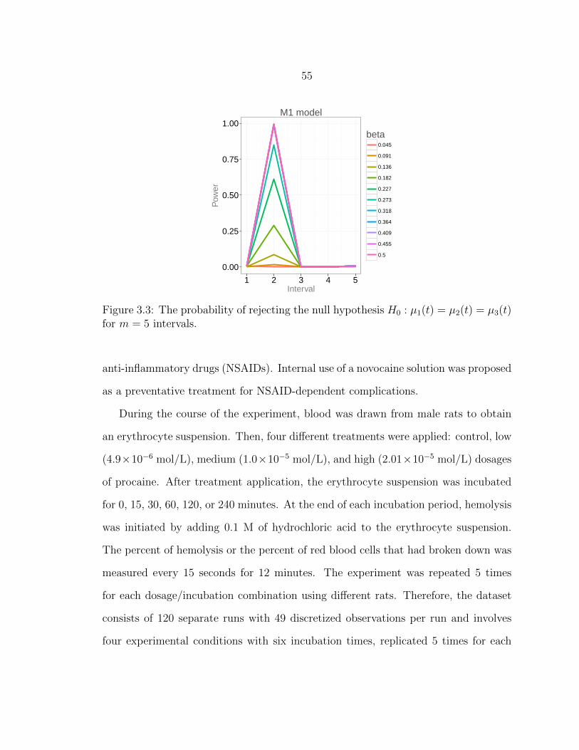
55

0.00

0.25

0.50

0.75

1.00

1 2 3 4 5Interval

Pow

er

beta0.045

0.091

0.136

0.182

0.227

0.273

0.318

0.364

0.409

0.455

0.5

M1 model

Figure 3.3: The probability of rejecting the null hypothesis H0 : µ1(t) = µ2(t) = µ3(t)for m = 5 intervals.

anti-inflammatory drugs (NSAIDs). Internal use of a novocaine solution was proposed

as a preventative treatment for NSAID-dependent complications.

During the course of the experiment, blood was drawn from male rats to obtain

an erythrocyte suspension. Then, four different treatments were applied: control, low

(4.9×10−6 mol/L), medium (1.0×10−5 mol/L), and high (2.01×10−5 mol/L) dosages

of procaine. After treatment application, the erythrocyte suspension was incubated

for 0, 15, 30, 60, 120, or 240 minutes. At the end of each incubation period, hemolysis

was initiated by adding 0.1 M of hydrochloric acid to the erythrocyte suspension.

The percent of hemolysis or the percent of red blood cells that had broken down was

measured every 15 seconds for 12 minutes. The experiment was repeated 5 times

for each dosage/incubation combination using different rats. Therefore, the dataset

consists of 120 separate runs with 49 discretized observations per run and involves

four experimental conditions with six incubation times, replicated 5 times for each

56

0.00

0.25

0.50

0.75

1.00

HAB : µ1=µ2 HAC : µ1=µ3 HBC : µ2=µ3

Hypotheses

Pro

babi

lity

of r

ejec

ting

the

null beta

0.136

0.182

0.227

0.273

0.318

0.364

0.409

0.455

0.5

M1 model

Figure 3.4: The probability of rejecting individual pairwise hypotheses HAB : µ1(t) =µ2(t), HAC : µ1(t) = µ3(t), and HBC : µ2(t) = µ3(t).

treatment/incubation combination. For more details see Holodov and Nikolaevski

(2012).

We fit the data with smoothing cubic B-splines with 49 equally spaced knots at

times t1 = 0, . . . , t49 = 720 seconds to generate the functional data. A smoothing

parameter was selected by generalized cross validation (GCV) for each functional

observation with an increased penalty for each effective degree of freedom in the

GCV, as recommended in Wood (2011).

To keep the analysis as simple as possible, each incubation data set was analyzed

for treatment effects separately. Our initial test was to check for a significant difference

in mean erythrograms (mean hemolysis curves) anywhere in time among novocaine

dosages. A Bonferroni correction was applied to these initial p-values to adjust for

multiplicity at this level. The results indicated strong evidence of differences for the

15 and 30 minute incubation times (p-valueBonf = 0.006 and p-valueBonf = 0.018

respectively). Figure 4.2 illustrates the results for these incubation times. For the

57

0.00

0.25

0.50

0.75

1.00

1 2 3 4 5Interval

Pow

er

beta0.045

0.091

0.136

0.182

0.227

0.273

0.318

0.364

0.409

0.455

0.5

M2 model

Figure 3.5: The probability of rejecting the null hypothesis H0 : µ1(t) = µ2(t) = µ3(t)in case of M2 model and 5 intervals.

rest of the incubation times, we found no evidence against the null hypothesis that

the four erythrogram means coincided so no further analysis was conducted.

Next, we examined the 15 and 30 minute incubation results in more detail to asses

the nature of the differences. For both incubation times, four time intervals of interest

were pre-specified: (i) the latent period (0-60 sec), (ii) hemolysis of the population

of the least stable red blood cells (61-165 sec), (iii) hemolysis of the general red

blood cell population (166-240 sec), and (iv) the plateau (over 240 sec). The latent

period is associated with erythrocytes spherulation and occurs between addition of the

hemolytic agent and initiation of hemolysis. The names of the next two periods are

self-explanatory. The plateau period is associated with deterioration of the population

of the most stable erythrocytes.

We applied our method to determine if statistical significance is present in each of

the four time intervals. In the application of our method, we set the p-values for the

global hypotheses H1234 of no significant difference on all four intervals to the Bonfer-

58

p−value=0.806

p−value=0.022

p−value=0.045

p−value=0.006

Low vs Control 0.022

Med vs Control 0.060

Low vs High 0.057


Med vs Control 0.016

High vs Control 0.030


0

20

40

60

80

0 200 400 600Time (sec)

Hem

olys

is %

Novocaine Dosage

control

low

medium

high

p−value=0.892

p−value=0.018

p−value=0.029

p−value=0.018

Low vs Control 0.018Medium vs Control 0.039Low vs High 0.030


Low vs Control 0.018Med vs Control 0.029High vs Control 0.029

0

20

40

60

80

0 200 400 600Time (sec)

Hem

olys

is %

Novocaine Dosage

control

low

medium

high

Figure 3.6: Erythrogram means for the control group and the treatment groups for15 (top graph) and 30 (bottom graph) minute incubation times

roni adjusted p-values obtained on the previous step. For the 15 minute incubation

time, no statistical significance was found during the latent period (p-value=0.806),

statistically significant results were found during hemolysis of the least stable red

blood cell population (p-value=0.022), general red blood cell population (marginal

significance with the p-value=0.060), and plateau (p-value=0.006). The same results

were obtained from the 30 minute incubation, i.e., no statistical significance during

59

the latent period (p-value=0.892) and statistical significance for the rest of the time

intervals with p-values of 0.018, 0.029, and 0.018 for the periods of hemolysis of the

least stable population, general population, and plateau respectively.

Finally, we were interested in pairwise comparison of treatment levels within the

time intervals of statistical significance. Once again, similar results were found for

both incubation times although the p-values were often larger for the 15 minute

incubation time. During the hemolysis of the least stable red blood cell population,

at least some evidence was found of a difference between low dosage and control

(p-value15=0.020, p-value30=0.018), medium dosage and control (p-value15=0.060, p-

value30=0.039), and low dosage and high dosage (p-value15=0.057, p-value30=0.030).

During the hemolysis of the general population, at least some evidence of a sig-

nificant difference was found between the low dose and control (p-value15=0.060, p-

value30=0.029). During the plateau interval, there was a significant difference between

low dose and control (p-value15=0.001, p-value30=0.018), medium dose and control

(p-value15=0.016, p-value30=0.029), and high dose and control (p-value15=0.030, p-

value30=0.029).

The results of the analysis can be summarized as follows. The rate of hemoly-

sis increases with the dosage of novocaine. That is, the structural and functional

modifications in the erythrocyte’s membrane induced by novocaine are dosage depen-

dent. The results also indicate the distribution of erythrocytes into sub-populations

with low, medium and high resistance to hemolysis. These populations modified by

novocaine react differently with the hemolytic agent. After 15 and 30 minutes of

incubation, the “old” erythrocytes (least stable) modified by low (4.9× 10−6 mol/L)

and medium (1.0× 10−5 mol/L) doses of procaine react faster to the hemolytic agent

than those under the control or the high (2.01×10−5 mol/L) dose. However, reaction

of the general and “young” (most stable) erythrocyte population modified by the

60

same (low and medium) dosages is characterized by higher stability of the membrane

and thus have higher resistance to the hemolytic agent. Thus, novocaine in low

and medium doses has a protective effect on the general and “young” erythrocyte

populations. However, an increase in procaine dosage does not lead to increase of

erythrocyte resistance to the hemolytic agent. The effect of the high dose of novo-

caine (2.01 × 10−5 mol/L) does not differ significantly from the control and thus is

destructive rather than protective.

Conclusions of our statistical analysis confirm certain findings reported in a patent

by Holodov and Nikolaevski (2012). Specifically, our analysis confirm that novocaine

in low dosages tends to have a protective effect. However, Holodov and Nikolaevski

(2012) reported a significant difference among erythrograms for all incubation times

but zero minutes. This inconsistency is due to a failure to properly control the tests

for the multiplicity in the original analysis. The findings reported in the current paper

provide a higher assurance that a replication experiment will be able to detect the

same differences reported here.

5. Discussion

We have suggested a procedure which allows researchers to find regions of signif-

icant difference in the domain of functional responses as well as to determine which

populations are different over these regions. To the best of our knowledge, there are

no existing competing procedures to the proposed methodology. Thus, our numerical

results reported in Section 3 do not include a comparison of the proposed method

to other alternatives. Nevertheless, the simulations revealed that our procedure has

satisfactory power and does a good job of picking out the differences between pop-

ulation means. Also, in our simulation study, a relatively small number of regions

61

(m = 5 and m = 10) was considered. A higher number of individual tests (intervals)

can be easily implemented with the described shortcut to the closure principle.

Note that the regions of interest in the functional domain should be pre-specified

prior to the analysis. However, in our experience researchers have never had a problem

with a priori region identification. From previous research, expected results as well

as specific regions of interest are typically known. We also mentioned that in the

application of our method the intervals should be mutually exclusive and exhaustive.

If researchers are interested in a test over overlapping intervals, the solution is to split

the functional domain into smaller mutually exclusive intervals for individual tests

(terminal nodes of the hypotheses tree). The decision for the overlapping region would

be provided by a test of an intersection hypothesis (“higher” node in the hypotheses

tree). We also expect the intervals to be exhaustive since it would be unexpected for

researchers to collect data over time periods that they have no interest in. Finally,

if for some reason distinct regions can not be prespecified, a large number of equal

sized intervals can easily be employed.

We could not find a method directly comparable to the proposed procedure, but

the present work has two open issues that suggest a direction for future research.

First, the method is conservative and so a more powerful approach may be possible.

Second, the permutation strategy for the pairwise comparison test may lead to biased

inference. Solutions to the latter problem were suggested both by Petrondas and

Gabriel (1983) and Troendle and Westfall (2011). We leave implementation of these

solutions for future research as this seems to be a minor issue with a small number

of treatment groups as are most often encountered in FANOVA applications.

62

β HAB : µ1 = µ2 HAC : µ1 = µ3 HBC : µ2 = µ3

0.318 0.027 0.021 0.0260.364 0.029 0.024 0.0280.409 0.031 0.034 0.0380.455 0.036 0.041 0.0470.500 0.036 0.049 0.054

Table 3.1: Power of the pairwise comparison assuming common means µ1 and µ2 overthe 1st interval, (M2) model


0.273 0.018 0.049 0.0570.318 0.025 0.074 0.0860.364 0.031 0.104 0.1160.409 0.037 0.145 0.1640.455 0.041 0.214 0.2240.500 0.045 0.298 0.323

Table 3.2: Power of the pairwise comparison assuming common means µ1 and µ2 overthe 2nd interval, (M2) model


0.182 0.015 0.038 0.0400.227 0.021 0.077 0.0840.273 0.027 0.160 0.1550.318 0.037 0.289 0.2750.364 0.041 0.437 0.4340.409 0.048 0.610 0.6000.455 0.048 0.731 0.7350.500 0.049 0.839 0.835

Table 3.3: Power of the pairwise comparison assuming common means µ1 and µ2 overthe 3rd interval, (M2) model

63


0.182 0.017 0.082 0.0800.227 0.023 0.207 0.1960.273 0.030 0.375 0.3650.318 0.036 0.618 0.6110.364 0.039 0.817 0.8070.409 0.041 0.920 0.9150.455 0.041 0.971 0.9710.500 0.041 0.993 0.993

Table 3.4: Power of the pairwise comparison assuming common means µ1 and µ2 overthe 4th interval, (M2) model


0.136 0.012 0.044 0.0420.182 0.020 0.164 0.1600.227 0.030 0.380 0.3830.273 0.038 0.640 0.6450.318 0.041 0.858 0.8590.364 0.042 0.955 0.9570.409 0.042 0.986 0.9880.455 0.042 0.997 1.0000.500 0.042 1.000 1.000

Table 3.5: Power of the pairwise comparison assuming common means µ1 and µ2 overthe 5th interval, (M2) model

64

References






Garcia-Rodriguez, L. A., Hernandez-Diaz, S., de Abajo, F. J., 2001. Associationbetween aspirin and upper gastrointestinal complications: Systematic review ofepidemiologic studies. British Journal of Clinical Pharmacology 52, 563–571.



Holodov, D. B., Nikolaevski, V. A., 2012. A method for preventing damages to thestomach mucous membrane when taking non-steroidal anti-inflammatory drugs.Patent RU 2449784.URL http://www.findpatent.ru/patent/244/2449784.html


Nasonov, E. L., Karateev, A. E., 2006. The use of non-steroidal anti-inflammatorydrugs: clinical recommendations. Russian Medical Journal 14 (25), 1769–1777.


Petrondas, D. A., Gabriel, K. R., 1983. Multiple comparisons by rerandomizationtests. Journal of the American Statistical Association 78 (384), 949–957.

http://www.findpatent.ru/patent/244/2449784.html

65






Troendle, J. F., Westfall, P. H., 2011. Permutational multiple testing adjustmentswith multivariate multiple group data. Journal of Statistical Planning and Inference141, 2021–2029.

Westfall, P. H., Young, S. S., 1993. Resampling-based Multiple Testing: Examplesand Methods for p-Values Adjustment. Wiley.

Wood, S. N., 2011. mgcv: generalized additive model method. R package version1.7-19.URL http://CRAN.R-project.org/package=mgcv



http://CRAN.R-project.org/package=mgcv

66

CHAPTER 4

RESAMPLING-BASED MULTIPLE COMPARISON PROCEDURE WITH

APPLICATION TO POINT-WISE TESTING WITH FUNCTIONAL DATA.



Contributions: Wrote the majority of the manuscript.



Co-Author: Dr. Scott. L. Powell

Contributions: Provided application expertise and feedback on drafts of the manuscript.

Co-Author: Dr. Dmitri V. Zaykin


67


Olga A. Vsevolozhskaya, Mark C. Greenwood, Scott L. Powell, Dmitri V. Zaykin

Environmental and Ecological Statistics


X Prepared for submission to a peer-reviewed journal

Officially submitted to a peer-review journal

Accepted by a peer-reviewed journal


Published Springer.

Submitted April, 2013

68

Abstract

In this paper we describe a coherent multiple testing procedure for correlated teststatistics such as are encountered in functional linear models. The procedure makesuse of two different p-value combination methods: the Fisher combination methodand the Sidak correction-based method. The distribution of Fisher’s and Sidak’s teststatistics are estimated through resampling to cope with the correlated tests. Buildingupon these two existing combination methods, we propose the smallest p-value as anew test statistic for each hypothesis. The closure principle is incorporated alongwith the new test statistic to obtain the overall p-value and appropriately adjust theindividual p-values. Furthermore, a shortcut version for the proposed procedure isdetailed, so that individual adjustments can be obtained even for a large numberof tests. The motivation for developing the procedure comes from a problem ofpoint-wise inference with smooth functional data where tests at neighboring pointsare related. A simulation study verifies that the methodology performs well in thissetting. We illustrate the proposed method with data from a study on the aerialdetection of the spectral effect of below ground carbon dioxide leakage on vegetationstress via spectral responses.

1. Introduction

High-dimensional data analysis is a current emphasis in statistical methodology

development. High-dimensional data consisting of observations measured “continu-

ously” in time are typically called functional data. Examples include longitudinal

data with subjects exposed continually to a certain treatment (Coull et al. (2000))

and more recently data obtained through Next Generation Sequencing (NGS) (Luo

et al. (2012)) with the position of a genetic variant in a genomic region playing the

role of time. Because in practice the continuous measurements are approximated by

a vector – a continuous function evaluated on a grid of L points ti, i = 1, . . . , L –

point-wise inference provides an intuitive and easy way to analyze functional data.

For example, Godwin et al. (2010) were interested in variability observed in human

motion patterns. By discretizing kinematic and kinetic lifting curves on a grid of

69

L = 100 points (and performing inference point-wise), they were able to demonstrate

additional areas of difference in motion patterns beyond those identified by tradi-

tional analysis based solely on peak values. However, conclusions based on a set

of L point-wise p-values may lead to far too many falsely significant tests (see Rice

(1988) for some numerical examples). In particular, although Godwin et al. (2010)

say that “additional areas outside of the peaks were significantly different,” they

concluded significance for all L = 100 points and all types of lifting curves. These

conclusions made the interpretation of findings troublesome. An adequate method for

simultaneous point-wise testing needs to account for potentially inflated false positive

results.

The commonly used Bonferroni correction for false positive decisions is not ideal

for point-wise inference with functional data. The Bonferroni procedure is designed

to correct for L independent simultaneous tests. If functional inference is performed

on a point-wise grid, the corresponding p-values at nearby time points are correlated

and the Bonferroni correction becomes overly conservative (Cribbie (2007)). Some

methods suggest replacing the number of tests L in the Bonferroni method by an es-

timate of the effective number of independent tests (Cheverud (2001), Nyholt (2004),

Li and Ji (2005)). The idea is to estimate the effective number of tests based on the

eigenvalue variance of the correlation matrix. However, the suggestion that a single

parameter, i.e., the number of independent tests, can fully capture the correlation

structure is rather simplistic.

Geologic carbon sequestration (GCS) is a carbon capture and storage technique

that could play a major role in climate mitigation strategy. Our work is motivated

by a problem of CO2 surface leakage detection from a GCS site. Since vegetation

is a predominant land cover over a GCS cite, Bellante et al. (2013) analyzed areal

hyperspectral images of the simulated CO2 leak site in attempt to identify differ-

70

ences in mean spectral signatures of healthy vegetation and vegetation under stress.

Specifically, Bellante et al. (2013) proposed the Red Edge Index (REI) – a single

test statistic that summarizes differences between the spectral signatures of healthy

and stressed vegetation. We used the data collected by Bellante et al. (2013) in an

attempt to identify specific wavelength regions where the mean spectral signatures

(mean spectral responses) of healthy vegetation and vegetation under stress differ (see

Figure 4.5). Our approach was to perform the analyses on a discretized grid of 80

points because the original spectral data were collected in 80 bands throughout the

visible and near infrared wavelengths (see Bellante et al. (2013) for a detailed data

collection description).

Although interest in point-wise inference is obvious, few viable approaches exist

in this direction that account for inflated false positive results and correlation struc-

ture among tests. Ramsay and Silverman (2005) proposed a method for performing

L point-wise tests simultaneously, however fail to adjust the results to control the

family-wise error rate (FWER), the probability of at least one false rejection of all

the tests. A more promising approach was introduced by Cox and Lee (2008) who

used the multiplicity correction procedure proposed by Westfall and Young (1993) to

control the FWER. Additionally, neither of the proposed methods provide a decision

regarding the overall null hypothesis that all single L hypotheses are true. This is

an undesirable property since a multiple comparison procedure may be non-coherent

(Gabriel (1969)), i.e., the rejection of at least one individual hypothesis may not imply

the rejection of the global null, which might lead to interpretation problems.

In this paper, we propose a point-wise procedure that both provides a decision

for the overall hypothesis and adequately adjusts the individual p-values to account

for L simultaneous tests. The method first uses two different p-value combining

methods to summarize the associated evidence across L points, defines a new test

71

statistic, W , based on the smallest p-value from the two combination methods, and

applies the closure principle of Marcus et al. (1976) to individually adjust the L

point-wise p-values. The idea of using the minimum p-value as the test statistic

for the overall test across different combination methods has been used in multiple

genetics studies (Hoh et al. (2001), Chen et al. (2006), Yu et al. (2009)). A challenge

for the proposed analysis was the individual adjustment performed using the closure

principle. The closure principle generally requires 2L − 1 tests. To overcome this

obstacle, we describe a computational shortcut which allows individual adjustments

using the closure method even for large L. Accordingly, the paper is organized as

follows. We give an overview of the closure principle and detail the computational

shortcut to it. We give an explicit strategy for the proposed approach and compare

its performance to other possibilities in a simulation study. We apply the proposed

methodology in order to identify regions of the electromagnetic spectrum that differ

based on distances to a simulated underground CO2 leak.

2. Multiple Tests and Closure Principle

2.1. The General Testing Principle

It is well known that by construction all inferential methods have a nonzero proba-

bility of Type I error. Therefore, when L multiple tests are conducted simultaneously,

the probability of finding at least one spurious result is greater than the threshold

α. A multiple test adjustment procedure, which controls a family-wise error rate for

the family of individual hypotheses, H1, . . . , HL, at a pre-specified level α, can be

obtained through the closure principle of Marcus et al. (1976). The closure principle

considers all possible combination hypotheses obtained via the intersection of the set

of L individual hypotheses HI = ∩{Hi : i ∈ I}, I ⊆ {1, . . . , L}. The coherence

72

of the procedure is enforced by rejecting an individual hypothesis Hi, i = 1, . . . , L,

only if all intersection hypotheses that contain it as a component are rejected. Most

researchers prefer the results of a multiple test procedure to be presented in terms of

L individually adjusted p-values. The individually adjusted p-value for the hypothesis

Hi is set to the maximum p-value of all intersection hypotheses implied by Hi.

A valuable feature of the closure principle is its generality, i.e., any suitable α-level

test can be used to test the intersection hypotheses. However, the implementation of

the method becomes computationally challenging for a large number of tests. The

total number of intersection hypotheses is 2L − 1 which grows quickly with L and

limits the applicability of the method. Grechanovsky and Hochberg (1999) exhaus-

tively discussed the conditions under which the closure procedure admits a shortcut.

However, the discussion in Grechanovsky and Hochberg (1999) is motivated by the

case of joint multivariate normal test statistics and the question remains of how to

reduce the computational burden of the closure method in the case of non-normal

correlated tests.

2.2. Closure in a Permutation Context

Permutation-based methods are becoming more popular for multiple testing cor-

rections with high-dimensional data. They do not require normality assumptions and

utilize the data-based correlation structure. That is, the resulting procedure for false

positive decision corrections based on permutation test is exact despite unknown co-

variance structure (unlike the Bonferroni procedure that tends to be over conservative

for correlated tests). The closure method easily admits permutation-based tests, all

that is required is an α-level permutation test for each intersection hypothesis. West-

fall and Troendle (2008) described a computational shortcut for the closure principle

with a permutation test that reduces the number of required computations from the

73

order of 2L to L. The drastic reduction in computational burden is achieved by (i)

testing each intersection hypothesis HI with either a min-p test statistic (mini∈I pi,

where pi is the individual p-value) or a max-t statistic (maxi∈I tI , where ti is the

individual test statistic), and (ii) the assumption of subset pivotality. However, there

are other more powerful test statistics one can use to test an intersection hypothesis

HI . Here, we show how to implement a computational shortcut for the Sidak (Sidak

(1967)) and Fisher (Fisher (1932)) permutation-based tests to reduce the number of

computations from the order of 2L to the order of L2.

Suppose K tests are conducted and the resulting p-values are p1, . . . , pK . Denote

the ordered p-values by p(1) ≤ · · · ≤ p(K). The test based on the Sidak correction for

the intersection of K hypothesis, ∩Ki=1Hi, is

SK = 1− (1− p(1))K . (4.1)

The Fisher test statistic for the same intersection hypothesis is

FK = −2K∑i=1

ln pi. (4.2)

The permutation p-values based on the Sidak correction are equivalent to the p-values

based on the min-p test statistic and the rank truncated product statistic (RTP),

W (K) =∏K

i=1 p(i), of Dudbridge and Koeleman (2003) with truncation at K = 1.

The equivalence is due to the fact that 1− (1− p(1))K is a monotonic transformation

of p(1). Similarly, −2∑K

i=1 ln pi is a monotonic transformation of∏K

i=1 p(i), and the

permutation p-values based on these two test statistics are equivalent.

The idea behind the shortcut is to consider only the “worst” (the smallest)

test statistic in the subsets of the same cardinality. Note that, for both the Sidak

74

correction-based test and the Fisher test, the values of the test statistics are mono-

tonically decreasing among intersection hypotheses of the same size. Thus, for the

ordered p-values, p(1) ≤ · · · ≤ p(L), the hypotheses that will be used for individual

adjustments are:

for H1, {H1,H1L,H1L(L−1), . . . ,H1L...2};

for H2, {H2,H2L,H2L(L−1), . . . , H2L...1};

for H3, {H3,H3L,H3L(L−1), . . . , H3L...1};...

...

for HL, {HL, HL(L−1), HL(L−1)(L−2), . . . , HL(L−1)...1}.

Here, the hypothesis H1 has p-value p(1), H2 has p-value p(2), etc. The unique intersec-

tion hypotheses to consider are highlighted in bold, and the number of unique tests to

consider is 1 + 2 + · · ·L = L(L+1)2

. One need not necessarily use resampling to apply

the above shortcut, however it also works well if permutations are used to find p-

values for each intersection hypothesis. Figure 4.1 illustrates correspondence between

p-values calculated based on the full closure “resampling-based” procedure and the

“resampling-based” shortcut. The graphs show an excellent agreement between the

two adjusted p-values for both Sidak and Fisher test statistics. To obtain the plots,

L = 10 p-values were simulated B = 20 times from the Unif (0,1) distribution and

corrected using the full closure and the computational shortcut. Considering the

adjustments for more than L = 10 p-values was impractical due to the computational

burden of the full closure procedure.

75

0.00

0.25

0.50

0.75

1.00

0.00 0.25 0.50 0.75 1.00

Shortcut Individually Adjusted Sidak p−values

Ful

l Clo

sure

Indi

vidu

ally

Adj

uste

d S

idak

p−

valu

es

0.4

0.6

0.8

1.0

0.4 0.6 0.8 1.0

Shortcut Individually Adjusted Fisher p−values

Ful

l Clo

sure

Indi

vidu

ally

Adj

uste

d F

ishe

r p−

valu

es

Figure 4.1: Correspondence between individually adjusted p-values using the fullclosure algorithm and the computational shortcut (L = 10). The Sidak p-values areillustrated in the left panel, and the Fisher p-values in the right panel.

3. Proposed Methodology

We now describe a permutation algorithm that ensures coherency when estimating

adjusted individual p-values. Suppose L correlated tests are conducted simultane-

ously. Apply the following steps to obtain the corresponding individually adjusted

p-values.

1. Construct L(L+1)2×(B+1) matrices of Sidak and Fisher permuted test statistics,

Sij, Fij, i = 1, . . . , L(L+1)2

(indexes intersection hypotheses), j = 1, . . . , B + 1

(indexes permutations). The first column of the matrices contains the observed

test statistics.

2. Construct L(L+1)2× (B + 1) matrices of the permuted p-values based on the

algorithm from Ge et al. (2003) – discussed below. The Sidak p-value for the

i-th intersection hypothesis and j-th permutation is

P sij =

1

B

B+1∑k=1,k 6=j

I(Sik ≤ Sij).

76

The Fisher p-value for the i-th intersection hypothesis and j-th permutation is

P fij =

1

B

B+1∑k=1,k 6=j

I(Fik ≥ Fij).

3. Define the statistic Wij = min(P Sij , P

fij) and obtain its p-value as

PWi =

1

B

B+1∑k=2

I(Wik ≤ Wi1), i = 1, . . . ,L(L+ 1)

2.

4. Make an overall decision and obtain L individually adjusted p-values by applying

the closure principle to the set of PWi ’s.

To avoid nested permutations in Step 2, we used the algorithm by Ge et al. (2003)

to compute permutational p-values for each permutation j = 2, . . . , B + 1. More

specifically, the algorithm allows one to obtain permutational p-values in the closure

based on just B permutations instead of B2. Also, in Step 3, testing the ith intersec-

tion hypothesis with Wij at a threshold α would lead to inflated Type I error rate,

because choosing the smallest of the two p-values P Sij and P f

ij leads to yet another

multiple testing problem. To overcome this issue, one can use either the Bonferroni

correction and define the test statistic as 2 min(P s, P f ) or, as suggested, determine

the significance of W on the basis of permutations. Finally, setting W = min(P S, P f )

is the same as min(RTP(1),RTP(L)), where RTP(·) is the rank truncated product

statistic of Dudbridge and Koeleman (2003) but also considered in Zaykin (2000) and

Zaykin et al. (2007). Thus, W incorporates two extremes: the combination of all

p-values and a min-p adjustment procedure. Simulation studies are used to show it

retains desired properties of both type of statistics.

77

4. Simulations

4.1. Simulation Study Setup

We were motivated by a problem of identifying differences in mean spectral signa-

tures of healthy vegetation and vegetation under stress across electromagnetic spectra.

We approach the problem by evaluating functional responses on a grid of 80 points

across wavelengths and performing tests point-wise. More generally, we were inter-

ested in evaluating k groups of functional responses on a grid of L points, t1, . . . , tL,

and performing point-wise inference in the functional data setting. The goal of the

simulation study was to investigate the power of the proposed procedure to detect

departures from (1) the global null hypothesis ∩Li=1Hi of no difference anywhere in t

and (2) the point-wise null hypotheses H0 : µ1(ti) = µ2(ti) for all ti, i = 1, . . . , L. We

followed the setup of Cox and Lee (2008) and for all simulations generated two samples

of functional data with n1 = n2 = 250 observations in each group (N = 500). The

mean function of the first sample was constant and set to zero, µ1(t) ≡ 0, t ∈ [0, 1].

The mean of the second sample was either set to µ2(t) = γBeta(1000, 1000)(t) or

µ3(t) = γBeta(5, 5)(t), where Beta represents probability density function of the

Beta distribution. Figure 4.2 illustrates µ2(t) and µ3(t) for the range of different γ

values explored.

First, we simulated the case where all L point-wise hypotheses were true (µ1(ti) ≡

µ2(ti) ∀ti). To obtain functional data, we evaluated the mean functions on a grid

of 140 equally spaced points ranging from -0.2 to 1.2 and added random noise,

εij ∼ N(0, 0.012). Then, we fitted a smoothing spline using the smooth.spline R

function (R Core Team (2013)) with the 0.95 smoothing parameter for each functional

observation as suggested in Cox and Lee (2008). The output of the smooth.spline

function is the fitted values of functional responses evaluated on the original grid of

78

µ2(t)

µ3(t)0.0000

0.0025

0.0050

0.0075

0.00 0.25 0.50 0.75 1.00Time

Mea

n0.000100.000150.000200.00025

γ

Figure 4.2: Two choices for the mean of the second sample.

points. We disposed of 20 points from each end to remove excessive boundary vari-

ability from the estimated splines and for each curve sub-sampled 50 equally spaced

values on the grid between 0 and 1. At the 0.05 level, we evaluated the empirical Type

I error rate for the global null and the control of the FWER in a weak sense (meaning

that all observations come from the null hypothesis) for the proposed procedure and

five alternative statistical methods: the Sidak correction based test, the Fisher test,

the Cox and Lee method (Cox and Lee (2008)), the functional F statistic (Shen and

Faraway (2004)), and the functional Vn (Cuevas et al. (2004)).

The functional test statistics of Shen and Faraway (2004) and Cuevas et al. (2004)

are designed to perform the overall functional analysis of variance (FANOVA) test.

The FANOVA null and alternative hypotheses are

H0 : µ1(t) = µ2(t) = . . . = µk(t)

Ha : µi(t) 6= µi′(t), for at least one t and i 6= i′,

79

where µi(t) is assumed to be fixed, but unknown, population mean function of group

i, i = 1, . . . , k. Parametric distributions are available for both F and Vn from the

original papers. The FANOVA test assesses evidence for the existence of differences

among population mean curves in the entire functional domain. The test across the

entire t is a global test. Thus, we considered these two methods as competitive to

the proposed methodology.

Second, we investigated two properties of our method: (1) power to detect devi-

ations from the combined null hypothesis ∩Li=1Hi and (2) power to detect deviations

from point-wise hypotheses H1, H2, . . . , HL. To calculate power for the combined null

hypotheses, we simulated B = 1000 sets of functional observations for the specified

range of γ values, performed the overall test and calculated the empirical probability

of rejecting ∩Li=1Hi. At the point-wise level, the concept of power is not as clear cut.

For example, one may calculate conjunctive power – the probability of rejecting all

false null hypotheses – or disjunctive – the probability of rejecting at least one false

hypothesis. For a detailed discussion of these different choices see Bretz et al. (2010).

Here, we adopted the approach of Cox and Lee (2008) to be able to directly compare

to their results. We considered a single simulated set of functional observations for

a specific choice of γ; calculated the unadjusted point-wise p-values; performed the

multiplicity adjustment using W , as well as by Fisher’s, Sidak’s, and Westfall-Young

method; then we compared the adjusted p-values by plotting them on a single graph.

4.2. Results

Table 4.1 summarizes control of the Type I error rate for the overall null hy-

pothesis, ∩Li=1Hi, and the family-wise error rate (FWER) in the weak sense for the

point-wise tests (i.e., ∩Li=1Hi is true). All methods tend to be liberal in terms of the

Type I error rate control (“combined null” line). The family-wise error rate is inflated

80

for Sidak’s test, too conservative for Fisher’s test, and right on the 0.05 margin for

the Westfall-Young adjustment.

Sidak Fisher W Cox and Lee F Vncombined null 0.059 0.065 0.060 NA 0.059 0.057FWER 0.059 0.000 0.036 0.049 NA NA

Table 4.1: The Type I error for the global null (∩Li=1Hi) and the FWER for L = 50tests, 1000 simulations, and α = 0.05.

Figure 4.3 illustrates power for the global null hypothesis (∩Li=1Hi). We see that

in both graphs Fisher’s method outperforms all of the other methods, however W

has similar power for this realization. The performance of the functional F of Shen

and Faraway (2004) is very similar to the functional Vn of Cuevas et al. (2004). The

Sidak test is the clear laggard.

µ2(t)

0.00

0.25

0.50

0.75

1.00

0.00005 0.00030γ

Pow

er

WFisherSidakShenCuevas

µ3(t)

0.00

0.25

0.50

0.75

1.00

0.00005 0.00030γ

Pow

er

WFisherSidakShenCuevas

Figure 4.3: Plots of empirical power for the combined null hypothesis with α = 0.05.

81

Figure 4.4 shows the unadjusted and the adjusted p-values for a single set of

functional observations. To compute the unadjusted p-values, we simulated 250 curves

with mean µ1(t) = 0 and µ2(t) = 0.0003Beta(1000, 1000)(t) (left graph) or µ1(t) = 0

and µ3 = 0.0003Beta(5, 5)(t) (right graph) and performed a t-test on a grid of 50

equally spaced points t1 = 0, . . . , t50 = 1. From both graphs, it is evident that

Fisher’s method has the lowest power. The performance of W is very similar to

Sidak’s test. The Westfall–Young method has the highest power.

0.00

0.25

0.50

0.75

1.00

0 25 50 75 100

Time

P−

valu

es FisherSidakWWestfall−YoungUnadjusted

0.00

0.25

0.50

0.75

1.00

0 25 50 75 100

Time

P−

valu

es FisherSidakWWestfall−YoungUnadjusted

Figure 4.4: Plots of point-wise adjusted p-values for γ = 0.0003. Left graph: Hi :µ1(ti) = µ2(ti), i = 1, . . . , L. Right graph: Hi : µ1(ti) = µ3(ti), i = 1, . . . , L.

5. Application to Carbon Dioxide Data

Bellante et al. (2013) conducted an experiment to study the effect of carbon diox-

ide (CO2) surface leak on vegetation stress at the Montana State University Zero

Emission Research and Technology (ZERT) site in Bozeman, MT. To study the spec-

82

tral changes in overlying vegetation in response to elevated soil CO2 levels, a time

series of aerial images were acquired over a buried carbon dioxide release pipe. A

single image acquired on June 21, 2010 was the focus of the current analysis. The

pixel-level measurements (with nearly 32,000 pixels) of the image consist of 80 spec-

tral responses ranging from 424 to 929 nm. For each pixel, a horizontal distance

to the CO2 release pipe was calculated and 500 spectral responses were randomly

chosen from five distance subcategories: (0,1], (1,2], (2,3], (3,4], and (4,5] meters (see

Figure 4.5). To obtain a functional response for each pixel, we used the penalized

cubic B-spline smoother with a smoothing parameter determined by generalized cross-

validation (Ramsay et al. (2012)). The functional responses were evaluated on the

original grid of L = 80 points and subsequently the analysis of variance test was

performed point-wise to obtain the unadjusted p-values.

Visible

Red Edge

Near Infrared

0

5000

10000

15000

400 600 800Wavelength

Pix

el R

adia

nce

dist(0,1](1,2](2,3](3,4](4,5]

Figure 4.5: Spectral responses from 2,500 pixels corresponding to five different binneddistances with superimposed fitted mean curves.

83

First, we tested the global null hypothesis of no difference in the entire range of

spectral responses based on the distance from the CO2 release pipe and obtained

the corresponding overall p-value of 0.001 (from 1000 permutations) using W . We

then obtained the corrected point-wise p-values, which are illustrated in Figure 4.6.

The adjusted p-values from 700 to 750 nm were below α = 0.05 and correspond to

the “red edge” spectral region, which indicates that the spectral responses among

binned distances differ significantly within this region. This is an encouraging result

since previous research has indicated that the “red edge” spectral region is typically

associated with plant stress (Carter and Knapp (2001)).

The method proposed by Cox and Lee (2008), which employs the Westfall-Young

correction for multiplicity, identifies a much larger region of wavelengths than the

other methods. On the one hand, these additional discoveries may contribute to the

higher power of the method. On the other hand, these result may be due to inflated

FWER control in the strong sense. That is, we suspect that in the application

the p-values come from a mixture of the null and the alternative hypotheses. Our

simulations provided the FWER control only for a situation when all observations

came from the null hypothesis. More research is required in this direction to make

more conclusive statements.

6. Discussion

Modern data recording techniques allow one to sample responses at a high time

resolution. In many applications it is of interest to utilize all of the recorded infor-

mation and perform a test at each point, while accounting for the correlation of the

test statistics at nearby times, properly controlling the probability of false positive

findings, and providing information on the overall difference. Here, we suggested a

84

0.00

0.25

0.50

0.75

1.00

400 500 600 700 800 900Wavelength (nm)

p−va

lues

FisherSidakWWestfall−YoungUnadjusted

Figure 4.6: Plots of unadjusted and adjusted p-values. A horizontal line at 0.05 isadded for a reference.

coherent method for point-wise testing with the desired properties. Our approach was

inspired by methods used in genetic association studies, but extends these ideas and

allows for obtaining individually adjusted p-values in the case of multiple correlated

tests.

Our method capitalizes on the evidence based on the minimum p-value (the Sidak

method) and the product (or the sum on the logarithmic scale) of all p-values (the

Fisher method). This results in a procedure that has high power for the combined null

hypothesis, ∩Li=1Hi, and for the individual tests H1, H2, . . . , HL. These characteristics

of our procedure can be better understood by examining rejection regions of Fisher’s

and Sidak’s tests. In general, rejection regions for L tests are hypervolumes in L-

dimensional space, however some conclusions can be drawn from considering just

two p-values. The two-dimensional rejection regions for Fisher’s and Sidak’s tests

are provided in Loughin (2004). Based on the rejection regions, a clear difference is

evident between the Fisher method and the Sidak method. In particular, the Fisher

85

method will reject the combined null hypothesis, ∩Li=1Hi, if at least some p-values

are “small enough”, but not necessarily significant. The Sidak method will reject

the combined null hypothesis only if min-p is significant. Thus, Fisher’s method is

higher-powered than Sidak’s method for the overall null hypothesis. On the other

hand, Fisher’s test along with the closure principle is lower-powered than Sidak’s

method for the individual adjustments. Envision a situation where the smallest p-

value, p(1), is just above α. The adjusted value of p(1) by the closure principle is

the maximum p-value of all hypotheses implied by H(1). To test an intersection

hypothesis of size K, Fisher’s test considers the combination of p(1), p(L), . . . , p(L−K+1).

All p(L), . . . , p(L−K+1) are greater than p(1) and Fisher’s test will not be able to reject

∩Ki=1Hi and thus H(1). Conversely, the decision for ∩Ki=1Hi based on Sidak’s test is

made regardless of the magnitudes of p(L), . . . , p(L−K+1) but solely on the magnitude of

p(1). Thus, the Sidak method along with closure principle has higher power than the

Fisher method for the individual tests H1, H2, . . . , HL. Since our approach combines

the Fisher and the Sidak method, it possesses desirable properties of both tests and

has high power for all ∩Li=1Hi and H1, H2, . . . , HL.

Our method is permutation-based. Generally, a drawback of the permutations

methods is their computational intensity. However, there is a big advantage to using

permutation-based methods. Cohen and Sackrowitz (2012) note that stepwise mul-

tiple testing procedures (including the closure principle) are not designed to account

for a correlation structure among hypotheses being tested. That is, test statistics

for an intersection hypothesis will always be the same regardless of the correlation

structure among tests considered. Thus, the shortcoming of the stepwise procedures

is determining a correct critical value. The permutation-based approach alleviates

this shortcoming and allows for dependency to be incorporated into the calculation

of the critical values.

86

Another advantageous property of our method is that it does not require access to

the original data but only to the L unadjusted point-wise p-values. The matrices of the

test statistics in Step 1 can be found based on the Monte Carlo algorithm described in

Zaykin et al. (2002). The test statistics are found by first obtaining L×1 vectors, R∗,

of independent random values from the Unif (0,1) distribution and then transforming

them to R – vectors with components that have the same correlation structure as

the observed p-values. Since functional observations are evaluated on a dense grid

of points, the correlation structure among observed p-values can be estimated with

reasonable precision. Thus, our method efficiently employs information contained just

in the p-values and is more flexible than methods that require access to the original

observations.

In summary, we proposed a coherent p-value combination method that allows

researchers to obtain individually adjusted p-values for multiple simultaneous corre-

lated tests. We hope that our work will promote new research in this direction. In

particular, in our approach we treated all p-values as equally important. It might

be possible to incorporate some weights that would optimize desirable properties of

the procedure based on a particular application. Alternatively, adaptive selection of

the test statistic is possible. That is, instead of considering just min-p (RTP(1)) and

the combination of all p-values (RTP(L)), one might optimize power and size of the

proposed method by considering RTP(K) across all possible values of K = 1, . . . , L.

Software

A sample script to adjust the point-wise p-values with the proposed method

is available at http://www.math.montana.edu/~vsevoloz/fanova/minSF/. The

http://www.math.montana.edu/~vsevoloz/fanova/minSF/

87

script requires users to provide a vector of unadjusted point-wise p-values. The

authors welcome questions regarding script usage.

88

References


Bretz, F., Hothorn, T., Westfall, P., 2010. Multiple Comparisons Using R. Chapman& Hall/CRC.

Carter, G., Knapp, A., 2001. Leaf optical properties in higher plants: linking spectralcharacteristics to stress and chlorophyll concentration. American Journal of Botany88, 677–684.


Cheverud, J., 2001. A simple correction for multiple comparisons in interval mappinggenome scans. Heredity 87, 52–58.


Coull, B., Catalano, P., Godleski, J., 2000. Semiparametric analysis of cross-over datawith repeated measures. Journal of Agricultural, Biological, and EnvironmentalStatistics 5 (4), 417–429.




Dudbridge, F., Koeleman, B., 2003. Rank truncated product of p-values, with appli-cation to genomewide association scans. Genetic Epidemiology 25, 360–366.

Fisher, R., 1932. Statistical Methods for Research Workers. Oliver and Boyd, London.

Gabriel, K. R., 1969. Simultaneous test procedures – some theory of multiple com-parison. Annals of Mathematical Statistics 40, 224–250.

89

Ge, Y., Dudoit, S., Speed, T., 2003. Resampling-based multiple testing for microarraydata analysis. Test 12, 1–44.

Godwin, A., Takaharab, G., Agnewc, M., Stevensond, J., 2010. Functional data anal-ysis as a means of evaluating kinematic and kinetic waveforms. Theoretical Issuesin Ergonomics Science 11 (6), 489–503.

Grechanovsky, E., Hochberg, Y., 1999. Closed procedures are better and often admita shortcut. Journal of Statistical Planning and Inference 76, 79–91.


Li, J., Ji, L., 2005. Adjusting multiple testing in multilocus analysis using the eigen-values of a correlation matrix. Heredity 95, 221–227.

Loughin, T., 2004. A systematic comparison of methods for combining p-values fromindependent tests. Computational Statistics & Data Analysis 47, 467–485.



Nyholt, D., 2004. A simple correction for multiple testing for single-nucleotide poly-morphisms in linkage disequilibrium with each other. American Journal of HumanGenetics 74, 765–769.




Rice, W., 1988. Analyzing tables of statistical tests. Evolution 43 (1), 223–225.


Sidak, Z., 1967. Rectangular confidence regions for the means of multivariate normaldistributions. Journal of the American Statistical Association 78, 626–633.



90

Westfall, P., Troendle, J., 2008. Multiple testing with minimal assumptions. Biomet-rical Journal 50, 745–755.

Westfall, P. H., Young, S. S., 1993. Resampling-based Multiple Testing: Examplesand Methods for p-Values Adjustment. Wiley.


Zaykin, D. V., 2000. Statistical analysis of genetic associations. Ph.D. thesis. NorthCarolina State University.

Zaykin, D. V., Zhivotovsky, L. A., Czika, W., Shao, S., Wolfinger, R. D., 2007.Combining p-values in large-scale genomics experiments. Pharmaceutical Statistics6 (3), 217–226.


91

CHAPTER 5

GENERAL DISCUSSION.

In this work, we presented procedures that allow for the extension of the overall

functional analysis of variance hypothesis testing. Our procedures capitalize on the

closure method along with the different combination methods of the test statistics

or the p-values. The closure multiplicity testing proved to be highly flexible since

different α-level tests can be employed to test different intersection hypotheses. Next,

we discuss limitations of the proposed methodology and outline direction for future

research.

In Chapter 2, we introduced the idea of a combining function as a weighted sum

of the observed test statistics. We also mentioned an extreme case of weights (all but

one are zeros) used by Ramsay et al. (2009). In our procedure we employ an equal-

weight combining function, however we think that incorporation of different weights

is really promising for improving the procedure in terms of size and power. Also, in

Chapter 2 we gave little weight to the discussion of the computational intensity of

the simulation studies with functional data. Despite escalating computing power, it

is still hard to handle extensive simulations and investigate all the desired properties

of a procedure. We briefly mentioned the Boos and Zhang (2000) method of power

extrapolation based on a set of 59/39/19 permutations. We also talked about a need

for an efficient computational shortcut to the closure procedure. Based on referee

feedback, we removed a discussion of the permutation strategy with the functional

responses. To speed up permutations, we employed a distance-based permutational

multivariate analysis of variance (perMANOVA) method of Anderson (2001) imple-

mented in the vegan R package(Oksanen et al. (2012)). The package allows one to

92

compute a pseudo-F statistic (Anderson (2001)) – equivalent to the functional F

(Shen and Faraway (2004)) – and provides an efficient distance-based permutation

strategy. For future research, it might be of interest to investigate further connections

between FANOVA and perMANOVA and make some generalizations.

In Chapter 3, we discussed a method that controls for multiple testing of all pair-

wise differences. It would be of interest to see if the proposed methodology satisfies the

“interval property”. If a procedure lacks the interval property, it could reject the null

hypothesis in one instance, and fail to reject it in a situation when intuitively we have

“stronger” evidence against the null hypothesis. The lack of the interval property

in a one-way ANOVA for testing all pair-wise differences is shown in Cohen et al.

(2010). In Cohen and Sackrowitz (2012), a residual based multiple testing procedure

for pairwise differences is introduced that does have the interval property. It would

be of interest to explore the interval property in the FANOVA setting and develop a

procedure that satisfies it. Another possibility of further extension of the proposed

methodology involves testing of treatment versus control problems and change point

problems.

In Chapter 4, we introduced a procedure that allows one to adjust L correlated

p-values for multiplicity as well as to combine information across K multiple tests,

i.e., test an intersection hypothesis ∩Ki=1Hi. The motivation for the study came from a

problem of point-wise testing in the FANOVA setting. For the two-group comparison

the point-wise null hypothesis is H0 : µ1(t) = µ2(t) for each t versus a two-sided

alternative Ha : µ1 6= µ2. However, in certain situations combining two-sided p-values

is undesirable because they disregard the effect direction. For example, imagine a

replication study in which the effect direction is flipped but both two-sided p-values

are small. The resulting combined p-value is going to be small and will promote

false conclusions. However, the combined result of the corresponding one-sided p-

93

values will properly reflect the change in the effect size direction. A simple way of

taking the effect size into consideration is presented in Zaykin (2011). This method

allows one to convert a two-sided p-value into a one-sided p-value and vice versa. It

also allows incorporation of different weights like the square root of the sample size.

Integration of this method into the procedure presented in Chapter 4 might broaden

its applicability.

Chapter 4 also discussed the issue of individual adjustment of many correlated

tests. Our solution to the test dependency problem was to use a permutation-based

method to find the p-values for each intersection hypothesis. The solution to the

plethora of tests was presented in a form of a shortcut to the closure principle of

Marcus et al. (1976). However, the temporal correlation might be directly incorpo-

rated into the calculation of a test statistic. The idea is to combine p-values that are

separated up to the points in time at which the correlation extinguishes. If L non-

independent tests are performed and pi, i = 1, . . . , L, are the corresponding p-values,

the test statistic will be

W =L∏i=1

pwii ,

where wi are some weights based on the distance between points. For example, assume

that we have a temporal correlation up to lag 2 and we are interested in testing five

individual hypotheses over time points t1, . . . , t5. We would incorporate distance

between time points into the construction of the intersection test statistics (Figure

5.1) and assign zero weights to the p-values that are “far apart” (Figure 5.2). The

idea is inspired by the work in Zaykin (2000), Zaykin et al. (2002), and Dudbridge

and Koeleman (2003). In Zaykin (2000) and Zaykin et al. (2002) the weights were

94

assigned based on a truncation point τ , i.e., wi = I(pi ≤ τ). In Zaykin (2000) and

Dudbridge and Koeleman (2003) the p-values up to rank k were combined.

H12345

H1234 H1235 H1245 H1345 H2345

H123 H124 H134 H234 H235 H145 H245 H345H125 H135

H12 H13 H23 H14 H24 H34 H15 H25 H35 H45

H1 H2 H3 H4 H5

Figure 5.1: The closure set formed by five individual hypotheses. The intersectionhypotheses that correspond to time points “far apart” are highlighted in blue.

Finally, applicability of the FANOVA can be extended to data sets that tradi-

tionally are not considered “functional.” Specifically, Luo et al. (2012) studied the

association between a quantitative trait and genetic variants in a genomic region.

Quantitative trait was treated as a scalar response. Genotype profile was considered

to be a function of a genomic position. Luo et al. (2012) tested for the additive effect

of a marker at the genomic position t across the entire genomic region. That is, if t

95

H12345

H1234 H1235 H1245 H1345 H2345

p1p2p3 p1p2p4 p1p3p4 p2p3p4 p2p3p5 1p4p5 p2p4p5 p3p4p5p1p21 p1p3p5

p1p2 p1p3 p2p3 1× 1 p2p4 p3p4 1× 1 1× 1 p3p5 p4p5

H1 H2 H3 H4 H5

Figure 5.2: The p-values corresponding to time points “far apart” are assigned zeroweights.

is a genomic position, a genomic profile Xi(t) of the i-th individual is:

Xi(t) =

1, MM

0, Mm

−1, mm

.

Yi is a quantitative phenotype value of the i-th individual and a functional linear

model for a quantitative trait can be written as:

Yi = µ+

∫ T

0

Xi(t)α(t)dt+ εi,

96

where εi ∼ N(0, σ2), T is the length of the genome region, and α(t) is a function

of the genetic additive effect of the marker at the genomic position t. What can

we do differently? We can “flip” the relationship, i.e., try to determine if there is a

significant difference among SNP’s with minor and major allele frequency based on

a certain categorical phenotype (like the presence or absence of a disease). We are

planning to investigate the performance of the FANOVA methodology in this setting

in future research.

97

References

Anderson, M. J., 2001. A new method for non-parametric multivariate analysis ofvariance. Austral Ecology 26, 32–46.



Cohen, A., Sackrowitz, H. B., Chen, C., 2010. Multiple testing of pairwise com-parisons. Borrowing Strength: Theory Powering Applications – A Festschrift forLawwrence D. Brown. IMS Collections 6 (144-157).






Shen, Q., Faraway, J., 2004. An f test for linear models with functional responses.Statistica Sinica 14, 1239–1257.


Zaykin, D. V., 2011. Optimally weighted z-test is a powerful method for combiningprobabilities in meta-analysis. Journal of Evolutionary Biology 24 (8), 1836–1841.



98

REFERENCES CITED

99

Abramovich, F., Antoniadis, A., Sapatinas, T., Vidakovic, B., 2002. Optimal testingin functional analysis of variance models. Tech. rep., Georgia Institute of Technol-ogy.

Anderson, M. J., 2001. A new method for non-parametric multivariate analysis ofvariance. Austral Ecology 26, 32–46.


Bellante, G. J., 2011. Hyperspectral remote sensing as a monitoring tool for geologiccarbon sequestration. Master’s thesis, Montana State University.


Berk, M., Ebbels, T., Montana, G., 2011. A statistical framework for biomarkerdiscovery in metabolomic time course data. Bioinformatics 27 (14), 1979–1985.


Bretz, F., Hothorn, T., Westfall, P., 2010. Multiple Comparisons Using R. Chapman& Hall/CRC.

Carter, G., Knapp, A., 2001. Leaf optical properties in higher plants: linking spectralcharacteristics to stress and chlorophyll concentration. American Journal of Botany88, 677–684.


Cheverud, J., 2001. A simple correction for multiple comparisons in interval mappinggenome scans. Heredity 87, 52–58.


Cohen, A., Sackrowitz, H. B., Chen, C., 2010. Multiple testing of pairwise com-parisons. Borrowing Strength: Theory Powering Applications – A Festschrift forLawwrence D. Brown. IMS Collections 6 (144-157).

Coull, B., Catalano, P., Godleski, J., 2000. Semiparametric analysis of cross-over datawith repeated measures. Journal of Agricultural, Biological, and EnvironmentalStatistics 5 (4), 417–429.

100





de Boor, C., 1978. A Practical Guide to Splines. Springer, New York.



Faraway, J., 1997. Regression analysis for a functional response. Technometrics 39,254–261.

Fisher, R., 1932. Statistical Methods for Research Workers. Oliver and Boyd, London.

Gabriel, K. R., 1969. Simultaneous test procedures – some theory of multiple com-parison. Annals of Mathematical Statistics 40, 224–250.

Garcia-Rodriguez, L. A., Hernandez-Diaz, S., de Abajo, F. J., 2001. Associationbetween aspirin and upper gastrointestinal complications: Systematic review ofepidemiologic studies. British Journal of Clinical Pharmacology 52, 563–571.

Ge, Y., Dudoit, S., Speed, T., 2003. Resampling-based multiple testing for microarraydata analysis. Test 12, 1–44.

Godwin, A., Takaharab, G., Agnewc, M., Stevensond, J., 2010. Functional data anal-ysis as a means of evaluating kinematic and kinetic waveforms. Theoretical Issuesin Ergonomics Science 11 (6), 489–503.


Grechanovsky, E., Hochberg, Y., 1999. Closed procedures are better and often admita shortcut. Journal of Statistical Planning and Inference 76, 79–91.

Green, P., Silverman, B., 1994. Nonparametric Regression and Generalized LinearModels. Chapman and Hall, London.

101

Hitchcock, D., Casella, G., Booth, J., 2006. Improved estimation of dissimilaritiesby presmoothing functional data. Journal of the American Statistical Association101 (473), 211–222.



Holm, S., 1979. A simple sequentially rejective multiple test procedure. ScandinavianJournal of Statistics 6, 65–70.

Holodov, D. B., Nikolaevski, V. A., 2012. A method for preventing damages to thestomach mucous membrane when taking non-steroidal anti-inflammatory drugs.Patent RU 2449784.URL http://www.findpatent.ru/patent/244/2449784.html

Li, J., Ji, L., 2005. Adjusting multiple testing in multilocus analysis using the eigen-values of a correlation matrix. Heredity 95, 221–227.

Loughin, T., 2004. A systematic comparison of methods for combining p-values fromindependent tests. Computational Statistics & Data Analysis 47, 467–485.



Nasonov, E. L., Karateev, A. E., 2006. The use of non-steroidal anti-inflammatorydrugs: clinical recommendations. Russian Medical Journal 14 (25), 1769–1777.

Nyholt, D., 2004. A simple correction for multiple testing for single-nucleotide poly-morphisms in linkage disequilibrium with each other. American Journal of HumanGenetics 74, 765–769.



http://www.findpatent.ru/patent/244/2449784.html



102


Petrondas, D. A., Gabriel, K. R., 1983. Multiple comparisons by rerandomizationtests. Journal of the American Statistical Association 78 (384), 949–957.



Ramsay, J., Silverman, B., 1997. Functional Data Analysis. Springer-Verlag, NewYork.




Rice, W., 1988. Analyzing tables of statistical tests. Evolution 43 (1), 223–225.

Roy, S. N., 1953. On a heuristic method of test construction and its use in multivariateanalysis. The Annals of Mathematical Statistics 23 (220-238).


Smith, C., Cribbie, R., 2013. Multiplicity control in structural equation modeling:incorporating parameter dependencies. Structural Equation Modeling 20 (1), 79–85.

Troendle, J. F., Westfall, P. H., 2011. Permutational multiple testing adjustmentswith multivariate multiple group data. Journal of Statistical Planning and Inference141, 2021–2029.

Sidak, Z., 1967. Rectangular confidence regions for the means of multivariate normaldistributions. Journal of the American Statistical Association 78, 626–633.

Westfall, P., Troendle, J., 2008. Multiple testing with minimal assumptions. Biomet-rical Journal 50, 745–755.



103

Westfall, P. H., Young, S. S., 1993. Resampling-based Multiple Testing: Examplesand Methods for P-Value Adjustment. Wiley.

Wood, S. N., 2011. mgcv: generalized additive model method. R package version1.7-19.URL http://CRAN.R-project.org/package=mgcv

Xu, H., Shen, Q., Yang, X., Shptaw, S., 2011. A quasi f-test for functional linearmodels with functional covariates and its application to longitudinal data. Statisticsin Medicine 30 (23), 2842–2853.



Zaykin, D. V., 2011. Optimally weighted z-test is a powerful method for combiningprobabilities in meta-analysis. Journal of Evolutionary Biology 24 (8), 1836–1841.

Zaykin, D. V., Zhivotovsky, L. A., Czika, W., Shao, S., Wolfinger, R. D., 2007.Combining p-values in large-scale genomics experiments. Pharmaceutical Statistics6 (3), 217–226.


Zhang, C., Peng, H., Zhang, J., 2010. Two sample tests for functional data. Commu-nications in Statistics – Theory and Methods 39 (4), 559–578.

http://CRAN.R-project.org/package=mgcv

Documents

FOLLOW-UP TESTING IN FUNCTIONAL ANALYSIS OF VARIANCE by