Research Article Vol. 29, No. 9 / 26 April 2021 / Optics Express 13011

Focus shaping of high numerical aperture lensusing physics-assisted artificial neural networks

ZE-YANG CHEN,1 ZHUN WEI,2 RUI CHEN,1,* AND JIAN-WENDONG1

1School of Physics & State Key Laboratory of Optoelectronic Materials and Technologies, Sun Yat-SenUniversity, Guangzhou 510275, China2College of Information Science and Electronic Engineering, Zhejiang University, Hangzhou 310027,China*chenr229@mail.sysu.edu.cn

Abstract: We present a physics-assisted artificial neural network (PhyANN) scheme to efficientlyachieve focus shaping of high numerical aperture lens using a diffractive optical element (DOE)divided into a series of annular regions with fixed widths. Unlike the conventional ANN, thePhyANN does not require the training using labeled data, and instead output the transmissioncoefficients of each annular region of the DOE by fitting weights of networks to minimizethe delicately designed loss function in term of focus profiles. Several focus shapes includingsub-diffraction spot, flattop spot, optical needle, and multi-focus region are successfully obtained.For instance, we achieve an optical needle with 10λ depth of focus, 0.41λ lateral resolutionbeyond diffraction limit and high flatness of almost the same intensity distribution. Compared totypical particle swarm optimization algorithm, the PhyANN has an advantage in DOE designthat generates three-dimensional focus profile. Further, the hyperparameters of the proposedPhyANN scheme are also discussed. It is expected that the obtained results benefit variousapplications including super-resolution imaging, optical trapping, optical lithography and so on.

© 2021 Optical Society of America under the terms of the OSA Open Access Publishing Agreement

1. Introduction

Focus shaping of high numerical aperture (NA) lens has drawn considerable attention in manyattractive applications, for example, super-resolution imaging [1,2], optical lithography [3],optical tweezers [4,5], optical magnetic recording [6] and so on. By virtue of vector diffractiontheory (VDT) [7,8], the key problem to realize a specific focus shape is how to engineer thewavefront of incident beam at pupil plane of the optical lens that can yield the given targetedintensity profile. To this end, various approaches have been proposed to achieve full controlover amplitude, phase and/or polarization of the light [9–26]. Among them, the forward designof focus shape requires physical perception, sweeping of parameters or the prior knowledge[9,10]. Nevertheless, the generated intensity profile is not always satisfactory or applicable tosome special case only [11]. As a general method, the inverse design provides a better solutionaccording to the desired intensity profile. Iterative algorithms are widely used in the inversion,such as the Gerchberg-Saxton (GS) algorithm [12–15] and evolutionary algorithm [16,17].However, in the implementation of GS algorithm, one need to preset the total targeted intensityprofile and pad zeros during FFT if one need to see the delicate structure in focal plane [13].Evolutionary algorithm such as particle swarm optimization algorithm (PSO) may be trapped inthe local optimal point, especially in the high dimensional variables problem [27]. As a result,several non-iteration inversion methods have been proposed. Chen et al. demonstrate an inversedesign for the complete shaping of the focal field, including amplitude, phase and polarization[19]. Further, Zhang et al. extend this non-iterative method to be suitable for high NA systemsand further engineered uniform-intensity focal fields [20]. However, to obtain perfect polarizationvortices, the authors require a vector beam generator that guarantees the realization of the targeted

#421354 https://doi.org/10.1364/OE.421354Journal © 2021 Received 11 Feb 2021; revised 2 Apr 2021; accepted 2 Apr 2021; published 13 Apr 2021

Research Article Vol. 29, No. 9 / 26 April 2021 / Optics Express 13012

complete shaping of focal field. Based on the VDT, an analytical procedure for the inversionof electrical and magnetic field at the focus to obtain incident light beam distribution has beenpresented, but focal field is limited to the on-axis position [21]. In addition, other non-iterativeinverse designed methods are also developed, which include reversing of the radiation fieldof dipole arrays [22,23] or a uniform line source [24], Euler transformation [25] and cosinesynthesized filter [26].

Recently, deep learning has shown great potential in design of photonic structures [28],computational imaging [29], biomedical imaging [30], holography [31] and inverse scatteringproblems [32]. Moreover, a method of inverse designing optical needles with central zero-intensitypoints by ANNs has been developed in [33]. In the data-driven frameworks, the trained deepneural networks (DNNs) give state-of-the-art performance in solving nonlinear inverse problems.However, the training data with labels is crucial to the well performance of such training-basedDNNs. It is thus impossible to acquire the desired solutions due to mismatch between the testdata set and the training data set [28–33]. To overcome this limitation, a scheme using untrainedneural network (UNN) [34] has been demonstrated in quantitative phase microscopy [35] andphase imaging [36]. The significant advantage of this approach is that it does not need thetraining and iteratively optimizes weights of the neural network that generates the targeted phaseprofile as the input of the physical model.

In this paper, inspired by the UNN [34–36], we propose an iterative scheme named as PhyANNwhich combines a physical model with conventional ANN to flexibly and efficiently shape thefocus of high NA lens. In the physical model based on VDT, the focus intensity can be expressedby weighted sums of focal field contribution from a series of fixed annular region of DOE.In PhyANN, the used ANN is a generator transforming arbitrary inputs, maybe a constant, totransmission coefficients of the DOE, from which, we use the physical model to generate focusintensity profiles. The defined loss function with respect to the focus intensity is then employedto optimize weights and biases via gradient descent, eventually resulting in a desired solutionthat satisfies targeted focus profile.

The main merits of the proposed PhyANN are summarized as follows. First, compared tothe iterative algorithm based on gradient descent, which is only suitable for derivable targetedfunction and could be trapped into bad local minima [37], the PhyANN has higher possibility toarrive the global minima due to the use of ANN [38–40]. Secondly, the input of ANN in thePhyANN is an arbitrary constant rather than the focus intensity profile, which is different fromthat in Ref. [35] and [36]. The focus profile can be explicitly implemented by incorporatingcorresponding restriction term in the loss function, such as sidelobe and peak intensity. In thisregard, the sub-diffraction spot with 0.41λ resolution, flattop spot with tunable radius, opticalneedles with 0.41λ resolution and high flatness, and multi-focus region with 0.45λ resolutionare easily obtained. Thirdly, in contrast to direct deep learning method that directly regressestargeted parameters from focus intensity profiles [33], the PhyANN learns how to modulate thecontribution of different annular zone of the DOE rather than how to approximately describe thewell-known VDT.

This paper is organized as follows. In Section 2, the physical model based on VDT and theoptimization problem are introduced. In Section 3, the pipeline of the proposed PhyANN isexplicitly presented. In Section 4, the focus shaping examples including sub-diffraction spot,flattop spot, optical needle and multi-focus region are obtained using the PhyANN and thecomparison with PSO algorithm is also provided. In Section 5, the hyperparameters of thePhyANN scheme are analyzed and discussed. Finally, conclusions are drawn in Section 6.

2. Physical model of the focal field generation

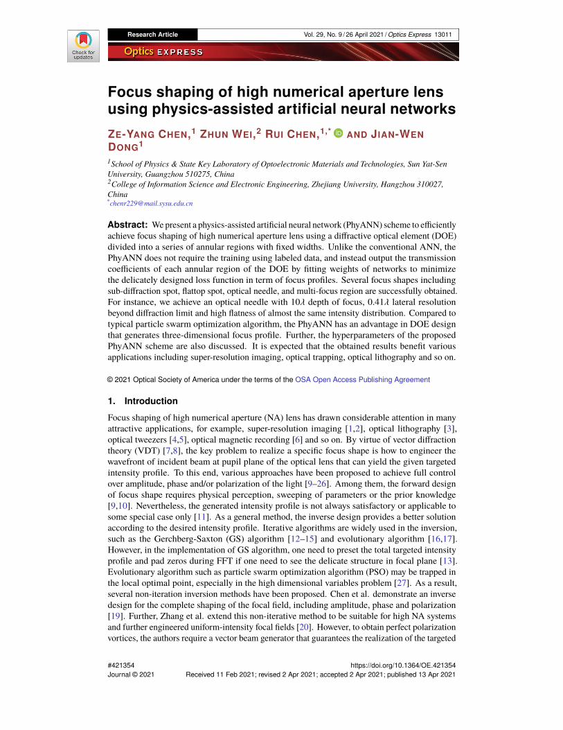
The schematic diagram of focus shaping is shown in Fig. 1. The radially polarized beam withuniform distribution is chosen as the incidence, which passes through a DOE located at the pupil

Research Article Vol. 29, No. 9 / 26 April 2021 / Optics Express 13013

plane and then focused by an aplanatic lens of high NA. Based on VDT [7,8], the radial andlongitudinal electric field components at cylindrical coordinate (r, z) around the focus can beexpressed by

Er(r, z) = A∫ θmax0 T(θ) sin(2θ)J1(kr sin θ)exp(ikz cos θ)

√cos θdθ

Ez(r, z) = 2iA∫ θmax0 T(θ)sin2(θ)J0(kr sin θ)exp(ikz cos θ)

√cos θdθ.

(1)

A is a constant and θmax is the maximum angle determined by the NA of the objective lens, givenby arcsin(NA/n), where n= 1 is the refractive index of free space. J0 and J1 are zero-order andfirst-order Bessel function of the first kind, respectively. T(θ) denotes the transmission functionof the DOE.

Fig. 1. Schematic illustration of the focusing geometry of high NA lens. (a) The radiallypolarized beam is modulated by a DOE and then focused by high NA lens. The inset iszoom in focus intensity profile. (b) The DOE with transmission coefficients, Tn, of eachannular zone.

Here, we set the DOE to be circular symmetry and θmax is divided into N equal parts, whichcorresponds to annular regions of the DOE in Fig. 1(b). The boundaries of the various region aregiven by θn, n= 1,2,. . . N, and thus the transmission function T(θ) is given by

T(θ) = Tn, θn−1 ≤ θ ≤ θn, − 1 ≤ Tn ≤ 1, n = 1, 2, . . . , N (2)

where the phase of each annular zone is set with binary value of 0 or π for different ranges ofangle θ. Consequently, the total electric field at cylindrical coordinate (r, z) (Er(r,z) or Ez(r,z)) isregarded as the linear combination of the electric field contributed by each annular zone withcorresponding weights of transmission coefficient Tn. We adopt Ern(r,z) and Ezn(r,z) to representthe contribution of the nth annular zone to the radial and longitudinal electric field components,respectively, which are determined by

Ern(r, z) = Aθn∫

θn−1

sin(2θ)J1(kr sin θ)exp(ikz cos θ)√

cos θdθ

Ezn(r, z) = 2iAθn∫

θn−1

sin2(θ)J0(kr sin θ)exp(ikz cos θ)√

cos θdθ. (3)

Research Article Vol. 29, No. 9 / 26 April 2021 / Optics Express 13014

With these equations, the total intensity at cylindrical coordinate (r, z) in the focal region can bewritten as

I(r, z) = |Er(r, z)|2 + |Ez(r, z)|2 =

|︁|︁|︁|︁|︁ N∑︂n=1

TnErn(r, z)

|︁|︁|︁|︁|︁2 +|︁|︁|︁|︁|︁ N∑︂n=1

TnEzn(r, z)

|︁|︁|︁|︁|︁2 (4)

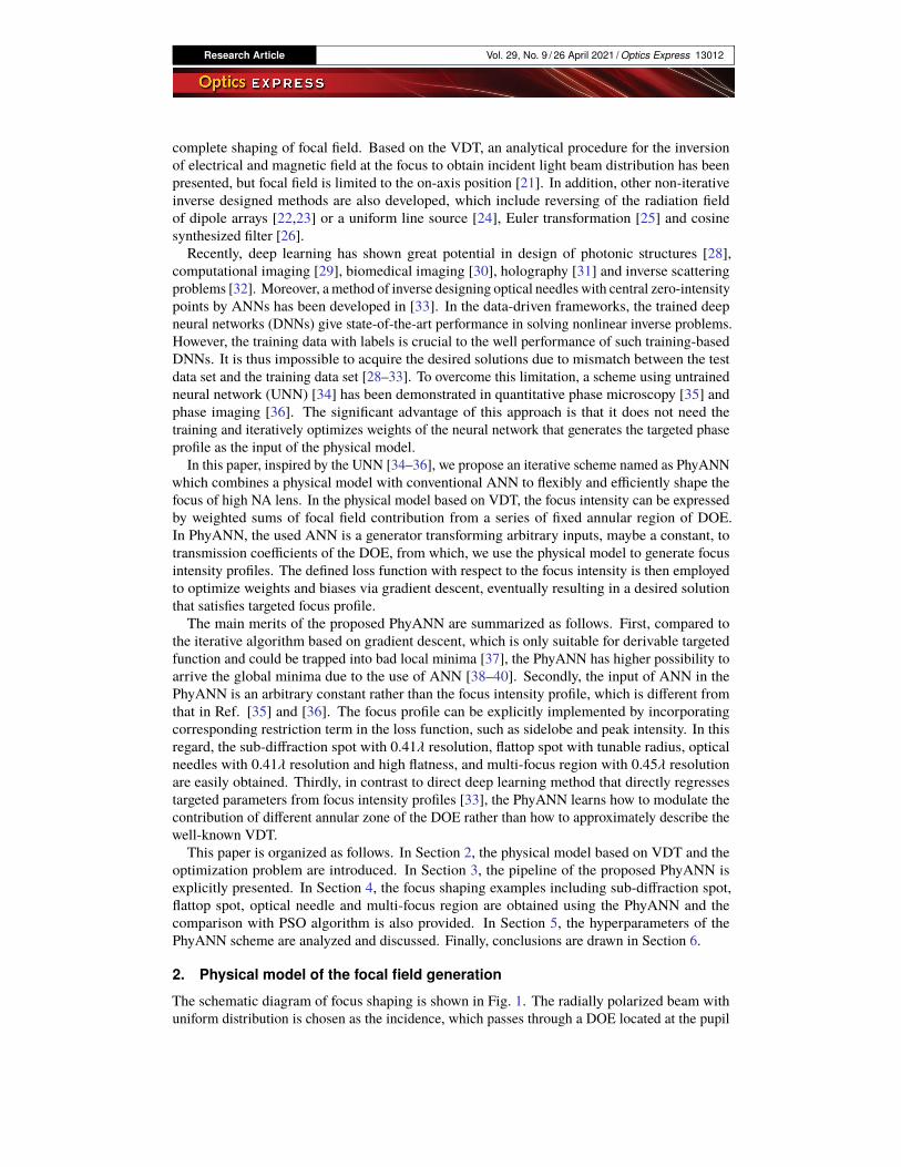
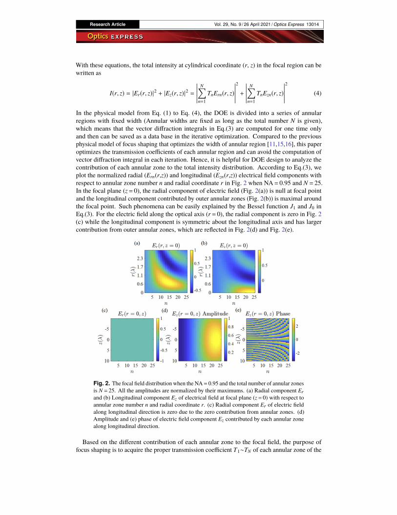
In the physical model from Eq. (1) to Eq. (4), the DOE is divided into a series of annularregions with fixed width (Annular widths are fixed as long as the total number N is given),which means that the vector diffraction integrals in Eq.(3) are computed for one time onlyand then can be saved as a data base in the iterative optimization. Compared to the previousphysical model of focus shaping that optimizes the width of annular region [11,15,16], this paperoptimizes the transmission coefficients of each annular region and can avoid the computation ofvector diffraction integral in each iteration. Hence, it is helpful for DOE design to analyze thecontribution of each annular zone to the total intensity distribution. According to Eq.(3), weplot the normalized radial (Ern(r,z)) and longitudinal (Ezn(r,z)) electrical field components withrespect to annular zone number n and radial coordinate r in Fig. 2 when NA= 0.95 and N = 25.In the focal plane (z= 0), the radial component of electric field (Fig. 2(a)) is null at focal pointand the longitudinal component contributed by outer annular zones (Fig. 2(b)) is maximal aroundthe focal point. Such phenomena can be easily explained by the Bessel function J1 and J0 inEq.(3). For the electric field along the optical axis (r= 0), the radial component is zero in Fig. 2(c) while the longitudinal component is symmetric about the longitudinal axis and has largercontribution from outer annular zones, which are reflected in Fig. 2(d) and Fig. 2(e).

Fig. 2. The focal field distribution when the NA= 0.95 and the total number of annular zonesis N = 25. All the amplitudes are normalized by their maximums. (a) Radial component Erand (b) Longitudinal component Ez of electrical field at focal plane (z= 0) with respect toannular zone number n and radial coordinate r. (c) Radial component Er of electric fieldalong longitudinal direction is zero due to the zero contribution from annular zones. (d)Amplitude and (e) phase of electric field component Ez contributed by each annular zonealong longitudinal direction.

Based on the different contribution of each annular zone to the focal field, the purpose offocus shaping is to acquire the proper transmission coefficient T1∼TN of each annular zone of the

Research Article Vol. 29, No. 9 / 26 April 2021 / Optics Express 13015

DOE, which can modulate the amplitude and phase of the incident beam to fulfill the targetedintensity I(r,z) in Eq.(4). Such process is cast into an inverse problem, which is to estimate theunknown transmission coefficient T1∼TN by minimizing the discrepancy between the computedand targeted intensity distribution:

T̃n = arg min f (Tn) (5)

where f (Tn) is a loss function, we need to define. In fact, some other optimization targets shouldbe also considered, such as side lobe and Strehl ratio (Central intensity of focal field), all ofwhich are critical parameters for the application, such as superresolution imaging and opticaltrapping. Therefore, we define the loss function as

f (Tn) =

∥︁∥︁∥︁∥︁ Ig(Tn)

Ig(r = 0, z = 0)− It

∥︁∥︁∥︁∥︁2

2+ α

[︃max

(︃ISFOV

Ig(r = 0, z = 0)

)︃− ISL

]︃2+β

SR. (6)

In the loss function, ∥ · ∥2 represents Euclidean distance and thus the first term is a fidelityterm measuring the closeness of an estimated intensity Ig to the targeted intensity. The secondterm restricts relative intensity of the maximum side lode to ISL. The third term uses Strehl Ratio(SR) as the loss function, which can maximize the intensity of the focal point, I(r= 0, z= 0). Tobe more specific, SR is defined as the ratio of the central intensity of the focal field with DOE tothat of the focal field without DOE

SR =Ig(r = 0, z = 0)

ITn=1(r = 0, z = 0). (7)

Usually the value of α and β (α>0, β > 0) is chosen empirically to balance the contribution ofcorresponding term to the total loss function. One typical method is to solve the minimizationproblem in Eq.(5) using direction optimization algorithm, for example, gradient decent method.In this work, a PhyANN scheme that combines the physical model with ANN is proposed in thefollowing. We make our implementation of PhyANN as open software in Python, which can befound at https://github.com/shepherd-cc/FocusShaping.

3. ANN-based optimization method – PhyANN

As is known to all, a typical ANN method is to optimize its weight and bias parameters usinga sufficiently large set of training data so that the ANN can represent a universal function thatmaps the transmission coefficient Tn to the targeted intensity distribution It, but it suffers fromthe limited generalization ability due to the mismatch between the test data set and the trainingdata set [33]. Such learning-based ANN method is usually considered as a black box and thustends to be more obscure [32]. Instead, a strategy to incorporate the knowledge of underlyingphysics as well as insight originated from objective function approaches into the ANN structureare the desired solution.

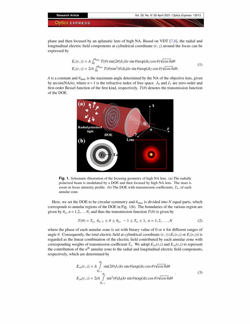
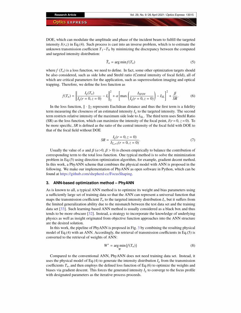
In this work, the pipeline of PhyANN is proposed in Fig. 3 by combining the resulting physicalmodel of Eq.(4) with an ANN. Accordingly, the retrieval of transmission coefficients in Eq.(5) isconverted to the retrieval of weights of ANN:

W∗ = arg minW

{f (Tn)} (8)

Compared to the conventional ANN, PhyANN does not need training data set. Instead, ituses the physical model of Eq.(4) to generate the intensity distribution Ig from the transmissioncoefficients Tn, and then employs the defined loss function of Eq.(6) to optimize the weights andbiases via gradient descent. This forces the generated intensity Ig to converge to the focus profilewith designated parameters as the iterative process proceeds.

Research Article Vol. 29, No. 9 / 26 April 2021 / Optics Express 13016

Fig. 3. The architecture of PhyANN scheme. An arbitrary constant (a unity constant here)rather than focus intensity profile is the input to the neural network. The output of the neuralnetwork is the transmission coefficients of DOE, which modulates the incident beam of thephysical model to generate the focus intensity Ig. The loss function is defined as summationof the mean square error between normalized Ig and targeted intensity It and other restrictionterm, which is employed to iteratively optimize the weights and biases via gradient descent.

The ANN used here is a generator transforming arbitrary input to transmission coefficients, Tn.Without loss of generality, a constant of c= 1 is adopted in this work. Specifically, the ANNconsists of an input layer with single neural node followed by rectified linear unit (ReLU), threehidden layers with 300 neural nodes followed by ReLU in each hidden layer and an output layerwith N neural nodes followed by activation function tanh. The number of weights can be easilytuned by changing the number of layers and the neural nodes of each layer. The weights of ANNwill be renewed with error backpropagation and gradient descent according to Eq.(8). Once theoptimal weights W are obtained when the iteration is terminated according to the targeted lossfunction, the output Tn of ANN are the optimal transmission coefficients of annular regions.

In the simulation, a normal personal computer with the configuration of CPU: Intel Corei5-9400F 3.20G and RAM:16G is used for all the computation. We use TensorFlow 2.3 andPython 3.7.7 to construct such a pipeline of PhyANN. The optimizer we used is adaptive momentestimation (Adam) [41], a stochastic gradient descent method that is based on adaptive estimationof first-order and second-order moments. We use 0.001 as the learning rate, which is a gooddefault setting for the tested machine learning problem [41].

4. Result

In the physical model, the radially polarized beam at operating wavelength 532 nm is passingthrough the DOE and focused by an aplanatic lens of NA= 0.95. Six DOEs that generate fourdifferent kinds of focus intensity profiles, including sub-diffraction spot, flattop spot, opticalneedle, and multi-focus region are inversely designed using the proposed PhyANN scheme. Forcomparison, typical PSO algorithm results are also provided [42]. It should be noted that theconvergence speed of two approaches is dependent on their hyperparameters: for example, thenumber of hidden layers and node number of each layer for the PhyANN and particle populationfor PSO.

For PSO algorithm, the particle population indeed has an important impact on the performancewhen other characteristic parameters are the default values in [42]. More specifically, theoptimization performance can be improved by increasing the particle population. However,the bigger particle population PSO algorithm chooses, the more time it takes per iteration. Tofairly compare the proposed PhyANN with PSO algorithm, we choose the proper number ofthe hidden layer (three layers) and node number of each layer (300 nodes for each layer) for

Research Article Vol. 29, No. 9 / 26 April 2021 / Optics Express 13017

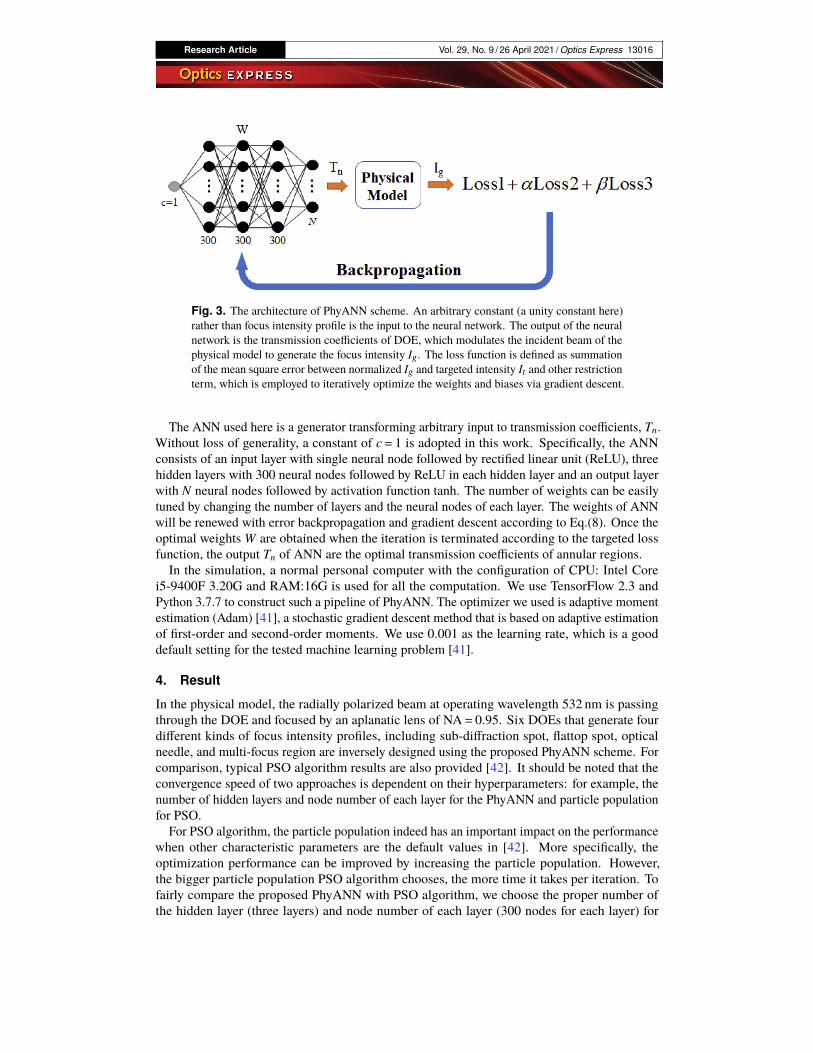
PhyANN, and obtain the DOE design results. Then, we delicately modify the particle populationof PSO algorithm to ensure that the iterations and computation time are almost same as that in theproposed PhyANN. Finally, we compare the loss function value and the SR of the focus profiles.The optimization parameters and the comparisons are provided in Table 1. It is found that forDOE designs that generate two-dimensional focus profiles (subdiffraction spots and flattop spots),the loss functions and the optimized SR are comparable for both methods. For DOE designs thatgenerate three-dimensional focus profiles (optical needles and multi-focus region), the PhyANNprovides smaller loss function value and better SR than PSO algorithm (Table 1).

Table 1. The characteristic parameters of the focus shaping examples using PhyANN and PSOalgorithm

Examples Epoch Time(s) β FWHM (λ)Loss SR

PhyANN PSO PhyANN PSO

Subdiffraction 1 200 1 1e-3 0.41 3.1e-3 3.3e-3 0.34 0.32Subdiffraction 2

(sidelobeconstraint) 500 1.9 1e-3 0.41 3.8e-3 4.1e-3 0.31 0.30

Flattop spot-1 1000 3.3 1e-4 / 3.6e-4 3.7e-4 0.28 0.28

Flattop spot-2 1000 3.3 1e-4 / 1.0e-3 1.1e-3 0.10 0.10

Optical needle 8000 23.6 1e-5 0.41 3.8e-4 6.6e-4 0.04 0.03

Multi-focus region 5000 14.8 1e-5 0.45 3.0e-4 8.0e-4 0.05 0.03

4.1. Inverse design of sub-diffraction spots

Generally, the resolution of optical microscopy is limited to 0.5λ/NA due to diffraction limit,which is described as the full width at half maximum (FWHM) of the focal spot. The sub-diffraction spot is of great importance to the resolution enhancement of optical microscopy. Toachieve the sub-diffraction spot using the proposed PhyANN scheme, two targeted intensitypoints at r= [0, FWHM/2] along radial direction with corresponding normalized intensity It = [1,0.5] is chosen in the loss function.

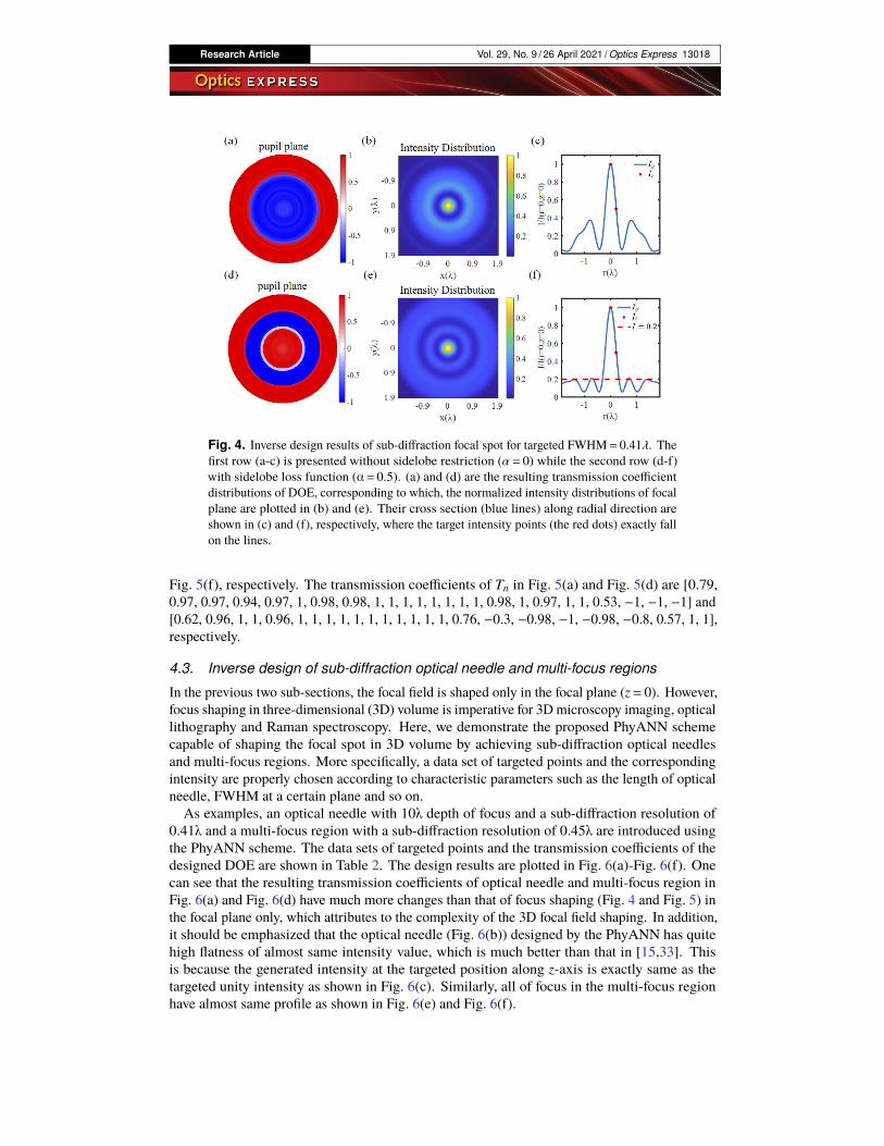
For the first case, the targeted FWHM of sub-diffraction spot is set as 0.41λ without sidelobeconstraint and the optimized transmission coefficients of Tn are obtained as shown in Fig. 4(a).The generated intensity distribution in the focal plane (calculated from the generated Tn) ispresented in Fig. 4(b). To be clear, the cross section along radial direction is also provided inFig. 4(c). It is found that two targeted intensity points (red dots in Fig. 4(c)) exactly fall on theline, proving the effectiveness and accurateness of the proposed approach. But we should notethe rising sidelobe due to the narrowing of main spot.

To alleviate the rising sidelobes, we include the sidelobe constraint in the loss function bysetting α= 0.5 and ISL = 0.2. As expected, the relative intensity of maximum sidelobe has beenrestricted to 0.2 at the expense of reduce of peak intensity of focal field, which is reflected inFig. 4(e) and Fig. 4(f). Consequently, the transmission coefficients Tn of annular regions inFig. 4(d) have a complex combination to fulfill the restriction of the sidelobe, compared to thetransmission coefficients in Fig. 4(a).

4.2. Inverse design of flattop spot

The flattop spot is attractive to many applications due to it relatively well-defined size, shapeand uniform intensity distribution, which finds application in material processing, lithographyand so on. Using the PhyANN scheme, we can easily achieve flattop spots with high flatnessand tunable radius by selecting targeted points with uniform intensity. As examples, two flattopspots with their flattop radii of 0.17λ and 0.55λ are shown in Fig. 5(a)- Fig. 5(c) and Fig. 5(d)-

Research Article Vol. 29, No. 9 / 26 April 2021 / Optics Express 13018

Fig. 4. Inverse design results of sub-diffraction focal spot for targeted FWHM= 0.41λ. Thefirst row (a-c) is presented without sidelobe restriction (α= 0) while the second row (d-f)with sidelobe loss function (α= 0.5). (a) and (d) are the resulting transmission coefficientdistributions of DOE, corresponding to which, the normalized intensity distributions of focalplane are plotted in (b) and (e). Their cross section (blue lines) along radial direction areshown in (c) and (f), respectively, where the target intensity points (the red dots) exactly fallon the lines.

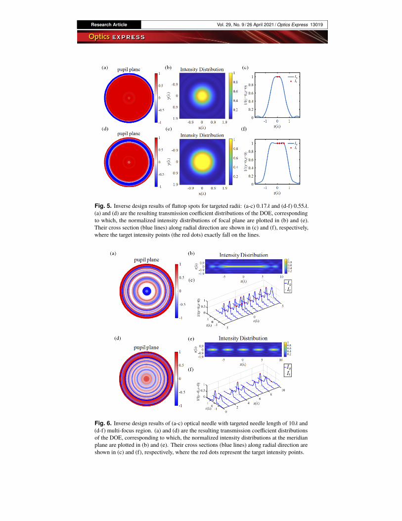
Fig. 5(f), respectively. The transmission coefficients of Tn in Fig. 5(a) and Fig. 5(d) are [0.79,0.97, 0.97, 0.94, 0.97, 1, 0.98, 0.98, 1, 1, 1, 1, 1, 1, 1, 1, 0.98, 1, 0.97, 1, 1, 0.53, −1, −1, −1] and[0.62, 0.96, 1, 1, 0.96, 1, 1, 1, 1, 1, 1, 1, 1, 1, 1, 1, 0.76, −0.3, −0.98, −1, −0.98, −0.8, 0.57, 1, 1],respectively.

4.3. Inverse design of sub-diffraction optical needle and multi-focus regions

In the previous two sub-sections, the focal field is shaped only in the focal plane (z= 0). However,focus shaping in three-dimensional (3D) volume is imperative for 3D microscopy imaging, opticallithography and Raman spectroscopy. Here, we demonstrate the proposed PhyANN schemecapable of shaping the focal spot in 3D volume by achieving sub-diffraction optical needlesand multi-focus regions. More specifically, a data set of targeted points and the correspondingintensity are properly chosen according to characteristic parameters such as the length of opticalneedle, FWHM at a certain plane and so on.

As examples, an optical needle with 10λ depth of focus and a sub-diffraction resolution of0.41λ and a multi-focus region with a sub-diffraction resolution of 0.45λ are introduced usingthe PhyANN scheme. The data sets of targeted points and the transmission coefficients of thedesigned DOE are shown in Table 2. The design results are plotted in Fig. 6(a)-Fig. 6(f). Onecan see that the resulting transmission coefficients of optical needle and multi-focus region inFig. 6(a) and Fig. 6(d) have much more changes than that of focus shaping (Fig. 4 and Fig. 5) inthe focal plane only, which attributes to the complexity of the 3D focal field shaping. In addition,it should be emphasized that the optical needle (Fig. 6(b)) designed by the PhyANN has quitehigh flatness of almost same intensity value, which is much better than that in [15,33]. Thisis because the generated intensity at the targeted position along z-axis is exactly same as thetargeted unity intensity as shown in Fig. 6(c). Similarly, all of focus in the multi-focus regionhave almost same profile as shown in Fig. 6(e) and Fig. 6(f).

Research Article Vol. 29, No. 9 / 26 April 2021 / Optics Express 13019

Fig. 5. Inverse design results of flattop spots for targeted radii: (a-c) 0.17λ and (d-f) 0.55λ.(a) and (d) are the resulting transmission coefficient distributions of the DOE, correspondingto which, the normalized intensity distributions of focal plane are plotted in (b) and (e).Their cross section (blue lines) along radial direction are shown in (c) and (f), respectively,where the target intensity points (the red dots) exactly fall on the lines.

Fig. 6. Inverse design results of (a-c) optical needle with targeted needle length of 10λ and(d-f) multi-focus region. (a) and (d) are the resulting transmission coefficient distributionsof the DOE, corresponding to which, the normalized intensity distributions at the meridianplane are plotted in (b) and (e). Their cross sections (blue lines) along radial direction areshown in (c) and (f), respectively, where the red dots represent the target intensity points.

Research Article Vol. 29, No. 9 / 26 April 2021 / Optics Express 13020

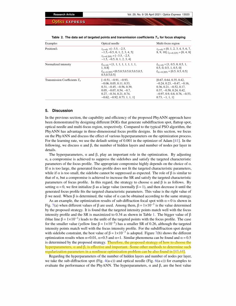
Table 2. The data set of targeted points and transmission coefficients T n for focus shaping

Examples Optical needle Multi-focus region

Position/λ z(r=0) =[−3.5, −2.5,−1.5,−0.5, 0, 1, 2, 3, 4, 5]z(r=0.205) = [−3.5, −2.5,−1.5, −0.5, 0, 1, 2, 3, 4]

z(r=0) = [0, 1, 2, 3, 4, 5, 6, 7,8, 9, 10] z(r=0.225) = [0, 4, 8]

Normalized intensity It(r=0) = [1, 1, 1, 1, 1, 1, 1, 1,1, 0.8]It(r=0.205)=[0.5,0.5,0.5,0.5,0.5,0.5,0.5,0.5,0.5]

It(r=0) = [1, 0.5, 0, 0.5, 1,0.5, 0, 0.5, 1, 0.5, 0]It(r=0.205) = [0.5, 0.5, 0.5]

Transmission Coefficients Tn [−0.51, −0.91, −0.93,−0.06, 0.05, 0.11, 0.53,0.31, −0.45, −0.56, 0.39,0.05, −0.07, 0.54, −0.7,0.27, −0.34, 0.21, 0.74,−0.62, −0.92, 0.73, 1, 1, 1]

[0.67, 0.64, 0.35, 0.42,−0.24, 0.23, −0.47, −0.16,0.36, 0.21, −0.52, 0.17,0.37, −0.58, 0.24, 0.42,−0.97, 0.9, 0.8, 0.76, −0.53,0.73, −1, 1, 1]

5. Discussion

In the previous section, the capability and efficiency of the proposed PhyANN approach havebeen demonstrated by designing different DOEs that generate subdiffraction spot, flattop spot,optical needle and multi-focus region, respectively. Compared to the typical PSO algorithm, thePhyANN has advantage in three-dimensional focus profile designs. In this section, we focuson the PhyANN and discuss the effect of various hyperparameters on the optimization process.For the learning rate, we use the default setting of 0.001 in the optimizer of Adam [41]. In thefollowing, we discuss α and β, the number of hidden layers and number of nodes per layer indetails.

The hyperparameters, α and β, play an important role in the optimization. By adjustingα, a compromise is achieved to suppress the sidelobes and satisfy the targeted characteristicparameters of the focus profile. The appropriate compromise highly depends on the choice of α.If α is too large, the generated focus profile does not fit the targeted characteristic parameters,while if α is too small, the sidelobe cannot be suppressed as expected. The role of β is similar tothat of α, but a compromise is achieved to increase the SR and satisfy the targeted characteristicparameters of focus profile. In this regard, the strategy to choose α and β is as follows. Bysetting α= 0, we first initialize β as a large value (normally β= 1), and then decrease it until thegenerated focus profile fits the targeted characteristic parameters. This value is the right value ofβ we need. When β is determined, the value of α can be obtained according to the same strategy.

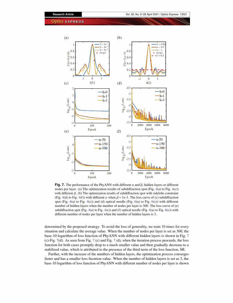
As an example, the optimization results of sub-diffraction focal spot with α= 0 is shown inFig. 7(a) when different values of β are used. Among them, β= 1×10−3 is the value determinedby the proposed strategy. It is found that the targeted intensity points match well with the focusintensity profile and the SR is maximized to 0.34 as shown in Table 1. The bigger value of β(blue line β= 1×10−1) leads to the unfit of the targeted points with the focus profile. The casefor the smaller value (yellow line β= 1×10−5) has a smaller SR of 0.26, although the targetedintensity points match well with the focus intensity profile. For the subdiffraction spot designwith sidelobe constraint, the best value of β= 1×10−3 is adopted. Figure 7(b) shows the differentoptimization results when α=0.01, α=0.5 and α=1. Similar phenomena can be found and α= 0.5is determined by the proposed strategy. Therefore, the proposed strategy of how to choose thehyperparameters, α and β, is effective and important. Some other methods to determine suchregularization parameters in a nonlinear optimization problem can be also found in [43,44].

Regarding the hyperparameters of the number of hidden layers and number of nodes per layer,we take the sub-diffraction spot (Fig. 4(a-c)) and optical needle (Fig. 6(a-c)) for examples toevaluate the performance of the PhyANN. The hyperparameters, α and β, are the best value

Research Article Vol. 29, No. 9 / 26 April 2021 / Optics Express 13021

Fig. 7. The performance of the PhyANN with different α and β, hidden layers or differentnodes per layer. (a) The optimization results of subdiffraction spot (Fig. 4(a) to Fig. 4(c))with different β. (b) The optimization results of subdiffraction spot with sidelobe constraint(Fig. 4(d) to Fig. 4(f)) with different α when β= 1e-3. The loss curve of (c) subdiffractionspot (Fig. 4(a) to Fig. 4(c)) and (d) optical needle (Fig. 6(a) to Fig. 6(c)) with differentnumber of hidden layers when the number of nodes per layer is 300. The loss curve of (e)subdiffraction spot (Fig. 4(a) to Fig. 4(c)) and (f) optical needle (Fig. 6(a) to Fig. 6(c)) withdifferent number of nodes per layer when the number of hidden layers is 3.

determined by the proposed strategy. To avoid the loss of generality, we train 10 times for everysituation and calculate the average value. When the number of nodes per layer is set as 300, thebase-10 logarithm of loss function of PhyANN with different hidden layers is shown in Fig. 7(c)-Fig. 7(d). As seen from Fig. 7 (c) and Fig. 7 (d), when the iteration process proceeds, the lossfunction for both cases promptly drop to a much smaller value and then gradually decrease to astabilized value, which is attributed to the presence of the third term of the loss function, SR.

Further, with the increase of the numbers of hidden layers, the optimization process convergesfaster and has a smaller loss fucntion value. When the number of hidden layers is set as 3, thebase-10 logarithm of loss function of PhyANN with different number of nodes per layer is shown

Research Article Vol. 29, No. 9 / 26 April 2021 / Optics Express 13022

in Fig. 7(e)-Fig. 7(f). It is also found that the optimization process converges fast at beginning andthen go to a steady state. However, there is not much improvement when we increase numbers ofnodes per layer. To sum up, more hidden layers or nodes per layers indicate better performance inthe optimization. However, in practical, we should note that the more layers or nodes means theincreasing computation cost. Therefore, we should make a tradeoff between computational costand optimization performance according to the complexity of the problem we need to resolve.

6. Conclusion

In this work, we present an ANN-based iterative scheme, named as PhyANN, for DOE design toshape focus of a high NA objective lens. In contrast to the conventional ANN that requires atraining process, the PhyANN reconstructs the DOE by combining a conventional ANN with aphysical model of VDT that generates focus intensity profiles from the transmission function ofthe DOE. The defined loss function with respect to the focus intensity profile is employed tooptimize weights and biases via gradient descent, eventually resulting in a desired solution thatsatisfies targeted focus profiles.

By delicately designing the loss function and then feedback to the ANNs, we achieve asub-diffraction focal spot of FWHM= 0.41λ with the intensity of maximum sidelobe less thanone fifth of the peak intensity. Flattop spots with different size are easily obtained by increasingthe target points with unit intensity. Meanwhile, the proposed scheme shows the high freedom toshape the focus in 3D volume by achieving a sub-diffraction optical needle with a 10λ depthof focus and 0.41λ beyond diffraction limit resolution. A multi-focus region along longitudinalaxis with lateral resolution of 0.45λ is also obtained. It should be mentioned that we canefficiently achieve the focus profile with the targeted characteristic parameters from second totens of seconds. This is attributed to the architecture of the proposed PhyANN that incorporatesknowledge of the underlying physics and insight originated from the designed loss function.

In the physical model based on VDT, the amplitude and phase hybrid modulation DOE isadopted and is divided into a series of annular regions with fixed widths, which allows us tooptimize the transmission coefficients instead of the annular widths that is normally used inbibliography [11–17]. As a result, the vector diffraction integral of Eq. (3) is computed forone time only and then can be saved as a data base. Further, the amplitude and phase hybridmodulation DOE means the extension of the degree of the freedom for generation of focus profiles.However, we should also note the implementation of the amplitude and phase hybrid modulationDOE is a little bit complicated than common phase-only case. Fortunately, some amplitudeand phase hybrid modulation DOEs have been developed [45] and the emerging metasurfacedevices can also provide both amplitude and phase modulation of light beam in subwavelengthscale using the prescribed nanostructures [16,46]. Therefore, it will not be a problem for theexperimental implementation.

In addition, we have compared the proposed PhyANN with the typical PSO Algorithm. It isfound that for DOE designs that generate the two-dimensional focus profiles (subdiffraction spotsand flattop spots), the loss functions and the optimized SR are comparable for both methods whenthe almost the same computation time and iterations are set in the optimization process. For DOEdesigns that generate three-dimensional focus profiles (optical needle and multi-focus region),the PhyANN provides slightly better loss function value and better SR than PSO algorithm. Itcan be concluded that the proposed PhyANN can offer an alternative method to effectively designthe annular pupil filter that generates the targeted focus profile. Such study provides not onlyan interesting opportunity for many applications such as super-resolution microscopy, opticaltweezers, optical lithography and optical storage, but also a promising direction that combiningunderlying physics with ANN to solve nonlinear inverse problems.Funding. National Natural Science Foundation of China (61905291, 61805288); Guangdong Basic and Applied Basic

Research Article Vol. 29, No. 9 / 26 April 2021 / Optics Express 13023

Research Foundation (2020A1515010626); The Open Project Program of Wuhan National Laboratory for Optoelectronics(2019WNLOKF020); Fundamental Research Funds for the Central Universities (19lgpy271).

Disclosures. The authors declare no conflicts of interest.

Data availability. Data underlying the results presented in this paper are not publicly available at this time but maybe obtained from the authors upon reasonable request.

References1. R. Schmidt, C. A. Wurm, S. Jakobs, J. Engelhardt, A. Egner, and S. W. Hell, “Spherical nanosized focal spot unravels

the interior of cells,” Nat. Methods 5(6), 539–544 (2008).2. E. L. Loh, R. Chen, K. Agarwal, and X. Chen, “Feature-based filter design for resolution enhancement of known

features in microscopy,” J. Opt. Soc. Am. A 31(12), 2610–2617 (2014).3. Z. Gan, Y. Cao, R. A. Evans, and M. Gu, “Three-dimensional deep sub-diffraction optical beam lithography with

9 nm feature size,” Nat. Commun. 4(1), 2061 (2013).4. D. McGloin and J. P. Reid, “Forty years of optical manipulation,” Opt. Photonics News 21(3), 20 (2010).5. M. E. J. Friese, T. A. Nieminen, N. R. Heckenberg, and H. Rubinsztein-Dunlop, “Optical alignment and spinning of

laser-trapped microscopic particles,” Nature 394(6691), 348–350 (1998).6. Y. Jiang, X. Li, and M. Gu, “Generation of sub-diffraction-limited pure longitudinal magnetization by the inverse

Faraday effect by tightly focusing an azimuthally polarized vortex beam,” Opt. Lett. 38(16), 2957–2960 (2013).7. E. Wolf, “Electromagnetic diffraction in optical systems .I. an integral representation of the image field,” Proc. R.

Soc. Lond. A 253(1274), 349–357 (1959).8. K. S. Youngworth and T. G. Brown, “Focusing of high numerical aperture cylindrical-vector beams,” Opt. Express

7(2), 77–87 (2000).9. C. J. R. Sheppard, J. Campos, J. Escalera, and S. Ledesma, “Two-zone pupil filters,” Opt. Commun. 281(5), 913–922

(2008).10. C. J. R. Sheppard and A. Choudhury, “Annular pupils, radial polarization, and superresolution,” Appl. Opt. 43(22),

4322–4327 (2004).11. X. Hao, C. Kuang, T. Wang, and X. Liu, “Phase encoding for sharper focus of the azimuthally polarized beam,” Opt.

Lett. 35(23), 3928–3930 (2010).12. R. Gerchberg and A. Saxton, “A practical algorithm for the determination of phase from image and diffraction plane

pictures,” Optik 35, 237–250 (1971).13. K. Jahn and N. Bokor, “Intensity control of the focal spot by vectorial beam shaping,” Opt. Commun. 283(24),

4859–4865 (2010).14. J. Hao, Z. Yu, H. Chen, Z. Chen, H. Wang, and J. Ding, “Light field shaping by tailoring both phase and polarization,”

Appl. Opt. 53(4), 785–791 (2014).15. H. M. Guo, X. Y. Weng, M. Jiang, Y. H. Zhao, G. R. Sui, Q. Hu, Y. Wang, and S. L. Zhuang, “Tight focusing of a

higher-order radially polarized beam transmitting through multi-zone binary phase pupil filters,” Opt. Express 21(5),5363–5372 (2013).

16. Z. Zhuang, R. Chen, Z. Fan, X. Pang, and J. Dong, “High focusing efficiency in subdiffraction focusing metalens”,”Nanophotonics 8(7), 1279–1289 (2019).

17. J. Lin, H. Zhao, Y. Ma, J. Tan, and P. Jin, “New hybrid genetic particle swarm optimization algorithm to designmulti-zone binary filter,” Opt. Express 24(10), 10748–10758 (2016).

18. Y. Zhao, Q. Zhan, and Y. P. Li, “Design of DOE for beam shaping with highly NA focused cylindrical vector beam,”Proc. SPIE 5636, 56 (2005).

19. Z. Chen, T. Zeng, and J. Ding, “Reverse engineering approach to focus shaping,” Opt. Lett. 41(9), 1929–1932 (2016).20. G. Zhang, X. Gao, Y. Pan, M. Zhao, D. Wang, H. Zhang, Y. Li, C. Tu, and H. Wang, “Inverse method to engineer

uniform-intensity focal fields with arbitrary shape,” Opt. Express 26(13), 16782–16796 (2018).21. J. Borne, D. Panneton, M. Piche, and S. Thibault, “Analytical inversion of the focusing of high-numerical-aperture

aplanatic systems,” J. Opt. Soc. Am. A 36(10), 1642–1647 (2019).22. J. Wang, W. Chen, and Q. Zhan, “Engineering of high purity ultra-long optical needle field through reversing the

electric dipole array radiation,” Opt. Express 18(21), 21965–21972 (2010).23. J. Wang, W. Chen, and Q. Zhan, “Three-dimensional focus engineering using dipole array radiation pattern,” Opt.

Commun. 284(12), 2668–2671 (2011).24. Y. Yu and Q. Zhan, “Optimization-free optical focal field engineering through reversing the radiation pattern from a

uniform line source,” Opt. Express 23(6), 7527–7534 (2015).25. J. Lin, K. Yin, Y. Li, and J. Tan, “Achievement of longitudinally polarized focusing with long focal depth by amplitude

modulation,” Opt. Lett. 36(7), 1185–1187 (2011).26. T. Liu, J. B. Tan, J. Liu, and J. Lin, “Creation of subwavelength light needle, equidistant multi-focus, and uniform

light tunnel,” J. Mod. Opt. 60(5), 378–381 (2013).27. J. J. Jamian, M. N. Abdullah, H. Mokhlis, M. W. Mustafa, and A. H. A. Bakar, “Global Particle Swarm Optimization

for High Dimension Numerical Functions Analysis,” Journal of Applied Mathematics 2014, 1–14 (2014).28. W. Ma, Z. Liu, and Z. A. Kudyshev, “Deep learning for the design of photonic structures,” Nat. Photonics. 15, 77–90

(2021).

Research Article Vol. 29, No. 9 / 26 April 2021 / Optics Express 13024

29. A. Sinha, J. Lee, S. Li, and G. Barbastathis, “Lensless computational imaging through deep learning,” Optica 4(9),1117–1125 (2017).

30. Z. Zong, Y. Wang, and Z. Wei, “A Review of Algorithms and Hardware Implementations in Electrical ImpedanceTomography (Invited),” Prog. Electromagn. Res. 169, 59–71 (2020).

31. Y. Rivenson, Y. Zhang, H. Günaydın, D. Teng, and A. Ozcan, “Phase recovery and holographic image reconstructionusing deep learning in neural networks,” Light: Sci. Appl. 7(2), 17141 (2018).

32. Z. Wei and X. Chen, “Physics-Inspired Convolutional Neural Network for Solving Full-Wave Inverse ScatteringProblems,” IEEE Trans. Antennas Propag. 67(9), 6138–6148 (2019).

33. W. Xin, Q. Zhang, and M. Gu, “Inverse design of optical needles with central zero-intensity points by artificial neuralnetworks,” Opt. Express 28(26), 38718–38732 (2020).

34. V. Lempitsky, A. Vedaldi, and D. Ulyanov, “Deep Image Prior,” in 2018 IEEE/CVF Conference on Computer Visionand Pattern Recognition, 2018, 9446–9454.

35. E. Bostan, R. Heckel, M. Chen, M. Kellman, and L. Waller, “Deep phase decoder: self-calibrating phase microscopywith an untrained deep neural network,” Optica 7(6), 559–562 (2020).

36. F. Wang, Y. Bian, H. Wang, M. Lyu, G. Pedrini, W. Osten, G. Barbastathis, and G. Situ, “Phase imaging with anuntrained neural network,” Light: Sci. Appl. 9(1), 77 (2020).

37. M. M. Noel, “A new gradient based particle swarm optimization algorithm for accurate computation of globalminimum,” Appl. Soft Comput. 12(1), 353–359 (2012).

38. A. Choromanska, M. Henaff, M. Mathieu, G. B. Arous, and Y. LeCun, “The loss surfaces of multilayer networks,”Proc. Artificial Intelligence and Statistics 192–204 (2015).

39. B. D. Haeffele and R. Vidal, “Global optimality in neural network training,” Proc. IEEE Conf. Computer Vision andPattern Recognition, 4390–4398 (2017).

40. S. S. Du, J. D. Lee, H. Li, L. Wang, and X. Zhai, Gradient descent finds global minima of deep neural networks(2018). arXiv:1811.03804

41. D. Kingma and J. Ba, et al. Adam: a method for stochastic optimization. Preprint at https://arxiv.org/abs/1412.6980(2014).

42. B. Birge, “PSOt - a particle swarm optimization toolbox for use with Matlab,” in Proceedings of the 2003 IEEESwarm Intelligence Symposium. SIS’03 (Cat. No.03EX706), 2003, 182–186.

43. Y. W. Wen and R. H. Chan, “Parameter selection for total-variation based image restoration using discrepancyprinciple,” IEEE Trans. on Image Process. 21(4), 1770–1781 (2012).

44. G. M. P. van Kempen and L. J. van Vliet, “The influence of the regularization parameter and the first estimate on theperformance of Tikhonov regularized non-linear image restoration algorithms,” J. Microsc. 198(1), 63–75 (2000).

45. Hwi Kim and Byoungho Lee “Phase and amplitude modulation of a two-dimensional subwavelength diffractiveoptical element on artificial distributed-index medium”, Proc. SPIE 4929, Optical Information Processing Technology,(16 September 2002);

46. N. Yu and F. Capasso, “Flat optics with designer metasurfaces,” Nat. Mater. 13(2), 139–150 (2014).