Embed Size (px)
Citation preview
An Aperture Synthesis Technique for Cylindrical Printed
Lens / Transmitarray Antennas with Shaped Beams
by
Mahmud Biswas
A thesis submitted to the
Faculty of Graduate and Postdoctoral Studies
in partial fulfillment of the requirements for the degree of
Master of Applied Science
in Electrical & Computer Engineering
Ottawa-Carleton Institute for Electrical and Computer Engineering
School of Electrical Engineering and Computer Science
Faculty of Engineering
University of Ottawa
©Mahmud Biswas,Ottawa,Canada,2013

1
ABSTRACT
Printed lens antennas offer the possibility of realizing shaped beam patterns using no more
complexity than is required for pencil beam patterns. Shaped beam patterns can be obtained by
appropriately determining the complex transmission coefficient required for each cell (or
element) of the printed lens, taking into account the varying feed field over the input surface of
the lens. Certain ranges of transmission coefficient amplitude and phase are undesirable (eg. too
low an amplitude implies a large reflection at the lens input surface). It would be preferable to
constrain the range of values that the transmission coefficient can take as an integral part of the
lens synthesis procedure, and thus the transmission coefficient itself needs to be the synthesis
variable. In this thesis a synthesis technique for doing this is developed based on the method of
generalized projections, modified to “operate” in the space of transmission coefficients. This
makes it possible to immediately perceive what influence constraints on the actual transmission
coefficients have on the possible radiation pattern performance. In addition, an approach that
allows one to constrain the transmission coefficient to values that must be selected from an
available database of transmission coefficients is incorporated into the synthesis technique.
Keywords:
Printed lens, transmitarray, aperture synthesis, shaped beams

2
ACKNOWLEDGEMENTS
I am very grateful for the guidance and support of my supervisor Dr. Derek McNamara, who
kindly agreed to take me on when, mid-stream in my masters degree studies, my technical
interests shifted to the antenna field. I am especially grateful for his allowing me to liberally
garner material from his notes on array synthesis for the literature review in Chapter 2. I am
extremely indebted to him for his personal attention and patience in meticulously sketching out
the map of the research studies. Without his unwavering support and encouragement, this thesis
wouldn’t have come to a successful completion. One simply could not wish for a better or
friendlier supervisor.
I would also like to thank the past and present members of the Antenna Research Group at the
School of Electrical Engineering & Computer Science of the University of Ottawa. Special
thanks go to Dr. Nicolas Gagnon of the Communication Research Centre Canada for permitting
me to use his phase-shifting surface database in describing the “opportunistic” synthesis method.
A special appreciation goes to my colleague Mr. Mohan Bhardwaj at the Department of National
Defence for his constant moral support and encouragement throughout this research work.
.
Last but not least, I would like to pay high regards to my parents and my sister for their sincere
encouragement and inspiration throughout my research work and lifting me uphill during this
phase of life. I owe everything to them.
3
TABLE OF CONTENTS
CHAPTER 1
Introduction
1.1 SHAPED BEAM ANTENNAS …………………………………………………………6
1.2 PRINTED LENS / TRANSMITARRAY ANTENNAS ………………………………..7
1.3 THE CONSTRAINED ARRAY ELEMENT EXCITATION SYNTHESIS
PROBLEM ………………………………………………………………………………13
1.4 OVERVIEW OF THE THESIS …………………………………………………………15
1.5 REFERENCES FOR CHAPTER 1………………………………………………………16
CHAPTER 2
Review of Array Antenna Excitation Synthesis Techniques
2.1 INTRODUCTION……………………………………………………………………… 19
2.2 ARRAY PATTERN ANALYSIS EXPRESSIONS …………………………………… 20
2.3 PRINTED LENS / TRANSMITARRAY ANTENNA DESIGN AS AN ARRAY
EXCITATION SYNTHESIS PROBLEM………………………………………………26
2.4 CLASSICAL EXCITATION SYNTHESIS TECHNIQUES & THEIR
LIMITATIONS………………………………………………………………………….31
2.5 SYNTHESIS METHODS DIRECTLY BASED ON CONVENTIONAL NUMERICAL
OPTIMISATION
ALGORITHMS…………………………………………………………………………41
2.6 SYNTHESIS METHODS BASED ON CONVEX PROGRAMMING
ALGORITHMS…………………………………………………………………………45
4
2.7 EXCITATION SYNTHESIS USING THE METHOD OF GENERALIZED
PROJECTIONS………………………………………………………………………….46
2.8 SELECTION OF STARTING POINTS FOR NUMERICAL SYNTHESIS
METHODS………………………………………………………………………………59
2.9 SHAPED BEAM PATTERN MASKS………………………………………………….60
2.10 CONCLUSIONS………………………………………………………………………..70
2.11 REFERENCES FOR CHAPTER 2 …………………………………………………….78
CHAPTER 3
Modified Method of Projections for Transmission
Coefficient Synthesis of Cylindrical Printed Lens Antennas
3.1 GOALS………………………………………………………………………………...84
3.2 MODEL FOR THE NORMALIZED FEED FIELD ( )in
y nE x ………………………….85
3.3 FORWARD OPERATOR WITH LENS ELEMENT TRANSMISSION COEFFICIENTS
AS SYNTHESIS VARIABLES………………………………………………………87
3.4 REVERSE OPERATOR WITH LENS ELEMENT TRANSMISSION COEFFICIENTS
AS SYNTHESIS VARIABLES……………………………………………………….89
3.5 PROJECTION OPERATORS FOR TRANSMISSION COEFFICIENT AMPLITUDE
DYNAMIC RANGE RESTRICTIONS………………………….90
3.6 PROJECTION OPERATORS FOR TRANSMISSION COEFFICIENT AMPLITUDE &
PHASE RESTRICTIONS……………………………………………………………..93
3.7 PROJECTION OPERATORS FOR PHASE-ONLY SYNTHESIS………………….94
3.8 PROJECTION OPERATOR FOR TRANSMISSION COEFFICIENT CONSTRAINTS
SUBJECT TO MEMBERSHIP OF A RESTRICTED DATABASE………………….96
3.9 PROJECTION ALGORITHMS WITH PATTERN AND TRANSMISSION
COEFFICIENT CONSTRAINTS……………………………………………………..97
5
3.10 STARTING VALUE ESTIMATION OF THE EXCITATION PHASES FOR
PROJECTION SYNTHESIS OF SHAPED BEAM PATTERNS……………………99
3.11 CONCLUDING REMARKS…………………………………………………………….111
3.12 REFERENCES FOR CHAPTER 3……………………………………………………112
CHAPTER 4
Application of the Constrained Transmission Coefficient
Synthesis Methods to Shaped Beam Problems
4.1 PRELIMINARY REMARKS…………………………………………………………113
4.2 FLAT-TOPPED PATTERN SYNTHESIS……………………………………………114
4.3 ISOFLUX PATTERN SYNTHESIS…………………………………………………..133
4.4 COSECANT PATTERN SYNTHESIS……………………………………………….135
4.5 CONCLUDING REMARKS………………………………………………………….141
4.6 REFERENCES FOR CHAPTER 4……………………………………………………142
CHAPTER 5
General Conclusions……………………………………………………………143
6
List of Figures
1.1-1 Shaped beam radiation patterns compared to conventional pencil beam case .......………..9
1.1-2 Illustration of printed transmitarray antenna configuration………………………………..10
1.1-3 Side view of the horn-fed transmitarray antenna, for the case of a
four-conducting-layer printed surface (After [30]) …………….……………….…….…..11
1.1-3 Quantized output aperture of the transmitarray antenna…………………………………..11
2.2-1 Illustration of the rotational symmetry of the array factor of a linear array…………….…23
2.2-2 Element numbering schemes for arrays with an even and odd number of elements……...24
2.2-3 Element numbering schemes for symmetric arrays ……………………..……………...…25
2.3-1 Cross-section through cylindrical printed lens…………………………………………….28
2.4-1 Graph of Chebyshev polynomial ……………………………………………………..…...34
2.4-2 Enlargement of a portion of the graph of polynomial from Fig 2.4-1, and
quantities related to Chebyshev array synthesis ………………….…………….…….…...35
2.7-1 Excitation and pattern spaces in terms of which the method of
generalized projections is defined (Courtesy of D. A. McNamara) …………..….……….55
2.9-1 Idealized pencil beam gain pattern ……………………………………………………..…61
2.9-2 Pattern specification mask for use in the synthesis of pencil beam patterns ……………...62
2.9-3 Idealized flat-topped (sector) beam gain pattern …………………………..….….…….…63
2.9-4 Idealized flat-topped (sector) beam pattern ………………………………………..……...64
2.9-5 Sketch Illustrating Satellite-Earth Geometry for Derivation of the Shaped Pattern
Characteristics Required for an Isoflux Antenna……………………… …………………65
2.9-6 (a) Idealised directivity patterns for satellite orbital height 8000km and (b) 800 km …….68
2.9-7 Pattern mask for isoflux pattern ……………………………………………..……. .…….69
2.9-8 Surveillance radar antenna and approaching aircraft ………………………..…….……..71
2.9-9 Idealized cosecant pattern for ground-based surveillance radar antenna …………...……72
7
2.9-10 Depiction of a base station antenna, and users at various distances from it,
in wireless network cell ………………………………………………………….….…74
2.9-11 Idealized cosecant pattern for base-station antenna of wireless network cell…….……74
2.9-12 Masks for cosecant pattern ……………………………………………………..…..…76
3.2-1 Relationship between the feed model and printed lens geometries ……………..………85
3.6-1 Illustration of the Amplitude and Phase Constraint Restriction Operator……..……...…94
3.10-1 Starting Phase of the Excitations for a Flat-Topped Beam Pattern…………………...104
3.10-2 Radiation Pattern Using the Excitation Starting Phase Values in Fig. 3.10-1………...105
3.10-3 Starting Phase of the Excitations for an Isoflux Beam Pattern………………………..107
3.10-4 Radiation Pattern Using the Excitation Starting Phase Values in Fig. 3.10-3……..….108
3.10-5 Starting Phase of the Excitations for a Cosecant Beam Pattern………………………110
3.10-6 Radiation Pattern Using the Excitation Starting Phase Values in Fig. 3.10-5……...…111
4.2-1 Synthesized Flat-Topped Beam Pattern
(No Transmission Coefficient Constraints) with Ne =32………………………………...115
4.2-2 SDE for Synthesized Flat-Topped Beam Pattern
(No Transmission Coefficient Constraints) with Ne =32……………………..……….....115
4.2-3 Transmission Coefficients Amplitudes of the Synthesized Flat-Topped
Beam Pattern (No Transmission Coefficient Constraints) with Ne =32………….……....116
4.2-4 Transmission Coefficients Phases of the Synthesized Flat-Topped
Beam Pattern (No Transmission Coefficient Constraints) with Ne =32…………….........116
4.2-5 Synthesized Flat-Topped Beam Pattern
(No Transmission Coefficient Constraints) with Ne =24………………………………...117
4.2-6 Synthesized Flat-Topped Beam Pattern
(No Transmission Coefficient Constraints) with Ne =40……………………..………….118
4.2-7 Synthesized Flat-Topped Beam Pattern (Transmission Coefficient
Amplitude Constrained to be Larger Than -1dB with Ne =32…………………………...119
4.2-8 SDE for Synthesized Flat-Topped Beam Pattern (Transmission
Coefficient Amplitude Constrained to be Larger Than -1dB with Ne =32…….………...120
8
4.2-9 Transmission Coefficients Amplitudes of the Synthesized
Flat-Topped Beam (Transmission Coefficient Amplitude Constrained
to be Larger Than -1dB) with Ne =32…………………………………………………120
4.2-10 Transmission Coefficients Phases of the Synthesized Flat-Topped Beam (Transmission
Coefficient Amplitude Constrained to be Larger Than -1dB) with Ne =32………….121
4.2-11 Synthesized Flat-Topped Beam Pattern (Transmission Coefficient
Amplitude Constrained to be Larger Than -3dB with Ne =32………………………...121
4.2-12 Transmission Coefficients Amplitudes of the Synthesized
Flat-Topped Beam Pattern (Transmission Coefficient Amplitude
Constrained to be Larger Than -3dB with Ne =32………………………………….....122
4.2-13 Synthesized Flat-Topped Beam Pattern (Transmission Coefficient Amplitude
Constrained to be Larger Than -1dB with Ne =40…………………………………….122
4.2-14 Synthesized Flat-Topped Beam Pattern (Transmission Coefficient
Amplitude Constrained to be Larger Than -3dB with Ne =24………………………...123
4.2-15 Synthesized Flat-Topped Beam Pattern (Phase-Only Constraint) with Ne =32……....124
4.2-16 SDE for Flat-Topped Beam Synthesis (Phase-Only Constraint) with Ne =32………...125
4.2-17 Synthesized Flat-Topped Beam Transmission Coefficient
Amplitudes (Phase-Only Constraint) with Ne =32………………………………........125
4.2-18 Synthesized Flat-Topped Beam Transmission Coefficient
Phase (Phase-Only Constraint) with Ne =32……………………………………….….126
4.2-19 Synthesized Flat-Topped Beam Pattern (Phase-Only
Constraint) with Ne =32 and Srip increased form 1 dB to 2dB……………………….126
4.2-20 SDE for Synthesized Flat-Topped Beam Pattern
(Phase-Only Constraint) with Ne =32 and Srip increased form 1 dB to 2dB………....127
4.2-21 Synthesized Flat-Topped Beam Pattern (Transmission
Coefficient Amplitude Constrained o be Larger Than -1dB) with Ne =32…….…...127
4.2-22 Database of Lens Element Transmission Coefficients…………………………..….....129
4.2-23 Synthesized Flat-Topped Beam for Transmission Coefficients
Constrained to be Members of the Database in Fig. 4.2-22 (with Ne =32)…….……..130
4.2-24 Synthesized Flat-Topped Beam Transmission Coefficient
Phases for the Pattern in Fig. 4.2-23 (with Ne =32)…………………………….....…..130
9
4.2-25 Synthesized Flat-Topped Beam Transmission Coefficient
Amplitudes for the Pattern in Fig. 4.2-23 (with Ne =32)…………………….…….....131
4.2-26 Database of Lens Element Transmission Coefficients,
Restricted to Transmission Coefficient Greater Than -2dB………………………......131
4.2-27 Synthesized Flat-Topped Beam Pattern for Transmission Coefficients
Constrained to be Members of the Database in Fig. 4.2-26 (with = Ne 32)…………..132
4.2-28 Synthesized Flat-Topped Beam Transmission Coefficients
Phases for the Pattern in Fig. 4.2-27 (with Ne =32)…………………………………..132
4.2-29 Synthesized Flat-Topped Beam Transmission Coefficients
Amplitudes for the Pattern in Fig. 4.2-27 (with Ne =32)………………………….…..133
4.3-1 Synthesized Isoflux Beam Pattern (No Transmission
Coefficient Constraints) with = Ne 32………………………………………………...134
4.3-2 Synthesized Isoflux Beam Pattern (Phase-Only Constraints) with Ne =32…….……....134
4.3-3 Synthesized Isoflux Beam Pattern (Dynamic Range
Constraints 2 0ndB b dB ) with Ne =32……………………………………...…..135
4.4-1 Synthesized Cosecant Beam Pattern (No Transmission
Coefficient Constraints) with Ne =32……………………………………….………...137
4.4-2 Transmission Coefficient Amplitude for the Pattern in Fig. 4.4-1…...137
4.4-3 Transmission Coefficient Phase for the Pattern in Fig. 4.4-1…………………………..138
4.4-4 Synthesized Cosecant Beam Pattern (Transmission Coefficient
Phase Range Constraint -130 130 130nb o o ) with Ne =32………………...…....138
4.4-5 Transmission Coefficient Phase for the Pattern in Fig. 4.4-4…………………………..139
4.4-6 Synthesized Cosecant Beam Pattern with Pattern Mask Parameters
Tightened to (No Transmission Coefficient Constraints) with Ne =32…………...…..139
4.4-7 Cosecant Beam Pattern from a Phase-Only Synthesis Using
the Serial Form of the Projection Algorithm with Ne =32………………………….....140
4.4-8 Cosecant Beam Pattern from a Phase-Only Synthesis Using the Parallel Form
of the Projection Algorithm with 1 0.8 and 2 0.2 , and Ne = 32……………….140
4.4-9 Synthesized Transmission Coefficients Amplitudes for the Pattern in Fig. 4.4-8 …….141
10
CHAPTER 1 Introduction
1.1 SHAPED BEAM ANTENNAS
The need for antennas with shaped beam, as opposed to pencil beam, patterns arises in many
applications, including satellite communications, terrestrial wireless networks, and radar systems
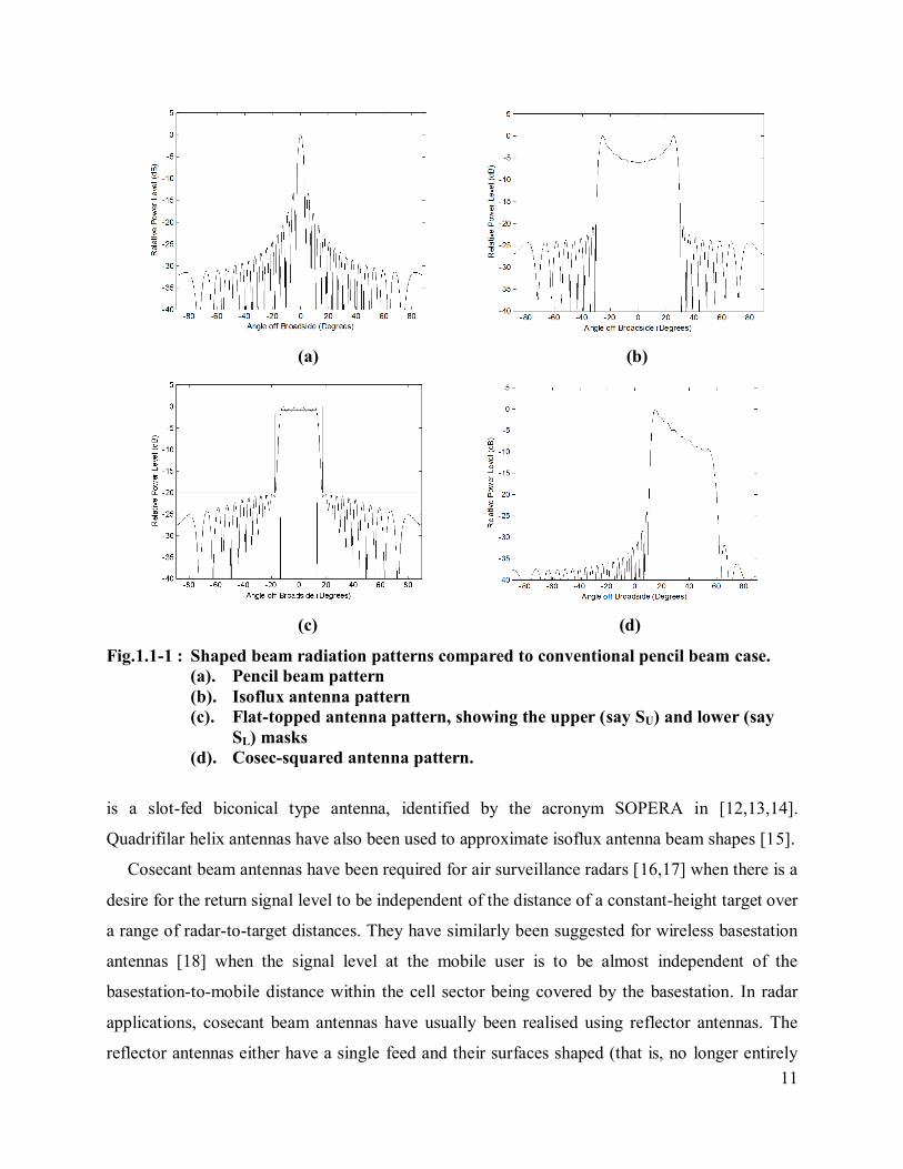
[1,2,3]. In this thesis we confine attention to isoflux beams, cosecant beams, and sectoral beams
(also called flat-topped beams). These are qualitatively illustrated in Fig.1.1-1 along with that of
the usual pencil beam. Each of these pattern shapes is considered in turn in later sections of the
thesis, and further quantitative detail will be given then (including derivations of their ideal
pattern shapes), along with further comments on the applications for which such shaped beams
are desirable. Full control of the shape of an antenna's radiation pattern can only be achieved if
the amplitude and the phase of the antenna's aperture distribution can be independently
controlled.
Earth-coverage or isoflux antennas (which are mounted on satellite payloads) are those that
have a broad pattern that is shaped in a way that results in equal field strength at all points on the
Earth within some defined field of view (FOV) of the satellite [4]. A variety of antenna types
have been employed in efforts to obtain antennas with isoflux radiation patterns for both
geostationary earth orbit (GEO) and low earth orbit (LEO) satellites. Horn antennas with rings at
the aperture are described in [5-10]. As the satellite orbital height decreases it is increasingly
difficult to obtain the desired wide beam width using such horn antennas; it is also difficult to
excite an increasing number of outer rings. For example, the Globalstar satellites which had H =
1400 km and hence an edge of coverage (EOC) angle of 52.4 used horns for telemetry, tracking
and command (TT&C) antennas, but achieved only "near isoflux type pattern performance" from
nadir to 40 off of nadir" [9]. Other authors who have used ringed horns also considered cases
for which the EOC was between 40 and 45 [6,7,8]. EOC angles larger than this require
alternative antenna configurations. One antenna geometry that can achieve EOC angles as large
as 65 consists of a shaped reflector with a rear-radiating feed [11]. They have excellent
performance out to wide EOC angles, but near boresight they depart from the ideal isoflux
pattern. A third configuration that has been used in an attempt to satisfy wide EOC requirements
11
(a) (b)
(c) (d)
Fig.1.1-1 : Shaped beam radiation patterns compared to conventional pencil beam case.
(a). Pencil beam pattern
(b). Isoflux antenna pattern
(c). Flat-topped antenna pattern, showing the upper (say SU) and lower (say
SL) masks
(d). Cosec-squared antenna pattern.
is a slot-fed biconical type antenna, identified by the acronym SOPERA in [12,13,14].
Quadrifilar helix antennas have also been used to approximate isoflux antenna beam shapes [15].
Cosecant beam antennas have been required for air surveillance radars [16,17] when there is a
desire for the return signal level to be independent of the distance of a constant-height target over
a range of radar-to-target distances. They have similarly been suggested for wireless basestation
antennas [18] when the signal level at the mobile user is to be almost independent of the
basestation-to-mobile distance within the cell sector being covered by the basestation. In radar
applications, cosecant beam antennas have usually been realised using reflector antennas. The
reflector antennas either have a single feed and their surfaces shaped (that is, no longer entirely
12
parabolic) to obtain the cosecant beam [19,20], or are parabolic but have several feeds (eg.
twelve horns in the case of the German ASR-910 air surveillance radar) that allow the beam to
be shaped in the vertical plane [21]. In wireless networks, arrays [22] are more common. Note
that the usual situation for radar applications is that cosecant beams are wanted in the vertical
plane and the usual pencil beam pattern in azimuth. In wireless networks, the cosecant pattern is
also needed in the vertical plane but sectoral beams (discussed in the next paragraph) are
normally required in the horizontal plane.
Flat-topped (or sectoral) beam patterns have been used in satellite communications systems
and microcell wireless networks. This capability has been achieved using shaped and/or multi-
feed reflectors [23] and conventional dielectric lenses [24,25,26], or arrays [27] with intricate
beamforming networks.
1.2 PRINTED LENS / TRANSMITARRAY ANTENNAS
Whereas the various realizations of shaped beam antennas may have good resulting radiation
pattern performance, they are all somewhat complex. In publications [28-30] printed free-
standing phase shifting surfaces (PSSs) were devised, and their effectiveness in realizing
transmitarray antennas with pencil beam radiation patterns, applications in which only phase
correction over the aperture is required for very acceptable performance, was demonstrated. Such
devices are in essence all-pass networks, because they are intended to maximize the transmission
amplitude at all points over the aperture but implement phase control there. In order to allow for
beam shaping, the PSS concept was extended [31] to include independent control of both the
amplitude and phase, and referred to as a phase and amplitude shifting surface (PASS). It was
applied to the realization of a transmitarray with a flat-topped beam. A significant advantage of
this proposed method is that the beam shaping can be achieved easily with a simple technique
that results in a relatively low-cost1, light, thin and flat surface suitable for mass production. It is
in principle no more difficult to design for shaped beams than pencil beams, and the resulting
structure need be no more complicated either. However, while [31] demonstrated the proof of
concept, the measured radiation patterns of the fabricated PASS transmitarray antenna showed
lower directivity levels, much higher sidelobe levels, and a larger in-beam ripple, than was
expected. The reasons were identified in [31] but, before we can discuss these, and how this
1 Compared to the other shaped beam antenna configurations mentioned in Section 1.1.
13
thesis aims to contribute to an improved aperture distribution synthesis process that might
circumvent some of these issues, the technical basics of the PSS printed lens / transmitarray
antenna need to first be described.
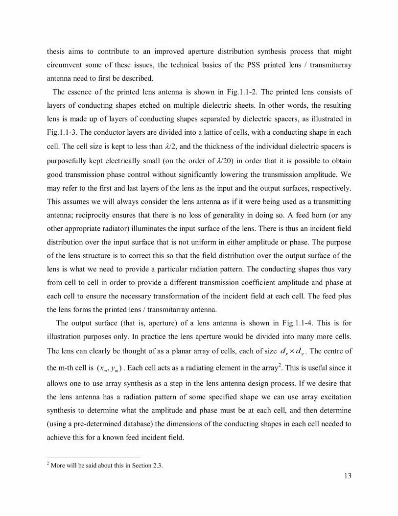
The essence of the printed lens antenna is shown in Fig.1.1-2. The printed lens consists of
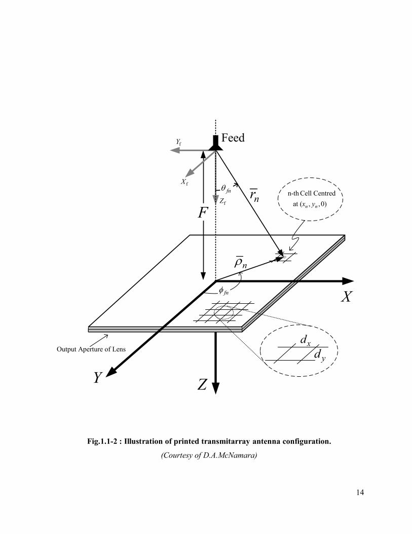
layers of conducting shapes etched on multiple dielectric sheets. In other words, the resulting
lens is made up of layers of conducting shapes separated by dielectric spacers, as illustrated in
Fig.1.1-3. The conductor layers are divided into a lattice of cells, with a conducting shape in each
cell. The cell size is kept to less than /2, and the thickness of the individual dielectric spacers is
purposefully kept electrically small (on the order of/20) in order that it is possible to obtain
good transmission phase control without significantly lowering the transmission amplitude. We
may refer to the first and last layers of the lens as the input and the output surfaces, respectively.
This assumes we will always consider the lens antenna as if it were being used as a transmitting
antenna; reciprocity ensures that there is no loss of generality in doing so. A feed horn (or any
other appropriate radiator) illuminates the input surface of the lens. There is thus an incident field
distribution over the input surface that is not uniform in either amplitude or phase. The purpose
of the lens structure is to correct this so that the field distribution over the output surface of the
lens is what we need to provide a particular radiation pattern. The conducting shapes thus vary
from cell to cell in order to provide a different transmission coefficient amplitude and phase at
each cell to ensure the necessary transformation of the incident field at each cell. The feed plus
the lens forms the printed lens / transmitarray antenna.
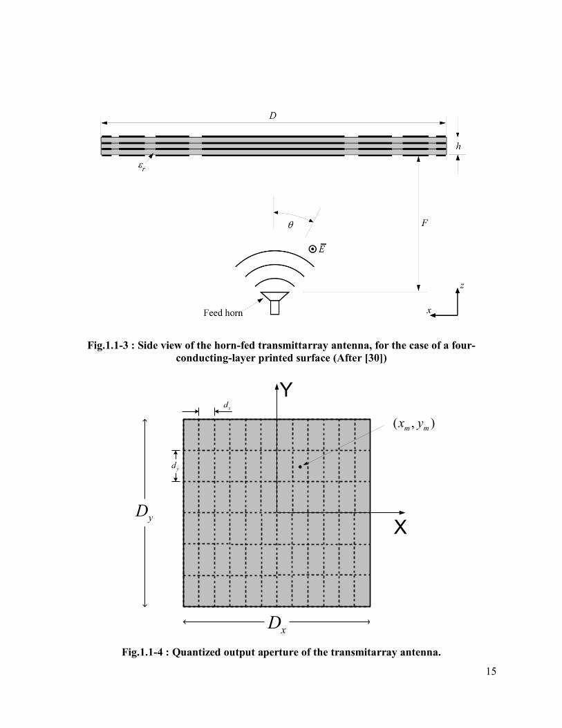
The output surface (that is, aperture) of a lens antenna is shown in Fig.1.1-4. This is for
illustration purposes only. In practice the lens aperture would be divided into many more cells.
The lens can clearly be thought of as a planar array of cells, each of size x yd d . The centre of
the m-th cell is ( , )m mx y . Each cell acts as a radiating element in the array2. This is useful since it
allows one to use array synthesis as a step in the lens antenna design process. If we desire that
the lens antenna has a radiation pattern of some specified shape we can use array excitation
synthesis to determine what the amplitude and phase must be at each cell, and then determine
(using a pre-determined database) the dimensions of the conducting shapes in each cell needed to
achieve this for a known feed incident field.
2 More will be said about this in Section 2.3.
14
X
Y Z
nr
n
Feed
F
xd
yd
n-th Cell Centred
at ( , ,0)n nx y
fY
fZ
fX
fn
fn
Output Aperture of Lens
Fig.1.1-2 : Illustration of printed transmitarray antenna configuration.
(Courtesy of D.A.McNamara)
15
Fig.1.1-3 : Side view of the horn-fed transmittarray antenna, for the case of a four-
conducting-layer printed surface (After [30])
Y
X
( , )m mx y
xd
yD
xD
yd
Fig.1.1-4 : Quantized output aperture of the transmitarray antenna.
16
We are now able to continue the discussion of the reasons, identified in [31], for the measured
radiation pattern performance of the flat-topped beam lens in the latter reference not as being
quite what was expected. When the database used in the design of the PASS transmitarray
structure was set up the conducting element was considered to be resident in an infinite periodic
array of identically-sized elements, and the amplitude and phase of the structure's plane wave
transmission coefficient computed. This was repeated for different element dimensions and the
database of transmission coefficients versus these dimensions is tabulated. The correct element
size was then selected for each cell in the PASS structure to obtain the desired amplitude and
phase at each point over the output aperture of the structure. In the final PASS lens the elements
in adjacent cells are of course not identical; if this were not so it would defeat the whole purpose
of their being used to control the aperture distribution. Thus the actual environment of each
element is not precisely the same as that experienced by the element in the infinite periodic
environment (of identical elements) used in establishing the above-mentioned database. In most
cells, the database transmission coefficient values are sufficiently accurate since there are only
small changes in the conductor shape on adjacent cells, ensured by selecting a sufficiently small
cell size. The exception occurs in the vicinity of aperture phase transition boundaries, where
there are large "discontinuities" in the shape of adjacent elements. The pattern degradation due to
such discontinuities has been noted in [31] in the context of reflectarray antennas (which is
concerned with reflection rather than transmission coefficients), and is suspected [31] to be the
first reason for the pattern degradation observed in the case of the flat-topped PASS lens antenna
as well. A second reason for the less-than-favourable radiation patterns of the flat-topped PASS
antenna is the fact that, in setting up the database for [31], it was always assumed that the
incident plane wave had normal incidence. Thus the differing incidence angles of the feed fields
at different points on the input side of the actual printed lens were not taken into account.
Although not specifically mentioned in [31] a third reason that, like the second, is inherent to the
PASS structure, might be the fact that the structure requires the amplitude of the reflection
coefficient to become large whenever the excitation amplitude (controlled using the transmission
coefficient amplitude) at some cells on the output surface of the aperture is to be reduced. This
implies backscattering from the particular cell(s) back to the feed, which is analogous to

17
spillover loss in reflector and reflectarray antennas, and so will lead to decreased gain3. This is
less severe with PSS structures (which are used for pencil beams), in which maximum
transmission amplitude is always desired and only the transmission phase is varied. Finally, a
fourth reason might also be the fact that the database has a finite number of complex
transmission coefficient (Tn) values to choose from. In [31] a synthesis process was used to find
the continuous aperture distribution needed to give the flat-topped beam. This continuous
distribution was then sampled to find the required Tn for each cell. These values are not all
available in the database, and the “nearest” database value4 is used instead.
1.3 THE CONSTRAINED ARRAY ELEMENT EXCITATION SYNTHESIS
PROBLEM
The array antenna excitation synthesis problem consists of finding the complex excitations
(that is, the excitation amplitudes and phases) of the elements of a given array to achieve a
specific radiation pattern performance. A more detailed review of excitation synthesis methods is
provided in Chapter 2. Suffice it to state here that whereas the problem of excitation synthesis
has been a subject of study since the 1940s, classical methods based on the use of polynomials
do not allow the imposition of restrictions on the values that the excitation amplitudes and phases
of the elements may take, or the synthesis of excitation sets that provide radiation patterns of
some desired arbitrary shape. These classical methods also adjust only the amplitudes of the
excitations, the phases being assumed to be the same for all elements, and the excitation
amplitudes5 may take on any value in the range zero to unity. In other words there are no
constraints on the excitation amplitudes. The more serious limitation as regards the goals of this
thesis is the fact that such classical methods are generally used for pencil beams and difference
beams. Nevertheless, such methods now serve as benchmarks against which to measure
computationally based techniques.
More general numerical approaches, on the other hand, allow one to set more complex pattern
shape specifications and permit one to place constraints on the excitations. These numerical
3 It can also degrade the input reflection coefficient of the feed. 4 More will be said about this in Chapter 3. 5 We will always work with the normalized excitation amplitudes, for which the largest value is always 1.0, and the
smallest value may be anything in the range 0.0 to 1.0.
18
optimisation based methods6 (which exploit genetic algorithms, particle swarm optimisation,
simulated annealing, gradient methods, or some other numerical optimisation algorithm) require
users to select an objective function whose minimisation they believe will lead to the best
solution of the problem they have in mind. Both pattern and excitation constraints have to be
incorporated into a single objective function whose variables are the complex excitations of the
array. The objective function must favour radiation patterns close to the desired ideal one, and
penalize excitations that fall outside the allowed complex values. Good results can only be
achieved with the proper experience. The process of selecting this objective function is thus
unavoidably somewhat “subjective”, and different solutions are obtained if the objective
functions are altered. The reason is of course that, while a simulated annealing algorithm (for
instance) might provide a global optimum of the objective function used, the said objective
function may not fully represent the array synthesis goals and constraints. Thus a global
optimum of the synthesis problem may not be reached even though a global optimum of the
specified objective function may be reached. This aspect of numerical optimisation based
excitation synthesis methods can be removed for certain classes of array excitation synthesis that
can be formulated as so-called convex programming problems7, which are more general than
those that can be approached by classical methods, but not sufficiently general for the type of
synthesis we wish to perform in this thesis.
An alternative numerical approach is that of the method of generalised projections8. This
obviates the need to define such overall objective functions. The array synthesis problem is
instead viewed as determining the intersection of two sets. The first is the set of all radiation
patterns possible with the given array geometry when the excitations comply with the required
excitation constraints. The second is the set of all radiation patterns possible with the given array
that comply with the required radiation pattern constraints. The method can be described as
synthesis in “radiation pattern space”. The same projection method can also be used in the
“excitation space”. The synthesis problem in the latter case is one of finding the intersection of
the set of all excitations that satisfy the specified excitation constraints, and the set of all
excitations that produce radiation patterns that satisfy the specified pattern constraints. Array
synthesis procedures that use some form of the method of projections are particularly attractive
6 Discussed in Section 2.5. 7 Mentioned in Section 2.6. 8 Reviewed in Section 2.7.
19
because of the quite natural way that a wide variety of desirable constraints (eg. excitation
constraints) can be implemented with a reliability not possible using other approaches. We will
use the method of projections in the work of this thesis.
1.4 OVERVIEW OF THE THESIS
The goal of this thesis is the development of synthesis methods that could be used in the
design of printed lenses to achieve shaped patterns, but subject to various constraints on the
transmission coefficients of the lens elements. The hope is that by using aperture control it might
be possible to overcome the problem issues identified in Section 1.1 and yet achieve reasonably
good shaped beam pattern performance.
Chapter 2 provides a review of array pattern synthesis methods, with an emphasis on those
methods relevant to the aims of this thesis. The method of projections is identified there as being
that most applicable for present purposes. A tutorial-like elucidation of the method of projections
in an applications-oriented format is provided. We give a systematic description of three classes
of shaped beam, namely flat-topped beams, isoflux beams and cosecant beams, which are used in
practice. Quantative means of specifying the shaped beams are given. We define what we mean
by radiation pattern masks.
In Chapter 3 we develop both serial and parallel projection methods (for the synthesis of
shaped beams) that operate in lens element transmission coefficient space9. Thus the
transmission coefficients of the printed lens elements (or cells) are directly the variables in the
synthesis process. This makes it possible to immediately perceive what influence constraints on
the actual transmission coefficients have on the possible radiation pattern performance. In
addition, we develop an approach that allows us to constrain the transmission coefficient to
values that must be selected from a set of available transmission coefficients. We believe this
approach, as straightforward as it appears with hindsight, offers a multitude of possibilities for
printed lens antennas / transmitarrays. Transmission coefficient constraints of any kind can easily
be imposed. In the last part of Chapter 3 we describe a useful approach for conveniently
determining the starting points for a shaped beam synthesis via the projection method. Good
starting values are crucial for the success of any numerically-based synthesis method.
9 This terminology is made clear in Section 2.7.
20
Chapter 4 presents a demonstration of what is physically possible as regards the performance
of a cylindrical lens antenna for three different types of widely-used shaped beams (sector beam,
cosecant beam, and isoflux beam), when either the transmission coefficient amplitudes, or
transmission phases, or both, are restricted in some way. It appears that this is the first time that
shaped beam synthesis subject to the variety of transmission coefficient constraints has been
reported, and certainly so for the phase-only synthesis of such shaped beams or synthesis that
restricts the transmission coefficients to be members of a specified database (as an integral part
of the synthesis procedure).
1.5 REFERENCES FOR CHAPTER 1
[1] C. A. Balanis (Edit.), Modern Antenna Handbook (Wiley, 2008).
[2] J. Volakis (Edit.), Modern Antenna Handbook (McGraw-Hill, 2007)
[3] G. Thiele and W. Stutzman, Antenna Theory & Design (Wiley, 1998) Chap.8
[4] L. J. Ricardi, “Satellite Antennas”, Chapter 36 in : R.C. Johnson, Antenna Engineering
Handbook (McGraw-Hill, 1993) 3rd
Edition.
[5] D. G. Bateman, S. G. Hay, T. S. Bird & F. R. Cooray, “Simple Ka-band Earth-coverage antennas for LEO satellites", Proc. Australian Symposium on Antennas, Feb. 1999.
[6] S. G. Hay, D. G. Bateman, T. S. Bird and F. R. Cooray, “Simple Ka-band earth-coverage
antennas for LEO satellites,” in IEEE Antennas and Propagation Soc. Symp., vol.1, pp. 708-711,1999.
[7] P. Brachat, “Sectoral patern synthesis with primary feeds”, IEEE Trans. Antennas
Propagat., vol.42, no. 4, pp. 484-491, April 1994.
[8] P. Metzen, “Satellite communications antennas for Globalstar“, Proc. Int. Antennas Symp.
(JINA), Nice, France, pp.574-583, Nov.1996.
[9] F .J. Dietrich, P. Metzen & P. Monte, “The Globalstar cellular satellite system”, IEEE Trans. Antennas Propagat., vol.46, no. 6, pp. 935-942, June 1998.
21
[10] L. T. Hildebrand, D. A. McNamara & G. Arbery, “Low-cost physically-small TT&C
antennas for LEO satellite applications”, Proc. 11th CASI Conference on Astronautics
(ASTRO’2000), Ottawa, Canada, 7-9 November 2000.
[11] A. Kumar, “Highly shaped beam telemetry antenna for the ERS-1 satellite”, IEE Proc., Vol.134, Pt.H, No.1, pp.106-108, Feb.1987.
[12] J. E. Fernández Del Rio, A. Nubla, L. Bustamante & K. van’t Klooster, “SOPERA: A new
antenna concept for low earth orbit satellites,” in IEEE Antennas and Propagation Soc. Symp. Digest, Vol. 1, pp. 688-691, June 1999.
[13] J. E. Fernández Del Rio, A. Nubla, L. Bustamante, F. Vila, K. van’t Klooster and
A.Frandsen, “Novel isoflux antenna alternative for LEO satellites downlink", Proc. 29th
European Microwave Conference, pp.154-157, Munich, Germany, 1999.
[14] RYMSA, Ctra. Campo Real, Km 2, 100– 28500 Arganda del Rey, Madrid, Spain
(www.rymsa.com).
[15] G. van Dooren & R.Cahill, "Design, analysis and optimisation of quadrifilar helix antennas
on the European Metop spacecraft", Proc. Int. Conf. Antennas & Propagation, pp.1.536-
1.542, Edinburgh, United Kingdom, 1997.
[16] M. I. Skolnik, Introduction to Radar Systems (McGraw-Hill, 1962).
[17] S. Drabowitch, A. Papiernik, H. D. Griffiths, J. Encinas & B. L. Smith, Modern Antennas (Springer, 2005) 2
nd Edition.
[18] E. Holzman, “Pillbox antenna design for millimeterwave base-station applications”, IEEE
Antennas & Propagation Magazine, Vol.45, No.1, pp.27-37, Feb.2003.
[19] M. I. Skolnik (Edit.), Radar Handbook (McGraw-Hill, 1990) 2nd
Edition.
[20] M. M. S. Taheri, A. R. Mallahzadeh & A. Foudazi, “Shaped beam synthesis for shaped
reflector antenna using PSO algorithm”, Proc. 6th European Conf. Antennas Propagat.
(EuCAP), Prague, Czech Republic, March 2012.
[21] L. I. Vaskelainen & K. J. Markus, “Array-fed parabolic-cylindrical reflector antenna for multifunction surveillance radar”, IEE Radar Conf., (Radar 97), pp.379-382, Oct. 1997.
[22] K. Y. Hui and K. M. Luk, “Design of wideband base station antenna arrays for CDMA 800
and GSM 900 systems”, Microwave Optical Tech. Letters, Vol.39, No.5, pp.406-409, 2003.
22
[23] S. K. Rao and M. Q. Tang, “Stepped-reflector for dual-band multiple beam satellite
communications payloads”, IEEE Trans. Antennas Propagation, 54 (2006), 801-811.
[24] R. Sauleau and B. Bares, “A complete procedure for the design and optimization of
arbitrarily-shaped integrated lens antennas”, IEEE Trans. Antennas Propagation, 54
(2006), 1122-1133.
[25] N. T. Nguyen, R. Sauleau, L. Le Coq, “Lens antennas with flat-top radiation patterns:
Benchmark of beam shaping techniques at the feed array level and lens shape level”, Proc.
3rd
European Conf. Antennas Propagat. (EuCAP), pp. 2834 – 2837, March 2009.
[26] C. A. Fernandes, “Shaped dielectric lenses for wireless millimeter-wave communications”,
IEEE Antennas Propagation Mag., 41 (1999), 141-150.
[27] S. H. Duffy, D. D. Santiago and J. S. Herd, “Design of overlapped subarrays using an
RFIC beamformer”, IEEE Int. Antennas Propagation Symp. Digest, USA, (2007) 1949-
1952.
[28] N. Gagnon, A. Petosa & D. A. McNamara, “Comparison between Conventional Lenses and
an Electrically Thin Lens Made Using a Phase Shifting Surface (PSS) at Ka Band”, in
Loughborough Antennas & Propagation Conference (LAPC 2009), Loughborough, UK, pp.
117-120, November 2009.
[29] N. Gagnon, A. Petosa & D. A. McNamara, “Thin Microwave Phase-Shifting Surface (PSS)
Lens Antenna Made of Square Elements”, Electronics Letters, vol. 46, no. 5, pp. 327-329,
March 2010.
[30] N. Gagnon, A. Petosa & D. A. McNamara, “Thin Microwave Quasi-Transparent Phase-
Shifting Surface (PSS)”, IEEE Transactions on Antennas and Propagation, vol. 58, no. 4,
pp. 1193-1201, April 2010.
[31] N. Gagnon, A. Petosa & D. A. McNamara, "Electrically Thin Free-Standing Phase and
Amplitude Shifting Surface for Beam Shaping Applications", Microwave & Optical
Technology Letters, Vol.54, No.7, pp.1566-1571, July 2012.
[32] M. A. Milon, R. Gillard and H. Legay, "Rigorous analysis of the reflectarray radiating
elements : Characterisation of the specular reflection effect and the mutual coupling effect",
29th
ESA Antenna Workshop, Netherlands, 2007.
23
CHAPTER 2
Review of Array Antenna Excitation Synthesis Techniques
2.1 INTRODUCTION
Searches of the technical literature on array excitation synthesis reveal an enormous number
of papers on the topic, starting in the 1940’s and continuing unabated up to the present time. A
few of the early papers on polynomial-based synthesis methods continue to be of importance as
benchmarks against which to rate numerical synthesis techniques used to obtain pencil beams.
However, numerical techniques are able to synthesize radiation patterns of a more general
nature. Such methods also allow one to build in excitation constraints, something that the
polynomial-based approaches are not able to do. Many numerical synthesis methods have been
developed, and a review of all work on the subject would be a tome in itself. Fortunately certain
of these techniques have proved to be superior, or have been subsumed into more general
versions of some method. In order to make this review both manageable and relevant to the
present thesis, we make the following assumptions:
We are interested in linear and planar arrays10
only, with potentially unequal inter-element
spacings along the x- and y-axes over the aperture in the planar array cases. Thus conformal
arrays are not considered at all in the review.
We are interested in arrays with rectangular lattices only. Thus arrays with circular grids are
not included in the review.
We are interested in fully populated arrays. Thinned arrays are kept out of the purview of the
present research work.
We are interested in techniques for the direct synthesis of arrays of discrete elements. Thus
we will not make reference to methods that synthesize continuous aperture distributions and then
sample these in some way in order to apply to the discrete case.
10 We will in this thesis eventually concentrate on linear arrays only, as mentioned in Section 1.4. However, methods
applicable to planar arrays with rectangular lattices are also applicable to linear arrays, and hence form part of this
review, but only so far as their use in linear array work is concerned.
24
Section 2.2 will summarize the analysis used to find the radiation patterns of arrays with
specified excitations, and specifically those expressions needed for the work in this thesis. This is
needed before any synthesis can be done. Before proceeding to a review of array synthesis
methods, we will in Section 2.3 elaborate on the connection between printed lens / transmitarray
antennas and array synthesis. Classical synthesis methods are reviewed in Section 2.4. Then
Section 2.5 reviews synthesis methods based directly on numerical optimization, but only those
that have stood the test of time and have not been superseded. Such methods find widespread use
in antenna engineering. Although convex programming is a numerical optimisation procedure, it
is set apart from the rest in Section 2.6, for reasons that will be stated there.
Section 2.7 describes the principles behind another class of numerical synthesis techniques,
namely the method of generalized projections. This will be the chosen synthesis method for the
work of this thesis, for reasons that will become apparent in later sections. Quite a bit of
background on it will therefore be given in order to lay the foundations for Chapter 3. Section
2.7.2 describes the various versions of the method in general terms11
. Although, at least for
engineers such as the present author, descriptions of the method in many papers might at first
seem unconnected to reality, the subject quickly begins to make sense once concrete forms of the
various operators and sets have been defined for a particular application. Since the actual
implementation must always be done in terms of matrices, we will write operators and functions
in terms of matrices and column-vectors, respectively, right from the start of Section 2.7.3
onwards.
2.2 ARRAY PATTERN ANALYSIS EXPRESSIONS
2.2.1 General Remarks
All analysis will be at a single frequency at a time, and so we will work with phasor
quantities. We are interested in the far-zone fields only, and can thus write the electric field of
the antenna in the form
( , , ) ( , )jkre
r Er
E (2.2-1)
11 The method has been used for many types of problem in electrical engineering (eg. image restoration) and not
only array synthesis.

25
where r is the distance from the coordinate origin located in the vicinity of the array antenna, ( , )
is the usual spherical coordinate angle pair, and 0 02 /k is the free-space
wavenumber. In the previous expression is the free space wavelength, 2 f the radial
frequency, and f the frequency in Hz. As in most antenna work the distance dependent term can be
suppressed and we can work with the direction dependent term ( , )E only. Nevertheless, ( , )E
will still be referred to it as the ‘electric field’, as is customary in antenna work. It is convenient to
define the following quantities:
A single index n will be used to number the elements of the array. The total number of elements
in the array is eN , so that n = 1,2,….., eN .
The location of the n-th element in the array is ( , , )n n nx y z .
The relative complex excitation of the n-th element is
nj
n na a e
(2.2-2)
The far-zone radiation pattern of the n-th element in the array, with 1na , when located at the
origin of the coordinate system, is
( ) ( ) ( )ˆ ˆ( , ) ( , ) ( , ) n n nE E E (2.2-3)
It then follows that by superposition the electric field of the entire array is [1]
sin cos sin sin cos( )
1
( , ) ( , )e
n n n
Njk x jk y jk zn
n
n
E a E e e e
(2.2-4)
If, as in most arrays, the elements are identical, then it is almost exactly true12
that the radiation
patterns of the individual elements are also identical (except for a phase factor dependent on its
location in the array). We then can write ( ) ( , ) ( , )n eE E for all n, and (2.2-4) becomes
12 Elements near the edges of the array will in practice have radiation patterns that are slightly different from the rest even though they may be structurally identical. However, if the array is not too small, the effect of this difference
between the in situ patterns of the elements is small. Then the radiation patterns of all elements can be assumed to be
identical, except for the location-dependent phase factor in (2.2-4). This is not true in conformal arrays for which the
elements do not all point in the same direction; but as stated earlier conformal arrays are outside the scope of this
thesis.

26
sin cos sin sin cos
1
( , ) ( , ) ( , ) ( , )e
n n n
Njk x jk y jk ze e
n
n
E E a e e e E F
(2.2-5)
with
cossinsin
1
cossin),( nn
e
n zjkyjkN
n
xjk
n eeeaF
(2.2-6)
referred to as the array factor. Identical element patterns will indeed be assumed in this thesis.
2.2.2 Planar Arrays
If the array is planar then nz is the same for all n. We write this as n refz z , and then (2.2-4)
becomes
cos sin cos sin sin( ) ( )
1
( , ) ( , ) ( , ) ( , )e
ref n n
Njk z jk x jk ye e
n
n
E e E a e e E F
(2.2-7)
and the simplified form (2.2-7) has the array factor
cos sin cos sin sin
1
( , )e
ref n n
Njk z jk x jk y
n
n
F e a e e
(2.2-8)
with n refz z usually set equal to zero.
2.2.3 Linear Arrays : General Case
In the case of a linear array the expressions for the far-zone fields are the same as those for the
general array, except that n refy y and n refz z for all elements, yielding
sin sin cos sin cos( ) ( )
1
( , ) ( , ) ( , ) ( , )e
ref ref n
Njk y jk z jk xe e
n
n
E e e E a e E F
(2.2-9)
and
sin sin cos sin cos
1
( , )e
ref ref n
Njk y jk z jk x
n
n
F e e a e
(2.2-10)
Without loss of generality (as far as linear array analysis is concerned) we can set 0ref refy z ,
implying that the elements of the linear array are located on the x-axis. The array factor is then
27
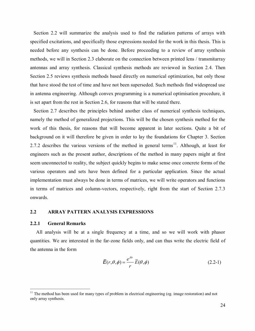
rotationally symmetric about the x-axis13
, as illustrated in Fig.2.2-1. We can therefore simply
study its shape in any one plane parallel to the x-axis, which we will choose to be the xz-plane
(for which 0 ). Thus we work with the array factor
sin
1
( )e
n
Njk x
n
n
F a e
(2.2-11)
Z
X
Y
Fig.2.2-1 : Illustration of the rotational symmetry of the array factor ( , )F of a linear
array (Adapted from [2]).
In the expressions up to this point we may number the array elements as we please. However, for
later consistency we will be specific and number them as shown in Fig.2.2-2, and then the array
factor expressions are
2sin
1
2 1sin
1
2 Elements
( )
2 1 Elements
n
n
Njk x
n
n
Njk x
n
n
a e N
F
a e N
(2.2-12)
If the elements are uniformly spaced (which will always be the case in this thesis), with inter-
element spacing d, then the x-axis location of the n-th element is
13 Although in practice the final array pattern will not be so, due to the pattern multiplication effect of the element
pattern.
28
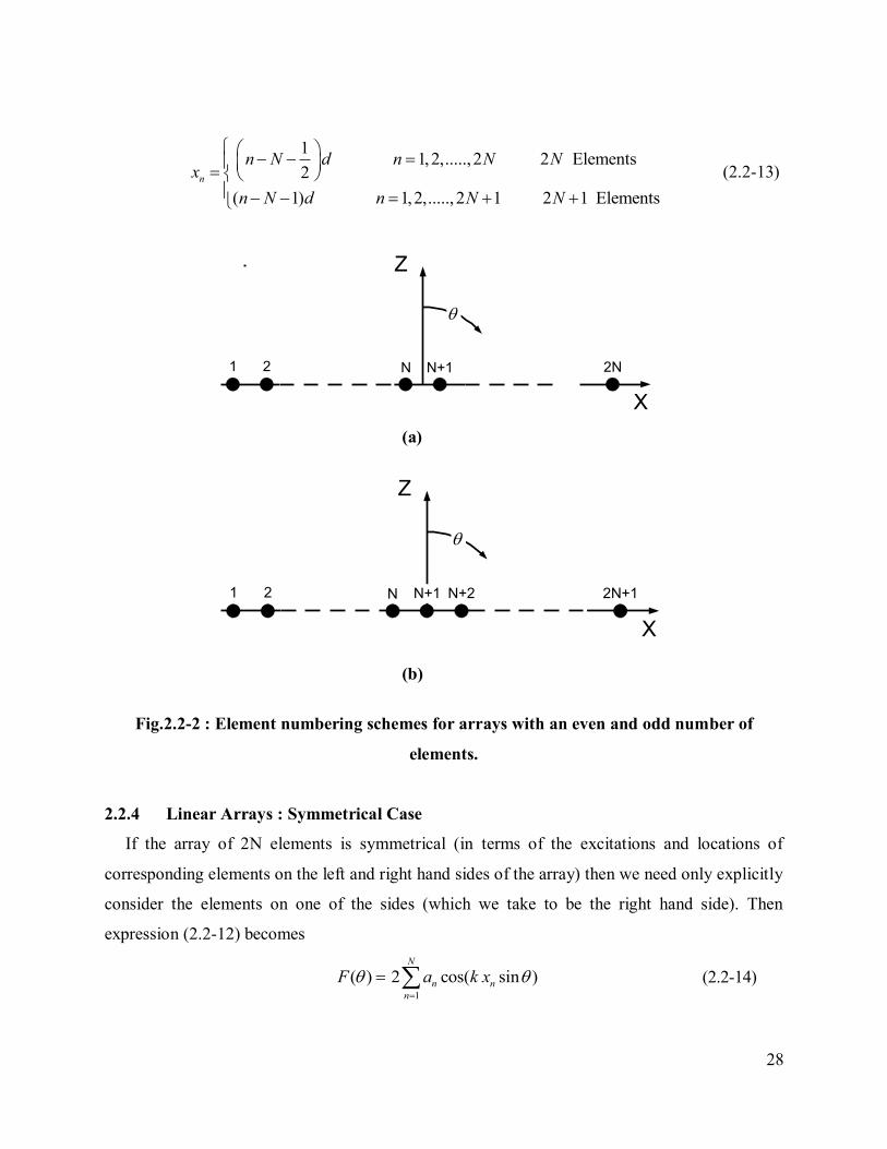
11,2,....., 2 2 Elements
2
( 1) 1,2,....., 2 1 2 1 Elements
n
n N d n N Nx
n N d n N N
(2.2-13)
Z
X
1 2 2N
N N+1
(a)
Z
X
1 2 2N+1
N N+1 N+2
(b)
Fig.2.2-2 : Element numbering schemes for arrays with an even and odd number of
elements.
2.2.4 Linear Arrays : Symmetrical Case
If the array of 2N elements is symmetrical (in terms of the excitations and locations of
corresponding elements on the left and right hand sides of the array) then we need only explicitly
consider the elements on one of the sides (which we take to be the right hand side). Then
expression (2.2-12) becomes
1
( ) 2 cos( sin )N
n n
n
F a k x
(2.2-14)
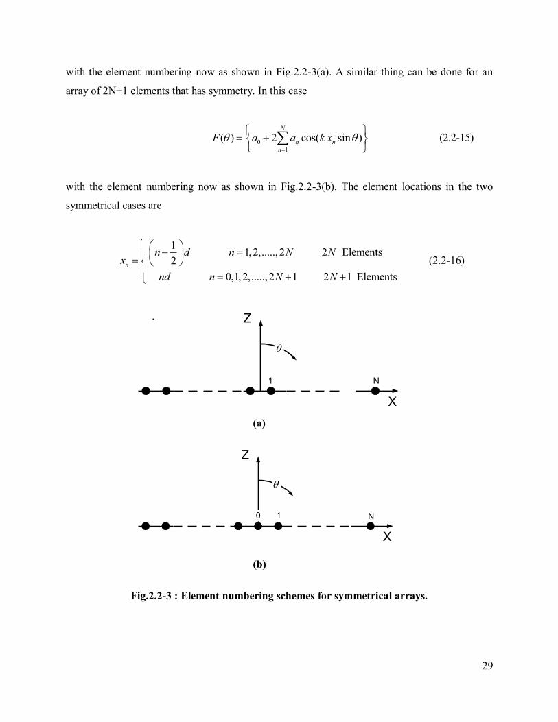
29
with the element numbering now as shown in Fig.2.2-3(a). A similar thing can be done for an
array of 2N+1 elements that has symmetry. In this case
0
1
( ) 2 cos( sin )N
n n
n
F a a k x
(2.2-15)
with the element numbering now as shown in Fig.2.2-3(b). The element locations in the two
symmetrical cases are
11,2,....., 2 2 Elements
2
0,1,2,....., 2 1 2 1 Elements
n
n d n N Nx
nd n N N
(2.2-16)
Z
X
1
N
(a)
Z
X
10
N
(b)
Fig.2.2-3 : Element numbering schemes for symmetrical arrays.

30
2.2.5 Remarks on Co- and Cross-Polarized Fields
The pattern (2.2-3) is often written in the alternative form
ˆ ˆ( , ) ( , ) ( , )co co cr crE E e E e (2.2-17)
The unit vectors indicate the orientation of the co-polarised (CO) and cross-polarised (CR) fields. In
the case of a general array we would have
( , ) ( , ) ( , )eE E F (2.2-18)
where
( , ) ( , ) ( , )e
co coE E F (2.2-19)
( , ) ( , ) ( , )e
cr crE E F (2.2-20)
and ( , )F is given by expression (2.2-6). The element pattern is
ˆ ˆ( , ) ( , ) ( , )e e e
co co cr crE E e E e (2.2-21)
In this thesis we will directly synthesise only the co-polarized fields, and so expression (2.2-19)
will be the one of interest.
2.3 PRINTED LENS / TRANSMITARRAY ANTENNA DESIGN AS AN ARRAY
EXCITATION SYNTHESIS PROBLEM
31
2.3.1 Preliminary Remarks
We intimated in Section 1.1 that the determination of the printed lens can be considered to be a
space-fed array. A more complete discussion will be given here.
2.3.2 Cylindrical Lens Antennas and Their Two-Dimensional (2D) Idealizations
The intent of this thesis is to explore means of synthesizing excitation distributions that might
provide shaped beams for printed-lens/transmitarray antennas by relying principally on the
excitation phases14
. In order to achieve this we need to develop a synthesis approach that is able
to incorporate a flexibly wide range of excitation constraints. The idea is that such excitation
constraints can be used to ensure that the resulting printed-lens/transmitarray structure (namely
distribution of elements) is such that some of the difficulties outlined in Section 1.2 are lessened.
The flexibility referred to is necessary because we do not actually want to do a phase-only
synthesis, since the inherent amplitude taper of the incident field from the feed and any
inevitable slight transmission amplitude variations that might be dictated by the particular
elements used to realize the lens, must be taken into account. We would also like the change in
the excitation from one element to another to be sufficiently small so that adjacent element
geometries are similar.
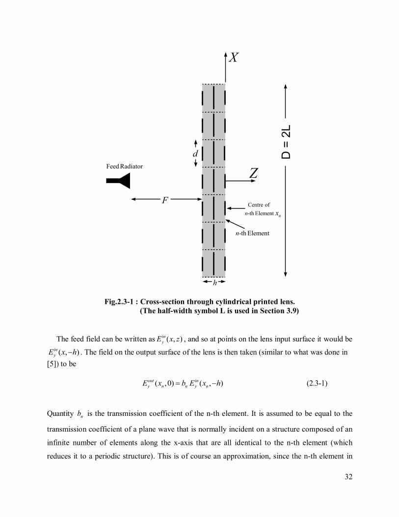
Fig.2.3-1 shows a sketch of a cylindrical lens antenna that uses three-layer strip elements, for
example. We assume that the lens is illuminated by some type of line feed15
, with a y-directed
electric field incident on the input surface of the lens. The properties of the elements are varied
along the x-axis so that a shaped beam pattern is obtained in the xz-plane (H-plane). The pattern
in the yz-plane (E-Plane) would be that of a conventional pencil beam and is largely dictated by
the pattern of the feed in that plane. This allows us to model the cylindrical lens antenna
excitation synthesis problem as a linear array synthesis one.
14 The benefits of having “phase-only” distributions to realise have already been mentioned in Section 1.3. 15 Analogous to what is used to feed cylindrical parabolic reflector, for example [3,4].
32
-th Elementn
d
Feed Radiator
F
h
Z
X
nx
Centre of
-th Elementn
D =
2L
Fig.2.3-1 : Cross-section through cylindrical printed lens.
(The half-width symbol L is used in Section 3.9)
The feed field can be written as ( , )in
yE x z , and so at points on the lens input surface it would be
( , )in
yE x h . The field on the output surface of the lens is then taken (similar to what was done in
[5]) to be
( ,0) ( , )out in
y n n y nE x b E x h (2.3-1)
Quantity nb is the transmission coefficient of the n-th element. It is assumed to be equal to the
transmission coefficient of a plane wave that is normally incident on a structure composed of an
infinite number of elements along the x-axis that are all identical to the n-th element (which
reduces it to a periodic structure). This is of course an approximation, since the n-th element in
33
the actual lens will not be surrounded by elements identical to itself. However, the success of
such an approach in reflectarray and printed lens design is overwhelmingly in favour of its
adoption. The value of nb will be a function of frequency, the properties of the substrate
material, and the widths of the conductors at each layer of the n-th cell. Tabulated values of nb
are referred to as the design database for the printed lens antenna. The above-mentioned
approximation is not the only one. In writing (2.3-1) we are implicitly assuming that ray-optic
tracking of the field is valid; that the feed field travels along a ray from the focal point to the
centre of the input surface of the n-th cell and then parallel to the z-axis through the said cell16
to
the output surface. This is not rigorously correct but has been used successfully in printed lens
design by others [5].
Each cell is viewed as an element in a linear array located along the x-axis. The excitation of the
n-th element is taken to be
( ,0) ( , )out in
n y n n y na E x b E x h (2.3-2)
The far-zone array factor in the xz-plane is then
sin
1
( )e
n
Njk x
n
n
F a e
(2.3-3)
The final far-zone pattern would include the element pattern for a single cell, which in this case
could be approximated as
sin sin2
( )
sin2
e
y
kd
Ekd
(2.3-4)
However, the cell width (equivalent to the inter-element spacing from the array viewpoint) d is
very small, and so the element pattern (2.3-4) is broad.
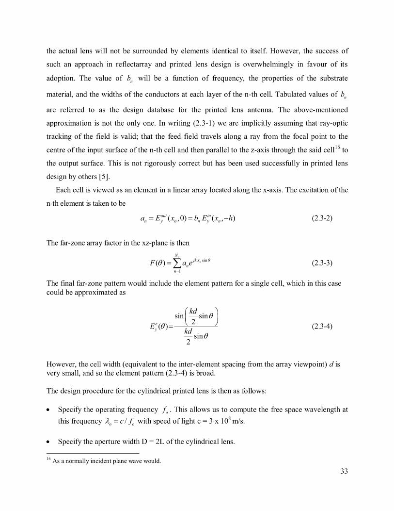
The design procedure for the cylindrical printed lens is then as follows:
Specify the operating frequency of . This allows us to compute the free space wavelength at
this frequency /o oc f with speed of light c = 3 x 10⁸
m/s.
Specify the aperture width D = 2L of the cylindrical lens.
16 As a normally incident plane wave would.
34
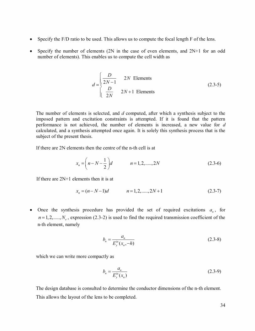
Specify the F/D ratio to be used. This allows us to compute the focal length F of the lens.
Specify the number of elements (2N in the case of even elements, and 2N+1 for an odd
number of elements). This enables us to compute the cell width as
2 Elements2 1
2 1 Elements2
DN
Nd
DN
N
(2.3-5)
The number of elements is selected, and d computed, after which a synthesis subject to the
imposed pattern and excitation constraints is attempted. If it is found that the pattern
performance is not achieved, the number of elements is increased, a new value for d
calculated, and a synthesis attempted once again. It is solely this synthesis process that is the
subject of the present thesis.
If there are 2N elements then the centre of the n-th cell is at
11,2,....., 2
2nx n N d n N
(2.3-6)
If there are 2N+1 elements then it is at
( 1) 1,2,.....,2 1nx n N d n N (2.3-7)
Once the synthesis procedure has provided the set of required excitations na , for
1,2,....., en N , expression (2.3-2) is used to find the required transmission coefficient of the
n-th element, namely
( , )
nn in
y n
ab
E x h
(2.3-8)
which we can write more compactly as
( )
nn in
y n
ab
E x (2.3-9)
The design database is consulted to determine the conductor dimensions of the n-th element.
This allows the layout of the lens to be completed.

35
2.4 CLASSICAL EXCITATION SYNTHESIS TECHNIQUES & THEIR
LIMITATIONS
2.4.1 Preliminaries
Almost all classical excitation synthesis methods are only applicable to pencil beams. Those
that can be used for the synthesis of shaped beams either do not allow any sidelobe control at all,
or allow sidelobe control but are not able to constrain the excitations in any way. All these
methods are outlined in the sub-section below. Although we will not make use of them they
allow the reader to appreciate the choice of synthesis method that will be used for the work in
this thesis.
2.4.2 Directivity Maximisation Subject to a Uniform Excitation Phase Constraint
Consider a linear array with Q elements and a fixed spacing (d) between elements. We assume
that the element excitations necessary for maximisation of the directivity in the broadside direction
are desired, without any other pattern or excitation constraints. The directivity can be written as the
ratio of two quadratic forms, both of whose operator matrices are Hermitian, with that in the
denominator being in addition positive-definite. Such properties enable the desired excitations to
be obtained directly as the solution of a set of linear simultaneous equations. Results of such
computations have been considered by Ma [6], Cheng [7], Pritchard [8], Lo et.al. [9], and Hansen
[10]. Hansen [10] has shown that for spacings above a half-wavelength, the maximum directivity is
almost identically that obtained with the elements excited with uniform amplitude and phase,
providing a pencil beam pattern. For smaller spacings the maximum directivity obtainable is
greater than that of a uniform array; this phenomenon is called superdirectivity. However, in the
latter situation there are large oscillatory variations in excitation amplitude and phase from one
element to another [10]. This is always associated with an enormously large sensitivity to small
changes in the excitations. Experimentally it is simply not easy to produce an array with a
directivity much in excess of that produced by a uniformly excited array.
2.4.3 Determination of the Array Excitations from the Array Factor Zeros
In order to appreciate the classical analytical synthesis methods to be described in the remaining
sub-sections of the present Section 2.4, it is essential to recognize that the element excitations can
be determined from the array factor zeros (in general these can be complex), and vice versa. This is
36
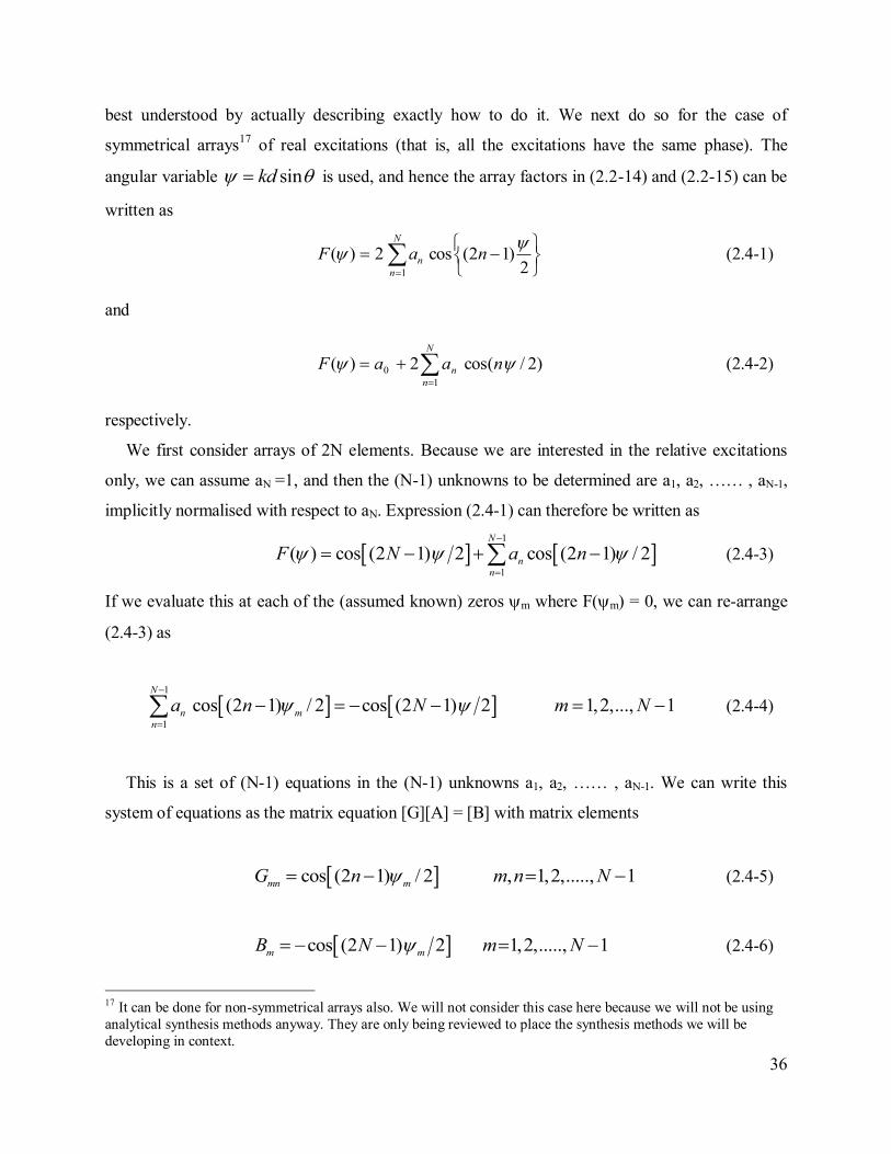
best understood by actually describing exactly how to do it. We next do so for the case of
symmetrical arrays17
of real excitations (that is, all the excitations have the same phase). The
angular variable sinkd is used, and hence the array factors in (2.2-14) and (2.2-15) can be
written as
2
)12(cos2)(1
naF
N
n
n (2.4-1)
and
)2/cos(2)(1
0 naaFN
n
n
(2.4-2)
respectively.
We first consider arrays of 2N elements. Because we are interested in the relative excitations
only, we can assume aN =1, and then the (N-1) unknowns to be determined are a1, a2, …… , aN-1,
implicitly normalised with respect to aN. Expression (2.4-1) can therefore be written as
1
1
( ) cos (2 1) 2 cos (2 1) / 2N
nn
F N a n
(2.4-3)
If we evaluate this at each of the (assumed known) zeros m where F(m) = 0, we can re-arrange
(2.4-3) as
1
1
cos (2 1) / 2 cos (2 1) 2 1,2,..., 1N
n mn
a n N m N
(2.4-4)
This is a set of (N-1) equations in the (N-1) unknowns a1, a2, …… , aN-1. We can write this
system of equations as the matrix equation [G][A] = [B] with matrix elements
cos (2 1) / 2 , 1,2,....., 1mn m
G n m n N (2.4-5)
cos (2 1) 2 1,2,....., 1m m
B N m N (2.4-6)
17 It can be done for non-symmetrical arrays also. We will not consider this case here because we will not be using
analytical synthesis methods anyway. They are only being reviewed to place the synthesis methods we will be
developing in context.
37
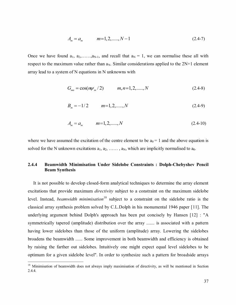
1,2,....., 1m m
A a m N (2.4-7)
Once we have found a1, a2,……,aN-1, and recall that aN = 1, we can normalise these all with
respect to the maximum value rather than aN. Similar considerations applied to the 2N+1 element
array lead to a system of N equations in N unknowns with
cos( / 2) , 1,2,.....,mn m
G n m n N (2.4-8)
1/ 2 1,2,.....,m
B m N (2.4-9)
1,2,.....,m m
A a m N (2.4-10)
where we have assumed the excitation of the centre element to be a0 = 1 and the above equation is
solved for the N unknown excitations a1, a2, …… , aN, which are implicitly normalised to a0.
2.4.4 Beamwidth Minimisation Under Sidelobe Constraints : Dolph-Chebyshev Pencil
Beam Synthesis
It is not possible to develop closed-form analytical techniques to determine the array element
excitations that provide maximum directivity subject to a constraint on the maximum sidelobe
level. Instead, beamwidth minimisation18
subject to a constraint on the sidelobe ratio is the
classical array synthesis problem solved by C.L.Dolph in his monumental 1946 paper [11]. The
underlying argument behind Dolph's approach has been put concisely by Hansen [12] : "A
symmetrically tapered (amplitude) distribution over the array ....... is associated with a pattern
having lower sidelobes than those of the uniform (amplitude) array. Lowering the sidelobes
broadens the beamwidth ...... Some improvement in both beamwidth and efficiency is obtained
by raising the farther out sidelobes. Intuitively one might expect equal level sidelobes to be
optimum for a given sidelobe level". In order to synthesize such a pattern for broadside arrays
18 Minimisation of beamwidth does not always imply maximisation of directivity, as will be mentioned in Section
2.4.4.
38
with interelement spacing greater than or equal to a half-wavelength, Dolph made use of the
Chebyshev polynomials.
Consider the problem of best approximation (in the minimax sense) of the function f(x) = 0
over19
the interval -1 x 1 by a polynomial PM(x) of specified order M. In other words, given the
above f(x), determine whatever details are needed to completely define PM(x) so that we are able to
evaluate it for any x in the above interval. Since PM(x) is a polynomial this same information will in
fact allow us to evaluate it for any - x . A purely mathematical theorem [13,14] proves that
the required polynomials are the so-called Chebyshev polynomials TM(x), defined by
1coshcosh
11coscos
1coshcosh)1(
)(1
1
1
xxM
xxM
xxM
xT
M
M (2.4-11)
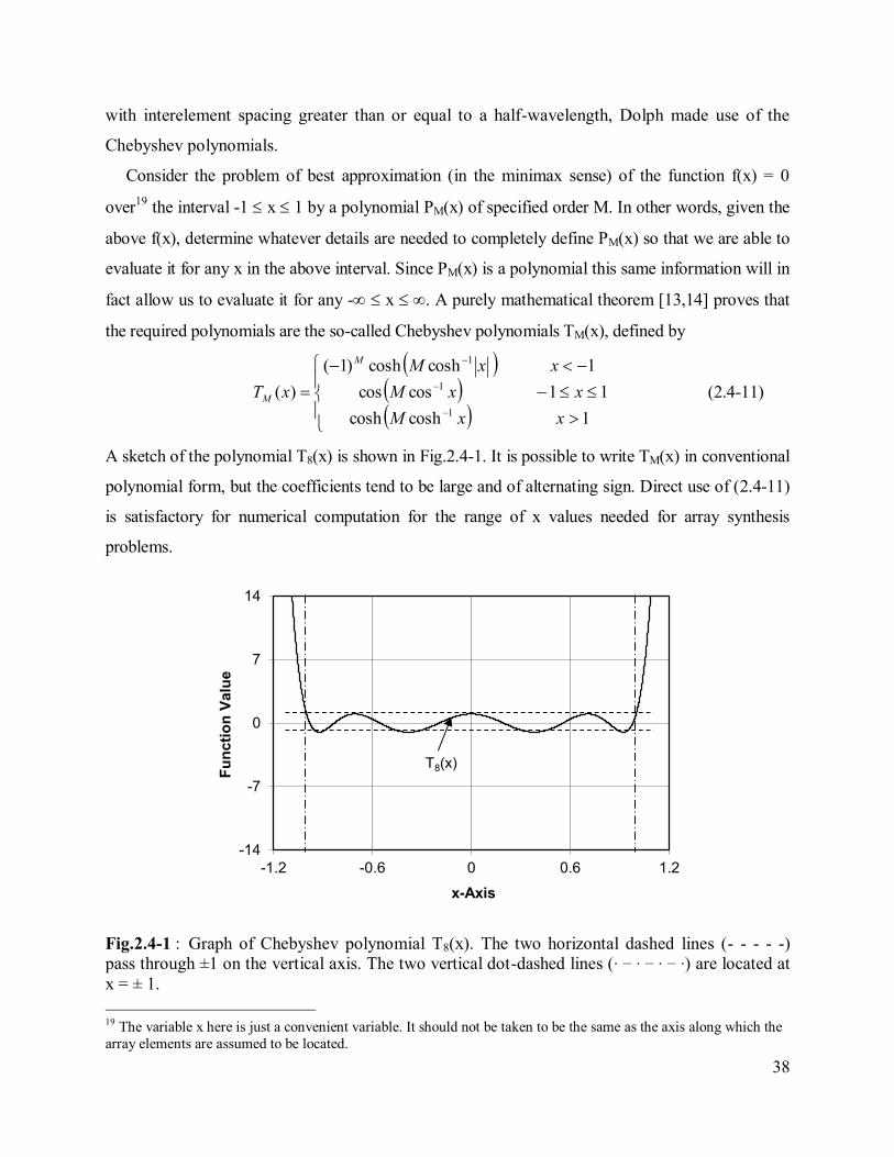
A sketch of the polynomial T8(x) is shown in Fig.2.4-1. It is possible to write TM(x) in conventional
polynomial form, but the coefficients tend to be large and of alternating sign. Direct use of (2.4-11)
is satisfactory for numerical computation for the range of x values needed for array synthesis
problems.
-14
-7
0
7
14
-1.2 -0.6 0 0.6 1.2
Fu
nc
tio
n V
alu
e
x-Axis
T8(x)
Fig.2.4-1 : Graph of Chebyshev polynomial T8(x). The two horizontal dashed lines (- - - - -)
pass through ±1 on the vertical axis. The two vertical dot-dashed lines (∙ − ∙ − ∙ − ∙) are located at
x = ± 1.
19 The variable x here is just a convenient variable. It should not be taken to be the same as the axis along which the
array elements are assumed to be located.

39
Fig.2.4-2 : Enlargement of a portion of the graph of polynomial T8(x) from Fig.2.4-1, and
quantities related to Chebyshev array synthesis.
At this point all we have are some mathematical facts. The creative idea of relating array factors
to Chebyshev polynomials, using this transformation to synthesise array excitations, and providing a
proof of the optimality of the resulting arrays, was provided by Dolph [11]. Observe from (2.4-11)
and Fig.2.4-1 that in the range 11 x the function TM(x) ripples in amplitude between the
limits 1. We next refer to Fig.2.4-2, which shows an enlarged portion of the T8(x) of Fig.2.4-1. Of
all polynomials PM(x) of degree M which pass through the given point (xo,ASLR) and which remain
within the bounds 1 in the interval x 1, the Chebyshev polynomial TM(x) minimises the length
of the interval (xo - xLR), where xLR is the largest zero of PM(x). Outside of this range of x-values
TM(x) increases hyperbolically, with TM(x)> 1. Dolph [11] recognised these properties as being
what is required to synthesise a linear array that, for a given number of elements and specified
sidelobe level, has the minimum beamwidth between first nulls. To achieve such a synthesis he used
the transformation 2cosoxx to establish a correspondence between TM(x) and an associated
array factor, with the constraint SLRM AxT )( 0 setting the required sidelobe ratio. Observe that as
varies over the visible angular range from -/2 to /2 the variable x varies from x = = xocos(kd/2)
at = - /2, to x = xo when = 0, and finally to x = at = /2. If d = /2 then = 0, while for d
> /2 we have < 0. Thus for d /2, as the observation angle varies over the visible range, the
40
range of the variable x includes all the polynomial zeros in the interval (0, xo) for either even or
odd arrays.
The polynomial T2N-1(x) is used to synthesise arrays of size 2N, and T2N(x) for arrays of size
2N+1. The zeroes of the appropriate polynomial are easily determined, from which the array factor
zeros m are calculated using the inverse of the transformation 2cosoxx . Once the latter are
known it is a matter of algebra to obtain the excitations. Dolph was able to prove [11] that the
array so synthesised is optimum in the sense that for the specified sidelobe ratio and element
number, the beamwidth (between first nulls) is the narrowest possible. Alternatively, for a
specified first-null beamwidth, the sidelobe level is the lowest obtainable from the given array
geometry. This means that it is impossible to find another set of excitation coefficients yielding
better performance, in both beamwidth and sidelobe ratio, for the given element number and
uniform spacing d. It represents a closed form solution to the optimisation problem of beamwidth
minimisation subject to sidelobe constraints.
Many expressions have been derived for the Cheyshev array excitations, the relative importance
of which have changed over the years as computational capabilities have improved. The most
straightforward approach is that which directly exploits the fact that F(m) = 0 for each of the array
factor zeros m, and which therefore (taking each of the m in turn) represents a set of simultaneous
linear equations with the excitations as the unknowns. This was described in Section 2.4.3, and
enables us to apply one of the many computationally efficient simultaneous linear equation
solver algorithms that are now so readily available as coded routines. Once the process has been
coded it is as good as, and possibly better than, “closed-form” expressions as far as numerical
computation is concerned.
The original formulation by Dolph [11] for synthesising linear Chebyshev arrays is applicable
to the case of an even (2N) or odd (2N+1) number of array elements when the inter-element
spacing d /2, where is the wavelength. The restriction on d, initially noted by Riblet [15], is
needed to ensure that the transformation responsible for the polynomial array factor
correspondence provides a radiation pattern that is optimal in the sense of yielding the minimum
first-null-beamwidth for the given number of elements and specified sidelobe ratio (SLR). As
cautioned in [1,6,10,16,17,18] this transformation does not guarantee optimality if d < /2.
Subsequent formulations [15,19,20] showed how the transformation must be altered to reclaim
41
optimality when d < /2, but only for arrays of 2N+1 elements. A means of synthesizing such
optimal arrays when there are 2N elements and d < /2 was more recently given in [21].
2.4.5 Villeneuve n -Distributions : Pencil Beam Synthesis
Optimum beamwidth arrays do not necessarily provide optimum directivity, especially if the
array is large [17]. To see this, one can consider a Dolph-Chebyshev array with a fixed sidelobe
ratio. Let the array size increase (increase the element number with the spacing held fixed), at
each stage keeping the sidelobe ratio constant and normalising the radiation pattern. This is
permissible because the directivity to be found at each stage is only dependent on the angular
distribution of the radiation and not on any absolute levels. It is then observed that the
denominator of the directivity expression is dominated by the power in the sidelobes after a
certain array size is reached, and remains roughly constant thereafter. Thus it is found that the
Dolph-Chebyshev distribution has a directivity limit [22] because of its constant sidelobe level
property, and for a given array size and maximum sidelobe level, may not be optimum from a
directivity point of view.
The above “directivity compression” is usually accompanied by an undesirable upswing in the
amplitude of the excitations near the array edges ("edge brightening"). For a given number of
elements there will be a certain sidelobe ratio for which the distribution of excitations is "just"
monotonic. If the number of elements is increased but this same sidelobe ratio is desired, the
required distribution will be non-monotonic. Increasing the sidelobe ratio (lower sidelobes) will
allow a monotonic distribution once more. Peaks in the distribution at the array ends are not only
disadvantageous in that they are difficult to implement and make an array which is realised more
susceptible to edge effects, but they are also indicative of an increase in the tolerance sensitivity
[23]. To remove these practical drawbacks a taper must be incorporated into the far-out
sidelobes. This is achieved by the Villeneuve distribution [24].
The Villeneuve distribution utilises the principle of synthesising excitation distributions by
correct positioning of the array factor zeros. The application of the approach consists of the
following steps once the number of array elements, inter-element spacing and maximum sidelobe
level have been specified :
42
Step#1 – Determine the array factor zeros for a Dolph-Chebyshev distribution on an array of the
same number of elements with the same sidelobe level, as described in Section 2.4.4. (Such an
array will have a uniform sidelobe envelope).
Step#2 – Determine the array factor zeros of a uniformly excited array of the same number of
elements. (Such an array will have a tapered sidelobe envelope).
Step#3 – Alter the zeros of the Dolph-Chebyshev array so that all except the first n -1 zeros now
coincide with those of the uniformly excited array. In addition multiply each of the first n -1
Chebyshev zeros by a dilation factor . The quantity n is referred to as the transition index. The
dilation factor is given by [24]
1
0
n
1(2N 1)cos cos (2n-1)
4Nu
(2.4-12)
where
2
0
1cosh ln 1
2Nu
(2.4-13)
and / 2010 SLR (2.4-14)
for an array of 2N+1 elements. Similar expressions are provided in [24] for an array of 2N
elements. The sidelobe ratio (in dB) is denoted by SLR.
Step#4 – Use these final zeros of the perturbed Chebyshev array to determine the final element
excitations20
.
The result will be an array factor whose near-in sidelobes are close to the maximum sidelobe
level specified, with the further out ones decreasing in level at a rate close to that of the uniformly
excited array. This behaviour has been shown to provide arrays with the desired maximum
sidelobe level but higher aperture efficiency than one would get if some arbitrary tapered excitation
distribution were to be used.
The Villeneuve distribution was generalized in [25]. Although the quantities and n are
retained, an additional parameter v , called the taper parameter is introduced. This allows the taper
rate of the sidelobe envelope to be controlled. In other words, like the Villeneuve distribution, the
Dolph-Chebyshev distribution serves as a "parent" space factor. The correct perturbation of the
zeros of this parent space factor serves to incorporate the sidelobe behaviour desired, while at the
20 In his original paper Villeneuve [24] derived closed-form series expressions for the excitations, but they are
found just as easily using the technique described in Section 2.4.3.
43
same time keeping the excitation efficiency and beamwidths as close to their optimum values as is
possible under the required sidelobe ratio and envelope taper conditions. The level of the first
sidelobe is set by the parent Dolph-Chebyshev distribution, the envelope taper rate controlled by
the taper parameter , and the point at which the required taper proper begins determined by the
transition index n . The proper choice of the values of n and for a particular application will
depend on the relative importance of the peak sidelobe level compared to that of the farther-out
sidelobes, and their effect on the excitation efficiency.
2.4.6 Analytical Shaped Beam Synthesis Methods
The array factors have the form of a Fourier series, but with the number of terms of the same
order as the number of elements in the array. An early Fourier series synthesis method does the
following : The idealized shaped pattern21
over the shaped region is expanded in a Fourier series.
The element excitations are equated to the coefficients of this Fourier series expansion. Due to
the limited number of terms in the Fourier series of the shaped pattern the resulting pattern
exhibits large ripples around the idealized shaped pattern, and high sidelobes outside the shaped
region.
An improvement on the above technique is the Woodward-Lawson [26,27] method. This
technique relies on the fact that any pattern realizable using an Ne element array can be
expressed as the weighted summation of a set of Ne orthogonal beams, each having a
“sin(Nex)/sin(x)” shape. The maximum value of each of these beams coincides with the zero in
all other beams. The synthesis technique samples the idealized shaped pattern at increments of
Ne/2. The synthesized array is thus the superposition of array factors from Ne uniform
amplitude, linear progressive phase excitations with the phase increment of each excitation such
that the array factor peak is placed at a sampling point on the idealized shaped beam. Although
the resultant array factor is equal to the idealized shaped pattern at the sample points, it also
exhibits large ripples in the shaped beam region and high uncontrollable sidelobes in the sidelobe
region.
A criticism of the Woodward-Lawson method is that it only uses data from Ne idealized
pattern sampling points, whereas there are 2Ne-2 degrees of freedom (namely Ne-1 relative
21 Please see Section 2.9 for a discussion of the idealized forms of the flat-topped, isoflux and cosecant shaped
patterns.
44
amplitudes and Ne-1 relative phases. Milne described a method [28] that effectively takes 2Ne-1
sample points, spaced at intervals 2/(2Ne-1). In essence it starts with some pencil beam pattern,
copies of which are “scanned” to have their maxima at points in the shaped region and sidelobe
region. This allows some limited control of the shaped beam region ripple and sidelobe levels.
2.4.7 Numerical Variation of the Complex Polynomial Roots
The best approach not based on numerical optimization of some objective function, or the
method of projections, is that by Orchard et al. [29]. This is an iterative method in which the
zeroes of the array factor are made complex, and their real and imaginary parts are
simultaneously adjusted in an iterative fashion so that the amplitude of each ripple in the shaped
beam region and the height of each sidelobe outside of this region are individually controlled. A
recipe for such adjustments is provided in [29], but its use of far from routine.
2.4.8 Limitation of Classical Synthesis Methods
The reader will have noticed that the methods in Sections 2.4.2 through 2.4.5 can be used for
pencil beam synthesis only. Although that in Sections 2.4.6 and 2.4.7 can be used for shaped
beam synthesis, they cannot entertain any excitation constraints. Indeed, this is not possible with
any classical analytical synthesis methods. This means that, for example, phase-only excitation
synthesis is not possible either. In classical excitation synthesis methods we have to let the
excitation amplitudes and phases “do what they please”. These methods are thus not suited to the
goals of this thesis.
45
2.5 SYNTHESIS METHODS DIRECTLY BASED ON CONVENTIONAL
NUMERICAL OPTIMISATION ALGORITHMS
2.5.1 Introduction
Excitation synthesis techniques that rely explicitly on the use of numerical optimization
algorithms all require that the synthesis requirements (both pattern and excitation constraints) be
encapsulated in a single objective function
1 2, ,.........,eobj NF a a a (2.5-1)
that is, as indicated, a function of the array excitations. There are numerous numerical
optimization algorithms that can be used to efficiently locate the minimum of a given objective
function objF . In array synthesis work these are only useful if we are able to so define objF that,
when its minimum is attained, we have an array antenna whose performance is indeed what we
seek. In other words, what we are able to achieve depends on how well we have translated our
desired antenna specifications into a mathematical expression which, when optimized, provides a
performance that meets our requirements. These requirements will be both pattern constraints
and excitation constraints.
The objective functions are non-linear, and usually have many local minima that can trap the
algorithm. Evolutionary algorithms (eg. genetic algorithm) have been successfully used to avoid
the problem of getting stuck in local minima. These global optimization approaches are very
heavy on computation, but this is less of an issue these days. One disadvantage (compared to the
projection synthesis methods to be described in Section 2.7, and which will be the chosen
method for this thesis) is that the pattern and excitation constraints are intertwined in some
objective function. It would be preferable if the excitation constraints could be made more
explicit, making it possible to more easily recognize trade-offs and to judge the plausibility of
some excitation constraint. Nevertheless such synthesis techniques, especially using the genetic
algorithm (in its many forms) as the numerical optimization algorithm of choice, could be used
for the problem of interest in this thesis. However, we have selected the projection method
described in Section 2.7, for reasons that will become clear in that section.
46
2.5.2 Least Squares Based Methods
In order to describe the least squares approach we will use the radiation pattern analysis
model in expression (2.2-19) namely22
1
( ) ( )eN
CO n n
n
E a F
(2.5-2)
where
sin( , ) njkx
nF e (2.5-3)
We will next define certain matrices that will be used in the writing of the projection synthesis
formulations in concrete terms in Section 2.7; they are provided here already because they turn
out to be equally useful for an explanation of the least-squares methods with which we are
immediately concerned in the present section. Expression (2.5-2) can be written as
1
1( ) ....... ........e
e
nCO n N
N
a
aE F F F
a
(2.5-4)
This is a continuous function over the independent variables 0 and 0 2. If we
are to actually implement any numerically based method, at some point in the procedure we of
course need to obtain a finite-dimensional and discrete representation of the pattern vector in
order to perform numerical computations. A finite-dimensional discrete pattern vector [ ]COE can
22 We discuss it for the linear array case (which is of interest in this thesis), although everything can be done for the
planar array case too. In the linear array case we can write the array factor in terms of angle only, as shown. We
will also ignore the broad element pattern. Hence the form of expression (2.5-2).
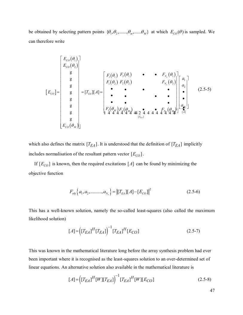
47
be obtained by selecting pattern points 1 2{ , ,......, ,...... }m M at which ( )COE is sampled. We
can therefore write
{
1
2
2 1 11 1
1
2 2 21 2
2
1 2 [ ]
[ ]
[ ][ ]
e
e
e
EA
CO
CO
N
N
CO EA
N
M M N M A
T
CO M
E
E
F FFa
F FFa
E T A
aF F F
E
g
g
g
g
g
g
g 1 4 4 4 4 4 4 44 2 4 4 4 4 4 4 4 43
g
(2.5-5)
which also defines the matrix [ ]EAT . It is understood that the definition of [ ]EAT implicitly
includes normalisation of the resultant pattern vector [ ]COE .
If [ ]COE is known, then the required excitations [ ]A can be found by minimizing the
objective function
2
1 2, ,........., [ ][ ] [ ]eobj N EA COF a a a T A E (2.5-6)
This has a well-known solution, namely the so-called least-squares (also called the maximum
likelihood solution)
1
[ ] [ ] [ ] [ ] [ ]H HEA EA EA COA T T T E
(2.5-7)
This was known in the mathematical literature long before the array synthesis problem had ever
been important where it is recognised as the least-squares solution to an over-determined set of
linear equations. An alternative solution also available in the mathematical literature is
1
[ ] [ ] [ ][ ] [ ] [ ][ ]H HEA EA EA COA T W T T W E
(2.5-8)
48
where [ ]W is a diagonal weighting vector, and superscript “H” indicates the conjugate transpose
operation. If [ ]W is selected to be the identity matrix the process reduces to conventional least
squares (also referred to as the maximum likelihood method). Relative weights must be assigned to
the weighting vector [ ]W . In array synthesis the main lobe region and each sidelobe region can be
assigned a regional weight according to their relative importance in a particular application. In other
words, the relative weights can be decreased at sampling angles that are less important as far as
precise satisfaction of the pattern constraints is concerned.
If we had [ ]COE , by which we mean its complex values, which would mean that both the
pattern amplitude and phase of the desired pattern is known at each sample angle m , then we
could simply use (2.5-7) or (2.5-8) to find [ ]A . The problem is that when we synthesize shaped
beam patterns – as will be detailed in Section 2.9 – we do not know the precise shape of the
complex pattern [ ]COE . We know only the masks within which the magnitudes of the pattern
samples ( )CO mE must lie; the phases of the complex field values ( )CO mE are not specified.
One might be tempted to declare that the pattern phase be constant with respect to . But there is
a weakness in this argument. The masks23
include not only the shaped beam region but also the
sidelobe regions. Why would the pattern phase over this entire set of pattern angles necessarily
be the same? Even within the shaped beam region the pattern phase need not be constant as a
function of . So we do not wish to impose an artificial phase on the radiation pattern (in so
doing perhaps missing some improved synthesis solution), and instead want it to develop in a
natural way according to what the physics demands. In shaped beam methods that use a least-
squares approach this is achieved by an iteration process. An initial guess (or “warm start” if we
prefer the more technical terminology) is made, and then an iterative process such as that
detailed in [30,31,32] is used to arrive at the required excitation vector [ ]A . However, the
imposition of excitation constraints is not possible using the least-squares method just described.
A least-squares method that allows phase-only synthesis (with all excitation amplitudes kept the
same) has been described [33], but it can handle only small perturbations to the phase and so is
not applicable to all beam shapes.
23 To be discussed in some detail in Section 2.9.
49
2.5.3 Use of Gradient-Based or Evolutionary Numerical Optimisation Algorithms
Once an objective function objF has been defined any numerical optimization algorithm can
be used for synthesis purposes. Gradient-based algorithms (eg. [54]) used to be utilized, but
evolutionary algorithms are now preferred. There is an enormous literature on the subject, both
in textbooks and journal papers, and the reader is referred to references [35] through [46], where
array synthesis applications are described using mainly the genetic algorithm, but also the
particle-swarm and simulated-annealing algorithms. The user has to be aware of the fact that
objective functions that not only include pattern constraints but also excitation constraints are not
as widely used in the references mentioned. Those that do include excitation constraints require
quite a bit of “tuning” before they are satisfactorily represent the synthesis goals24
. After all, we
wish to converge to an optimum of the synthesis problem. If objF is not chosen properly we might
achieve its optimum value but this might not provide us with a solution that represents the synthesis
goals. As with all numerical optimization algorithms a warm start is needed for the excitation
amplitudes and phases.
2.6 SYNTHESIS METHODS BASED ON CONVEX PROGRAMMING ALGORITHMS
Even though excitation synthesis methods based on convex programming can be classified
under the same set of methods as that in Section 2.5 – after all it is based on the minimization of
an objective function - it is often considered separately. The reason is that if it is possible to
derive an objective function that is in fact a quadratic form then the numerical optimization
algorithm known as convex programming can be used. The latter algorithm has the advantage
that it will always converge to a global optimum of the objective function. This method was used
several years ago to perform an excitation synthesis that maximizes directivity subject to
sidelobe constraints [49,50]. However, it has recently been refined in the sense that objective
functions applicable to a wider range of array synthesis problems have been derived [52 - 58].
24 This is not always apparent from the literature.
50
Nevertheless, it is still not possible to use convex programming directly if we wish to apply
excitation constraints25
. Thus the method is not germane to the problem of interest in this thesis.
2.7 EXCITATION SYNTHESIS USING THE METHOD OF GENERALIZED
PROJECTIONS
2.7.1 Introduction
In contrast to the excitation synthesis methods described in the previous three sections, the
array synthesis problem can also be viewed as determining the intersection of two sets. The first
is the set of all radiation patterns possible with the given array geometry (in other words patterns
computed using the appropriate forward operator26
for the particular geometry in question) when
the excitations comply with the required excitation constraints. The second is the set of all
radiation patterns possible with the given array that comply with the required radiation pattern
constraints. The method can be described as synthesis in “radiation pattern space”. This approach
was used in [59], with major advances to the detail and breadth of applications being made in
[60,61,62] and its use being extended to conformal arrays in [63,64,65]. These all used the so-
called generalized sequential projection method.
In [66] the same sequential projection method was used, but in the “excitation space”, the
advantage being that certain relaxation methods can be applied to speed up convergence. The
synthesis problem in the latter case is one of finding the intersection of the set of all excitations
that satisfy the specified excitation constraints, and the set of all excitations that produce
radiation patterns that satisfy the specified pattern constraints.
The generalised parallel projection method [67,68,69] was more recently introduced, albeit
not in the context of array synthesis, based on ideas originally published by Pierra [70]. This
parallel version of the method was applied in [71] to a “switched-element” pencil beam array
synthesis problem in excitation space, but has not been applied to shaped beam synthesis.
25 An exception is its use for phase-only synthesis [51], but it can handle only small perturbations to the phase, and
so is not necessarily applicable to shaped beam synthesis. 26 The forward operator will be defined in Section 2.7.4.
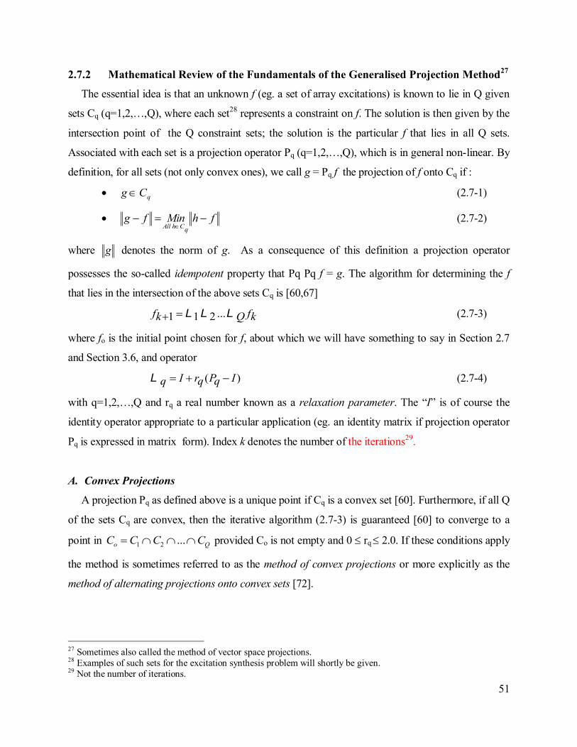
51
2.7.2 Mathematical Review of the Fundamentals of the Generalised Projection Method27
The essential idea is that an unknown f (eg. a set of array excitations) is known to lie in Q given
sets Cq (q=1,2,…,Q), where each set28
represents a constraint on f. The solution is then given by the
intersection point of the Q constraint sets; the solution is the particular f that lies in all Q sets.
Associated with each set is a projection operator Pq (q=1,2,…,Q), which is in general non-linear. By
definition, for all sets (not only convex ones), we call g = Pq f the projection of f onto Cq if :
qCg (2.7-1)
fhMinfgq
ChAll
(2.7-2)
where g denotes the norm of g. As a consequence of this definition a projection operator
possesses the so-called idempotent property that Pq Pq f = g. The algorithm for determining the f
that lies in the intersection of the above sets Cq is [60,67]
...1 1 2f fk Q k L L L (2.7-3)
where fo is the initial point chosen for f, about which we will have something to say in Section 2.7
and Section 3.6, and operator
( )I r P Iq q q L (2.7-4)
with q=1,2,…,Q and rq a real number known as a relaxation parameter. The “I” is of course the
identity operator appropriate to a particular application (eg. an identity matrix if projection operator
Pq is expressed in matrix form). Index k denotes the number of the iterations29
.
A. Convex Projections
A projection Pq as defined above is a unique point if Cq is a convex set [60]. Furthermore, if all Q
of the sets Cq are convex, then the iterative algorithm (2.7-3) is guaranteed [60] to converge to a
point in Qo CCCC ...21 provided Co is not empty and 0 rq 2.0. If these conditions apply
the method is sometimes referred to as the method of convex projections or more explicitly as the
method of alternating projections onto convex sets [72].
27 Sometimes also called the method of vector space projections. 28 Examples of such sets for the excitation synthesis problem will shortly be given. 29 Not the number of iterations.
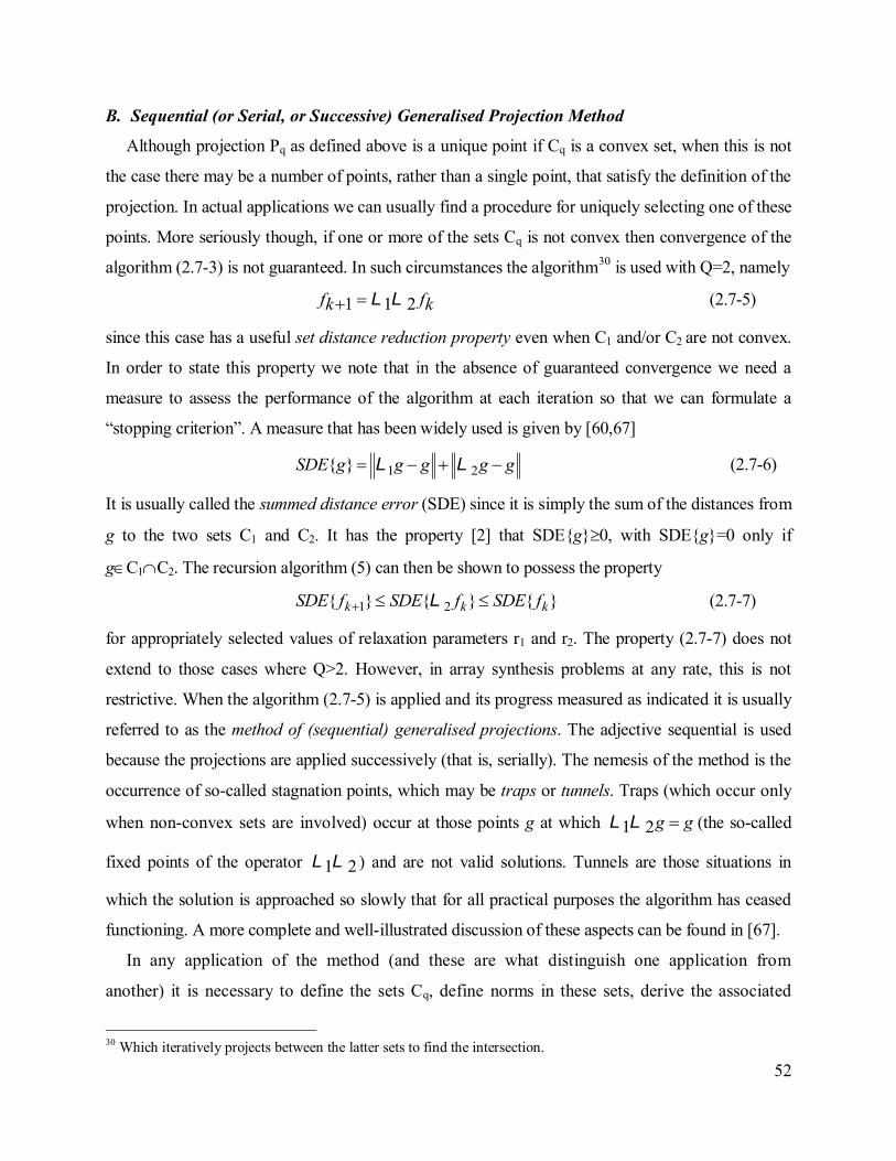
52
B. Sequential (or Serial, or Successive) Generalised Projection Method
Although projection Pq as defined above is a unique point if Cq is a convex set, when this is not
the case there may be a number of points, rather than a single point, that satisfy the definition of the
projection. In actual applications we can usually find a procedure for uniquely selecting one of these
points. More seriously though, if one or more of the sets Cq is not convex then convergence of the
algorithm (2.7-3) is not guaranteed. In such circumstances the algorithm30
is used with Q=2, namely
1 1 2f fk k L L (2.7-5)
since this case has a useful set distance reduction property even when C1 and/or C2 are not convex.
In order to state this property we note that in the absence of guaranteed convergence we need a
measure to assess the performance of the algorithm at each iteration so that we can formulate a
“stopping criterion”. A measure that has been widely used is given by [60,67]
1 2{ }SDE g g g g g L L (2.7-6)
It is usually called the summed distance error (SDE) since it is simply the sum of the distances from
g to the two sets C1 and C2. It has the property [2] that SDE{g}0, with SDE{g}=0 only if
gC1C2. The recursion algorithm (5) can then be shown to possess the property
1 2{ } { } { }k k kSDE f SDE f SDE f L (2.7-7)
for appropriately selected values of relaxation parameters r1 and r2. The property (2.7-7) does not
extend to those cases where Q>2. However, in array synthesis problems at any rate, this is not
restrictive. When the algorithm (2.7-5) is applied and its progress measured as indicated it is usually
referred to as the method of (sequential) generalised projections. The adjective sequential is used
because the projections are applied successively (that is, serially). The nemesis of the method is the
occurrence of so-called stagnation points, which may be traps or tunnels. Traps (which occur only
when non-convex sets are involved) occur at those points g at which 1 2g gL L (the so-called
fixed points of the operator 1 2L L ) and are not valid solutions. Tunnels are those situations in
which the solution is approached so slowly that for all practical purposes the algorithm has ceased
functioning. A more complete and well-illustrated discussion of these aspects can be found in [67].
In any application of the method (and these are what distinguish one application from
another) it is necessary to define the sets Cq, define norms in these sets, derive the associated
30 Which iteratively projects between the latter sets to find the intersection.
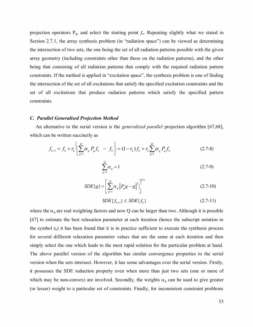
53
projection operators Pq, and select the starting point fo. Repeating slightly what we stated in
Section 2.7.1, the array synthesis problem (in “radiation space”) can be viewed as determining
the intersection of two sets, the one being the set of all radiation patterns possible with the given
array geometry (including constraints other than those on the radiation patterns), and the other
being that consisting of all radiation patterns that comply with the required radiation pattern
constraints. If the method is applied in “excitation space”, the synthesis problem is one of finding
the intersection of the set of all excitations that satisfy the specified excitation constraints and the
set of all excitations that produce radiation patterns which satisfy the specified pattern
constraints.
C. Parallel Generalised Projection Method
An alternative to the serial version is the generalized parallel projection algorithm [67,68],
which can be written succinctly as
11 1
(1 )Q Q
k k k q q k k k k k q q kq q
f f r P f f r f r P f
(2.7-8)
11
Q
q
q (2.7-9)
1 2
2
1
{ }Q
q q
q
SDE g P g g
(2.7-10)
1{ } { }k kSDE f SDE f (2.7-11)
where the q are real weighting factors and now Q can be larger than two. Although it is possible
[67] to estimate the best relaxation parameter at each iteration (hence the subscript notation in
the symbol rk) it has been found that it is in practice sufficient to execute the synthesis process
for several different relaxation parameter values that are the same at each iteration and then
simply select the one which leads to the most rapid solution for the particular problem at hand.
The above parallel version of the algorithm has similar convergence properties to the serial
version when the sets intersect. However, it has some advantages over the serial version. Firstly,
it possesses the SDE reduction property even when more than just two sets (one or more of
which may be non-convex) are involved. Secondly, the weights q can be used to give greater
(or lesser) weight to a particular set of constraints. Finally, for inconsistent constraint problems
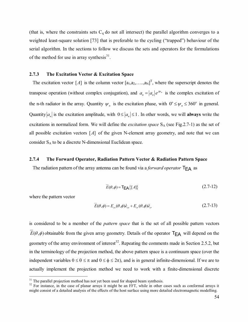
54
(that is, where the constraints sets Cq do not all intersect) the parallel algorithm converges to a
weighted least-square solution [73] that is preferable to the cycling (“trapped”) behaviour of the
serial algorithm. In the sections to follow we discuss the sets and operators for the formulations
of the method for use in array synthesis31
.
2.7.3 The Excitation Vector & Excitation Space
The excitation vector [ ]A is the column vector [a1,a2,…..,aN]T, where the superscript denotes the
transpose operation (without complex conjugation), and nj
n na a e
is the complex excitation of
the n-th radiator in the array. Quantity n is the excitation phase, with 0 360n o o in general.
Quantity na is the excitation amplitude, with 0 1na . In other words, we will always write the
excitations in normalized form. We will define the excitation space SA (see Fig.2.7-1) as the set of
all possible excitation vectors [ ]A of the given N-element array geometry, and note that we can
consider SA to be a discrete N-dimensional Euclidean space.
2.7.4 The Forward Operator, Radiation Pattern Vector & Radiation Pattern Space
The radiation pattern of the array antenna can be found via a forward operator TEA as
( , ) [ ]E A TEA (2.7-12)
where the pattern vector
ˆ ˆ( , ) ( , ) ( , )co co cr crE E e E e (2.7-13)
is considered to be a member of the pattern space that is the set of all possible pattern vectors
( , )E obtainable from the given array geometry. Details of the operator TEA will depend on the
geometry of the array environment of interest32
. Repeating the comments made in Section 2.5.2, but
in the terminology of the projection method, the above pattern space is a continuum space (over the
independent variables 0 and 0 2), and is in general infinite-dimensional. If we are to
actually implement the projection method we need to work with a finite-dimensional discrete
31 The parallel projection method has not yet been used for shaped beam synthesis. 32 For instance, in the case of planar arrays it might be an FFT, while in other cases such as conformal arrays it
might consist of a detailed analysis of the effects of the host surface using more detailed electromagnetic modelling.
55
representation of the pattern vector. So we sample the pattern at specific angles
1 2{ , ,......, ,...... }m M and define a forward operator TEA which maps SA directly onto a finite-
dimensional discrete pattern space SF. , namely
TEA{[A]} = [ED] = [ECO(1),ECO(2),..,ECO(M),ECR(1),ECR(2),.. , ECR(M) ]T (2.7-14)
We will thus write the forward operator as a matrix [ ]EAT , so that [ ] [ ][ ]D EAE T A . Note that
[ ]EAT will not be square because there are more pattern sampling points than array elements.
[ ]DE lies in the pattern space SF. If both co- and cross-polarised patterns are being considered,
then [ ]DE is a 2M-dimensional column vector as shown; if only co-polarised patterns enter into the
synthesis procedure then it is M-dimensional. In the former case forward operator [ ]EAT : SA SF
will be an N x 2M matrix, and in the latter case an N x M matrix. The forward operator [ ]EAT is
needed in the definition of certain projection operators in later sections.
In this thesis we will directly synthesise only the co-polarised pattern, so that we will denote
[ ]DE by [ ]COE , as already done in Section 2.5.2. The forward operator [ ]EAT is then that already
defined by (2.5-5)
2.7.5 The Backward (or Reverse, or Inverse) Operator
In addition to the forward operator which maps an element from the excitation space SA to an
element in the discrete radiation space SF we will, in the definition of certain projection operators to
be described below, require a backward (or reverse) operator TAE : SF SA which maps an
element of the discrete radiation space to an element in the excitation space SA. In the discrete finite-
dimensional spaces (that is, the matrix world) with which we are working this formally means that
we require 1[ ] [ ]AE EAT T . Since [ ]EAT is not a square matrix some form of generalised inverse
must be used.
One possibility is to use weighted least squares to determine the generalised inverse (and
hence the backward operator), namely
1
[ ] [ ] [ ][ ] [ ] [ ]H HAE EA EA EAT T W T T W
(2.7-15)
56
where [ ]W is a diagonal weighting vector, and superscript “H” indicates the conjugate transpose
operation. If [ ]W is selected to be the identity matrix the process reduces to conventional least
squares (also referred to as the maximum likelihood method). In executing the backward operator
the relative weights must be assigned to the weighting vector [ ]W . The main lobe region and each
sidelobe region can be assigned a regional weight according to their relative importance in a
particular application. In other words, the relative weights can be decreased at sampling angles
that are less important as far as precise satisfaction of the pattern constraints is concerned. This
will be demonstrated in Chapters 3 and 4.
Another possibility is to use the Moore-Penrose generalised inverse. This has the advantage
that highly efficient routines for its execution are readily available [74,75].
We have not yet defined the projection operators needed for the application of the synthesis
method under discussion. We are still in the process of defining various operators that will be
used in the eventual definition of such projection operators in Section 2.7.6 and Section 2.7.7,
and more completely in Chapter 3.
2.7.6 Operator Used to Implement Pattern Constraints
It is assumed that the pattern vector [ ]COE has been normalized. Then the operator33
that
enforces pattern constraints will be defined as
1 2
T
E CO CO CO CO CO MP E E E E E (2.7-16)
where
33 Note that this is also a projection operator. However, it is not one of the projection operators used directly in the
projection algorithm. But it will be used, along with the forward and reverse operators defined earlier, to construct
projection operators that are used directly in the algorithm.
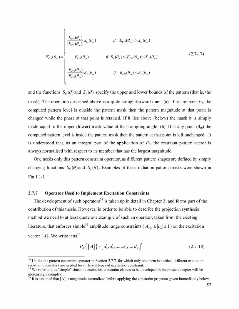
57
mm
m
m m m
mm
m
( )( ) ( ) ( )
( )
E ( ) ( ) ( ) ( ) ( )
( )( ) ( ) ( )
( )
COU m CO U m
CO
CO CO L m CO U m
COL m CO L m
CO
ES if E S
E
E if S E S
ES if E S
E
(2.7-17)
and the functions ( )US and ( )LS specify the upper and lower bounds of the pattern (that is, the
mask). The operation described above is a quite straightforward one : (a). If at any point m the
computed pattern level is outside the pattern mask then the pattern magnitude at that point is
changed while the phase at that point is retained. If it lies above (below) the mask it is simply
made equal to the upper (lower) mask value at that sampling angle. (b). If at any point (m) the
computed pattern level is inside the pattern mask then the pattern at that point is left unchanged. It
is understood that, as an integral part of the application of PE, the resultant pattern vector is
always normalised with respect to its member that has the largest magnitude.
One needs only this pattern constraint operator, as different pattern shapes are defined by simply
changing functions ( )US and ( )LS . Examples of these radiation pattern masks were shown in
Fig.1.1-1.
2.7.7 Operator Used to Implement Excitation Constraints
The development of such operators34
is taken up in detail in Chapter 3, and forms part of the
contribution of this thesis. However, in order to be able to describe the projection synthesis
method we need to at least quote one example of such an operator, taken from the existing
literature, that enforces simple35
amplitude range constraints ( min 1nA a ) on the excitation
vector [ ]A . We write it as36
1 1 2, ,...., ,...,T
A n NP A a a a a (2.7-18)
34 Unlike the pattern constraint operator in Section 2.7.7, for which only one form is needed, different excitation
constraint operators are needed for different types of excitation constraint. 35 We refer to it as "simple" since the excitation constraint classes to be developed in the present chapter will be
increasingly complex. 36 It is assumed that [A] is magnitude-normalized before applying the constraint projector given immediately below.
58
where
n min n
n nmin n min
n
a a 1
a aa
a
if A
A if A
(2.7-19)
The subscript “A” in 1AP denotes
37 that it is an operator that constrains the vector [A], as
opposed to the subscript “E” of EP in (2.7-16) that constrains the vector [ ]COE . Expression (2.7-
18) is just one of several operators that will be devised in Chapter 3 to apply various excitation
constraints. Note that the class of excitation constraint (2.7-18) does not place any constraint on
the excitation phases. All excitation amplitudes are constrained in a homogeneous manner over
the array aperture; the dynamic range allowed for an element at the centre of the array is the
same for one at the edge, and so on.
37 The “1” in the subscript identifies that it is only one of several excitation constraint projection operators that will
be used in this thesis, which will be uniquely identified as 2AP , 3AP , and so on. Only one pattern constraint projector
EP is needed though; but the masks that it enforces will change for different patterns shapes.
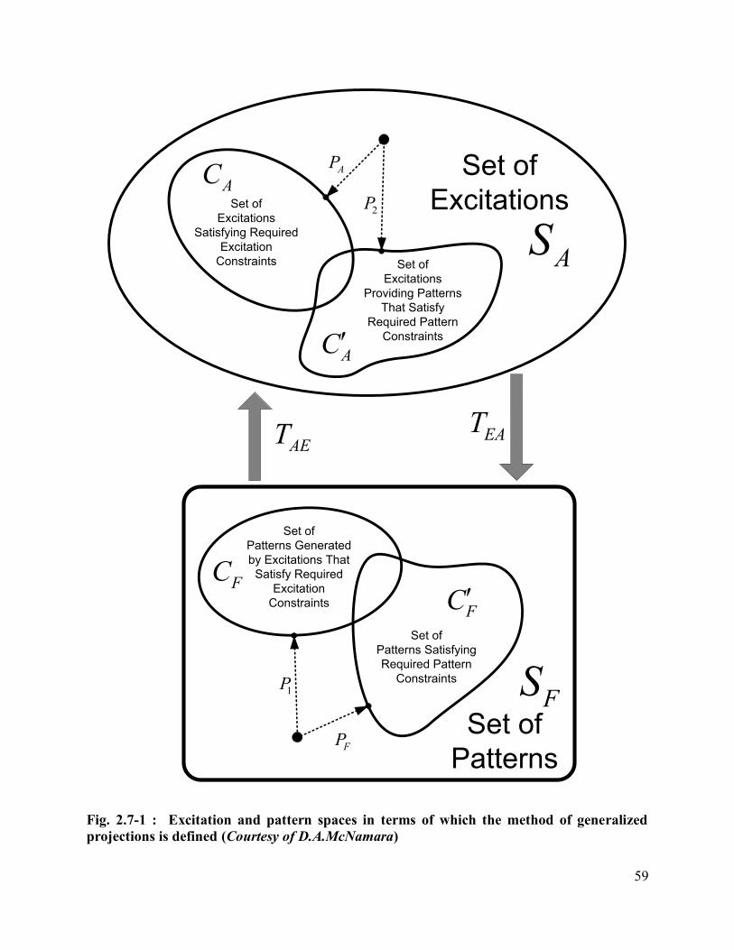
59
AET EAT
AS
FS
AC
AC
FC
FC
Set of
ExcitationsSet of
Excitations
Satisfying Required
Excitation
Constraints Set of
Excitations
Providing Patterns
That Satisfy
Required Pattern
Constraints
Set of
Patterns Satisfying
Required Pattern
Constraints
Set of
Patterns Generated
by Excitations That
Satisfy Required
Excitation
Constraints
Set of
Patterns
AP
FP
2P
1P
Fig. 2.7-1 : Excitation and pattern spaces in terms of which the method of generalized
projections is defined (Courtesy of D.A.McNamara)
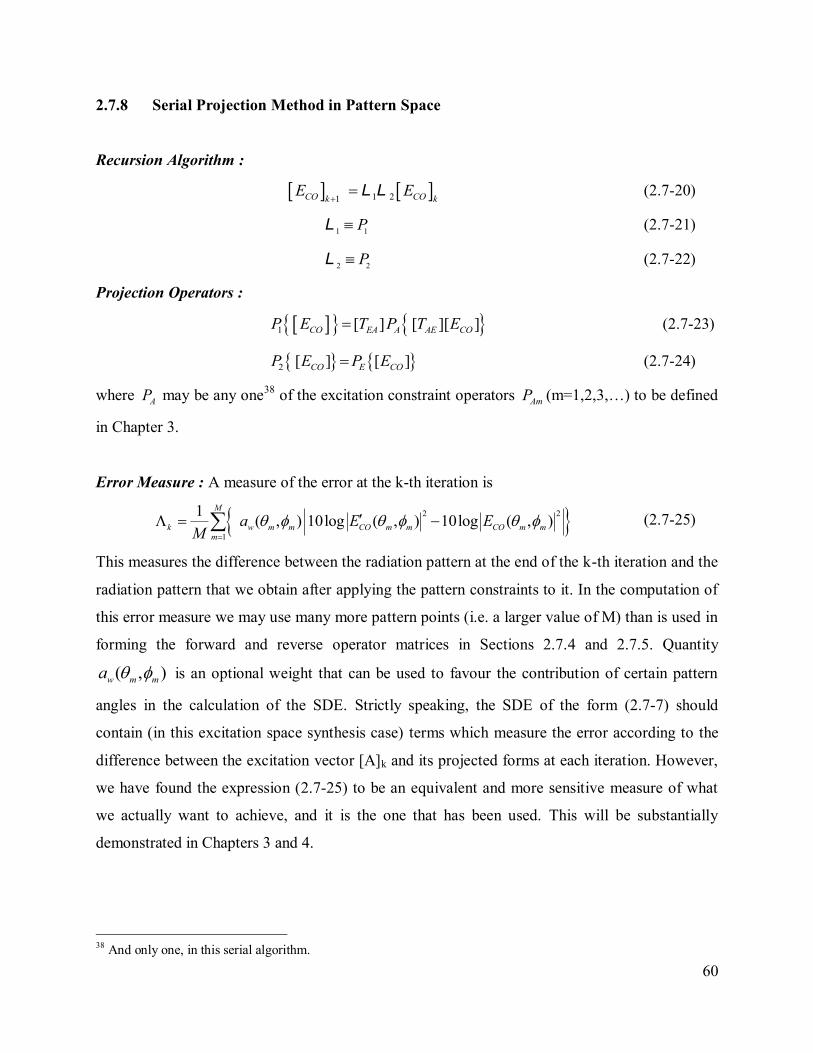
60
2.7.8 Serial Projection Method in Pattern Space
Recursion Algorithm :
1 21CO COk kE E
L L (2.7-20)
1 1
PL (2.7-21)
2 2
PL (2.7-22)
Projection Operators :
1 [ ] [ ][ ]CO EA A AE COP E T P T E (2.7-23)
2 [ ] [ ]CO E COP E P E (2.7-24)
where AP may be any one38
of the excitation constraint operators AmP (m=1,2,3,…) to be defined
in Chapter 3.
Error Measure : A measure of the error at the k-th iteration is
2 2
1
1( , ) 10log ( , ) 10log ( , )
M
k w m m CO m m CO m mm
a E EM
(2.7-25)
This measures the difference between the radiation pattern at the end of the k-th iteration and the
radiation pattern that we obtain after applying the pattern constraints to it. In the computation of
this error measure we may use many more pattern points (i.e. a larger value of M) than is used in
forming the forward and reverse operator matrices in Sections 2.7.4 and 2.7.5. Quantity
( , )w m m
a is an optional weight that can be used to favour the contribution of certain pattern
angles in the calculation of the SDE. Strictly speaking, the SDE of the form (2.7-7) should
contain (in this excitation space synthesis case) terms which measure the error according to the
difference between the excitation vector [A]k and its projected forms at each iteration. However,
we have found the expression (2.7-25) to be an equivalent and more sensitive measure of what
we actually want to achieve, and it is the one that has been used. This will be substantially
demonstrated in Chapters 3 and 4.
38 And only one, in this serial algorithm.
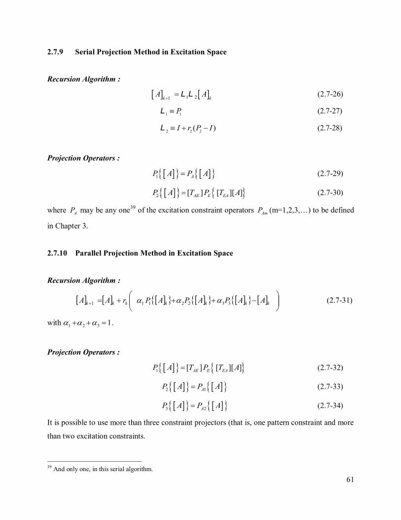
61
2.7.9 Serial Projection Method in Excitation Space
Recursion Algorithm :
1 21k kA A
L L (2.7-26)
1 1
PL (2.7-27)
2 2 2
( )I r P I L (2.7-28)
Projection Operators :
1 AP A P A (2.7-29)
2 [ ] [ ][ ]AE E EAP A T P T A (2.7-30)
where AP may be any one39
of the excitation constraint operators AmP (m=1,2,3,…) to be defined
in Chapter 3.
2.7.10 Parallel Projection Method in Excitation Space
Recursion Algorithm :
kkkkkkk AAPAPAPrAA 3322111 (2.7-31)
with 1321 .
Projection Operators :
1 [ ] [ ][ ]AE E EAP A T P T A (2.7-32)
2 1AP A P A (2.7-33)
3 2AP A P A (2.7-34)
It is possible to use more than three constraint projectors (that is, one pattern constraint and more
than two excitation constraints.
39 And only one, in this serial algorithm.
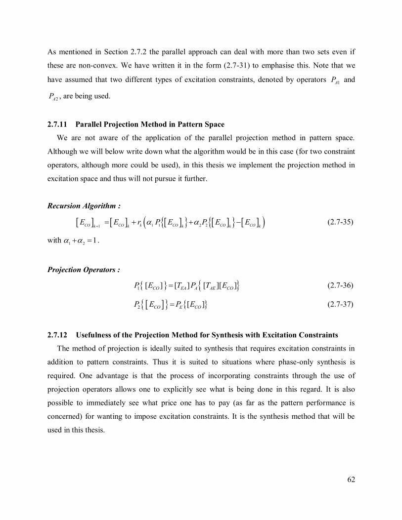
62
As mentioned in Section 2.7.2 the parallel approach can deal with more than two sets even if
these are non-convex. We have written it in the form (2.7-31) to emphasise this. Note that we
have assumed that two different types of excitation constraints, denoted by operators 1AP and
2AP , are being used.
2.7.11 Parallel Projection Method in Pattern Space
We are not aware of the application of the parallel projection method in pattern space.
Although we will below write down what the algorithm would be in this case (for two constraint
operators, although more could be used), in this thesis we implement the projection method in
excitation space and thus will not pursue it further.
Recursion Algorithm :
1 1 2 21CO CO k CO CO COk k k k kE E r P E P E E
(2.7-35)
with1 2
1 .
Projection Operators :
1 [ ] [ ] [ ][ ]CO EA A AE COP E T P T E (2.7-36)
2 [ ]CO E COP E P E (2.7-37)
2.7.12 Usefulness of the Projection Method for Synthesis with Excitation Constraints
The method of projection is ideally suited to synthesis that requires excitation constraints in
addition to pattern constraints. Thus it is suited to situations where phase-only synthesis is
required. One advantage is that the process of incorporating constraints through the use of
projection operators allows one to explicitly see what is being done in this regard. It is also
possible to immediately see what price one has to pay (as far as the pattern performance is
concerned) for wanting to impose excitation constraints. It is the synthesis method that will be
used in this thesis.
63
2.8 SELECTION OF STARTING POINTS FOR NUMERICAL SYNTHESIS
METHODS
A reasonable estimation of the starting values of the excitations (especially the excitataion
phases) is crucial when using the projection method for the excitation synthesis of shaped
beams40
. These values do not need to be precise (otherwise the synthesis would already have
been done!). But they must be such as to prevent the projection method from finding itself in a
trap41
.
One method that is widely used in all numerical optimization based synthesis methods takes
the average of the upper and lower pattern constraint masks42
at each pattern sampling point and
then finds the initial excitations by applying the backward operator. In other words, at each
pattern sampling angle (m) we can determine a pattern value given by the average value of the
upper and lower mask43
at that point as
mLmUmCO SSE 2
1)( (2.8-1)
and then form a pattern vector [ ]COE using these sampled values. It would represent a pattern with
the same phase at all pattern sampling angles. When this is operated on by the backward operator
we will obtain a set of excitations
[ ] [ ][ ]AE COA T E (2.8-2)
that can be used as starting values. This could be used for projection pattern synthesis methods too.
The disadvantage of this approach is that we force a particular phase distribution on the radiation
pattern from the onset of the iterations, and this can hinder convergence of the synthesis process.
One “trick” that sometimes overcomes this is to assign a random phase function or some other
phase function based on additional information about the problem. Another possibility is to use the
Woodward shaped beam synthesis method mentioned in Section 2.7.6 to find the starting
40 This is actually true for all numerical optimisation based synthesis techniques mentioned in Sections 2.5 and 2.6
as well. This fact is often not clearly stated in the literature, but one realises it all too soon when attempting to implement such techniques. 41 Equivalent to a numerical optimization algorithm finding itself stalled at a local optimum. 42 Shaped beam pattern masks will be discussed in detail in Section 2.9. 43 The upper and lower pattern masks US and LS are real quantities.

64
excitations44
. But this also suffers from the fact that the starting excitations are determined in a
manner that imposes a uniform array pattern phase. Some authors have used variants of
Woodward’s method, but these significantly complicate the problem. In Section 3.7 we will show
how an early continuous aperture distribution synthesis formulation, that is far too crude to be useful
in current engineering practice in its own right, can be manipulated to provide excellent starting
values for the projection synthesis method that, as stated in Section 2.7.12, is the technique of
choice in this thesis.
2.9 SHAPED BEAM PATTERN MASKS
2.9.1 Introductory Remarks
Brief discussions of shaped beam pattern requirements are scattered throughout the literature,
and when these are described this is done in a somewhat ad hoc fashion. We therefore thought it
worthwhile to come up with a structured way of talking about such patterns, in particular for the
three “canonical” shaped beams considered in this thesis - the flat-topped pattern, isoflux pattern
and cosecant pattern45
. We will systematize the process as one of first deciding on the idealised
pattern shape (which is non-realisable) and then proceeding to developing from this a pattern
mask (which will allow synthesis of a realizable array). Directly implementable forms of such
pattern masks do not appear to be written down in the literature reviewed, and so we provide this
in the present section. In order to connect this shaped beam material to what most of us are used
to, we briefly first state this process for the case of a pencil beam pattern.
2.9.2 Pencil Beam Pattern Mask
In many applications (eg. point-to-point line of sight communications) we wish an antenna to
radiate in a single direction and in no other. Such an idealized pencil beam antenna (for which
the direction of desired radiation is assumed to be = 0) would have the radiation pattern
shown in Fig.2.9-1. It is obviously not possible to obtain an antenna of finite size provide such a
44 We are of course not suggesting the use of Woodward’s method for the overall synthesis problem, since it is not able to enforce sidelobe or excitation constraints. 45 The techniques we develop to synthesize these cases are applicable to other radiation pattern shapes as well. We
have selected the above-mentioned three because we need to validate the methods on specific actual examples, and
these three are ones that are used in practice.
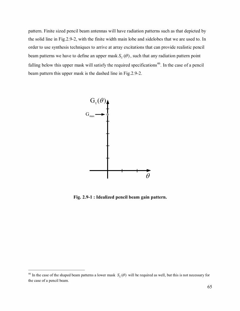
65
pattern. Finite sized pencil beam antennas will have radiation patterns such as that depicted by
the solid line in Fig.2.9-2, with the finite width main lobe and sidelobes that we are used to. In
order to use synthesis techniques to arrive at array excitations that can provide realistic pencil
beam patterns we have to define an upper mask ( )US , such that any radiation pattern point
falling below this upper mask will satisfy the required specifications46
. In the case of a pencil
beam pattern this upper mask is the dashed line in Fig.2.9-2.
tG ( )
maxG
Fig. 2.9-1 : Idealized pencil beam gain pattern.
46 In the case of the shaped beam patterns a lower mask ( )LS will be required as well, but this is not necessary for
the case of a pencil beam.
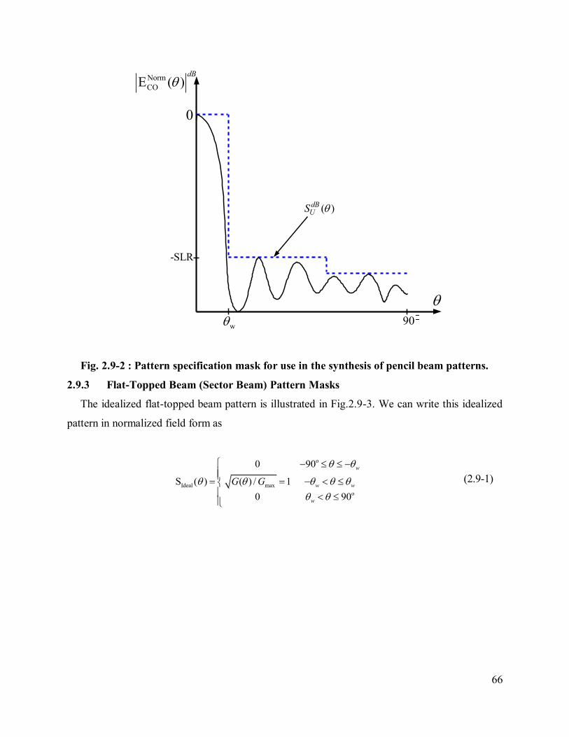
66
-SLR
w
90
Norm
COE ( )dB
0
( )dBUS
Fig. 2.9-2 : Pattern specification mask for use in the synthesis of pencil beam patterns.
2.9.3 Flat-Topped Beam (Sector Beam) Pattern Masks
The idealized flat-topped beam pattern is illustrated in Fig.2.9-3. We can write this idealized
pattern in normalized field form as
Ideal max
0 90
S ( ) ( ) / 1
0 90
w
w w
w
G G
o
o
(2.9-1)
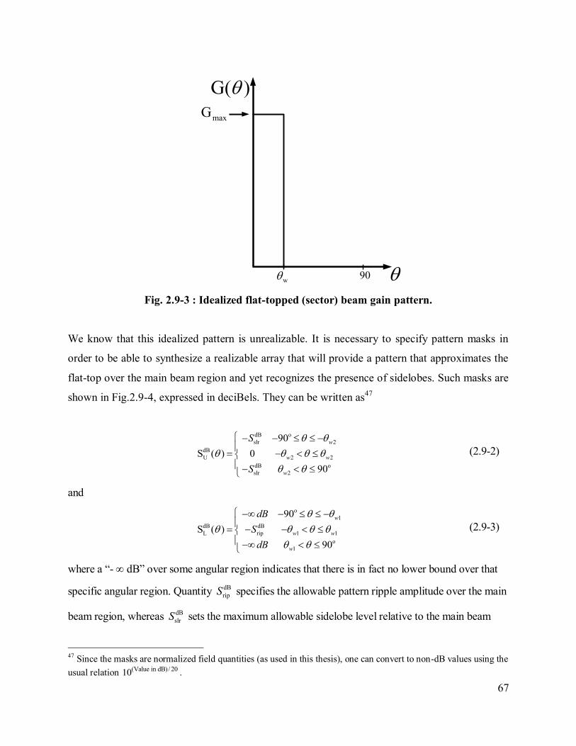
67
w 90
G( )
maxG
Fig. 2.9-3 : Idealized flat-topped (sector) beam gain pattern.
We know that this idealized pattern is unrealizable. It is necessary to specify pattern masks in
order to be able to synthesize a realizable array that will provide a pattern that approximates the
flat-top over the main beam region and yet recognizes the presence of sidelobes. Such masks are
shown in Fig.2.9-4, expressed in deciBels. They can be written as47
dB
slr 2
dB
U 2 2
dB
slr 2
90
S ( ) 0
90
w
w w
w
S
S
o
o
(2.9-2)
and
1
dB dB
L rip 1 1
1
90
S ( )
90
w
w w
w
dB
S
dB
o
o
(2.9-3)
where a “- dB” over some angular region indicates that there is in fact no lower bound over that
specific angular region. Quantity dB
ripS specifies the allowable pattern ripple amplitude over the main
beam region, whereas dB
slrS sets the maximum allowable sidelobe level relative to the main beam
47 Since the masks are normalized field quantities (as used in this thesis), one can convert to non-dB values using the
usual relation (Value in dB)/ 2010 .
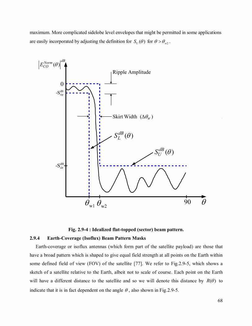
68
maximum. More complicated sidelobe level envelopes that might be permitted in some applications
are easily incorporated by adjusting the definition for ( )US for 2w .
dB
slr-S
0
w1w2 90
dB
rip-S
Skirt Width ( )W
Ripple Amplitude
( )dB
NormCOE
( )dBUS
( )dBLS
Fig. 2.9-4 : Idealized flat-topped (sector) beam pattern.
2.9.4 Earth-Coverage (Isoflux) Beam Pattern Masks
Earth-coverage or isoflux antennas (which form part of the satellite payload) are those that
have a broad pattern which is shaped to give equal field strength at all points on the Earth within
some defined field of view (FOV) of the satellite [77]. We refer to Fig.2.9-5, which shows a
sketch of a satellite relative to the Earth, albeit not to scale of course. Each point on the Earth
will have a different distance to the satellite and so we will denote this distance by ( )R to
indicate that it is in fact dependent on the angle , also shown in Fig.2.9-5.

69
0Earth Satellite
( )R
max 0( )R R
(0)H R
e
Earth Radius
6378kmR
Denotes an Arbitary Point on the Earth's Surface within the Satellite's FOV
Line Tangent to the Earth's Surface at
Fig. 2.9-5 : Sketch Illustrating Satellite-Earth Geometry for Derivation of the Shaped
Pattern Characteristics Required for an Isoflux Antenna (Courtesy of D.A.McNamara)
The power density at a point on the Earth depends on the path length R between that point
and the satellite, and on the atmospheric attenuation A along that path. The path length )(R can
be determined using the cosine rule to be
2 2( ) 2 ( )cose e e eR R R H R R H (2.9-4)
which reduces to
2 21 4[( / ) / ]sin ( / 2)]e eR H R H R H (2.9-
5)
where
90 (2.9-6)
and
1cos [(1 / )sin ]eH R (2.9-7)
Angle is the elevation angle of the satellite at the specific point on the Earth within the FOV.
It usually has a minimum value min , with atmospheric attenuation precluding use of the

70
communication link between points on the Earth and the satellite for whichmin . This defines
the maximum value of , namely
1
FOV minsin [ cos /( )]e eR R H (2.9-8)
for a point on the Earth at the edge of coverage (EOC), and the Earth-satellite distance is then at
its maximum value of max FOV( )R R . Note that FOV 0 , with 1
0 sin [ /( )]e eR R H . If the
point on the Earth is directly "below" the satellite (the sub-satellite point or nadir direction), so
that 0 o, then the Earth-satellite distance is at its minimum value of (0 )H R o that is the
orbital height of the satellite. In the case of geostationary (GEO) satellites 35786kmH and
hence FOV is less than 10◦. In the case of low-Earth-orbit (LEO) satellites the EOC angle FOV
can be more than o60 .
If ( )U is the radiation intensity function (that is, the radiation pattern) of the antenna, then
the power density at distance ( )R from the antenna is 2( ) ( ) ( )S R U . In order to have the
same power density at all points on the Earth we must have 0
( ) ( )S S
o for all values of
FOV . If atmospheric attenuation is neglected48
, this implies that
2 2
( ) (0 )
( ) (0 )
U U
R R
o
o (2.9-9)
which becomes
2
2
(0 )( ) ( )
UU R
H
o
(2.9-10)
The directivity function of this antenna is then
FOV FOV FOV
2
2
2
0 0 0 0
4 ( ) 4 ( ) 2 ( )( )
( )sin 2 ( )sin ( )sin
U U RD
U d d U d R d
(2.9-11)
Once the orbital height H and the minimum elevation angle min have been specified, expression
(2.9-13) can be evaluated using numerical integration to give the ideal isoflux directivity pattern.
48 Inclusion of atmospheric attenuation would be application specific (eg. it would depend on the operating
frequency), and could be incorporated in what follows. In Chapter 3 we wish to establish how isoflux-type patterns
could be synthesized under excitation constraints. Use of the zero atmospheric attenuation shape derived here will be
able to tell how well such methods work with isoflux-type patterns generally.

71
Although we are considering linear arrays, we earlier explained the applicability of linear array
synthesis to practical cylindrical lens antennas, and so use of the physical three-dimensional
directivity definition is relevant.
As an implementational detail, we note that the expression (2.9-11) has been evaluated using
the Matlab numerical integration routine QUADL49
. Examples of its application are shown in
Fig.2.9-6 for two different orbital heights.
49 The Matlab manual reports that routine QUADL approximates the integral of the integrand function to within an
error of 10-6 using high-order recursive Labatto adaptive quadrature.
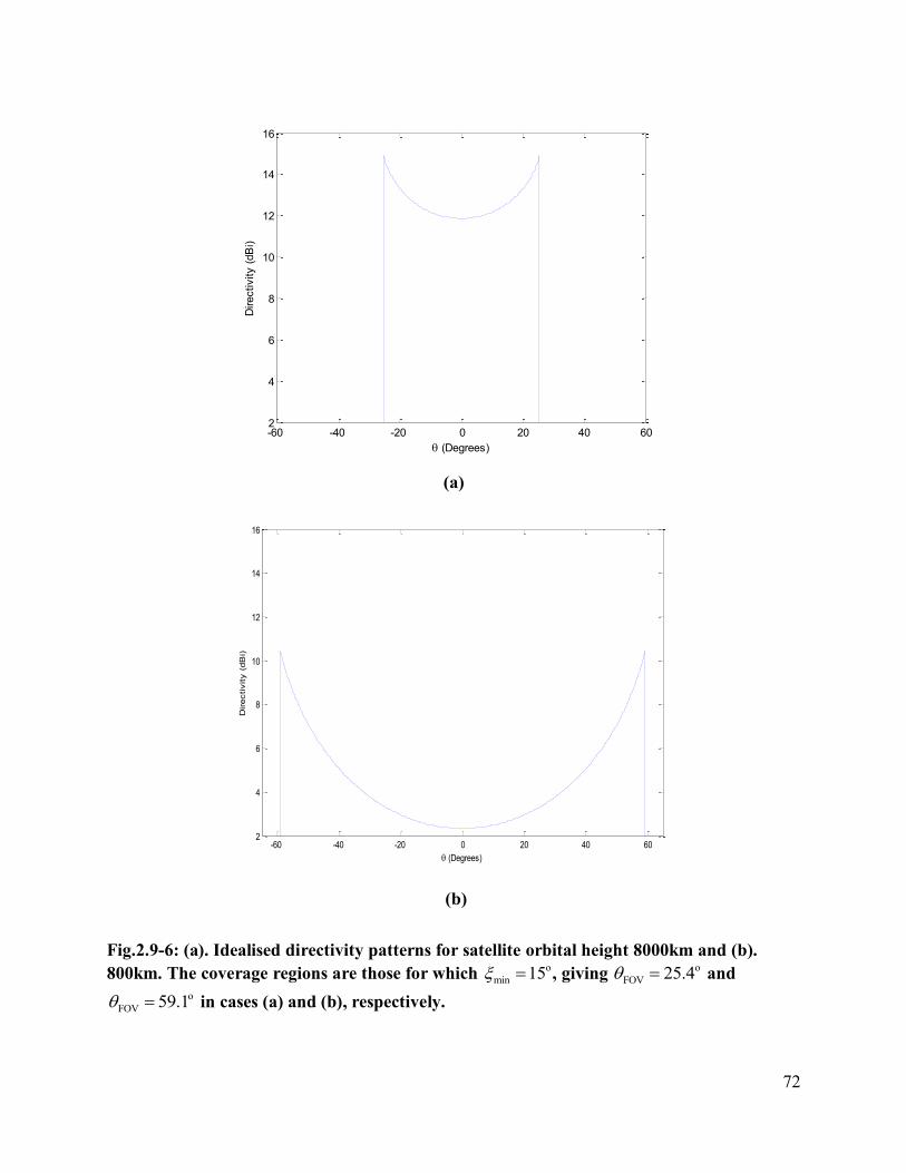
72
-60 -40 -20 0 20 40 602
4
6
8
10
12
14
16
(Degrees)
Directivity (
dB
i)
(a)
-60 -40 -20 0 20 40 602
4
6
8
10
12
14
16
(Degrees)
Directivity (
dB
i)
(b)
Fig.2.9-6: (a). Idealised directivity patterns for satellite orbital height 8000km and (b).
800km. The coverage regions are those for which min 15 o, giving FOV 25.4 o
and
FOV 59.1 o in cases (a) and (b), respectively.
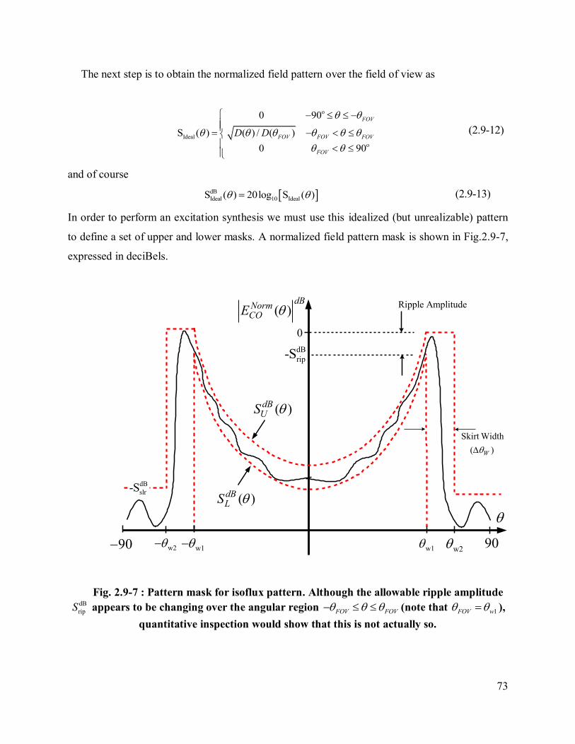
73
The next step is to obtain the normalized field pattern over the field of view as
Ideal
0 90
S ( ) ( ) / ( )
0 90
FOV
FOV FOV FOV
FOV
D D
o
o
(2.9-12)
and of course
dB
Ideal 10 IdealS ( ) 20log S ( ) (2.9-13)
In order to perform an excitation synthesis we must use this idealized (but unrealizable) pattern
to define a set of upper and lower masks. A normalized field pattern mask is shown in Fig.2.9-7,
expressed in deciBels.
w1
dB
rip-S
90
Skirt Width
( )W
( )dB
NormCOE
( )dBUS
( )dBLS
Ripple Amplitude
90
0
dB
slr-S
w2w2w1
Fig. 2.9-7 : Pattern mask for isoflux pattern. Although the allowable ripple amplitude dB
ripS appears to be changing over the angular region FOV FOV (note that 1FOV w ),
quantitative inspection would show that this is not actually so.
74
These masks can be written as
dB
slr 2
2 1
dB dBU Ideal 1 1
1 2
dB
slr 2
90
0
S ( ) S ( )
0
90
w
w w
w w
w w
w
S
S
o
o
(2.9-14)
and
2
2 1
dB dB dB dB dBL Ideal rip U rip 1 1
1 2
2
90
S ( ) S ( ) S ( )
90
w
w w
w w
w w
w
dB
dB
S S
dB
dB
o
o
(2.9-15)
where, as before, a “- dB” over some angular region indicates that there is in fact no lower bound
over that specific angular region. Quantity dB
ripS specifies the allowable pattern ripple amplitude over
the main beam region, whereas dB
slrS sets the maximum allowable sidelobe level relative to the main
beam maximum.
Execution of the synthesis procedure might fail to provide this required pattern shape. It is
important to realise that this might not be the fault of the synthesis process. Since the idealized
pattern is derived from directivity considerations the “user” of the synthesis procedures might
have chosen an array size that is too small or too large. It may be necessary to re-run the
synthesis procedure for arrays of different size and examine the trends. As in most cases of
antenna engineering one cannot simply “crank the handle”. Although synthesis procedures are
most useful tools, insight on the part of the designer remains essential.
2.9.5 Cosecant-Squared Beam Pattern Masks
Cosecant-squared beams have been required for air surveillance radars, ground-mapping
radars, and wireless networks. We consider the air surveillance application first, and refer to
Fig.2.6-8 that depicts an airport radar antenna and an approaching aircraft. The radar cross-
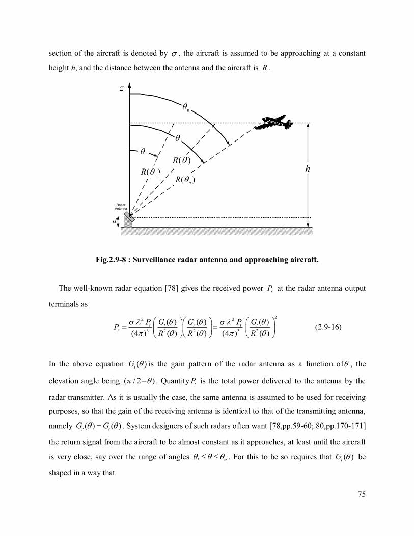
75
section of the aircraft is denoted by , the aircraft is assumed to be approaching at a constant
height h, and the distance between the antenna and the aircraft is R .
u
Radar
Antenna
( )R
( )R
d
h
z
( )uR
Fig.2.9-8 : Surveillance radar antenna and approaching aircraft.
The well-known radar equation [78] gives the received power rP at the radar antenna output
terminals as
22 2
3 2 2 3 2
( ) ( )( )
(4 ) ( ) ( ) (4 ) ( )
t t t trr
P G P GGP
R R R
(2.9-16)
In the above equation ( )tG is the gain pattern of the radar antenna as a function of , the
elevation angle being ( / 2 ) . Quantity tP is the total power delivered to the antenna by the
radar transmitter. As it is usually the case, the same antenna is assumed to be used for receiving
purposes, so that the gain of the receiving antenna is identical to that of the transmitting antenna,
namely ( ) ( )r tG G . System designers of such radars often want [78,pp.59-60; 80,pp.170-171]
the return signal from the aircraft to be almost constant as it approaches, at least until the aircraft
is very close, say over the range of angles l u . For this to be so requires that ( )tG be
shaped in a way that
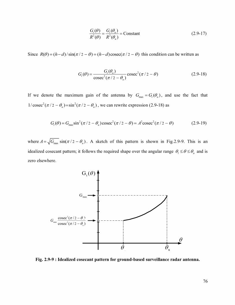
76
2 2
( ) ( )Constant
( ) ( )
t t u
u
G G
R R
(2.9-17)
Since 2 2( ) ( ) / sin( / ) ( )cosec( / )R h d h d this condition can be written as
2
22
2
( )( ) cosec ( / )
cosec ( / )
t ut
u
GG
(2.9-18)
If we denote the maximum gain of the antenna by max ( )t uG G , and use the fact that
2 22 21/ cosec ( / ) sin ( / )u u , we can rewrite expression (2.9-18) as
2 2 2 2
max 2 2 2( ) sin ( / )cosec ( / ) cosec ( / )t uG G A (2.9-19)
where max 2sin( / )uA G . A sketch of this pattern is shown in Fig.2.9-9. This is an
idealized cosecant pattern; it follows the required shape over the angular range l u and is
zero elsewhere.
tG ( )
u
maxG
2
max 2
2
2
cosec ( / )
cosec ( / )u
G
Fig. 2.9-9 : Idealized cosecant pattern for ground-based surveillance radar antenna.

77
The wireless network cell in Fig.2.6-10 is considered next. The Friis transmission equation
[78] gives the received power at the receive antenna terminals as
2
2 2
( ) ( )
(4 ) ( )
t t rr
P G GP
R
(2.9-20)
The user receive antennas are low directivity antennas, and in this analysis we assume they are
isotropic. This implies that ( ) 1rG , and hence that (2.9-20) becomes
2
2 2
( )
(4 ) ( )
t tr
P GP
R
(2.9-21)
If wireless network designers wish the received signal to be the same at all receive positions in a
cell [81] over the range of angles l u then we need ( )tG be shaped such that
2 2
( ) ( )Constant
( ) ( )
t tG G
R R
l
l
(2.9-22)
which at once means that
2 2max
2 2
( )( ) cosec cosec
cosec cosec
tt
G GG
l
l l
(2.9-23)
since ( ) ( )cosecR h d . This pattern is sketched in Fig.2.9-10.
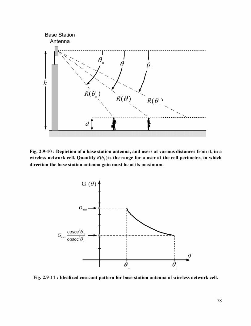
78
u
Base Station
Antenna
( )R ( )R ( )uR
d
h
Fig. 2.9-10 : Depiction of a base station antenna, and users at various distances from it, in a
wireless network cell. Quantity ( )R l is the range for a user at the cell perimeter, in which
direction the base station antenna gain must be at its maximum.
tG ( )
u
maxG
2
max 2
cosec
cosecu
G
Fig. 2.9-11 : Idealized cosecant pattern for base-station antenna of wireless network cell.
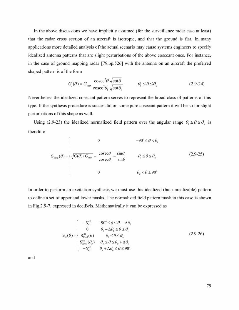
79
In the above discussions we have implicitly assumed (for the surveillance radar case at least)
that the radar cross section of an aircraft is isotropic, and that the ground is flat. In many
applications more detailed analysis of the actual scenario may cause systems engineers to specify
idealized antenna patterns that are slight perturbations of the above cosecant ones. For instance,
in the case of ground mapping radar [79,pp.526] with the antenna on an aircraft the preferred
shaped pattern is of the form
2
max 2
cosec cot( )
cosec cott uG G
l
l l
(2.9-24)
Nevertheless the idealized cosecant pattern serves to represent the broad class of patterns of this
type. If the synthesis procedure is successful on some pure cosecant pattern it will be so for slight
perturbations of this shape as well.
Using (2.9-23) the idealized normalized field pattern over the angular range l u is
therefore
maxIdeal
0 90
sincosec( ) /S ( )
cosec sin
0 90
l
l u
u
G G
o
l
l
o
(2.9-25)
In order to perform an excitation synthesis we must use this idealized (but unrealizable) pattern
to define a set of upper and lower masks. The normalized field pattern mask in this case is shown
in Fig.2.9-7, expressed in deciBels. Mathematically it can be expressed as
dB
slr
dBU Ideal
dB
Ideal
dB
slr
90
0
S ( ) S ( )
S ( )
90
u
u u u u
u u
S
S
o
l l
l l l
l
o
(2.9-26)
and
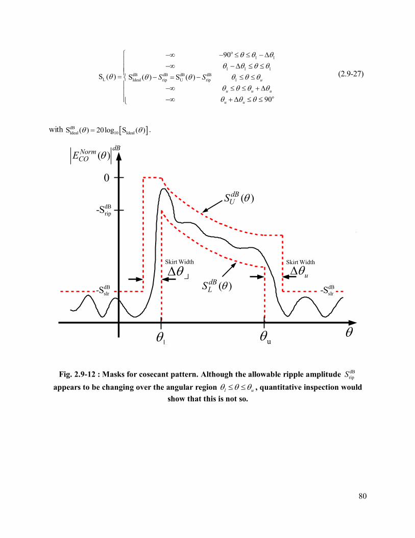
80
dB dB dB dBL Ideal rip U rip
90
S ( ) S ( ) S ( )
90
u
u u u
u u
S S
o
l l
l l l
l
o
(2.9-27)
with dB
Ideal 10 IdealS ( ) 20log S ( ) .
u
udB
slr-S
dB
rip-S
Skirt Width
( )dB
NormCOE
( )dBUS
( )dBLS
Skirt Width
dB
slr-S
0
Fig. 2.9-12 : Masks for cosecant pattern. Although the allowable ripple amplitude dB
ripS
appears to be changing over the angular region l u , quantitative inspection would
show that this is not so.
81
2.10 CONCLUSIONS
We began this chapter by recognizing the enormous amount of work that has been published
on excitation synthesis in general, but were able to restrict that part of it which we would be
reviewing. This was made possible by selecting only those portions that are applicable to what
we wish to achieve in this thesis, or were the forerunners upon which such methods are based. It
allowed us to classify existing synthesis techniques into four broad classes, namely classical
techniques, those based directly on general numerical optimisation algorithms, those that can be
formulated as convex programming problems, and ones based on the method of projections.
Having argued why generalised projection methods would be used in the present work, we
delved into such methods in some detail, in order to lay the groundwork for Chapter 3 and
Chapter 4, where these methods are extended and applied to the specific problems at hand.
Although not the major contribution of this thesis, this tutorial-like elucidation of the method
of projections in a manner that takes it beyond the mathematical framework in which it is usually
couched, into an applications-oriented format, does not appear to be available elsewhere. We
have also presented, in one place, a systematic derivation and explanation of three specific types
of shaped beam, namely sector-beams, isoflux beams and cosecant-squared beams, which are
used in practice. This, along with the careful formulation of a way to specify pattern constraints
for projection methods that will lead to such beam shapes that has been given, we have not found
in other publications.
82
2.11 REFERENCES FOR CHAPTER 2
[1] R. C. Hansen, Phased Array Antennas (Wiley, 1998).
[2] C. A. Balanis, Antenna Theory (Wiley, 2005) Fig.6.6.
[3] P. Kildal, “Aperture efficiency and line feed phase center of parabolic cylindrical
reflector antenna”, IEEE Trans. Antennas Propagat., Vol.32, No.6, pp.553-561, June
1984.
[4] M. Leung, J. S. Kot and B. B. Jones, “Wideband dual polarized line feed development for
a cylindrical reflector radio telescope”, IEEE Int. AP-S Symp. Digest, pp.1929-1932,
2007.
[5] N. Gagnon, A. Petosa & D. A. McNamara, "Electrically Thin Free-Standing Phase and
Amplitude Shifting Surface for Beam Shaping Applications", Microwave & Optical
Technology Letters, Vol.54, No.7, pp.1566-1571, July 2012.
[6] M. T. Ma, Theory and Application of Antenna Arrays, (John Wiley and Sons, 1974).
[7] D. K. Cheng, "Optimisation techniques for antenna arrays", Proc. IEEE, Vol. 59, pp.
1664-1674, Dec. 1971.
[8] R. L. Pritchard, "Optimum directivity patterns for linear point arrays", J. Acoustical Soc.
Amer., Vol.25, No.5, pp. 879-891, Sept.1953.
[9] Y. T. Lo, S. W. Lee and Q. H. Lee, "Optimisation of directivity and signal-to-noise ratio of
an arbitrary antenna array", Proc. IEEE, Vol. 54, No. 8, pp. 1033-1045, Aug. 1966.
[10] R. C. Hansen, Chaps.9 & 10. in : A.W.Rudge et.al.(Edits.), The Handbook of Antenna
Design, Vol.2 (Peter Peregrinus Ltd., 1982).
[11] C. L. Dolph, "A current distribution for broadside arrays which optimises the relationship
between beam width and side-lobe level", Proc. IRE, Vol. 34, pp. 335-348, June 1946.
[12] R. C. Hansen, "Fundamental limitations in antennas", Proc. IEEE, Vol. 69, No. 2, pp.
170-182, Feb. 1981.
[13] G. Meinardus, Approximation of Functions : Theory and Numerical Methods (Springer-
Verlag, 1967).
[14] R. E. Collin & F. J. Zucker, Antenna Theory, Part I (McGraw-Hill, 1969).
[15] H. J. Riblet, "Discussion on 'A current distribution for broadside arrays which optimises the
relationship between beam width and sidelobe level'.", Proc. IRE, Vol. 35, pp. 489-492,
June 1947.
83
[16] R. C. Hansen, “Array pattern control and synthesis”, Proc. IEEE (Special Issue on
Antennas), Vol.80, pp.141-151, Jan.1992.
[17] R. C. Hansen (Edit.), Microwave Scanning Antennas Vol.I (Academic Press, 1964).
[18] R. J. Mailloux, Phased Array Antenna Handbook (Artech House, 1994).
[19] R. L. Pritchard, “Optimum directivity patterns for linear point arays”, J. Acoustical Soc.
Am., Vol.25, No.5, pp.879-891, Sept.1953.
[20] R. H. DuHamel, “Optimum patterns for endfire arrays”, Proc. IRE, Vol.41, pp.652-659,
1953.
[21] D. A. McNamara, “An Exact Formulation for the Synthesis of Broadside Chebyshev
Arrays of 2N Elements with Inter-Element Spacing d < /2”, Microwave & Optical Tech.
Letters, Vol.48, No.3, pp.457-463, March 2006
[22] R. J. Stegen, “Gain of Tchebycheff arrays”, IRE Trans. Antennas Propagat., Vol.8,
pp.629-631, Nov.1960.
[23] R. C. Hansen, "Aperture efficiency of Villeneuve n arrays", IEEE Trans. Antennas Prop.,
Vol. AP-33, No.6, pp. 668-669, June 1985.
[24] A. T. Villeneuve, "Taylor patterns for discrete arrays", IEEE Trans. Antennas Prop., Vol.
AP-32, No. 10, pp.1089-1093, Oct. 1984.
[25] D. A. McNamara, "Generalised Villeneuve n -distribution", IEE Proc., Vol.136, No.3,
pp.245-249, June 1989.
[26] P. M. Woodward, “Method of calculating the field over a plane aperture required to
produce a given polar diagram”, J.IEEE, Pt.IIA, Vol.93, pp.1554-1558, 1947.
[27] R. S. Elliott, Antenna Theory and Design (Prentice-Hall, 1981).
[28] K. Milne, “Synthesis of power radiation patterns for linear array antennas”, IEE Proc.,
Pt.H, Vol.134, No.3, pp.285-296, June 1987.
[29] H. J. Orchard, R. S. Eliott, and G. J. Stern, “Optimising the synthesis of shaped antenna
patterns”, IEE Proc. Microwave Antennas Propagat., Vol.132, pp.63-68, 1985.
[30] B. D. Carlson & D. Willner, “Antenna pattern synthesis using weighted least squares”, IEE
Proc., Vol.139, Pt.H, pp.11-16, Feb.1992.
84
[31] L. I. Vaskelainen, “Iterative least-squares synthesis methods for conformal array antennas
with optimized polarization and frequency properties”, IEEE Antennas Propagat., Vol.45,
pp.1179-1185, July 1997.
[32] L. I. Vaskelainen, “Constrained least-squares optimization in conformal array antenna
synthesis”, IEEE Antennas Propagat., Vol.55, No.3, pp.859-867, March 2007.
[33] L. I. Vaskelainen, "Phase synthesis of conformal array antennas", IEEE Trans. Antennas
Propagat., Vol.48, No.6, pp.987-991, June 2000.
[34] J. F. DeFord and O. P. Gandhi, "Phase-only synthesis of minimum peak sidelobe patterns
for linear and planar arrays", IEEE Trans. Anten. Propag. 36(2):191–201 (Feb. 1988).
[35] F. Ares-Pena, "Applications of genetic algorithms and simulated annealing to some antenna
problems, in Electromagnetic Optimization by Genetic Algorithms, Y.Rahmat-Samii and E.
Michielssen (Edits.), pp. 119–155 (Wiley, 1999).
[36] J. M. Johnson and Y. Rahmat-Samii, "Genetic algorithms in engineering electromagnetics",
IEEE Anten. Propag. Mag. 39(4):7–21 (Aug. 1997).
[37] R. L. Haupt, "An introduction to genetic algorithms for electromagnetics", IEEE Anten.
Propag. Mag. 37(2):7–15 (April 1995).
[38] R. Haupt, "Comparison between genetic and gradient-based optimization algorithms for
solving electromagnetics problems", IEEE Trans. Magn. 31(3):1932–1935 (May 1995).
[39] R. L. Haupt, Antenna Arrays: A Computational Approach (Wiley, 2010).
[40] R. L. Haupt and D. Werner, Genetic Algorithms in Electromagnetics (Wiley, 2007).
[41] R. L. Haupt, "Optimum quantized low sidelobe phase tapers for arrays", Electron. Lett.
31(14):1117–1118 (July 1995).
[42] D. W. Boeringer and D. H. Werner, "Adaptive mutation parameter toggling genetic
algorithm for phase-only array synthesis", Electron. Lett. 38(25):1618–1619 (Dec. 2002).
[43] D. W. Boeringer, D. H. Werner, and D. W. Machuga, "A simultaneous parameter
adaptation scheme for genetic algorithms with application to phased array synthesis", IEEE
Trans. Anten. Propag. 53(1):356–371 (Jan. 2005).
[44] K. K. Yan and Y. Lu, "Sidelobe reduction in array-pattern synthesis using genetic
algorithm", IEEE Trans. Anten. Propag. 45(7):1117–1122 (July 1997).
[45] D. Marcano and F. Duran, "Synthesis of antenna arrays using genetic algorithms", IEEE
Anten. Propag. Mag. 42(3):12–20 (June 2000).
85
[46] D. W. Boeringer and D. H. Werner, "Particle swarm optimization versus genetic algorithms
for phased array synthesis", IEEE Trans. Anten. Propag. 52(3):771–779 (March 2004).
[47] O. M. Bucci, M. D’Urso & T. Isernia, “Some facts and challenges in array antenna
synthesis”, 19th Int. Conf. Applied Electromagnetics and Communications (ICECom),
Sept.2007.
[48] O. M. Bucci, M. D’Urso & T. Isernia, “Exploiting convexity in array antenna synthesis
problems”, Proc. IEEE Radar Conf. (RadarCon), Rome, Italy, 2008.
[49] R. R. Kurth, “Optimization of array performance subject to multiple power pattern
constraints”, IEEE Trans. Antennas Propagat., Vol. AP-22, No.1, pp.103-105, Jan.1974.
[50] O. Einarsson, “Optimization of planar arrays”, IEEE Trans. Antennas Propagat., Vol. AP-27,
No.1, pp.86-92, Jan.1979.
[51] K. Hirasawa, “The application of a biquadratic programming method for phase-only
optimization of antenna arrays”, IEEE Trans. Antennas Propagat., Vol. 36, No.11, pp.1545-
1550, Nov.1988.
[52] B. P. Ng, M. H. Er and C. Kot, “A flexible array synthesis method using quadratic
programming”, IEEE Trans. Antennas Propagat., Vol. AP-41, No.11, pp.1541-1550,
Nov.1993.
[53] H. Lebret and S. Boyd, “Antenna array pattern synthesis via convex optimization”, IEEE
Trans. Signal Processing, Vol. AP-45, No.3, pp.526-532, March 1997.
[54] T. Isernia and G. Panariello, “Optimal focusing of scalar fields subject to arbitrary upper
bounds”, Electronics Letters, Vol.34, No.2, pp.162-164, Jan.1998.
[55] T. Isernia, P. Di Iorio and F. Soldovieri, “An effective approach for the optimal focusing of
array fields subject to arbitrary upper bounds”, IEEE Trans. Antennas Propagat., Vol. 48,
No.12, pp.1837-1847, Dec.2000.
[56] O. M. Bucci, L. Caccavale and T. Isernia, “Optimal far-field focusing of uniformly spaced
arrays subject to arbitrary upper bounds in nontarget directions”, IEEE Trans. Antennas
Propagat., Vol. 50, No.11, pp.1539-1553, Nov. 2002.
[57] R. Torrealba, D. H. Covarubbias and M. Panduro, “Analysis of robustness for convex
optimization applied to array antenna pattern synthesis”, J. Computer Science, Vol.4,
No.12, pp.1036-1041, 2008.
[58] P. Rocca, L. Manica, R. Azaro and A. Massa, “A hybrid approach to the synthesis of
subarrayed monopulse linear arrays”, IEEE Trans. Antennas Propagat., Vol. 57, No.1,
pp.280-283, Jan.2009.
86
[59] S. Prasad, “Generalized array pattern synthesis by the method of alternating orthogonal
projections”, IEEE Trans. Antennas Propagat., Vol. AP-28, No.3, pp.328-332, May 1980.
[60] A. Levi & H. Stark, “Image restoration by the method of generalised projections with
application to restoration from magnitude”, J.Opt.Soc. Am., Pt.A, Vol.1, No.9, pp.932-
943, Sept.1984.
[61] G. T. Poulton, “Antenna power pattern synthesis using method of successive projections”,
Electronics Lett., Vol.22, No.20, pp.1042-1043, Sept.1986.
[62] O. M. Bucci, G. Franceschetti, G. Mazzarella & G. Panariello, “Intersection approach to
array pattern synthesis”, IEE Proc., Vol.137, Pt.H, No.6, pp.349-357, Dec.1990.
[63] O. M. Bucci & G. D’Elia, “Power synthesis of reconfigurable conformal arrays with
phase-only control”, IEE Proc.-Microw. Antennas Propag., Vol.145, No.1, pp.131-136,
Feb.1998.
[64] E. Botha & D. A. McNamara, “Conformal array synthesis using alternating projections,
with maximum likelihood estimation used in one of the projection operators”, Electronics
Lett., Vol.29, No.20, pp.1733-1734, Sept.1993.
[65] O. M. Bucci, G. D’Elia & G. Romito, “Power synthesis of conformal arrays by a
generalised projection method”, IEE Proc.-Microw. Antennas Propag., Vol.142, No.6,
pp.467-471, Dec.1995.
[66] E. Botha, J. Joubert & D. A. McNamara, “Alternative Formulation & Applications
Aspects of the Generalised Projection Method for Array Antenna Synthesis”,
International Journal of RF and Microwave Computer-Aided Engineering, Vol.19, No.6,
pp.657-668, Nov.2009.
[67] H. Stark & Y. Yang, Vector Space Projections : A Numerical Approach to Signal and
Image Processing, Neural Nets, and Optics (Wiley, 1998).
[68] P. L. Combettes, “On the numerical robustness of the parallel projection method in signal
synthesis”, IEEE Signal Processing Letters, Vol.8, No.2, pp.45-47, Feb.2001.
[69] Y. Censor, N. Cohen, T. Kotzer & J. Shamir, “Summed square distance error reduction
by simultaneous multiprojections and applications”, Applied Mathematics &
Computation, Vol.126, pp.157-179, 2002.
[70] G. Pierra, “Decomposition through formalisation in a product space”, Math.
Programming, Vol.28, pp.96-115, Jan.1984.
[71] T. Swierczynski & D. A. McNamara, “The Solution of ‘Switched Element’ Array
Synthesis Problems Using the Parallel Generalised Projection Algorithm”, Microwave &
Optical Technology Letters, Vol.40, No.6, pp.465-471, March 2004.

87
[72] R. J. Marks, “Alternating Projections onto Convex Sets”, Chapter 14 in P.A.Jansson (Edit.),
Deconvolution of Images and Spectra (Academic Press, 1997) Second Edition.
[73] P. L. Combettes, “Inconsistent signal feasibility problems : Least-squares solutions in a
product space”, IEEE Trans. Signal Processing, Vol.42, pp.2955-2966, Nov.1994.
[74] IMSL Math Library, Routine LSGRR.
[75] Routine pinv, MATLAB, The Mathworks Inc., Natick, Massachussetts, USA.
[76] E. Botha, J. Joubert & D .A. McNamara, “The Selection of Starting Points for Array
Synthesis Using the Method of Generalised Projections”, URSI National Radio Science
Meeting Digest, Boston, Massachusetts, USA, July 2001, p.85.
[77] L. J. Ricardi, “Satellite Antennas”, Chapter 36 in : R.C. Johnson, Antenna Engineering
Handbook (3rd
Edition), McGraw-Hill, 1993.
[78] G. Thiele and W. Stutzman, Antenna Theory & Design (Wiley, 1998) Chap.8
[79] M. I. Skolnik, Introduction to Radar Systems (McGraw-Hill, 1962).
[80] S. Drabowitch, A. Papiernik, H. D. Griffiths, J. Encinas & B. L. Smith, Modern Antennas
(Springer, 2005) 2nd
Edition.
[81] E. Holzman, “Pillbox antenna design for millimeterwave base-station applications”, IEEE Antennas & Propagation Magazine, Vol.45, No.1, pp.27-37, Feb.2003.
88
CHAPTER 3
Modified Method of Projections for Transmission
Coefficient Synthesis of Cylindrical Printed Lens Antennas
3.1 GOALS
A number of reasons were identified in Section 1.1 as to why printed lenses for shaped beams
have been found to not perform as well as expected. It is believed that if the range of amplitude
and phase values of the printed lens element transmission coefficients could be made to satisfy
certain constraints then, for reasons of practical implementation, it might be possible to improve
such performance. These constraints include the use of a pre-dominantly phase-based synthesis
to have less back-scatter from the input surface of the lens. Another possibility is to not require
that just any transmission coefficients be dictated by the synthesis process, but only ones that are
members of some database. In this chapter we develop a synthesis method that makes such
constraints possible. It is based on the method of generalized projections.
Section 3.2 discusses a feed field model needed for the developments in this chapter. In
Section 3.3 we derive a forward operator that allows the projection method to operate in the lens
element transmission coefficient space; in other words the transmission coefficients are directly
the variables in the synthesis process. Section 3.4 gives an appropriate reverse operator.
Projection operators that allow a variety of transmission coefficient constraints to be applied are
provided in Sections 3.5 through 3.8. Some are adaptations of ones quoted in the existing
literature, albeit expressed directly in terms of the transmission coefficient. Those in Sections 3.7
and 3.8 have not been used by others; they are new. Both a serial and a parallel projection
synthesis algorithm are stated in Section 3.9. These will be implemented in Chapter 4. A parallel
projection algorithm has not yet been used for shaped beam synthesis by anyone; we will
demonstrate some of its advantages over the serial form in Section 4.3. We mentioned in Section
2.7 that a reasonable estimation of starting values for the element phases is essential when using
the projection method for the synthesis of shaped beams in order to avoid so-called traps. It was
also noted that there is no general scheme that will provide such starting points. In Section 3.10
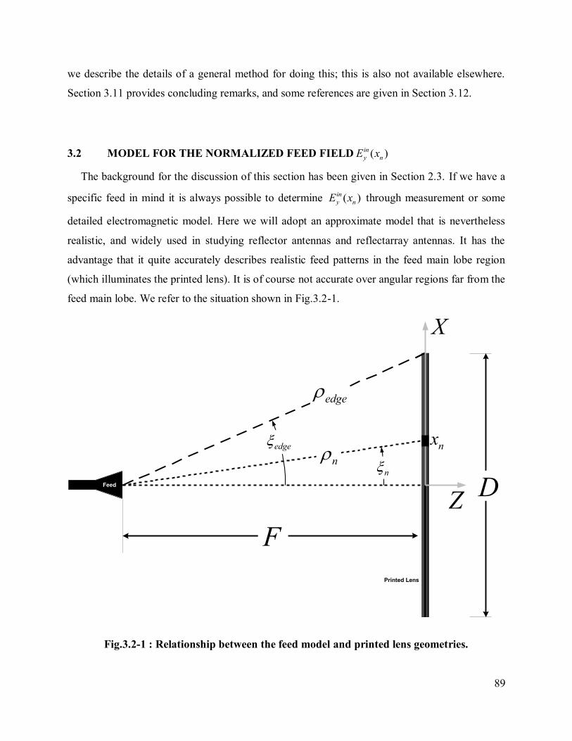
89
we describe the details of a general method for doing this; this is also not available elsewhere.
Section 3.11 provides concluding remarks, and some references are given in Section 3.12.
3.2 MODEL FOR THE NORMALIZED FEED FIELD ( )in
y nE x
The background for the discussion of this section has been given in Section 2.3. If we have a
specific feed in mind it is always possible to determine ( )in
y nE x through measurement or some
detailed electromagnetic model. Here we will adopt an approximate model that is nevertheless
realistic, and widely used in studying reflector antennas and reflectarray antennas. It has the
advantage that it quite accurately describes realistic feed patterns in the feed main lobe region
(which illuminates the printed lens). It is of course not accurate over angular regions far from the
feed main lobe. We refer to the situation shown in Fig.3.2-1.
F
n
edge
edge
n
DFeed
Printed Lens
Z
X
nx
Fig.3.2-1 : Relationship between the feed model and printed lens geometries.

90
Simple geometry allows us to write
2 2
n nx F (3.2-1)
1tan ( / )n nx F (3.2-2)
1 1/ 2 1tan tan
2( / )edge
D
F F D
(3.2-3)
and 2 2( / 2)edge D F (3.2-4)
Using a raised-cosine feed pattern model [1], we have
( ) cos ( )njk
q
y n n
n
eE x
(3.2-5)
This implies that
max 1
yEF
(3.2-6)
and so the normalised feed field on the input surface of the printed lens is
max
( )( ) cos ( )
njky nin q
y n n
ny
E x eE x F
E
(3.2-7)
If we wish to have a feed illumination taper50
of 0 dBC say, this means we need to select m such
that
0 20log ( / 2) 20log cos ( )in q
y edge
edge
FC E D
(3.2-8)
50 This means that, since the normalised feed field on axis is 0dB , that at the edge of the lens is 0 dBC .
91
which gives
0( / 20) log ( / )
log cos( )
edge
edge
C Fq
(3.2-9)
For example, if we have a printed lens with aperture dimension D = 152.4 mm with an
/ 0.5F D . This means that F = 76.2mm. Thus we have 45edge o and 107.76mmedge . If
we want 0 10dBC , then we must have q = 2.4.
If we wish to examine the synthesis process (that follows) without the feed effects we can
simply set m = 0 and make F large relative to D. The determination of ( )in
y nE x could be more
sophisticated than the raised cosine feed model used here. It could be extracted from the output
of a detailed computational electromagnetics model of the feed, or it could be found from a near-
field measurement of the feed fields back-projected to the plane with which the printed less input
surface eventually coincides.
3.3 FORWARD OPERATOR WITH LENS ELEMENT TRANSMISSION
COEFFICIENTS AS SYNTHESIS VARIABLES
Recall that the radiation pattern analysis model in expression (2.2-19) is
1
( ) ( )eN
CO n n
n
E a F
(3.3-1)
where
sin( , ) njkx
nF e (3.3-2)
Using expression (2.3-9) from Section 2.3 that relates the effective complex excitation of the n-th
lens element (at the output surface of the lens) to the complex transmission coefficient nb of the
element and the feed field ( )in
y nE x incident on the n-th element (at the input surface of the lens),
to the allows us to rewrite (3.3-1) in the form
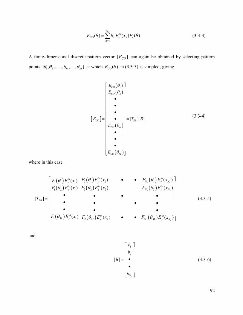
92
1
( ) ( ) ( )eN
in
CO n y n n
n
E b E x F
(3.3-3)
A finite-dimensional discrete pattern vector [ ]COE can again be obtained by selecting pattern
points 1 2{ , ,......, ,...... }m M at which ( )COE in (3.3-3) is sampled, giving
1
2
[ ][ ]
CO
CO
CO EB
CO m
CO M
E
E
E T B
E
E
(3.3-4)
where in this case
2 1 2 11 1 1
2 2 2 21 2 1
1 1 2 2
( ) ( )( )
( ) ( )( )
[ ]
( ) ( ) ( )
e e
e e
e
in ininy N y Ny
in inin
y N y Ny
EB
in in inM y M y N M y N
F E x F E xF E x
F E x F E xF E x
T
F E x F E x F E x
(3.3-5)
and
1
2
[ ]
eN
b
b
B
b
(3.3-6)
93
is vector of lens element transmission coefficients.
By defining the new forward operator in (3.3-5) we are now able to use the vector of element
transmission coefficients [ ]B directly in the projection synthesis technique as the synthesis
variable. Any constraint projection operators used in the application of the method are now
directly constraints on the transmission coefficients, which is what we really want. One “sees”
the transmission coefficient amplitudes and phases explicitly. The synthesis process is brought a
step closer to the practical design issues. It is possible to examine the effect of the feed pattern
beamwidth (in the present model, by changing the value of the index m), and hence the effect of
the amplitude and phase taper across the input surface of the lens. One can also observe the
influence of the F/D ratio on the range of transmission coefficient values required.
It is understood that the definition of [ ]EBT implicitly includes normalisation of the resultant
pattern vector [ ]COE .
3.4 REVERSE OPERATOR WITH LENS ELEMENT TRANSMISSION
COEFFICIENTS AS SYNTHESIS VARIABLES
The reverse operator will be some generalized inverse of the forward operator, and so we can
use the result in Section 2.7.5 to write
1
[ ] [ ] [ ][ ] [ ] [ ]H HBE EB EB EBT T W T T W
(3.4-1)
which is the same as that used in [2], except here it will map from the pattern space directly to
the transmission coefficient space.
94
3.5 PROJECTION OPERATORS FOR TRANSMISSION COEFFICIENT
AMPLITUDE DYNAMIC RANGE RESTRICTIONS
3.5.1 Excitation Amplitude Dynamic Range Restriction
This was extracted from [2], and has already been defined in Section 2.7.8 where, in order to
explain the various projection synthesis algorithm types, we needed to define at least one
excitation constraint operator in order to show in concrete terms what is meant by such an
operator. However, here we write it in terms of the element transmission coefficient vector. In
order to be able to easily distinguish between the various transmission coefficient constraint
operators we will introduce, we will call the present constraint operator 1BP ; subsequent operators
will be labeled BmP for m = 2,3,…,7.
Dynamic range is defined as the ratio of the maximum transmission coefficient magnitude to
the minimum transmission coefficient magnitude, namely max min/B B . We will always normalize
the transmission coefficient magnitudes before applying the dynamic ratio constraint, and so we
will can use max 1B . Then a projection operator that enforces an amplitude dynamic range
constraint ( min nb 1B ) on the transmission coefficient vector [ ]B is
1 1 2, ,...., ,...,e
T
B n NP B b b b b (3.5-1)
where51
n min n
n nmin n min
n
b b 1
b bb
if B
B if Bb
(3.5-2)
This class of transmission coefficient constraint does not place any constraint on the
transmission coefficient phases. The operation described (3.5-1) can be described in words as
follows :
- The transmission coefficient ( nb ) of each of the 1,2,....., en N elements is examined in
turn.
51 We have shown the bounds as being the same for all elements. They could of course be set such they are
dependent on the element index. In other words the bounds could be different for each element. Similar comments
can be made for the remaining transmission coefficient constraints that will be discussed.
95
- If the magnitude of nb is larger than the maximum value it is set equal to the maximum
value, but its phase is left unaltered.
- If the magnitude of nb lies within the bounds maxB and minB then na is left unaltered in both
amplitude and phase.
- If the magnitude of nb is smaller than the minimum value it is set equal to the minimum
value, but its phase is left unaltered.
- It is understood that, as an integral part of the application of 1BP the resultant excitations
are always normalized with respect to that which has the largest magnitude.
3.5.2 Excitation Restricted to be Symmetric in Amplitude and Phase
2 1 2, ,...., ,...,e
T
B n NP B b b b b (3.5-3)
where
- 1
1 b
2 en n N nb b (3.5-4)
The operation described (3.5-3) can be described in words as follows :
- The complex transmission coefficient of each of the 1,2,....., en N elements is obtained by
taking the average of each nb and the transmission coefficient of the corresponding element
(namely eN -n+1b ) in the other half of the array.
- This gives a projected set of excitations that is symmetrical in both amplitude and phase.
Expression (3.5-3) is applicable whether the number of array elements eN is even or odd. We
devised this transmission coefficient constraint projection operator because we initially thought it
would be needed to ensure symmetry when symmetrical shaped beam patterns are synthesized.
In the numerical experiments conducted (to be reported in Chapter 4) we observed that this is not
needed if the starting values of the transmission coefficients to be discussed in Section 3.10 are
themselves symmetrical. So use of this projection operator was actually not needed; we have
nevertheless documented it here for the sake of completeness.

96
3.5.3 Transmission coefficient Restricted to be Purely Real
3 1 2, ,...., ,...,e
T
B n NP B b b b b (3.5-5)
where
Re( )n n nb b sign b (3.5-6)
where n( )bRe means “real part of”, and the sign function performs precisely what it’s names
says, namely take the sign of its argument.
The operation described (3.5-5) can be described in words as follows :
- The magnitude of each complex transmission coefficient is retained.
- The transmission coefficient phase is set to 0 if the phase of nb is such that
( 90 ,90 )nb o o .
- The transmission coefficient phase is set to -180 if the phase of nb is such that
(90 ,270 )nb o o .
- This gives a projected set of transmission coefficients that is real.
We devised this transmission coefficient constraint projection operator because in the literature
review we noticed that real distributions are often required for pencil beam patterns; such a
projection operator would be useful if using the synthesis methods described here for pencil
beam work. However, we did not utilize this projection operator in the work of this thesis as
(with the benefit of hindsight) it is inappropriate for shaped beam synthesis.
97
3.6 PROJECTION OPERATORS FOR TRANSMISSION COEFFICIENT
AMPLITUDE & PHASE RESTRICTIONS
If, as illustrated in Fig.3.6-1, we wish to bound the range of both the amplitude and phase of the
transmission coefficients within intervals [Bmin,1] and [min,max], respectively, then52
4 1 2, ,...., ,...,e
T
B n NP B b b b b (3.6-1)
where the nb are found by applying first the rule
max
min
n n max n max
n n min n max
n n min n min
b cos( )
b b
b cos( )
j
j
b e if b
if b
b e if b
(3.6-2)
followed by the rule
n min n
n nmin n min
n
b b 1
b bb
if B
B if Bb
(3.6-3)
Observe that one determines the set of nb first, and then the set of nb . In other words the phase
constraint is applied first and then the amplitude constraint, The order is important. Swapping them
around would not result in a projection onto the correct set of constrained transmission coefficients
[3]. The operation described (3.6-1) can be described in words as follows:
- The transmission coefficient ( nb ) of each of the 1,2,....., en N elements is examined in
turn.
- The phase of each nb is restrained to the range max min[ , ] .
- The amplitude dynamic range restriction is then applied to the resultant transmission
coefficient (namely nb ) as in Section 3.5.1.
52 As always, the element excitation magnitudes must be normalized prior to implementation of the constraint rule
that follows. Note that this constraint operator was described in [3]; here we express it in terms of the element
transmission coefficient vector [B].
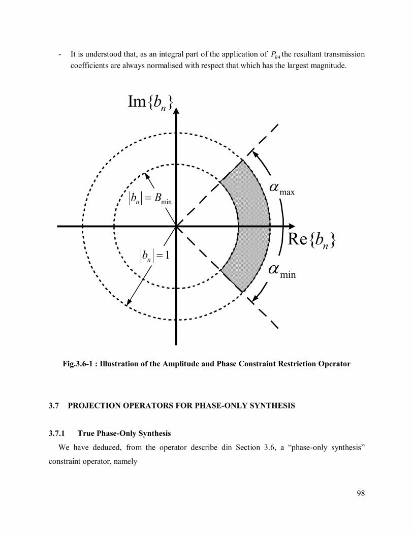
98
- It is understood that, as an integral part of the application of 4BP the resultant transmission
coefficients are always normalised with respect that which has the largest magnitude.
Im{ }nb
Re{ }nb
minnb B
1nb
max
min
Fig.3.6-1 : Illustration of the Amplitude and Phase Constraint Restriction Operator
3.7 PROJECTION OPERATORS FOR PHASE-ONLY SYNTHESIS
3.7.1 True Phase-Only Synthesis
We have deduced, from the operator describe din Section 3.6, a “phase-only synthesis”
constraint operator, namely
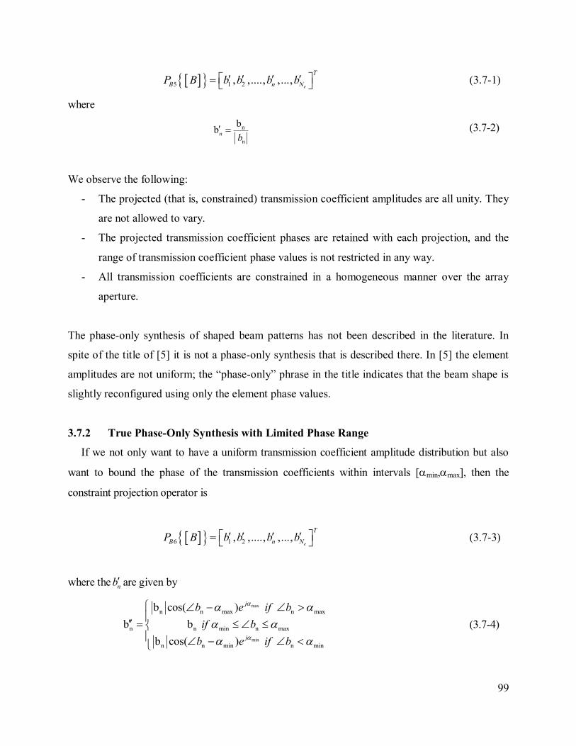
99
5 1 2, ,...., ,...,e
T
B n NP B b b b b (3.7-1)
where
n
n
bbn
b (3.7-2)
We observe the following:
- The projected (that is, constrained) transmission coefficient amplitudes are all unity. They
are not allowed to vary.
- The projected transmission coefficient phases are retained with each projection, and the
range of transmission coefficient phase values is not restricted in any way.
- All transmission coefficients are constrained in a homogeneous manner over the array
aperture.
The phase-only synthesis of shaped beam patterns has not been described in the literature. In
spite of the title of [5] it is not a phase-only synthesis that is described there. In [5] the element
amplitudes are not uniform; the “phase-only” phrase in the title indicates that the beam shape is
slightly reconfigured using only the element phase values.
3.7.2 True Phase-Only Synthesis with Limited Phase Range
If we not only want to have a uniform transmission coefficient amplitude distribution but also
want to bound the phase of the transmission coefficients within intervals [min,max], then the
constraint projection operator is
6 1 2, ,...., ,...,e
T
B n NP B b b b b (3.7-3)
where the nb are given by
max
min
n n max n max
n n min n max
n n min n min
b cos( )
b b
b cos( )
j
j
b e if b
if b
b e if b
(3.7-4)
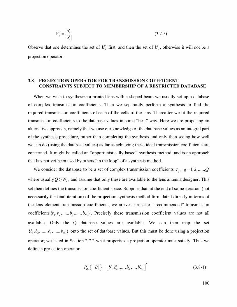
100
n
n
bb
bn
(3.7-5)
Observe that one determines the set of nb first, and then the set of nb , otherwise it will not be a
projection operator.
3.8 PROJECTION OPERATOR FOR TRANSMISSION COEFFICIENT
CONSTRAINTS SUBJECT TO MEMBERSHIP OF A RESTRICTED DATABASE
When we wish to synthesize a printed lens with a shaped beam we usually set up a database
of complex transmission coefficients. Then we separately perform a synthesis to find the
required transmission coefficients of each of the cells of the lens. Thereafter we fit the required
transmission coefficients to the database values in some ”best” way. Here we are proposing an
alternative approach, namely that we use our knowledge of the database values as an integral part
of the synthesis procedure, rather than completing the synthesis and only then seeing how well
we can do (using the database values) as far as achieving these ideal transmission coefficients are
concerned. It might be called an “opportunistically based” synthesis method, and is an approach
that has not yet been used by others “in the loop” of a synthesis method.
We consider the database to be a set of complex transmission coefficients q , 1,2,.....,q Q
where usually eQ N , and assume that only these are available to the lens antenna designer. This
set then defines the transmission coefficient space. Suppose that, at the end of some iteration (not
necessarily the final iteration) of the projection synthesis method formulated directly in terms of
the lens element transmission coefficients, we arrive at a set of “recommended” transmission
coefficients 1 2{ , ,....., ,....., }en Nb b b b . Precisely these transmission coefficient values are not all
available. Only the Q database values are available. We can then map the set
1 2{ , ,....., ,....., }en Nb b b b onto the set of database values. But this must be done using a projection
operator; we listed in Section 2.7.2 what properties a projection operator must satisfy. Thus we
define a projection operator
7 1 2, ,...., ,...,e
T
B n NP B b b b b (3.8-1)
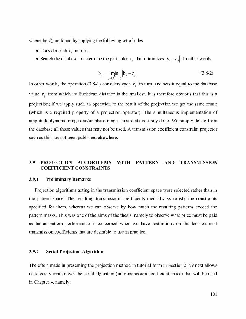
101
where the nb are found by applying the following set of rules :
Consider each nb in turn.
Search the database to determine the particular q that minimizes n qb . In other words,
{ n
1,2,.....,
b min bn q
q Q
(3.8-2)
In other words, the operation (3.8-1) considers each nb in turn, and sets it equal to the database
value q from which its Euclidean distance is the smallest. It is therefore obvious that this is a
projection; if we apply such an operation to the result of the projection we get the same result
(which is a required property of a projection operator). The simultaneous implementation of
amplitude dynamic range and/or phase range constraints is easily done. We simply delete from
the database all those values that may not be used. A transmission coefficient constraint projector
such as this has not been published elsewhere.
3.9 PROJECTION ALGORITHMS WITH PATTERN AND TRANSMISSION
COEFFICIENT CONSTRAINTS
3.9.1 Preliminary Remarks
Projection algorithms acting in the transmission coefficient space were selected rather than in
the pattern space. The resulting transmission coefficients then always satisfy the constraints
specified for them, whereas we can observe by how much the resulting patterns exceed the
pattern masks. This was one of the aims of the thesis, namely to observe what price must be paid
as far as pattern performance is concerned when we have restrictions on the lens element
transmission coefficients that are desirable to use in practice,
3.9.2 Serial Projection Algorithm
The effort made in presenting the projection method in tutorial form in Section 2.7.9 next allows
us to easily write down the serial algorithm (in transmission coefficient space) that will be used
in Chapter 4, namely:
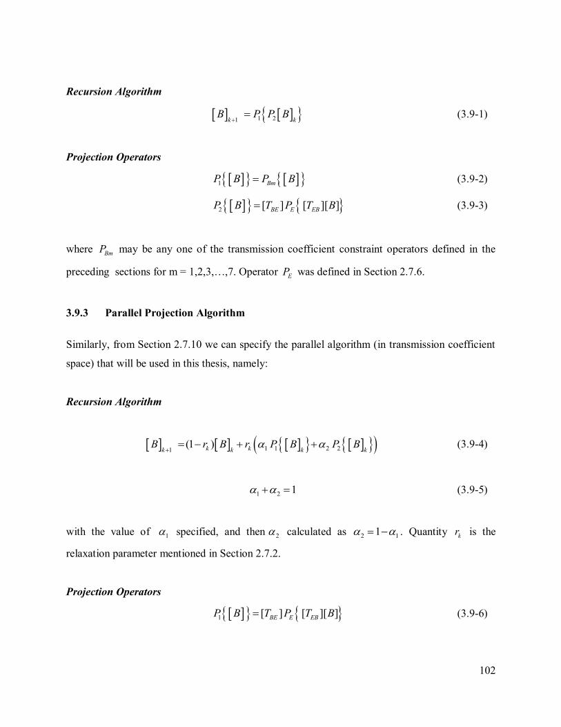
102
Recursion Algorithm
1 21k kB P P B
(3.9-1)
Projection Operators
1 BmP B P B (3.9-2)
2 [ ] [ ][ ]BE E EBP B T P T B (3.9-3)
where BmP may be any one of the transmission coefficient constraint operators defined in the
preceding sections for m = 1,2,3,…,7. Operator EP was defined in Section 2.7.6.
3.9.3 Parallel Projection Algorithm
Similarly, from Section 2.7.10 we can specify the parallel algorithm (in transmission coefficient
space) that will be used in this thesis, namely:
Recursion Algorithm
1 1 2 21(1 )k kk k k k
B r B r P B P B
(3.9-4)
1 2 1 (3.9-5)
with the value of 1 specified, and then 2 calculated as 2 11 . Quantity kr is the
relaxation parameter mentioned in Section 2.7.2.
Projection Operators
1 [ ] [ ][ ]BE E EBP B T P T B (3.9-6)
103
2 1 2, ,...., ,...,e
T
Bm n NP B P B b b b b (3.9-7)
3.10 STARTING VALUE ESTIMATION OF THE EXCITATION PHASES FOR
PROJECTION SYNTHESIS OF SHAPED BEAM PATTERNS
3.10.1 General Considerations
We explained in Section 2.7 that a reasonable estimation of starting values of the excitation
phases is essential when using the projection method for the excitation synthesis of shaped
beams. It was also noted that there is no general scheme that will provide such starting points.
However, we have in this work found that, for linear arrays, an approximate analytical technique
published more than 30 years ago [6,7] can serve this purpose quite satisfactorily. The technique
itself was published as a synthesis method in its own right, but would no longer be considered
appropriate for excitation synthesis purposes, since it is not able to impose even sidelobe
constraints (let alone excitation constraints). Its use as a possible means of obtaining starting
points for numerically based synthesis methods has been suggested by others, but no details have
been given on how to do this for specific shaped beams. We will demonstrate how it can be used
to rapidly provide starting excitation phase values for superior modern synthesis techniques such
as the method of projections. It is a good example of how earlier analytical methods can be
fruitfully used in novel ways to make modern numerically-based approaches more usable.
Whenever a new beam shape is required there is some minor analytical work needed on the part
of the engineer. Although this might be considered a disadvantage, the benefit is that one can
perform such derivations for a class of beam shapes once, and then very rapidly generate starting
phase values for any size array by simply solving a resulting differential equation numerically.
We show that this can be easily done using Matlab-based routines irrespective of the array size.
The reader is referred to [6,7] for the background to the method. We will here summarise the
procedure, and how we have applied it in this work53
:
A continuous linear source of length 2L is assumed to be lying on the x-axis, with L x L .
53 The notation used will be that of this thesis rather than that in references [6,7].
104
The amplitude distribution along the linear source is denoted by ( )A x , and is assumed to be
known. We have found, through the copious numerical experimentation of which the results in
Chapter 4 are a sample, that taking ( ) 1A x gives suitable starting values for the projection
synthesis method to proceed for the three shaped beams considered.
The goal is to find the phase distribution ( )x along the linear source in order to obtain a
radiation pattern described in normalised field form by ( )normF over the angular range
/ 2 / 2 .
Instead of using x and directly, the formulation uses normalised coordinates. These are
defined as
/ 1 1x L (3.10-1)
and
sin 1 1u u (3.10-2)
The first step is to evaluate
2 2
1
1
2 2
1
( ) ( )
( )
( ) ( )
x
L
L
L
A x dx A d
g
A x dx A d
(3.10-3)
where /x L has been used as a normalised dummy variable.
The second step is to use the ideal required pattern to evaluate
2
1
12
1
( )
( )
( )
u
norm
norm
F d
h u
F d
(3.10-4)
The third step is to equate ( )h u and ( )g , namely
( ) ( )h u g (3.10-5)
and use this to obtain an expression for variable ( )u , in other words an expression for the
normalised pattern angle u in terms of the normalised position on the linear source.
105
The fourth step is to use the expression for ( )u in the differential equation
( ) 2( ) 1 1
dLu
d
(3.10-6)
whose solution gives the required phase distribution ( ) of the continuous source. Phase is
always a relative quantity, and so without loss of generality we can use
0( ) 0
(3.10-7)
as the “initial condition” . In this thesis the above ordinary differential equation is solved using a
variable step Runge-Kutta method as implemented in the MATLAB routine ODE45 except for
the one instance for which the solution can be found in closed form.
The starting values of the excitation phases for the linear array of discrete elements is then
obtained by a simple sampling of the continuous starting phase distribution. It is well-known that
such direct sampling of continuous distributions does not provide a linear array with exactly the
same pattern as that of the continuous source. Indeed, even if the goal were actually the synthesis
of a continuous linear source the approach described here would not be considered sufficient, as
inspection of the results in [6,7] would show. But since we simply wish to have a set of “warm”
starting values that will be changed by the actual synthesis procedure none of the above two
issues need to concern us here. The values of the sampling points nx , in other words the array
element locations, are given in Section 2.3. The phase values ( )nx at these points are found
from the solution of the ordinary differential equation (3.10-6) by evaluating ( )n with
1 dn-N- 2N Elements
2 L
dn-N-1 2N+1 Elements
L
n
(3.10-8)
and
n nx L (3.10-9)
In what follows we will simply write this as ( )nx .
Finally, the starting transmission coefficient values can be found as / ( )in
n n y nb a E x .
However, we have found that it is even sufficient to use the starting na values directly for the
starting values of nb .
106
3.10.2 Flat-Topped Patterns : Estimation of the Starting Values of the Excitation
Phases
A. Idealized Pattern
Flat-topped pattern constraints were shown in Section 2.6.3. The flat-topped pattern is defined
over the range o ou u u , where 1coso wu , 1w is defined in Fig.2.9-4 in Section 2.9.3. The
normalized field pattern amplitude is equal to unity over the interval o ou u u and is zero
elsewhere. So we can write the normalized ideal flat-topped beam pattern as
0
0 0
0
0 1
( ) 1
0 1
norm
u u
F u u u u
u u
(3.10-10)
B. General Case
Using (3.10-1) the expression (3.10-4) becomes
0
0
0
2
0
2 0
( )
( )2
( )
a
b
a
u u
norm
u u
u u
norm
u u
F d du u
h uu
F d d
(3.10-11)
and so we can write
0
0
( )2
u ug
u
(3.10-12)
and hence
0( ) 2 ( ) 1u u g (3.10-13)
Expression (3.10-6) then allows us to write the differential equation as
0
( ) 22 ( ) 1 1 1
dLu g
d
(3.10-14)
Using the normalized dummy variable is /x L , we have ( ) ( )in
yA E , within
yE defined in
Section 2.3. Thus
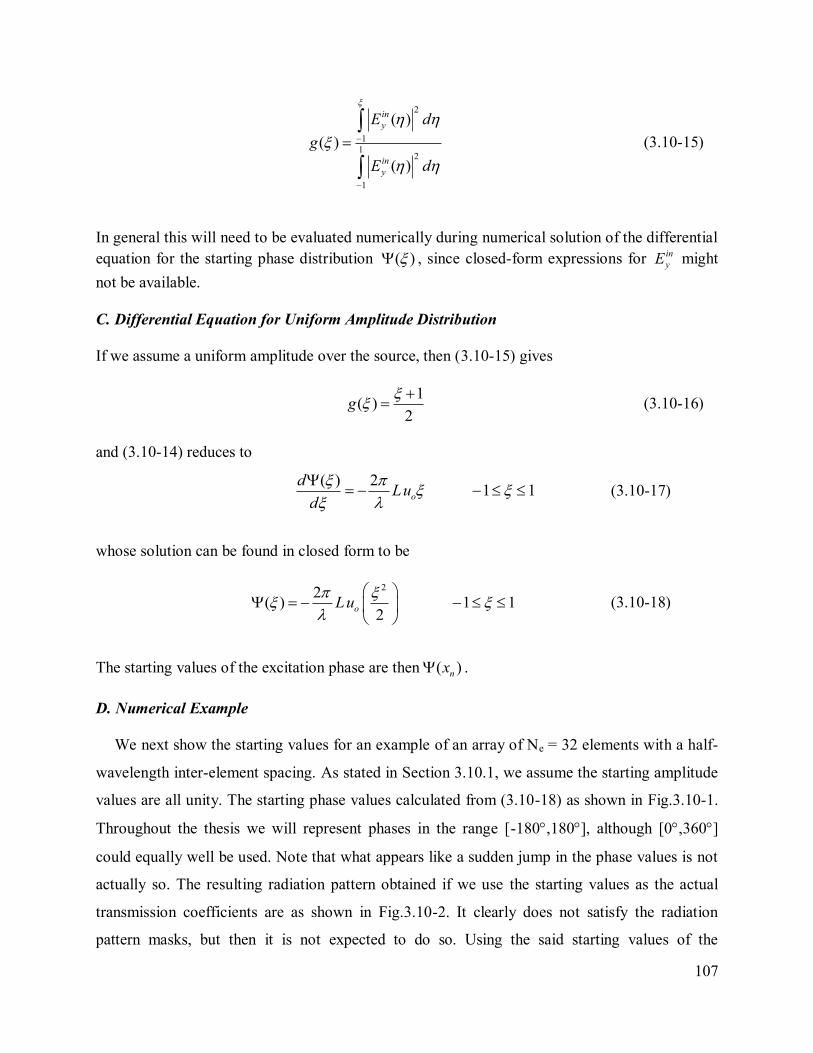
107
2
1
12
1
( )
( )
( )
in
y
in
y
E d
g
E d
(3.10-15)
In general this will need to be evaluated numerically during numerical solution of the differential
equation for the starting phase distribution ( ) , since closed-form expressions for in
yE might
not be available.
C. Differential Equation for Uniform Amplitude Distribution
If we assume a uniform amplitude over the source, then (3.10-15) gives
1( )
2g
(3.10-16)
and (3.10-14) reduces to
( ) 2
1 1o
dLu
d
(3.10-17)
whose solution can be found in closed form to be
22
( ) 1 12
oLu
(3.10-18)
The starting values of the excitation phase are then ( )nx .
D. Numerical Example
We next show the starting values for an example of an array of Ne = 32 elements with a half-
wavelength inter-element spacing. As stated in Section 3.10.1, we assume the starting amplitude
values are all unity. The starting phase values calculated from (3.10-18) as shown in Fig.3.10-1.
Throughout the thesis we will represent phases in the range [-180,180], although [0,360]
could equally well be used. Note that what appears like a sudden jump in the phase values is not
actually so. The resulting radiation pattern obtained if we use the starting values as the actual
transmission coefficients are as shown in Fig.3.10-2. It clearly does not satisfy the radiation
pattern masks, but then it is not expected to do so. Using the said starting values of the
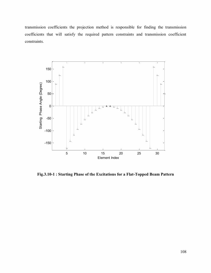
108
transmission coefficients the projection method is responsible for finding the transmission
coefficients that will satisfy the required pattern constraints and transmission coefficient
constraints.
5 10 15 20 25 30
-150
-100
-50
0
50
100
150
Element Index
Sta
rtin
g
Phase A
ngle
(D
egre
s)
Fig.3.10-1 : Starting Phase of the Excitations for a Flat-Topped Beam Pattern
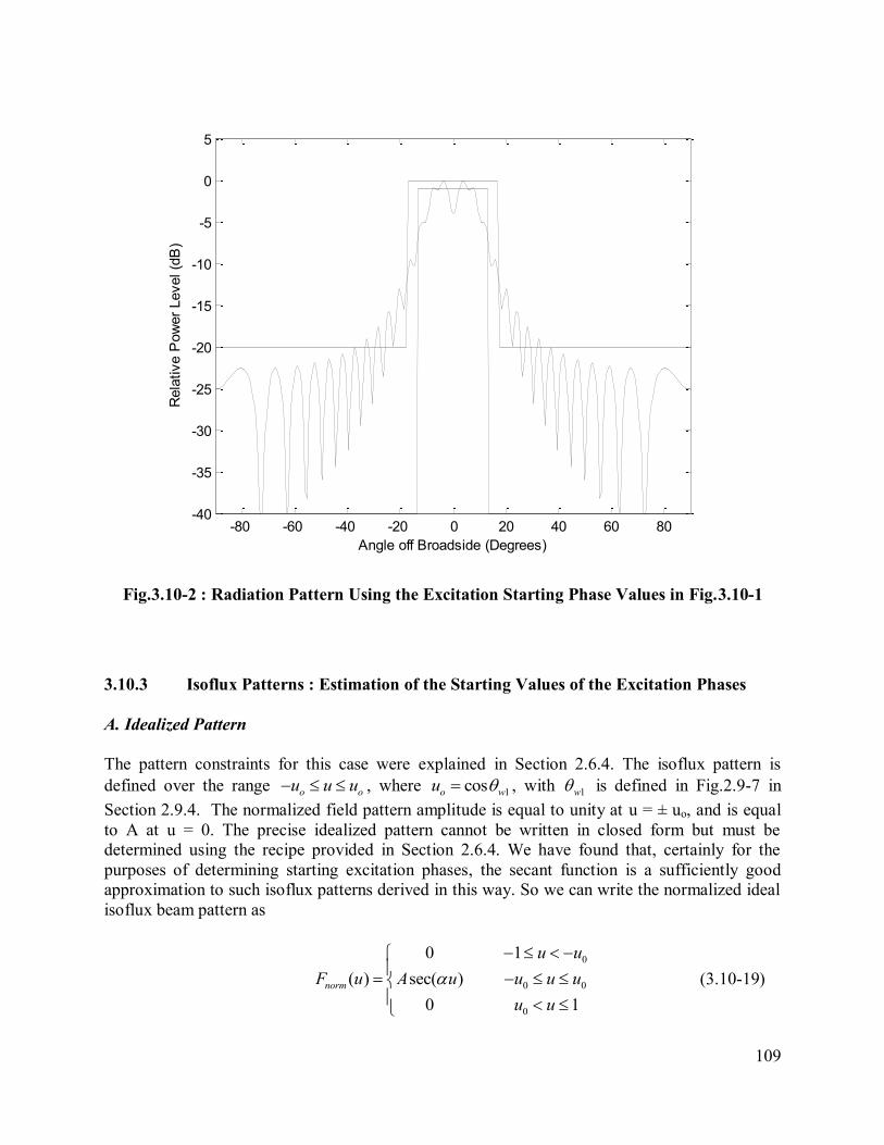
109
-80 -60 -40 -20 0 20 40 60 80-40
-35
-30
-25
-20
-15
-10
-5
0
5
Angle off Broadside (Degrees)
Rela
tive P
ow
er
Level (d
B)
Fig.3.10-2 : Radiation Pattern Using the Excitation Starting Phase Values in Fig.3.10-1
3.10.3 Isoflux Patterns : Estimation of the Starting Values of the Excitation Phases
A. Idealized Pattern
The pattern constraints for this case were explained in Section 2.6.4. The isoflux pattern is
defined over the range o ou u u , where 1coso wu , with 1w is defined in Fig.2.9-7 in
Section 2.9.4. The normalized field pattern amplitude is equal to unity at u = ± uo, and is equal
to A at u = 0. The precise idealized pattern cannot be written in closed form but must be
determined using the recipe provided in Section 2.6.4. We have found that, certainly for the
purposes of determining starting excitation phases, the secant function is a sufficiently good
approximation to such isoflux patterns derived in this way. So we can write the normalized ideal
isoflux beam pattern as
0
0 0
0
0 1
( ) sec( )
0 1
norm
u u
F u A u u u u
u u
(3.10-19)
110
where54
1 1
0 0
1 1sec (1/ ) cos ( )A A
u u (3.10-20)
B. General Case
Using (3.10-19) the expression (3.10-4) becomes
0
0
0
2 2
0
2 02
( ) sec ( )tan( ) tan( )
2 tan( )( ) sec ( )
a
b
a
u u
norm
u u
u u
norm
u u
F d du u
uF d d
(3.10-21)
and so we can write
0
0
tan( ) tan( )( )
2 tan( )
u ug
u
(3.10-22)
and hence
1
0
1( ) tan 2 ( ) 1 tanu g u
(3.10-23)
Use of expression (3.10-6) then results in the differential equation
1
0
( ) 2 1tan 2 ( ) 1 tan 1 1
dL g u
d
(3.10-24)
C. Differential Equation for Uniform Amplitude Distribution
If we assume a uniform amplitude over the source, then ( )g is given by (3.10-22) and (3.10-6)
becomes
1( ) 2 1tan tan( ) 1 1o
dL u
d
(3.10-25)
54 M.R.Spiegel, Mathematical Handbook (McGraw-Hill, 1968) gives 1 1sec cos (1/ ) .
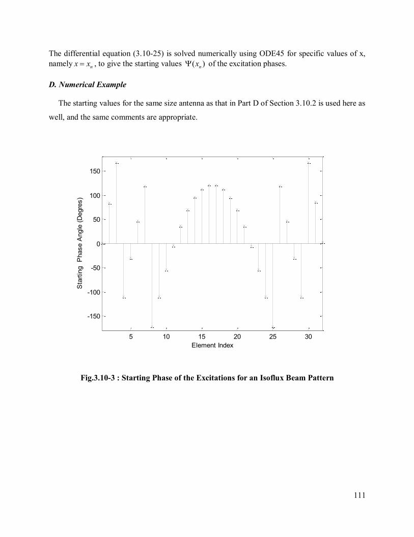
111
The differential equation (3.10-25) is solved numerically using ODE45 for specific values of x,
namelynx x , to give the starting values ( )nx of the excitation phases.
D. Numerical Example
The starting values for the same size antenna as that in Part D of Section 3.10.2 is used here as
well, and the same comments are appropriate.
5 10 15 20 25 30
-150
-100
-50
0
50
100
150
Element Index
Sta
rtin
g
Phase A
ngle
(D
egre
s)
Fig.3.10-3 : Starting Phase of the Excitations for an Isoflux Beam Pattern
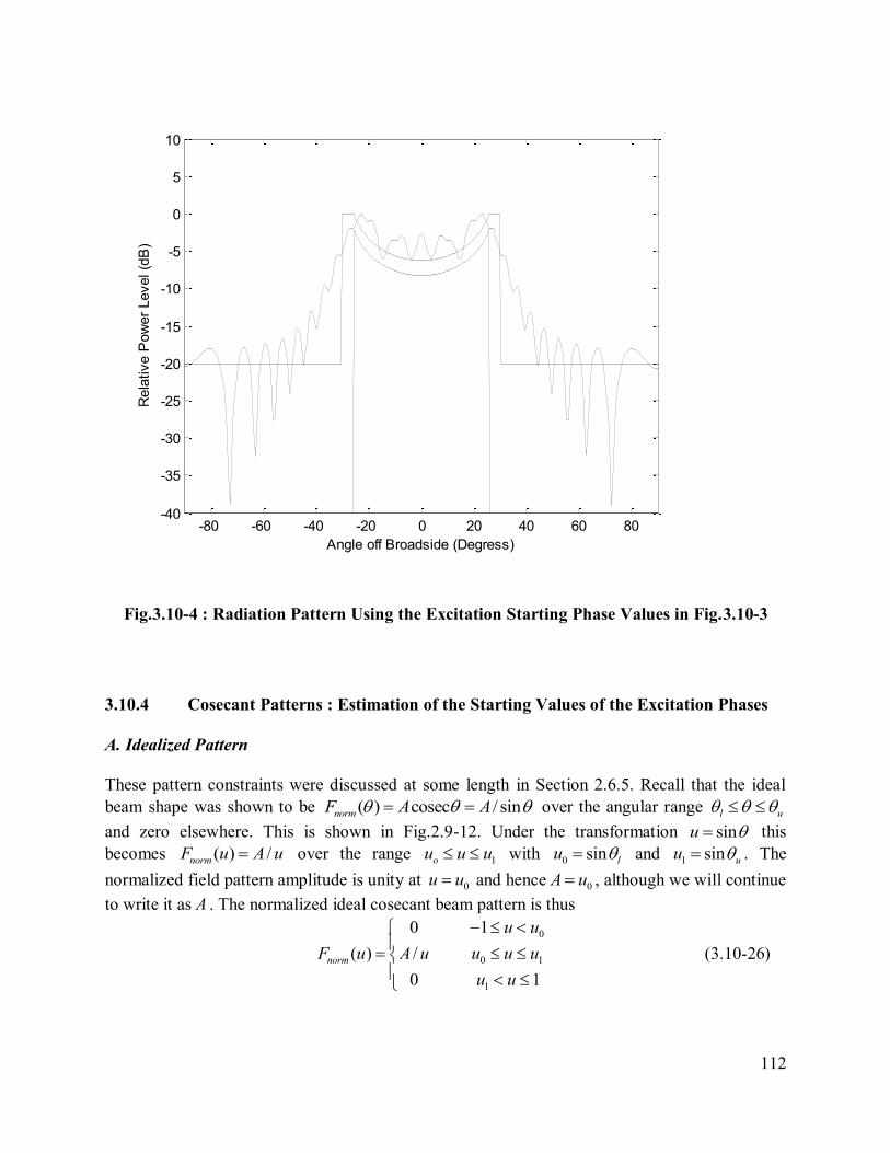
112
-80 -60 -40 -20 0 20 40 60 80-40
-35
-30
-25
-20
-15
-10
-5
0
5
10
Angle off Broadside (Degress)
Rela
tive P
ow
er
Level (d
B)
Fig.3.10-4 : Radiation Pattern Using the Excitation Starting Phase Values in Fig.3.10-3
3.10.4 Cosecant Patterns : Estimation of the Starting Values of the Excitation Phases
A. Idealized Pattern
These pattern constraints were discussed at some length in Section 2.6.5. Recall that the ideal
beam shape was shown to be ( ) cosec / sinnormF A A over the angular range l u
and zero elsewhere. This is shown in Fig.2.9-12. Under the transformation sinu this
becomes ( ) /normF u A u over the range 1ou u u with 0 sin lu and 1 sin uu . The
normalized field pattern amplitude is unity at 0u u and hence 0A u , although we will continue
to write it as A . The normalized ideal cosecant beam pattern is thus
0
0 1
1
0 1
( ) /
0 1
norm
u u
F u A u u u u
u u
(3.10-26)
113
B. General Case
Using (3.10-26) in expression (3.10-4) yields
0
1
0
2 2
0
2 2
0 1
1 1( ) (1/ )
1 1(1/ )( )
a
b
a
u u
norm
u u
u u
norm
uu
F d du u
dF du u
(3.10-27)
and so we can write
0
0 1
1 1
( )1 1
u ug
u u
(3.10-28)
and hence
1
11 1
1 1 1( )
o o
u
gu u u
(3.10-29)
Use of expression (3.10-6) then provides the differential equation
1
( ) 2 11 1
1 1 1( )
o o
dL
dg
u u u
(3.10-30)
C. Differential Equation for Uniform Amplitude Distribution
If we assume a uniform amplitude over the source, then ( )g is given by (3.10-28), and hence
(3.10-30) becomes
1
( ) 2 11 1
1 1 1 1
2o o
dL
d
u u u
(3.10-31)
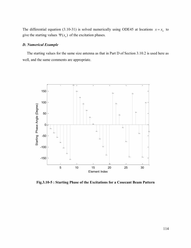
114
The differential equation (3.10-31) is solved numerically using ODE45 at locations nx x to
give the starting values ( )nx of the excitation phases.
D. Numerical Example
The starting values for the same size antenna as that in Part D of Section 3.10.2 is used here as
well, and the same comments are appropriate.
5 10 15 20 25 30
-150
-100
-50
0
50
100
150
Element Index
Sta
rtin
g
Phase A
ngle
(D
egre
s)
Fig.3.10-5 : Starting Phase of the Excitations for a Cosecant Beam Pattern
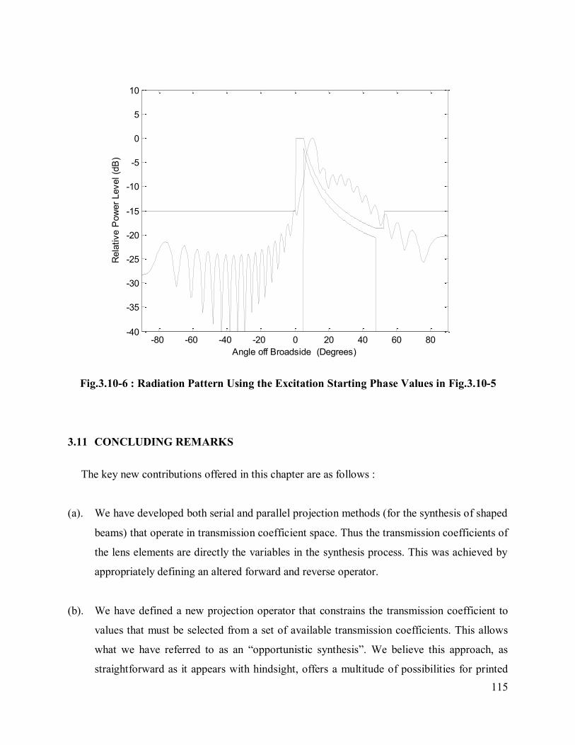
115
-80 -60 -40 -20 0 20 40 60 80-40
-35
-30
-25
-20
-15
-10
-5
0
5
10
Angle off Broadside (Degrees)
Rela
tive P
ow
er
Level (d
B)
Fig.3.10-6 : Radiation Pattern Using the Excitation Starting Phase Values in Fig.3.10-5
3.11 CONCLUDING REMARKS
The key new contributions offered in this chapter are as follows :
(a). We have developed both serial and parallel projection methods (for the synthesis of shaped
beams) that operate in transmission coefficient space. Thus the transmission coefficients of
the lens elements are directly the variables in the synthesis process. This was achieved by
appropriately defining an altered forward and reverse operator.
(b). We have defined a new projection operator that constrains the transmission coefficient to
values that must be selected from a set of available transmission coefficients. This allows
what we have referred to as an “opportunistic synthesis”. We believe this approach, as
straightforward as it appears with hindsight, offers a multitude of possibilities for printed
116
lens antennas / transmitarrays. Transmission coefficient constraints of any kind can be
effectively imposed by simply removing from the database55
.
(c). A very useful approach has been written in structured form for determining the starting
points for a shaped beam synthesis via the projection method. Although the possibility of
using the approach to find starting excitation phase values has been hinted at in at least one
previous publication, details have never actually been given elsewhere. Those provided
here should prove helpful to anyone wishing to use projection synthesis methods56
.
3.12 REFERENCES FOR CHAPTER 3
[1] G. Thiele and W. Stutzman, Antenna Theory & Design (Wiley, 1998)
[2] E. Botha & D. A. McNamara, “Conformal array synthesis using alternating projections, with
maximum likelihood estimation used in one of the projection operators”, Electronics Lett.,
Vol.29, No.20, pp.1733-1734, Sept.1993.
[3] G. Franceschetti, G. Mazzarella & G. Panariello, “Array synthesis with excitation
constraints”, IEE Proc., Vol.135, Pt.H, No.6, pp.400-407, Dec.1988.
[4] O. M.Bucci, G. Franceschetti, G. Mazzarella & G. Panariello, “Intersection approach to
array pattern synthesis”, IEE Proc., Vol.137, Pt.H, No.6, pp.349-357, Dec.1990.
[5] O. M. Bucci, G. Mazzarella & G. Panariello, “Reconfigurable arrays by phase-only
control”, IEEE Trans. Antennas Propagat., Vol.39, No.7, pp.919-925, July 1991.
[6] A. K. Chakraborty, B. N. Das and G. S. Sanyal, “Determination of phase functions for a
desired one-dimensional pattern”, IEEE Trans. Antennas Propagat., Vol. AP-29, No.3,
pp.502-506, May 1981.
[7] A. Chakraborty, B. N. Das and G. S. Sanyal, "Beam shaping using nonlinear phase
distribution in a uniformly spaced array", IEEE Trans. Antennas Propagat., Vol.30,
pp.1031-1034, Sept.1982.
55 They of course do not actually have to be removed. Coding statements can simply prevent the constraint
projection operator from “seeing” them in the transmission coefficient space. In this way the constraints can be
altered without changing the database in anyway. An example is given in Section 4.2.4. 56 This will be further enhanced using the “trap navigation approach” proposed in Section 4.2.4. It is described there
because it was devised while the numerical experiments that are the subject of Chapter 4 were being performed.
117
CHAPTER 4
Application of the Constrained Transmission Coefficient
Synthesis Methods to Shaped Beam Problems
4.1 PRELIMINARY REMARKS
The purpose of this chapter is to implement the formulations developed in Chapter 3. This
involved the creation of the appropriate software, which was composed in a MATLAB [1]
environment. This will be done for the three shaped beam types of interest, in Sections 4.2, 4.3
and 4.4 respectively. It will be conducted systematically, starting with no transmission
coefficient constraints and building up to situations with such constraints. As the transmission
coefficient constraints are tightened the given array will be less able to completely satisfy all the
required pattern constraints. By beginning with no transmission coefficient constraints we can
determine precisely how well the given printed lens can come to the desired beam shape. We
will be able to gauge how much such constraints are responsible for our not exactly achieving the
shaped patterns we want, and by how much we have to relax these pattern specifications. The
penultimate Section 4.5 offers concluding remarks on the chapter, and references are listed in
Section 4.6.
Although a wide range of cases have been executed, unless otherwise stated the examples
whose results are shown apply to the following cylindrical printed lens antennas:
D = 152.4 mm, F/D = 0.5, Ne = 32
D = 191.1 mm, F/D = 0.5, Ne = 40
D = 1112.7 mm, F/D = 0.5, Ne = 24
at an operating frequency of 30 GHz. We need not specify all the pattern mask parameters in
each case (unless some special emphasis is needed) since the masks are included whenever a
pattern is plotted.
In order to apply excitation constraints using the projection synthesis method the pattern
projection operator described in Section 2.7 is applied, irrespective of the particular pattern
mask. The pattern masks for the three canonical shaped beam types of interest in this thesis were
discussed in Section 2.6. The SDE used to track the convergence of the projection synthesis
118
algorithm is that defined in expression (2.7-25). Unless otherwise stated, the serial form of the
projection synthesis method should be assumed.
4.2 FLAT-TOPPED PATTERN SYNTHESIS
4.2.1 Synthesis without Constraints on the Transmission Coefficients
If we use 1nb and 0n o for all elements n = 1 2,3,…..,Ne as the starting values the
projection method does not achieve a successful synthesis. However, if we use starting values
obtained as described in Section 3.10.2, we obtain the radiation pattern result shown in Fig.4.2-1
below. This can be taken as a reference pattern; we should not expect as perfect a satisfaction of
the pattern mask once transmission coefficient constraints are applied. The SDE in Fig.4.2-2
shows that the synthesis converges very rapidly, in fact in less than 20 iterations57
. The required
transmission coefficient amplitudes are depicted in Fig.4.2-3 and Fig.4.2-4, respectively. The
pattern mask58
in this example had an SLR = 20 dB, Srip = 1dB, w1 = 13 and w2 = 17 (so that
w = 4). We have found the synthesis results relatively insensitive to the specific value of the
feed “raised cosine” power between 0 and 3 in the flat-topped beam case, and so have used q =
0.1 throughout.
57 The SDE should always be monitored. Some problems require many more iterations than others. 58 Defined in Fig.2.9-4.
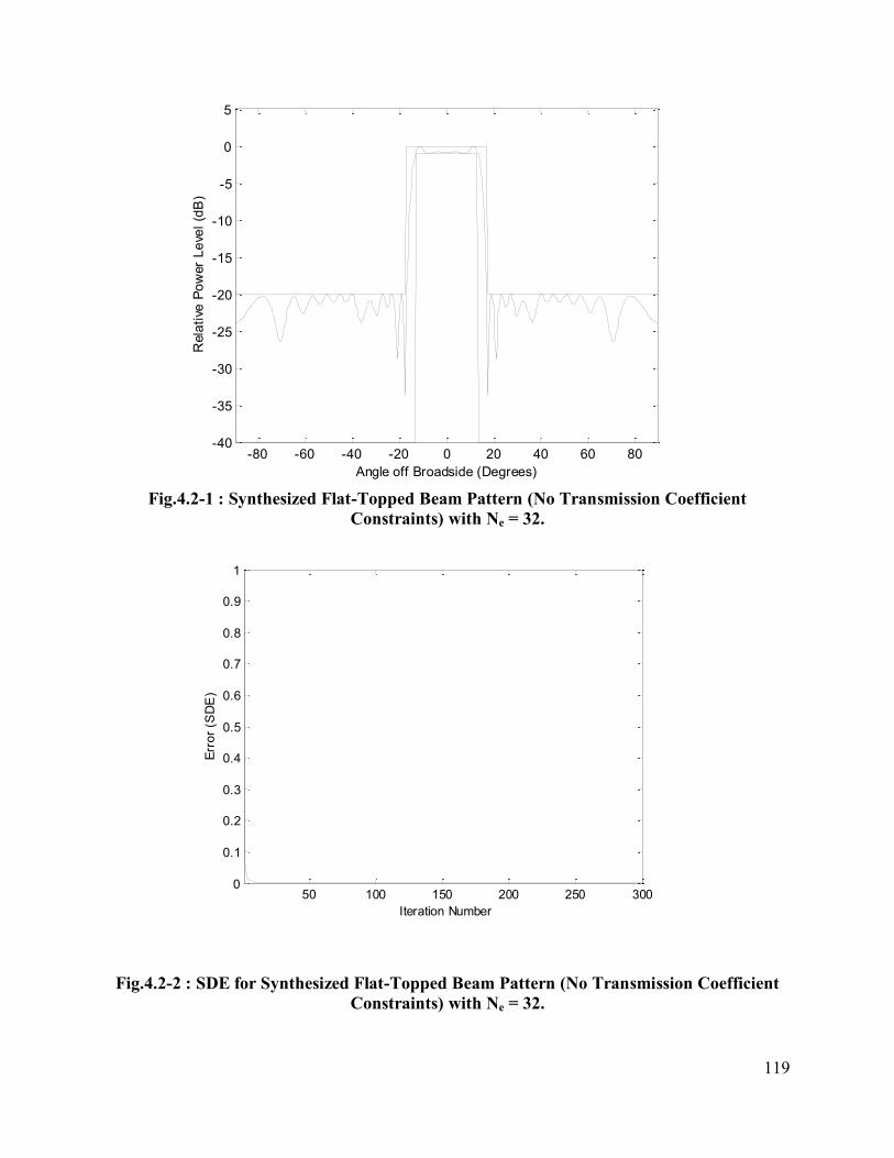
119
Fig.4.2-1 : Synthesized Flat-Topped Beam Pattern (No Transmission Coefficient
Constraints) with Ne = 32.
Fig.4.2-2 : SDE for Synthesized Flat-Topped Beam Pattern (No Transmission Coefficient
Constraints) with Ne = 32.
-80 -60 -40 -20 0 20 40 60 80-40
-35
-30
-25
-20
-15
-10
-5
0
5
Angle off Broadside (Degrees)
Rela
tive
Po
wer
Le
vel
(dB
)
50 100 150 200 250 3000
0.1
0.2
0.3
0.4
0.5
0.6
0.7
0.8
0.9
1
Iteration Number
Err
or
(SD
E)
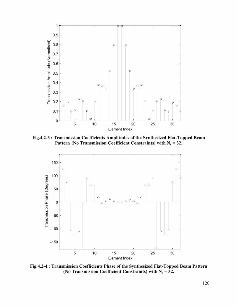
120
Fig.4.2-3 : Transmission Coefficients Amplitudes of the Synthesized Flat-Topped Beam
Pattern (No Transmission Coefficient Constraints) with Ne = 32.
Fig.4.2-4 : Transmission Coefficients Phase of the Synthesized Flat-Topped Beam Pattern
(No Transmission Coefficient Constraints) with Ne = 32.
5 10 15 20 25 300
0.1
0.2
0.3
0.4
0.5
0.6
0.7
0.8
0.9
1
Element Index
Tra
nsm
issi
on
Am
plitu
de
(N
orm
alise
d)
5 10 15 20 25 30
-150
-100
-50
0
50
100
150
Element Index
Tra
nsm
issi
on
Ph
ase
(D
eg
ree
s)
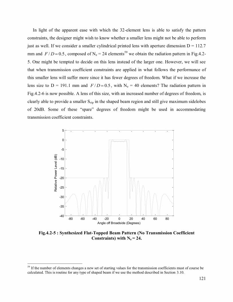
121
In light of the apparent ease with which the 32-element lens is able to satisfy the pattern
constraints, the designer might wish to know whether a smaller lens might not be able to perform
just as well. If we consider a smaller cylindrical printed lens with aperture dimension D = 112.7
mm and / 0.5F D , composed of Ne = 24 elements59
we obtain the radiation pattern in Fig.4.2-
5. One might be tempted to decide on this lens instead of the larger one. However, we will see
that when transmission coefficient constraints are applied in what follows the performance of
this smaller lens will suffer more since it has fewer degrees of freedom. What if we increase the
lens size to D = 191.1 mm and / 0.5F D , with Ne = 40 elements? The radiation pattern in
Fig.4.2-6 is now possible. A lens of this size, with an increased number of degrees of freedom, is
clearly able to provide a smaller Srip in the shaped beam region and still give maximum sidelobes
of 20dB. Some of these “spare” degrees of freedom might be used in accommodating
transmission coefficient constraints.
-80 -60 -40 -20 0 20 40 60 80-40
-35
-30
-25
-20
-15
-10
-5
0
5
Angle off Broadside (Degrees)
Rela
tive P
ow
er
Level (d
B)
Fig.4.2-5 : Synthesized Flat-Topped Beam Pattern (No Transmission Coefficient
Constraints) with Ne = 24.
59 If the number of elements changes a new set of starting values for the transmission coefficients must of course be
calculated. This is routine for any type of shaped beam if we use the method described in Section 3.10.
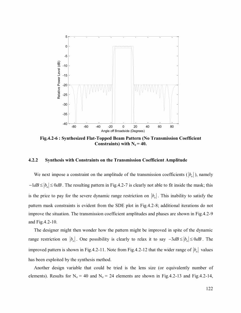
122
-80 -60 -40 -20 0 20 40 60 80-40
-35
-30
-25
-20
-15
-10
-5
0
5
Angle off Broadside (Degrees)
Rela
tive P
ow
er
Level (d
B)
Fig.4.2-6 : Synthesized Flat-Topped Beam Pattern (No Transmission Coefficient
Constraints) with Ne = 40.
4.2.2 Synthesis with Constraints on the Transmission Coefficient Amplitude
We next impose a constraint on the amplitude of the transmission coefficients ( nb ), namely
1 0ndB b dB . The resulting pattern in Fig.4.2-7 is clearly not able to fit inside the mask; this
is the price to pay for the severe dynamic range restriction on nb . This inability to satisfy the
pattern mask constraints is evident from the SDE plot in Fig.4.2-8; additional iterations do not
improve the situation. The transmission coefficient amplitudes and phases are shown in Fig.4.2-9
and Fig.4.2-10.
The designer might then wonder how the pattern might be improved in spite of the dynamic
range restriction on nb . One possibility is clearly to relax it to say 3 0ndB b dB . The
improved pattern is shown in Fig.4.2-11. Note from Fig.4.2-12 that the wider range of nb values
has been exploited by the synthesis method.
Another design variable that could be tried is the lens size (or equivalently number of
elements). Results for Ne = 40 and Ne = 24 elements are shown in Fig.4.2-13 and Fig.4.2-14,
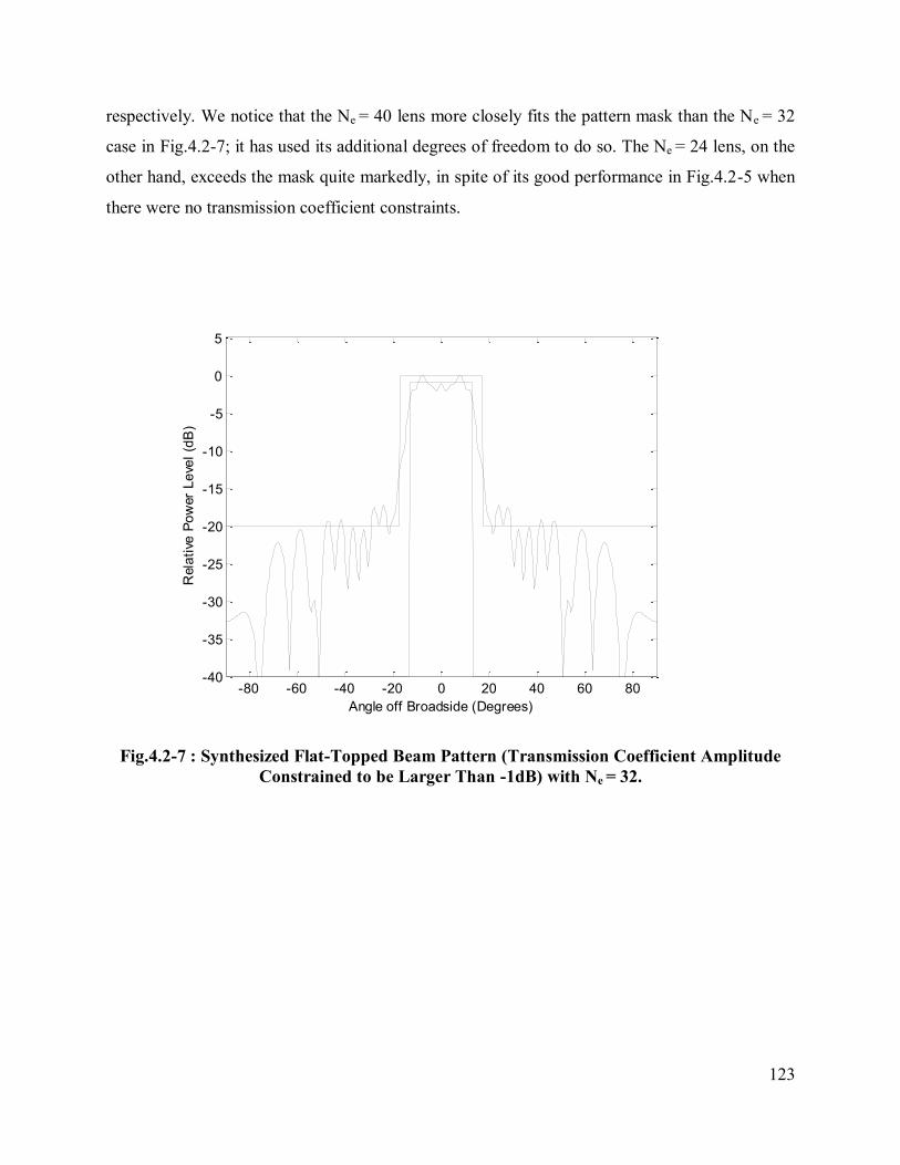
123
respectively. We notice that the Ne = 40 lens more closely fits the pattern mask than the Ne = 32
case in Fig.4.2-7; it has used its additional degrees of freedom to do so. The Ne = 24 lens, on the
other hand, exceeds the mask quite markedly, in spite of its good performance in Fig.4.2-5 when
there were no transmission coefficient constraints.
Fig.4.2-7 : Synthesized Flat-Topped Beam Pattern (Transmission Coefficient Amplitude
Constrained to be Larger Than -1dB) with Ne = 32.
-80 -60 -40 -20 0 20 40 60 80-40
-35
-30
-25
-20
-15
-10
-5
0
5
Angle off Broadside (Degrees)
Rela
tive
Po
wer
Le
vel
(dB
)
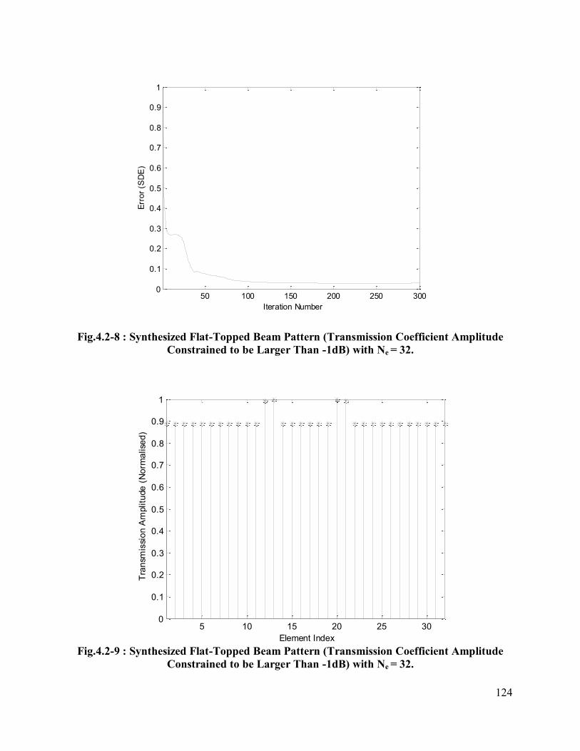
124
Fig.4.2-8 : Synthesized Flat-Topped Beam Pattern (Transmission Coefficient Amplitude
Constrained to be Larger Than -1dB) with Ne = 32.
Fig.4.2-9 : Synthesized Flat-Topped Beam Pattern (Transmission Coefficient Amplitude
Constrained to be Larger Than -1dB) with Ne = 32.
50 100 150 200 250 3000
0.1
0.2
0.3
0.4
0.5
0.6
0.7
0.8
0.9
1
Iteration Number
Err
or
(SD
E)
5 10 15 20 25 300
0.1
0.2
0.3
0.4
0.5
0.6
0.7
0.8
0.9
1
Element Index
Tra
nsm
issi
on
Am
plitu
de
(N
orm
alise
d)
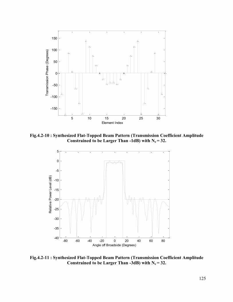
125
Fig.4.2-10 : Synthesized Flat-Topped Beam Pattern (Transmission Coefficient Amplitude
Constrained to be Larger Than -1dB) with Ne = 32.
-80 -60 -40 -20 0 20 40 60 80-40
-35
-30
-25
-20
-15
-10
-5
0
5
Angle off Broadside (Degrees)
Rela
tive P
ow
er
Level (d
B)
Fig.4.2-11 : Synthesized Flat-Topped Beam Pattern (Transmission Coefficient Amplitude
Constrained to be Larger Than -3dB) with Ne = 32.
5 10 15 20 25 30
-150
-100
-50
0
50
100
150
Element Index
Tra
nsm
issi
on
Ph
ase
(D
eg
ree
s)
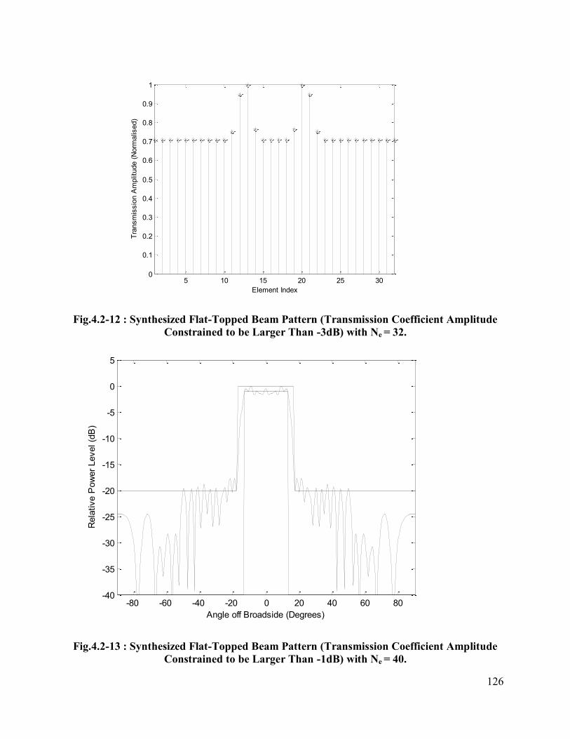
126
5 10 15 20 25 300
0.1
0.2
0.3
0.4
0.5
0.6
0.7
0.8
0.9
1
Element Index
Tra
nsm
issio
n A
mplit
ude (
Norm
alis
ed)
Fig.4.2-12 : Synthesized Flat-Topped Beam Pattern (Transmission Coefficient Amplitude
Constrained to be Larger Than -3dB) with Ne = 32.
-80 -60 -40 -20 0 20 40 60 80-40
-35
-30
-25
-20
-15
-10
-5
0
5
Angle off Broadside (Degrees)
Rela
tive P
ow
er
Level (d
B)
Fig.4.2-13 : Synthesized Flat-Topped Beam Pattern (Transmission Coefficient Amplitude
Constrained to be Larger Than -1dB) with Ne = 40.
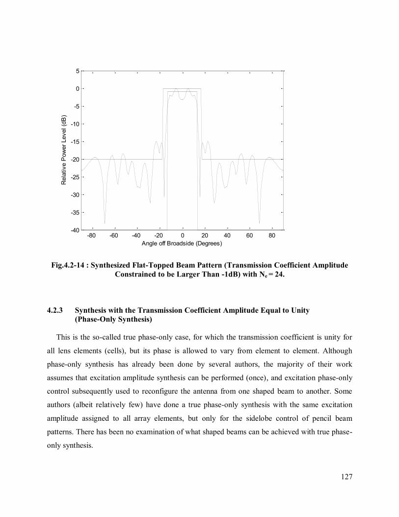
127
-80 -60 -40 -20 0 20 40 60 80-40
-35
-30
-25
-20
-15
-10
-5
0
5
Angle off Broadside (Degrees)
Rela
tive P
ow
er
Level (d
B)
Fig.4.2-14 : Synthesized Flat-Topped Beam Pattern (Transmission Coefficient Amplitude
Constrained to be Larger Than -1dB) with Ne = 24.
4.2.3 Synthesis with the Transmission Coefficient Amplitude Equal to Unity
(Phase-Only Synthesis)
This is the so-called true phase-only case, for which the transmission coefficient is unity for
all lens elements (cells), but its phase is allowed to vary from element to element. Although
phase-only synthesis has already been done by several authors, the majority of their work
assumes that excitation amplitude synthesis can be performed (once), and excitation phase-only
control subsequently used to reconfigure the antenna from one shaped beam to another. Some
authors (albeit relatively few) have done a true phase-only synthesis with the same excitation
amplitude assigned to all array elements, but only for the sidelobe control of pencil beam
patterns. There has been no examination of what shaped beams can be achieved with true phase-
only synthesis.
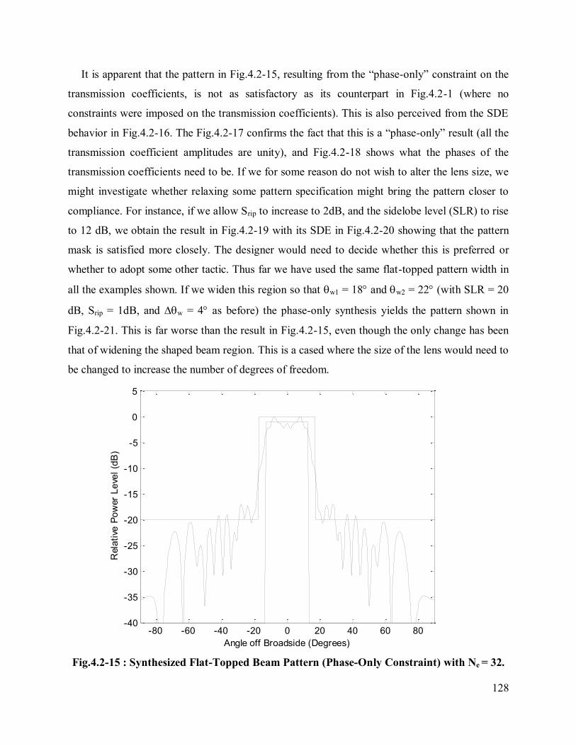
128
It is apparent that the pattern in Fig.4.2-15, resulting from the “phase-only” constraint on the
transmission coefficients, is not as satisfactory as its counterpart in Fig.4.2-1 (where no
constraints were imposed on the transmission coefficients). This is also perceived from the SDE
behavior in Fig.4.2-16. The Fig.4.2-17 confirms the fact that this is a “phase-only” result (all the
transmission coefficient amplitudes are unity), and Fig.4.2-18 shows what the phases of the
transmission coefficients need to be. If we for some reason do not wish to alter the lens size, we
might investigate whether relaxing some pattern specification might bring the pattern closer to
compliance. For instance, if we allow Srip to increase to 2dB, and the sidelobe level (SLR) to rise
to 12 dB, we obtain the result in Fig.4.2-19 with its SDE in Fig.4.2-20 showing that the pattern
mask is satisfied more closely. The designer would need to decide whether this is preferred or
whether to adopt some other tactic. Thus far we have used the same flat-topped pattern width in
all the examples shown. If we widen this region so that w1 = 18 and w2 = 22 (with SLR = 20
dB, Srip = 1dB, and w = 4 as before) the phase-only synthesis yields the pattern shown in
Fig.4.2-21. This is far worse than the result in Fig.4.2-15, even though the only change has been
that of widening the shaped beam region. This is a cased where the size of the lens would need to
be changed to increase the number of degrees of freedom.
Fig.4.2-15 : Synthesized Flat-Topped Beam Pattern (Phase-Only Constraint) with Ne = 32.
-80 -60 -40 -20 0 20 40 60 80-40
-35
-30
-25
-20
-15
-10
-5
0
5
Angle off Broadside (Degrees)
Rela
tive
Po
wer
Le
vel
(dB
)
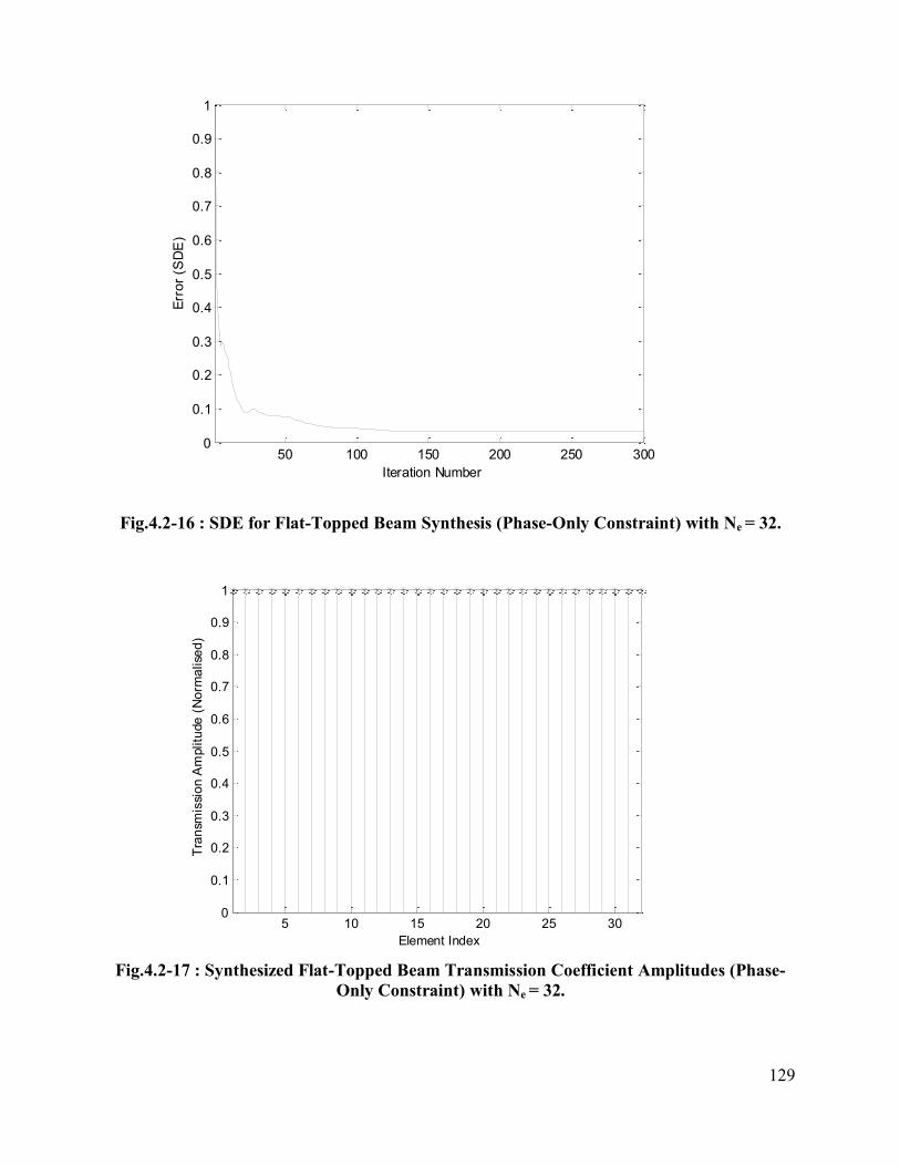
129
Fig.4.2-16 : SDE for Flat-Topped Beam Synthesis (Phase-Only Constraint) with Ne = 32.
Fig.4.2-17 : Synthesized Flat-Topped Beam Transmission Coefficient Amplitudes (Phase-
Only Constraint) with Ne = 32.
5 10 15 20 25 300
0.1
0.2
0.3
0.4
0.5
0.6
0.7
0.8
0.9
1
Element Index
Tra
nsm
issi
on
Am
plitu
de
(N
orm
alise
d)
50 100 150 200 250 3000
0.1
0.2
0.3
0.4
0.5
0.6
0.7
0.8
0.9
1
Iteration Number
Err
or
(SD
E)
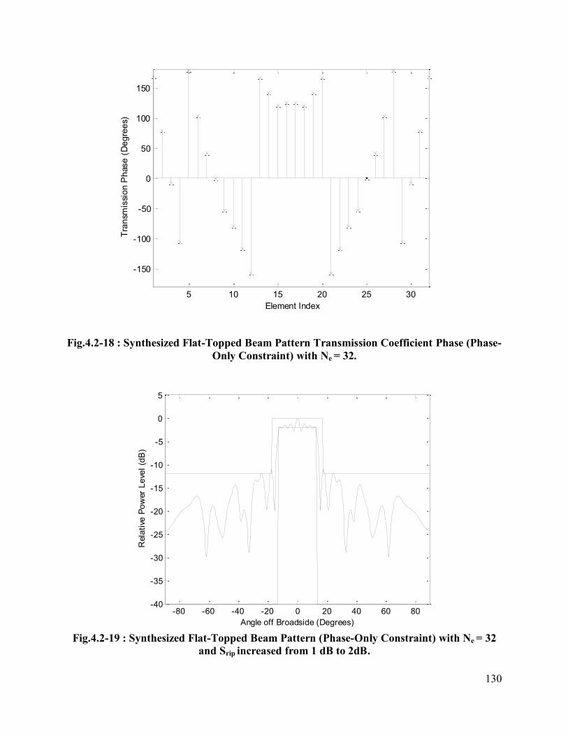
130
Fig.4.2-18 : Synthesized Flat-Topped Beam Pattern Transmission Coefficient Phase (Phase-
Only Constraint) with Ne = 32.
Fig.4.2-19 : Synthesized Flat-Topped Beam Pattern (Phase-Only Constraint) with Ne = 32
and Srip increased from 1 dB to 2dB.
5 10 15 20 25 30
-150
-100
-50
0
50
100
150
Element Index
Tra
nsm
issi
on
Ph
ase
(D
eg
ree
s)
-80 -60 -40 -20 0 20 40 60 80-40
-35
-30
-25
-20
-15
-10
-5
0
5
Angle off Broadside (Degrees)
Rela
tive
Po
wer
Le
vel
(dB
)
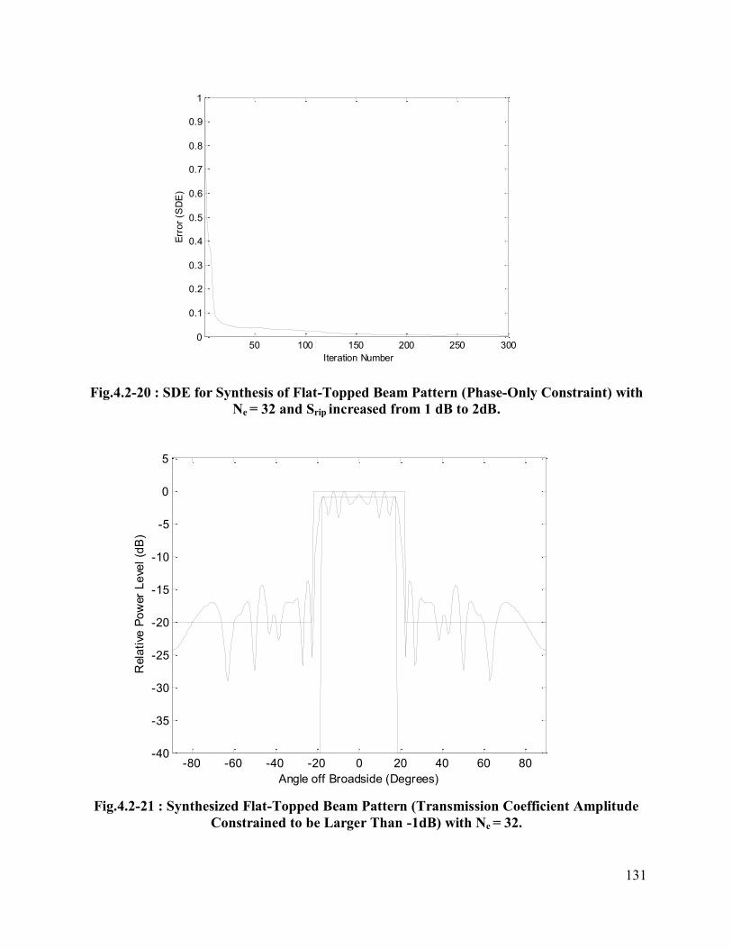
131
Fig.4.2-20 : SDE for Synthesis of Flat-Topped Beam Pattern (Phase-Only Constraint) with
Ne = 32 and Srip increased from 1 dB to 2dB.
Fig.4.2-21 : Synthesized Flat-Topped Beam Pattern (Transmission Coefficient Amplitude
Constrained to be Larger Than -1dB) with Ne = 32.
50 100 150 200 250 3000
0.1
0.2
0.3
0.4
0.5
0.6
0.7
0.8
0.9
1
Iteration Number
Err
or
(SD
E)
-80 -60 -40 -20 0 20 40 60 80-40
-35
-30
-25
-20
-15
-10
-5
0
5
Angle off Broadside (Degrees)
Rela
tive
Po
wer
Le
vel
(dB
)
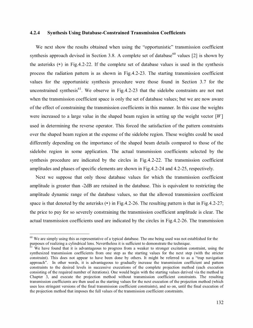
132
4.2.4 Synthesis Using Database-Constrained Transmission Coefficients
We next show the results obtained when using the “opportunistic” transmission coefficient
synthesis approach devised in Section 3.8. A complete set of database60
values [2] is shown by
the asterisks () in Fig.4.2-22. If the complete set of database values is used in the synthesis
process the radiation pattern is as shown in Fig.4.2-23. The starting transmission coefficient
values for the opportunistic synthesis procedure were those found in Section 3.7 for the
unconstrained synthesis61
. We observe in Fig.4.2-23 that the sidelobe constraints are not met
when the transmission coefficient space is only the set of database values; but we are now aware
of the effect of constraining the transmission coefficients in this manner. In this case the weights
were increased to a large value in the shaped beam region in setting up the weight vector [ ]W
used in determining the reverse operator. This forced the satisfaction of the pattern constraints
over the shaped beam region at the expense of the sidelobe region. These weights could be used
differently depending on the importance of the shaped beam details compared to those of the
sidelobe region in some application. The actual transmission coefficients selected by the
synthesis procedure are indicated by the circles in Fig.4.2-22. The transmission coefficient
amplitudes and phases of specific elements are shown in Fig.4.2-24 and 4.2-25, respectively.
Next we suppose that only those database values for which the transmission coefficient
amplitude is greater than -2dB are retained in the database. This is equivalent to restricting the
amplitude dynamic range of the database values, so that the allowed transmission coefficient
space is that denoted by the asterisks () in Fig.4.2-26. The resulting pattern is that in Fig.4.2-27;
the price to pay for so severely constraining the transmission coefficient amplitude is clear. The
actual transmission coefficients used are indicated by the circles in Fig.4.2-26. The transmission
60 We are simply using this as representative of a typical database. The one being used was not established for the
purposes of realizing a cylindrical lens. Nevertheless it is sufficient to demonstrate the technique. 61 We have found that it is advantageous to progress from a weaker to stronger excitation constraint, using the
synthesized transmission coefficients from one step as the starting values for the next step (with the stricter
constraint). This does not appear to have been done by others. It might be referred to as a “trap navigation
approach”. In other words, it is advantageous to gradually increase the transmission coefficient and pattern
constraints to the desired levels in successive executions of the complete projection method (each execution
consisting of the required number of iterations). One would begin with the starting values derived via the method in Chapter 3, and execute the projection method without transmission coefficient constraints. The resulting
transmission coefficients are then used as the starting values for the next execution of the projection method (which
uses less stringent versions of the final transmission coefficient constraints), and so on, until the final execution of
the projection method that imposes the full values of the transmission coefficient constraints.
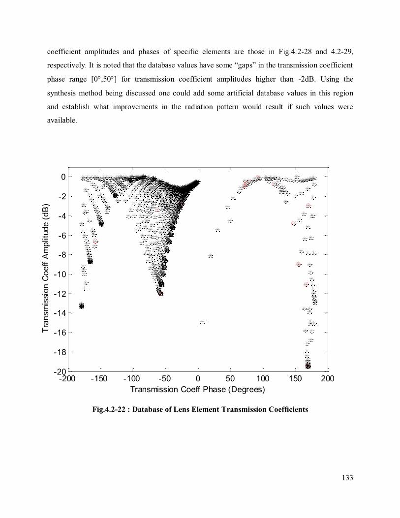
133
coefficient amplitudes and phases of specific elements are those in Fig.4.2-28 and 4.2-29,
respectively. It is noted that the database values have some “gaps” in the transmission coefficient
phase range [0,50] for transmission coefficient amplitudes higher than -2dB. Using the
synthesis method being discussed one could add some artificial database values in this region
and establish what improvements in the radiation pattern would result if such values were
available.
Fig.4.2-22 : Database of Lens Element Transmission Coefficients
-200 -150 -100 -50 0 50 100 150 200-20
-18
-16
-14
-12
-10
-8
-6
-4
-2
0
Transmission Coeff Phase (Degrees)
Tra
nsm
issi
on
Co
eff
Am
plitu
de
(d
B)
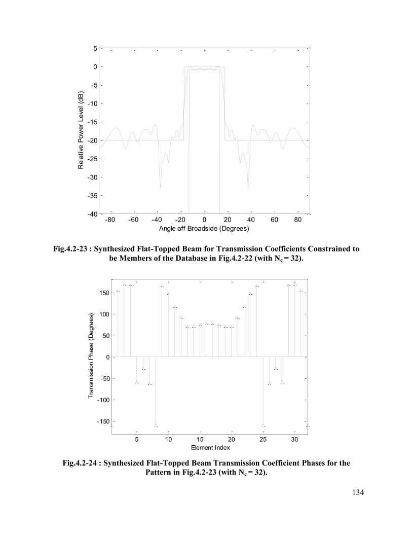
134
Fig.4.2-23 : Synthesized Flat-Topped Beam for Transmission Coefficients Constrained to
be Members of the Database in Fig.4.2-22 (with Ne = 32).
Fig.4.2-24 : Synthesized Flat-Topped Beam Transmission Coefficient Phases for the
Pattern in Fig.4.2-23 (with Ne = 32).
-80 -60 -40 -20 0 20 40 60 80-40
-35
-30
-25
-20
-15
-10
-5
0
5
Angle off Broadside (Degrees)
Rela
tive
Po
wer
Le
vel
(dB
)
5 10 15 20 25 30
-150
-100
-50
0
50
100
150
Element Index
Tra
nsm
issi
on
Ph
ase
(D
eg
ree
s)
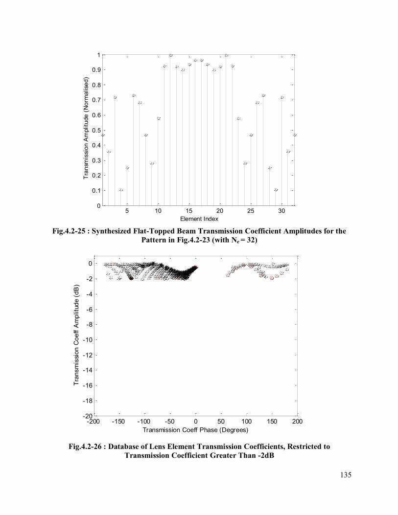
135
Fig.4.2-25 : Synthesized Flat-Topped Beam Transmission Coefficient Amplitudes for the
Pattern in Fig.4.2-23 (with Ne = 32)
Fig.4.2-26 : Database of Lens Element Transmission Coefficients, Restricted to
Transmission Coefficient Greater Than -2dB
5 10 15 20 25 300
0.1
0.2
0.3
0.4
0.5
0.6
0.7
0.8
0.9
1
Element Index
Tra
nsm
issi
on
Am
plitu
de
(N
orm
alise
d)
-200 -150 -100 -50 0 50 100 150 200-20
-18
-16
-14
-12
-10
-8
-6
-4
-2
0
Transmission Coeff Phase (Degrees)
Tra
nsm
issi
on
Co
eff
Am
plitu
de
(d
B)
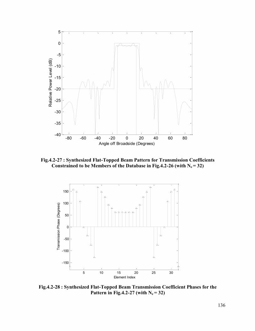
136
Fig.4.2-27 : Synthesized Flat-Topped Beam Pattern for Transmission Coefficients
Constrained to be Members of the Database in Fig.4.2-26 (with Ne = 32)
Fig.4.2-28 : Synthesized Flat-Topped Beam Transmission Coefficient Phases for the
Pattern in Fig.4.2-27 (with Ne = 32)
-80 -60 -40 -20 0 20 40 60 80-40
-35
-30
-25
-20
-15
-10
-5
0
5
Angle off Broadside (Degrees)
Rela
tive
Po
wer
Le
vel
(dB
)
5 10 15 20 25 30
-150
-100
-50
0
50
100
150
Element Index
Tra
nsm
issi
on
Ph
ase
(D
eg
ree
s)
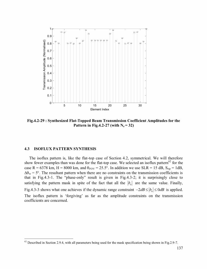
137
Fig.4.2-29 : Synthesized Flat-Topped Beam Transmission Coefficient Amplitudes for the
Pattern in Fig.4.2-27 (with Ne = 32)
4.3 ISOFLUX PATTERN SYNTHESIS
The isoflux pattern is, like the flat-top case of Section 4.2, symmetrical. We will therefore
show fewer examples than was done for the flat-top case. We selected an isoflux pattern62
for the
case R = 6378 km, H = 8000 km, and FOV = 25.5. In addition we use SLR = 15 dB, Srip = 1dB,
w = 5. The resultant pattern when there are no constraints on the transmission coefficients is
that in Fig.4.3-1. The “phase-only” result is given in Fig.4.3-2; it is surprisingly close to
satisfying the pattern mask in spite of the fact that all the nb are the same value. Finally,
Fig.4.3-3 shows what one achieves if the dynamic range constraint 2 0ndB b dB is applied.
The isoflux pattern is ‘forgiving’ as far as the amplitude constraints on the transmission
coefficients are concerned.
62 Described in Section 2.9.4, with all parameters being used for the mask specification being shown in Fig.2.9-7.
5 10 15 20 25 300
0.1
0.2
0.3
0.4
0.5
0.6
0.7
0.8
0.9
1
Element Index
Tra
nsm
issi
on
Am
plitu
de
(N
orm
alise
d)
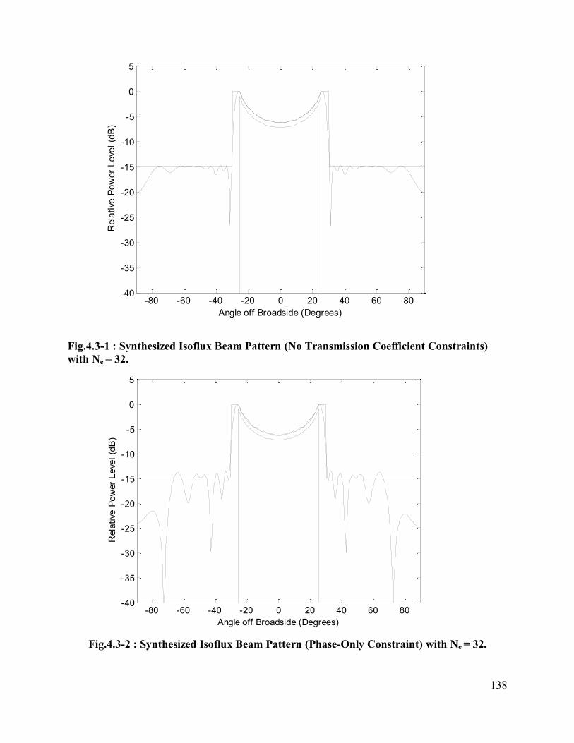
138
Fig.4.3-1 : Synthesized Isoflux Beam Pattern (No Transmission Coefficient Constraints)
with Ne = 32.
Fig.4.3-2 : Synthesized Isoflux Beam Pattern (Phase-Only Constraint) with Ne = 32.
-80 -60 -40 -20 0 20 40 60 80-40
-35
-30
-25
-20
-15
-10
-5
0
5
Angle off Broadside (Degrees)
Rela
tive
Po
wer
Le
vel
(dB
)
-80 -60 -40 -20 0 20 40 60 80-40
-35
-30
-25
-20
-15
-10
-5
0
5
Angle off Broadside (Degrees)
Rela
tive
Po
wer
Le
vel
(dB
)
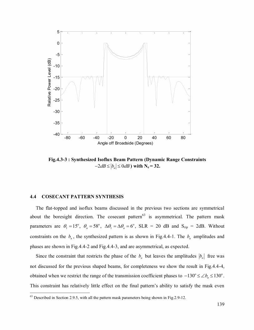
139
Fig.4.3-3 : Synthesized Isoflux Beam Pattern (Dynamic Range Constraints
2 0ndB b dB ) with Ne = 32.
4.4 COSECANT PATTERN SYNTHESIS
The flat-topped and isoflux beams discussed in the previous two sections are symmetrical
about the boresight direction. The cosecant pattern63
is asymmetrical. The pattern mask
parameters are 15 o
l , 58u o , 6u o
l , SLR = 20 dB and Srip = 2dB. Without
constraints on the nb , the synthesized pattern is as shown in Fig.4.4-1. The nb amplitudes and
phases are shown in Fig.4.4-2 and Fig.4.4-3, and are asymmetrical, as expected.
Since the constraint that restricts the phase of the nb but leaves the amplitudes nb free was
not discussed for the previous shaped beams, for completeness we show the result in Fig.4.4-4,
obtained when we restrict the range of the transmission coefficient phases to 130 130nb o o.
This constraint has relatively little effect on the final pattern’s ability to satisfy the mask even
63 Described in Section 2.9.5, with all the pattern mask parameters being shown in Fig.2.9-12.
-80 -60 -40 -20 0 20 40 60 80-40
-35
-30
-25
-20
-15
-10
-5
0
5
Angle off Broadside (Degrees)
Rela
tive
Po
wer
Le
vel
(dB
)
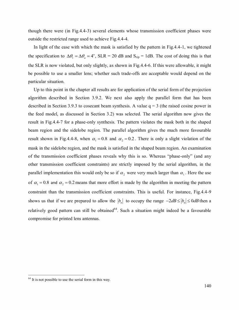
140
though there were (in Fig.4.4-3) several elements whose transmission coefficient phases were
outside the restricted range used to achieve Fig.4.4-4.
In light of the ease with which the mask is satisfied by the pattern in Fig.4.4-1, we tightened
the specification to 4u o
l, SLR = 20 dB and Srip = 1dB. The cost of doing this is that
the SLR is now violated, but only slightly, as shown in Fig.4.4-6. If this were allowable, it might
be possible to use a smaller lens; whether such trade-offs are acceptable would depend on the
particular situation.
Up to this point in the chapter all results are for application of the serial form of the projection
algorithm described in Section 3.9.2. We next also apply the parallel form that has been
described in Section 3.9.3 to cosecant beam synthesis. A value q = 3 (the raised cosine power in
the feed model, as discussed in Section 3.2) was selected. The serial algorithm now gives the
result in Fig.4.4-7 for a phase-only synthesis. The pattern violates the mask both in the shaped
beam region and the sidelobe region. The parallel algorithm gives the much more favourable
result shown in Fig.4.4-8, when 1 0.8 and 2 0.2 . There is only a slight violation of the
mask in the sidelobe region, and the mask is satisfied in the shaped beam region. An examination
of the transmission coefficient phases reveals why this is so. Whereas “phase-only” (and any
other transmission coefficient constraints) are strictly imposed by the serial algorithm, in the
parallel implementation this would only be so if 2 were very much larger than 1 . Here the use
of 1 0.8 and 2 0.2 means that more effort is made by the algorithm in meeting the pattern
constraint than the transmission coefficient constraints. This is useful. For instance, Fig.4.4-9
shows us that if we are prepared to allow the nb to occupy the range 2 0ndB b dB then a
relatively good pattern can still be obtained64
. Such a situation might indeed be a favourable
compromise for printed lens antennas.
64 It is not possible to use the serial form in this way.
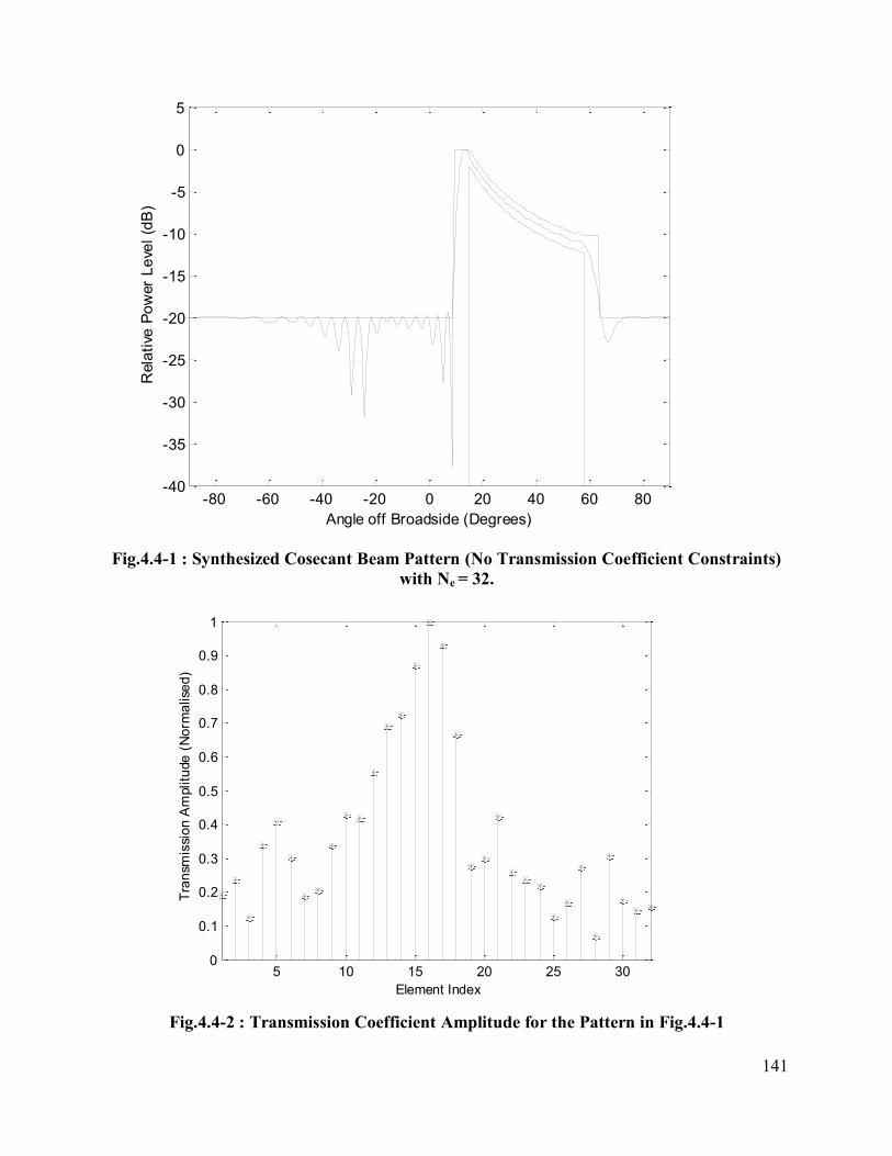
141
Fig.4.4-1 : Synthesized Cosecant Beam Pattern (No Transmission Coefficient Constraints)
with Ne = 32.
Fig.4.4-2 : Transmission Coefficient Amplitude for the Pattern in Fig.4.4-1
-80 -60 -40 -20 0 20 40 60 80-40
-35
-30
-25
-20
-15
-10
-5
0
5
Angle off Broadside (Degrees)
Rela
tive
Po
wer
Le
vel
(dB
)
5 10 15 20 25 300
0.1
0.2
0.3
0.4
0.5
0.6
0.7
0.8
0.9
1
Element Index
Tra
nsm
issi
on
Am
plitu
de
(N
orm
alise
d)
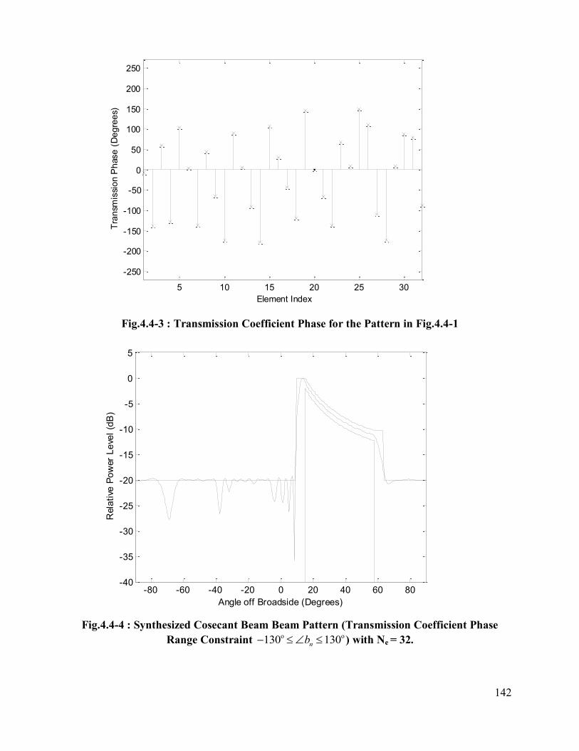
142
Fig.4.4-3 : Transmission Coefficient Phase for the Pattern in Fig.4.4-1
Fig.4.4-4 : Synthesized Cosecant Beam Beam Pattern (Transmission Coefficient Phase
Range Constraint 130 130nb o o) with Ne = 32.
5 10 15 20 25 30
-250
-200
-150
-100
-50
0
50
100
150
200
250
Element Index
Tra
nsm
issi
on
Ph
ase
(D
eg
ree
s)
-80 -60 -40 -20 0 20 40 60 80-40
-35
-30
-25
-20
-15
-10
-5
0
5
Angle off Broadside (Degrees)
Rela
tive
Po
wer
Le
vel
(dB
)
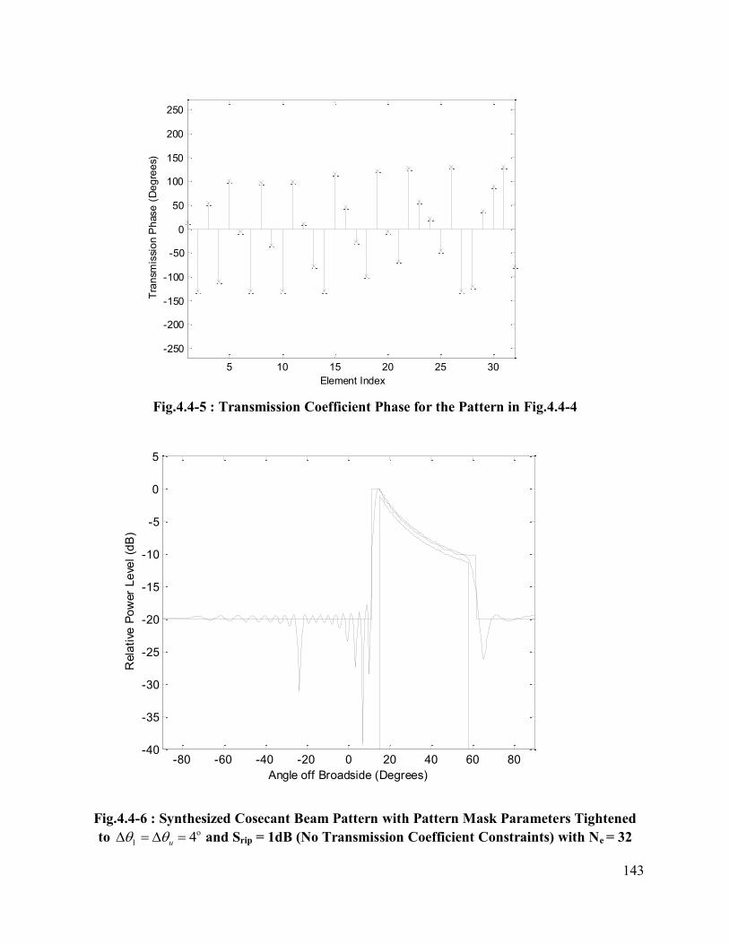
143
Fig.4.4-5 : Transmission Coefficient Phase for the Pattern in Fig.4.4-4
Fig.4.4-6 : Synthesized Cosecant Beam Pattern with Pattern Mask Parameters Tightened
to 4u o
l and Srip = 1dB (No Transmission Coefficient Constraints) with Ne = 32
5 10 15 20 25 30
-250
-200
-150
-100
-50
0
50
100
150
200
250
Element Index
Tra
nsm
issi
on
Ph
ase
(D
eg
ree
s)
-80 -60 -40 -20 0 20 40 60 80-40
-35
-30
-25
-20
-15
-10
-5
0
5
Angle off Broadside (Degrees)
Rela
tive
Po
wer
Le
vel
(dB
)
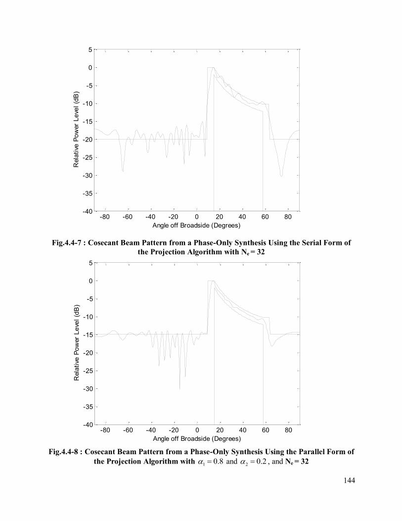
144
Fig.4.4-7 : Cosecant Beam Pattern from a Phase-Only Synthesis Using the Serial Form of
the Projection Algorithm with Ne = 32
Fig.4.4-8 : Cosecant Beam Pattern from a Phase-Only Synthesis Using the Parallel Form of
the Projection Algorithm with 1 0.8 and 2 0.2 , and Ne = 32
-80 -60 -40 -20 0 20 40 60 80-40
-35
-30
-25
-20
-15
-10
-5
0
5
Angle off Broadside (Degrees)
Rela
tive
Po
wer
Le
vel
(dB
)
-80 -60 -40 -20 0 20 40 60 80-40
-35
-30
-25
-20
-15
-10
-5
0
5
Angle off Broadside (Degrees)
Rela
tive
Po
wer
Le
vel
(dB
)
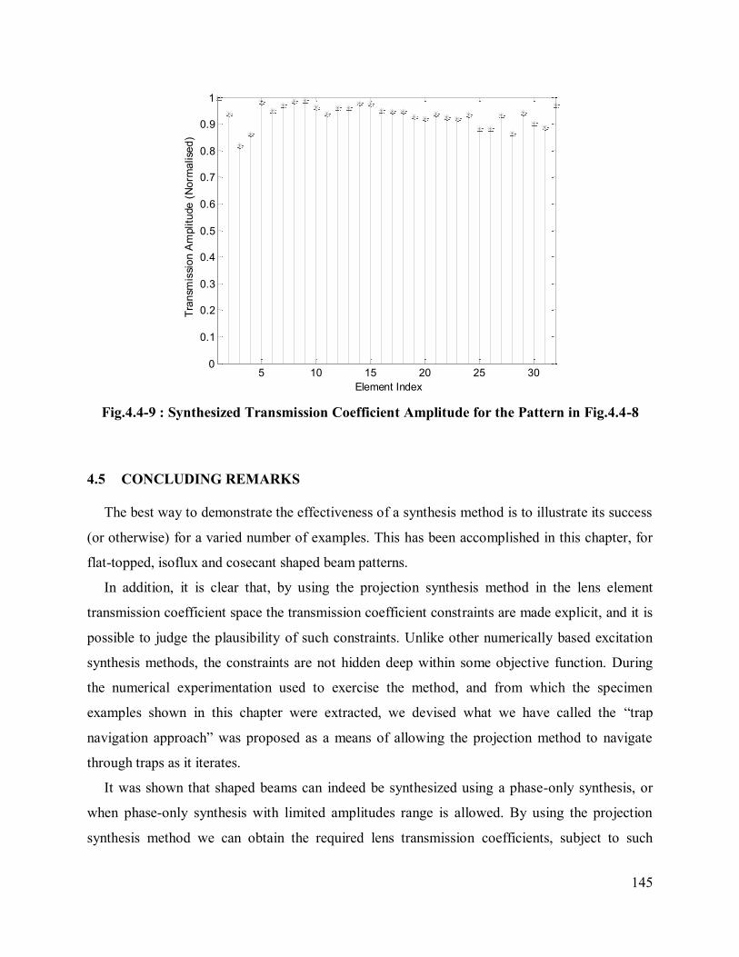
145
Fig.4.4-9 : Synthesized Transmission Coefficient Amplitude for the Pattern in Fig.4.4-8
4.5 CONCLUDING REMARKS
The best way to demonstrate the effectiveness of a synthesis method is to illustrate its success
(or otherwise) for a varied number of examples. This has been accomplished in this chapter, for
flat-topped, isoflux and cosecant shaped beam patterns.
In addition, it is clear that, by using the projection synthesis method in the lens element
transmission coefficient space the transmission coefficient constraints are made explicit, and it is
possible to judge the plausibility of such constraints. Unlike other numerically based excitation
synthesis methods, the constraints are not hidden deep within some objective function. During
the numerical experimentation used to exercise the method, and from which the specimen
examples shown in this chapter were extracted, we devised what we have called the “trap
navigation approach” was proposed as a means of allowing the projection method to navigate
through traps as it iterates.
It was shown that shaped beams can indeed be synthesized using a phase-only synthesis, or
when phase-only synthesis with limited amplitudes range is allowed. By using the projection
synthesis method we can obtain the required lens transmission coefficients, subject to such
5 10 15 20 25 300
0.1
0.2
0.3
0.4
0.5
0.6
0.7
0.8
0.9
1
Element Index
Tra
nsm
issi
on
Am
plitu
de
(N
orm
alise
d)
146
amplitude and phase constraints, that will provide a pattern that is only slightly degraded
compared to the idealized case that is physically possible without such constraints.
There are no commercial software packages for performing synthesis subject to excitation
constraints, and none for shaped beam synthesis even without excitation constraints. Thus all the
codes used in the generation of the results presented in this chapter have been developed “from
scratch” as part of the work of this thesis.
4.6 REFERENCES FOR CHAPTER 4
[1] MATLABTM
, Mathworks Inc., USA (www.mathworks.com)
[2] N. Gagnon, RF Technologies, Communications Research Centre Canada, Private
Communication.
147
CHAPTER 5
General Conclusions
The principal contributions of this thesis are:
The development of a means of formulating generalized projection based synthesis
methods that directly use the printed lens transmission coefficients as the synthesis
variables. This makes it possible to immediately perceive what influence constraints on
the actual transmission coefficients have on the possible radiation pattern performance.
A demonstration of what is physically possible as regards the performance of a
cylindrical lens antenna for three different types of widely-used shaped beams (sector
beam, cosecant beam, and isoflux beam), when either the transmission coefficient
amplitudes, or transmission phases, or both, are restricted in some way. It appears that
this is the first time that shaped beam synthesis subject to the variety of transmission
coefficient constraints has been reported, and certainly so for the phase-only synthesis of
such shaped beams.
In order to achieve the above-mentioned syntheses the projection method was
implemented in both a serial and parallel form. In the present context (where we only use
one pattern constraint operator and one transmission coefficient constraint operator in any
synthesis process) these provide almost the same results. This is the first time a parallel
version has been used in the projection synthesis of shaped beam antennas (albeit only
using two projection operators, one for the pattern and the other for the transmission
coefficient constraints). We believe it offers the advantage of performing a synthesis that
provides an indication of what constraints can be tolerated without sacrificing too much
as far as the pattern requirements are concerned, through judicious use of the
multiplicative weights on the two operators. We saw in Section 2.7 that the parallel
version can in fact incorporate several different projection operators; this might be used
to good effect such as synthesizing a lens that simultaneously provides different beam
types, one for each of two (or more) offset feeds, to name just one possibility.
148
We have defined a new projection operator that constraints the transmission coefficient to
values that must be selected from a set of available transmission coefficients. This allows
what we have referred to as an “opportunistic synthesis”. Transmission coefficient
constraints of any kind can be effectively imposed by simply removing from the database
transmission coefficient values that are not allowed.
The development of an effective method to find sets of starting values of the transmission
coefficients that will allow the projection synthesis algorithm to progress as it begins
iterating. The method can be applied to any shaped beam pattern for which an ideal
pattern shape is properly defined. Good starting values are crucial for the success of
projection synthesis methods.
We have also proposed and used what we have called the “trap navigation approach” to
prevent the projection synthesis algorithm from stagnating at a trap.
There remain some issues whose investigation in the future would prove useful:
Recently65
a type of reflectarray antenna element has been devised where elements are
selected not only for their correct reflection coefficient phases but also their geometrical
similarity. If it were possible to use a similar approach to set up a database of printed lens
elements (transmitarray elements), where more than one geometrical shape is available to
give the same complex transmission coefficient value, then a projection synthesis method
could be formulated to simultaneously synthesize the required shaped beam pattern and
select elements so that each is surrounded by elements similar to it. We suspect that
parallel form of the projection algorithm would be applicable.
Another obvious suggestion for future work is to extend the synthesis procedure to apply
to lens antennas which are not cylindrical (with a shaped beam in one pattern plane) but
fully three-dimensional. This would require the forward operator to be derived for planar
arrays of cells; this would be a relatively straightforward now that the form is know for
65 J.Ethier, et al., “Reflectarray Design Using Similarity-Shaped Fragmented Sub-Wavelength Elements”,
Electronics Letters, Vol.48, No.15, pp.900-902, July 2012.

149
the cylindrical lens case from the present work. New starting value estimation details
would be needed, but the method devised here can be so generalized.
We have used the weight vector (in the reverse operator) in a simple fashion, namely by
setting it equal to a higher value in the shaped beam region than the sidelobe region if
necessary. It might be preferable to use it in an adaptive way, as follows : At the end of
each iteration of the projection method search for only those sample angles where the
pattern violates the shaped beam mask. During the next iteration set the weights
corresponding to only these angles to values larger than unity.
More general feed models could be incorporated that allow an offset feed to be used. The
feed could then possibly be used to “help” the lens in providing a phase tilt when
asymmetrical patterns such as the cosecant case, are desired, and perhaps achieve a
pattern performance (when transmission coefficient amplitude and phase constraints are
imposed) that are closer to that when no such constraints are imposed.
In order to avoid large discontinuities in the printed lens conductor patterns we would
want to constrain the smoothness of the amplitude and phase distributions. Projection
operators should be sought to enforce such smoothness conditions within the projection
synthesis framework. We suspect that this might be possible using a parallel version of
the algorithm.
A projection operator that could be used to minimise the tolerance sensitivity of a
resulting synthesized excitation set would be useful to arrive at printed lens antennas for
which a varying feed field incidence angle from element to element matters less as far as
the element transmission coefficient value is concerned.