Fluid Dynamics And Turbo Machines. Professor Dr …textofvideo.nptel.ac.in/112106200/lec1.pdf · So let us look at the slides now. So what you can see here, let us see what we actually

Fluid Dynamics And Turbo Machines.Professor Dr Shamit Bakshi.

Department Of Mechanical Engineering.Indian Institute Of Technology Madras.

Part A.Module-1.Lecture-1.

Introduction To Fluid Flow.

Good morning and welcome to this course on fluid dynamics and turbo machines. This

course will be taught into modules, the 1st module is on fluid dynamics, the 2nd one is on turbo

machines, the 1st part, the 1st module will be taught by me, I am Dr Shamit Bakshi. Tthe 2nd

part which deals with turbo machines will be taught by Dr Dhiman Chatterjee. In this 1 st

module, I have divided it into 4 parts, so we will begin, the 1 st part is actually on introduction

to fluid flow. So, this will be, the lectures which will be given during the 1st week of this

course. So, we will start with the 1st lecture.

(Refer Slide Time: 1:59)

So, what, let us look at the slides now. So what you can see here, let us see what we actually

mean by a fluid flow and what are the applications, why do we need to study fluid flow. So,

this is basically, what you see here these arrows pointing towards right, these are these are

indicative of a flow, in the sense these are like velocity vector. Velocity is a vector quantity,

so we indicate it by both magnitude and the direction. So, this is like a flow. Now, let say we

have a plate, a flat plate in front of this flow, so what happens? This is easy to imagine what

will happen and we all know that the flow starts acting on the plate and the plate starts

moving. I am sorry, so the plate starts moving in the direction of the flow.


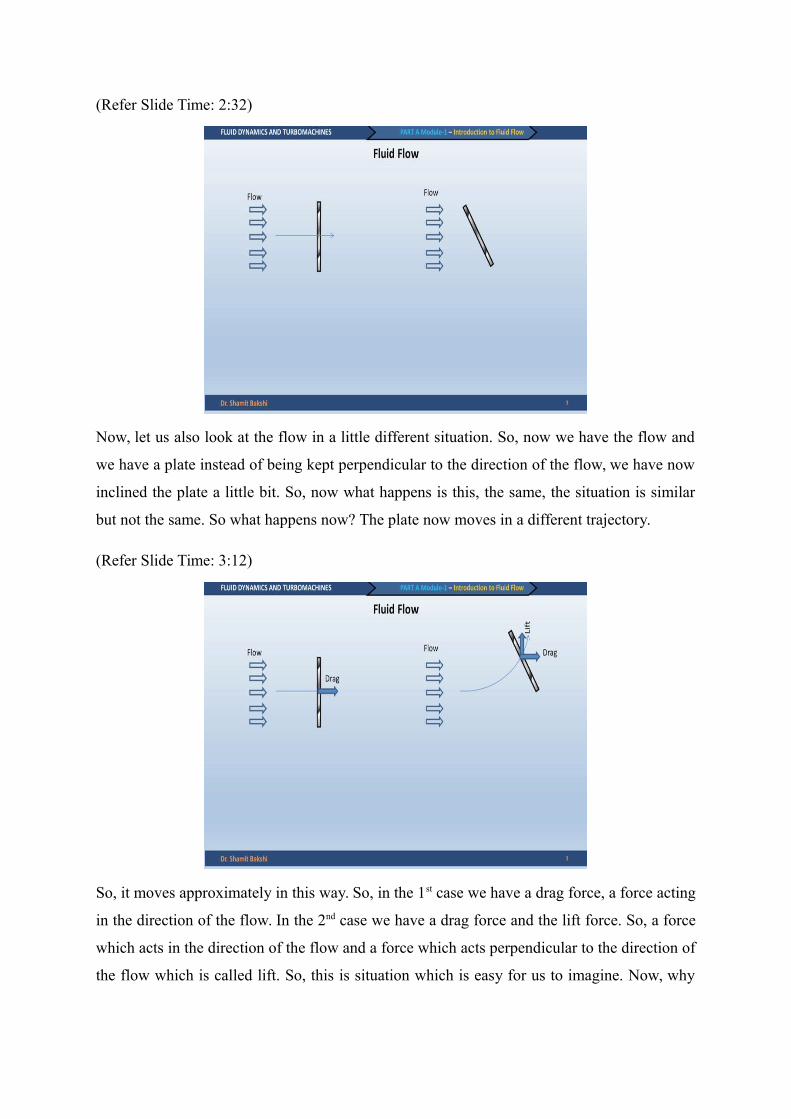
Now, let us also look at the flow in a little different situation. So, now we have the flow and

we have a plate instead of being kept perpendicular to the direction of the flow, we have now

inclined the plate a little bit. So, now what happens is this, the same, the situation is similar

but not the same. So what happens now? The plate now moves in a different trajectory.


So, it moves approximately in this way. So, in the 1st case we have a drag force, a force acting

in the direction of the flow. In the 2nd case we have a drag force and the lift force. So, a force

which acts in the direction of the flow and a force which acts perpendicular to the direction of

the flow which is called lift. So, this is situation which is easy for us to imagine. Now, why

do, what interests us to study this kind of situation or or this kind of flows is that if we can

study fluid mechanics or fluid dynamics, we can answer some questions.

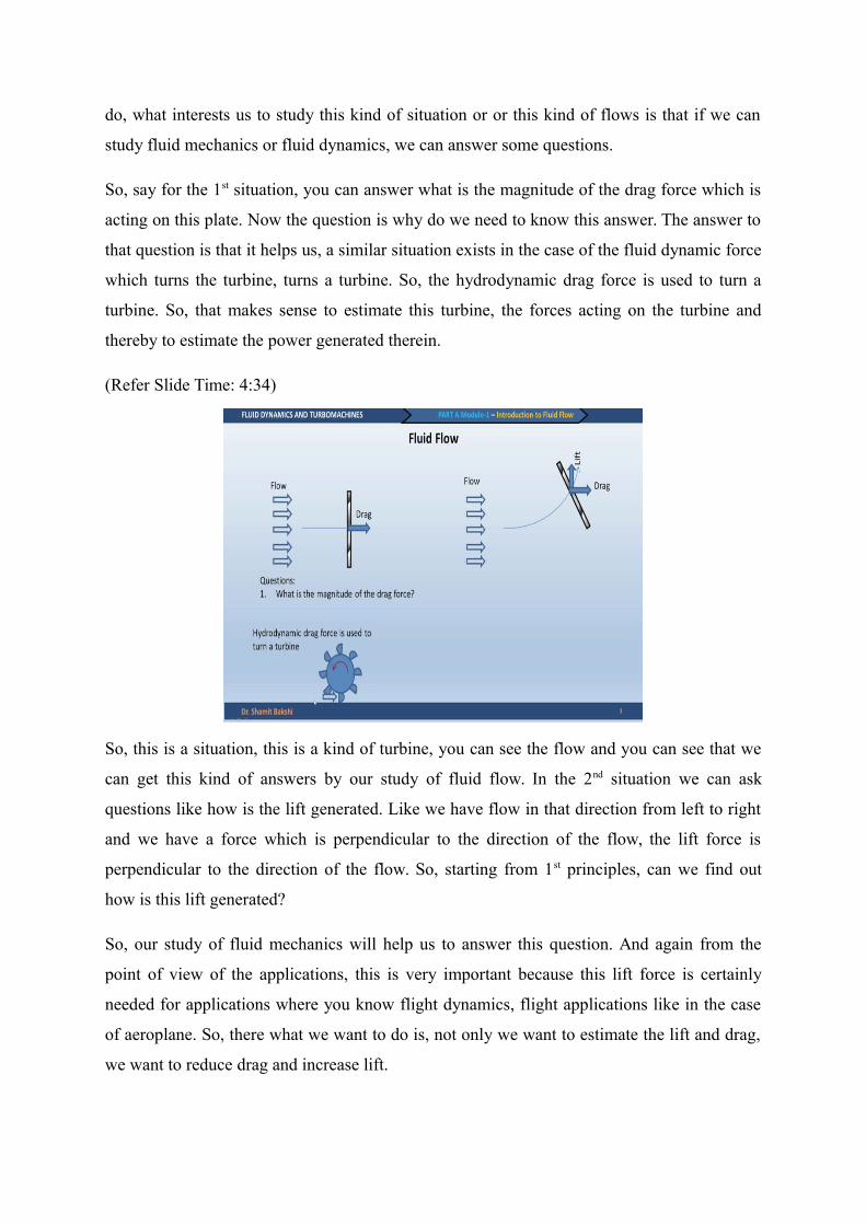
So, say for the 1st situation, you can answer what is the magnitude of the drag force which is

acting on this plate. Now the question is why do we need to know this answer. The answer to

that question is that it helps us, a similar situation exists in the case of the fluid dynamic force

which turns the turbine, turns a turbine. So, the hydrodynamic drag force is used to turn a

turbine. So, that makes sense to estimate this turbine, the forces acting on the turbine and

thereby to estimate the power generated therein.


So, this is a situation, this is a kind of turbine, you can see the flow and you can see that we

can get this kind of answers by our study of fluid flow. In the 2nd situation we can ask

questions like how is the lift generated. Like we have flow in that direction from left to right

and we have a force which is perpendicular to the direction of the flow, the lift force is

perpendicular to the direction of the flow. So, starting from 1st principles, can we find out

how is this lift generated?

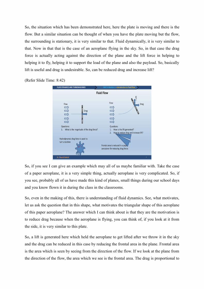
So, our study of fluid mechanics will help us to answer this question. And again from the

point of view of the applications, this is very important because this lift force is certainly

needed for applications where you know flight dynamics, flight applications like in the case

of aeroplane. So, there what we want to do is, not only we want to estimate the lift and drag,

we want to reduce drag and increase lift.

So, the situation which has been demonstrated here, here the plate is moving and there is the

flow. But a similar situation can be thought of when you have the plate moving but the flow,

the surrounding is stationary, it is very similar to that. Fluid dynamically, it is very similar to

that. Now in that that is the case of an aeroplane flying in the sky. So, in that case the drag

force is actually acting against the direction of the plane and the lift force in helping to

helping it to fly, helping it to support the load of the plane and also the payload. So, basically

lift is useful and drag is undesirable. So, can be reduced drag and increase lift?


So, if you see I can give an example which may all of us maybe familiar with. Take the case

of a paper aeroplane, it is a very simple thing, actually aeroplane is very complicated. So, if

you see, probably all of us have made this kind of planes, small things during our school days

and you know flown it in during the class in the classrooms.

So, even in the making of this, there is understanding of fluid dynamics. See, what motivates,

let us ask the question that in this shape, what motivates the triangular shape of this aeroplane

of this paper aeroplane? The answer which I can think about is that they are the motivation is

to reduce drag because when the aeroplane is flying, you can think of, if you look at it from

the side, it is very similar to this plate.

So, a lift is generated here which held the aeroplane to get lifted after we throw it in the sky

and the drag can be reduced in this case by reducing the frontal area in the plane. Frontal area

is the area which is seen by seeing from the direction of the flow. If we look at the plane from

the direction of the flow, the area which we see is the frontal area. The drag is proportional to

the frontal area and that can be reduced if we use a triangular shape instead of a rectangular

shape here.

So, that motivates the design, the small which unconsciously we take this kind of shape and

we see that this helps us to explain, the fluid dynamics helps us to explain the shape. So, you

can easily think up think of the kind of aerodynamics which is, which goes into the

understanding of aerodynamics which goes into making of a real aeroplane, if this is only a

paper aeroplane.

These 2 examples, one that of turbine and another that of an aeroplane which we took are just

2 examples and you can cite numerous examples on applications of fluid flow starting from

microfluidics to very large scale flows. And so you can easily understand that this has a wide

range of application, fluid dynamics as a wide range of applications.


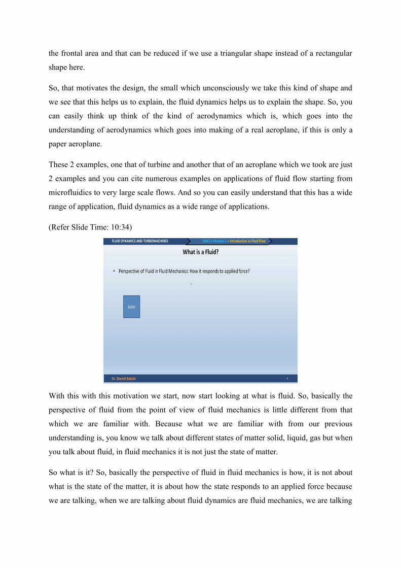
With this with this motivation we start, now start looking at what is fluid. So, basically the

perspective of fluid from the point of view of fluid mechanics is little different from that

which we are familiar with. Because what we are familiar with from our previous

understanding is, you know we talk about different states of matter solid, liquid, gas but when

you talk about fluid, in fluid mechanics it is not just the state of matter.

So what is it? So, basically the perspective of fluid in fluid mechanics is how, it is not about

what is the state of the matter, it is about how the state responds to an applied force because

we are talking, when we are talking about fluid dynamics are fluid mechanics, we are talking

about forces. So, the definition of fluid is very much related to the applied force. So, that

means fluid responds differently than solids when a force is applied to it.


So, now let us take an example of a solid and when we have said the applied force, you can

have 2 situations. You can apply a normal force like what is shown here, that means the

duration of the force is perpendicular to the direction of to the surface on which it is acting.

So, this is a purely normal force. So, let us see how the solid it is known to us, if we apply

this force, the solid changes its volume and when you withdraw this force, it comes back to

its original shape and size. Of course this is only true if the force which we have applied is

within, it keeps the solid within its elastic limit. So, what we say is that solid actually behaves

elastically on application of a force, on application of a normal force.


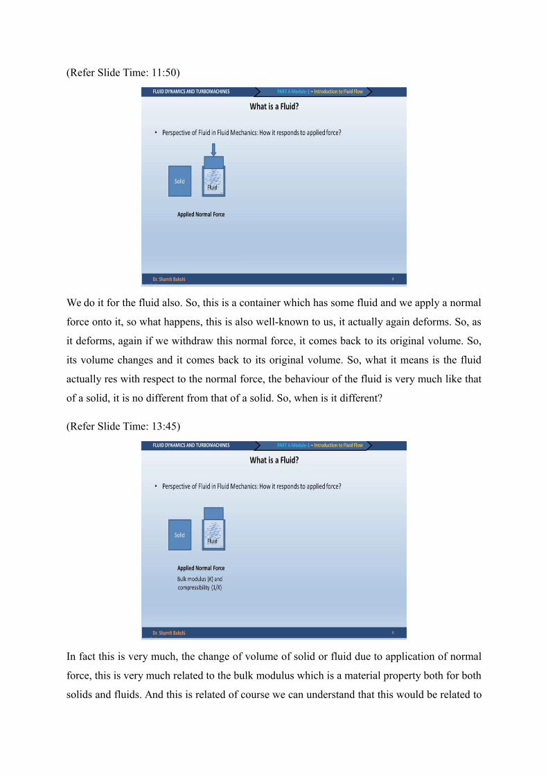
We do it for the fluid also. So, this is a container which has some fluid and we apply a normal

force onto it, so what happens, this is also well-known to us, it actually again deforms. So, as

it deforms, again if we withdraw this normal force, it comes back to its original volume. So,

its volume changes and it comes back to its original volume. So, what it means is the fluid

actually res with respect to the normal force, the behaviour of the fluid is very much like that

of a solid, it is no different from that of a solid. So, when is it different?


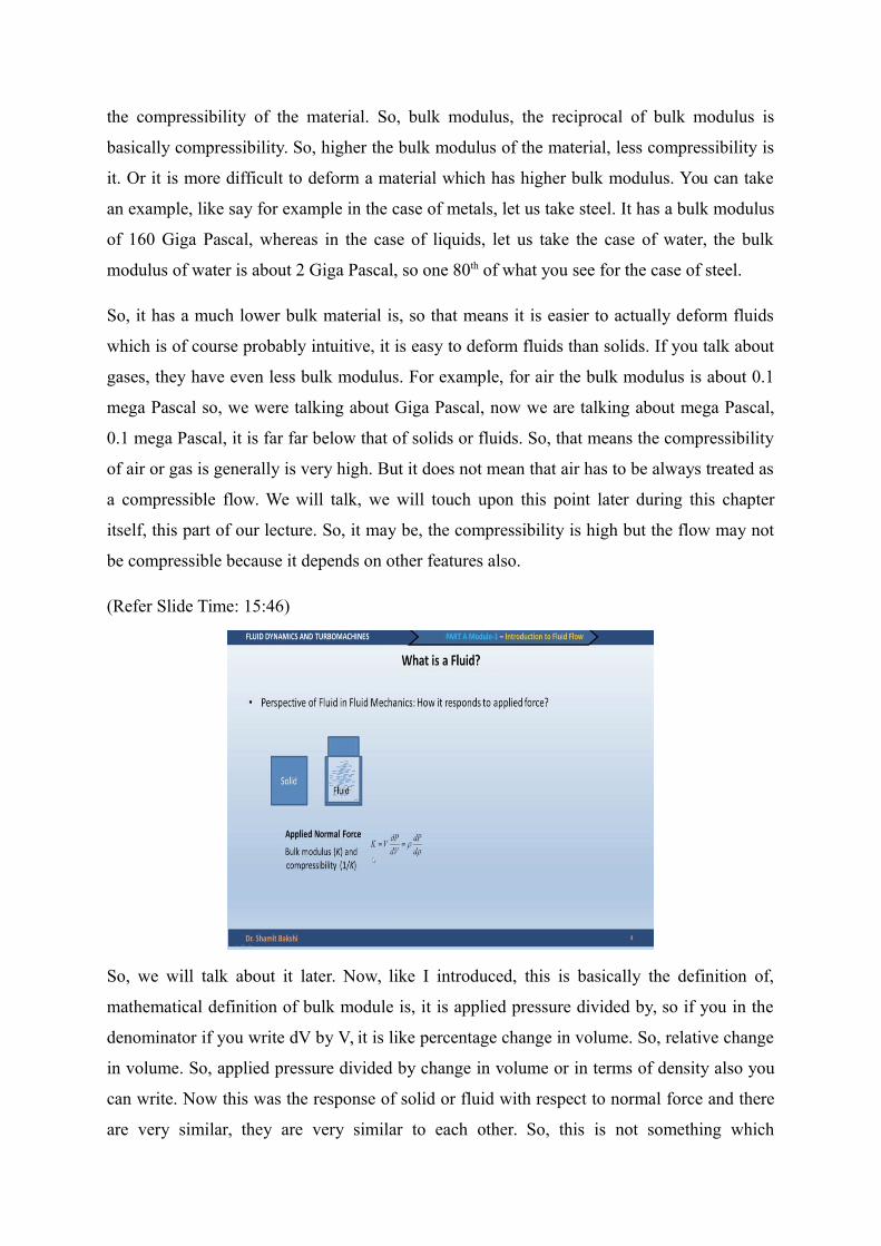
In fact this is very much, the change of volume of solid or fluid due to application of normal

force, this is very much related to the bulk modulus which is a material property both for both

solids and fluids. And this is related of course we can understand that this would be related to

the compressibility of the material. So, bulk modulus, the reciprocal of bulk modulus is

basically compressibility. So, higher the bulk modulus of the material, less compressibility is

it. Or it is more difficult to deform a material which has higher bulk modulus. You can take

an example, like say for example in the case of metals, let us take steel. It has a bulk modulus

of 160 Giga Pascal, whereas in the case of liquids, let us take the case of water, the bulk

modulus of water is about 2 Giga Pascal, so one 80th of what you see for the case of steel.

So, it has a much lower bulk material is, so that means it is easier to actually deform fluids

which is of course probably intuitive, it is easy to deform fluids than solids. If you talk about

gases, they have even less bulk modulus. For example, for air the bulk modulus is about 0.1

mega Pascal so, we were talking about Giga Pascal, now we are talking about mega Pascal,

0.1 mega Pascal, it is far far below that of solids or fluids. So, that means the compressibility

of air or gas is generally is very high. But it does not mean that air has to be always treated as

a compressible flow. We will talk, we will touch upon this point later during this chapter

itself, this part of our lecture. So, it may be, the compressibility is high but the flow may not

be compressible because it depends on other features also.


So, we will talk about it later. Now, like I introduced, this is basically the definition of,

mathematical definition of bulk module is, it is applied pressure divided by, so if you in the

denominator if you write dV by V, it is like percentage change in volume. So, relative change

in volume. So, applied pressure divided by change in volume or in terms of density also you

can write. Now this was the response of solid or fluid with respect to normal force and there

are very similar, they are very similar to each other. So, this is not something which

distinguishes a solid from a fluid. So, what distinguishes solid from a fluid will be understood

better if we now take the same solid and we apply a shear force. So, now we apply a shear

force.


The shear force is parallel to the surface. Okay. So when we apply a shear force to the solid,

what is the behaviour, this is also quite understandable and it is quite also intuitive. So, we

apply the shear force, the solid again deforms and when you withdraw this, it comes back to

its original shape.


So, in this case, solid behaves actually, again of course the applied shear should be within the

elastic limit of the solid. So, again the solid, even under the application of a shear force

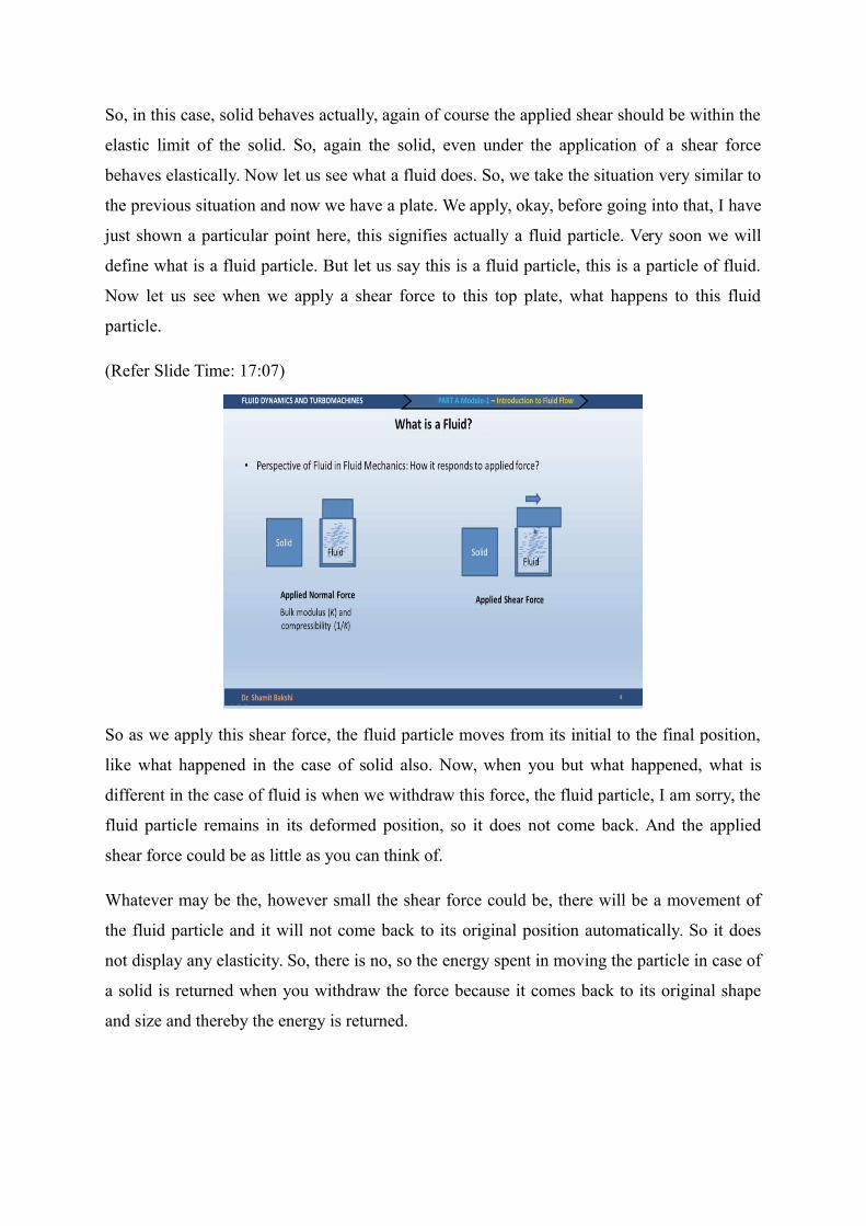
behaves elastically. Now let us see what a fluid does. So, we take the situation very similar to

the previous situation and now we have a plate. We apply, okay, before going into that, I have

just shown a particular point here, this signifies actually a fluid particle. Very soon we will

define what is a fluid particle. But let us say this is a fluid particle, this is a particle of fluid.

Now let us see when we apply a shear force to this top plate, what happens to this fluid

particle.


So as we apply this shear force, the fluid particle moves from its initial to the final position,

like what happened in the case of solid also. Now, when you but what happened, what is

different in the case of fluid is when we withdraw this force, the fluid particle, I am sorry, the

fluid particle remains in its deformed position, so it does not come back. And the applied

shear force could be as little as you can think of.

Whatever may be the, however small the shear force could be, there will be a movement of

the fluid particle and it will not come back to its original position automatically. So it does

not display any elasticity. So, there is no, so the energy spent in moving the particle in case of

a solid is returned when you withdraw the force because it comes back to its original shape

and size and thereby the energy is returned.


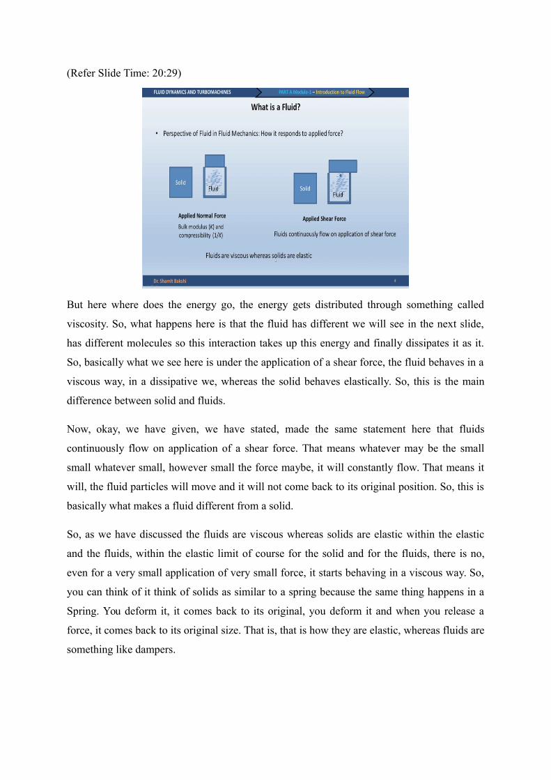
But here where does the energy go, the energy gets distributed through something called

viscosity. So, what happens here is that the fluid has different we will see in the next slide,

has different molecules so this interaction takes up this energy and finally dissipates it as it.

So, basically what we see here is under the application of a shear force, the fluid behaves in a

viscous way, in a dissipative we, whereas the solid behaves elastically. So, this is the main

difference between solid and fluids.

Now, okay, we have given, we have stated, made the same statement here that fluids

continuously flow on application of a shear force. That means whatever may be the small

small whatever small, however small the force maybe, it will constantly flow. That means it

will, the fluid particles will move and it will not come back to its original position. So, this is

basically what makes a fluid different from a solid.

So, as we have discussed the fluids are viscous whereas solids are elastic within the elastic

and the fluids, within the elastic limit of course for the solid and for the fluids, there is no,

even for a very small application of very small force, it starts behaving in a viscous way. So,

you can think of it think of solids as similar to a spring because the same thing happens in a

Spring. You deform it, it comes back to its original, you deform it and when you release a

force, it comes back to its original size. That is, that is how they are elastic, whereas fluids are

something like dampers.


So it gets dissipated, the energy which you spend on the fluid, it gets dissipated like in the

case of a damper. It is not like that all the materials which we see are around us, if we have to

define it in a, in the language of fluid mechanics, we can distinguish them into only 2

divisions like solids and solids and fluids, or viscous or elastic, elastic and viscous. There are

materials which have a combination of both, those are known as viscoelastic materials. Very

good example of these are biological tissues.

So, what happens is when you apply a force on this, they undergo some, they undergo some

permanent deformation, they flow like fluid but when you release the force, it behaves to

some extent elastically. So, some energy, some part of the energy is returned through

elasticity. So, it is a combination of both. Of course if you have to talk about those materials,

you have to talk in terms of or model those materials, you have to consider both spring and

the dampers, spring and damper system.


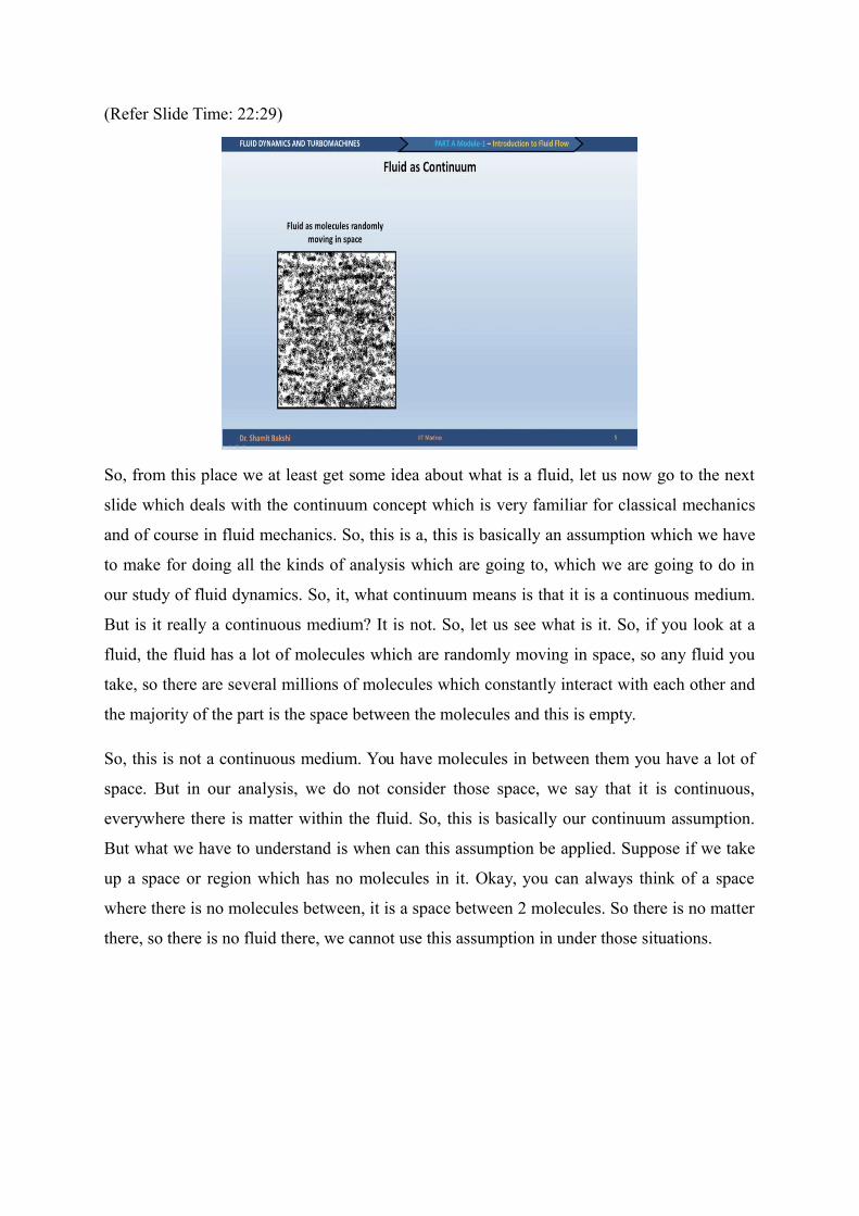
So, from this place we at least get some idea about what is a fluid, let us now go to the next

slide which deals with the continuum concept which is very familiar for classical mechanics

and of course in fluid mechanics. So, this is a, this is basically an assumption which we have

to make for doing all the kinds of analysis which are going to, which we are going to do in

our study of fluid dynamics. So, it, what continuum means is that it is a continuous medium.

But is it really a continuous medium? It is not. So, let us see what is it. So, if you look at a

fluid, the fluid has a lot of molecules which are randomly moving in space, so any fluid you

take, so there are several millions of molecules which constantly interact with each other and

the majority of the part is the space between the molecules and this is empty.

So, this is not a continuous medium. You have molecules in between them you have a lot of

space. But in our analysis, we do not consider those space, we say that it is continuous,

everywhere there is matter within the fluid. So, this is basically our continuum assumption.

But what we have to understand is when can this assumption be applied. Suppose if we take

up a space or region which has no molecules in it. Okay, you can always think of a space

where there is no molecules between, it is a space between 2 molecules. So there is no matter

there, so there is no fluid there, we cannot use this assumption in under those situations.


So, to get into little more details about that, so let us consider this volume, so this red circle

shown within the fluid domain is a small volume, let us magnify this. So if we magnify and

try to see it, it is a very small volume, so it has some counted number of molecules inside it.

Okay, if you can, it is countable, let us say 10, 11, something like that. Now, if we try to talk

about some property within this small volume, let us take an example of density as a property.

So, what happens is these molecules are not stationary molecules, they are constantly

moving, so at a particular time you might have, let us say 10 molecules, in the next time

instant, in the same volume if you look at, you might have 12 molecules, you might have 5

molecules.


So, if the volume is very small to begin with, the number of molecules within that volume

will be very small and as result of that if we have to define a property like density which is

mass of all the molecules divided by the volume, we will see that this density will vary

constantly with time. So, we cannot define a property like density in the fluid domain. This

problem will not arise if we take a little bigger volume.

So, if you see a bigger circle now, if we consider this volume and if we try to look at it, we

will see there are, there are a lot of molecules within this volume and let us say it has 10 to

the power 20 molecules. And it may so happen that in the next time instant, it has some 100

molecules more or 50 molecules less or 200 molecules less, that variation of 10 or 100 or 50

or 200 in a number of 10 to the power 20 will not make a big difference for a property like

density.

Like the total mass of the molecules divided by volume. So, we can define a property like

density of the medium. We can see it, okay, before going into the aspect of density further, we

can say that this thing which we have taken out from the fluid, which we are looking into the

fluid is essentially this minimum volume which is required to call the fluid as a fluid is

known as the fluid particle. We will keep on using this terminology time and again during our

discussion on fluid flow. So, this is the minimum volume which is required to call a fluid as

the fluid. Now we will also talk about that volume very soon.


Now let us say, we were talking about density, let us plot this density with respect to this,

with respect to delta V. What is delta V, delta V is basically this elemental volume. So, it can

be very small to big. Now, if it is very small, that the elemental volume is very small so that

the number of molecules within that volume is very less, if that is the situation and if we plot

density here, we will see that in this region there is a random fluctuation of density.

And this is due to the microscopic uncertainty in the number of molecules within that

volume, whereas if you look at, of course, if you look at a volume larger than some kind of a

threshold volume which is the volume which is required to call a, to define a fluid particle

like this that has more or less constant density. So, the density, there is no random fluctuation,

this is now, it can be defined as a property of the fluid.


Of course if you go further down, means that for larger volume, you can see that there is a

macroscopic variation or there could be a macroscopic variation of density. This could be due

to the variation in temperature. At a region where the temperature is less, the density will be

high and so on so forth. So, this macroscopic variations will not show the random

fluctuations as displayed in the region where the elemental volume was very small.

So, now this is basically delta V Prime is the minimum volume which you need to consider

for calling this material as a continuum. Now let us look at, so this is macroscopic variation

as we already discussed, this is the reason, this is the volume which you need to consider for

considering this as a continuum, the fluid is a continuum. And we will always make this

assumption in our in this course.


Now the, for a continuum, the advantage is you can define continuous fields like that of

density. You can say now I can, once I have taken this volume, I can define density at

different points within this fluid. We will very soon look at other different properties also

which can be continuously defined within the continuum. Now, the next question is that we

have showed here delta V Prime as the minimum volume which is required to call this fluid,

to treat the fluid as a continuum, what is the magnitude is of this volume? So, we have put a

question mark here to emphasise what is the condition, when can we call fluid as a

continuum? To answer this question, we will not directly deal with volume, we will rather

deal with length scale.


So there is a property, there is a parameter which is defined as Knudsen number which is

essentially the ratio of the mean free path of the molecule in the flow divided by the

characteristic length scale. Now what is mean free path? Mean free path is basically the

distance travelled by the molecule between 2 collisions. The particle, the molecules are

constantly colliding with each other, that is well-known. Now if you have very densely

packed molecules, that means high-density situation, then they will collide more frequently or

in other sense, in terms of length scale they will collide with a smaller lengths as compared to

if the fluid is rarefied, that means it is not so densely packed, the molecules are not so densely

packed.


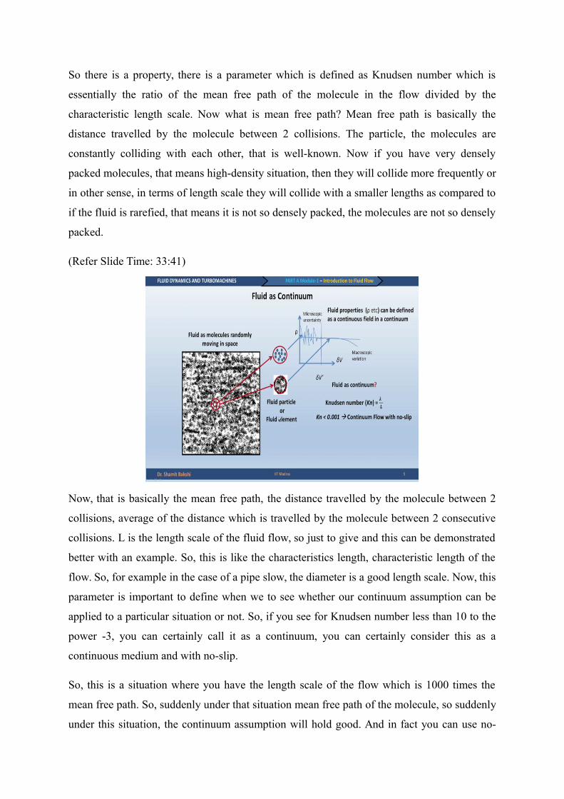
Now, that is basically the mean free path, the distance travelled by the molecule between 2

collisions, average of the distance which is travelled by the molecule between 2 consecutive

collisions. L is the length scale of the fluid flow, so just to give and this can be demonstrated

better with an example. So, this is like the characteristics length, characteristic length of the

flow. So, for example in the case of a pipe slow, the diameter is a good length scale. Now, this

parameter is important to define when we to see whether our continuum assumption can be

applied to a particular situation or not. So, if you see for Knudsen number less than 10 to the

power -3, you can certainly call it as a continuum, you can certainly consider this as a

continuous medium and with no-slip.

So, this is a situation where you have the length scale of the flow which is 1000 times the

mean free path. So, suddenly under that situation mean free path of the molecule, so suddenly

under this situation, the continuum assumption will hold good. And in fact you can use no-

slip they are there, the no-slip means that if the fluid is near to the, let us say this is a wall, if

the fluid is near to the wall, the fluid particle is near to the wall, the velocity of the fluid

particle will be same as the velocity of the wall.

But it does not mean that the molecule near the walls are stationary, they are actually

randomly moving like elsewhere. But when you define a fluid particle like this, then the net

movement of the fluid particle is 0. So, that is how, that is what we mean by no-slip

condition. What is once we get into continuum mechanics, we mostly deal with the fluid

particles and we forget about molecules, we forget about the existence of the molecules.


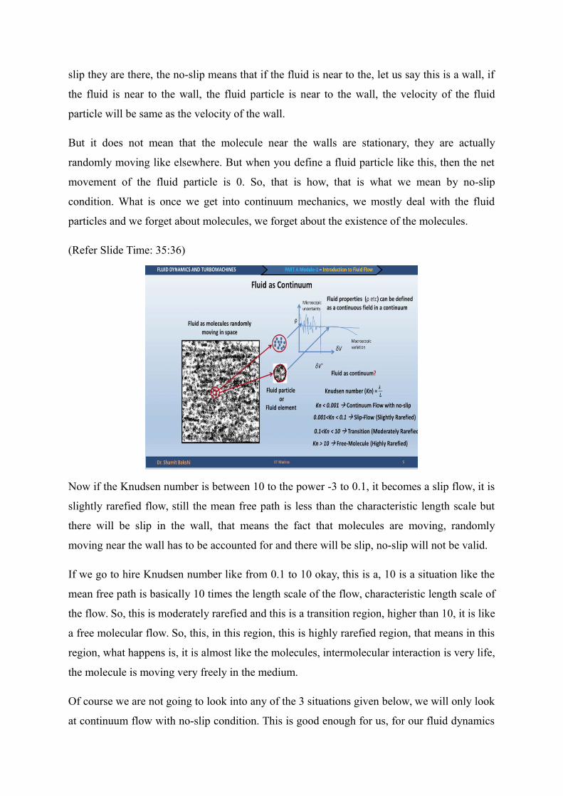
Now if the Knudsen number is between 10 to the power -3 to 0.1, it becomes a slip flow, it is

slightly rarefied flow, still the mean free path is less than the characteristic length scale but

there will be slip in the wall, that means the fact that molecules are moving, randomly

moving near the wall has to be accounted for and there will be slip, no-slip will not be valid.

If we go to hire Knudsen number like from 0.1 to 10 okay, this is a, 10 is a situation like the

mean free path is basically 10 times the length scale of the flow, characteristic length scale of

the flow. So, this is moderately rarefied and this is a transition region, higher than 10, it is like

a free molecular flow. So, this, in this region, this is highly rarefied region, that means in this

region, what happens is, it is almost like the molecules, intermolecular interaction is very life,

the molecule is moving very freely in the medium.

Of course we are not going to look into any of the 3 situations given below, we will only look

at continuum flow with no-slip condition. This is good enough for us, for our fluid dynamics

which can be used for turbo machinery applications. So, now we know about this assumption,

continuum assumption, we can we can find out, we can estimate a situation given the length

scale and find out whether we can use the continuum assumption, we can whether use, we

can use continuum, define continuum properties within a particular flow.

So, one very important property of a flow field is the velocity field because velocity is the

most important indicator of the flow. Say density you can have even without flow also but

velocity, if the velocity is there within a fluid, then the flow, the question of flow comes into

picture. So, let us see what is a velocity field. Of course we can define a velocity feel like a

density field when the continuum assumption is valid. It is not that we are not familiar with

velocity field but again the velocity field when you talk about in a fluid dynamics application

or continuum fluid dynamics application, the definition of velocity is little different from

what we are familiar with.


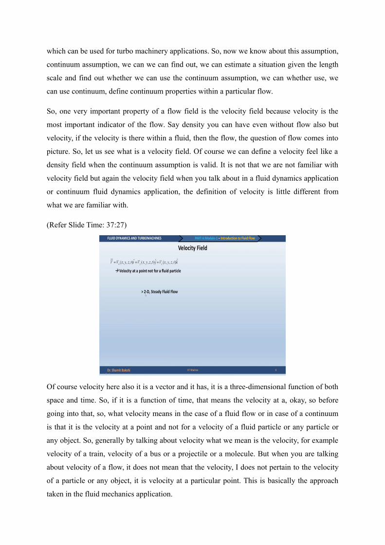
Of course velocity here also it is a vector and it has, it is a three-dimensional function of both

space and time. So, if it is a function of time, that means the velocity at a, okay, so before

going into that, so, what velocity means in the case of a fluid flow or in case of a continuum

is that it is the velocity at a point and not for a velocity of a fluid particle or any particle or

any object. So, generally by talking about velocity what we mean is the velocity, for example

velocity of a train, velocity of a bus or a projectile or a molecule. But when you are talking

about velocity of a flow, it does not mean that the velocity, I does not pertain to the velocity

of a particle or any object, it is velocity at a particular point. This is basically the approach

taken in the fluid mechanics application.

Now when we are talking about a 2-D steady fluid flow, okay that means the word steady

means that it does not change with time. Anything which is not changing with time is

basically steady, so that means this low, when it is a function of time, it is unstable. So, 2-D

means that it is only 2 velocities are nonzero, like that of Vx and Vy, let us say Vz is 0 but

that is not sufficient. To be 2-D, to be really two-dimensional, it is not sufficient is just that

the Vz is0, it is also important that VX and VY which are nonzero should not vary along Z

direction. So, VX and VY are only functions of X and Y and not function of Z. If you go

along the Z direction, VX and VY should not change, at the same time VZ is also 0.


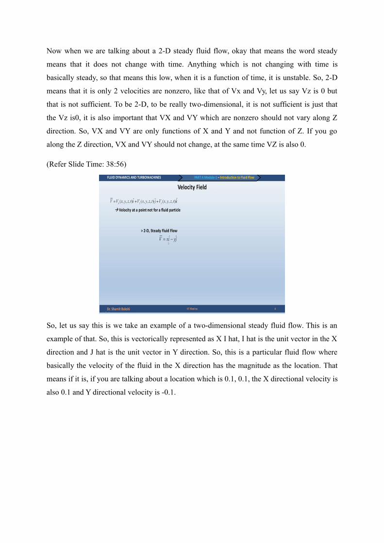
So, let us say this is we take an example of a two-dimensional steady fluid flow. This is an

example of that. So, this is vectorically represented as X I hat, I hat is the unit vector in the X

direction and J hat is the unit vector in Y direction. So, this is a particular fluid flow where

basically the velocity of the fluid in the X direction has the magnitude as the location. That

means if it is, if you are talking about a location which is 0.1, 0.1, the X directional velocity is

also 0.1 and Y directional velocity is -0.1.


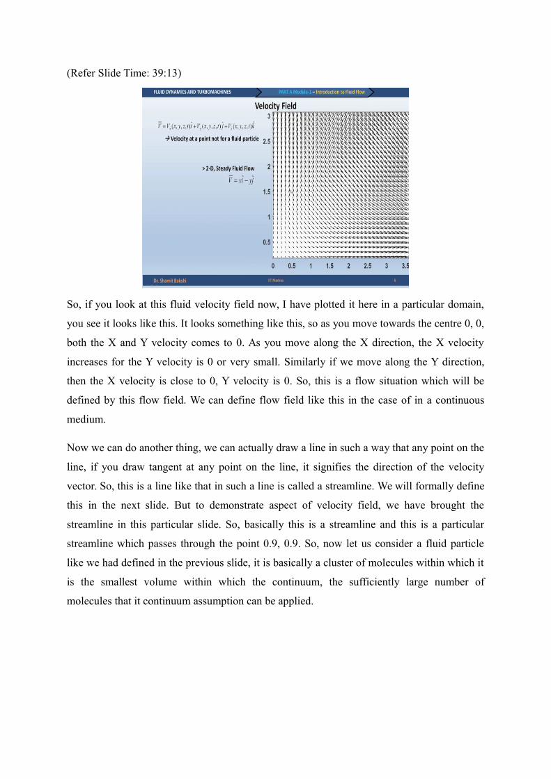
So, if you look at this fluid velocity field now, I have plotted it here in a particular domain,

you see it looks like this. It looks something like this, so as you move towards the centre 0, 0,

both the X and Y velocity comes to 0. As you move along the X direction, the X velocity

increases for the Y velocity is 0 or very small. Similarly if we move along the Y direction,

then the X velocity is close to 0, Y velocity is 0. So, this is a flow situation which will be

defined by this flow field. We can define flow field like this in the case of in a continuous

medium.

Now we can do another thing, we can actually draw a line in such a way that any point on the

line, if you draw tangent at any point on the line, it signifies the direction of the velocity

vector. So, this is a line like that in such a line is called a streamline. We will formally define

this in the next slide. But to demonstrate aspect of velocity field, we have brought the

streamline in this particular slide. So, basically this is a streamline and this is a particular

streamline which passes through the point 0.9, 0.9. So, now let us consider a fluid particle

like we had defined in the previous slide, it is basically a cluster of molecules within which it

is the smallest volume within which the continuum, the sufficiently large number of

molecules that it continuum assumption can be applied.


So, we consider a fluid particle here, the location is 0.9, 0.9, the magnitude of velocity is 0.9,

0.9, same as 0.9, -0.9 and the magnitude is like this 0.9 square, square root of 0.9 square like

any vector quantity. So because this is a steady flow, the any particle will actually follow the

streamline. It will go along the streamline. Why will it go along the streamline? Because see,

the streamline has one particular property that particular to the streamline there is no flow.

Because there cannot be any flow as the direction tangent to the streamline is the duration of

the flow. So, normal to the streamline there is no component of velocity and as a result of that

there is no flow.


So, if there is no flow in the direction perpendicular to the streamline, so under steady state

situation when the streamline is not changing with time, the fluid particle has no choice rather

than other than following the streamline itself. So it just follows the streamline. So, we have

marked one fluid particle at the point 0.9, 0.9. Let us see a 2nd instant here, so the fluid

particle actually moves along the streamline and comes to this position. As it comes to this

position, the new position which is 3, 0.275, what has it done? It has actually accelerated in X

direction because it is initial X velocity was 0.9 and the final X velocity is 3 in some units, let

us say meter per second. So, it has accelerated in X direction but in the Y direction, the

velocity has changed from -0.9 to -0.275.

So, it has decelerated in the Y direction. So, this brings a very important discussion that the

fluid particle actually accelerates or decelerates in a flow even if the flow is steady according

to a definition of velocity, because the velocity field which we have defined is not the

velocity of the fluid particle, it is a velocity at a particular point. So, in this particular case, it

is a steady velocity, it does not it is not changing with time but the fluid particles are

accelerating or decelerating. That is why when we, but in a in general what happens is if we

talk about acceleration or deceleration, it is actually a time derivative of velocity.

But in this case we have two defined acceleration in a little different way so that we can

accommodate the acceleration of the fluid particle because the acceleration is there, a

definition of fluid particles, a definition of velocity which is defined at a point now and not

for a particle should not make the acceleration zero. So the acceleration in this case, when the

velocity is defined at a point and not that of a fluid particle has to be defined in a different

way which we will introduce in the next chapter. Now if you look at this approach in which

the velocity is defined at a point and not for a particle, this approach is called Eulerian

approach. This particular approach in continuum mechanics which is used in continuum

mechanics is called Eulerian approach. We do not bother about how the particles, what is the

particle velocity, we bother about what is the velocity at a particular point.

The second approach is something which of course we are familiar with, where we just

follow the fluid particle is called Lagrangian approach. We find out the velocity of the fluid

particle at each point. So, according to the Lagrangian approach, the velocity in this case is

changing with time, whereas in the case of Eulerian approach, the velocity is independent of

time, it is a steady velocity. So, the definitions of acceleration in the Eulerian approach is

from that in the case of Lagrangian approach. So, after getting into the fact, after getting into

the continuum assumptions and seeing that a continuous field can be only defined if the

continuum assumption is valid, we have also introduced be important parameter, one

important characteristic of the flow that this is the velocity field.

So, this brings us to the end of the first lecture where we have, the first lecture deals with the

first part of the introduction to fluid flow where here we have introduced, we have initially

seen our motivation to study fluid mechanics of fluid dynamics and then we have discussed

about what is a fluid and then introduced fluid as a continuum, the assumption, the continuum

assumption which is made for the study of fluid dynamics. We have also introduced

parameters like density field and velocity field and the two important approaches used in used

in relation to fluid flow namely the Eulerian approach and the LagrangiSan approach.

In the Eulerian approach we look at a particular, we focus our attention at a particular point

and look at the property at that point like density at that point all velocity at that point

whereas in the case of Lagrangian approach, we follow a fluid particle, a particle and look at

the property of the particle like position, velocity, diameter or time, sorry, the temperature of

that particular particle. Thank you.

Documents

Fluid Dynamics And Turbo Machines. Professor Dr …textofvideo.nptel.ac.in/112106200/lec1.pdf · So let us look at the slides now. So what you can see here, let us see what we actually