Computer Networks Prof. Sujoy Ghosh Department of …textofvideo.nptel.ac.in/106105081/lec17.pdf · Now let us look at link utilization in Stop and Wait – how much we are utilizing

Computer Networks Prof. Sujoy Ghosh

Department of Computer Science & Engineering Indian Institute of Technology, Kharagpur

Lecture Name - 17 Stop & Wait Protocol

Good day. So in the last lecture we were discussing about Stop and Wait Protocol. It is really a simple kind of protocol, which is used both for error control as well as for flow control in some cases. This is the simple protocol we will look at its performance now. So we will first finish our discussion on this Stop and Wait Protocol. (Refer Slide Time: 01: 06)

And this we have already seen. So each sender station sends one packet which are ACK if it is comes with some error it may send negative acknowledgement. It may not arrive at all in that case the sender will time out; in either case, that is, when it is getting a negative acknowledgement or whether it is getting a time out it will retransmit that frame transmitted earlier. The point to note is that there is only one frame, which is in transit in the channel at any point of time, whether it is the frame or the acknowledgment or the negative acknowledgement. So this is the Stop and Wait ARQ, which we have automatic repeat request we have already discussed this.

(Refer Slide Time: 01:12)


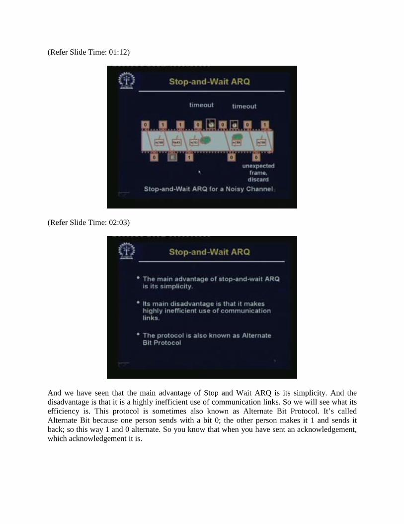
And we have seen that the main advantage of Stop and Wait ARQ is its simplicity. And the disadvantage is that it is a highly inefficient use of communication links. So we will see what its efficiency is. This protocol is sometimes also known as Alternate Bit Protocol. It’s called Alternate Bit because one person sends with a bit 0; the other person makes it 1 and sends it back; so this way 1 and 0 alternate. So you know that when you have sent an acknowledgement, which acknowledgement it is.


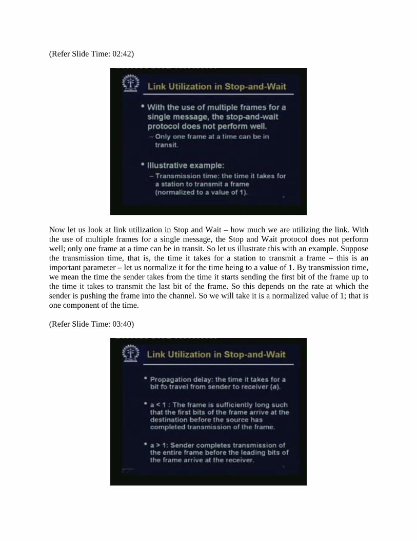
Now let us look at link utilization in Stop and Wait – how much we are utilizing the link. With the use of multiple frames for a single message, the Stop and Wait protocol does not perform well; only one frame at a time can be in transit. So let us illustrate this with an example. Suppose the transmission time, that is, the time it takes for a station to transmit a frame – this is an important parameter – let us normalize it for the time being to a value of 1. By transmission time, we mean the time the sender takes from the time it starts sending the first bit of the frame up to the time it takes to transmit the last bit of the frame. So this depends on the rate at which the sender is pushing the frame into the channel. So we will take it is a normalized value of 1; that is one component of the time. (Refer Slide Time: 03:40)

And the other component is the propagation delay, the time it takes for a bit to travel from the sender to the receiver. There will be always be a finite propagation delay, because, depending on how long the channel is, depending may be on the distance, or the speed at which the signal travels, etc., there will be a propagation delay – the time it takes for the first or any bit to move from the source to the destination. Let us call this A. Now if A less than1 – remember we have normalized our transmission time to 1 – which means that the first bit of the frame has already reached the receiver when some of the latter bits are being sent by the sender. So the frame is sufficiently long such that the first bits of the frame arrive at the destination before the source has completed transmission of the frame. And if A greater than1, that means the sender completes transmission of the entire frame before leading bits of the frame arrive at the receiver. Of course, the sender now has to wait for the acknowledgement to arrive. (Refer Slide Time: 04:59)

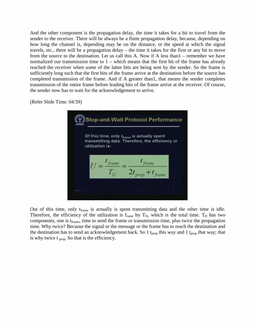
Out of this time, only tframe is actually is spent transmitting data and the other time is idle. Therefore, the efficiency of the utilization is frame by TD, which is the total time. TD has two components, one is tframe, time to send the frame or transmission time, plus twice the propagation time. Why twice? Because the signal or the message or the frame has to reach the destination and the destination has to send an acknowledgement back. So 1 tprop this way and 1 tprop that way; that is why twice t prop. So that is the efficiency.


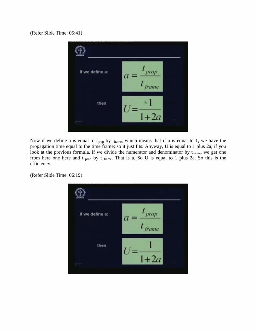
Now if we define a is equal to tprop by tframe, which means that if a is equal to 1, we have the propagation time equal to the time frame; so it just fits. Anyway, U is equal to 1 plus 2a; if you look at the previous formula, if we divide the numerator and denominator by tframe, we get one from here one here and t prop by t frame. That is a. So U is equal to 1 plus 2a. So this is the efficiency. (Refer Slide Time: 06:19)


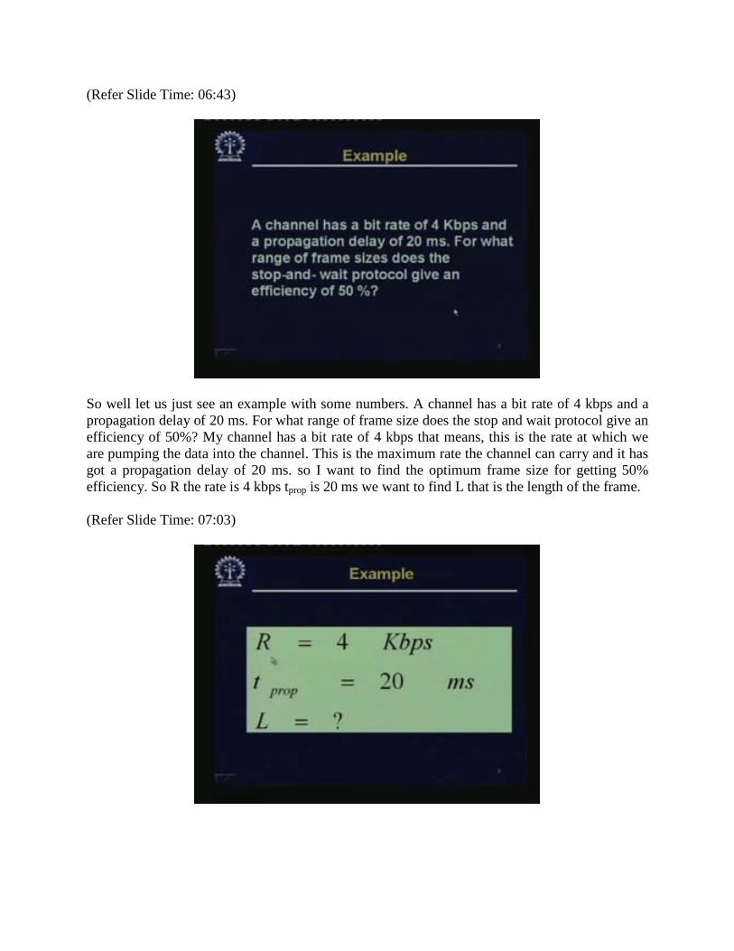
So well let us just see an example with some numbers. A channel has a bit rate of 4 kbps and a propagation delay of 20 ms. For what range of frame size does the stop and wait protocol give an efficiency of 50%? My channel has a bit rate of 4 kbps that means, this is the rate at which we are pumping the data into the channel. This is the maximum rate the channel can carry and it has got a propagation delay of 20 ms. so I want to find the optimum frame size for getting 50% efficiency. So R the rate is 4 kbps tprop is 20 ms we want to find L that is the length of the frame. (Refer Slide Time: 07:03)


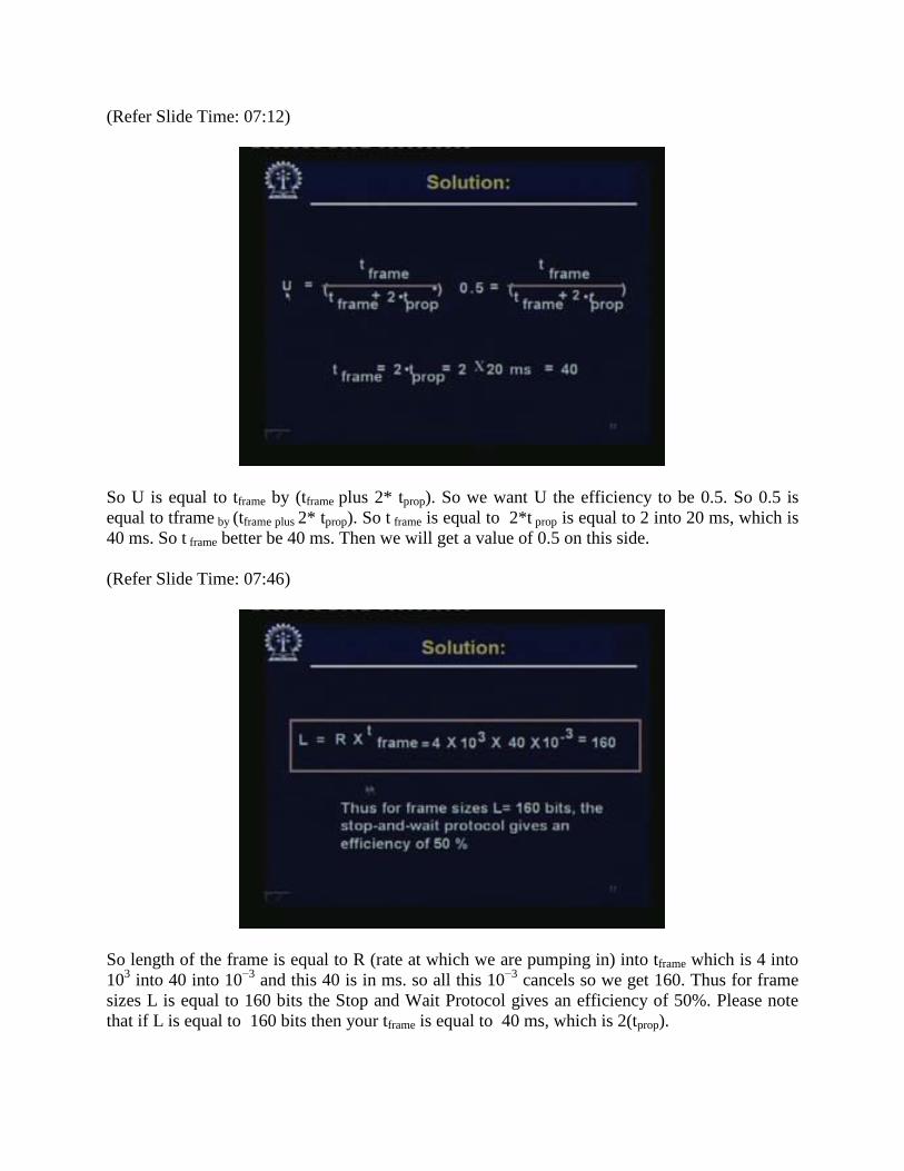
So U is equal to tframe by (tframe plus 2* tprop). So we want U the efficiency to be 0.5. So 0.5 is equal to tframe by (tframe plus 2* tprop). So t frame is equal to 2*t prop is equal to 2 into 20 ms, which is 40 ms. So t frame better be 40 ms. Then we will get a value of 0.5 on this side. (Refer Slide Time: 07:46)

So length of the frame is equal to R (rate at which we are pumping in) into tframe which is 4 into 103 into 40 into 10−3 and this 40 is in ms. so all this 10−3 cancels so we get 160. Thus for frame sizes L is equal to 160 bits the Stop and Wait Protocol gives an efficiency of 50%. Please note that if L is equal to 160 bits then your tframe is equal to 40 ms, which is 2(tprop).


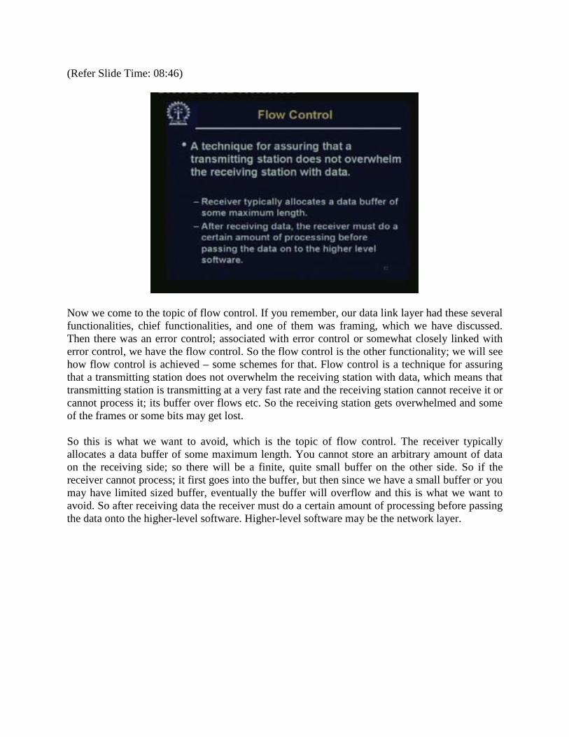
Now we come to the topic of flow control. If you remember, our data link layer had these several functionalities, chief functionalities, and one of them was framing, which we have discussed. Then there was an error control; associated with error control or somewhat closely linked with error control, we have the flow control. So the flow control is the other functionality; we will see how flow control is achieved – some schemes for that. Flow control is a technique for assuring that a transmitting station does not overwhelm the receiving station with data, which means that transmitting station is transmitting at a very fast rate and the receiving station cannot receive it or cannot process it; its buffer over flows etc. So the receiving station gets overwhelmed and some of the frames or some bits may get lost. So this is what we want to avoid, which is the topic of flow control. The receiver typically allocates a data buffer of some maximum length. You cannot store an arbitrary amount of data on the receiving side; so there will be a finite, quite small buffer on the other side. So if the receiver cannot process; it first goes into the buffer, but then since we have a small buffer or you may have limited sized buffer, eventually the buffer will overflow and this is what we want to avoid. So after receiving data the receiver must do a certain amount of processing before passing the data onto the higher-level software. Higher-level software may be the network layer.


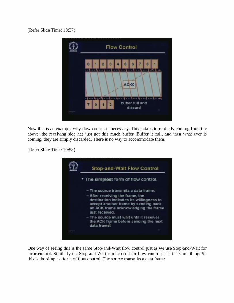
Now this is an example why flow control is necessary. This data is torrentially coming from the above; the receiving side has just got this much buffer. Buffer is full, and then what ever is coming, they are simply discarded. There is no way to accommodate them. (Refer Slide Time: 10:58)

One way of seeing this is the same Stop-and-Wait flow control just as we use Stop-and-Wait for error control. Similarly the Stop-and-Wait can be used for flow control; it is the same thing. So this is the simplest form of flow control. The source transmits a data frame.

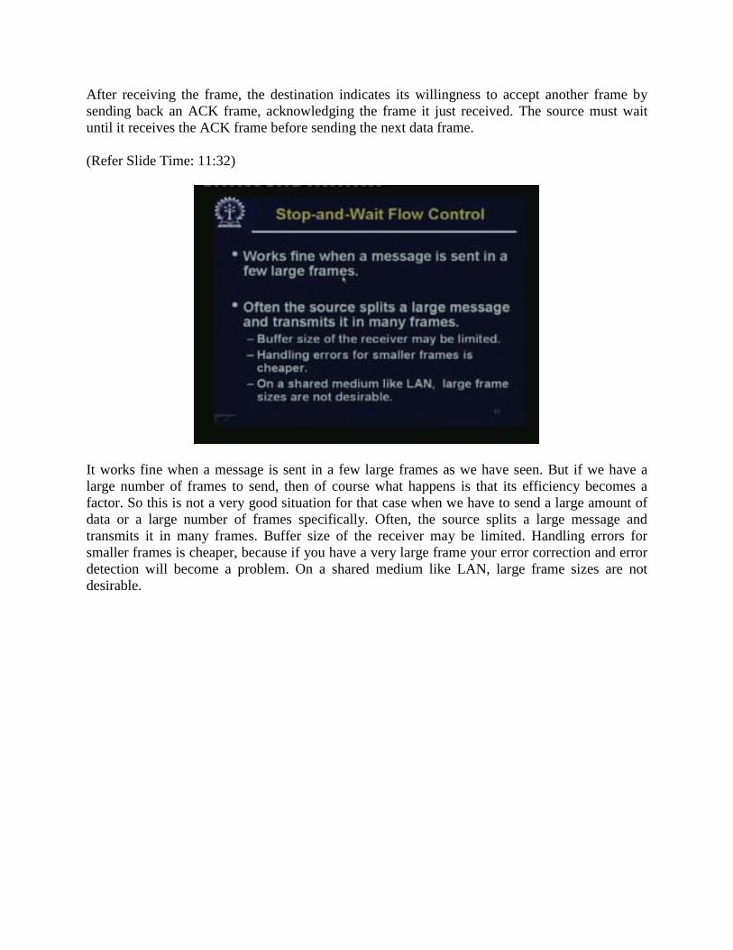
After receiving the frame, the destination indicates its willingness to accept another frame by sending back an ACK frame, acknowledging the frame it just received. The source must wait until it receives the ACK frame before sending the next data frame. (Refer Slide Time: 11:32)

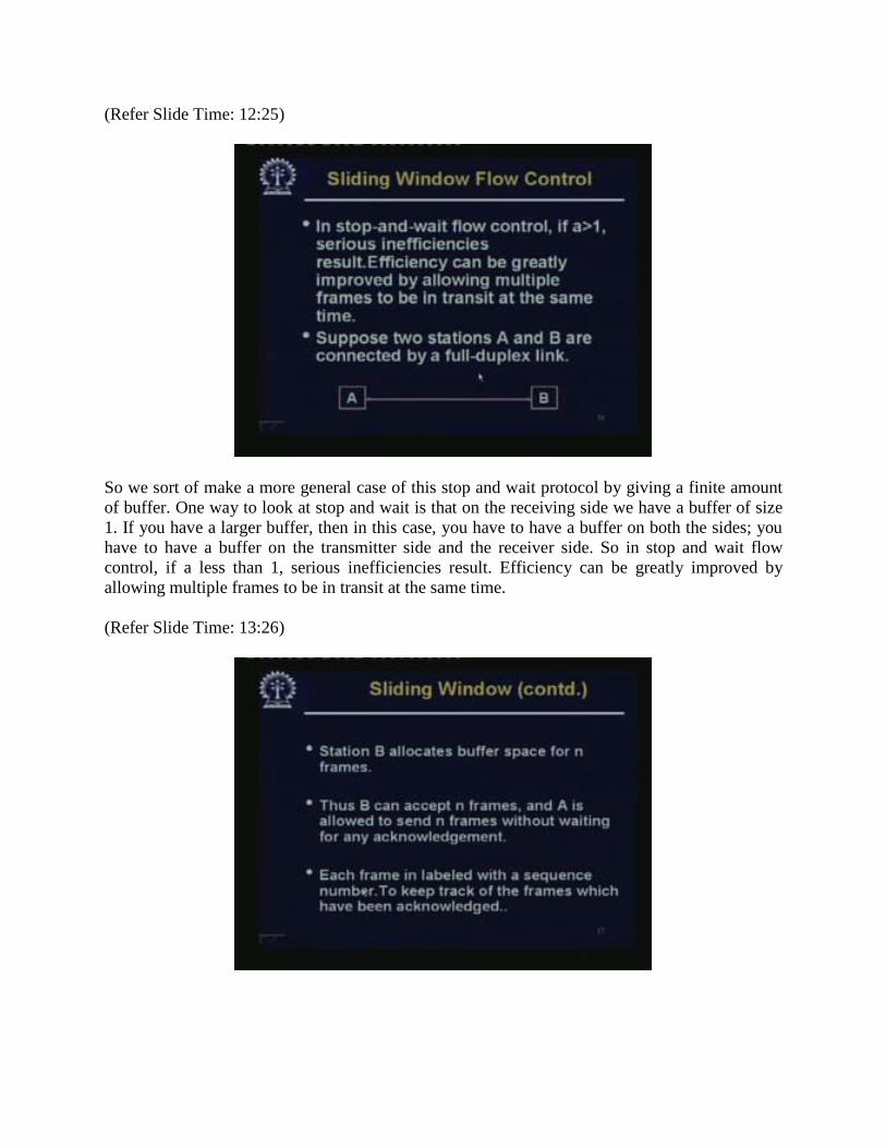
It works fine when a message is sent in a few large frames as we have seen. But if we have a large number of frames to send, then of course what happens is that its efficiency becomes a factor. So this is not a very good situation for that case when we have to send a large amount of data or a large number of frames specifically. Often, the source splits a large message and transmits it in many frames. Buffer size of the receiver may be limited. Handling errors for smaller frames is cheaper, because if you have a very large frame your error correction and error detection will become a problem. On a shared medium like LAN, large frame sizes are not desirable.


So we sort of make a more general case of this stop and wait protocol by giving a finite amount of buffer. One way to look at stop and wait is that on the receiving side we have a buffer of size 1. If you have a larger buffer, then in this case, you have to have a buffer on both the sides; you have to have a buffer on the transmitter side and the receiver side. So in stop and wait flow control, if a less than 1, serious inefficiencies result. Efficiency can be greatly improved by allowing multiple frames to be in transit at the same time. (Refer Slide Time: 13:26)

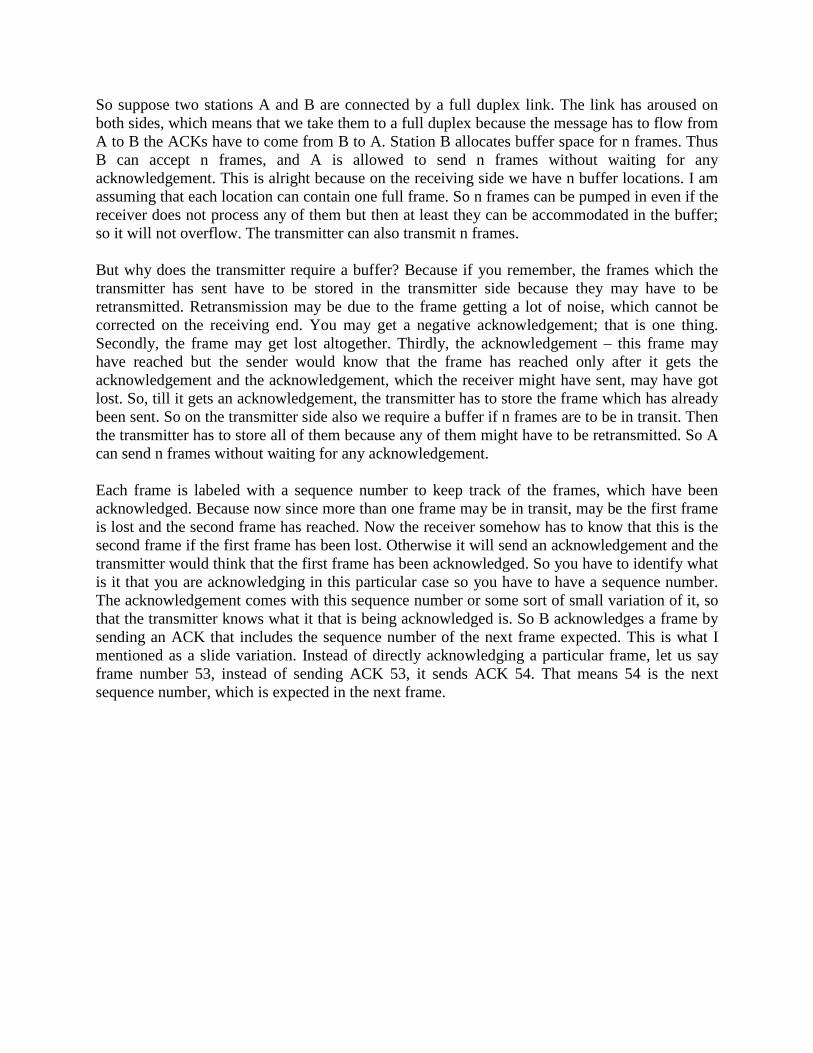
So suppose two stations A and B are connected by a full duplex link. The link has aroused on both sides, which means that we take them to a full duplex because the message has to flow from A to B the ACKs have to come from B to A. Station B allocates buffer space for n frames. Thus B can accept n frames, and A is allowed to send n frames without waiting for any acknowledgement. This is alright because on the receiving side we have n buffer locations. I am assuming that each location can contain one full frame. So n frames can be pumped in even if the receiver does not process any of them but then at least they can be accommodated in the buffer; so it will not overflow. The transmitter can also transmit n frames. But why does the transmitter require a buffer? Because if you remember, the frames which the transmitter has sent have to be stored in the transmitter side because they may have to be retransmitted. Retransmission may be due to the frame getting a lot of noise, which cannot be corrected on the receiving end. You may get a negative acknowledgement; that is one thing. Secondly, the frame may get lost altogether. Thirdly, the acknowledgement – this frame may have reached but the sender would know that the frame has reached only after it gets the acknowledgement and the acknowledgement, which the receiver might have sent, may have got lost. So, till it gets an acknowledgement, the transmitter has to store the frame which has already been sent. So on the transmitter side also we require a buffer if n frames are to be in transit. Then the transmitter has to store all of them because any of them might have to be retransmitted. So A can send n frames without waiting for any acknowledgement. Each frame is labeled with a sequence number to keep track of the frames, which have been acknowledged. Because now since more than one frame may be in transit, may be the first frame is lost and the second frame has reached. Now the receiver somehow has to know that this is the second frame if the first frame has been lost. Otherwise it will send an acknowledgement and the transmitter would think that the first frame has been acknowledged. So you have to identify what is it that you are acknowledging in this particular case so you have to have a sequence number. The acknowledgement comes with this sequence number or some sort of small variation of it, so that the transmitter knows what it that is being acknowledged is. So B acknowledges a frame by sending an ACK that includes the sequence number of the next frame expected. This is what I mentioned as a slide variation. Instead of directly acknowledging a particular frame, let us say frame number 53, instead of sending ACK 53, it sends ACK 54. That means 54 is the next sequence number, which is expected in the next frame.


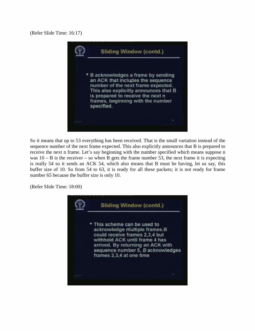
So it means that up to 53 everything has been received. That is the small variation instead of the sequence number of the next frame expected. This also explicitly announces that B is prepared to receive the next n frame. Let’s say beginning with the number specified which means suppose n was 10 – B is the receiver – so when B gets the frame number 53, the next frame it is expecting is really 54 so it sends an ACK 54, which also means that B must be having, let us say, this buffer size of 10. So from 54 to 63, it is ready for all these packets; it is not ready for frame number 65 because the buffer size is only 10. (Refer Slide Time: 18:00)

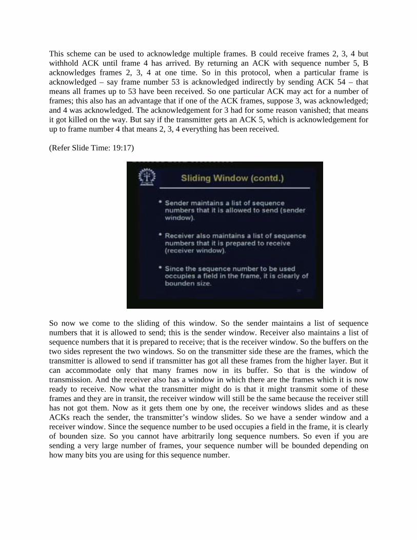
This scheme can be used to acknowledge multiple frames. B could receive frames 2, 3, 4 but withhold ACK until frame 4 has arrived. By returning an ACK with sequence number 5, B acknowledges frames 2, 3, 4 at one time. So in this protocol, when a particular frame is acknowledged – say frame number 53 is acknowledged indirectly by sending ACK 54 – that means all frames up to 53 have been received. So one particular ACK may act for a number of frames; this also has an advantage that if one of the ACK frames, suppose 3, was acknowledged; and 4 was acknowledged. The acknowledgement for 3 had for some reason vanished; that means it got killed on the way. But say if the transmitter gets an ACK 5, which is acknowledgement for up to frame number 4 that means 2, 3, 4 everything has been received. (Refer Slide Time: 19:17)

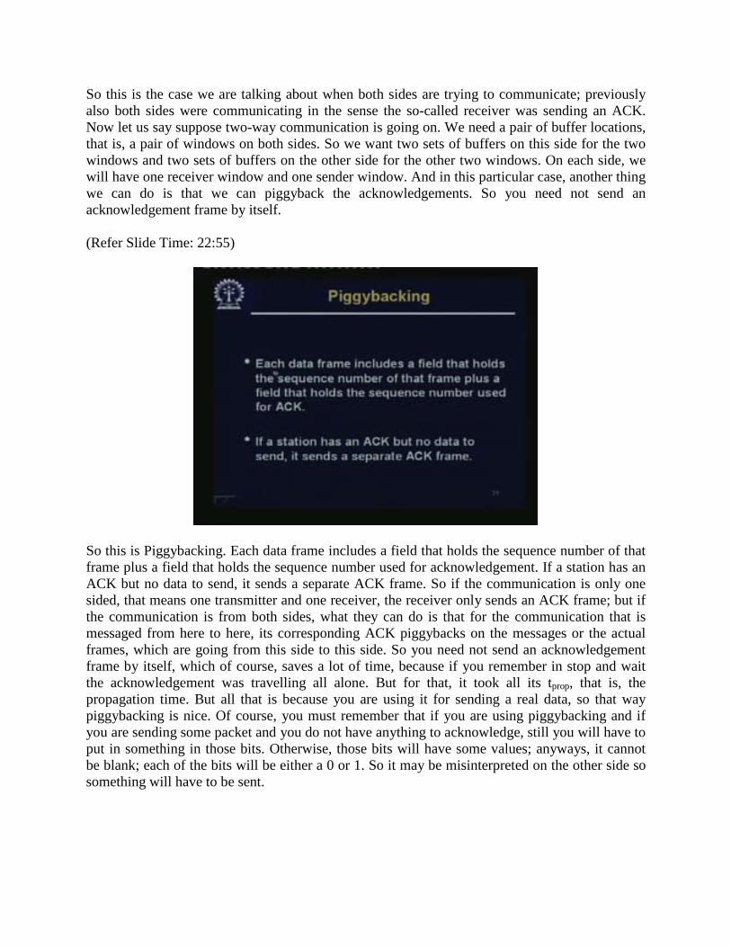
So now we come to the sliding of this window. So the sender maintains a list of sequence numbers that it is allowed to send; this is the sender window. Receiver also maintains a list of sequence numbers that it is prepared to receive; that is the receiver window. So the buffers on the two sides represent the two windows. So on the transmitter side these are the frames, which the transmitter is allowed to send if transmitter has got all these frames from the higher layer. But it can accommodate only that many frames now in its buffer. So that is the window of transmission. And the receiver also has a window in which there are the frames which it is now ready to receive. Now what the transmitter might do is that it might transmit some of these frames and they are in transit, the receiver window will still be the same because the receiver still has not got them. Now as it gets them one by one, the receiver windows slides and as these ACKs reach the sender, the transmitter’s window slides. So we have a sender window and a receiver window. Since the sequence number to be used occupies a field in the frame, it is clearly of bounden size. So you cannot have arbitrarily long sequence numbers. So even if you are sending a very large number of frames, your sequence number will be bounded depending on how many bits you are using for this sequence number.


So for a k bit field, the range of sequence numbers is 0 through 2k−1 and frames are numbered modulo 2k naturally. So now the frame numbers are going to repeat because of this bounded size of k. If k is equal to 3, after sequence number 7 you have to go back to sequence number 0. The next slide shows a depiction of the sliding window for three bit sequence numbers. (Refer Slide Time: 21:44)

The actual window size needs not be the maximum possible size for a given sequence number length; it could be less actually. So for a three-bit sequence number, a window size of 4 can be configured. If two stations exchange data, each needs to maintain two windows. To save communication capacity, a technique called Piggybacking is used.

So this is the case we are talking about when both sides are trying to communicate; previously also both sides were communicating in the sense the so-called receiver was sending an ACK. Now let us say suppose two-way communication is going on. We need a pair of buffer locations, that is, a pair of windows on both sides. So we want two sets of buffers on this side for the two windows and two sets of buffers on the other side for the other two windows. On each side, we will have one receiver window and one sender window. And in this particular case, another thing we can do is that we can piggyback the acknowledgements. So you need not send an acknowledgement frame by itself. (Refer Slide Time: 22:55)

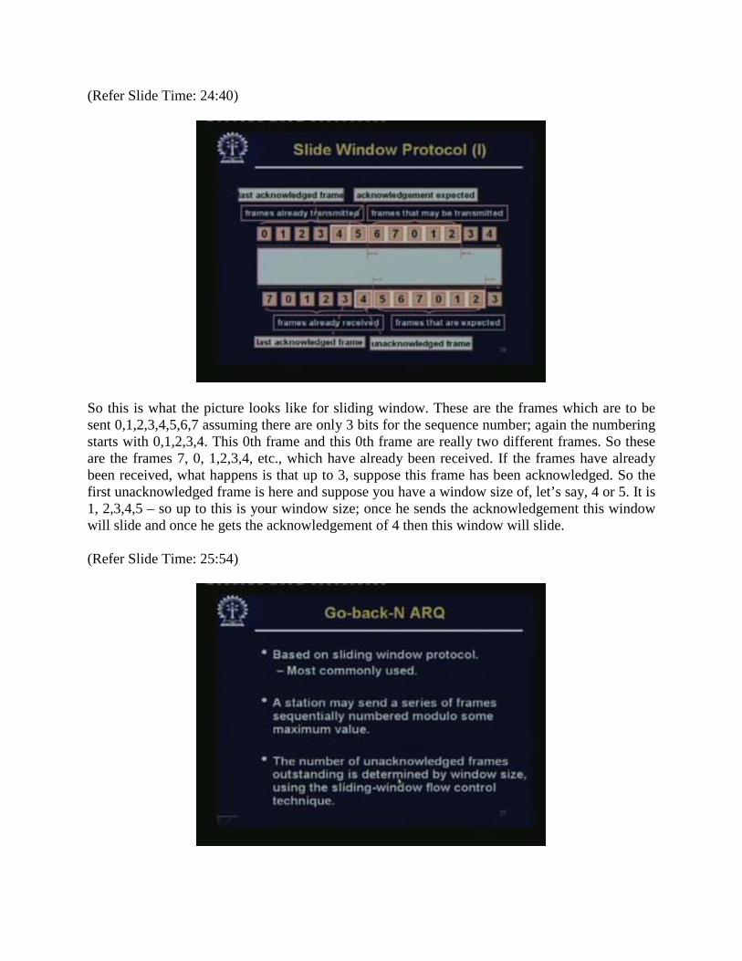
So this is Piggybacking. Each data frame includes a field that holds the sequence number of that frame plus a field that holds the sequence number used for acknowledgement. If a station has an ACK but no data to send, it sends a separate ACK frame. So if the communication is only one sided, that means one transmitter and one receiver, the receiver only sends an ACK frame; but if the communication is from both sides, what they can do is that for the communication that is messaged from here to here, its corresponding ACK piggybacks on the messages or the actual frames, which are going from this side to this side. So you need not send an acknowledgement frame by itself, which of course, saves a lot of time, because if you remember in stop and wait the acknowledgement was travelling all alone. But for that, it took all its tprop, that is, the propagation time. But all that is because you are using it for sending a real data, so that way piggybacking is nice. Of course, you must remember that if you are using piggybacking and if you are sending some packet and you do not have anything to acknowledge, still you will have to put in something in those bits. Otherwise, those bits will have some values; anyways, it cannot be blank; each of the bits will be either a 0 or 1. So it may be misinterpreted on the other side so something will have to be sent.


So this is what the picture looks like for sliding window. These are the frames which are to be sent 0,1,2,3,4,5,6,7 assuming there are only 3 bits for the sequence number; again the numbering starts with 0,1,2,3,4. This 0th frame and this 0th frame are really two different frames. So these are the frames 7, 0, 1,2,3,4, etc., which have already been received. If the frames have already been received, what happens is that up to 3, suppose this frame has been acknowledged. So the first unacknowledged frame is here and suppose you have a window size of, let’s say, 4 or 5. It is 1, 2,3,4,5 – so up to this is your window size; once he sends the acknowledgement this window will slide and once he gets the acknowledgement of 4 then this window will slide. (Refer Slide Time: 25:54)

There are some variations of these acknowledgements we can do; we will discuss that. These variations just try to make it a bit more efficient. We will just look at a couple of variations now. One is Go-back-N ARQ. This is once again based on the same basic sliding window protocol, which is mostly commonly used. A station may send a series of frames sequentially numbered modulo some maximum value as usual. The number of unacknowledged frames outstanding is determined by window size, using the sliding window flow control technique. (Refer Slide Time: 26:41)

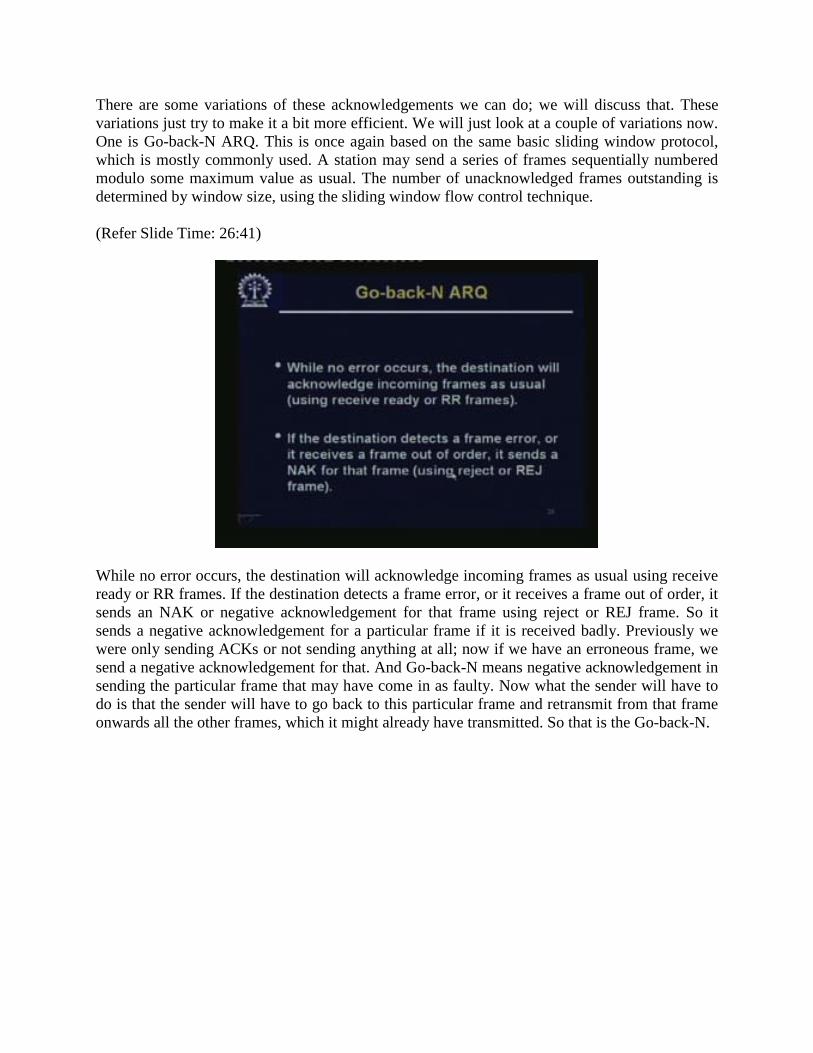
While no error occurs, the destination will acknowledge incoming frames as usual using receive ready or RR frames. If the destination detects a frame error, or it receives a frame out of order, it sends an NAK or negative acknowledgement for that frame using reject or REJ frame. So it sends a negative acknowledgement for a particular frame if it is received badly. Previously we were only sending ACKs or not sending anything at all; now if we have an erroneous frame, we send a negative acknowledgement for that. And Go-back-N means negative acknowledgement in sending the particular frame that may have come in as faulty. Now what the sender will have to do is that the sender will have to go back to this particular frame and retransmit from that frame onwards all the other frames, which it might already have transmitted. So that is the Go-back-N.


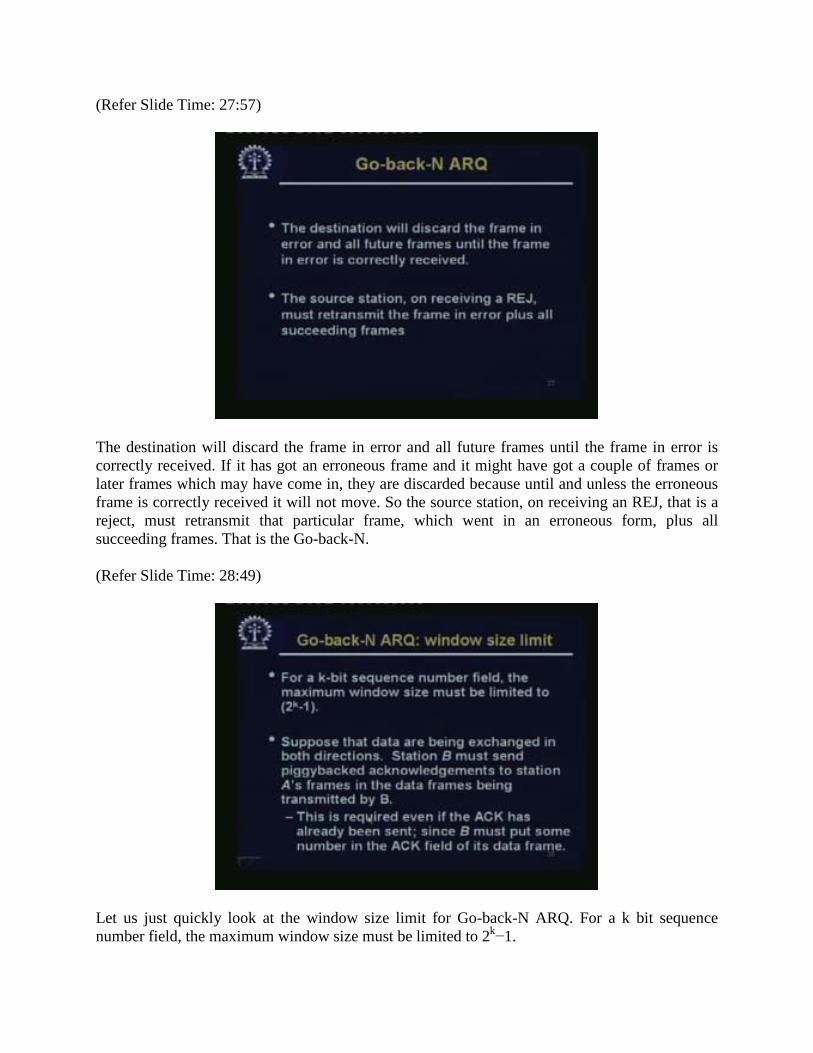
The destination will discard the frame in error and all future frames until the frame in error is correctly received. If it has got an erroneous frame and it might have got a couple of frames or later frames which may have come in, they are discarded because until and unless the erroneous frame is correctly received it will not move. So the source station, on receiving an REJ, that is a reject, must retransmit that particular frame, which went in an erroneous form, plus all succeeding frames. That is the Go-back-N. (Refer Slide Time: 28:49)

Let us just quickly look at the window size limit for Go-back-N ARQ. For a k bit sequence number field, the maximum window size must be limited to 2k−1.

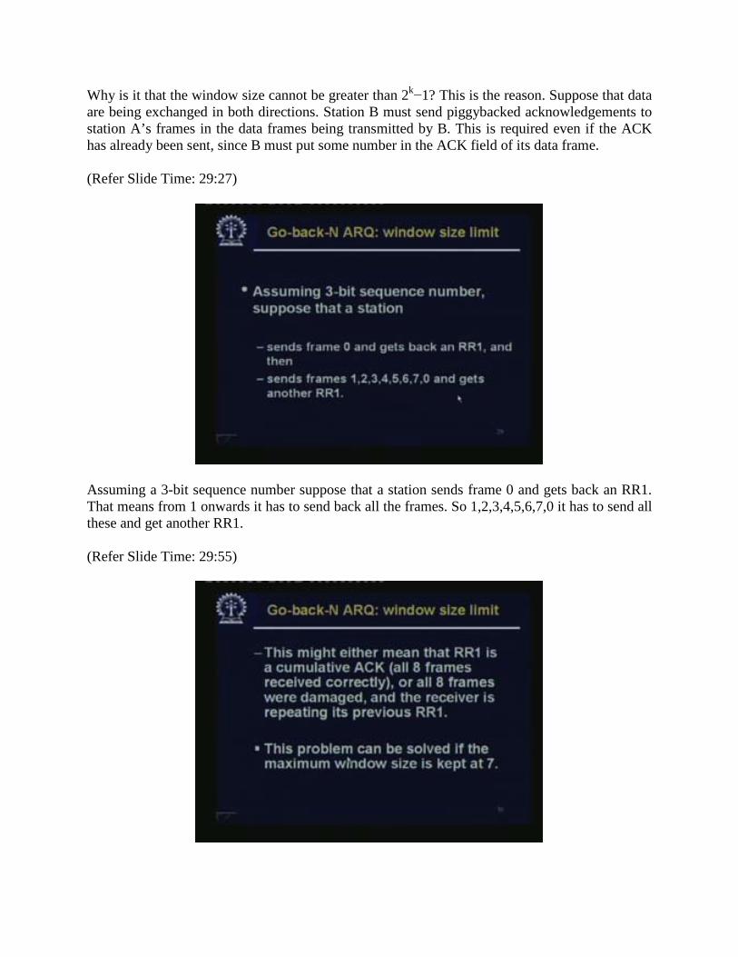
Why is it that the window size cannot be greater than 2k−1? This is the reason. Suppose that data are being exchanged in both directions. Station B must send piggybacked acknowledgements to station A’s frames in the data frames being transmitted by B. This is required even if the ACK has already been sent, since B must put some number in the ACK field of its data frame. (Refer Slide Time: 29:27)

Assuming a 3-bit sequence number suppose that a station sends frame 0 and gets back an RR1. That means from 1 onwards it has to send back all the frames. So 1,2,3,4,5,6,7,0 it has to send all these and get another RR1. (Refer Slide Time: 29:55)

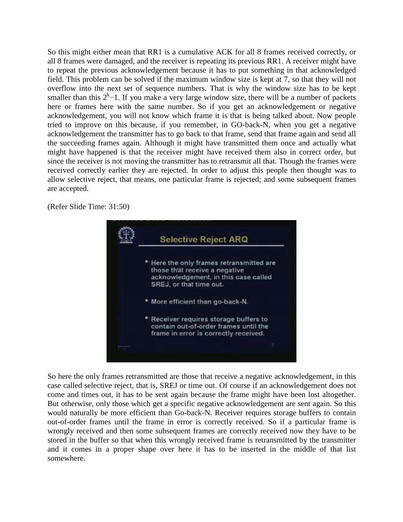
So this might either mean that RR1 is a cumulative ACK for all 8 frames received correctly, or all 8 frames were damaged, and the receiver is repeating its previous RR1. A receiver might have to repeat the previous acknowledgement because it has to put something in that acknowledged field. This problem can be solved if the maximum window size is kept at 7, so that they will not overflow into the next set of sequence numbers. That is why the window size has to be kept smaller than this 2k−1. If you make a very large window size, there will be a number of packets here or frames here with the same number. So if you get an acknowledgement or negative acknowledgement, you will not know which frame it is that is being talked about. Now people tried to improve on this because, if you remember, in GO-back-N, when you get a negative acknowledgement the transmitter has to go back to that frame, send that frame again and send all the succeeding frames again. Although it might have transmitted them once and actually what might have happened is that the receiver might have received them also in correct order, but since the receiver is not moving the transmitter has to retransmit all that. Though the frames were received correctly earlier they are rejected. In order to adjust this people then thought was to allow selective reject, that means, one particular frame is rejected; and some subsequent frames are accepted. (Refer Slide Time: 31:50)

So here the only frames retransmitted are those that receive a negative acknowledgement, in this case called selective reject, that is, SREJ or time out. Of course if an acknowledgement does not come and times out, it has to be sent again because the frame might have been lost altogether. But otherwise, only those which get a specific negative acknowledgement are sent again. So this would naturally be more efficient than Go-back-N. Receiver requires storage buffers to contain out-of-order frames until the frame in error is correctly received. So if a particular frame is wrongly received and then some subsequent frames are correctly received now they have to be stored in the buffer so that when this wrongly received frame is retransmitted by the transmitter and it comes in a proper shape over here it has to be inserted in the middle of that list somewhere.


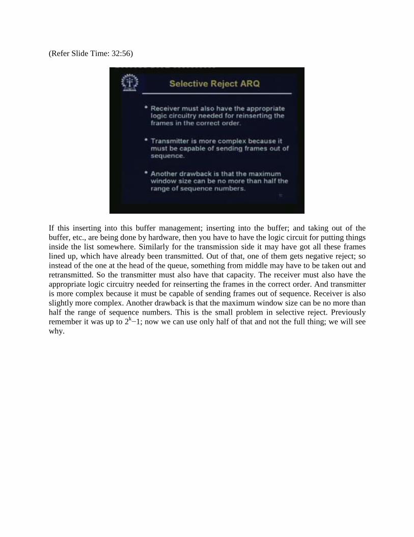
If this inserting into this buffer management; inserting into the buffer; and taking out of the buffer, etc., are being done by hardware, then you have to have the logic circuit for putting things inside the list somewhere. Similarly for the transmission side it may have got all these frames lined up, which have already been transmitted. Out of that, one of them gets negative reject; so instead of the one at the head of the queue, something from middle may have to be taken out and retransmitted. So the transmitter must also have that capacity. The receiver must also have the appropriate logic circuitry needed for reinserting the frames in the correct order. And transmitter is more complex because it must be capable of sending frames out of sequence. Receiver is also slightly more complex. Another drawback is that the maximum window size can be no more than half the range of sequence numbers. This is the small problem in selective reject. Previously remember it was up to 2k−1; now we can use only half of that and not the full thing; we will see why.


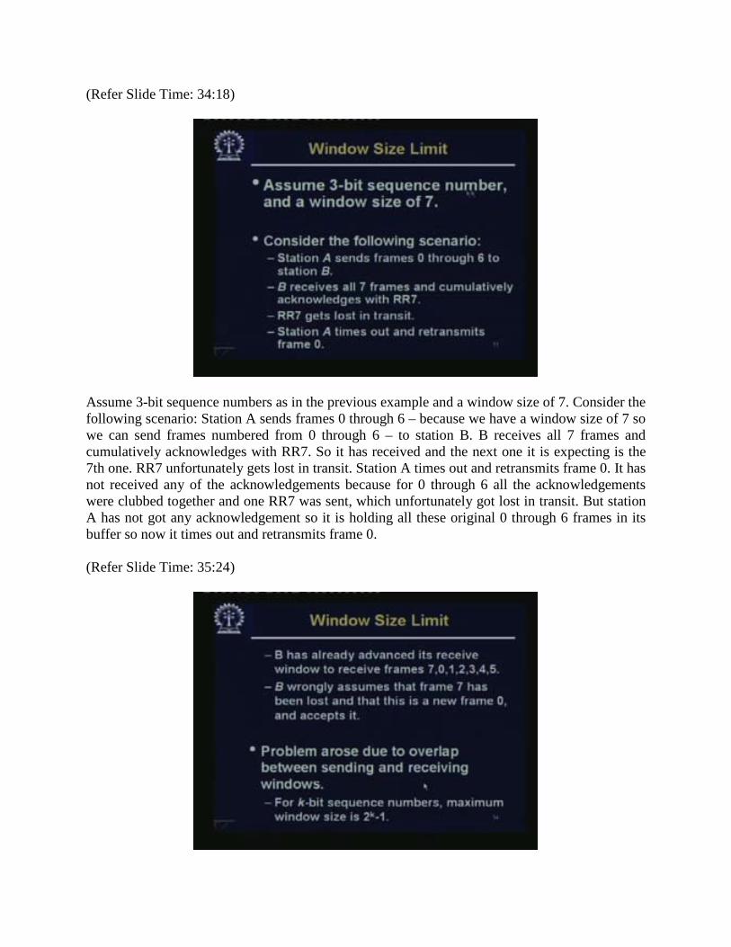
Assume 3-bit sequence numbers as in the previous example and a window size of 7. Consider the following scenario: Station A sends frames 0 through 6 – because we have a window size of 7 so we can send frames numbered from 0 through 6 – to station B. B receives all 7 frames and cumulatively acknowledges with RR7. So it has received and the next one it is expecting is the 7th one. RR7 unfortunately gets lost in transit. Station A times out and retransmits frame 0. It has not received any of the acknowledgements because for 0 through 6 all the acknowledgements were clubbed together and one RR7 was sent, which unfortunately got lost in transit. But station A has not got any acknowledgement so it is holding all these original 0 through 6 frames in its buffer so now it times out and retransmits frame 0. (Refer Slide Time: 35:24)

B has already advanced its received window to receive frames 7, 0, 1, 2, 3, 4, 5. Now B wrongly assumes that frame 7 has been lost and that this is the new frame 0, and accepts it. So this old frame 0 is interpreted as the new 0 number frame by B and it assumes that 7 has been lost in transit so may be later on a negative acknowledgement or selective reject for 7 would be sent. But this 0 frame now has gone out of order. So the problem arose due to overlap between sending and receiving windows. For k bit sequence numbers, maximum window size therefore has to be smaller. (Refer Slide Time: 36:18)

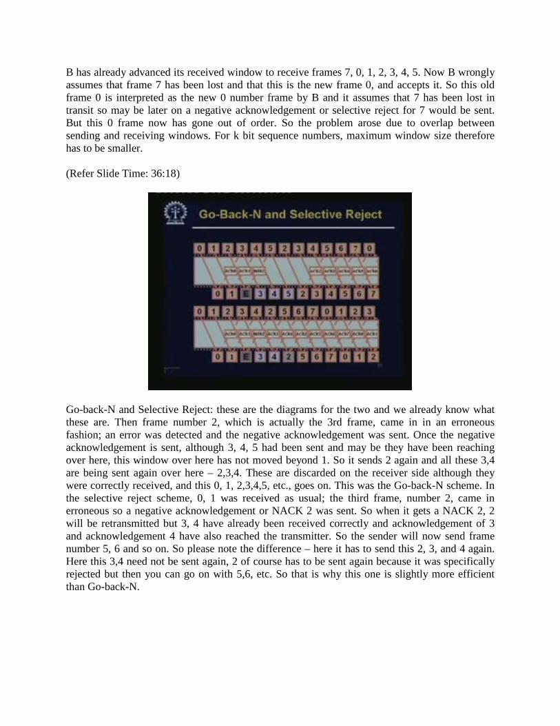
Go-back-N and Selective Reject: these are the diagrams for the two and we already know what these are. Then frame number 2, which is actually the 3rd frame, came in in an erroneous fashion; an error was detected and the negative acknowledgement was sent. Once the negative acknowledgement is sent, although 3, 4, 5 had been sent and may be they have been reaching over here, this window over here has not moved beyond 1. So it sends 2 again and all these 3,4 are being sent again over here – 2,3,4. These are discarded on the receiver side although they were correctly received, and this 0, 1, 2,3,4,5, etc., goes on. This was the Go-back-N scheme. In the selective reject scheme, 0, 1 was received as usual; the third frame, number 2, came in erroneous so a negative acknowledgement or NACK 2 was sent. So when it gets a NACK 2, 2 will be retransmitted but 3, 4 have already been received correctly and acknowledgement of 3 and acknowledgement 4 have also reached the transmitter. So the sender will now send frame number 5, 6 and so on. So please note the difference – here it has to send this 2, 3, and 4 again. Here this 3,4 need not be sent again, 2 of course has to be sent again because it was specifically rejected but then you can go on with 5,6, etc. So that is why this one is slightly more efficient than Go-back-N.


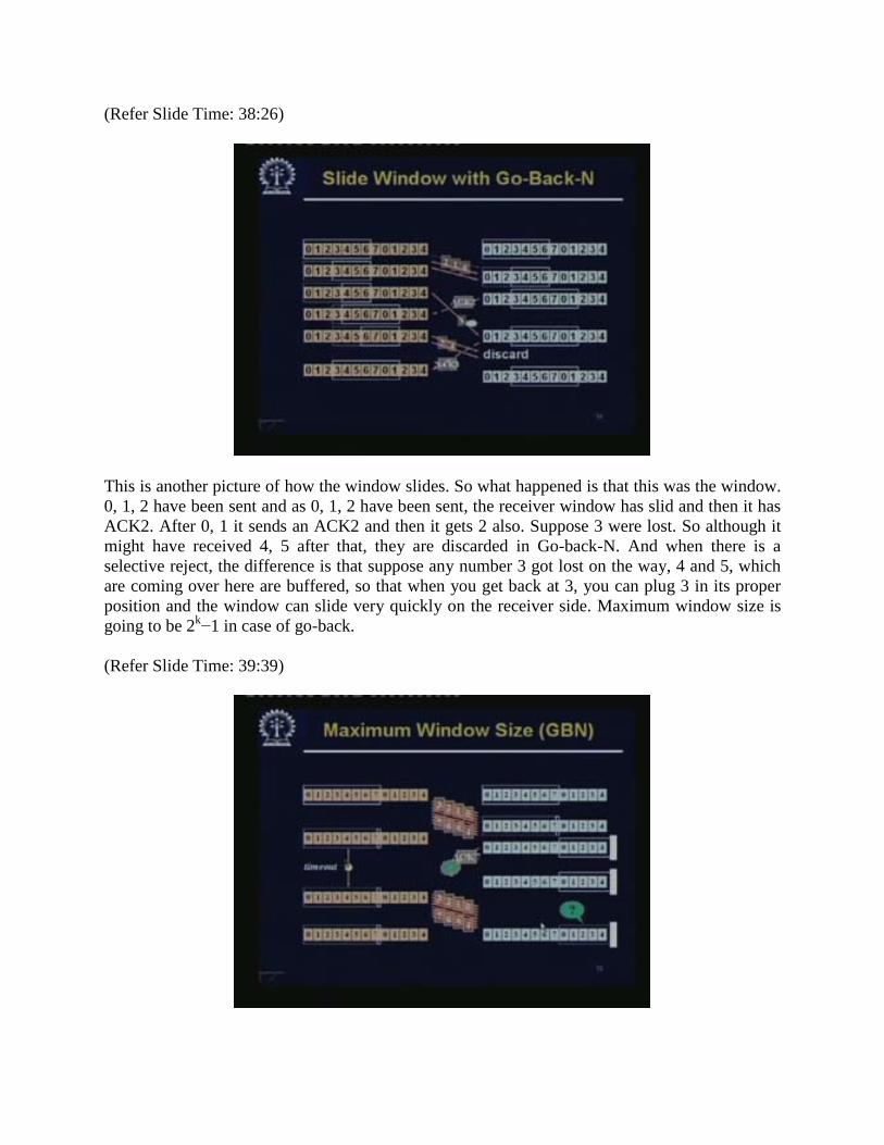
This is another picture of how the window slides. So what happened is that this was the window. 0, 1, 2 have been sent and as 0, 1, 2 have been sent, the receiver window has slid and then it has ACK2. After 0, 1 it sends an ACK2 and then it gets 2 also. Suppose 3 were lost. So although it might have received 4, 5 after that, they are discarded in Go-back-N. And when there is a selective reject, the difference is that suppose any number 3 got lost on the way, 4 and 5, which are coming over here are buffered, so that when you get back at 3, you can plug 3 in its proper position and the window can slide very quickly on the receiver side. Maximum window size is going to be 2k−1 in case of go-back. (Refer Slide Time: 39:39)


We have discussed some of the major techniques, which are used in data link layer. What we will do now is that we will look at just one more protocol. This is a somewhat general version. We have already discussed PPP, that is, point-to point protocol, which is used for just point-to-point communication. But there could be a point-to-multi-point communication also; for this we have this high level data link control. This is the name of the protocol, or HDLC in short. This is not considered so high level any longer; but this is an important protocol. So there are some variations of this which are used in various places. (Refer Slide Time: 41:01)

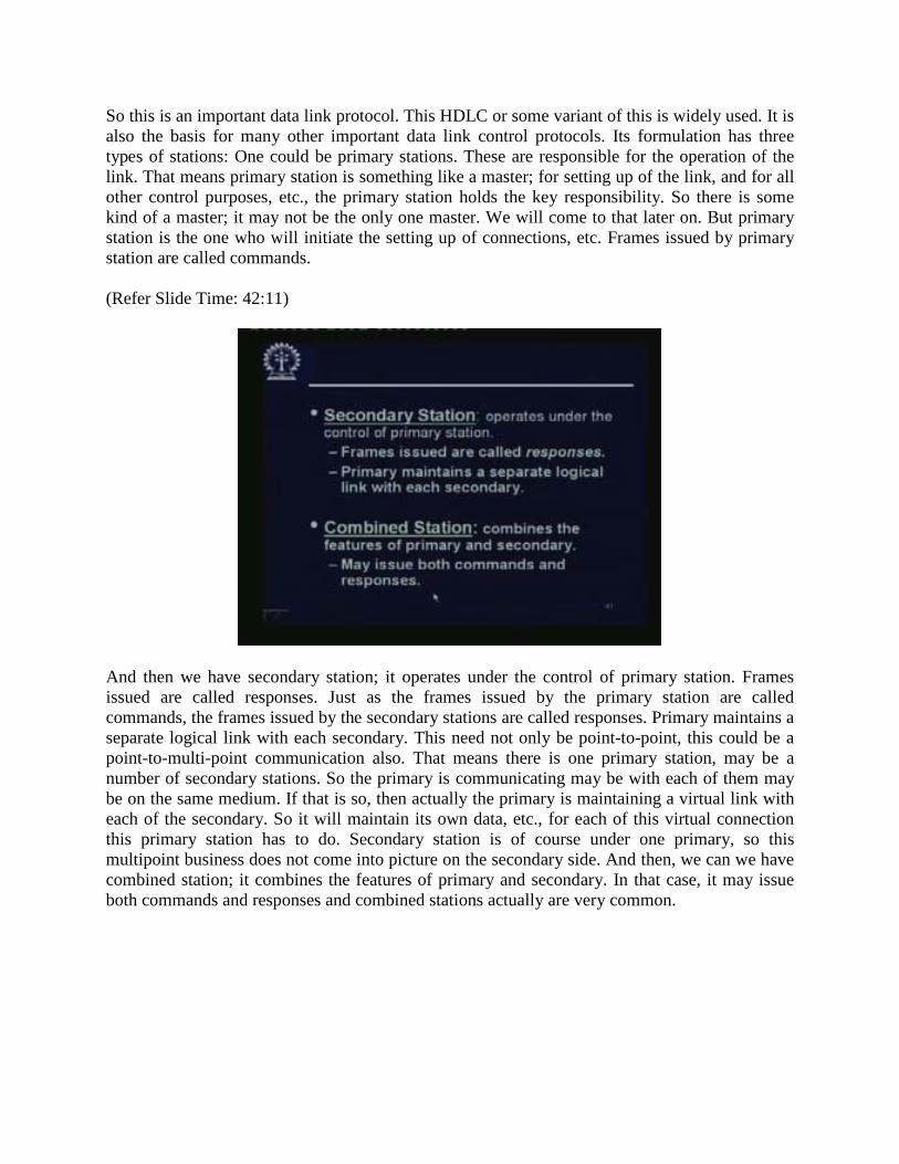
So this is an important data link protocol. This HDLC or some variant of this is widely used. It is also the basis for many other important data link control protocols. Its formulation has three types of stations: One could be primary stations. These are responsible for the operation of the link. That means primary station is something like a master; for setting up of the link, and for all other control purposes, etc., the primary station holds the key responsibility. So there is some kind of a master; it may not be the only one master. We will come to that later on. But primary station is the one who will initiate the setting up of connections, etc. Frames issued by primary station are called commands. (Refer Slide Time: 42:11)

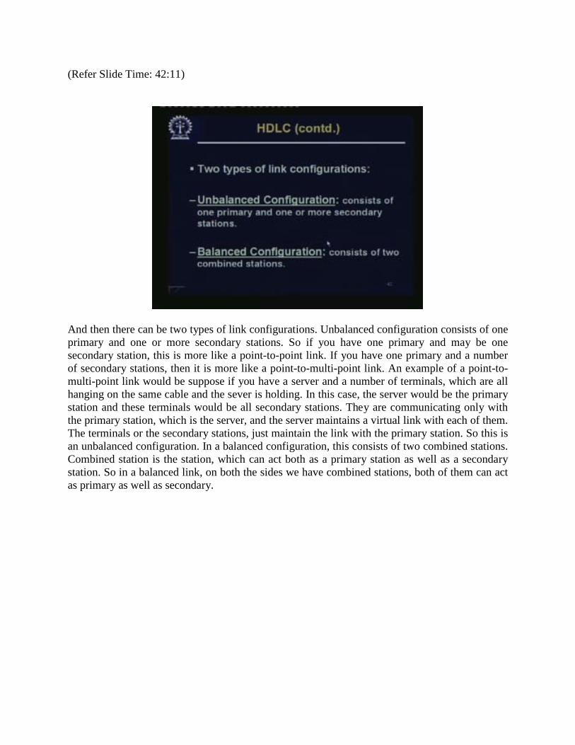
And then we have secondary station; it operates under the control of primary station. Frames issued are called responses. Just as the frames issued by the primary station are called commands, the frames issued by the secondary stations are called responses. Primary maintains a separate logical link with each secondary. This need not only be point-to-point, this could be a point-to-multi-point communication also. That means there is one primary station, may be a number of secondary stations. So the primary is communicating may be with each of them may be on the same medium. If that is so, then actually the primary is maintaining a virtual link with each of the secondary. So it will maintain its own data, etc., for each of this virtual connection this primary station has to do. Secondary station is of course under one primary, so this multipoint business does not come into picture on the secondary side. And then, we can we have combined station; it combines the features of primary and secondary. In that case, it may issue both commands and responses and combined stations actually are very common.


And then there can be two types of link configurations. Unbalanced configuration consists of one primary and one or more secondary stations. So if you have one primary and may be one secondary station, this is more like a point-to-point link. If you have one primary and a number of secondary stations, then it is more like a point-to-multi-point link. An example of a point-to-multi-point link would be suppose if you have a server and a number of terminals, which are all hanging on the same cable and the sever is holding. In this case, the server would be the primary station and these terminals would be all secondary stations. They are communicating only with the primary station, which is the server, and the server maintains a virtual link with each of them. The terminals or the secondary stations, just maintain the link with the primary station. So this is an unbalanced configuration. In a balanced configuration, this consists of two combined stations. Combined station is the station, which can act both as a primary station as well as a secondary station. So in a balanced link, on both the sides we have combined stations, both of them can act as primary as well as secondary.


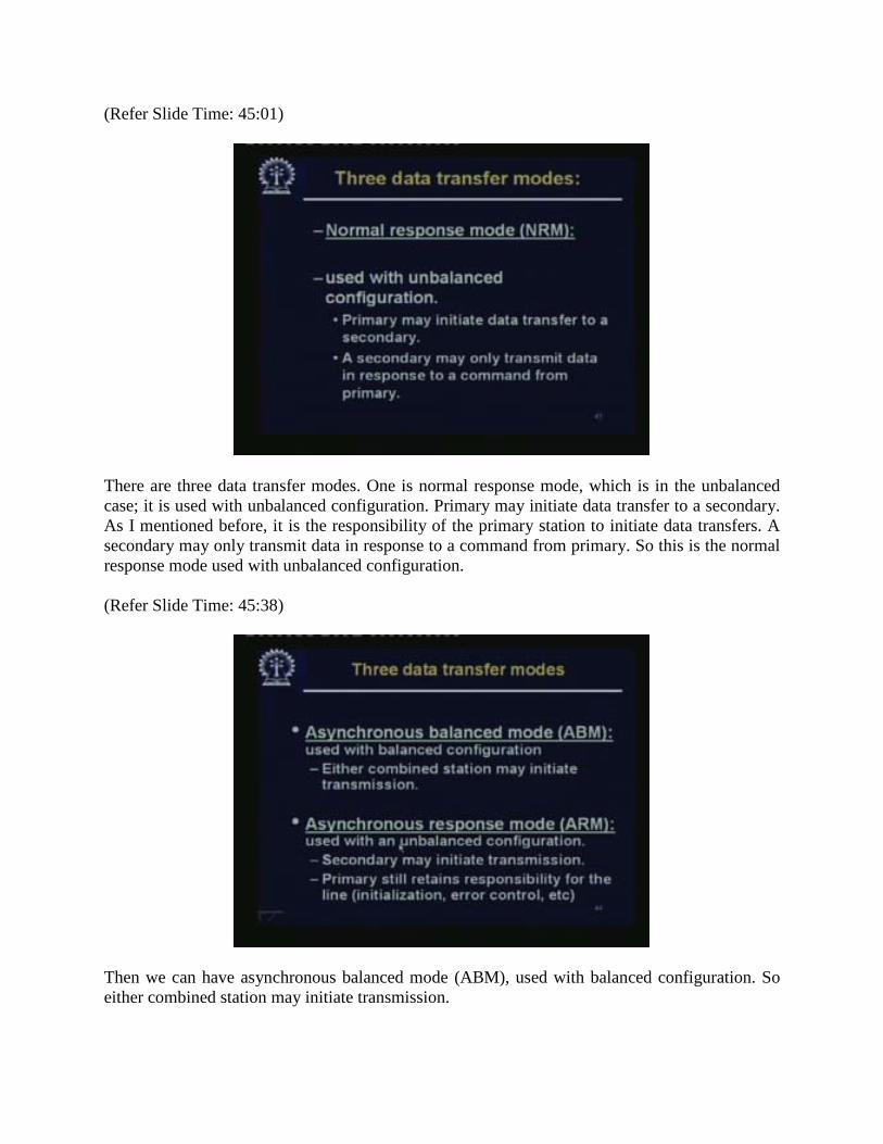
There are three data transfer modes. One is normal response mode, which is in the unbalanced case; it is used with unbalanced configuration. Primary may initiate data transfer to a secondary. As I mentioned before, it is the responsibility of the primary station to initiate data transfers. A secondary may only transmit data in response to a command from primary. So this is the normal response mode used with unbalanced configuration. (Refer Slide Time: 45:38)

Then we can have asynchronous balanced mode (ABM), used with balanced configuration. So either combined station may initiate transmission.

In this case, since it is on the balanced configuration, which means, on both sides of the link we have the two combined stations, both of them can act as primary and secondary and since both of them are combined stations, any of them can initiate the transmission and the transmission can start – this is ABM. And the other is ARM asynchronous response mode used with unbalanced configuration. Here the secondary may initiate transmission. Primary still retains responsibility for the line (initialization, error control etc.) that is done by the primary ARM. This is not very common. (Refer Slide Time: 46:36)

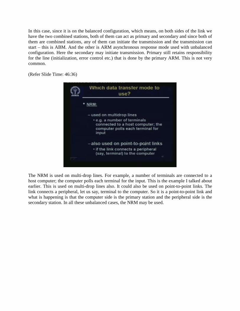
The NRM is used on multi-drop lines. For example, a number of terminals are connected to a host computer; the computer polls each terminal for the input. This is the example I talked about earlier. This is used on multi-drop lines also. It could also be used on point-to-point links. The link connects a peripheral, let us say, terminal to the computer. So it is a point-to-point link and what is happening is that the computer side is the primary station and the peripheral side is the secondary station. In all these unbalanced cases, the NRM may be used.


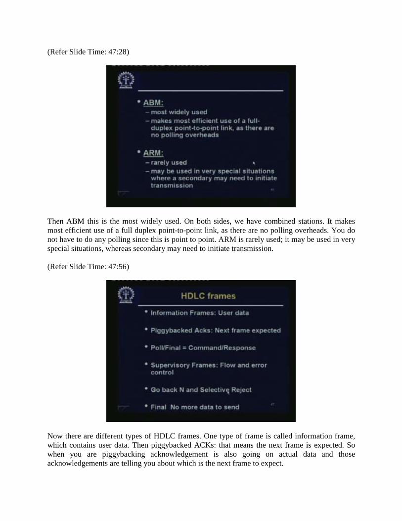
Then ABM this is the most widely used. On both sides, we have combined stations. It makes most efficient use of a full duplex point-to-point link, as there are no polling overheads. You do not have to do any polling since this is point to point. ARM is rarely used; it may be used in very special situations, whereas secondary may need to initiate transmission. (Refer Slide Time: 47:56)

Now there are different types of HDLC frames. One type of frame is called information frame, which contains user data. Then piggybacked ACKs: that means the next frame is expected. So when you are piggybacking acknowledgement is also going on actual data and those acknowledgements are telling you about which is the next frame to expect.

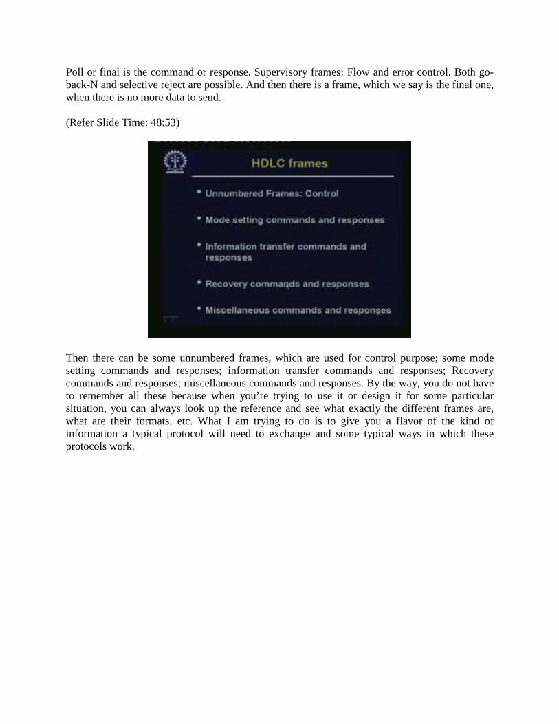
Poll or final is the command or response. Supervisory frames: Flow and error control. Both go-back-N and selective reject are possible. And then there is a frame, which we say is the final one, when there is no more data to send. (Refer Slide Time: 48:53)

Then there can be some unnumbered frames, which are used for control purpose; some mode setting commands and responses; information transfer commands and responses; Recovery commands and responses; miscellaneous commands and responses. By the way, you do not have to remember all these because when you’re trying to use it or design it for some particular situation, you can always look up the reference and see what exactly the different frames are, what are their formats, etc. What I am trying to do is to give you a flavor of the kind of information a typical protocol will need to exchange and some typical ways in which these protocols work.


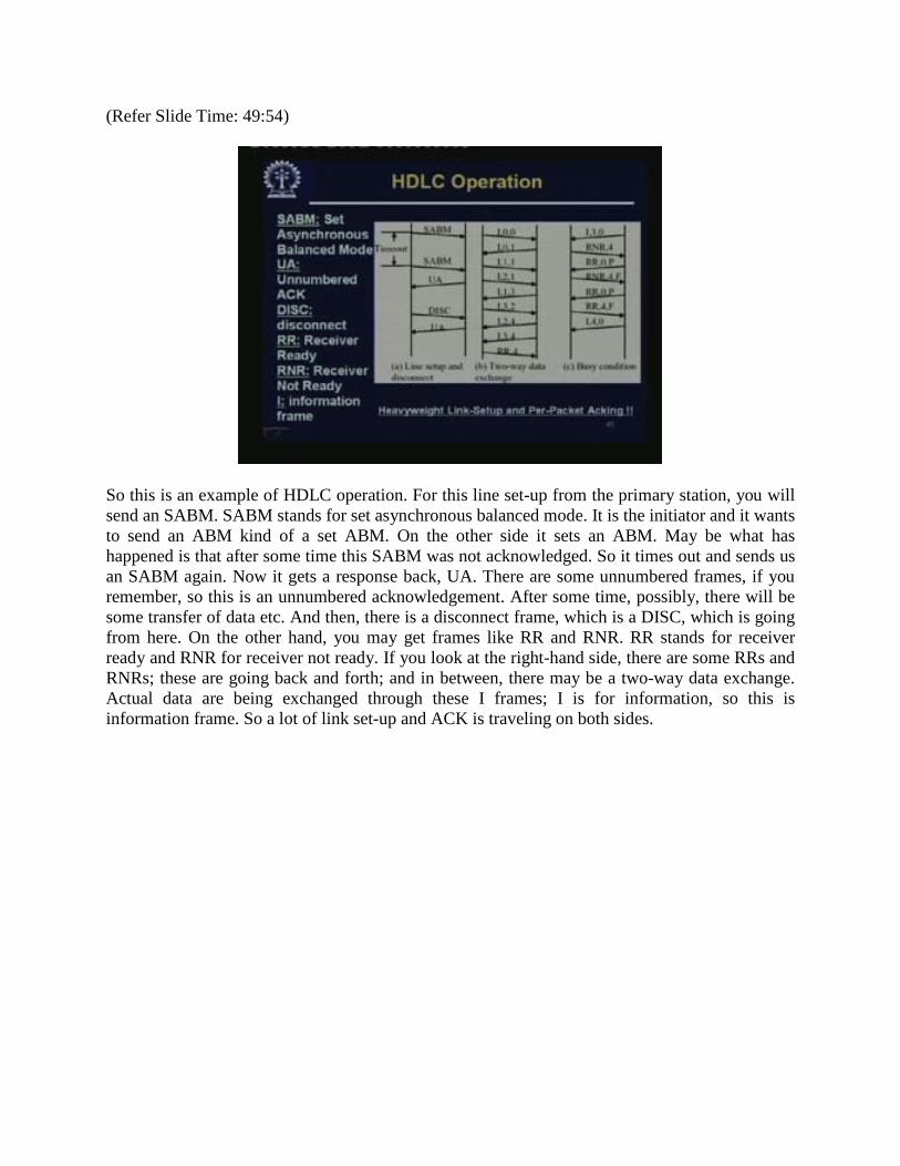
So this is an example of HDLC operation. For this line set-up from the primary station, you will send an SABM. SABM stands for set asynchronous balanced mode. It is the initiator and it wants to send an ABM kind of a set ABM. On the other side it sets an ABM. May be what has happened is that after some time this SABM was not acknowledged. So it times out and sends us an SABM again. Now it gets a response back, UA. There are some unnumbered frames, if you remember, so this is an unnumbered acknowledgement. After some time, possibly, there will be some transfer of data etc. And then, there is a disconnect frame, which is a DISC, which is going from here. On the other hand, you may get frames like RR and RNR. RR stands for receiver ready and RNR for receiver not ready. If you look at the right-hand side, there are some RRs and RNRs; these are going back and forth; and in between, there may be a two-way data exchange. Actual data are being exchanged through these I frames; I is for information, so this is information frame. So a lot of link set-up and ACK is traveling on both sides.


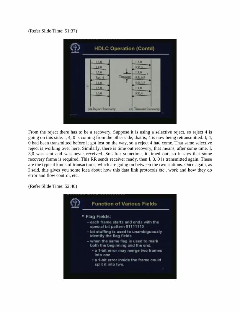
From the reject there has to be a recovery. Suppose it is using a selective reject, so reject 4 is going on this side. I, 4, 0 is coming from the other side; that is, 4 is now being retransmitted. I, 4, 0 had been transmitted before it got lost on the way, so a reject 4 had come. That same selective reject is working over here. Similarly, there is time out recovery; that means, after some time, I, 3,0 was sent and was never received. So after sometime, it timed out; so it says that some recovery frame is required. This RR sends receiver ready, then I, 3, 0 is transmitted again. These are the typical kinds of transactions, which are going on between the two stations. Once again, as I said, this gives you some idea about how this data link protocols etc., work and how they do error and flow control, etc. (Refer Slide Time: 52:48)

We will now take just a quick look at the various fields. There are some flag fields. Each frame starts and ends with the special bit pattern. Of course, if you use a special pattern, in order to accommodate this pattern within the data itself, bit stuffing is used to unambiguously identify the flag fields. Bit stuffing this is not 100% reliable. You must remember when the same flag is used to mark both the beginning and the end; a 1-bit error may merge two frames into one. A 1-bit error in the ending patterns will not be interpreted as an end of frame pattern by the receiving side; so the two frames may get merged. Similarly, a 1-bit error inside the frame could split it into two. This is not 100% correct, but bit stuffing would work most of the time. (Refer Slide Time: 53:55)

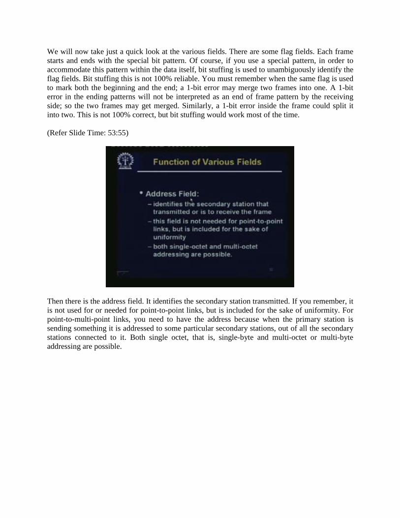
Then there is the address field. It identifies the secondary station transmitted. If you remember, it is not used for or needed for point-to-point links, but is included for the sake of uniformity. For point-to-multi-point links, you need to have the address because when the primary station is sending something it is addressed to some particular secondary stations, out of all the secondary stations connected to it. Both single octet, that is, single-byte and multi-octet or multi-byte addressing are possible.


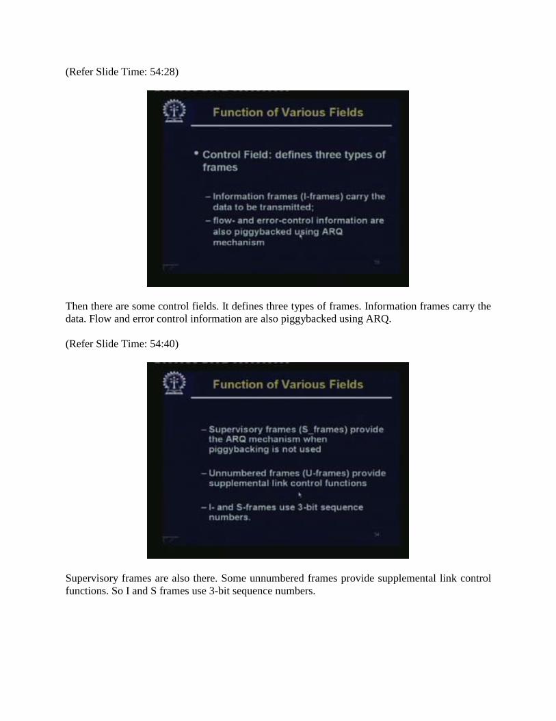
Then there are some control fields. It defines three types of frames. Information frames carry the data. Flow and error control information are also piggybacked using ARQ. (Refer Slide Time: 54:40)

Supervisory frames are also there. Some unnumbered frames provide supplemental link control functions. So I and S frames use 3-bit sequence numbers.


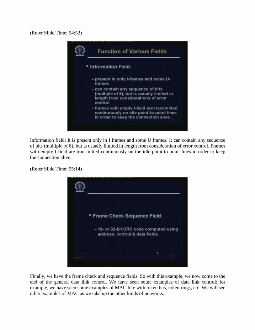
Information field: It is present only in I frames and some U frames. It can contain any sequence of bits (multiple of 8), but is usually limited in length from consideration of error control. Frames with empty I field are transmitted continuously on the idle point-to-point lines in order to keep the connection alive. (Refer Slide Time: 55:14)

Finally, we have the frame check and sequence fields. So with this example, we now come to the end of the general data link control. We have seen some examples of data link control; for example, we have seen some examples of MAC like with token bus, token rings, etc. We will see other examples of MAC as we take up the other kinds of networks.

Similarly, we have seen some kinds of error and data control. A similar approach is used in some other higher layers also. We will talk about it when we come to it and we will talk about some more specific and more widely used systems from the next class onwards. So in the next class, what we will do is that we will look at another type of communication and how MAC is done on that in satellite communication. So, that will be the next topic. Thank you.

Documents

Computer Networks Prof. Sujoy Ghosh Department of …textofvideo.nptel.ac.in/106105081/lec17.pdf · Now let us look at link utilization in Stop and Wait – how much we are utilizing