Fluent 6.2 Software Capabilities - Freevincent.chapin.free.fr/Cours CFD/Doc/Fluent-v6.2-lect_all.pdf · Fluent 6.2 applications: zExternal/internal automotive flows and in-cylinder

Fluent 6.2 Software Capabilities

Basic Training Course

© Fluent Inc. 4/8/2005- 1 -

Introductory FLUENT NotesFLUENT v6.2 Mar 2005

Fluent User Services Center

www.fluentusers.com

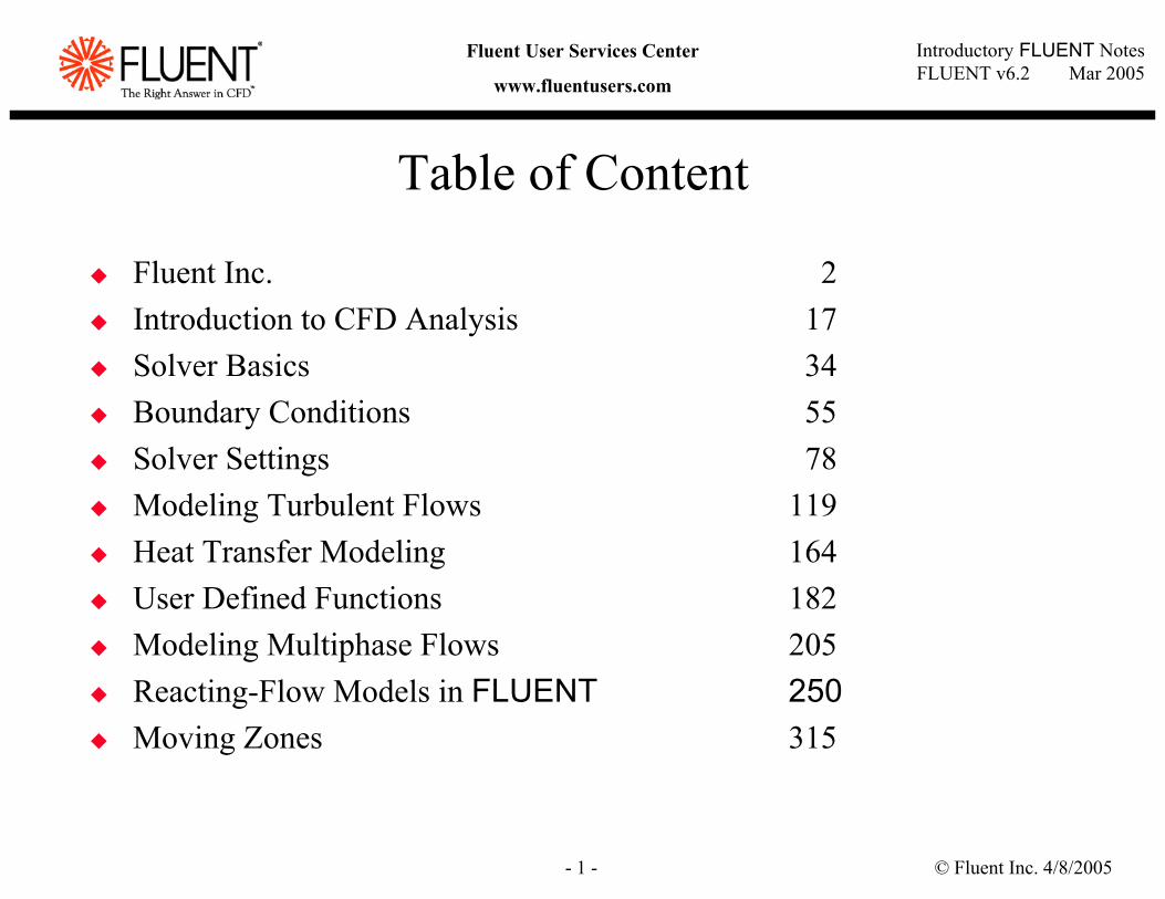
Table of Content

Fluent Inc. 2Introduction to CFD Analysis 17Solver Basics 34Boundary Conditions 55Solver Settings 78Modeling Turbulent Flows 119Heat Transfer Modeling 164User Defined Functions 182Modeling Multiphase Flows 205Reacting-Flow Models in FLUENT 250Moving Zones 315

© Fluent Inc. 4/8/2005- 2 -



www.fluentusers.com

Fluent Inc.

© Fluent Inc. 4/8/2005- 3 -



www.fluentusers.com


www.fluentusers.comPlease register today!Services Include

Release InformationDownload UpdatesDocumentationSupported PlatformsDefects/WorkaroundsPresentationsTrainingOnline Technical Support

Quick Reference GuideOverview and Demo via web based training http://www.fluentusers.com/

© Fluent Inc. 4/8/2005- 4 -



www.fluentusers.com

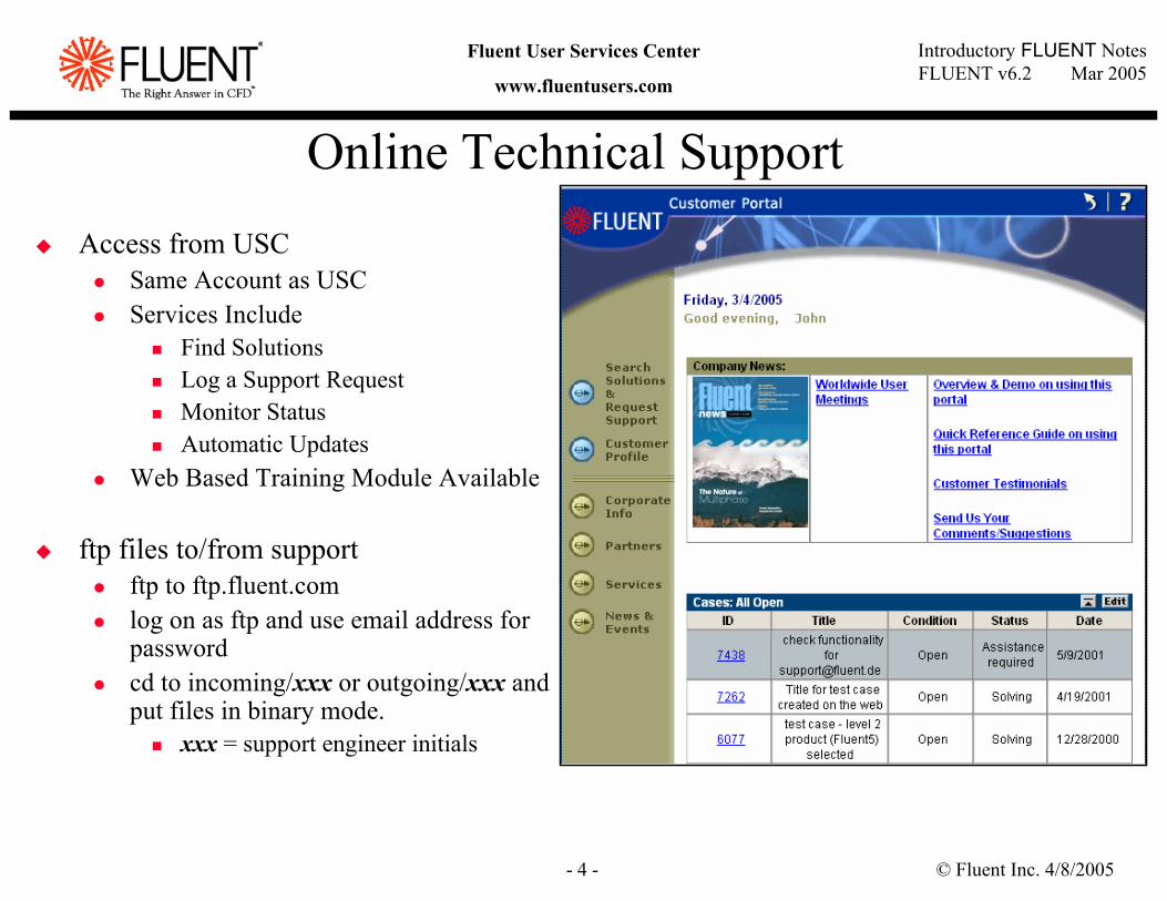
Online Technical SupportAccess from USC

Same Account as USCServices Include

Find SolutionsLog a Support RequestMonitor StatusAutomatic Updates

Web Based Training Module Available

ftp files to/from supportftp to ftp.fluent.comlog on as ftp and use email address for passwordcd to incoming/xxx or outgoing/xxx and put files in binary mode.

xxx = support engineer initials

© Fluent Inc. 4/8/2005- 5 -



www.fluentusers.com

Web Based TrainingsWeb based training courses available from our LearningCFD.comweb site.Some courses are free, others have a nominal charge.Modules can be downloaded to your computer and viewed as many times as you likeMore modules are planned and will be available in the near future http://learningcfd.com/login/online/index.htm

© Fluent Inc. 4/8/2005- 6 -



www.fluentusers.com

Attend the annual UGM and:meet with the users and staff of Fluentattend short-courseslearn of other Fluent applications presented by usersprovide input to future development of software

Worldwide User Group Meetings:USA (Dearborn, MI)

typ. Early-JuneEuropean Meetings

typ. Mid-September through early OctoberAsia-Pacific Meetings

typ. Mid-October through early November

User Group Meetings

© Fluent Inc. 4/8/2005- 7 -



www.fluentusers.com

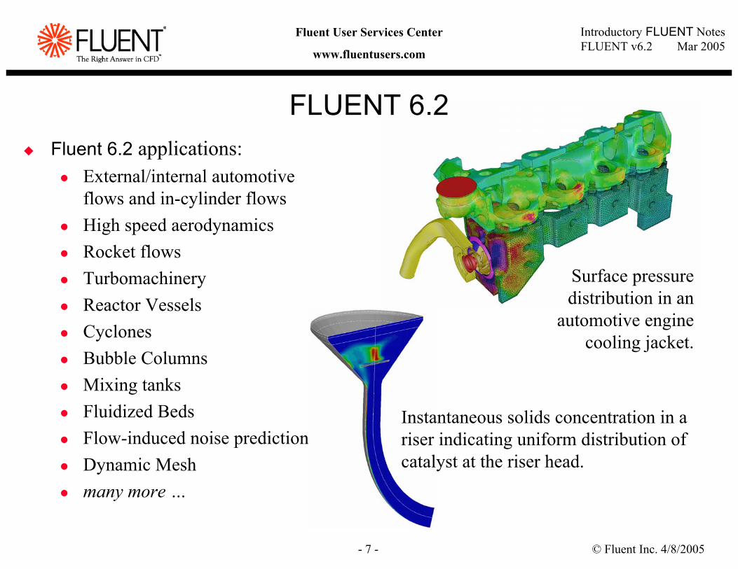
FLUENT 6.2Fluent 6.2 applications:

External/internal automotive flows and in-cylinder flowsHigh speed aerodynamicsRocket flowsTurbomachineryReactor VesselsCyclonesBubble ColumnsMixing tanksFluidized BedsFlow-induced noise predictionDynamic Meshmany more …

Surface pressure distribution in an

automotive engine cooling jacket.

Instantaneous solids concentration in a riser indicating uniform distribution of catalyst at the riser head.

© Fluent Inc. 4/8/2005- 8 -



www.fluentusers.com

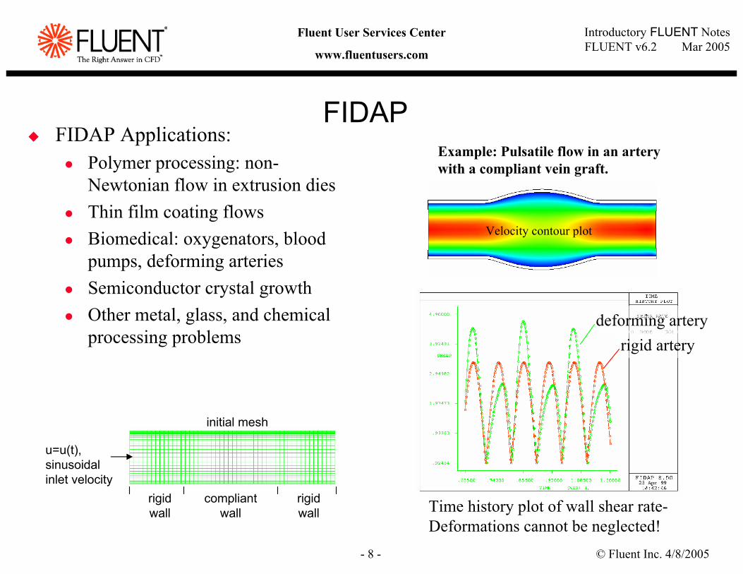
FIDAPFIDAP Applications:

Polymer processing: non-Newtonian flow in extrusion diesThin film coating flowsBiomedical: oxygenators, blood pumps, deforming arteriesSemiconductor crystal growthOther metal, glass, and chemical processing problems

Example: Pulsatile flow in an artery with a compliant vein graft.

u=u(t), sinusoidal inlet velocity

rigid wall

rigid wall

compliant wall

initial mesh

rigid arterydeforming artery

Time history plot of wall shear rate-Deformations cannot be neglected!

Velocity contour plot

© Fluent Inc. 4/8/2005- 9 -



www.fluentusers.com

POLYFLOW

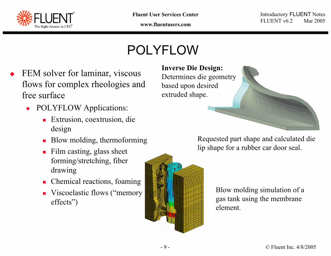
FEM solver for laminar, viscous flows for complex rheologies and free surface

POLYFLOW Applications:Extrusion, coextrusion, die designBlow molding, thermoformingFilm casting, glass sheet forming/stretching, fiber drawingChemical reactions, foamingViscoelastic flows (“memory effects”)

Inverse Die Design:Determines die geometry based upon desired extruded shape.

Requested part shape and calculated die lip shape for a rubber car door seal.

Blow molding simulation of a gas tank using the membrane element.

© Fluent Inc. 4/8/2005- 10 -



www.fluentusers.com

IcePak

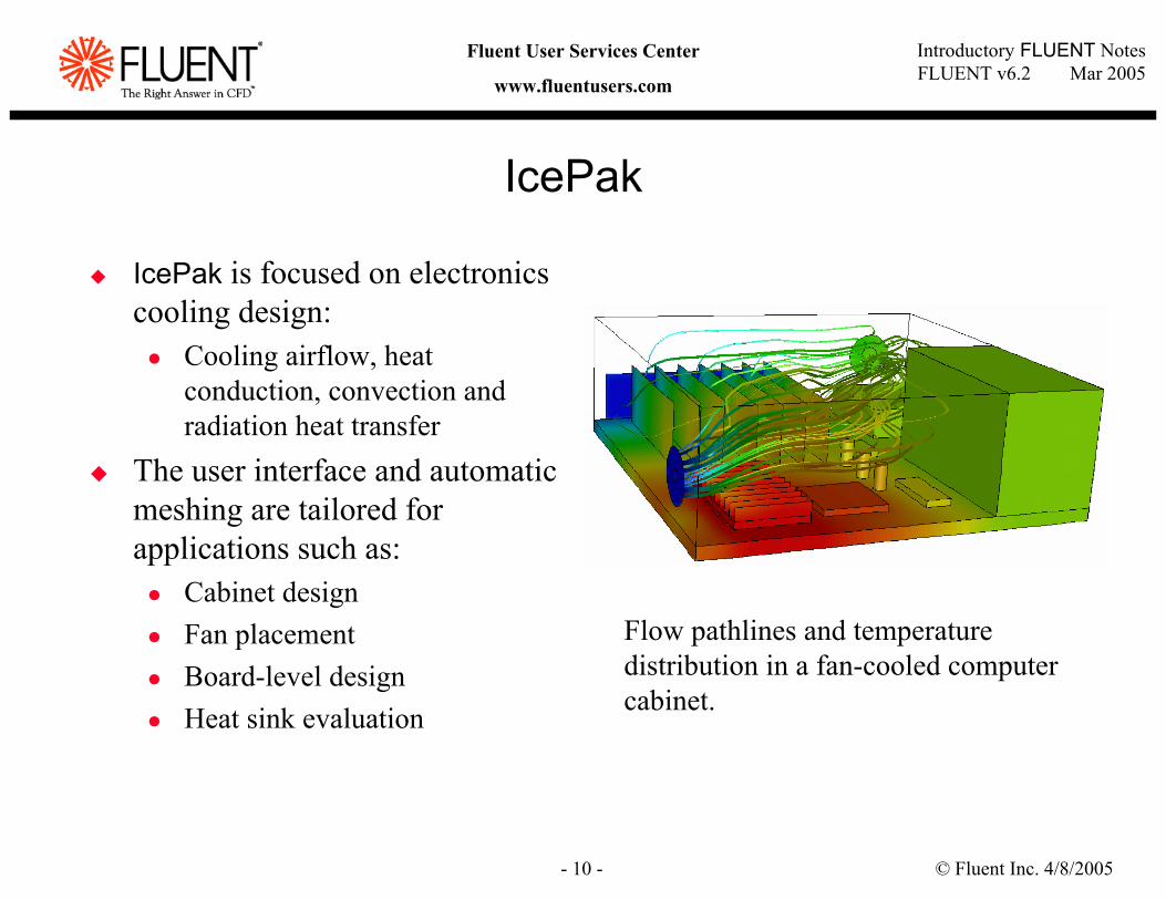
IcePak is focused on electronics cooling design:

Cooling airflow, heat conduction, convection and radiation heat transfer

The user interface and automatic meshing are tailored for applications such as:

Cabinet designFan placementBoard-level designHeat sink evaluation

Flow pathlines and temperature distribution in a fan-cooled computer cabinet.

© Fluent Inc. 4/8/2005- 11 -



www.fluentusers.com

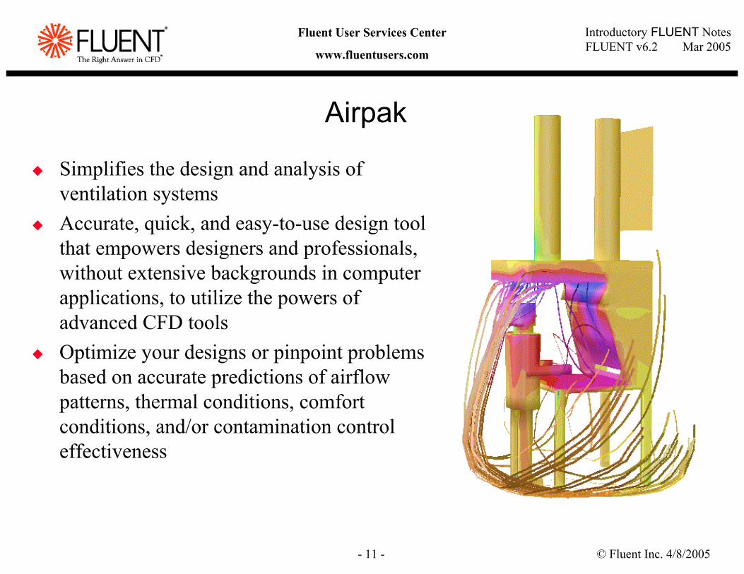
Simplifies the design and analysis of ventilation systemsAccurate, quick, and easy-to-use design tool that empowers designers and professionals, without extensive backgrounds in computer applications, to utilize the powers of advanced CFD toolsOptimize your designs or pinpoint problems based on accurate predictions of airflow patterns, thermal conditions, comfort conditions, and/or contamination control effectiveness

Airpak

© Fluent Inc. 4/8/2005- 12 -



www.fluentusers.com

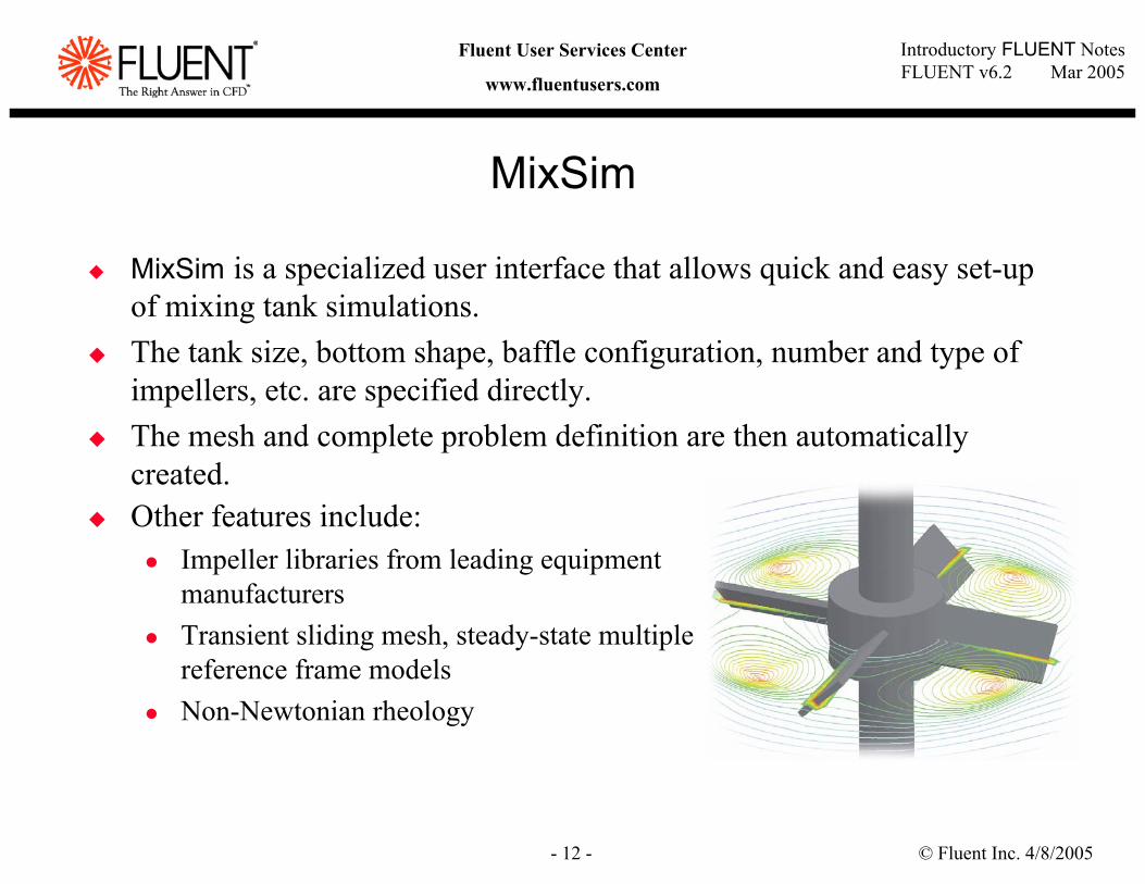
MixSim is a specialized user interface that allows quick and easy set-up of mixing tank simulations.The tank size, bottom shape, baffle configuration, number and type of impellers, etc. are specified directly.The mesh and complete problem definition are then automatically created.

MixSim

Other features include:Impeller libraries from leading equipment manufacturersTransient sliding mesh, steady-state multiple reference frame modelsNon-Newtonian rheology

© Fluent Inc. 4/8/2005- 13 -



www.fluentusers.com

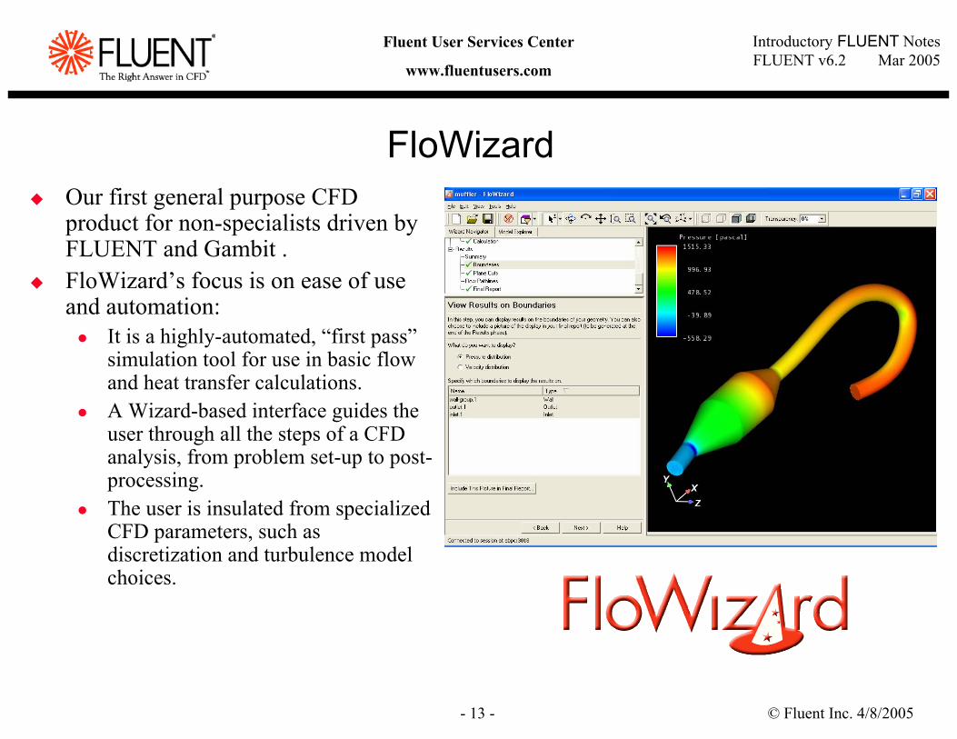
FloWizardOur first general purpose CFD product for non-specialists driven by FLUENT and Gambit .FloWizard’s focus is on ease of use and automation:

It is a highly-automated, “first pass”simulation tool for use in basic flow and heat transfer calculations.A Wizard-based interface guides the user through all the steps of a CFD analysis, from problem set-up to post-processing.The user is insulated from specialized CFD parameters, such as discretization and turbulence model choices.

© Fluent Inc. 4/8/2005- 14 -



www.fluentusers.com

A single, integrated pre-processor for CFD analysis.

Geometry creationMesh generationMesh quality examinationBoundary zone assignment

Pre-processor: Gambit

© Fluent Inc. 4/8/2005- 15 -



www.fluentusers.com

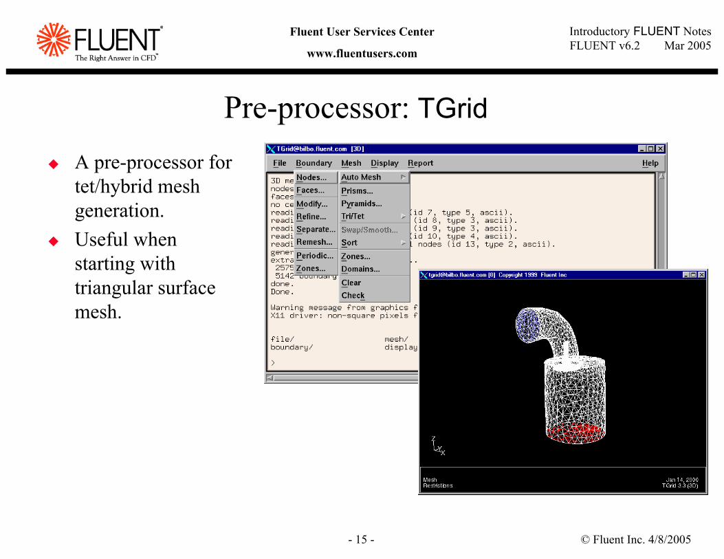
A pre-processor for tet/hybrid mesh generation.Useful when starting with triangular surface mesh.

Pre-processor: TGrid

© Fluent Inc. 4/8/2005- 16 -



www.fluentusers.com

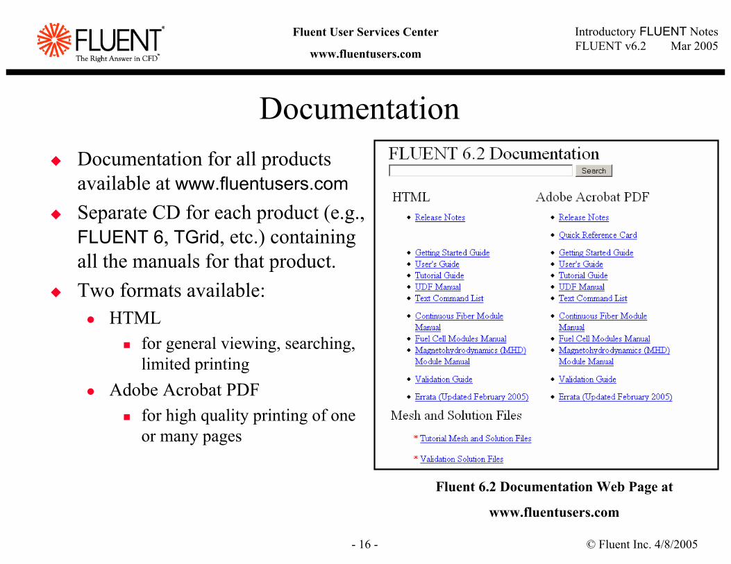
Documentation for all products available at www.fluentusers.comSeparate CD for each product (e.g., FLUENT 6, TGrid, etc.) containingall the manuals for that product.Two formats available:

HTMLfor general viewing, searching,limited printing

Adobe Acrobat PDFfor high quality printing of one or many pages

Documentation

Fluent 6.2 Documentation Web Page at

www.fluentusers.com

© Fluent Inc. 4/8/2005- 17 -



www.fluentusers.com

Introduction to CFD Analysis

© Fluent Inc. 4/8/2005- 18 -



www.fluentusers.com

What is CFD?

Computational Fluid Dynamics (CFD) is the science of predicting fluid flow, heat and mass transfer, chemical reactions, and related phenomena by solving numerically the set of governing mathematical equations.

Conservation of mass, momentum, energy, species, ...The results of CFD analyses are relevant in:

conceptual studies of new designsdetailed product developmenttroubleshootingredesign

CFD analysis complements testing and experimentation.Reduces the total effort required in the experiment design and data acquisition

© Fluent Inc. 4/8/2005- 19 -



www.fluentusers.com

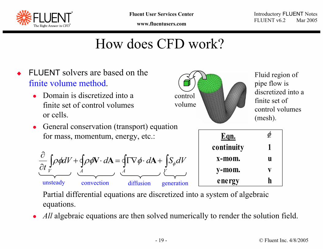
How does CFD work?

FLUENT solvers are based on thefinite volume method.

Domain is discretized into a finite set of control volumes or cells.General conservation (transport) equation for mass, momentum, energy, etc.:

Partial differential equations are discretized into a system of algebraic equations.All algebraic equations are then solved numerically to render the solution field.

∫∫∫∫ +⋅∇Γ=⋅+∂∂

VAAV

dVSdddVt φφρφρφ AAV

unsteady convection diffusion generation

Eqn.continuity 1

x-mom. uy-mom. venergy h

φ

Fluid region of pipe flow is discretized into a finite set of control volumes (mesh).

control volume

© Fluent Inc. 4/8/2005- 20 -



www.fluentusers.com

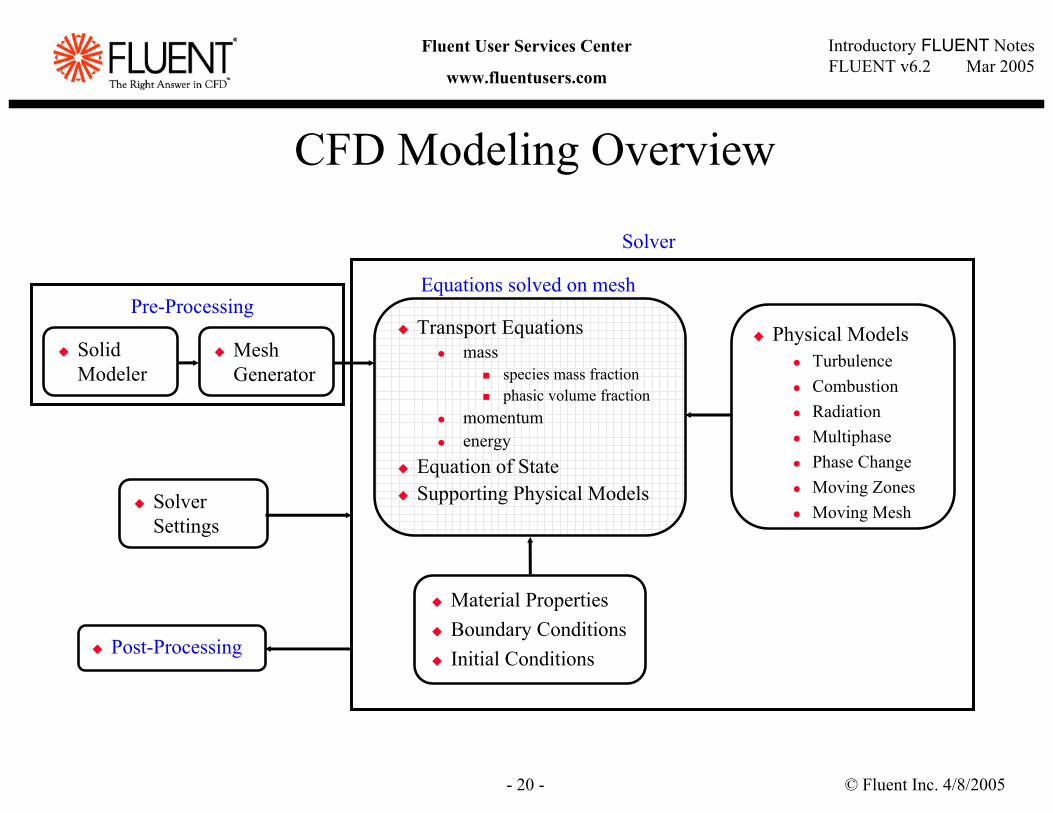
CFD Modeling Overview

Transport Equationsmass

species mass fractionphasic volume fraction

momentumenergy

Equation of StateSupporting Physical Models

Solver

Physical ModelsTurbulenceCombustionRadiationMultiphasePhase ChangeMoving ZonesMoving Mesh

Mesh Generator

Material PropertiesBoundary ConditionsInitial Conditions

Solver Settings

Pre-Processing

Solid Modeler

Post-Processing

Equations solved on mesh

© Fluent Inc. 4/8/2005- 21 -



www.fluentusers.com

CFD Analysis: Basic Steps

Problem Identification and Pre-Processing1. Define your modeling goals.2. Identify the domain you will model.3. Design and create the grid.Solver Execution4. Set up the numerical model.5. Compute and monitor the solution.Post-Processing6. Examine the results.7. Consider revisions to the model.

© Fluent Inc. 4/8/2005- 22 -



www.fluentusers.com

Define Your Modeling Goals

What results are you looking for, and how will they be used?What are your modeling options?

What physical models will need to be included in your analysis?What simplifying assumptions do you have to make?What simplifying assumptions can you make?Do you require a unique modeling capability?

User-defined functions (written in C) in FLUENT 6User-defined subroutines (written in FORTRAN) in FLUENT 4.5

What degree of accuracy is required?How quickly do you need the results?

Problem Identification and Pre-Processing1. Define your modeling goals.2. Identify the domain you will model.3. Design and create the grid.

© Fluent Inc. 4/8/2005- 23 -



www.fluentusers.com

Identify the Domain You Will Model

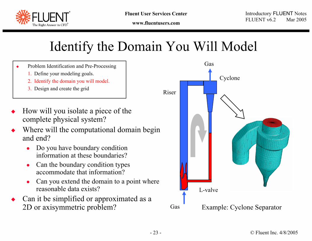
How will you isolate a piece of the complete physical system?Where will the computational domain begin and end?

Do you have boundary condition information at these boundaries?Can the boundary condition types accommodate that information?Can you extend the domain to a point where reasonable data exists?

Can it be simplified or approximated as a 2D or axisymmetric problem?

Problem Identification and Pre-Processing1. Define your modeling goals.2. Identify the domain you will model.3. Design and create the grid

Gas

Riser

Cyclone

L-valve

Gas Example: Cyclone Separator

© Fluent Inc. 4/8/2005- 24 -



www.fluentusers.com

Design and Create the GridCan you benefit from Mixsim, Icepak, or Airpak?Can you use a quad/hex grid or should you use a tri/tet grid or hybrid grid?

How complex is the geometry and flow?Will you need a non-conformal interface?

What degree of grid resolution is required in each region of the domain?

Is the resolution sufficient for the geometry?Can you predict regions with high gradients?Will you use adaption to add resolution?

Do you have sufficient computer memory?How many cells are required?How many models will be used?

triangle quadrilateral

tetrahedron

pyramid prism/wedge

hexahedron

Problem Identification and Pre-Processing1. Define your modeling goals.2. Identify the domain you will model.3. Design and create the grid.

© Fluent Inc. 4/8/2005- 25 -



www.fluentusers.com

Tri/Tet vs. Quad/Hex Meshes

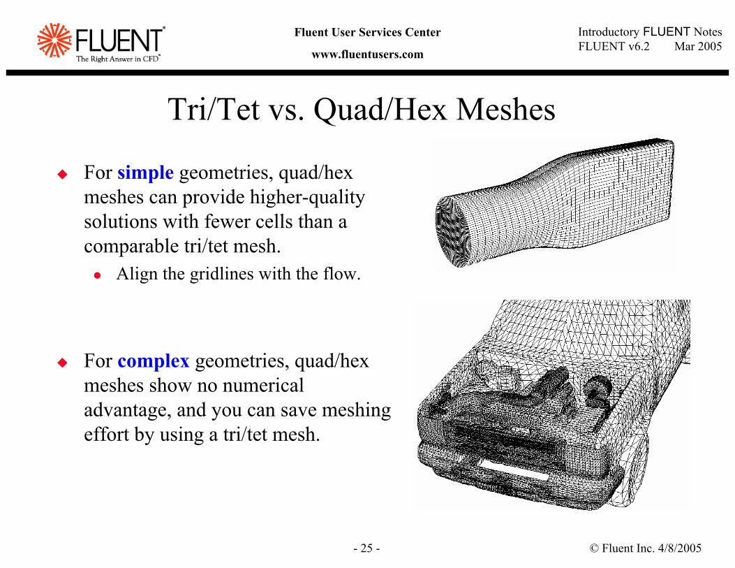
For simple geometries, quad/hex meshes can provide higher-quality solutions with fewer cells than a comparable tri/tet mesh.

Align the gridlines with the flow.

For complex geometries, quad/hex meshes show no numerical advantage, and you can save meshing effort by using a tri/tet mesh.

© Fluent Inc. 4/8/2005- 26 -



www.fluentusers.com

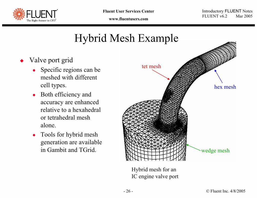
Hybrid Mesh Example

Valve port gridSpecific regions can be meshed with different cell types.Both efficiency and accuracy are enhanced relative to a hexahedral or tetrahedral mesh alone.Tools for hybrid mesh generation are available in Gambit and TGrid.

Hybrid mesh for an IC engine valve port

tet mesh

hex mesh

wedge mesh

© Fluent Inc. 4/8/2005- 27 -



www.fluentusers.com

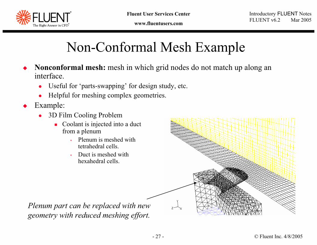
Non-Conformal Mesh ExampleNonconformal mesh: mesh in which grid nodes do not match up along an interface.

Useful for ‘parts-swapping’ for design study, etc.Helpful for meshing complex geometries.

Example:3D Film Cooling Problem

Coolant is injected into a ductfrom a plenum

Plenum is meshed withtetrahedral cells.Duct is meshed withhexahedral cells.

Plenum part can be replaced with new geometry with reduced meshing effort.

© Fluent Inc. 4/8/2005- 28 -



www.fluentusers.com

Set Up the Numerical Model

For a given problem, you will need to:Select appropriate physical models.

Turbulence, combustion, multiphase, etc.Define material properties.

Fluid SolidMixture

Prescribe operating conditions.Prescribe boundary conditions at all boundary zones.Provide an initial solution.Set up solver controls.Set up convergence monitors.

Solver Execution4. Set up the numerical model.5. Compute and monitor the solution.

Solving initially in 2D will provide valuable experience with the models and solver settings for your problem in a short amount of time.

© Fluent Inc. 4/8/2005- 29 -



www.fluentusers.com

Compute the SolutionThe discretized conservation equations are solved iteratively.

A number of iterations are usually required to reach a converged solution.

Convergence is reached when:Changes in solution variables from one iteration to the next are negligible.

Residuals provide a mechanism to help monitor this trend.

Overall property conservation is achieved.The accuracy of a converged solution is dependent upon:

Appropriateness and accuracy of physical models.Grid resolution and independenceProblem setup

Solver Execution4. Set up the numerical model.5. Compute and monitor the solution.

A converged and grid-independent solution on a well-posed problem will provide useful engineering results!

© Fluent Inc. 4/8/2005- 30 -



www.fluentusers.com

Examine the ResultsExamine the results to review solution and extract useful data.

Visualization Tools can be used to answer such questions as:

What is the overall flow pattern?Is there separation?Where do shocks, shear layers, etc. form?Are key flow features being resolved?

Numerical Reporting Tools can be used to calculate quantitative results:

Forces and MomentsAverage heat transfer coefficientsSurface and Volume integrated quantitiesFlux Balances

Post-Processing6. Examine the results.7. Consider revisions to the model.

Examine results to ensure property conservation and correct physical behavior. High residuals may be attributable to only a few cells of poor quality.

© Fluent Inc. 4/8/2005- 31 -



www.fluentusers.com

Consider Revisions to the ModelAre physical models appropriate?

Is flow turbulent?Is flow unsteady?Are there compressibility effects?Are there 3D effects?

Are boundary conditions correct?Is the computational domain large enough?Are boundary conditions appropriate?Are boundary values reasonable?

Is grid adequate?Can grid be adapted to improve results?Does solution change significantly with adaption, or is the solution grid independent?Does boundary resolution need to be improved?

Post-Processing6. Examine the results.7. Consider revisions to the model.

© Fluent Inc. 4/8/2005- 32 -



www.fluentusers.com

FLUENT DEMO

Startup Gambit (Pre-processing)load databasedefine boundary zonesexport mesh

Startup Fluent (Solver Execution)GUIProblem SetupSolve

Post-ProcessingOnline Documentation

© Fluent Inc. 4/8/2005- 33 -



www.fluentusers.com

Navigating the PC at FluentLogin as fluent; password: fluentDirectories

Session will start in D:\users\fluentChange directory to and save work in D:\users\fluent\fluent

Or in the following areas:Fluent tutorial mesh files are in D:\users\fluent\fluent\tutGambit tutorial mesh files are in D:\users\fluent\fluent\gambit\tut

To start Fluent 6 / Gambit2:From startup menu: Programs → fluent inc → fluentFrom command prompt: fluent 2d or fluent 3d

Your support engineer will save your work at the end of the week.!Note: It is recommended that you restart fluent for each tutorial to avoid mixing solver settings from different tutorials.

© Fluent Inc. 4/8/2005- 34 -



www.fluentusers.com

Solver Basics

© Fluent Inc. 4/8/2005- 35 -



www.fluentusers.com

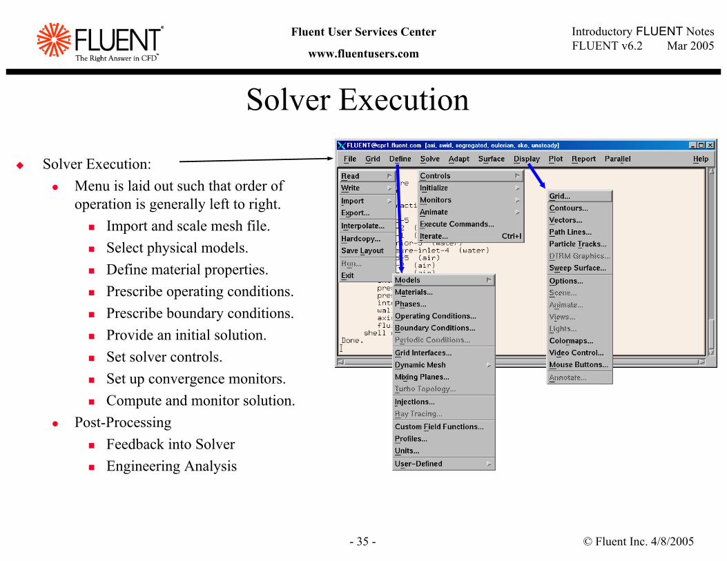
Solver Execution

Solver Execution:Menu is laid out such that order of operation is generally left to right.

Import and scale mesh file.Select physical models.Define material properties.Prescribe operating conditions.Prescribe boundary conditions.Provide an initial solution.Set solver controls.Set up convergence monitors.Compute and monitor solution.

Post-ProcessingFeedback into SolverEngineering Analysis

© Fluent Inc. 4/8/2005- 36 -



www.fluentusers.com

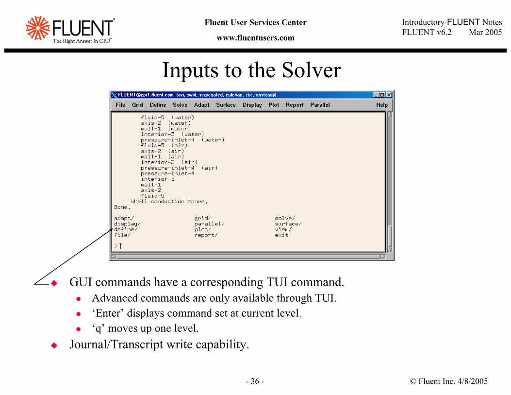
Inputs to the Solver

GUI commands have a corresponding TUI command.Advanced commands are only available through TUI.‘Enter’ displays command set at current level.‘q’ moves up one level.

Journal/Transcript write capability.

© Fluent Inc. 4/8/2005- 37 -



www.fluentusers.com

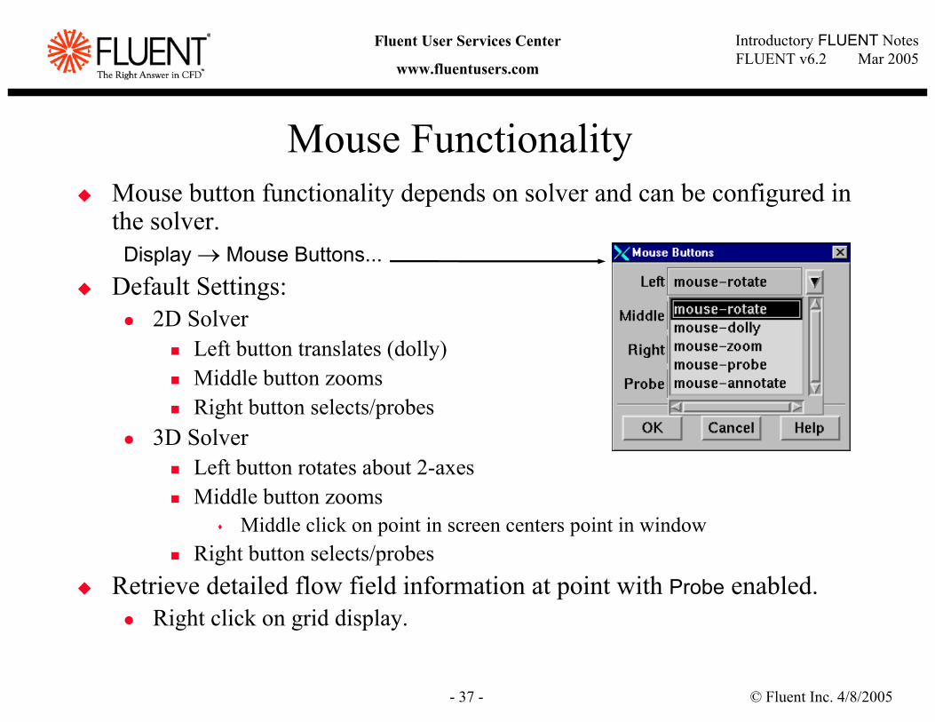
Mouse FunctionalityMouse button functionality depends on solver and can be configured in the solver.

Display → Mouse Buttons...Default Settings:

2D SolverLeft button translates (dolly)Middle button zoomsRight button selects/probes

3D SolverLeft button rotates about 2-axesMiddle button zooms

Middle click on point in screen centers point in windowRight button selects/probes

Retrieve detailed flow field information at point with Probe enabled.Right click on grid display.

© Fluent Inc. 4/8/2005- 38 -



www.fluentusers.com

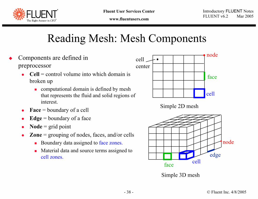
Reading Mesh: Mesh ComponentsComponents are defined in preprocessor

Cell = control volume into which domain is broken up

computational domain is defined by mesh that represents the fluid and solid regions of interest.

Face = boundary of a cellEdge = boundary of a faceNode = grid pointZone = grouping of nodes, faces, and/or cells

Boundary data assigned to face zones.Material data and source terms assigned to cell zones.

face cell

node

edge

Simple 2D mesh

Simple 3D mesh

node

face

cell

cell center

© Fluent Inc. 4/8/2005- 39 -



www.fluentusers.com

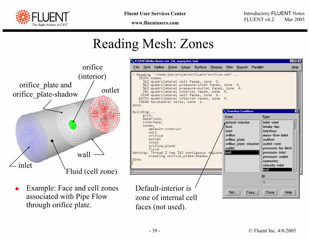
Reading Mesh: Zones

Example: Face and cell zones associated with Pipe Flow through orifice plate.

inlet

outlet

wall

orifice(interior)

orifice_plate and orifice_plate-shadow

Fluid (cell zone)

Default-interior is zone of internal cell faces (not used).

© Fluent Inc. 4/8/2005- 40 -



www.fluentusers.com

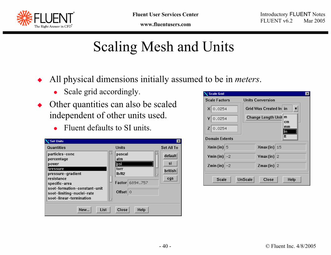
Scaling Mesh and Units

All physical dimensions initially assumed to be in meters.Scale grid accordingly.

Other quantities can also be scaled independent of other units used.

Fluent defaults to SI units.

© Fluent Inc. 4/8/2005- 41 -



www.fluentusers.com

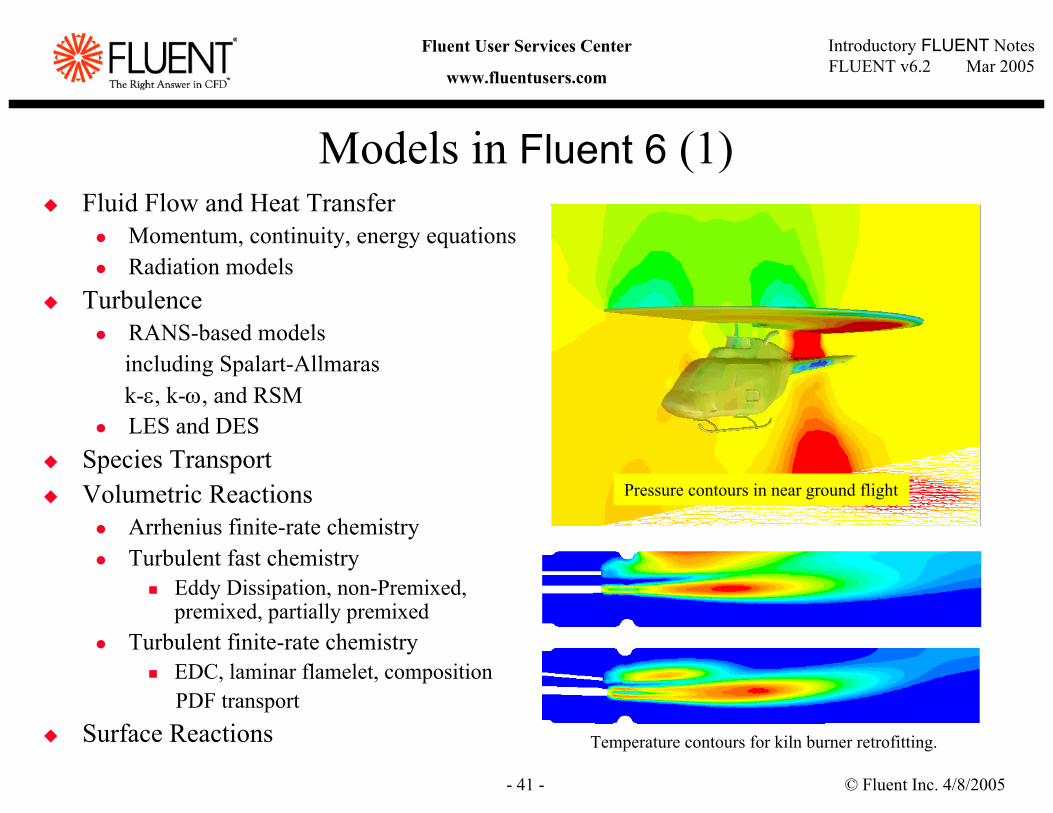
Fluid Flow and Heat TransferMomentum, continuity, energy equationsRadiation models

TurbulenceRANS-based modelsincluding Spalart-Allmarask-ε, k-ω, and RSMLES and DES

Species TransportVolumetric Reactions

Arrhenius finite-rate chemistryTurbulent fast chemistry

Eddy Dissipation, non-Premixed, premixed, partially premixed

Turbulent finite-rate chemistryEDC, laminar flamelet, composition PDF transport

Surface Reactions

Models in Fluent 6 (1)

Pressure contours in near ground flight

Temperature contours for kiln burner retrofitting.

© Fluent Inc. 4/8/2005- 42 -



www.fluentusers.com

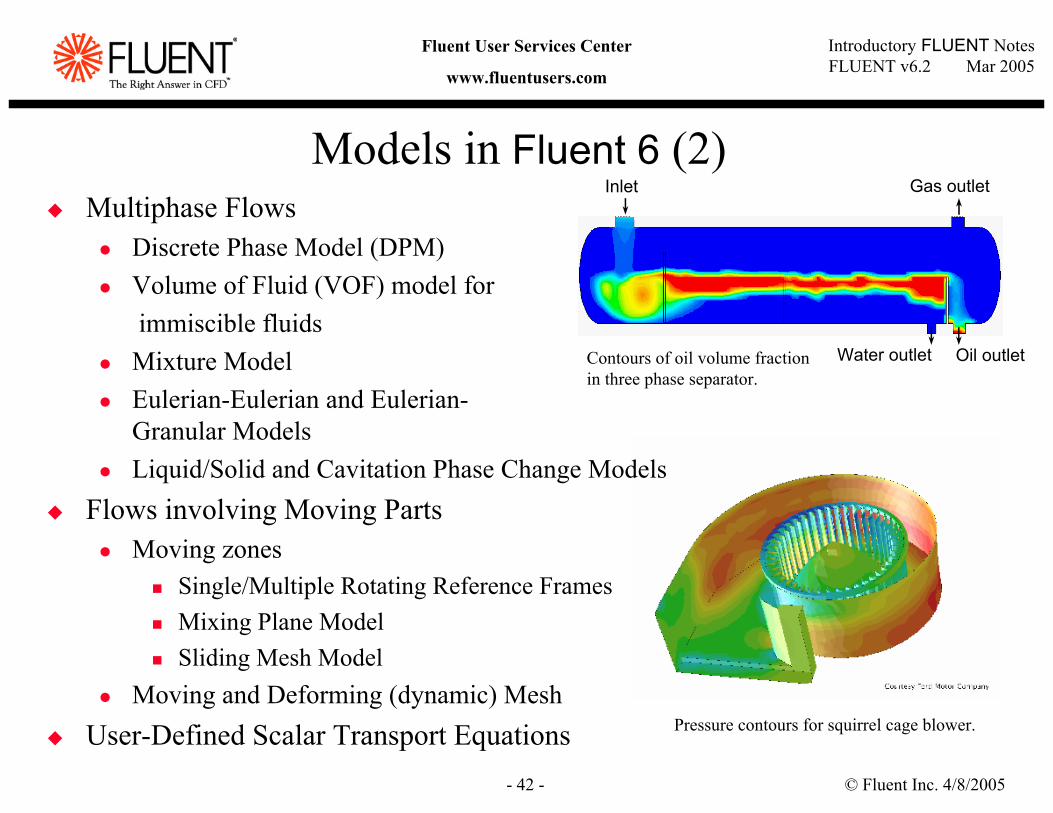
Multiphase FlowsDiscrete Phase Model (DPM)Volume of Fluid (VOF) model for immiscible fluids

Mixture ModelEulerian-Eulerian and Eulerian-Granular ModelsLiquid/Solid and Cavitation Phase Change Models

Flows involving Moving PartsMoving zones

Single/Multiple Rotating Reference FramesMixing Plane ModelSliding Mesh Model

Moving and Deforming (dynamic) MeshUser-Defined Scalar Transport Equations

Models in Fluent 6 (2)Gas outlet

Oil outlet

Inlet

Water outletContours of oil volume fraction in three phase separator.

Pressure contours for squirrel cage blower.

© Fluent Inc. 4/8/2005- 43 -



www.fluentusers.com

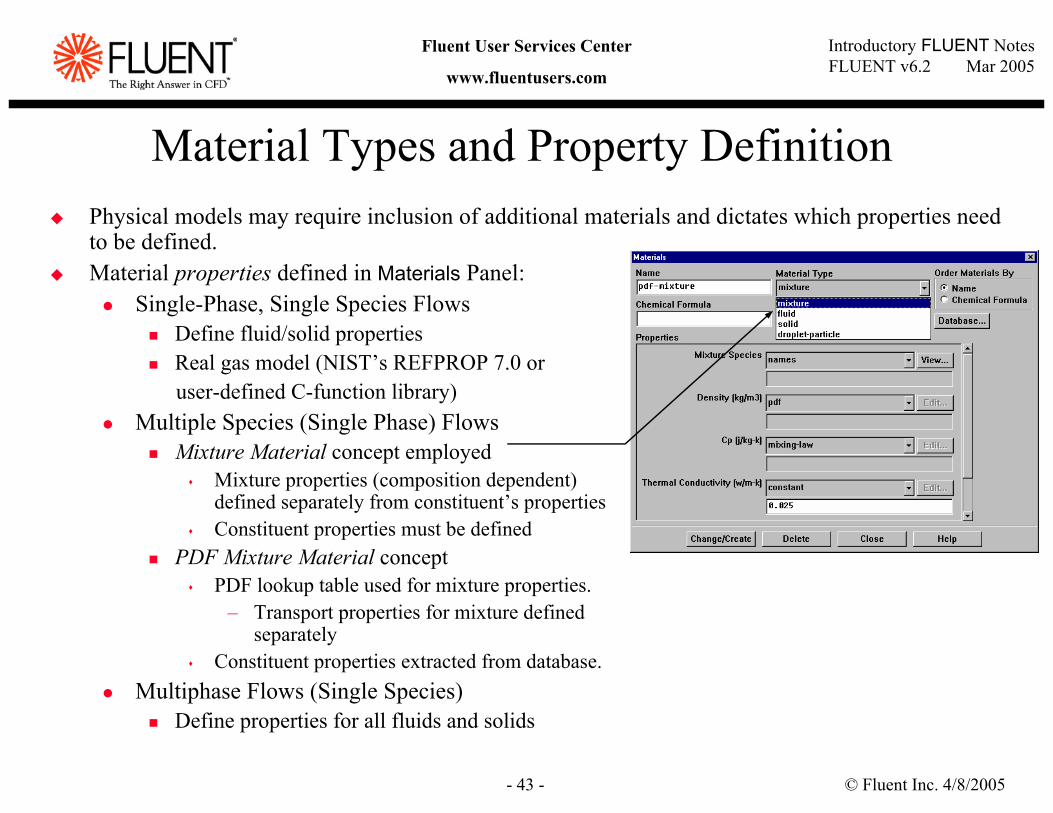
Material Types and Property DefinitionPhysical models may require inclusion of additional materials and dictates which properties need to be defined.Material properties defined in Materials Panel:

Single-Phase, Single Species FlowsDefine fluid/solid propertiesReal gas model (NIST’s REFPROP 7.0 or user-defined C-function library)

Multiple Species (Single Phase) FlowsMixture Material concept employed

Mixture properties (composition dependent) defined separately from constituent’s propertiesConstituent properties must be defined

PDF Mixture Material conceptPDF lookup table used for mixture properties.

– Transport properties for mixture defined separately

Constituent properties extracted from database.Multiphase Flows (Single Species)

Define properties for all fluids and solids

© Fluent Inc. 4/8/2005- 44 -



www.fluentusers.com

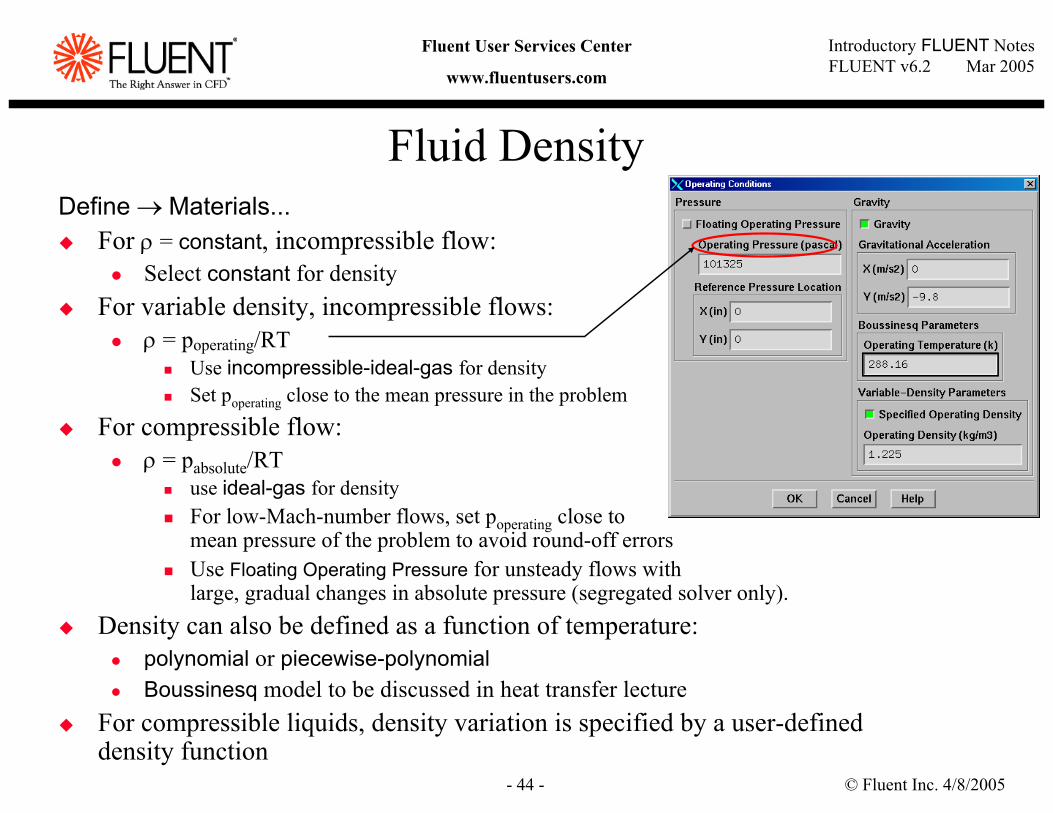
Fluid DensityDefine → Materials...

For ρ = constant, incompressible flow:Select constant for density

For variable density, incompressible flows: ρ = poperating/RT

Use incompressible-ideal-gas for densitySet poperating close to the mean pressure in the problem

For compressible flow:ρ = pabsolute/RT

use ideal-gas for densityFor low-Mach-number flows, set poperating close to mean pressure of the problem to avoid round-off errorsUse Floating Operating Pressure for unsteady flows with large, gradual changes in absolute pressure (segregated solver only).

Density can also be defined as a function of temperature:polynomial or piecewise-polynomialBoussinesq model to be discussed in heat transfer lecture

For compressible liquids, density variation is specified by a user-defined density function

© Fluent Inc. 4/8/2005- 45 -



www.fluentusers.com

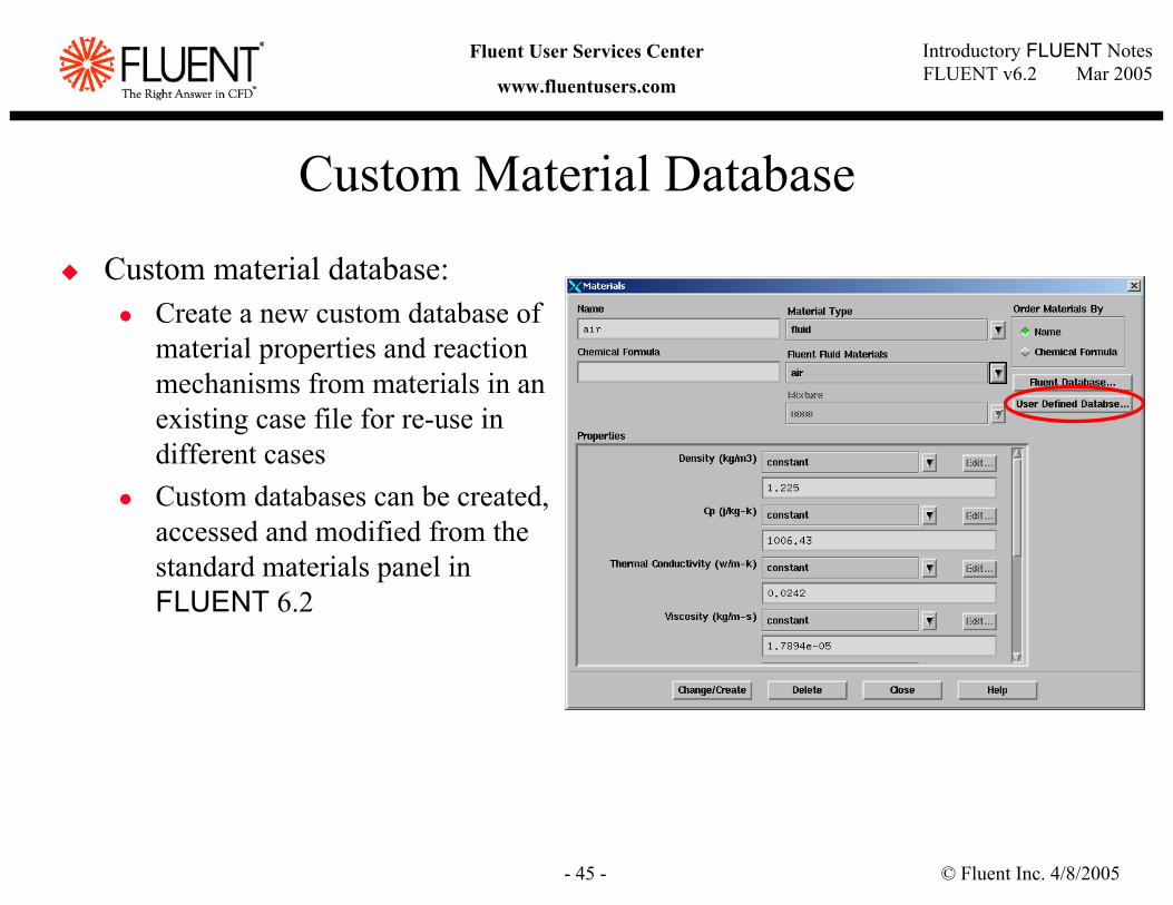
Custom Material Database

Custom material database: Create a new custom database of material properties and reaction mechanisms from materials in an existing case file for re-use in different cases Custom databases can be created, accessed and modified from the standard materials panel in FLUENT 6.2

© Fluent Inc. 4/8/2005- 46 -



www.fluentusers.com

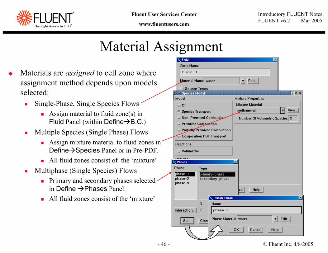
Material Assignment

Materials are assigned to cell zone where assignment method depends upon models selected:

Single-Phase, Single Species FlowsAssign material to fluid zone(s) in Fluid Panel (within Define B.C.)

Multiple Species (Single Phase) FlowsAssign mixture material to fluid zones in Define Species Panel or in Pre-PDF.All fluid zones consist of the ‘mixture’

Multiphase (Single Species) FlowsPrimary and secondary phases selectedin Define Phases Panel.All fluid zones consist of the ‘mixture’

© Fluent Inc. 4/8/2005- 47 -



www.fluentusers.com

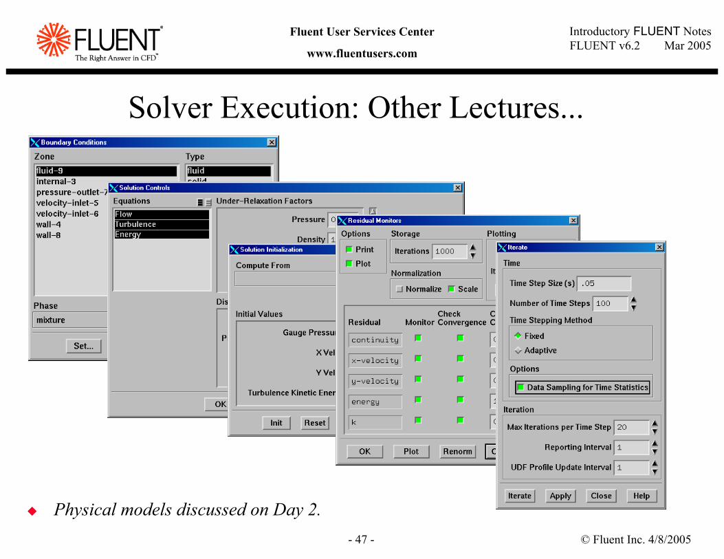
Solver Execution: Other Lectures...

Physical models discussed on Day 2.

© Fluent Inc. 4/8/2005- 48 -



www.fluentusers.com

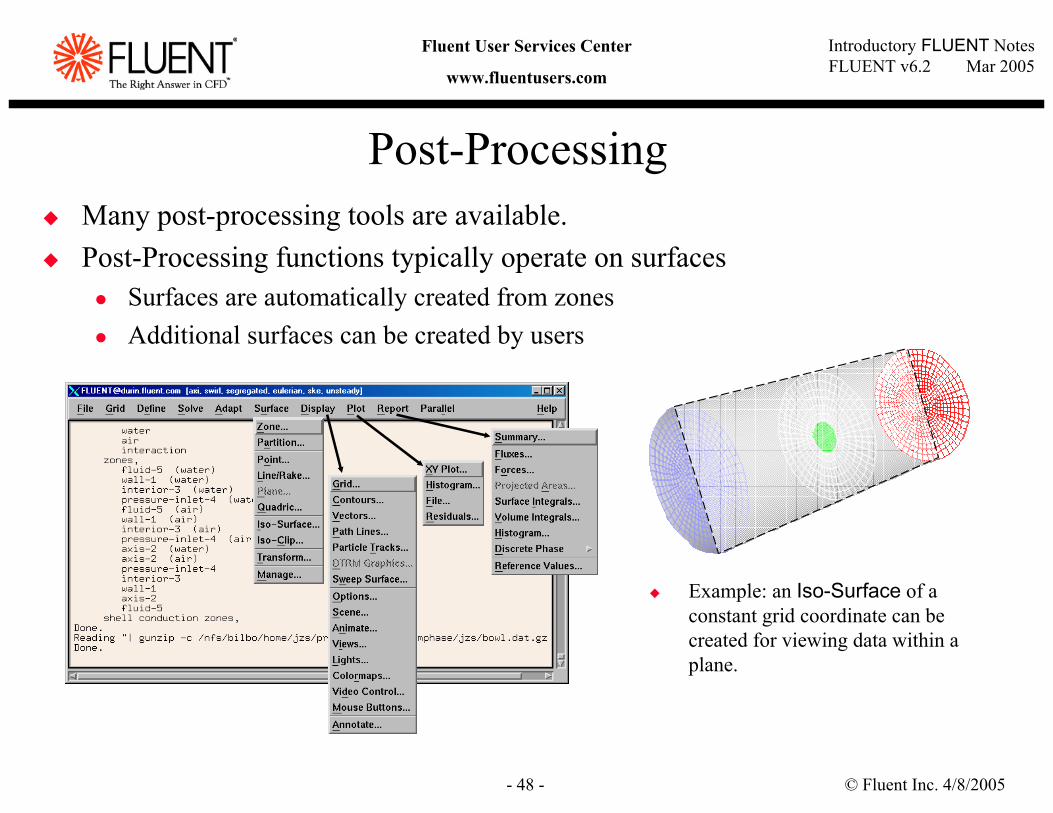
Post-ProcessingMany post-processing tools are available.Post-Processing functions typically operate on surfaces

Surfaces are automatically created from zonesAdditional surfaces can be created by users

Example: an Iso-Surface of a constant grid coordinate can be created for viewing data within a plane.

© Fluent Inc. 4/8/2005- 49 -



www.fluentusers.com

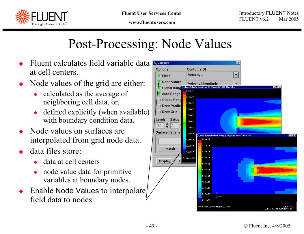
Post-Processing: Node ValuesFluent calculates field variable data at cell centers.Node values of the grid are either:

calculated as the average of neighboring cell data, or,defined explicitly (when available) with boundary condition data.

Node values on surfaces are interpolated from grid node data.data files store:

data at cell centersnode value data for primitive variables at boundary nodes.

Enable Node Values to interpolate field data to nodes.

© Fluent Inc. 4/8/2005- 50 -



www.fluentusers.com

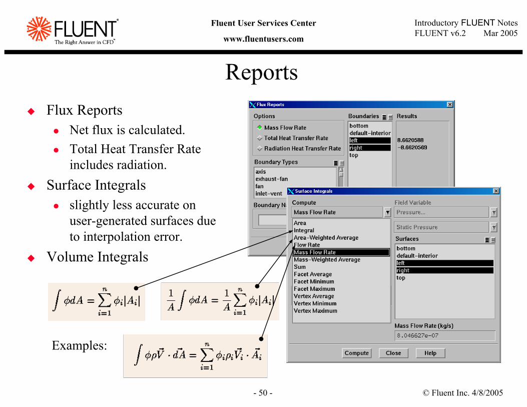
ReportsFlux Reports

Net flux is calculated.Total Heat Transfer Rate includes radiation.

Surface Integralsslightly less accurate on user-generated surfaces due to interpolation error.

Volume Integrals

Examples:

© Fluent Inc. 4/8/2005- 51 -



www.fluentusers.com

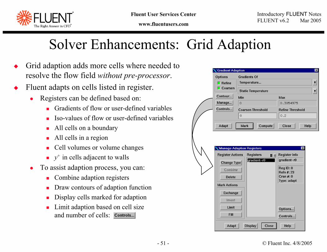
Solver Enhancements: Grid AdaptionGrid adaption adds more cells where needed to resolve the flow field without pre-processor.Fluent adapts on cells listed in register.

Registers can be defined based on:Gradients of flow or user-defined variablesIso-values of flow or user-defined variablesAll cells on a boundaryAll cells in a regionCell volumes or volume changesy+ in cells adjacent to walls

To assist adaption process, you can:Combine adaption registersDraw contours of adaption functionDisplay cells marked for adaptionLimit adaption based on cell sizeand number of cells:

© Fluent Inc. 4/8/2005- 52 -



www.fluentusers.com

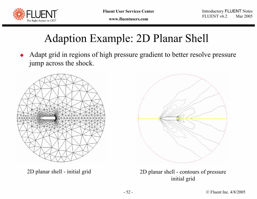
Adaption Example: 2D Planar Shell

2D planar shell - initial grid

Adapt grid in regions of high pressure gradient to better resolve pressure jump across the shock.

2D planar shell - contours of pressure initial grid

© Fluent Inc. 4/8/2005- 53 -



www.fluentusers.com

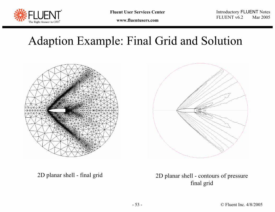
Adaption Example: Final Grid and Solution

2D planar shell - contours of pressure final grid

2D planar shell - final grid

© Fluent Inc. 4/8/2005- 54 -



www.fluentusers.com

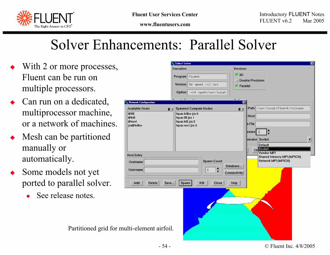
Solver Enhancements: Parallel SolverWith 2 or more processes, Fluent can be run on multiple processors.Can run on a dedicated, multiprocessor machine, or a network of machines.Mesh can be partitioned manually or automatically.Some models not yet ported to parallel solver.

See release notes.

Partitioned grid for multi-element airfoil.

© Fluent Inc. 4/8/2005- 55 -



www.fluentusers.com

Boundary Conditions

© Fluent Inc. 4/8/2005- 56 -



www.fluentusers.com

Defining Boundary ConditionsTo define a problem that results in a unique solution, you must specify information on the dependent (flow) variables at the domain boundaries

Specifying fluxes of mass, momentum, energy, etc. into domain.Defining boundary conditions involves:

identifying the location of the boundaries (e.g., inlets, walls, symmetry)supplying information at the boundaries

The data required at a boundary depends upon the boundary condition type and the physical models employed.You must be aware of the information that is required of the boundary condition and locate the boundaries where the information on the flow variables are known or can be reasonably approximated

Poorly defined boundary conditions can have a significant impact on your solution

© Fluent Inc. 4/8/2005- 57 -



www.fluentusers.com

Fuel

Air

Combustor Wall

Manifold box

1

1

23

Nozzle

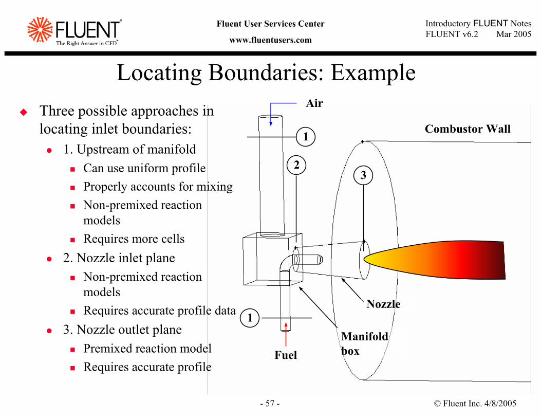
Locating Boundaries: ExampleThree possible approaches in locating inlet boundaries:

1. Upstream of manifoldCan use uniform profileProperly accounts for mixingNon-premixed reaction modelsRequires more cells

2. Nozzle inlet planeNon-premixed reaction modelsRequires accurate profile data

3. Nozzle outlet planePremixed reaction modelRequires accurate profile

© Fluent Inc. 4/8/2005- 58 -



www.fluentusers.com

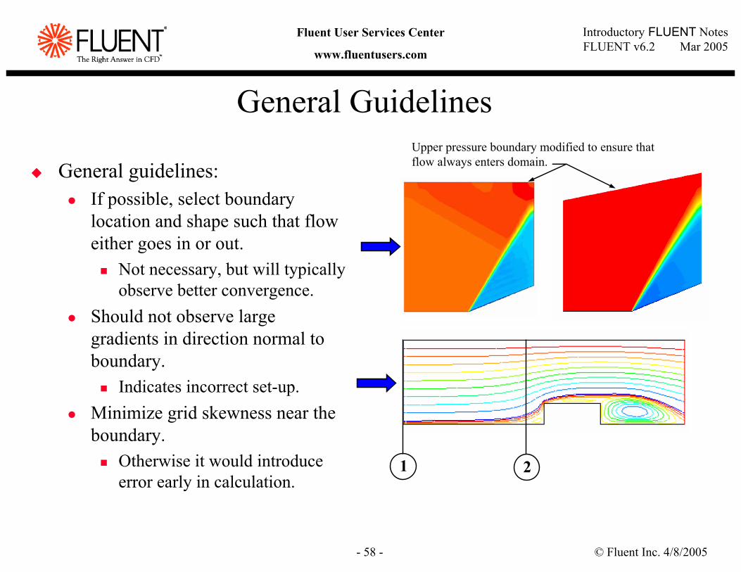
General Guidelines

General guidelines:If possible, select boundary location and shape such that flow either goes in or out.

Not necessary, but will typically observe better convergence.

Should not observe large gradients in direction normal to boundary.

Indicates incorrect set-up.Minimize grid skewness near the boundary.

Otherwise it would introduce error early in calculation.

21

Upper pressure boundary modified to ensure that flow always enters domain.

© Fluent Inc. 4/8/2005- 59 -



www.fluentusers.com

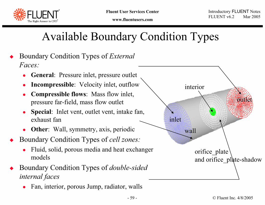
Available Boundary Condition TypesBoundary Condition Types of External Faces:

General: Pressure inlet, pressure outletIncompressible: Velocity inlet, outflowCompressible flows: Mass flow inlet, pressure far-field, mass flow outletSpecial: Inlet vent, outlet vent, intake fan, exhaust fanOther: Wall, symmetry, axis, periodic

Boundary Condition Types of cell zones:Fluid, solid, porous media and heat exchanger models

Boundary Condition Types of double-sided internal faces

Fan, interior, porous Jump, radiator, walls

inlet

outlet

wall

interior

orifice_plate and orifice_plate-shadow

© Fluent Inc. 4/8/2005- 60 -



www.fluentusers.com

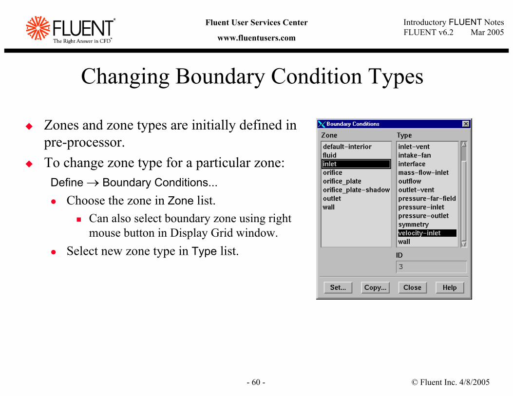
Changing Boundary Condition Types

Zones and zone types are initially defined in pre-processor.To change zone type for a particular zone:

Define → Boundary Conditions...Choose the zone in Zone list.

Can also select boundary zone using right mouse button in Display Grid window.

Select new zone type in Type list.

© Fluent Inc. 4/8/2005- 61 -



www.fluentusers.com

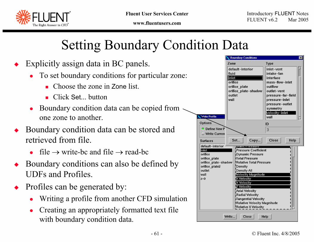
Setting Boundary Condition DataExplicitly assign data in BC panels.

To set boundary conditions for particular zone:Choose the zone in Zone list.Click Set... button

Boundary condition data can be copied from one zone to another.

Boundary condition data can be stored and retrieved from file.

file → write-bc and file → read-bcBoundary conditions can also be defined by UDFs and Profiles.Profiles can be generated by:

Writing a profile from another CFD simulationCreating an appropriately formatted text file with boundary condition data.

© Fluent Inc. 4/8/2005- 62 -



www.fluentusers.com

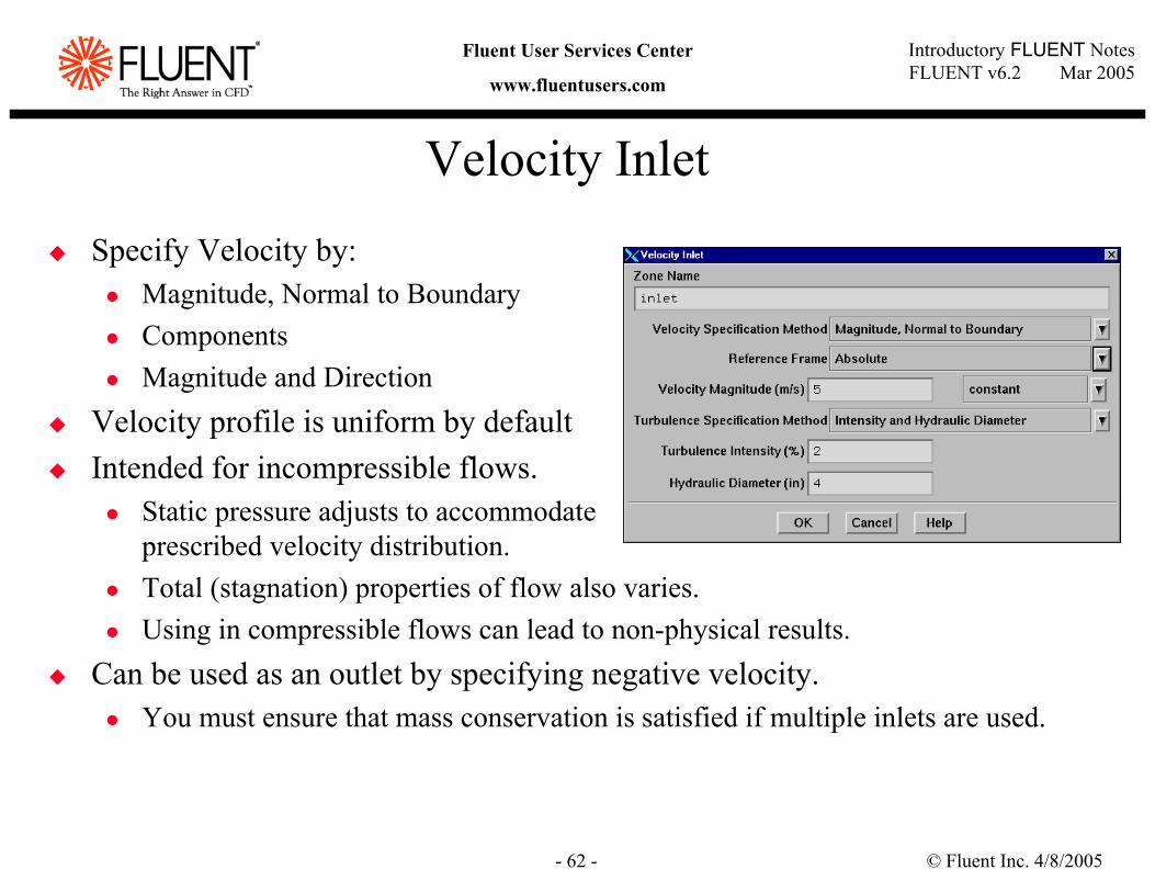
Velocity Inlet

Specify Velocity by:Magnitude, Normal to BoundaryComponentsMagnitude and Direction

Velocity profile is uniform by defaultIntended for incompressible flows.

Static pressure adjusts to accommodate prescribed velocity distribution.Total (stagnation) properties of flow also varies.Using in compressible flows can lead to non-physical results.

Can be used as an outlet by specifying negative velocity.You must ensure that mass conservation is satisfied if multiple inlets are used.

© Fluent Inc. 4/8/2005- 63 -



www.fluentusers.com

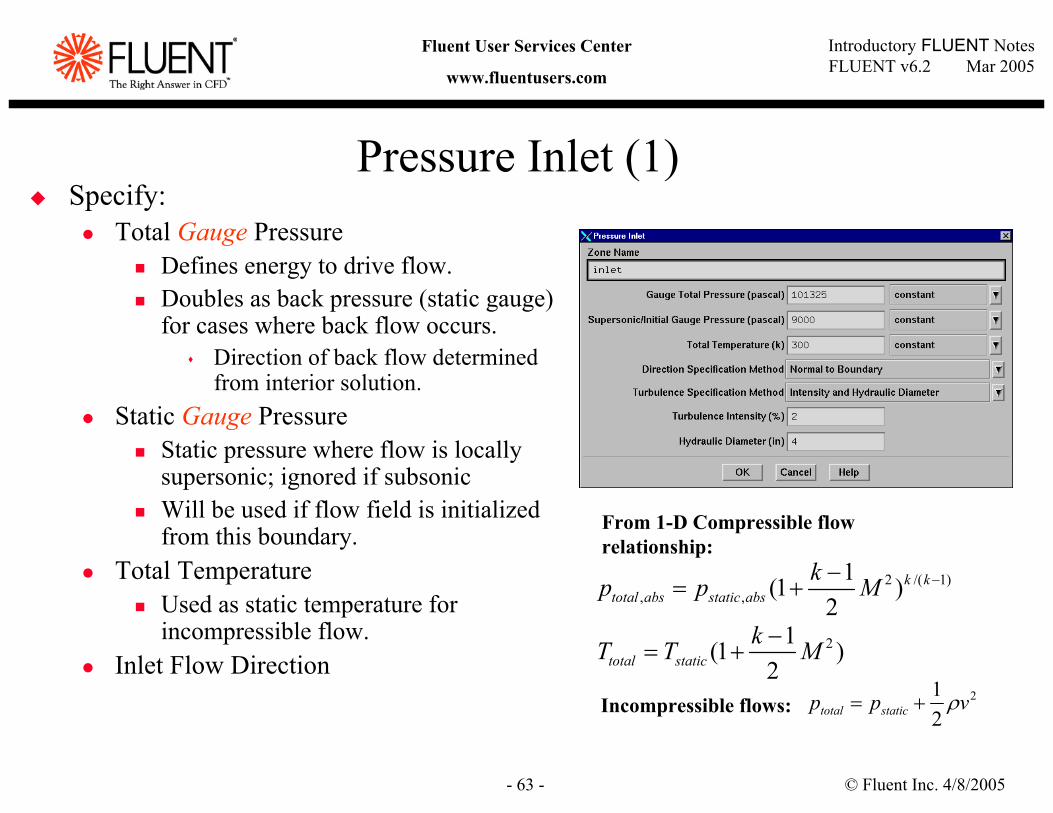
Pressure Inlet (1)Specify:

Total Gauge PressureDefines energy to drive flow.Doubles as back pressure (static gauge) for cases where back flow occurs.

Direction of back flow determined from interior solution.

Static Gauge PressureStatic pressure where flow is locally supersonic; ignored if subsonicWill be used if flow field is initialized from this boundary.

Total TemperatureUsed as static temperature for incompressible flow.

Inlet Flow Direction21(1 )

2total statickT T M−

= +

2 /( 1), ,

1(1 )2

k ktotal abs static abs

kp p M −−= +

2

21 vpp statictotal ρ+=Incompressible flows:

From 1-D Compressible flow relationship:

© Fluent Inc. 4/8/2005- 64 -



www.fluentusers.com

Pressure Inlet (2)

Note: Gauge pressure inputs are required.

Operating pressure level sometimes may affect solution accuracy (when pressure fluctuations are relatively small).Operating pressure input is set under: Define → Operating Conditions

Suitable for compressible and incompressible flows.Pressure inlet boundary is treated as loss-free transition from stagnation to inlet conditions.Fluent calculates static pressure and velocity at inletMass flux through boundary varies depending on interior solution and specified flow direction.

Can be used as a “free” boundary in an external or unconfined flow.

operatinggaugeabsolute ppp +=

© Fluent Inc. 4/8/2005- 65 -



www.fluentusers.com

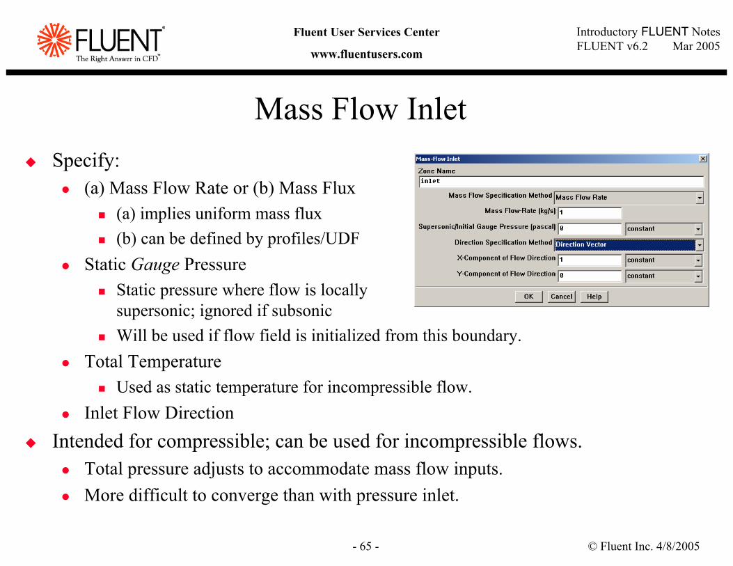
Mass Flow InletSpecify:

(a) Mass Flow Rate or (b) Mass Flux(a) implies uniform mass flux(b) can be defined by profiles/UDF

Static Gauge PressureStatic pressure where flow is locallysupersonic; ignored if subsonicWill be used if flow field is initialized from this boundary.

Total TemperatureUsed as static temperature for incompressible flow.

Inlet Flow DirectionIntended for compressible; can be used for incompressible flows.

Total pressure adjusts to accommodate mass flow inputs.More difficult to converge than with pressure inlet.

© Fluent Inc. 4/8/2005- 66 -



www.fluentusers.com

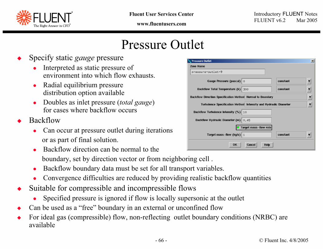
Pressure OutletSpecify static gauge pressure

Interpreted as static pressure of environment into which flow exhausts.Radial equilibrium pressuredistribution option availableDoubles as inlet pressure (total gauge)for cases where backflow occurs

BackflowCan occur at pressure outlet during iterations or as part of final solution.Backflow direction can be normal to the boundary, set by direction vector or from neighboring cell .Backflow boundary data must be set for all transport variables.Convergence difficulties are reduced by providing realistic backflow quantities

Suitable for compressible and incompressible flowsSpecified pressure is ignored if flow is locally supersonic at the outlet

Can be used as a “free” boundary in an external or unconfined flowFor ideal gas (compressible) flow, non-reflecting outlet boundary conditions (NRBC) are available

© Fluent Inc. 4/8/2005- 67 -



www.fluentusers.com

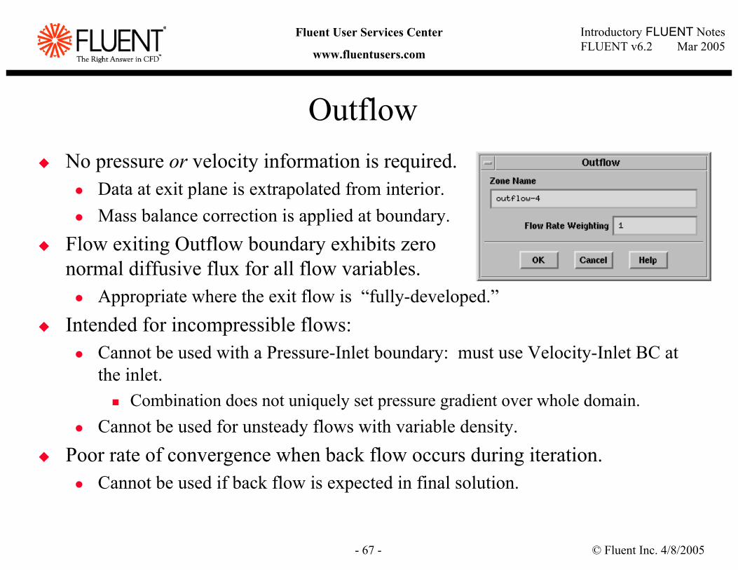
OutflowNo pressure or velocity information is required.

Data at exit plane is extrapolated from interior.Mass balance correction is applied at boundary.

Flow exiting Outflow boundary exhibits zero normal diffusive flux for all flow variables.

Appropriate where the exit flow is “fully-developed.”Intended for incompressible flows:

Cannot be used with a Pressure-Inlet boundary: must use Velocity-Inlet BC at the inlet.

Combination does not uniquely set pressure gradient over whole domain. Cannot be used for unsteady flows with variable density.

Poor rate of convergence when back flow occurs during iteration.Cannot be used if back flow is expected in final solution.

© Fluent Inc. 4/8/2005- 68 -



www.fluentusers.com

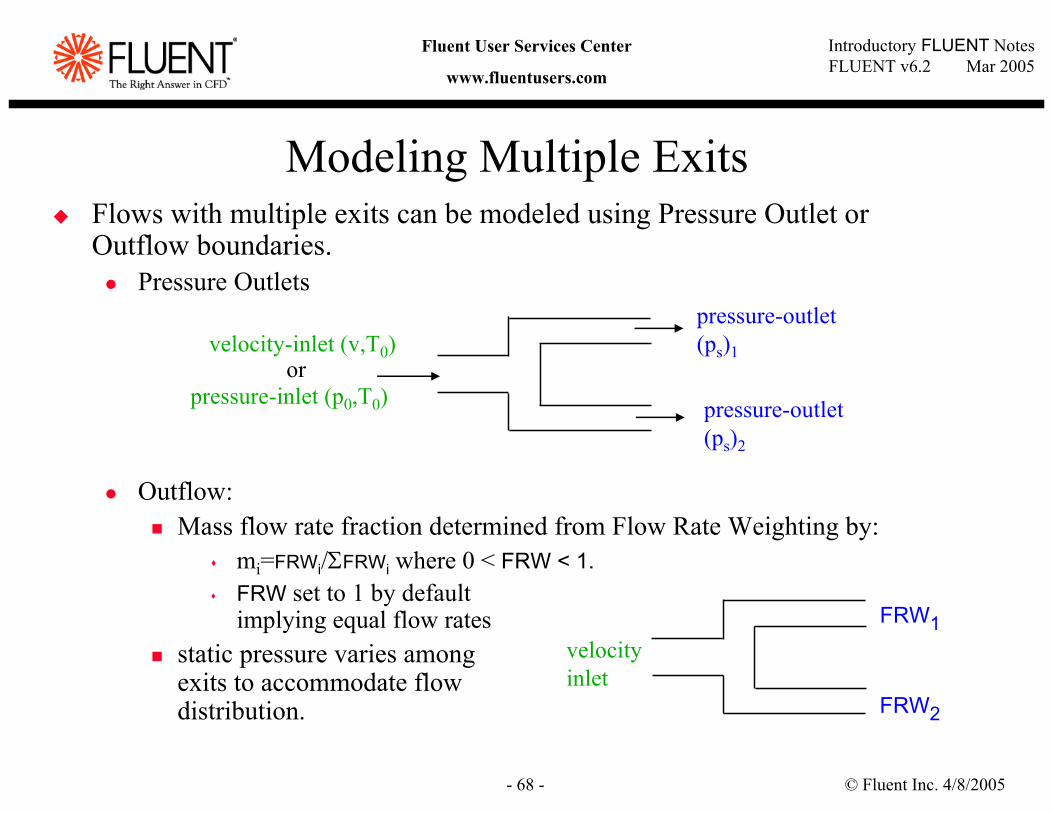
Modeling Multiple ExitsFlows with multiple exits can be modeled using Pressure Outlet or Outflow boundaries.

Pressure Outlets

Outflow:Mass flow rate fraction determined from Flow Rate Weighting by:

mi=FRWi/ΣFRWi where 0 < FRW < 1.FRW set to 1 by default implying equal flow rates

static pressure varies among exits to accommodate flow distribution.

pressure-inlet (p0,T0) pressure-outlet (ps)2

velocity-inlet (v,T0)pressure-outlet (ps)1

or

FRW2

velocity inlet

FRW1

© Fluent Inc. 4/8/2005- 69 -



www.fluentusers.com

Other Inlet/Outlet Boundary ConditionsPressure Far Field

Available when density is calculated from the ideal gas lawUsed to model free-stream compressible flow at infinity, with free-stream Mach number and static conditions specified.

Target Mass Flow Rate (not available for the multiphase models) for Pressure Outlet

Specify mass flow rate for an outlet (constant or via UDF hook)Options to choose iteration method in TUI

Exhaust Fan/Outlet VentModel external exhaust fan/outlet vent with specified pressure jump/loss coefficient and ambient (discharge) pressure and temperature.

Inlet Vent/Intake FanModel inlet vent/external intake fan with specified loss coefficient/ pressure jump, flow direction, and ambient (inlet) pressure and temperature

Inlet boundary conditions for large-eddy/detached-eddy simulations are covered in the Turbulence Modeling lecture

© Fluent Inc. 4/8/2005- 70 -



www.fluentusers.com

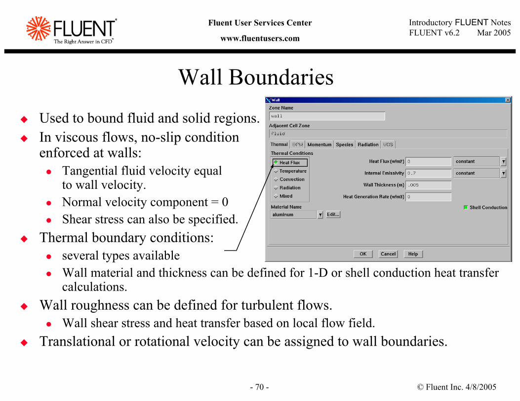
Wall Boundaries

Used to bound fluid and solid regions.In viscous flows, no-slip condition enforced at walls:

Tangential fluid velocity equalto wall velocity.Normal velocity component = 0Shear stress can also be specified.

Thermal boundary conditions:several types availableWall material and thickness can be defined for 1-D or shell conduction heat transfer calculations.

Wall roughness can be defined for turbulent flows.Wall shear stress and heat transfer based on local flow field.

Translational or rotational velocity can be assigned to wall boundaries.

© Fluent Inc. 4/8/2005- 71 -



www.fluentusers.com

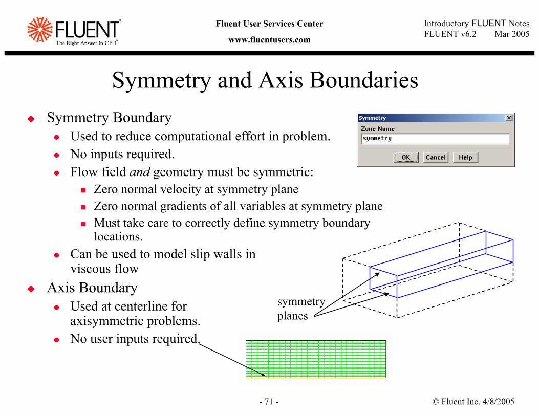
Symmetry and Axis BoundariesSymmetry Boundary

Used to reduce computational effort in problem.No inputs required.Flow field and geometry must be symmetric:

Zero normal velocity at symmetry planeZero normal gradients of all variables at symmetry planeMust take care to correctly define symmetry boundary locations.

Can be used to model slip walls in viscous flow

Axis BoundaryUsed at centerline for axisymmetric problems.No user inputs required.

symmetry planes

© Fluent Inc. 4/8/2005- 72 -



www.fluentusers.com

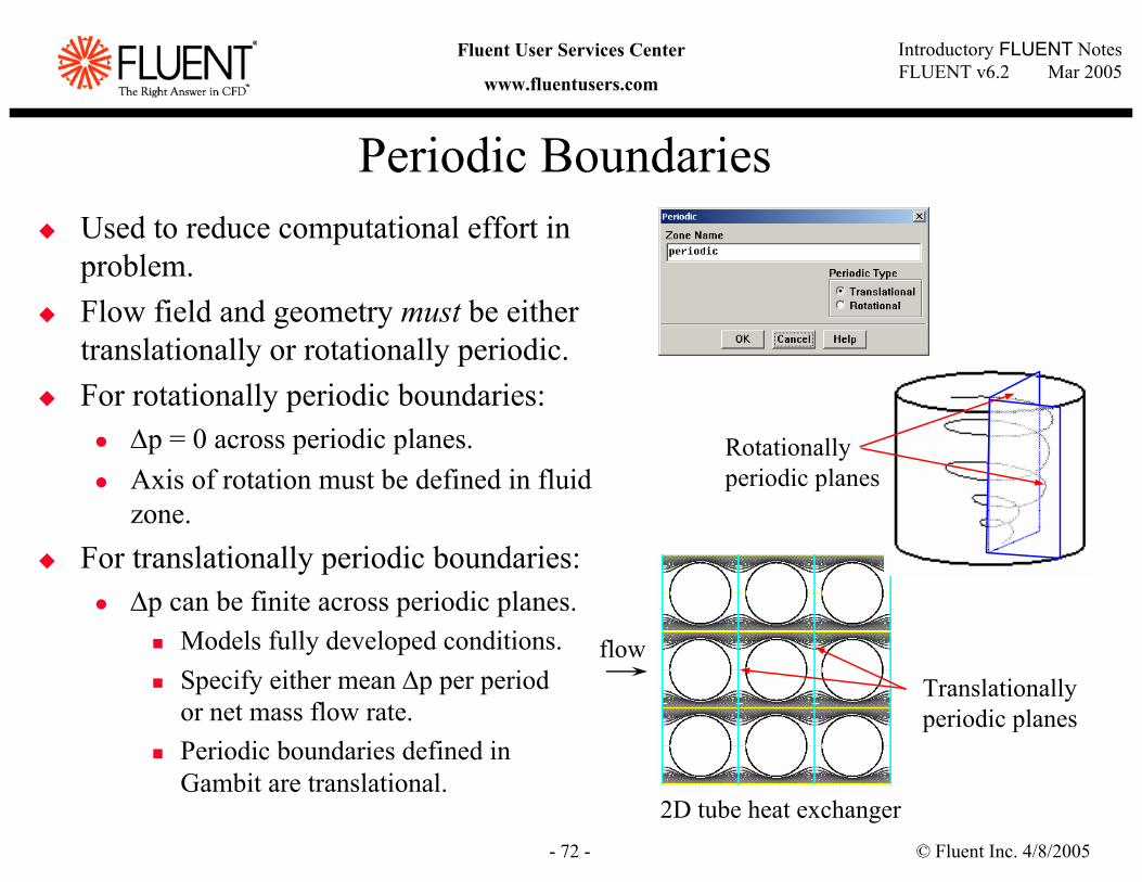
Periodic BoundariesUsed to reduce computational effort in problem.Flow field and geometry must be either translationally or rotationally periodic.For rotationally periodic boundaries:

∆p = 0 across periodic planes.Axis of rotation must be defined in fluid zone.

For translationally periodic boundaries:∆p can be finite across periodic planes.

Models fully developed conditions.Specify either mean ∆p per period or net mass flow rate.Periodic boundaries defined in Gambit are translational.

Translationallyperiodic planes

2D tube heat exchanger

flow

Rotationally periodic planes

© Fluent Inc. 4/8/2005- 73 -



www.fluentusers.com

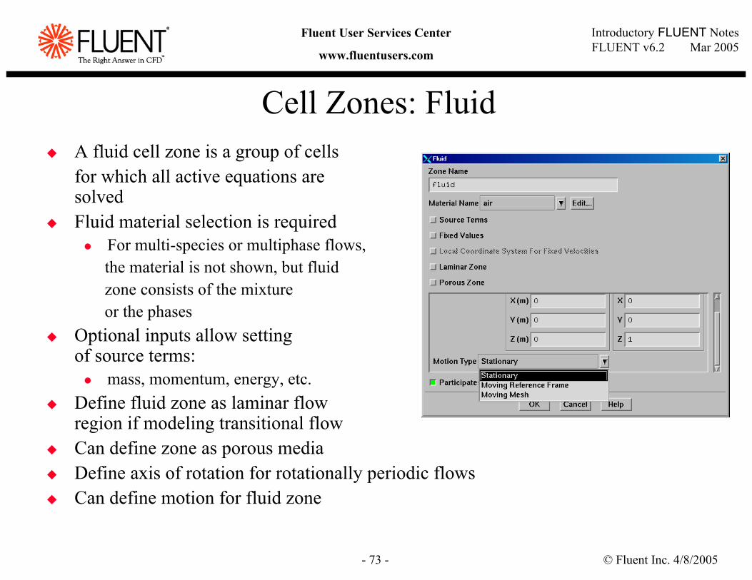
Cell Zones: FluidA fluid cell zone is a group of cellsfor which all active equations are solvedFluid material selection is required

For multi-species or multiphase flows,the material is not shown, but fluidzone consists of the mixtureor the phases

Optional inputs allow setting of source terms:

mass, momentum, energy, etc.Define fluid zone as laminar flow region if modeling transitional flowCan define zone as porous mediaDefine axis of rotation for rotationally periodic flowsCan define motion for fluid zone

© Fluent Inc. 4/8/2005- 74 -



www.fluentusers.com

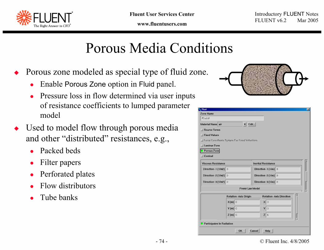
Porous Media ConditionsPorous zone modeled as special type of fluid zone.

Enable Porous Zone option in Fluid panel.Pressure loss in flow determined via user inputsof resistance coefficients to lumped parametermodel

Used to model flow through porous mediaand other “distributed” resistances, e.g.,

Packed bedsFilter papersPerforated platesFlow distributorsTube banks

© Fluent Inc. 4/8/2005- 75 -



www.fluentusers.com

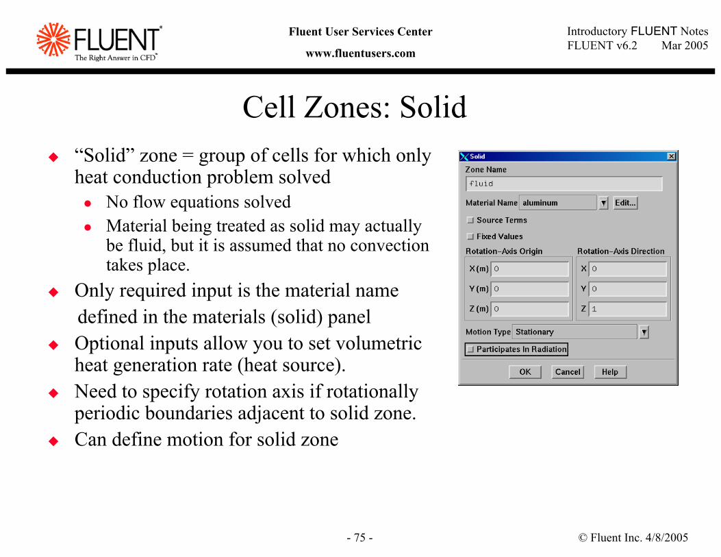
Cell Zones: Solid“Solid” zone = group of cells for which only heat conduction problem solved

No flow equations solvedMaterial being treated as solid may actually be fluid, but it is assumed that no convection takes place.

Only required input is the material namedefined in the materials (solid) panel Optional inputs allow you to set volumetric heat generation rate (heat source).Need to specify rotation axis if rotationally periodic boundaries adjacent to solid zone.Can define motion for solid zone

© Fluent Inc. 4/8/2005- 76 -



www.fluentusers.com

Internal Face Boundaries

Defined on the cell faces only:Thickness of these internal faces is zeroThese internal faces provide means of introducing step changes in flow properties.

Used to implement various physical models including:FansRadiatorsPorous-jump models

Preferable over porous media for its better convergence behavior.Interior walls

© Fluent Inc. 4/8/2005- 77 -



www.fluentusers.com

Summary

Zones are used to assign boundary conditions.Wide range of boundary conditions permit flow to enter and exit the solution domain.Wall boundary conditions are used to bound fluid and solid regions.Periodic boundaries are used to reduce computational effort.Internal cell zones are used to specify fluid, solid, and porous regions and heat-exchanger models.Internal face boundaries provide way to introduce step-changes in flow properties.

© Fluent Inc. 4/8/2005- 78 -



www.fluentusers.com

Solver Settings

© Fluent Inc. 4/8/2005- 79 -



www.fluentusers.com

OutlineUsing the Solver

Setting Solver ParametersConvergence

DefinitionMonitoringStabilityAccelerating Convergence

AccuracyGrid IndependenceGrid Adaption

Unsteady Flows ModelingUnsteady-flow problem setupNon-iterative Transient Advancement (NITA) schemesUnsteady flow modeling options

SummaryAppendix

© Fluent Inc. 4/8/2005- 80 -



www.fluentusers.com

OutlineUsing the Solver (solution procedure overview)





SummaryAppendix

© Fluent Inc. 4/8/2005- 81 -



www.fluentusers.com

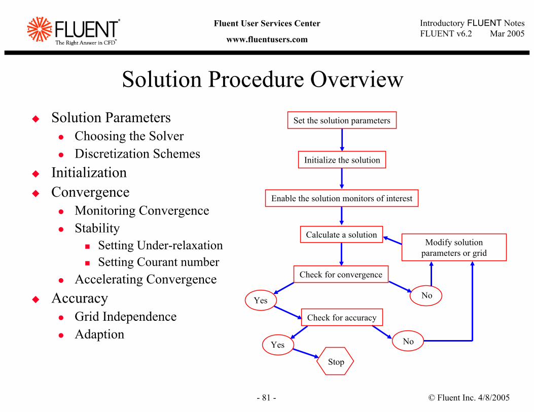
Modify solution parameters or grid

NoYes

No

Set the solution parameters

Initialize the solution

Enable the solution monitors of interest

Calculate a solution

Check for convergence

Check for accuracy

Stop

Yes

Solution Procedure OverviewSolution Parameters

Choosing the SolverDiscretization Schemes

InitializationConvergence

Monitoring ConvergenceStability

Setting Under-relaxationSetting Courant number

Accelerating ConvergenceAccuracy

Grid IndependenceAdaption

© Fluent Inc. 4/8/2005- 82 -



www.fluentusers.com

Choosing a SolverChoices are Coupled-Implicit, Coupled-Explicit, or Segregated (Implicit)The coupled solvers are recommended if a strong inter-dependence exists between density, energy, momentum, and/or species

e.g., high speed compressible flow or finite-rate reaction flowsIn general, the coupled-implicit solver is recommended over the coupled-explicit solver

Time required: Implicit solver runs roughly twice as fastMemory required: Implicit solver requires roughly twice as much memory as coupled-explicit or segregated solvers!Improved pre-conditioning in Fluent v6.2 for the coupled-implicit solver enhances accuracy and robustness for low-Mach number flows

The coupled-explicit solver should only be used for unsteady flows when the characteristic time scale of problem is on same order as that of the acoustics

e.g., tracking transient shock waveThe segregated (implicit) solver is preferred in all other cases.

Lower memory requirements than coupled-implicit solverSegregated approach provides flexibility in solution procedure

© Fluent Inc. 4/8/2005- 83 -



www.fluentusers.com

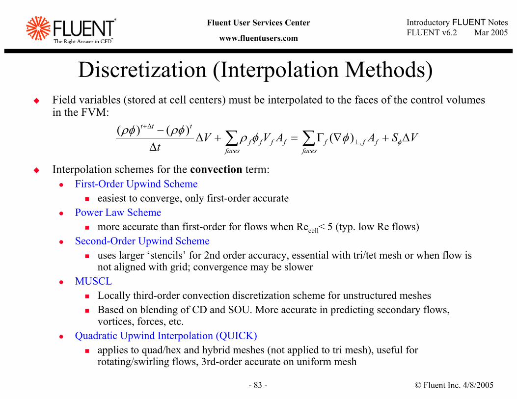
Discretization (Interpolation Methods)Field variables (stored at cell centers) must be interpolated to the faces of the control volumes in the FVM:

Interpolation schemes for the convection term:First-Order Upwind Scheme

easiest to converge, only first-order accuratePower Law Scheme

more accurate than first-order for flows when Recell< 5 (typ. low Re flows)Second-Order Upwind Scheme

uses larger ‘stencils’ for 2nd order accuracy, essential with tri/tet mesh or when flow is not aligned with grid; convergence may be slower

MUSCLLocally third-order convection discretization scheme for unstructured meshes Based on blending of CD and SOU. More accurate in predicting secondary flows, vortices, forces, etc.

Quadratic Upwind Interpolation (QUICK)applies to quad/hex and hybrid meshes (not applied to tri mesh), useful for rotating/swirling flows, 3rd-order accurate on uniform mesh

VSAAVVt f

facesfff

facesfff

ttt

∆+∇Γ=+∆∆

− ∑∑ ⊥

∆+

φφφρρφρφ,)()()(

© Fluent Inc. 4/8/2005- 84 -



www.fluentusers.com

Interpolation Methods for Face PressureInterpolation schemes for calculating cell-face pressures when using the segregated solver in FLUENT are available as follows:

Standarddefault scheme; reduced accuracy for flows exhibiting large surface-normal pressure gradients near boundaries (but should not be used when steep pressure changes are present in the flow - PRESTO! scheme should be used )

Linearuse when other options result in convergence difficulties or unphysical behavior.

Second-Orderuse for compressible flows; not to be used with porous media, jump, fans, etc. or VOF/Mixture multiphase models.

Body Force Weighteduse when body forces are large, e.g., high Ra natural convection or highly swirling flows.

PRESTO!use for highly swirling flows, flows involving steep pressure gradients (porous media, fan model, etc.), or in strongly curved domains.

© Fluent Inc. 4/8/2005- 85 -



www.fluentusers.com

Pressure-Velocity Coupling

Pressure-Velocity Coupling refers to the numerical algorithm which uses a combination of continuity and momentum equations to derive an equation for pressure (or pressure correction) when using the segregated solverThree algorithms available in FLUENT:

SIMPLEdefault scheme, robust

SIMPLECAllows faster convergence for simple problems (e.g., laminar flows with no physical models employed).

PISOuseful for unsteady flow problems or for meshes containing cells with higher than average skewness

© Fluent Inc. 4/8/2005- 86 -



www.fluentusers.com

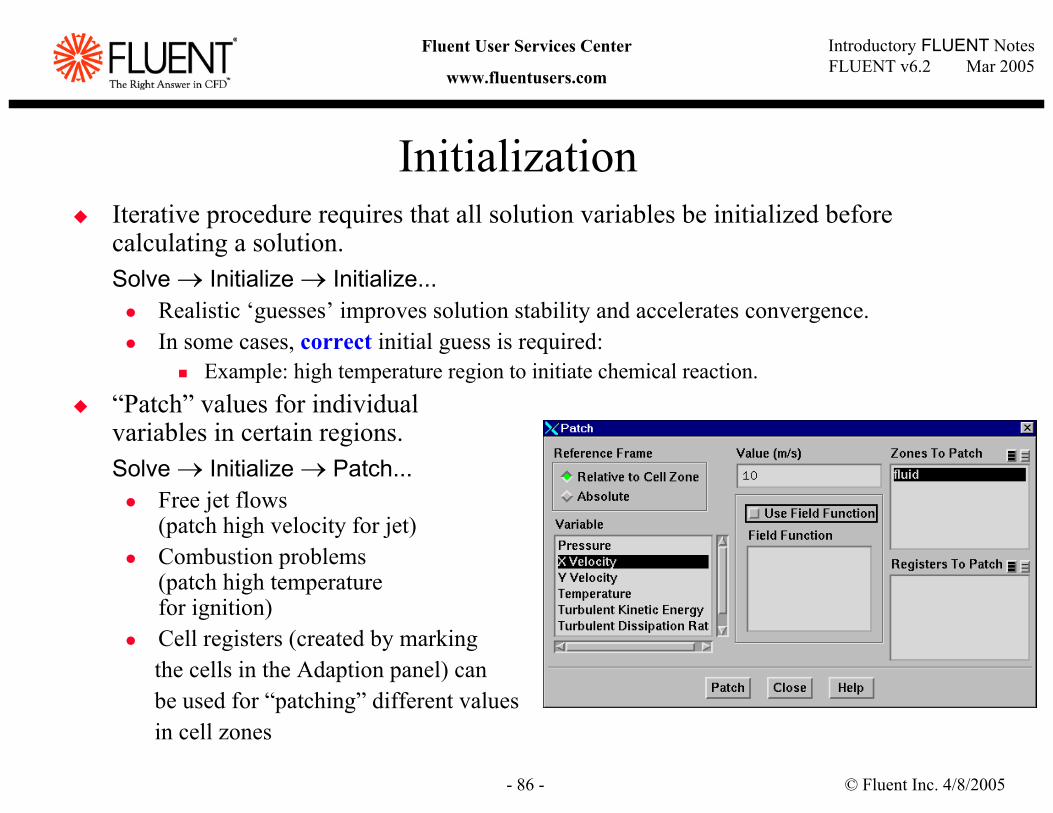
InitializationIterative procedure requires that all solution variables be initialized before calculating a solution.Solve → Initialize → Initialize...

Realistic ‘guesses’ improves solution stability and accelerates convergence.In some cases, correct initial guess is required:

Example: high temperature region to initiate chemical reaction.“Patch” values for individualvariables in certain regions.Solve → Initialize → Patch...

Free jet flows(patch high velocity for jet)Combustion problems(patch high temperaturefor ignition)Cell registers (created by marking the cells in the Adaption panel) can be used for “patching” different values in cell zones

© Fluent Inc. 4/8/2005- 87 -



www.fluentusers.com






SummaryAppendix

© Fluent Inc. 4/8/2005- 88 -



www.fluentusers.com

ConvergenceAt convergence:

All discrete conservation equations (momentum, energy, etc.) areobeyed in all cells to a specified tolerance.Solution no longer changes with more iterations.Overall mass, momentum, energy, and scalar balances are achieved.

Monitoring convergence with residuals’ history:Generally, a decrease in residuals by 3 orders of magnitude indicates at least qualitative convergence.

Major flow features established.Scaled energy residual must decrease to 10-6 for segregated solver.Scaled species residual may need to decrease to 10-5 to achieve species balance.

Monitoring quantitative convergence:Monitor other relevant key variables/physical quantities for a confirmation.Ensure that property conservation is satisfied.

© Fluent Inc. 4/8/2005- 89 -



www.fluentusers.com

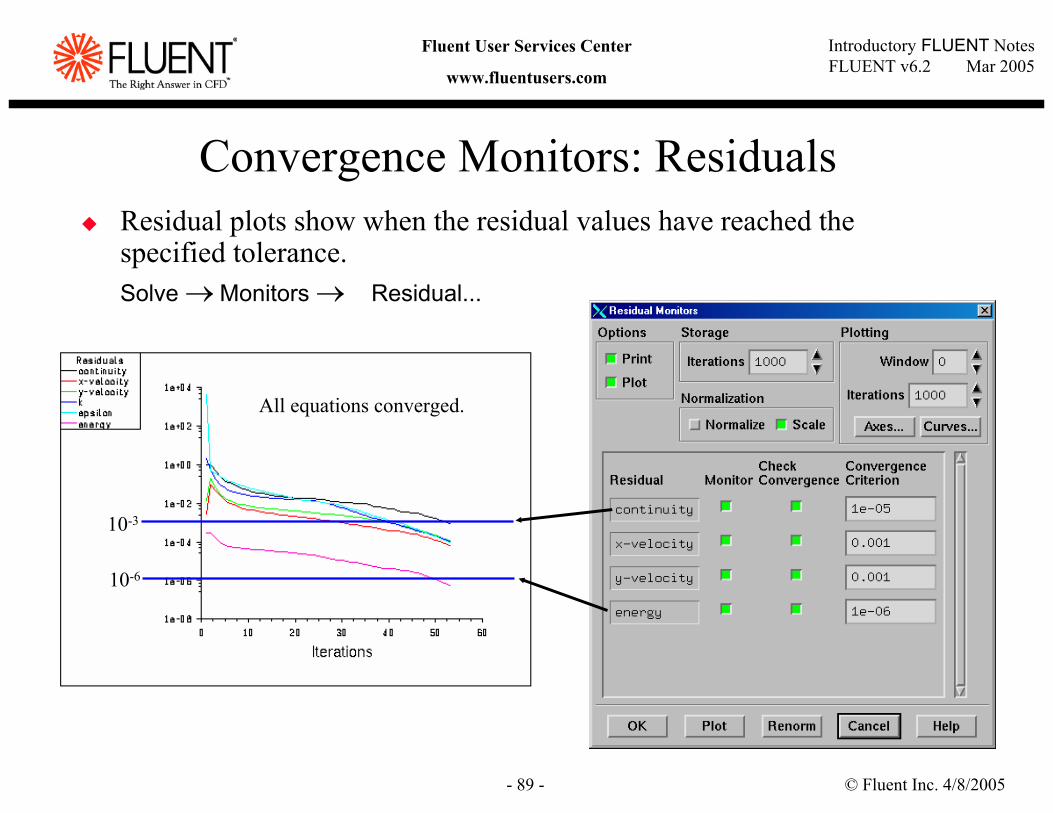
Convergence Monitors: ResidualsResidual plots show when the residual values have reached the specified tolerance.Solve → Monitors → Residual...

All equations converged.

10-3

10-6

© Fluent Inc. 4/8/2005- 90 -



www.fluentusers.com

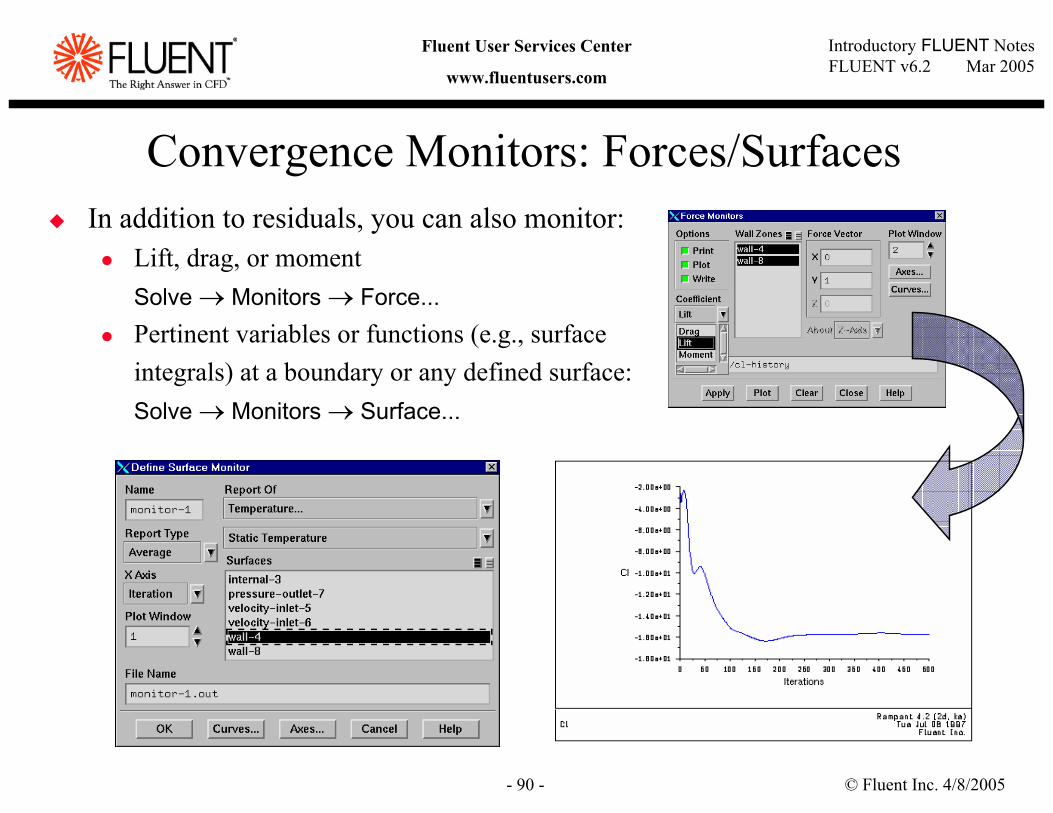
Convergence Monitors: Forces/SurfacesIn addition to residuals, you can also monitor:

Lift, drag, or momentSolve → Monitors → Force... Pertinent variables or functions (e.g., surface integrals) at a boundary or any defined surface: Solve → Monitors → Surface...

© Fluent Inc. 4/8/2005- 91 -



www.fluentusers.com

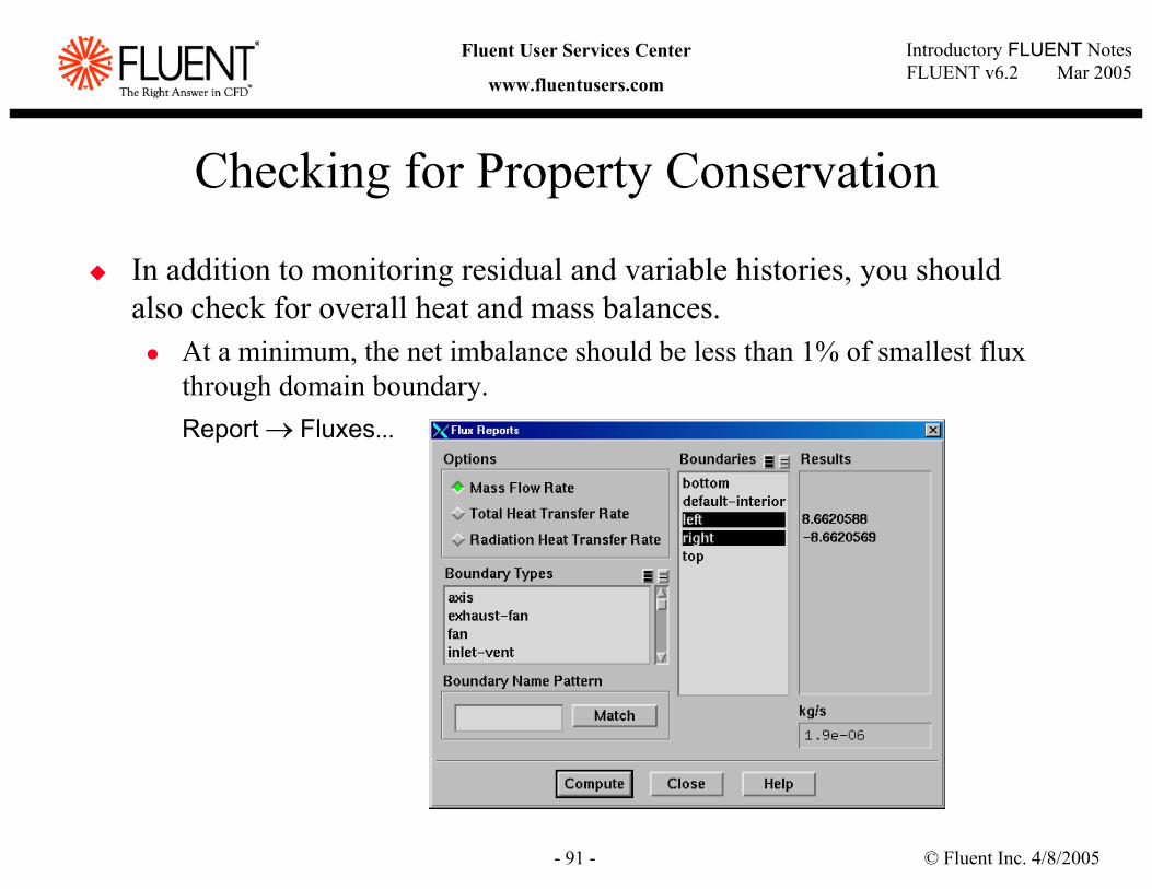
Checking for Property Conservation

In addition to monitoring residual and variable histories, you should also check for overall heat and mass balances.

At a minimum, the net imbalance should be less than 1% of smallest flux through domain boundary.Report → Fluxes...

© Fluent Inc. 4/8/2005- 92 -



www.fluentusers.com

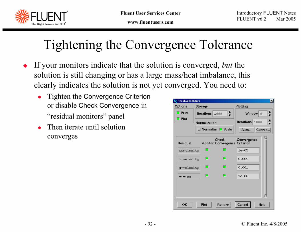
Tightening the Convergence ToleranceIf your monitors indicate that the solution is converged, but the solution is still changing or has a large mass/heat imbalance, this clearly indicates the solution is not yet converged. You need to:

Tighten the Convergence Criterionor disable Check Convergence in “residual monitors” panelThen iterate until solutionconverges

© Fluent Inc. 4/8/2005- 93 -



www.fluentusers.com

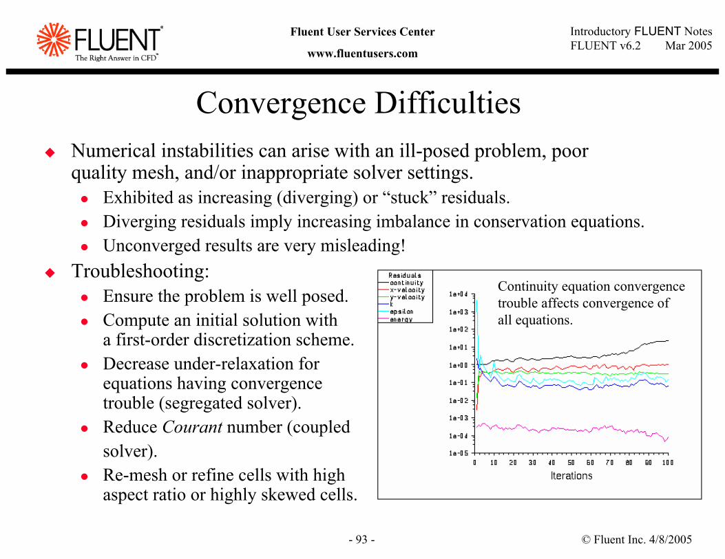
Convergence DifficultiesNumerical instabilities can arise with an ill-posed problem, poor quality mesh, and/or inappropriate solver settings.

Exhibited as increasing (diverging) or “stuck” residuals.Diverging residuals imply increasing imbalance in conservation equations.Unconverged results are very misleading!

Troubleshooting:Ensure the problem is well posed.Compute an initial solution witha first-order discretization scheme.Decrease under-relaxation for equations having convergence trouble (segregated solver).Reduce Courant number (coupled solver).Re-mesh or refine cells with high aspect ratio or highly skewed cells.

Continuity equation convergencetrouble affects convergence ofall equations.

© Fluent Inc. 4/8/2005- 94 -



www.fluentusers.com

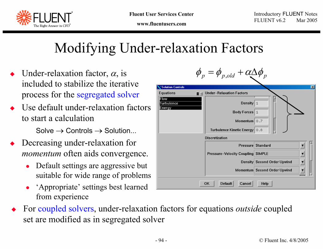
Modifying Under-relaxation Factors

Under-relaxation factor, α, is included to stabilize the iterative process for the segregated solverUse default under-relaxation factors to start a calculation

Solve → Controls → Solution...

Decreasing under-relaxation for momentum often aids convergence.

Default settings are aggressive but suitable for wide range of problems‘Appropriate’ settings best learned from experience

poldpp φαφφ ∆+= ,

For coupled solvers, under-relaxation factors for equations outside coupled set are modified as in segregated solver

© Fluent Inc. 4/8/2005- 95 -



www.fluentusers.com

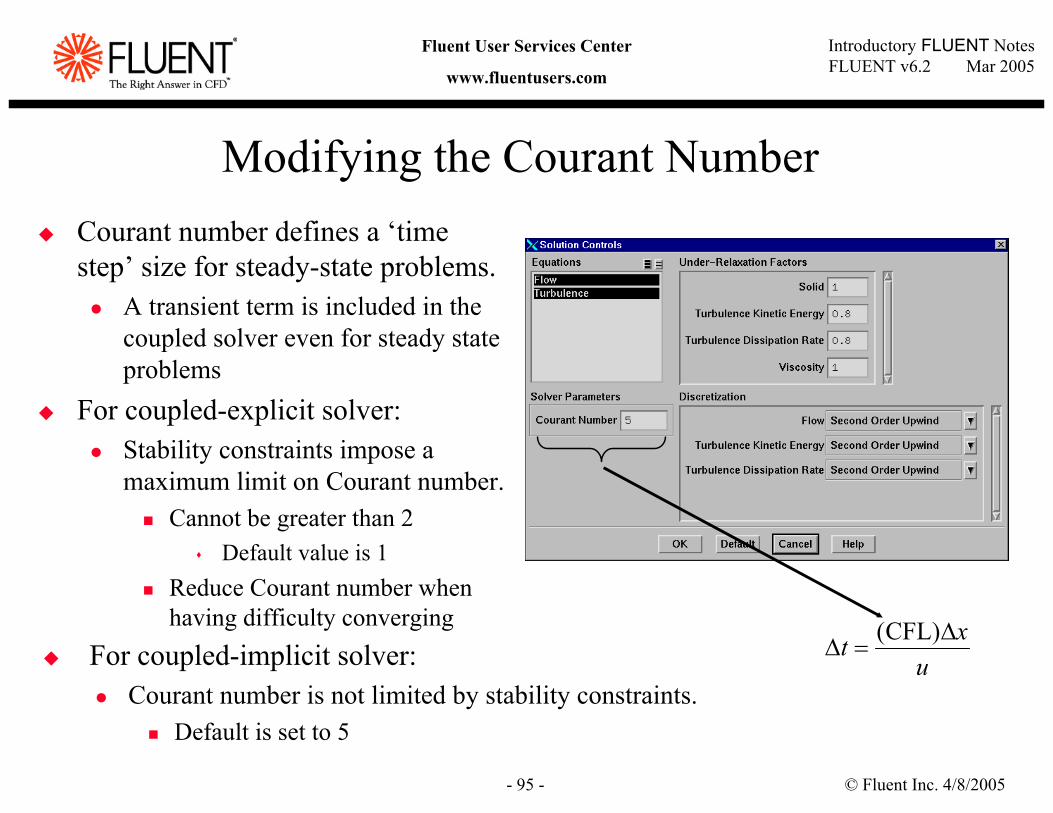
Modifying the Courant NumberCourant number defines a ‘time step’ size for steady-state problems.

A transient term is included in the coupled solver even for steady state problems

For coupled-explicit solver:Stability constraints impose a maximum limit on Courant number.

Cannot be greater than 2Default value is 1

Reduce Courant number when having difficulty converging

uxt ∆

=∆)CFL(

For coupled-implicit solver:Courant number is not limited by stability constraints.

Default is set to 5

© Fluent Inc. 4/8/2005- 96 -



www.fluentusers.com

Accelerating Convergence

Convergence can be accelerated by:Supplying good initial conditions

Starting from a previous solutionIncreasing under-relaxation factors or Courant number

Excessively high values can lead to instabilitiesRecommend saving case and data files before continuing iterations.

Controlling multigrid solver settingsDefault settings define robust Multigrid solver and typically do not need to be changed

© Fluent Inc. 4/8/2005- 97 -



www.fluentusers.com

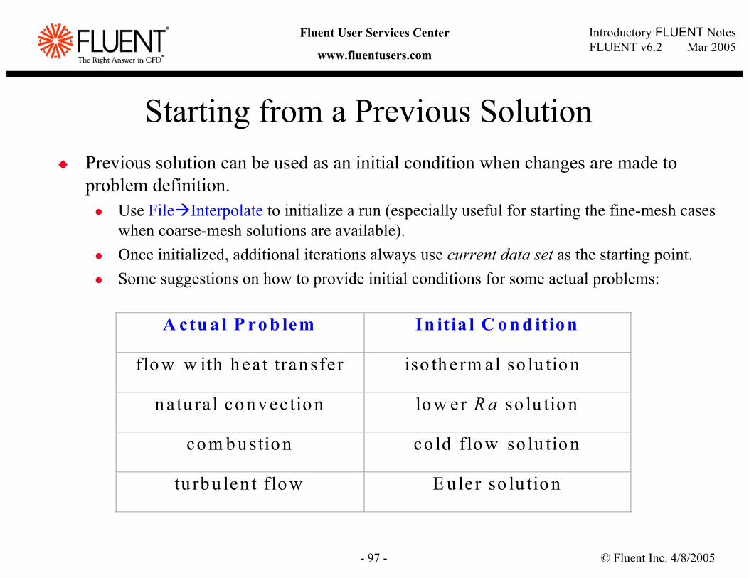
Starting from a Previous SolutionPrevious solution can be used as an initial condition when changes are made to problem definition.

Use File Interpolate to initialize a run (especially useful for starting the fine-mesh cases when coarse-mesh solutions are available).Once initialized, additional iterations always use current data set as the starting point.Some suggestions on how to provide initial conditions for some actual problems:

A ctu a l P ro b lem In itia l C o n d itio n

flo w w ith h eat tran sfer iso th erm al so lu tio n

n atu ra l co n v ec tio n lo w er R a so lu tio n

co m b u stio n co ld flo w so lu tio n

tu rb u len t flo w E u ler so lu tio n

© Fluent Inc. 4/8/2005- 98 -



www.fluentusers.com

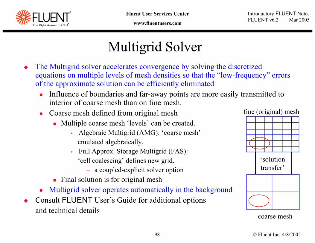
Multigrid SolverThe Multigrid solver accelerates convergence by solving the discretizedequations on multiple levels of mesh densities so that the “low-frequency” errors of the approximate solution can be efficiently eliminated

Influence of boundaries and far-away points are more easily transmitted to interior of coarse mesh than on fine mesh.Coarse mesh defined from original mesh

Multiple coarse mesh ‘levels’ can be created.Algebraic Multigrid (AMG): ‘coarse mesh’emulated algebraically.Full Approx. Storage Multigrid (FAS):‘cell coalescing’ defines new grid.

– a coupled-explicit solver optionFinal solution is for original mesh

Multigrid solver operates automatically in the backgroundConsult FLUENT User’s Guide for additional options and technical details

fine (original) mesh

coarse mesh

‘solution transfer’

© Fluent Inc. 4/8/2005- 99 -



www.fluentusers.com






SummaryAppendix

© Fluent Inc. 4/8/2005- 100 -



www.fluentusers.com

Solution Accuracy

A converged solution is not necessarily a correct one!Always inspect and evaluate the solution by using available data, physical principles and so on. Use the second-order upwind discretization scheme for final results.Ensure that solution is grid-independent:

Use adaption to modify the grid or create additional meshes for the grid-independence study

If flow features do not seem reasonable:Reconsider physical models and boundary conditionsExamine mesh quality and possibly re-mesh the problemReconsider the choice of the boundaries’ location (or the domain): inadequate choice of domain (especially the outlet boundary) cansignificantly impact solution accuracy

© Fluent Inc. 4/8/2005- 101 -



www.fluentusers.com

Mesh Quality and Solution AccuracyNumerical errors are associated with calculation of cell gradients and cell face interpolations.Ways to contain the numerical errors:

Use higher-order discretization schemes (second-order upwind, MUSCL)Attempt to align grid with the flow to minimize the “false diffusion”Refine the mesh

Sufficient mesh density is necessary to resolve salient features of flowInterpolation errors decrease with decreasing cell size

Minimize variations in cell size in non-uniform meshesTruncation error is minimized in a uniform meshFLUENT provides capability to adapt mesh based on cell size variation

Minimize cell skewness and aspect ratioIn general, avoid aspect ratios higher than 5:1 (but higher ratios are allowed in boundary layers)Optimal quad/hex cells have bounded angles of 90 degreesOptimal tri/tet cells are equilateral

© Fluent Inc. 4/8/2005- 102 -



www.fluentusers.com

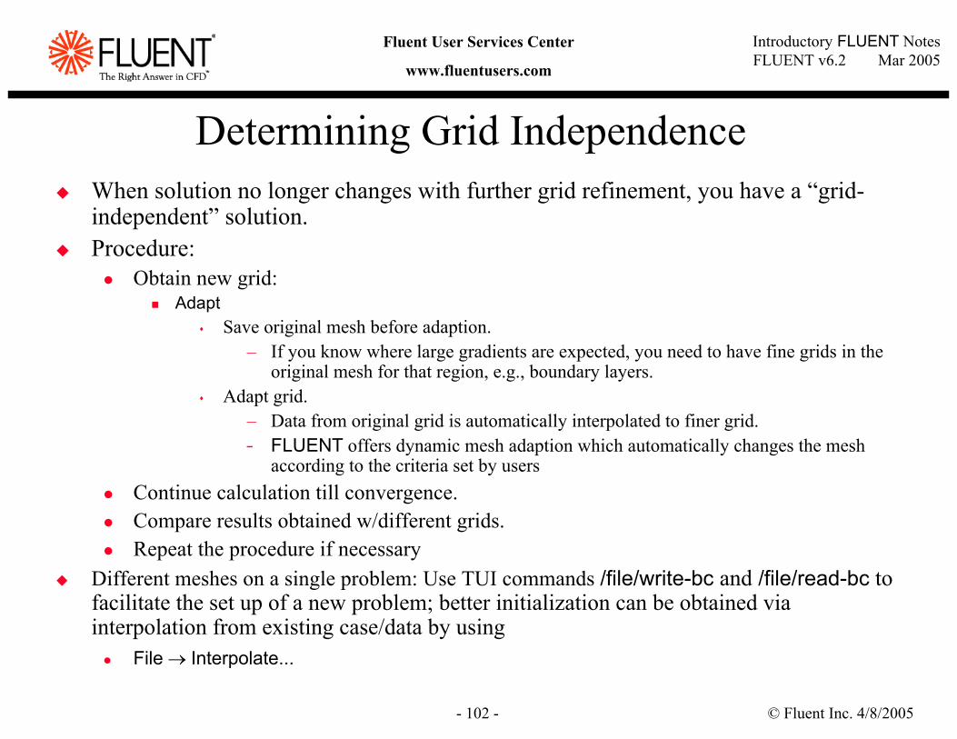
Determining Grid IndependenceWhen solution no longer changes with further grid refinement, you have a “grid-independent” solution.Procedure:

Obtain new grid:Adapt

Save original mesh before adaption.– If you know where large gradients are expected, you need to have fine grids in the

original mesh for that region, e.g., boundary layers. Adapt grid.

– Data from original grid is automatically interpolated to finer grid.– FLUENT offers dynamic mesh adaption which automatically changes the mesh

according to the criteria set by users Continue calculation till convergence.Compare results obtained w/different grids.Repeat the procedure if necessary

Different meshes on a single problem: Use TUI commands /file/write-bc and /file/read-bc to facilitate the set up of a new problem; better initialization can be obtained via interpolation from existing case/data by using

File → Interpolate...

© Fluent Inc. 4/8/2005- 103 -



www.fluentusers.com






SummaryAppendix

© Fluent Inc. 4/8/2005- 104 -



www.fluentusers.com

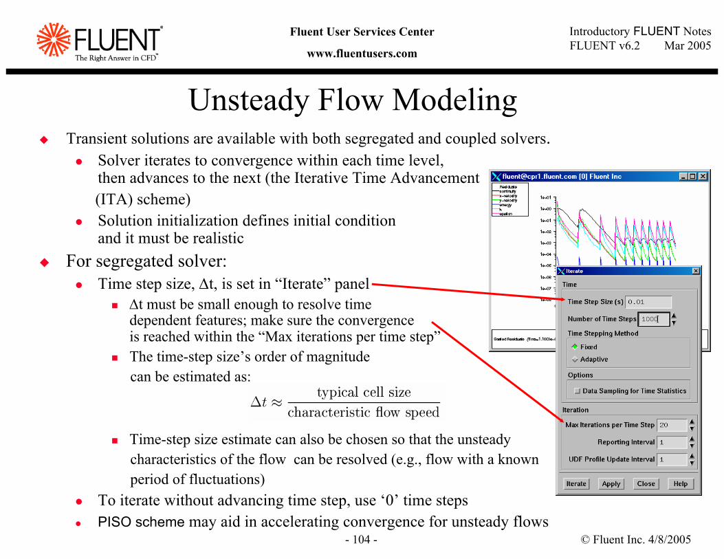
Unsteady Flow ModelingTransient solutions are available with both segregated and coupled solvers.

Solver iterates to convergence within each time level, then advances to the next (the Iterative Time Advancement(ITA) scheme)Solution initialization defines initial condition and it must be realistic

For segregated solver:Time step size, ∆t, is set in “Iterate” panel

∆t must be small enough to resolve time dependent features; make sure the convergence is reached within the “Max iterations per time step”The time-step size’s order of magnitude can be estimated as:

Time-step size estimate can also be chosen so that the unsteady characteristics of the flow can be resolved (e.g., flow with a knownperiod of fluctuations)

To iterate without advancing time step, use ‘0’ time stepsPISO scheme may aid in accelerating convergence for unsteady flows

© Fluent Inc. 4/8/2005- 105 -



www.fluentusers.com

NITA Schemes for the Segregated Solver

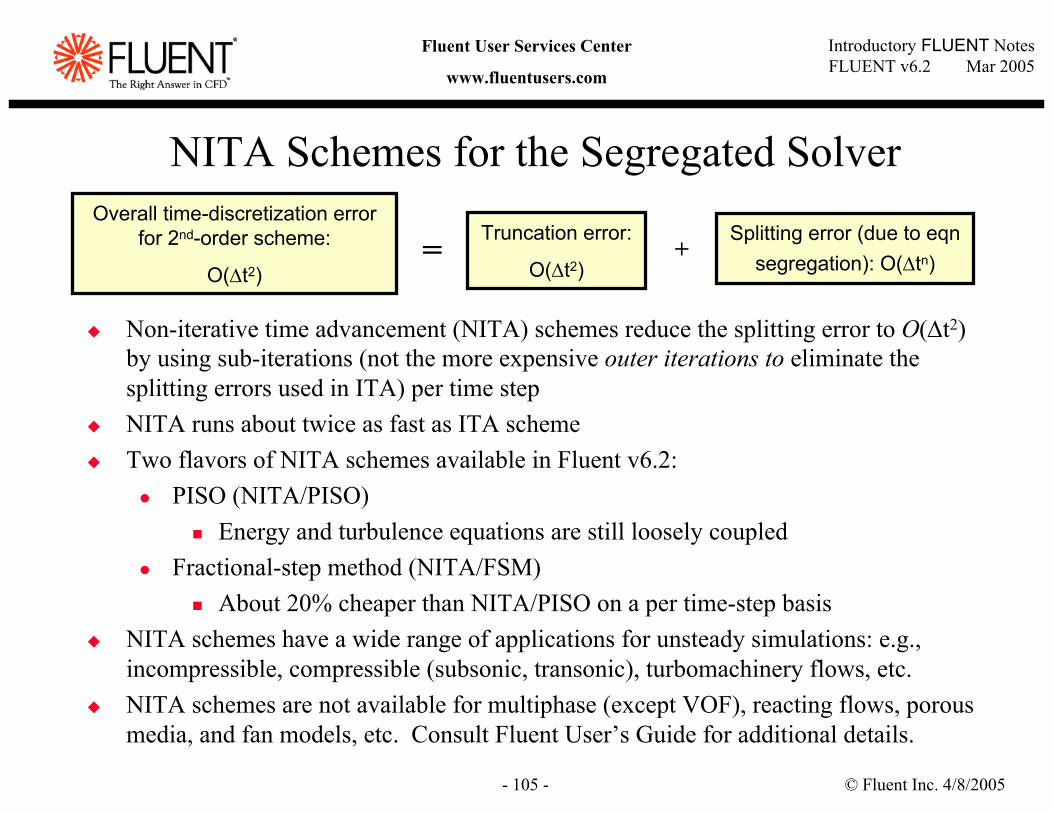
Non-iterative time advancement (NITA) schemes reduce the splitting error to O(∆t2) by using sub-iterations (not the more expensive outer iterations to eliminate the splitting errors used in ITA) per time stepNITA runs about twice as fast as ITA schemeTwo flavors of NITA schemes available in Fluent v6.2:

PISO (NITA/PISO)Energy and turbulence equations are still loosely coupled

Fractional-step method (NITA/FSM)About 20% cheaper than NITA/PISO on a per time-step basis

NITA schemes have a wide range of applications for unsteady simulations: e.g., incompressible, compressible (subsonic, transonic), turbomachinery flows, etc.NITA schemes are not available for multiphase (except VOF), reacting flows, porous media, and fan models, etc. Consult Fluent User’s Guide for additional details.

Truncation error:

O(∆t2)

Splitting error (due to eqnsegregation): O(∆tn)

Overall time-discretization error for 2nd-order scheme:

O(∆t2)= +

© Fluent Inc. 4/8/2005- 106 -



www.fluentusers.com

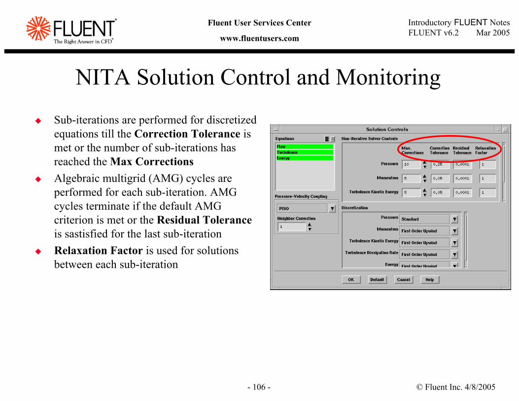
NITA Solution Control and Monitoring

Sub-iterations are performed for discretizedequations till the Correction Tolerance is met or the number of sub-iterations has reached the Max CorrectionsAlgebraic multigrid (AMG) cycles are performed for each sub-iteration. AMG cycles terminate if the default AMG criterion is met or the Residual Tolerance is sastisfied for the last sub-iterationRelaxation Factor is used for solutions between each sub-iteration

© Fluent Inc. 4/8/2005- 107 -



www.fluentusers.com

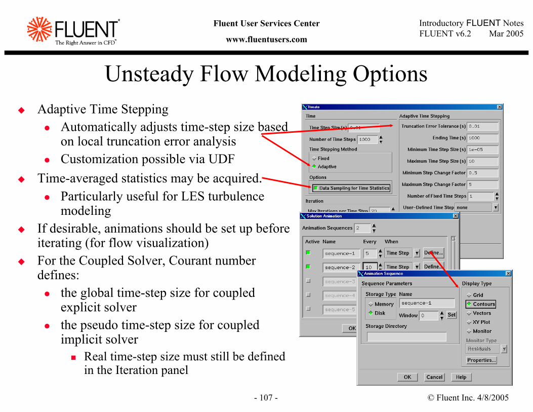
Unsteady Flow Modeling Options Adaptive Time Stepping

Automatically adjusts time-step size based on local truncation error analysisCustomization possible via UDF

Time-averaged statistics may be acquired.Particularly useful for LES turbulence modeling

If desirable, animations should be set up before iterating (for flow visualization)For the Coupled Solver, Courant number defines:

the global time-step size for coupled explicit solverthe pseudo time-step size for coupled implicit solver

Real time-step size must still be defined in the Iteration panel

© Fluent Inc. 4/8/2005- 108 -



www.fluentusers.com

Summary

Solution procedure for the segregated and coupled solvers is the same:Calculate until you get a converged solutionObtain second-order solution (recommended)Refine grid and recalculate until grid-independent solution is obtained

All solvers provide tools for judging and improving convergence and ensuring stabilityAll solvers provide tools for checking and improving accuracySolution accuracy will depend on the appropriateness of the physical models that you choose and the boundary conditions that you specify.

© Fluent Inc. 4/8/2005- 109 -



www.fluentusers.com

Appendix

BackgroundFinite Volume MethodExplicit vs. ImplicitSegregated vs. CoupledTransient SolutionsFlow Diagrams of NITA and ITA Schemes

© Fluent Inc. 4/8/2005- 110 -



www.fluentusers.com

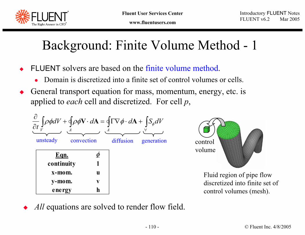
Background: Finite Volume Method - 1FLUENT solvers are based on the finite volume method.

Domain is discretized into a finite set of control volumes or cells.General transport equation for mass, momentum, energy, etc. is applied to each cell and discretized. For cell p,

∫∫∫∫∀

+⋅∇Γ=⋅+∂∂ dVSdddVt AAV

φφρφρφ AAV

unsteady convection diffusion generation

Eqn.continuity 1

x-mom. uy-mom. venergy h

φ

Fluid region of pipe flow discretized into finite set of control volumes (mesh).

control volume

All equations are solved to render flow field.

© Fluent Inc. 4/8/2005- 111 -



www.fluentusers.com

Background: Finite Volume Method - 2

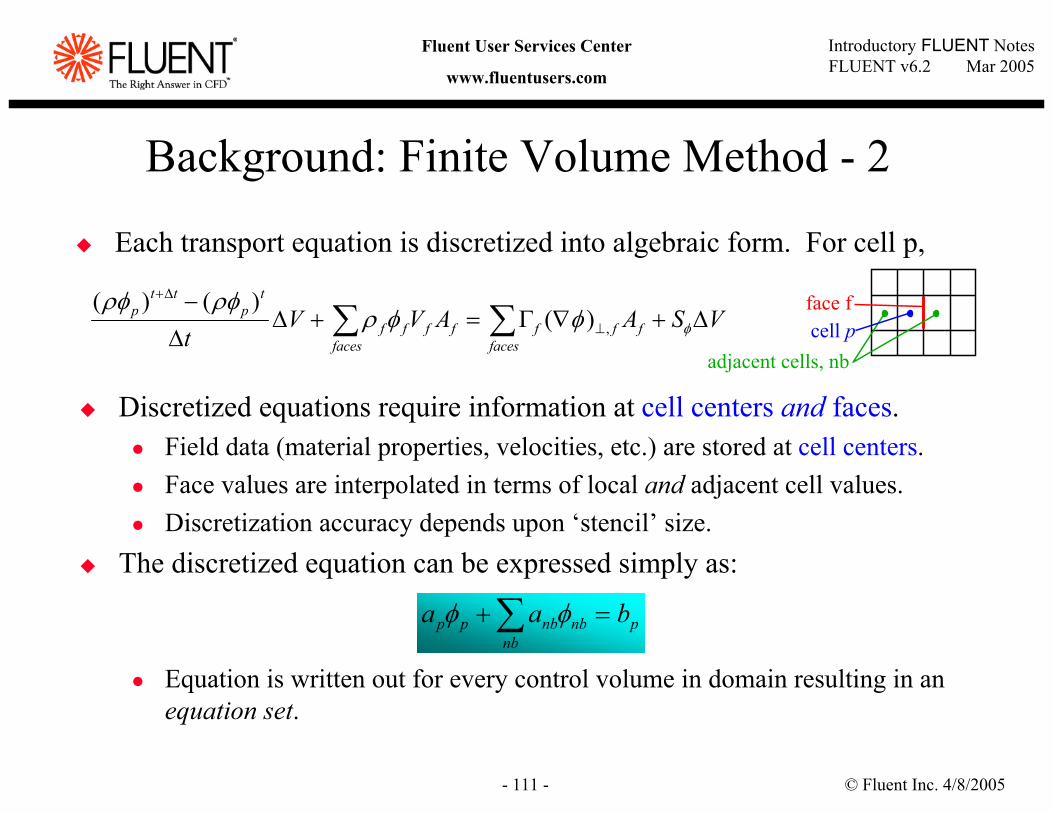
Each transport equation is discretized into algebraic form. For cell p,

face f

adjacent cells, nbcell p

Discretized equations require information at cell centers and faces.Field data (material properties, velocities, etc.) are stored at cell centers.Face values are interpolated in terms of local and adjacent cell values.Discretization accuracy depends upon ‘stencil’ size.

The discretized equation can be expressed simply as:

Equation is written out for every control volume in domain resulting in an equation set.

pnb

nbnbpp baa =+ ∑ φφ

VSAAVVt f

facesfff

facesfff

tp

ttp ∆+∇Γ=+∆

∆−

∑∑ ⊥

∆+

φφφρρφρφ

,)()()(

© Fluent Inc. 4/8/2005- 112 -



www.fluentusers.com

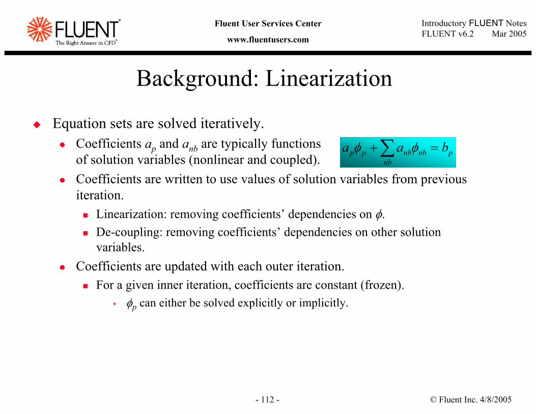
Equation sets are solved iteratively.Coefficients ap and anb are typically functions of solution variables (nonlinear and coupled).Coefficients are written to use values of solution variables from previous iteration.

Linearization: removing coefficients’ dependencies on φ.De-coupling: removing coefficients’ dependencies on other solution variables.

Coefficients are updated with each outer iteration.For a given inner iteration, coefficients are constant (frozen).

φp can either be solved explicitly or implicitly.

Background: Linearization

pnb


© Fluent Inc. 4/8/2005- 113 -



www.fluentusers.com

Assumptions are made about the knowledge of φnb:Explicit linearization - unknown value in each cell computed from relations that include only existing values (φnb assumed known from previous iteration).

φp solved explicitly using Runge-Kutta scheme.Implicit linearization - φp and φnb are assumed unknown and are solved using linear equation techniques.

Equations that are implicitly linearized tend to have less restrictive stability requirements.The equation set is solved simultaneously using a second iterative loop (e.g., point Gauss-Seidel).

Background: Explicit vs. Implicit

© Fluent Inc. 4/8/2005- 114 -



www.fluentusers.com

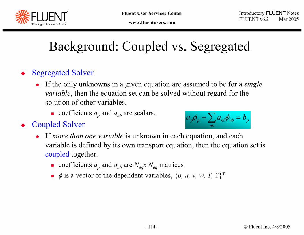
Background: Coupled vs. Segregated

Segregated SolverIf the only unknowns in a given equation are assumed to be for a single variable, then the equation set can be solved without regard for the solution of other variables.

coefficients ap and anb are scalars.

Coupled SolverIf more than one variable is unknown in each equation, and each variable is defined by its own transport equation, then the equation set is coupled together.

coefficients ap and anb are Neqx Neq matricesφ is a vector of the dependent variables, p, u, v, w, T, YT

pnb


© Fluent Inc. 4/8/2005- 115 -



www.fluentusers.com

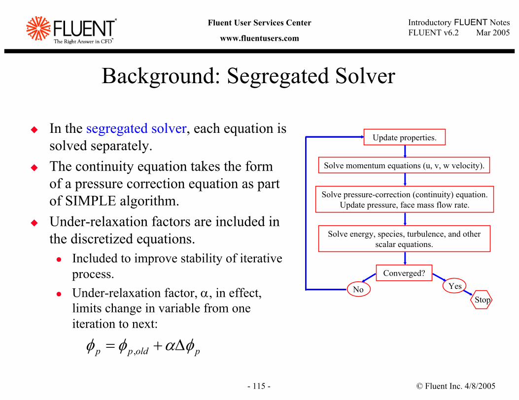
Background: Segregated Solver

In the segregated solver, each equation is solved separately.The continuity equation takes the form of a pressure correction equation as part of SIMPLE algorithm.Under-relaxation factors are included in the discretized equations.

Included to improve stability of iterative process.Under-relaxation factor, α, in effect, limits change in variable from one iteration to next:

Update properties.

Solve momentum equations (u, v, w velocity).

Solve pressure-correction (continuity) equation.Update pressure, face mass flow rate.

Solve energy, species, turbulence, and other scalar equations.

Converged?

StopNo Yes

poldpp φαφφ ∆+= ,

© Fluent Inc. 4/8/2005- 116 -



www.fluentusers.com

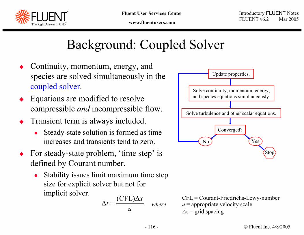
Background: Coupled SolverContinuity, momentum, energy, and species are solved simultaneously in the coupled solver.Equations are modified to resolve compressible and incompressible flow.Transient term is always included.

Steady-state solution is formed as time increases and transients tend to zero.

For steady-state problem, ‘time step’ is defined by Courant number.

Stability issues limit maximum time step size for explicit solver but not for implicit solver.

Solve continuity, momentum, energy, and species equations simultaneously.

Stop

No Yes

Solve turbulence and other scalar equations.

Update properties.

Converged?

uxt ∆

=∆)CFL( CFL = Courant-Friedrichs-Lewy-number

where u = appropriate velocity scale∆x = grid spacing

© Fluent Inc. 4/8/2005- 117 -



www.fluentusers.com

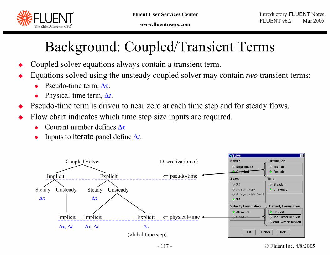
Background: Coupled/Transient Terms Coupled solver equations always contain a transient term.Equations solved using the unsteady coupled solver may contain two transient terms:

Pseudo-time term, ∆τ.Physical-time term, ∆t.

Pseudo-time term is driven to near zero at each time step and for steady flows.Flow chart indicates which time step size inputs are required.

Courant number defines ∆τInputs to Iterate panel define ∆t.

Coupled Solver

ExplicitImplicit

Steady Unsteady Steady Unsteady

∆τ, ∆t

∆τ

∆τ, ∆t

∆τ

∆τ

⇐ pseudo-time

ExplicitImplicit ⇐ physical-timeImplicit

Discretization of:

(global time step)

© Fluent Inc. 4/8/2005- 118 -



www.fluentusers.com

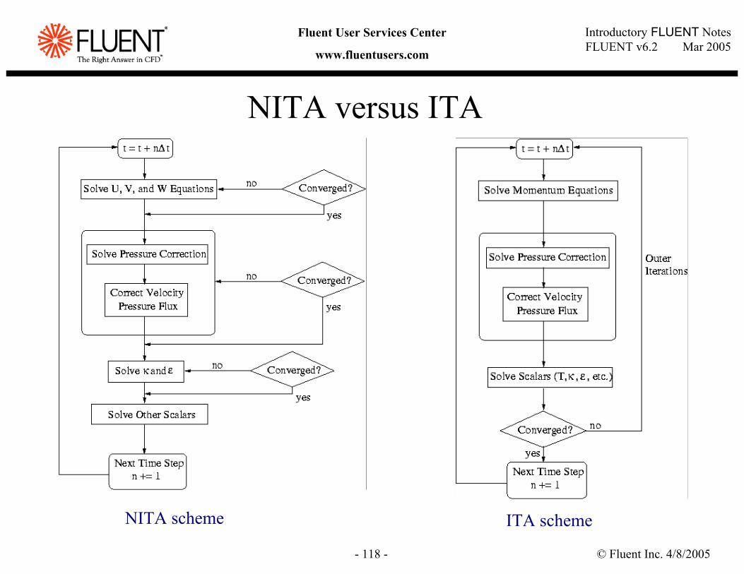
NITA versus ITA

NITA scheme ITA scheme

© Fluent Inc. 4/8/2005- 119 -



www.fluentusers.com

Modeling Turbulent Flows

© Fluent Inc. 4/8/2005- 120 -



www.fluentusers.com

What is Turbulence?Unsteady, irregular (aperiodic) motion in which transported quantities (mass, momentum, scalar species) fluctuate in time and space

Identifiable swirling patterns characterize turbulent eddies.Enhanced mixing (matter, momentum, energy, etc.) results

Fluid properties and velocity exhibit random variationsStatistical averaging results in accountable, turbulence related transport mechanisms.This characteristic allows for Turbulence Modeling.

Contains a wide range of turbulent eddy sizes (scales spectrum).The size/velocity of large eddies is on the order of mean flow.

Large eddies derive energy from the mean flowEnergy is transferred from larger eddies to smaller eddies

In the smallest eddies, turbulent energy is converted to internal energy by viscous dissipation.

© Fluent Inc. 4/8/2005- 121 -



www.fluentusers.com

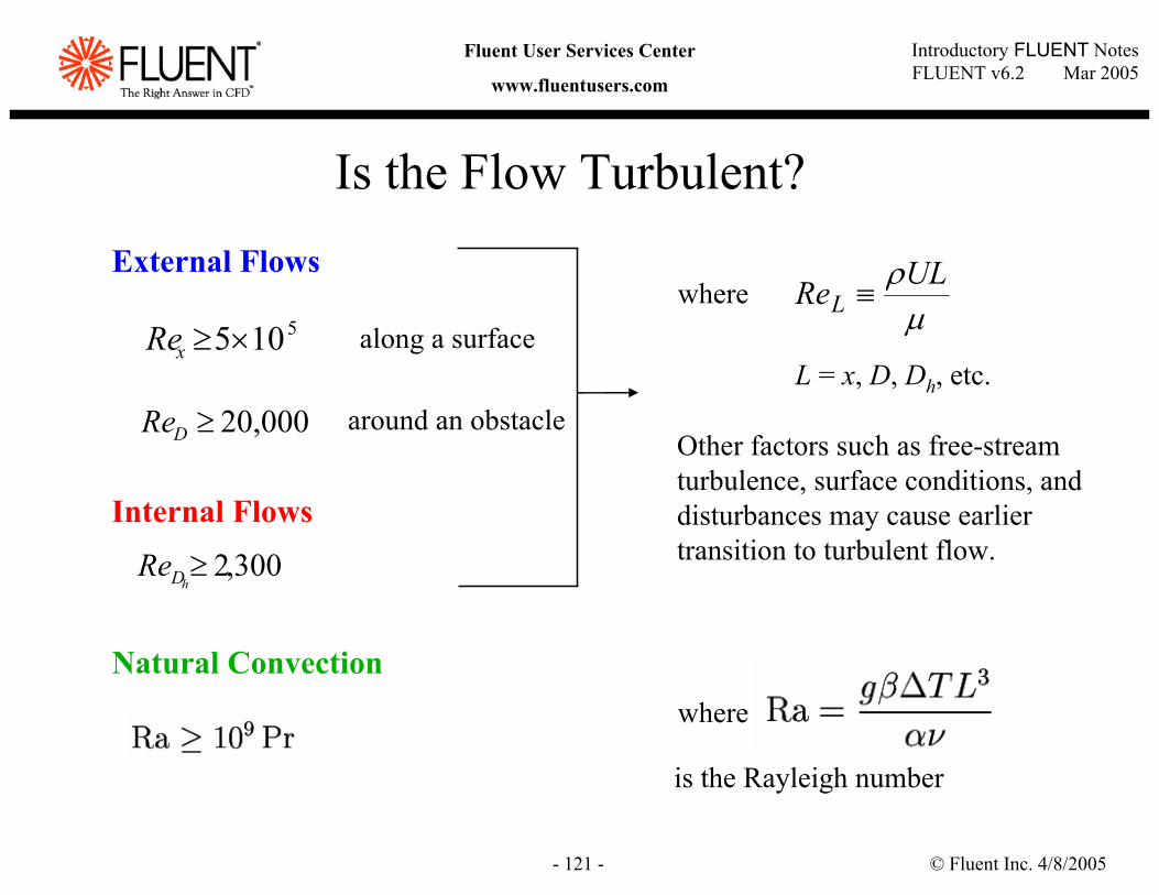
Is the Flow Turbulent?External Flows

Internal Flows

Natural Convection

5105×≥xRe along a surface

around an obstacle

where

µρULReL ≡where

Other factors such as free-stream turbulence, surface conditions, and disturbances may cause earlier transition to turbulent flow.

L = x, D, Dh, etc.

,3002 ≥hD Re

20,000≥DRe

is the Rayleigh number

© Fluent Inc. 4/8/2005- 122 -



www.fluentusers.com

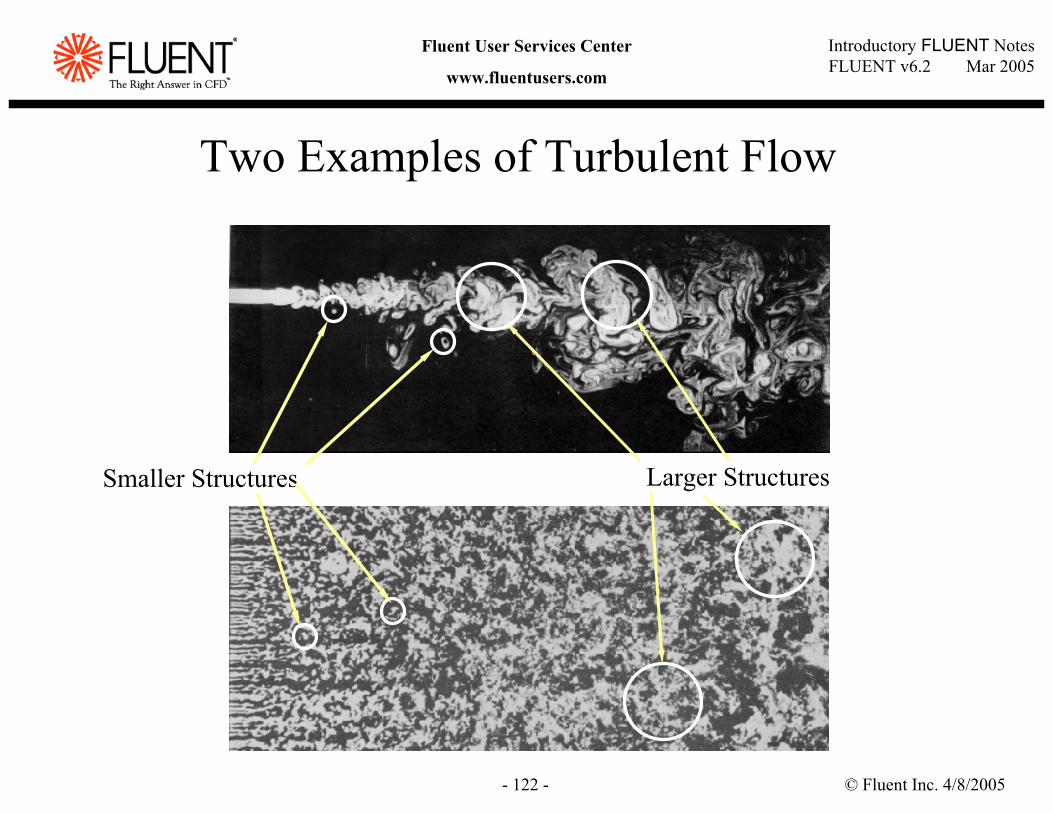
Two Examples of Turbulent Flow

Larger Structures Smaller Structures

© Fluent Inc. 4/8/2005- 123 -



www.fluentusers.com

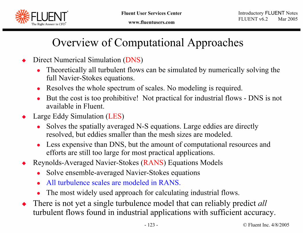
Overview of Computational ApproachesDirect Numerical Simulation (DNS)

Theoretically all turbulent flows can be simulated by numerically solving the full Navier-Stokes equations.Resolves the whole spectrum of scales. No modeling is required.But the cost is too prohibitive! Not practical for industrial flows - DNS is not available in Fluent.

Large Eddy Simulation (LES)Solves the spatially averaged N-S equations. Large eddies are directly resolved, but eddies smaller than the mesh sizes are modeled.Less expensive than DNS, but the amount of computational resources and efforts are still too large for most practical applications.

Reynolds-Averaged Navier-Stokes (RANS) Equations ModelsSolve ensemble-averaged Navier-Stokes equations All turbulence scales are modeled in RANS.The most widely used approach for calculating industrial flows.

There is not yet a single turbulence model that can reliably predict all turbulent flows found in industrial applications with sufficient accuracy.

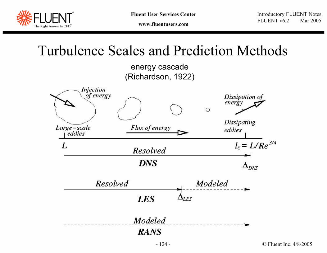
© Fluent Inc. 4/8/2005- 124 -



www.fluentusers.com

Turbulence Scales and Prediction Methodsenergy cascade

(Richardson, 1922)

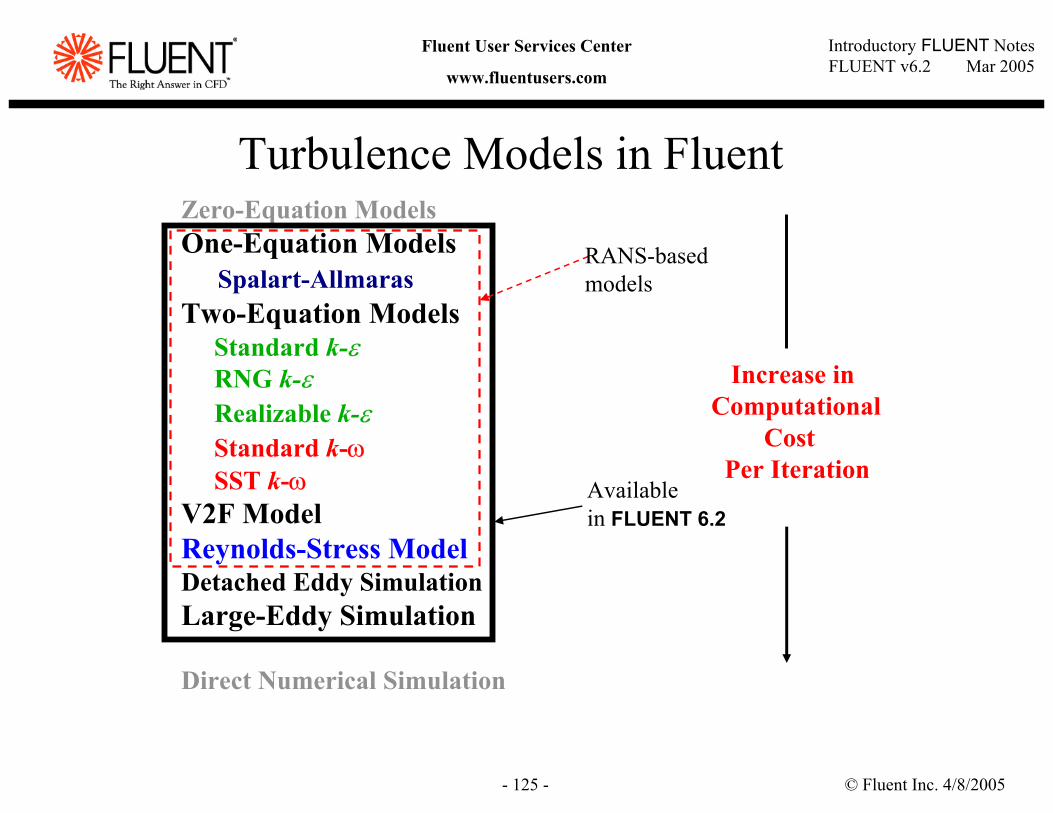
© Fluent Inc. 4/8/2005- 125 -



www.fluentusers.com

Zero-Equation ModelsOne-Equation Models

Spalart-AllmarasTwo-Equation Models

Standard k-εRNG k-εRealizable k-εStandard k-ωSST k-ω

V2F ModelReynolds-Stress ModelDetached Eddy SimulationLarge-Eddy Simulation

Direct Numerical Simulation

Turbulence Models in Fluent

Increase inComputational

CostPer Iteration

Availablein FLUENT 6.2

RANS-basedmodels

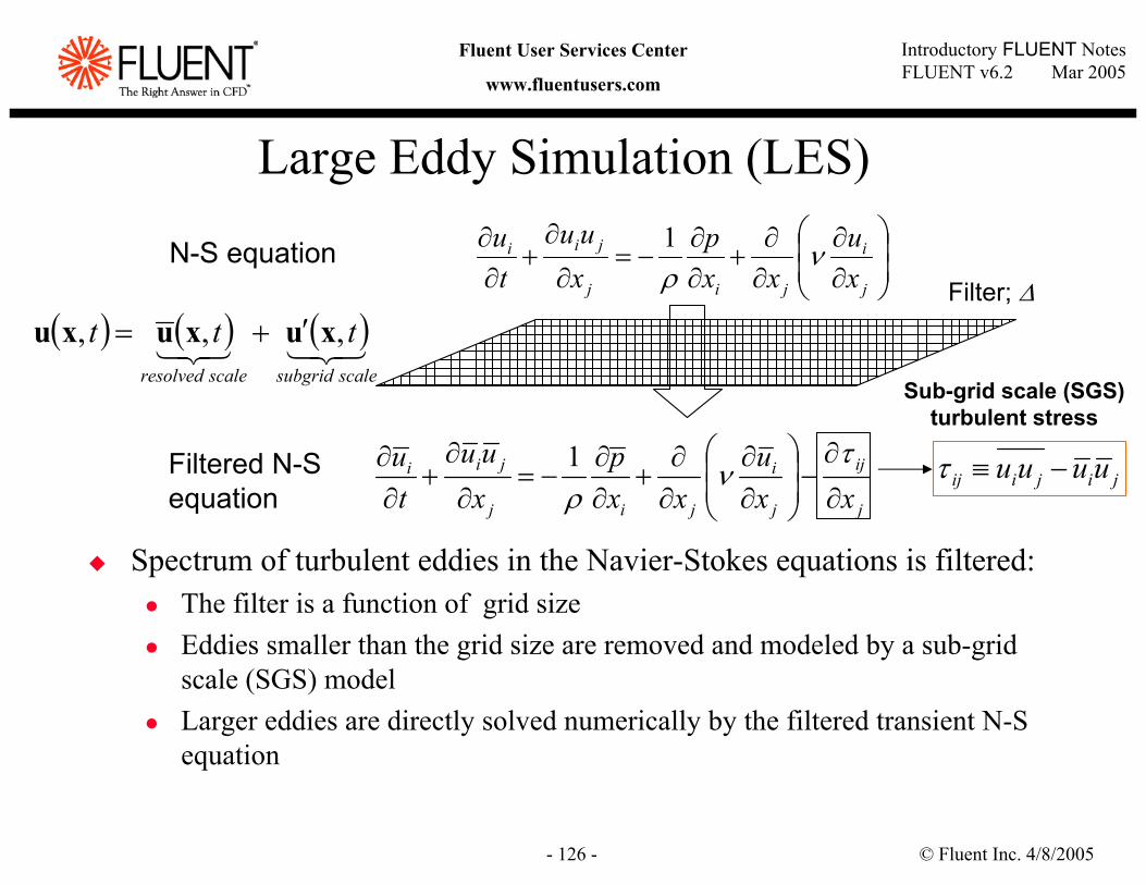
© Fluent Inc. 4/8/2005- 126 -



www.fluentusers.com

Large Eddy Simulation (LES)

Spectrum of turbulent eddies in the Navier-Stokes equations is filtered:The filter is a function of grid size Eddies smaller than the grid size are removed and modeled by a sub-grid scale (SGS) modelLarger eddies are directly solved numerically by the filtered transient N-S equation

( ) ( ) ( )321321 scalesubgrid scaleresolved

ttt ,,, xuxuxu ′+=

∂∂

∂∂

+∂∂

−=∂

∂+

∂∂

j

i

jij

jii

xu

xxp

xuu

tu ν

ρ1

j

ij

j

i

jij

jii

xxu

xxp

xuu

tu

∂

∂−

∂∂

∂∂

+∂∂

−=∂

∂+

∂∂ τ

νρ1

jijiij uuuu −≡τ

Filter; ∆

Sub-grid scale (SGS) turbulent stress

Filtered N-S equation

N-S equation

© Fluent Inc. 4/8/2005- 127 -



www.fluentusers.com

LES in FLUENTLES has been most successful for high-end applications where the RANS models fail to meet the needs. For example:

CombustionMixingExternal Aerodynamics (flows around bluff bodies)

Implementations in FLUENT:Sub-grid scale (SGS) turbulent models:

Smagorinsky-Lilly modelWALE model Dynamic Smagorinsky-Lilly model Dynamic kinetic energy transport modelDetached eddy simulation (DES) model

LES is applicable to all combustion models in FLUENTBasic statistical tools are available: Time averaged and root-mean-square (RMS) values of solution variables, built-in FFTBefore running LES, one should consult guidelines in the “Best Practices For LES” (containing advice for mesh, SGS models, numerics, BC’s, and more)

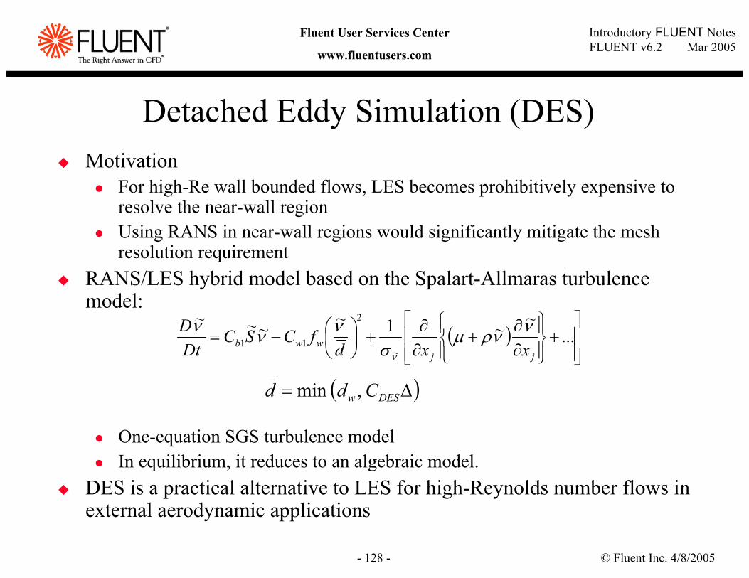
© Fluent Inc. 4/8/2005- 128 -



www.fluentusers.com

Detached Eddy Simulation (DES)Motivation

For high-Re wall bounded flows, LES becomes prohibitively expensive to resolve the near-wall region Using RANS in near-wall regions would significantly mitigate the mesh resolution requirement

RANS/LES hybrid model based on the Spalart-Allmaras turbulence model:

One-equation SGS turbulence modelIn equilibrium, it reduces to an algebraic model.

DES is a practical alternative to LES for high-Reynolds number flows in external aerodynamic applications

( )

+

∂∂

+∂∂

+

−= ...

~~1~~~~

~

2

11jj

wwb xxdfCSC

DtD ννρµ

σννν

ν

( )∆= DESw Cdd ,min

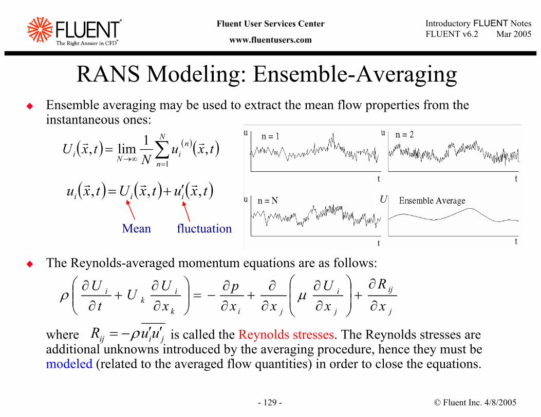
© Fluent Inc. 4/8/2005- 129 -



www.fluentusers.com

RANS Modeling: Ensemble-AveragingEnsemble averaging may be used to extract the mean flow properties from the instantaneous ones:

The Reynolds-averaged momentum equations are as follows:

where is called the Reynolds stresses. The Reynolds stresses are additional unknowns introduced by the averaging procedure, hence they must be modeled (related to the averaged flow quantities) in order to close the equations.

j

ij

j

i

jik

ik

i

xR

xU

xxp

xUU

tU

∂

∂+

∂∂

∂∂

+∂∂

−=

∂∂

+∂

∂ µρ

jiij uuR ′′−= ρ

( ) ( )( )∑=

∞→=

N

n

niNi txu

NtxU

1,1lim, rr

( ) ( ) ( )txutxUtxu iii ,,, rrr ′+=U

fluctuationMean

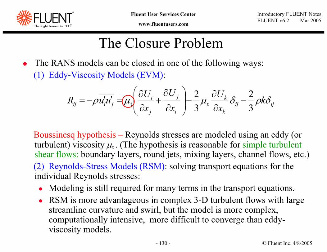
© Fluent Inc. 4/8/2005- 130 -



www.fluentusers.com

The Closure ProblemThe RANS models can be closed in one of the following ways:(1) Eddy-Viscosity Models (EVM):

Boussinesq hypothesis – Reynolds stresses are modeled using an eddy (or turbulent) viscosity µt . (The hypothesis is reasonable for simple turbulent shear flows: boundary layers, round jets, mixing layers, channel flows, etc.)(2) Reynolds-Stress Models (RSM): solving transport equations for the individual Reynolds stresses:

Modeling is still required for many terms in the transport equations.RSM is more advantageous in complex 3-D turbulent flows with large streamline curvature and swirl, but the model is more complex, computationally intensive, more difficult to converge than eddy-viscosity models.

ijijk

k

i

j

j

ijiij k

xU

xU

xUuuR δρδµµρ

32

32

tt −∂∂

−

∂

∂+

∂∂

=′′−=

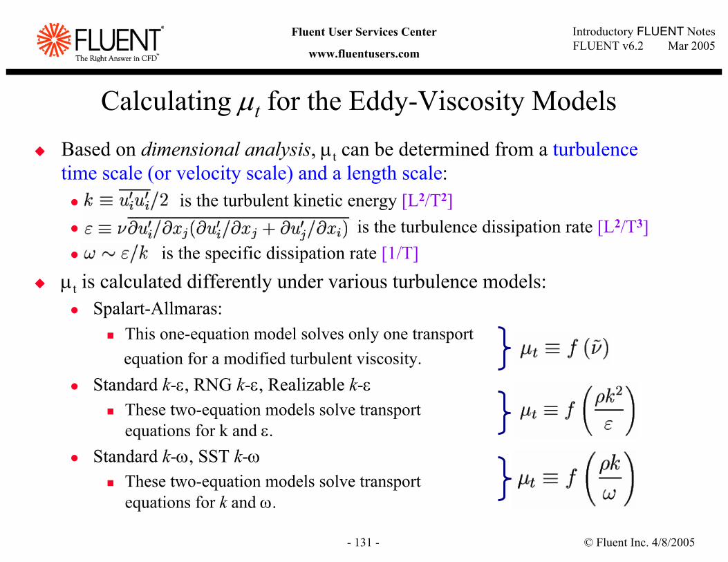
© Fluent Inc. 4/8/2005- 131 -



www.fluentusers.com

Calculating µt for the Eddy-Viscosity ModelsBased on dimensional analysis, µt can be determined from a turbulence time scale (or velocity scale) and a length scale:

is the turbulent kinetic energy [L2/T2]is the turbulence dissipation rate [L2/T3]

is the specific dissipation rate [1/T]µt is calculated differently under various turbulence models:

Spalart-Allmaras:This one-equation model solves only one transportequation for a modified turbulent viscosity.

Standard k-ε, RNG k-ε, Realizable k-εThese two-equation models solve transport equations for k and ε.

Standard k-ω, SST k-ωThese two-equation models solve transportequations for k and ω.

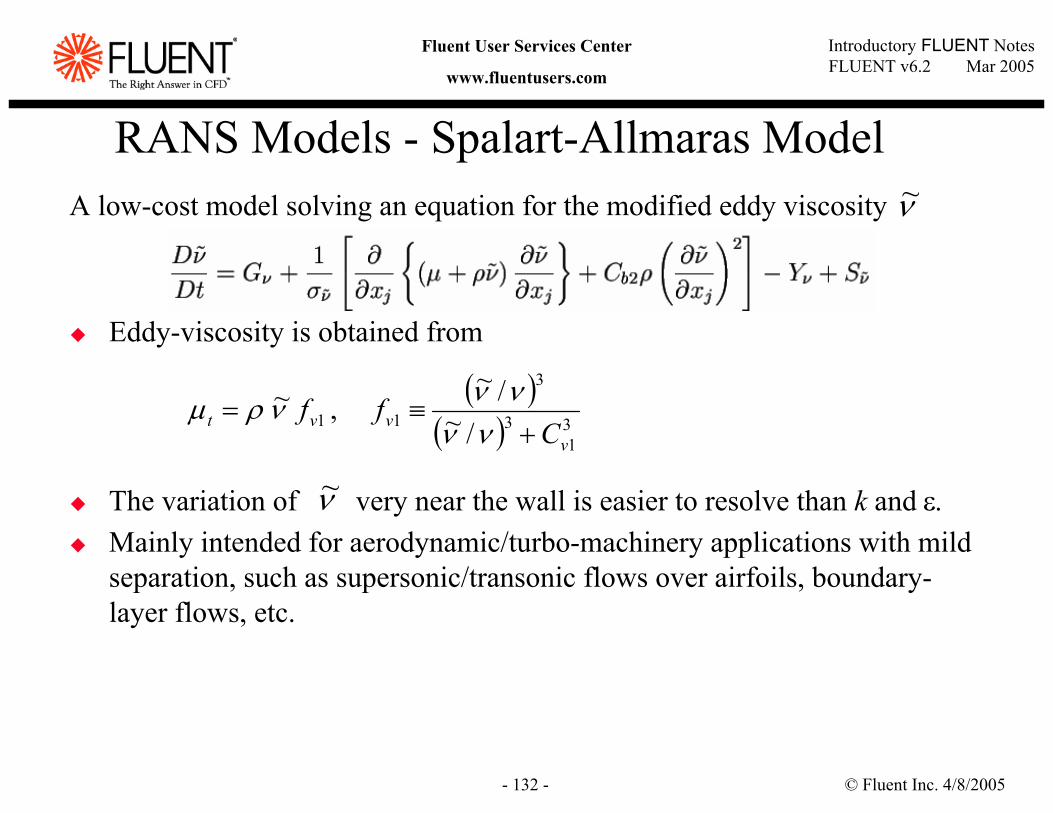
© Fluent Inc. 4/8/2005- 132 -



www.fluentusers.com

RANS Models - Spalart-Allmaras ModelA low-cost model solving an equation for the modified eddy viscosity

Eddy-viscosity is obtained from

The variation of very near the wall is easier to resolve than k and ε.Mainly intended for aerodynamic/turbo-machinery applications with mild separation, such as supersonic/transonic flows over airfoils, boundary-layer flows, etc.

( )( ) 3

13

3

11 /~/~

,~v

vvt Cff

+≡=

νννννρµ

ν~

ν~

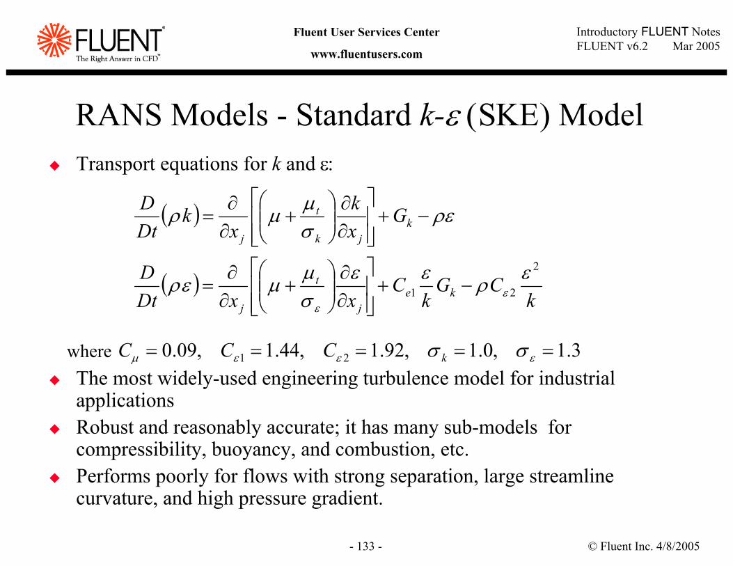
© Fluent Inc. 4/8/2005- 133 -



www.fluentusers.com

RANS Models - Standard k-ε (SΚΕ) Model Transport equations for k and ε:

The most widely-used engineering turbulence model for industrial applicationsRobust and reasonably accurate; it has many sub-models for compressibility, buoyancy, and combustion, etc.Performs poorly for flows with strong separation, large streamline curvature, and high pressure gradient.

( )

( )k

CGk

CxxDt

D

Gxk

xk

DtD

kej

t

j

kjk

t

j

2

21ερεε

σµµερ

ρεσµµρ

εε

−+

∂∂

+

∂∂

=

−+

∂∂

+

∂∂

=

3.1,0.1,92.1,44.1,09.0 21 ===== εεεµ σσ kCCCwhere

© Fluent Inc. 4/8/2005- 134 -



www.fluentusers.com

RANS Models - Realizable k-ε (RΚΕ) Model

Realizable k-ε (RKE) model ensures “realizability” of the k-ε model, i.e., Positivity of normal stressesSchwarz’ inequality for Reynolds shear-stresses

Good performance for flows with axisymmetric jets.

RANS Models - RNG k-ε ModelConstants in the k-ε equations are derived using the Renormalization Group method.

RNG’s sub-models include:Differential viscosity model to account for low-Re effects

Analytically derived algebraic formula for turbulent Prandtl/Schmidt number

Swirl modification

Performs better than SKE for more complex shear flows, and flows with high strain rates, swirl, and separation.

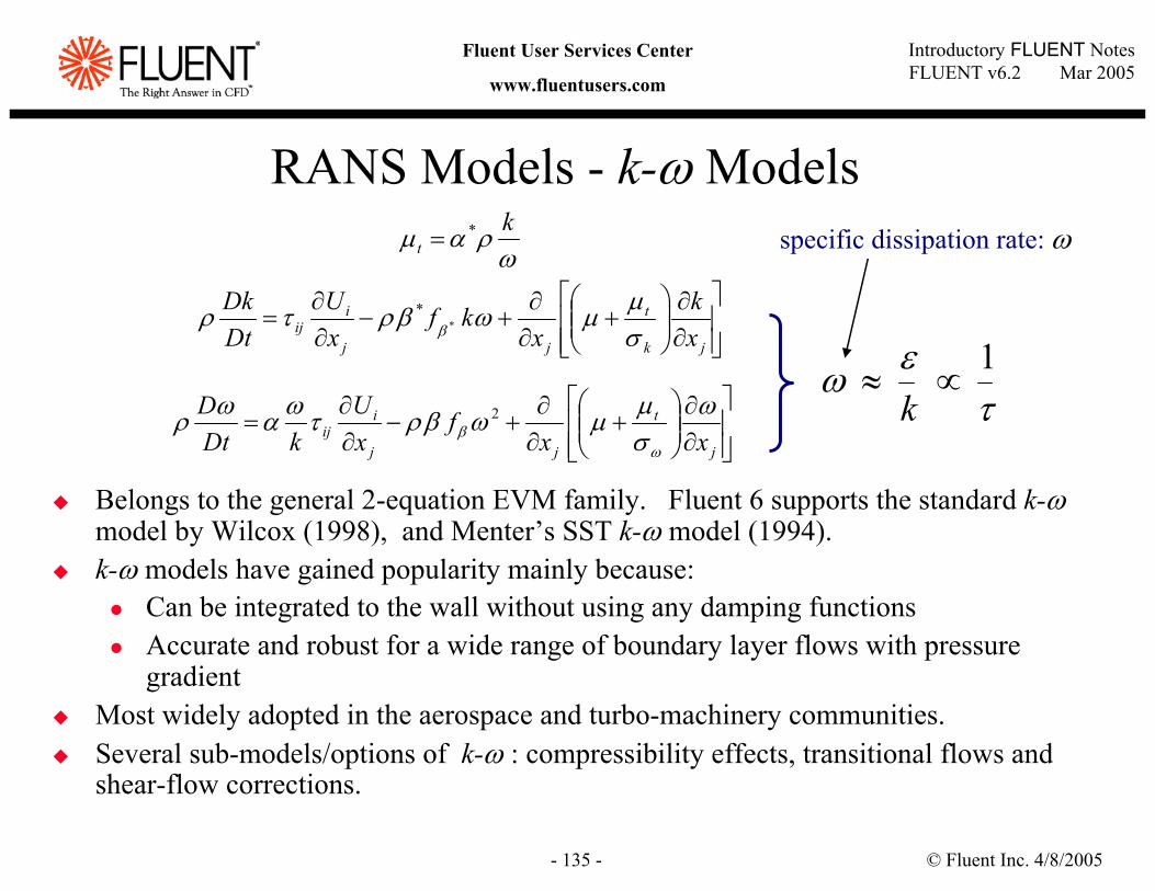
© Fluent Inc. 4/8/2005- 135 -



www.fluentusers.com

RANS Models - k-ω Models

Belongs to the general 2-equation EVM family. Fluent 6 supports the standard k-ωmodel by Wilcox (1998), and Menter’s SST k-ω model (1994).k-ω models have gained popularity mainly because:

Can be integrated to the wall without using any damping functionsAccurate and robust for a wide range of boundary layer flows with pressure gradient

Most widely adopted in the aerospace and turbo-machinery communities.Several sub-models/options of k-ω : compressibility effects, transitional flows and shear-flow corrections.

∂∂

+

∂∂

+−∂∂

=

∂∂

+

∂∂

+−∂∂

=

=

j

t

jj

iij

jk

t

jj

iij

t

xxf

xU

kDtD

xk

xkf

xU

DtDk

k

ωσµµωβρτωαωρ

σµµωβρτρ

ωραµ

ωβ

β

2

*

*

*

τεω 1

∝≈k

specific dissipation rate: ω

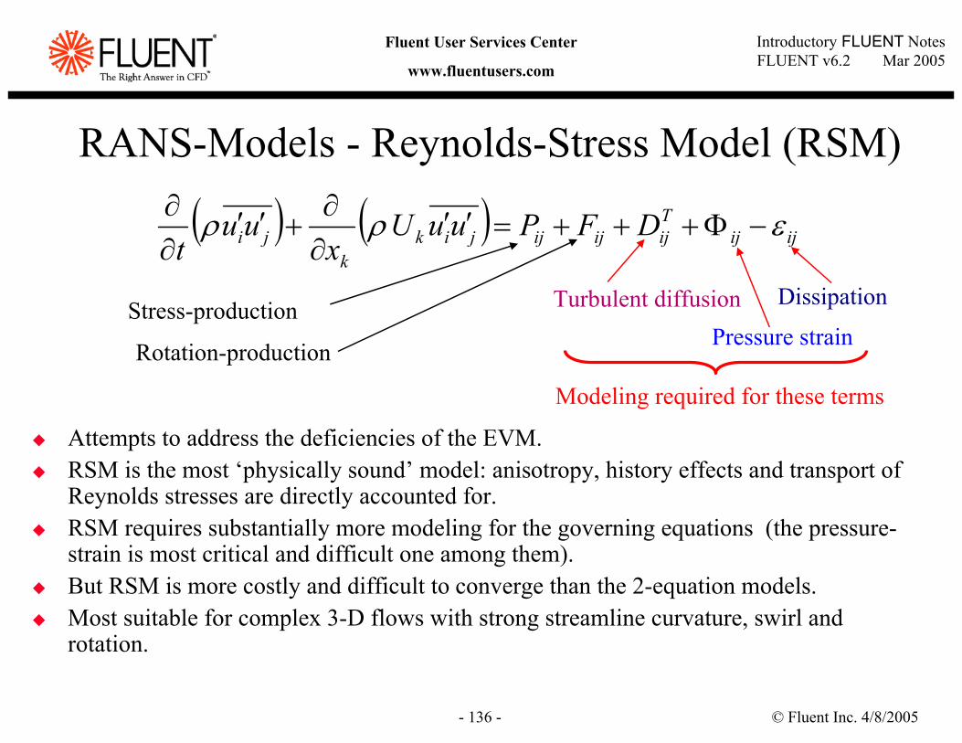
© Fluent Inc. 4/8/2005- 136 -



www.fluentusers.com

RANS-Models - Reynolds-Stress Model (RSM)

( ) ( ) ijijTijijijjik

kji DFPuuU

xuu

tερρ −Φ+++=′′

∂∂

+′′∂∂

Turbulent diffusionStress-production

Rotation-production Pressure strain

Dissipation

Modeling required for these terms

Attempts to address the deficiencies of the EVM.RSM is the most ‘physically sound’ model: anisotropy, history effects and transport of Reynolds stresses are directly accounted for. RSM requires substantially more modeling for the governing equations (the pressure-strain is most critical and difficult one among them).But RSM is more costly and difficult to converge than the 2-equation models.Most suitable for complex 3-D flows with strong streamline curvature, swirl and rotation.

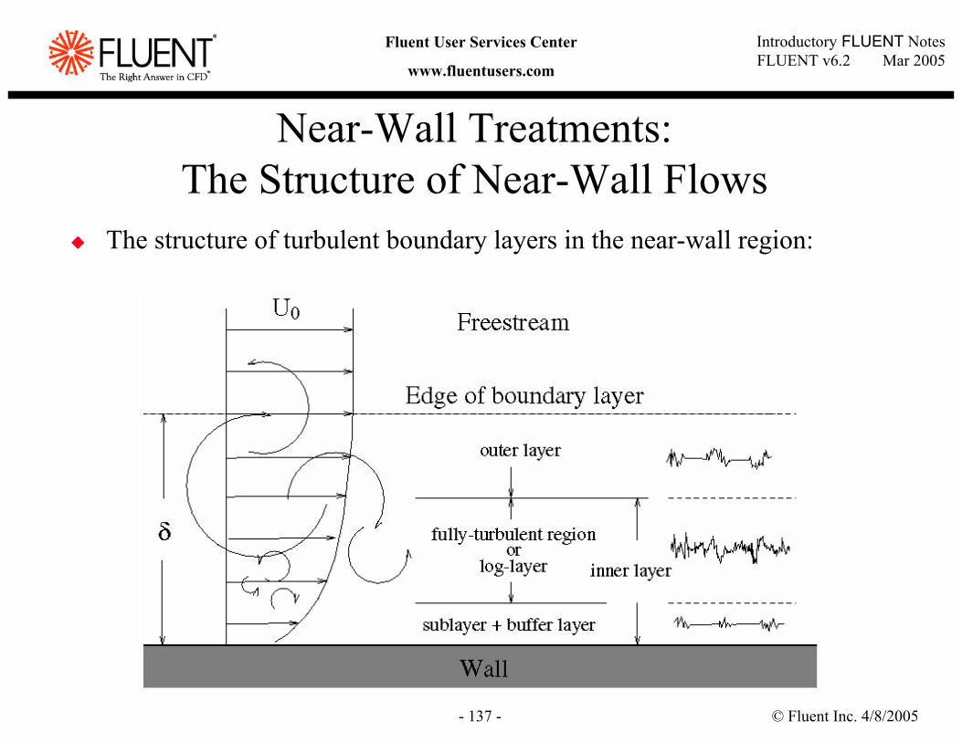
© Fluent Inc. 4/8/2005- 137 -



www.fluentusers.com

Near-Wall Treatments:The Structure of Near-Wall Flows

The structure of turbulent boundary layers in the near-wall region:

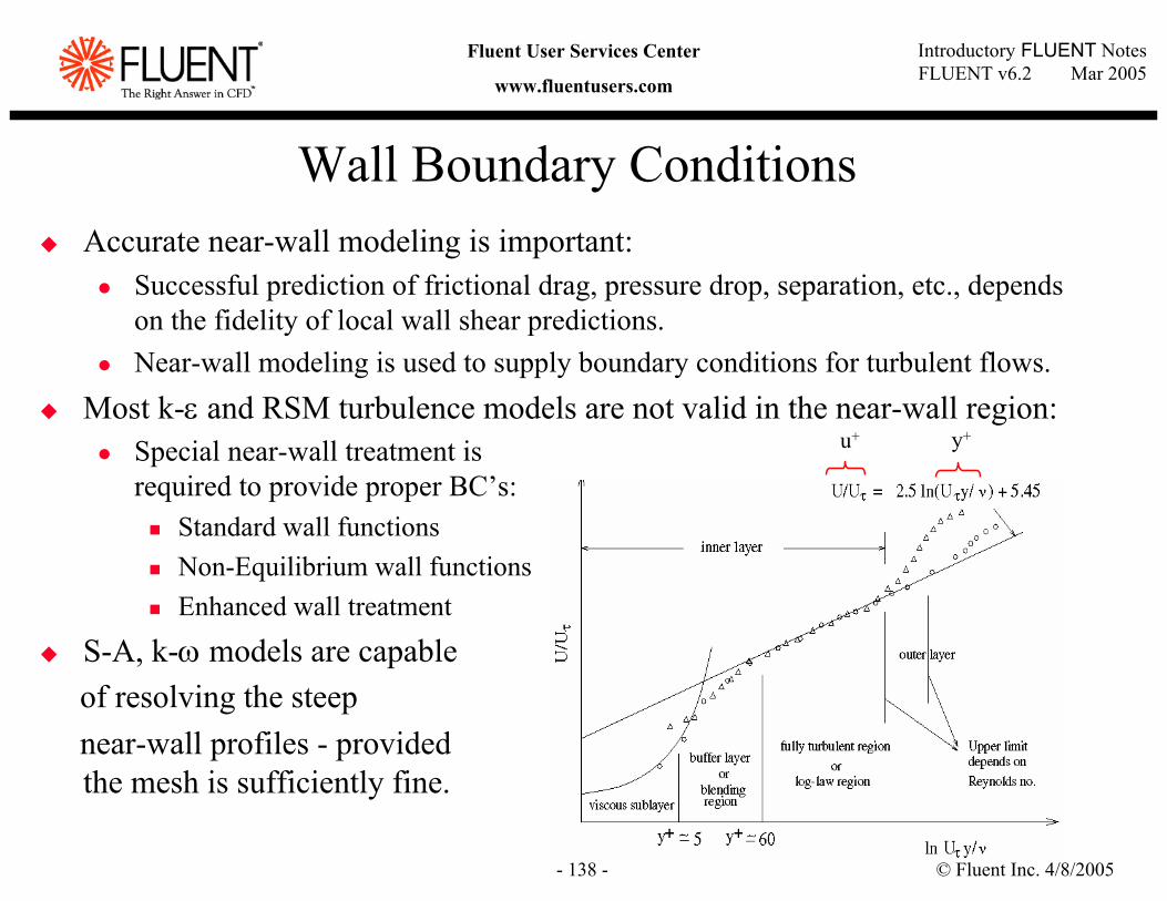
© Fluent Inc. 4/8/2005- 138 -



www.fluentusers.com

Accurate near-wall modeling is important:Successful prediction of frictional drag, pressure drop, separation, etc., depends on the fidelity of local wall shear predictions.Near-wall modeling is used to supply boundary conditions for turbulent flows.

Most k-ε and RSM turbulence models are not valid in the near-wall region:Special near-wall treatment is required to provide proper BC’s:

Standard wall functionsNon-Equilibrium wall functionsEnhanced wall treatment

S-A, k-ω models are capable of resolving the steep near-wall profiles - provided the mesh is sufficiently fine.

u+ y+

Wall Boundary Conditions

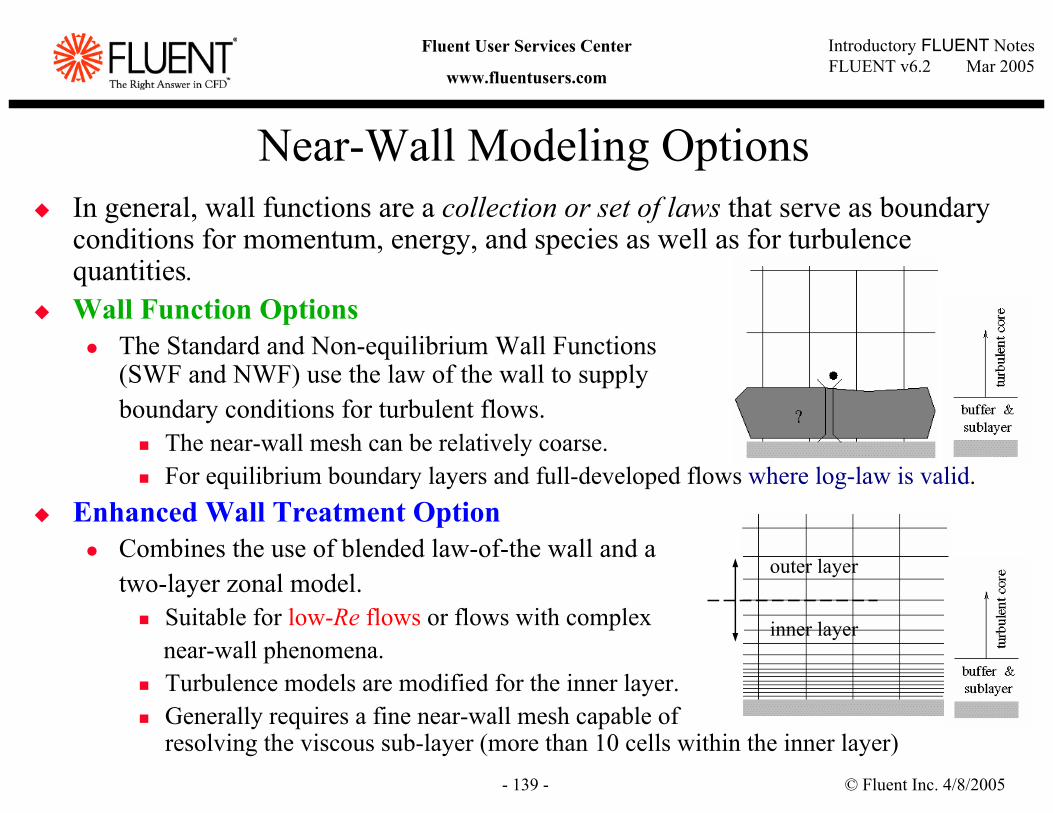
© Fluent Inc. 4/8/2005- 139 -



www.fluentusers.com

In general, wall functions are a collection or set of laws that serve as boundary conditions for momentum, energy, and species as well as for turbulence quantities.Wall Function Options

The Standard and Non-equilibrium Wall Functions(SWF and NWF) use the law of the wall to supply boundary conditions for turbulent flows.

The near-wall mesh can be relatively coarse.For equilibrium boundary layers and full-developed flows where log-law is valid.

Enhanced Wall Treatment OptionCombines the use of blended law-of-the wall and atwo-layer zonal model.

Suitable for low-Re flows or flows with complex near-wall phenomena.Turbulence models are modified for the inner layer.Generally requires a fine near-wall mesh capable of resolving the viscous sub-layer (more than 10 cells within the inner layer)

Near-Wall Modeling Options

inner layer

outer layer

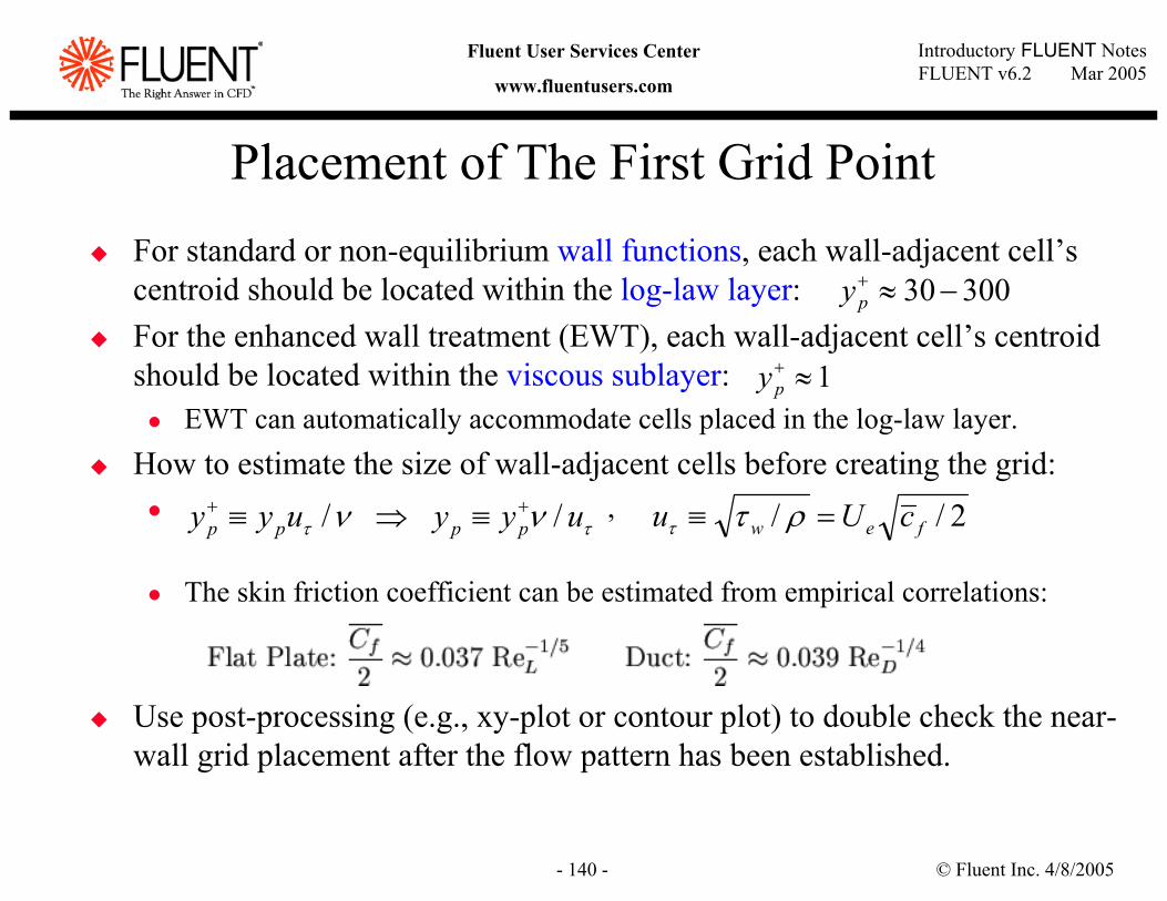
© Fluent Inc. 4/8/2005- 140 -



www.fluentusers.com

Placement of The First Grid PointFor standard or non-equilibrium wall functions, each wall-adjacent cell’s centroid should be located within the log-law layer:For the enhanced wall treatment (EWT), each wall-adjacent cell’s centroidshould be located within the viscous sublayer:

EWT can automatically accommodate cells placed in the log-law layer.How to estimate the size of wall-adjacent cells before creating the grid:

,

The skin friction coefficient can be estimated from empirical correlations:

Use post-processing (e.g., xy-plot or contour plot) to double check the near-wall grid placement after the flow pattern has been established.

2// few cUu =≡ ρττ

30030 −≈+py

1≈+py

ττ νν uyyuyy pppp // ++ ≡⇒≡

© Fluent Inc. 4/8/2005- 141 -



www.fluentusers.com

Near-Wall Modeling: Recommended Strategy

Use SWF or NWF for most high Re applications (Re > 106) for which you cannot afford to resolve the viscous sub-layer.

There is little gain from resolving the viscous sub-layer. The choice of core turbulence model is more important.Use NWF for mildly separating, reattaching, or impinging flows.

You may consider using EWT if:The characteristic Re is low or if near wall characteristics need to be resolved.The same or similar cases which ran successfully previously with the two-layer zonal model (in Fluent v5).The physics and near-wall mesh of the case is such that y+ is likely to vary significantly over a wide portion of the wall region.

Try to make the mesh either coarse or fine enough to avoid placing the wall-adjacent cells in the buffer layer (y+ = 5 ~ 30).

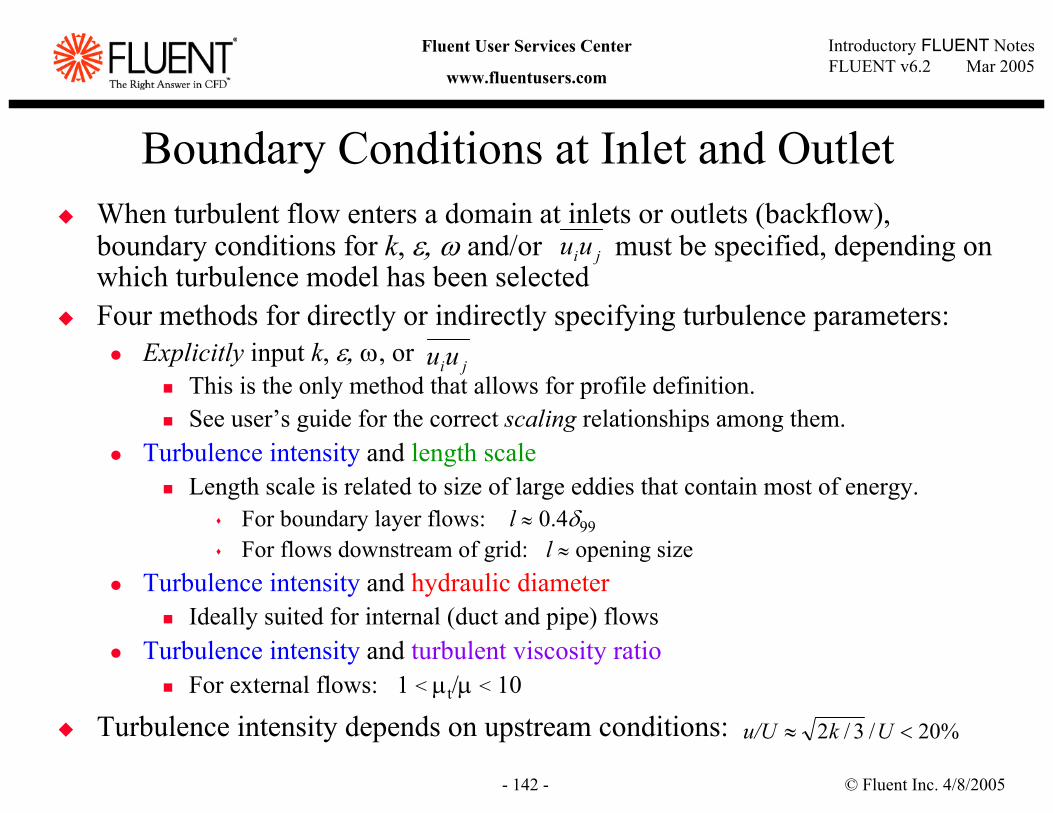
© Fluent Inc. 4/8/2005- 142 -



www.fluentusers.com

Boundary Conditions at Inlet and OutletWhen turbulent flow enters a domain at inlets or outlets (backflow), boundary conditions for k, ε, ω and/or must be specified, depending on which turbulence model has been selectedFour methods for directly or indirectly specifying turbulence parameters:

Explicitly input k, ε, ω, orThis is the only method that allows for profile definition.See user’s guide for the correct scaling relationships among them.

Turbulence intensity and length scaleLength scale is related to size of large eddies that contain most of energy.

For boundary layer flows: l ≈ 0.4δ99For flows downstream of grid: l ≈ opening size

Turbulence intensity and hydraulic diameterIdeally suited for internal (duct and pipe) flows

Turbulence intensity and turbulent viscosity ratioFor external flows: 1 < µt/µ < 10

Turbulence intensity depends on upstream conditions:

jiuu

jiuu

%20/3/2 <≈ Uku/U

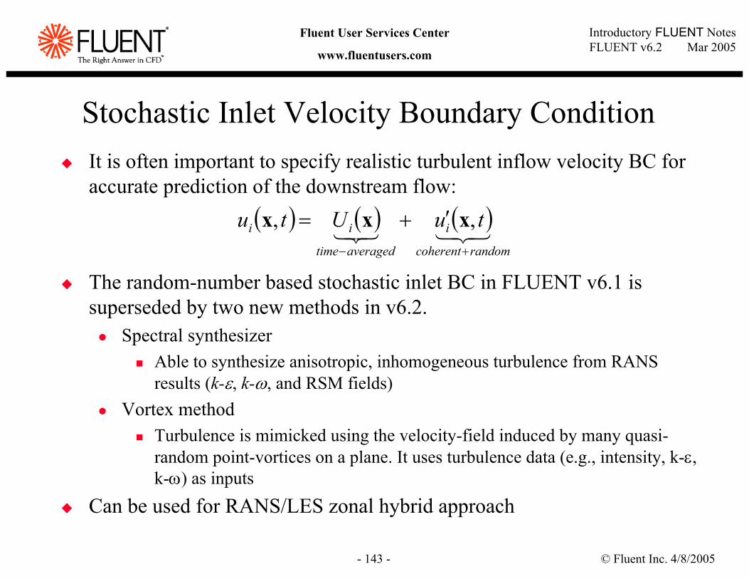
© Fluent Inc. 4/8/2005- 143 -



www.fluentusers.com

Stochastic Inlet Velocity Boundary ConditionIt is often important to specify realistic turbulent inflow velocity BC for accurate prediction of the downstream flow:

The random-number based stochastic inlet BC in FLUENT v6.1 is superseded by two new methods in v6.2.

Spectral synthesizerAble to synthesize anisotropic, inhomogeneous turbulence from RANS results (k-ε, k-ω, and RSM fields)

Vortex methodTurbulence is mimicked using the velocity-field induced by many quasi-random point-vortices on a plane. It uses turbulence data (e.g., intensity, k-ε, k-ω) as inputs

Can be used for RANS/LES zonal hybrid approach

( ) ( ) ( )321321randomcoherent

i

averagedtime

ii tuUtu+−

′+= ,, xxx

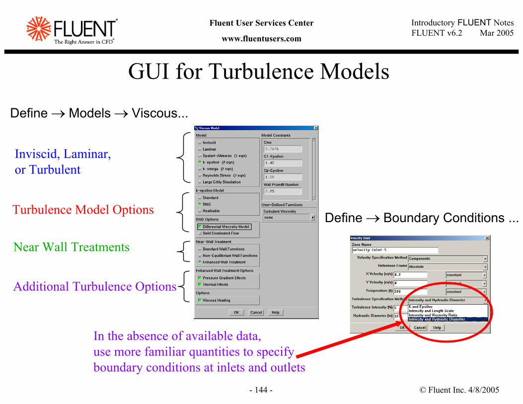
© Fluent Inc. 4/8/2005- 144 -



www.fluentusers.com

GUI for Turbulence Models

Define → Models → Viscous...

Turbulence Model Options

Near Wall Treatments

Inviscid, Laminar, or Turbulent

Additional Turbulence Options

Define → Boundary Conditions ...

In the absence of available data,use more familiar quantities to specifyboundary conditions at inlets and outlets

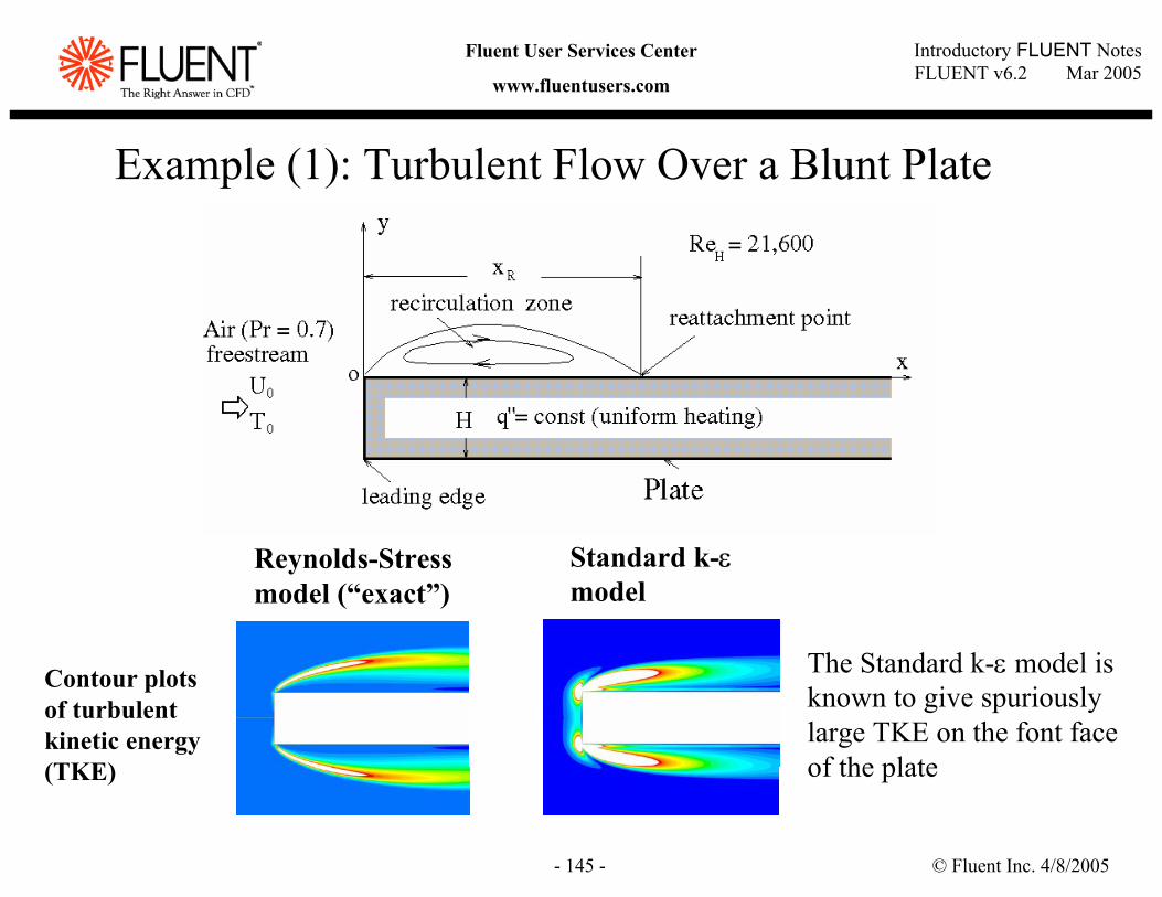
© Fluent Inc. 4/8/2005- 145 -



www.fluentusers.com

Example (1): Turbulent Flow Over a Blunt Plate

Standard k-εmodel

Reynolds-Stress model (“exact”)

Contour plots of turbulent kinetic energy (TKE)

The Standard k-ε model is known to give spuriously large TKE on the font face of the plate

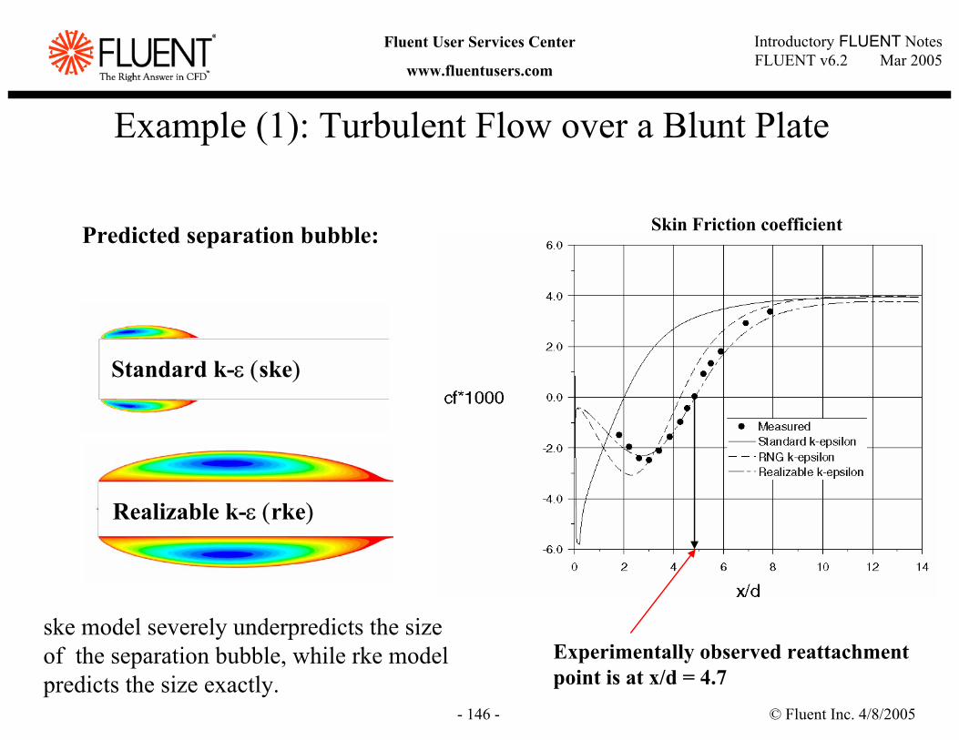
© Fluent Inc. 4/8/2005- 146 -



www.fluentusers.com

Experimentally observed reattachment point is at x/d = 4.7

Predicted separation bubble:

Example (1): Turbulent Flow over a Blunt Plate

Standard k-ε (ske)

Skin Friction coefficient

Realizable k-ε (rke)

ske model severely underpredicts the size of the separation bubble, while rke model predicts the size exactly.

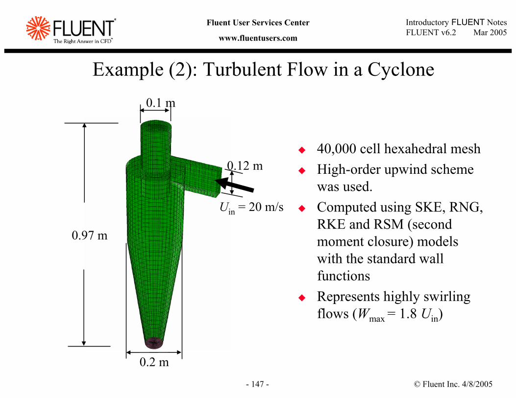
© Fluent Inc. 4/8/2005- 147 -



www.fluentusers.com

Example (2): Turbulent Flow in a Cyclone

40,000 cell hexahedral meshHigh-order upwind scheme was used.Computed using SKE, RNG, RKE and RSM (second moment closure) models with the standard wall functionsRepresents highly swirling flows (Wmax = 1.8 Uin)

0.97 m

0.1 m

0.2 m

Uin = 20 m/s

0.12 m

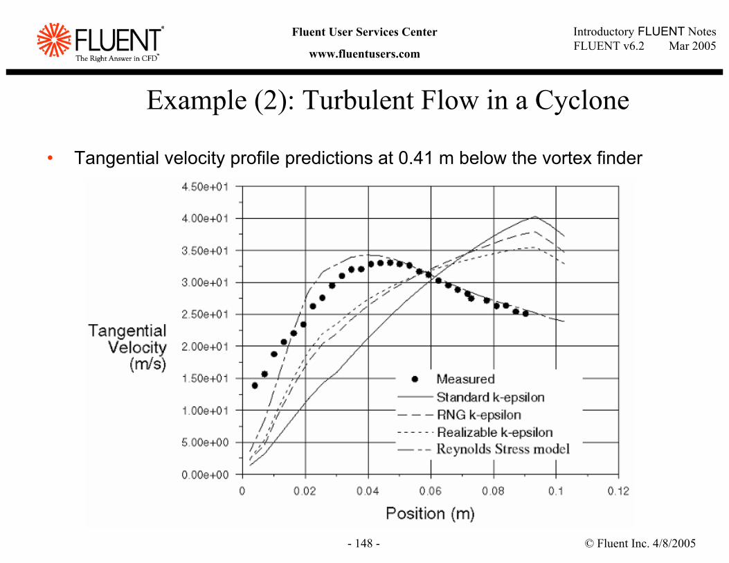
© Fluent Inc. 4/8/2005- 148 -



www.fluentusers.com

• Tangential velocity profile predictions at 0.41 m below the vortex finder

Example (2): Turbulent Flow in a Cyclone

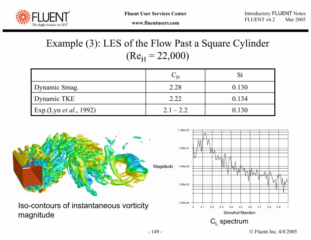
© Fluent Inc. 4/8/2005- 149 -



www.fluentusers.com

Example (3): LES of the Flow Past a Square Cylinder (ReH = 22,000)

Iso-contours of instantaneous vorticitymagnitude

Time-averaged streamwisevelocity along the wake centerline

0.1302.1 – 2.2Exp.(Lyn et al., 1992)

0.1342.22Dynamic TKE

0.1302.28Dynamic Smag.

StCD

CL spectrum

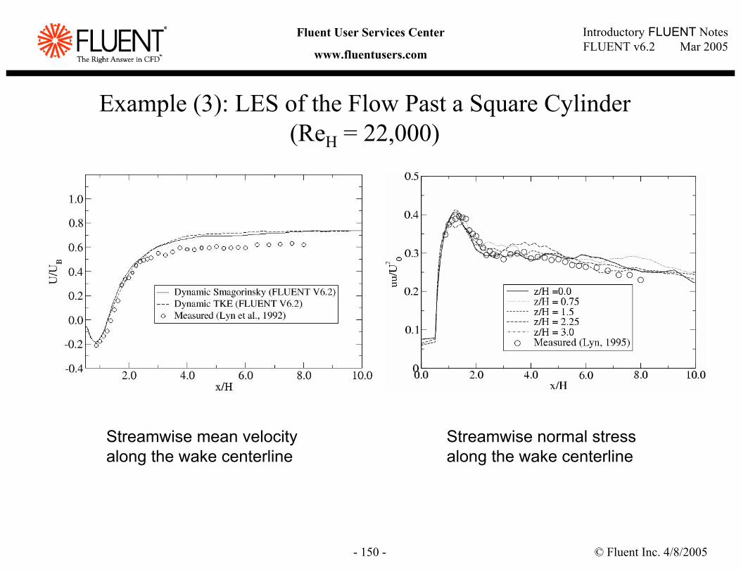
© Fluent Inc. 4/8/2005- 150 -



www.fluentusers.com

Streamwise mean velocity along the wake centerline

Streamwise normal stress along the wake centerline

Example (3): LES of the Flow Past a Square Cylinder (ReH = 22,000)

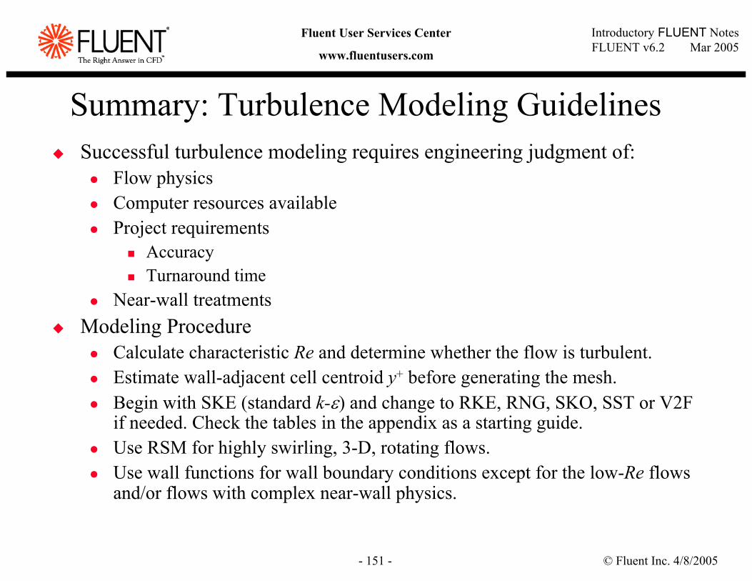
© Fluent Inc. 4/8/2005- 151 -



www.fluentusers.com

Summary: Turbulence Modeling GuidelinesSuccessful turbulence modeling requires engineering judgment of:

Flow physicsComputer resources availableProject requirements

AccuracyTurnaround time

Near-wall treatmentsModeling Procedure

Calculate characteristic Re and determine whether the flow is turbulent.Estimate wall-adjacent cell centroid y+ before generating the mesh.Begin with SKE (standard k-ε) and change to RKE, RNG, SKO, SST or V2F if needed. Check the tables in the appendix as a starting guide.Use RSM for highly swirling, 3-D, rotating flows.Use wall functions for wall boundary conditions except for the low-Re flows and/or flows with complex near-wall physics.

© Fluent Inc. 4/8/2005- 152 -



www.fluentusers.com

Appendix

Summary of RANS Turbulence Models: Description, Model Behavior and UsageMore Details on Near-wall ModelingTurbulent Heat Transfer ModelingAdditional Information on Menter’s SST k-ω ModelV2F Turbulence ModelInitial Velocity Field for LES/DES

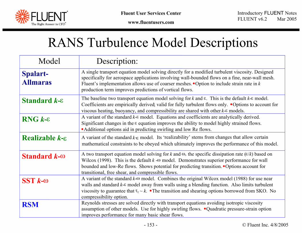
© Fluent Inc. 4/8/2005- 153 -



www.fluentusers.com

RANS Turbulence Model DescriptionsModel Description:

Spalart-Allmaras

A single transport equation model solving directly for a modified turbulent viscosity. Designedspecifically for aerospace applications involving wall-bounded flows on a fine, near-wall mesh.Fluent’s implementation allows use of coarser meshes. •Option to include strain rate in kproduction term improves predictions of vortical flows.

Standard k-ε The baseline two transport equation model solving for k and ε. This is the default k-ε model.Coefficients are empirically derived; valid for fully turbulent flows only. •Options to account forviscous heating, buoyancy, and compressibility are shared with other k-ε models.

RNG k-ε A variant of the standard k-ε model. Equations and coefficients are analytically derived.Significant changes in the ε equation improves the ability to model highly strained flows.•Additional options aid in predicting swirling and low Re flows.

Realizable k-ε A variant of the standard k-ε model. Its ‘realizability’ stems from changes that allow certainmathematical constraints to be obeyed which ultimately improves the performance of this model.

Standard k-ω A two transport equation model solving for k and ω, the specific dissipation rate (ε/k) based onWilcox (1998). This is the default k -ω model. Demonstrates superior performance for wallbounded and low-Re flows. Shows potential for predicting transition. •Options account fortransitional, free shear, and compressible flows.

SST k-ω A variant of the standard k-ω model. Combines the original Wilcox model (1988) for use nearwalls and standard k-ε model away from walls using a blending function. Also limits turbulentviscosity to guarantee that τt ~ k. •The transition and shearing options borrowed from SKO. Nocompressibility option.

RSM Reynolds stresses are solved directly with transport equations avoiding isotropic viscosityassumption of other models. Use for highly swirling flows. •Quadratic pressure-strain optionimproves performance for many basic shear flows.

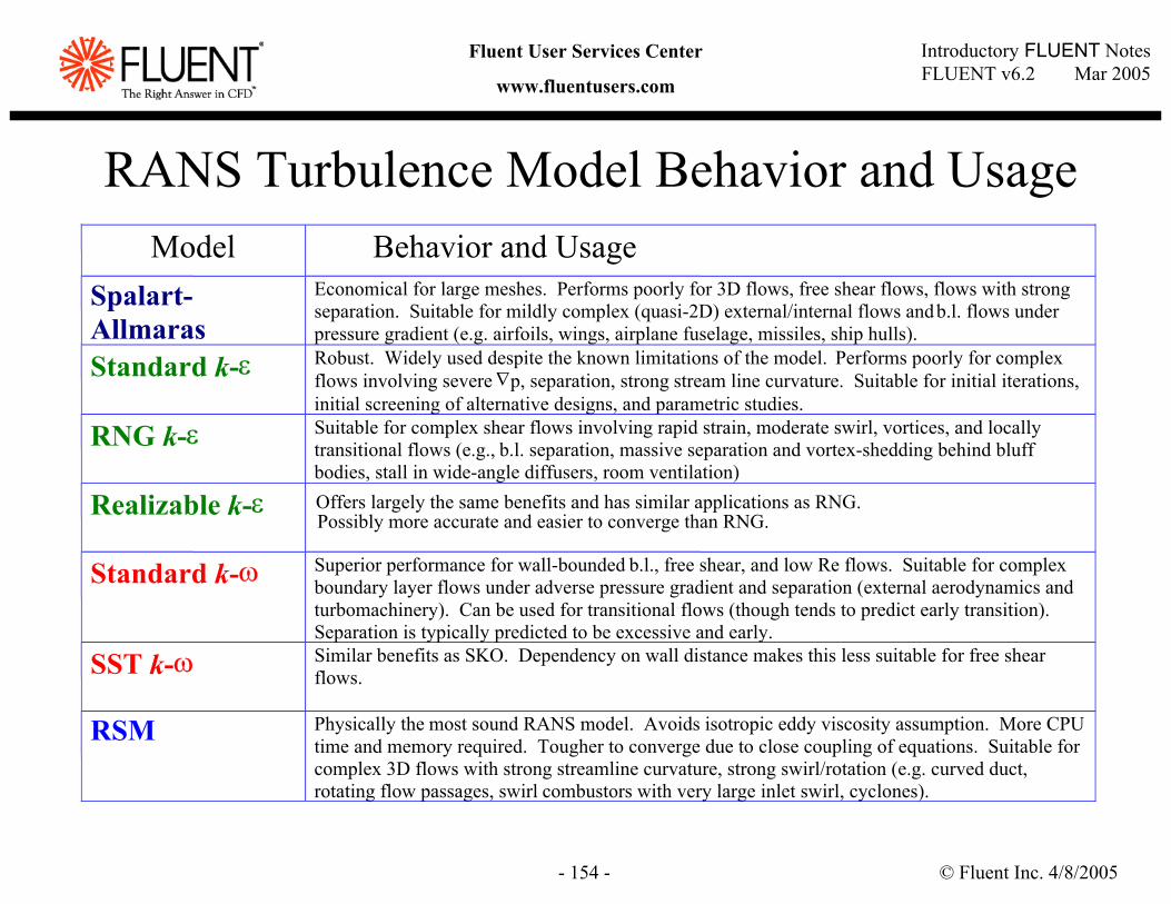
© Fluent Inc. 4/8/2005- 154 -



www.fluentusers.com

RANS Turbulence Model Behavior and UsageModel Behavior and Usage

Spalart-Allmaras

Economical for large meshes. Performs poorly for 3D flows, free shear flows, flows with strongseparation. Suitable for mildly complex (quasi-2D) external/internal flows and b.l. flows underpressure gradient (e.g. airfoils, wings, airplane fuselage, missiles, ship hulls).

Standard k-ε Robust. Widely used despite the known limitations of the model. Performs poorly for complexflows involving severe ∇p, separation, strong stream line curvature. Suitable for initial iterations,initial screening of alternative designs, and parametric studies.

RNG k-ε Suitable for complex shear flows involving rapid strain, moderate swirl, vortices, and locallytransitional flows (e.g., b.l. separation, massive separation and vortex-shedding behind bluffbodies, stall in wide-angle diffusers, room ventilation)

Realizable k-ε Offers largely the same benefits and has similar applications as RNG. Possibly more accurate and easier to converge than RNG.

Standard k-ω Superior performance for wall-bounded b.l., free shear, and low Re flows. Suitable for complexboundary layer flows under adverse pressure gradient and separation (external aerodynamics andturbomachinery). Can be used for transitional flows (though tends to predict early transition).Separation is typically predicted to be excessive and early.

SST k-ω Similar benefits as SKO. Dependency on wall distance makes this less suitable for free shearflows.

RSM Physically the most sound RANS model. Avoids isotropic eddy viscosity assumption. More CPUtime and memory required. Tougher to converge due to close coupling of equations. Suitable forcomplex 3D flows with strong streamline curvature, strong swirl/rotation (e.g. curved duct,rotating flow passages, swirl combustors with very large inlet swirl, cyclones).

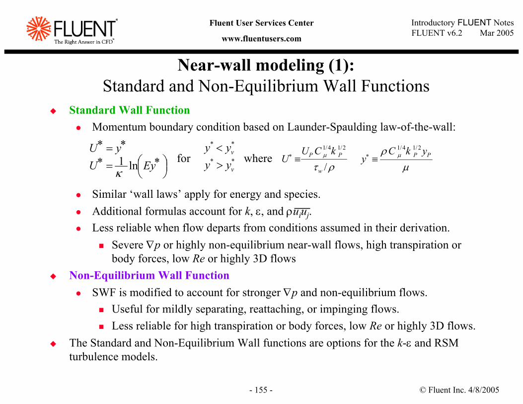
© Fluent Inc. 4/8/2005- 155 -



www.fluentusers.com

Standard Wall FunctionMomentum boundary condition based on Launder-Spaulding law-of-the-wall:

Similar ‘wall laws’ apply for energy and species.Additional formulas account for k, ε, and ρuiuj.Less reliable when flow departs from conditions assumed in their derivation.

Severe ∇p or highly non-equilibrium near-wall flows, high transpiration or body forces, low Re or highly 3D flows

Non-Equilibrium Wall FunctionSWF is modified to account for stronger ∇p and non-equilibrium flows.

Useful for mildly separating, reattaching, or impinging flows.Less reliable for high transpiration or body forces, low Re or highly 3D flows.

The Standard and Non-Equilibrium Wall functions are options for the k-ε and RSM turbulence models.

ρτµ

/

2/14/1

w

PP kCUU ≡∗

µρ µ PP ykC

y2/14/1

≡∗where

∗=∗ EyU ln1

κ

∗=∗ yUfor

**vyy <**vyy >

Near-wall modeling (1):Standard and Non-Equilibrium Wall Functions

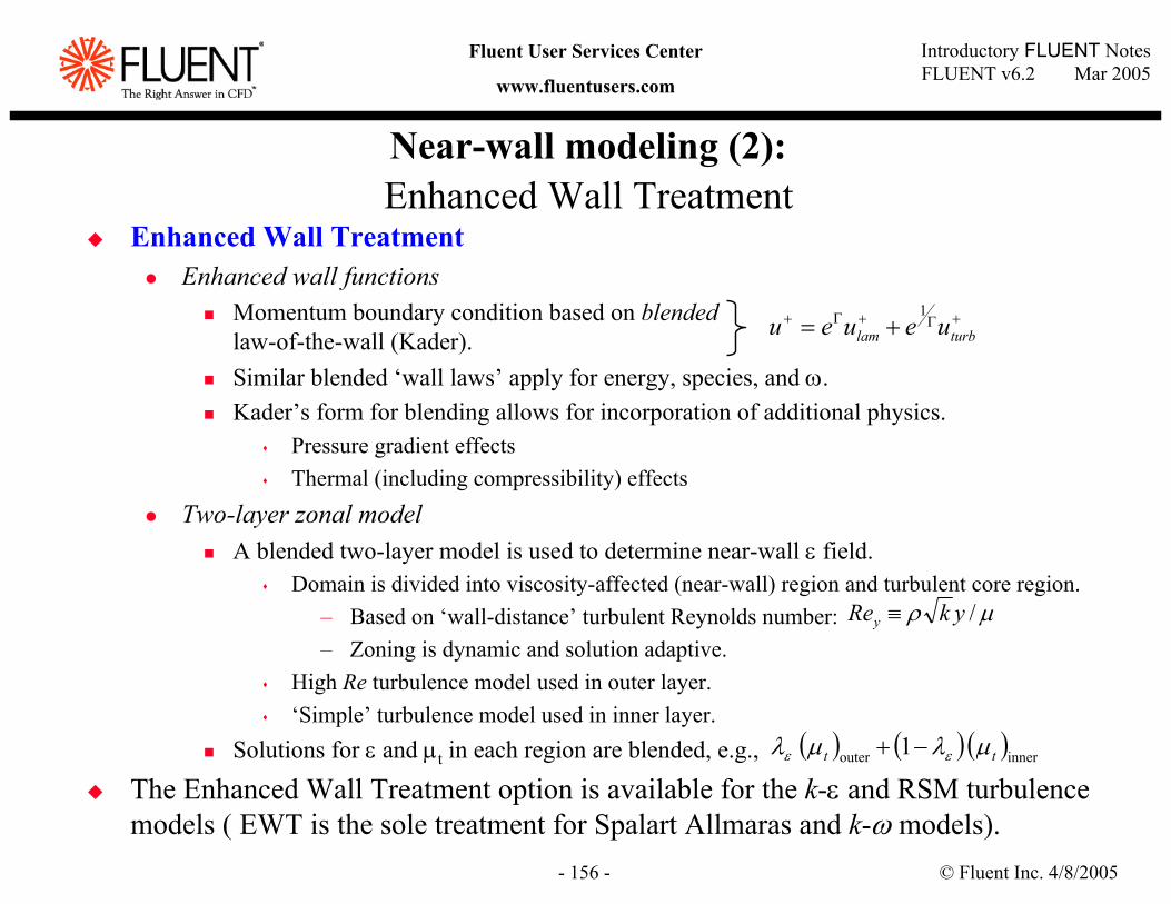
© Fluent Inc. 4/8/2005- 156 -



www.fluentusers.com

Near-wall modeling (2):Enhanced Wall Treatment

Enhanced Wall TreatmentEnhanced wall functions

Momentum boundary condition based on blendedlaw-of-the-wall (Kader).Similar blended ‘wall laws’ apply for energy, species, and ω.Kader’s form for blending allows for incorporation of additional physics.

Pressure gradient effects Thermal (including compressibility) effects

Two-layer zonal modelA blended two-layer model is used to determine near-wall ε field.

Domain is divided into viscosity-affected (near-wall) region and turbulent core region.– Based on ‘wall-distance’ turbulent Reynolds number:– Zoning is dynamic and solution adaptive.

High Re turbulence model used in outer layer.‘Simple’ turbulence model used in inner layer.

Solutions for ε and µt in each region are blended, e.g.,

The Enhanced Wall Treatment option is available for the k-ε and RSM turbulence models ( EWT is the sole treatment for Spalart Allmaras and k-ω models).

µρ /ykRey ≡

+Γ+Γ+ += turblam ueueu1

( ) ( ) ( )innerouter 1 tt µλµλ εε −+

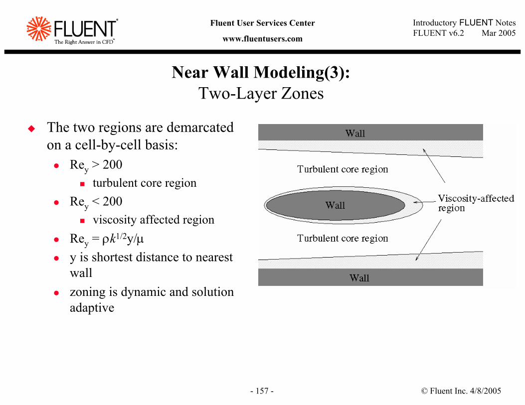
© Fluent Inc. 4/8/2005- 157 -



www.fluentusers.com

The two regions are demarcated on a cell-by-cell basis:

Rey > 200turbulent core region

Rey < 200viscosity affected region

Rey = ρk1/2y/µy is shortest distance to nearest wallzoning is dynamic and solution adaptive

Near Wall Modeling(3):Two-Layer Zones

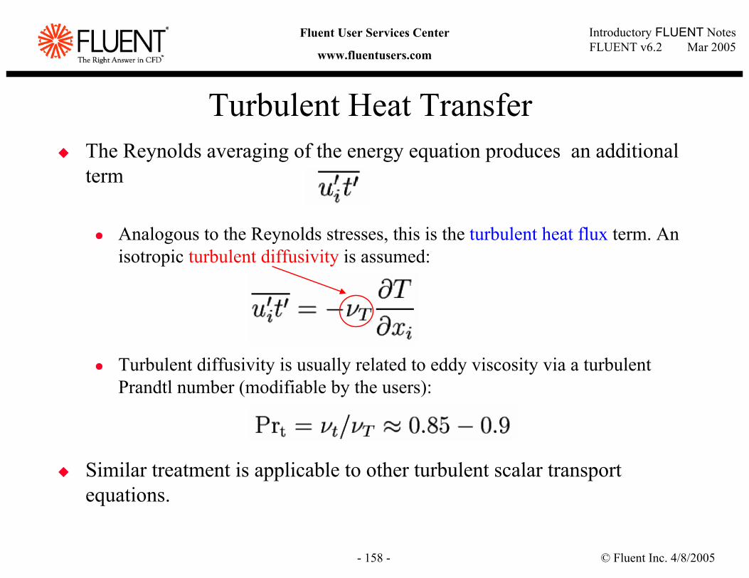
© Fluent Inc. 4/8/2005- 158 -



www.fluentusers.com

Turbulent Heat TransferThe Reynolds averaging of the energy equation produces an additional term

Analogous to the Reynolds stresses, this is the turbulent heat flux term. An isotropic turbulent diffusivity is assumed:

Turbulent diffusivity is usually related to eddy viscosity via a turbulent Prandtl number (modifiable by the users):

Similar treatment is applicable to other turbulent scalar transport equations.

© Fluent Inc. 4/8/2005- 159 -



www.fluentusers.com

Menter’s SST k-ω Model Background

Many people, including Menter (1994), have noted that:k-ω model has many good attributes and perform much better than k-ε models for boundary layer flows.Wilcox’ original k-ω model is overly sensitive to the freestreamvalue (BC) of ω, while k-ε model is not prone to such problem.Most two-equation models, including k-ε models, over-predict turbulent stresses in the wake (velocity-defect) region, which leads to poor performance of the models for boundary layers under adverse pressure gradient and separated flows.

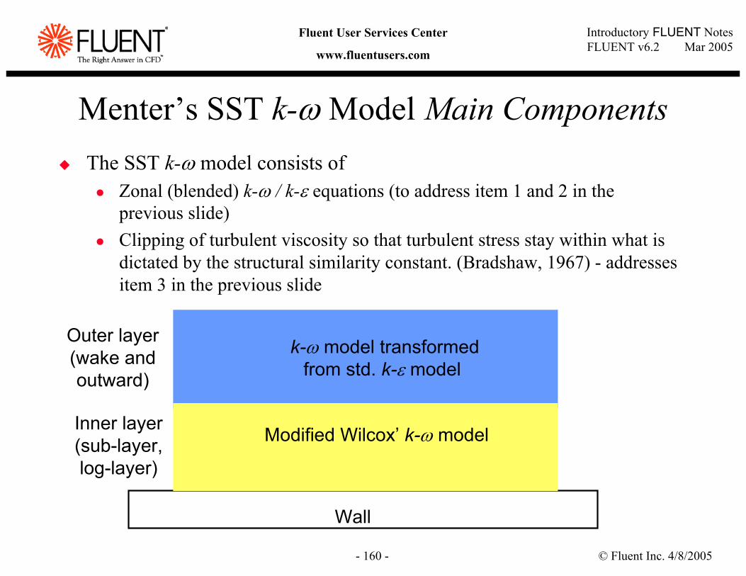
© Fluent Inc. 4/8/2005- 160 -



www.fluentusers.com

Menter’s SST k-ω Model Main ComponentsThe SST k-ω model consists of

Zonal (blended) k-ω / k-ε equations (to address item 1 and 2 in the previous slide)Clipping of turbulent viscosity so that turbulent stress stay within what is dictated by the structural similarity constant. (Bradshaw, 1967) - addresses item 3 in the previous slide

Inner layer (sub-layer, log-layer) Wilcox’ original k-ω model

ε

εl

23

k=

Wall

Outer layer (wake and outward)

k-ω model transformed from std. k-ε model

Modified Wilcox’ k-ω model

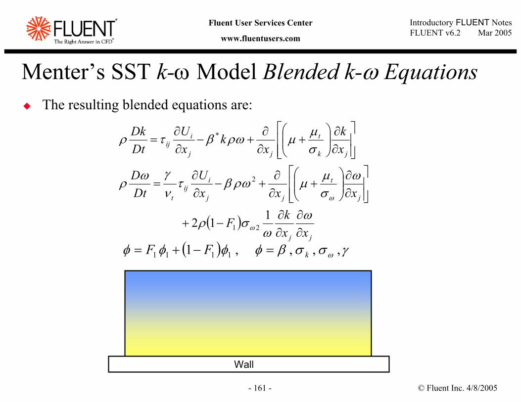
© Fluent Inc. 4/8/2005- 161 -



www.fluentusers.com

Menter’s SST k-ω Model Blended k-ω EquationsThe resulting blended equations are:

Wall

( )jj

j

t

jj

iij

t

jk

t

jj

iij

xxkF

xxxU

DtD

xk

xk

xU

DtDk

∂∂

∂∂

−+

∂∂

+

∂∂

+−∂∂

=

∂∂

+

∂∂

+−∂∂

=

ωω

σρ

ωσµµωρβτ

νγωρ

σµµωρβτρ

ω

ω

112 21

2

*

( ) γσσβφφφφ ω ,,,,1 1111 kFF =−+=

© Fluent Inc. 4/8/2005- 162 -



www.fluentusers.com

V2F Turbulence ModelA model developed by Paul Durbin’s group at Stanford:

Durbin suggests that the wall-normal fluctuations are responsible for the near-wall damping of the eddy viscosityRequires two additional transport equations for and a relaxation function f to be solved together with k and ε Eddy viscosity model is instead of

Promising results for many 3-D low-Re boundary-layer flows. For example, excellent predictions for heat transfer in jet impingementand separated flows, where k-ε models fail miserably.But it is a member of the EVM---same limitations still apply.V2F is an embedded add-on functionality in Fluent 6.x which requires a separate license from Cascade Technologies (www.turbulentflow.com)

© Fluent Inc. 4/8/2005- 163 -



www.fluentusers.com

Initial Velocity Field for LES/DES

Initial condition for velocity field does not affect statistically stationary solutionsHowever, starting LES with a realistic turbulent velocity field can substantially shorten the simulation time to get to statistically stationary stateThe spectral synthesizer can be used to superimpose turbulent velocity on top of the mean velocity field

Uses steady-state RANS ( k-ε, k-ω, RSM, etc.) solutions as inputs to the spectral synthesizerAccessible via a TUI command:/solve/initialize/init-instantaneous-vel

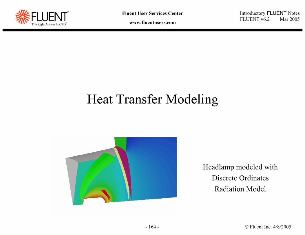
© Fluent Inc. 4/8/2005- 164 -



www.fluentusers.com

Heat Transfer Modeling

Headlamp modeled withDiscrete OrdinatesRadiation Model

© Fluent Inc. 4/8/2005- 165 -



www.fluentusers.com

OutlineIntroductionConjugate Heat TransferNatural ConvectionRadiationPeriodic Heat Transfer

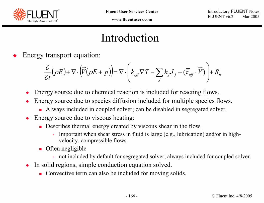
© Fluent Inc. 4/8/2005- 166 -



www.fluentusers.com

IntroductionEnergy transport equation:

Energy source due to chemical reaction is included for reacting flows.Energy source due to species diffusion included for multiple species flows.

Always included in coupled solver; can be disabled in segregated solver.Energy source due to viscous heating:

Describes thermal energy created by viscous shear in the flow.Important when shear stress in fluid is large (e.g., lubrication) and/or in high-velocity, compressible flows.

Often negligiblenot included by default for segregated solver; always included for coupled solver.

In solid regions, simple conduction equation solved.Convective term can also be included for moving solids.

( ) ( )( ) hj

effjjeff SVJhTkpEVEt

+

⋅+−∇⋅∇=+⋅∇+

∂∂ ∑ )(τρρ

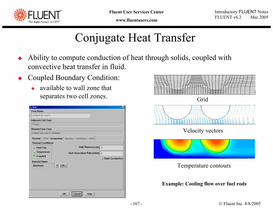
© Fluent Inc. 4/8/2005- 167 -



www.fluentusers.com

Conjugate Heat TransferAbility to compute conduction of heat through solids, coupled with convective heat transfer in fluid.Coupled Boundary Condition:

available to wall zone that separates two cell zones. Grid

Temperature contours

Velocity vectors

Example: Cooling flow over fuel rods

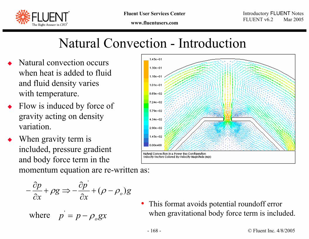
© Fluent Inc. 4/8/2005- 168 -



www.fluentusers.com

Natural Convection - IntroductionNatural convection occurswhen heat is added to fluidand fluid density varieswith temperature.Flow is induced by force ofgravity acting on densityvariation.When gravity term isincluded, pressure gradientand body force term in themomentum equation are re-written as:

gxpg

xp

o )('

ρρρ −+∂∂

−⇒+∂∂

−

where gxpp oρ−='• This format avoids potential roundoff error

when gravitational body force term is included.

© Fluent Inc. 4/8/2005- 169 -



www.fluentusers.com

Natural Convection – the Boussinesq ModelBoussinesq model assumes the fluid density is uniform

Except for the body force term in the momentum equation along the direction of gravity, we have:

Valid when density variations are small (i.e., small variations in T).It provides faster convergence for many natural-convection flows than by using fluid density as function of temperature.

Constant density assumptions reduces non-linearity.Suitable when density variations are small.Cannot be used together with species transport or reacting flows.

Natural convection problems inside closed domains:For steady-state solver, Boussinesq model must be used.

The constant density, ρo, properly specifies the mass of the domain.For unsteady solver, Boussinesq model or ideal-gas law can be used.

Initial conditions define mass in the domain.

( ) ( )ρ ρ ρ β− = − −0 0 0g T T g

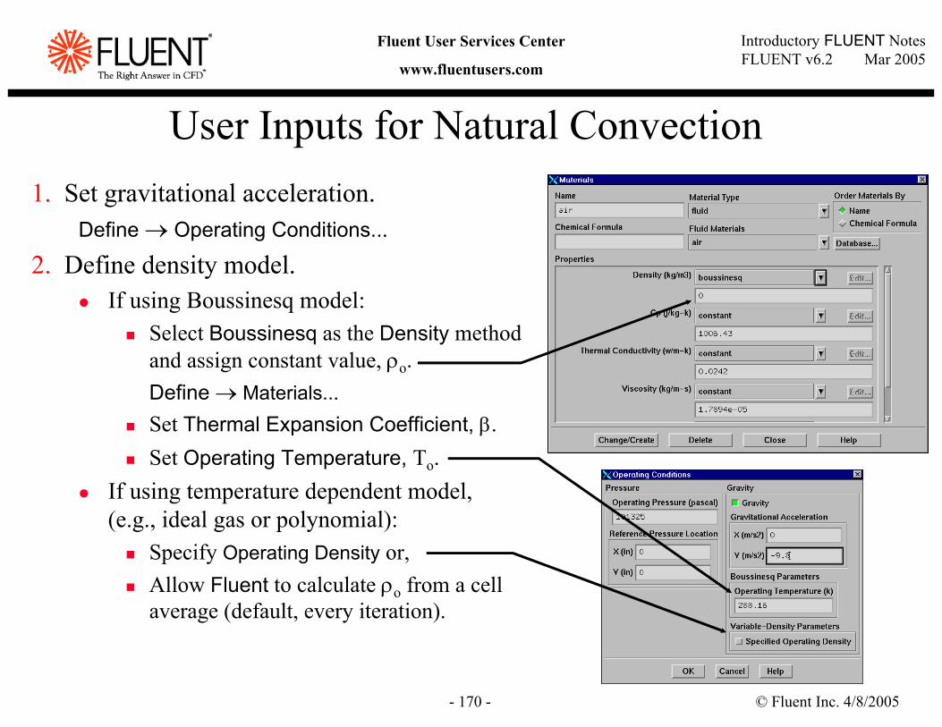
© Fluent Inc. 4/8/2005- 170 -



www.fluentusers.com

User Inputs for Natural Convection1. Set gravitational acceleration.

Define → Operating Conditions...2. Define density model.

If using Boussinesq model:Select Boussinesq as the Density method and assign constant value, ρo.Define → Materials...Set Thermal Expansion Coefficient, β.Set Operating Temperature, To.

If using temperature dependent model, (e.g., ideal gas or polynomial):

Specify Operating Density or,Allow Fluent to calculate ρo from a cell average (default, every iteration).

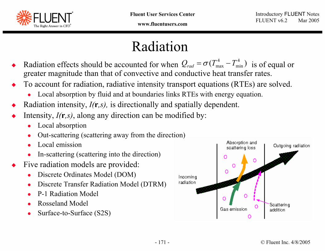
© Fluent Inc. 4/8/2005- 171 -



www.fluentusers.com

RadiationRadiation effects should be accounted for when is of equal or greater magnitude than that of convective and conductive heat transfer rates.To account for radiation, radiative intensity transport equations (RTEs) are solved.

Local absorption by fluid and at boundaries links RTEs with energy equation.Radiation intensity, I(r,s), is directionally and spatially dependent.Intensity, I(r,s), along any direction can be modified by:

Local absorptionOut-scattering (scattering away from the direction)Local emissionIn-scattering (scattering into the direction)

Five radiation models are provided:Discrete Ordinates Model (DOM)Discrete Transfer Radiation Model (DTRM)P-1 Radiation ModelRosseland ModelSurface-to-Surface (S2S)

)( 4min

4max TTQrad −= σ

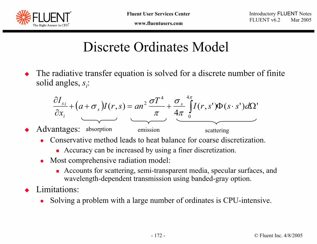
© Fluent Inc. 4/8/2005- 172 -



www.fluentusers.com

Discrete Ordinates Model

The radiative transfer equation is solved for a discrete number of finite solid angles, si:

Advantages:Conservative method leads to heat balance for coarse discretization.

Accuracy can be increased by using a finer discretization.Most comprehensive radiation model:

Accounts for scattering, semi-transparent media, specular surfaces, and wavelength-dependent transmission using banded-gray option.

Limitations: Solving a problem with a large number of ordinates is CPU-intensive.

( ) ')'()',(4

),(4

0

42 Ω⋅Φ+=++

∂∂

∫ dsssrITansrIaxI s

si

isπ

πσ

πσσ

absorption emission scattering

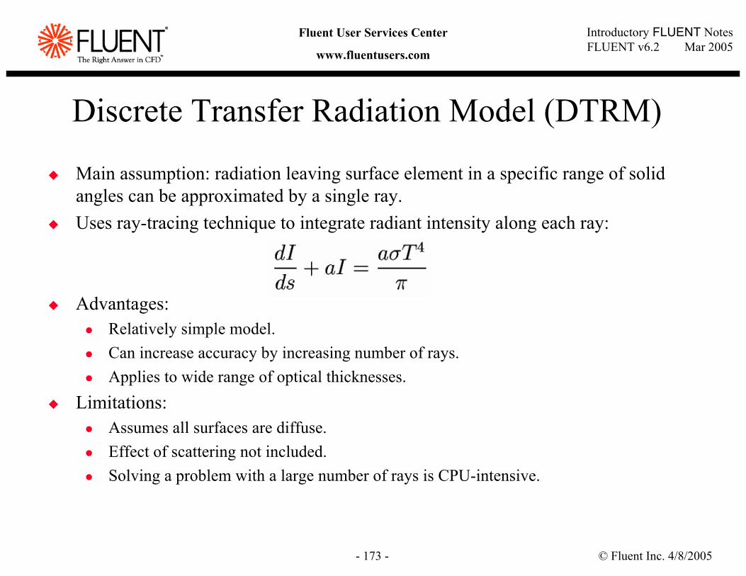
© Fluent Inc. 4/8/2005- 173 -



www.fluentusers.com

Discrete Transfer Radiation Model (DTRM)

Main assumption: radiation leaving surface element in a specific range of solid angles can be approximated by a single ray.Uses ray-tracing technique to integrate radiant intensity along each ray:

Advantages:Relatively simple model.Can increase accuracy by increasing number of rays.Applies to wide range of optical thicknesses.

Limitations:Assumes all surfaces are diffuse. Effect of scattering not included.Solving a problem with a large number of rays is CPU-intensive.

© Fluent Inc. 4/8/2005- 174 -



www.fluentusers.com

P-1 ModelMain assumption: Directional dependence in RTE is integrated out, resulting in a diffusion equation for incident radiation. Advantages:

Radiative transfer equation easy to solve with little CPU demand. Includes effect of scattering.

Effects of particles, droplets, and soot can be included.Works reasonably well for combustion applications where optical thickness is large.

Limitations:Assumes all surfaces are diffuse. May result in loss of accuracy, depending on complexity of geometry, if optical thickness is small.Tends to overpredict radiative fluxes from localized heat sources or sinks.

© Fluent Inc. 4/8/2005- 175 -



www.fluentusers.com

Surface-to-Surface Radiation ModelThe S2S radiation model can be used for modeling enclosure radiativetransfer without participating media.

e.g., spacecraft heat rejection system, solar collector systems, radiative space heaters, and automotive underhood coolingView-factor based modelNon-participating media is assumed.

Limitations: The S2S model assumes that all surfaces are diffuse. The implementation assumes gray radiation. Storage and memory requirements increase very rapidly as the number of surface faces increases.

Memory requirements can be reduced by using clusters of surface faces.Clustering does not work with sliding meshes or hanging nodes.

Not to be used with periodic or symmetry boundary conditions. Cannot be used for models with multiple enclosures geometry.

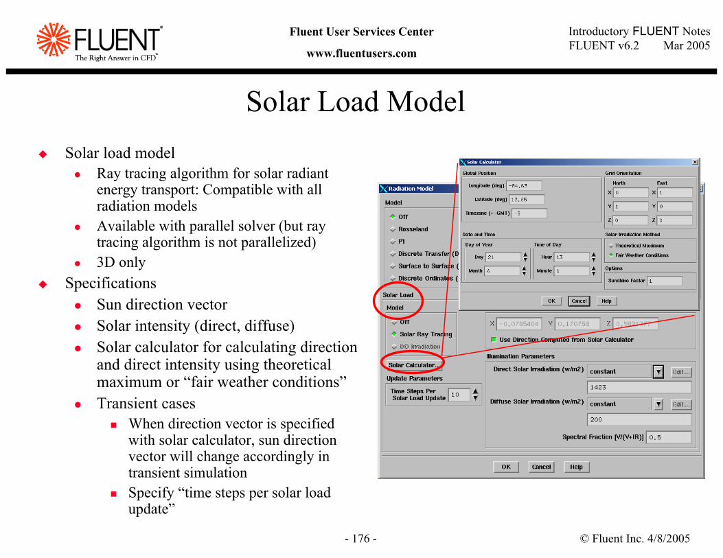
© Fluent Inc. 4/8/2005- 176 -



www.fluentusers.com

Solar Load ModelSolar load model

Ray tracing algorithm for solar radiant energy transport: Compatible with all radiation modelsAvailable with parallel solver (but ray tracing algorithm is not parallelized)3D only

SpecificationsSun direction vectorSolar intensity (direct, diffuse)Solar calculator for calculating direction and direct intensity using theoretical maximum or “fair weather conditions”Transient cases

When direction vector is specified with solar calculator, sun direction vector will change accordingly in transient simulationSpecify “time steps per solar load update”

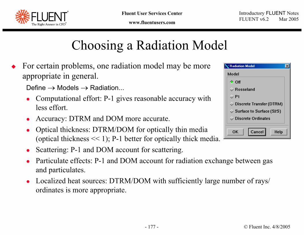
© Fluent Inc. 4/8/2005- 177 -



www.fluentusers.com

Choosing a Radiation ModelFor certain problems, one radiation model may be more appropriate in general.

Define → Models → Radiation...Computational effort: P-1 gives reasonable accuracy with less effort.Accuracy: DTRM and DOM more accurate.Optical thickness: DTRM/DOM for optically thin media (optical thickness << 1); P-1 better for optically thick media.Scattering: P-1 and DOM account for scattering.Particulate effects: P-1 and DOM account for radiation exchange between gas and particulates.Localized heat sources: DTRM/DOM with sufficiently large number of rays/ ordinates is more appropriate.

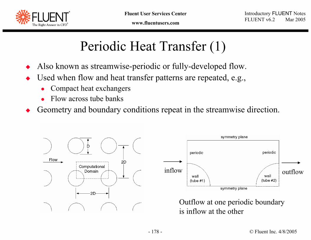
© Fluent Inc. 4/8/2005- 178 -



www.fluentusers.com

Periodic Heat Transfer (1)Also known as streamwise-periodic or fully-developed flow.Used when flow and heat transfer patterns are repeated, e.g.,

Compact heat exchangersFlow across tube banks

Geometry and boundary conditions repeat in the streamwise direction.

Outflow at one periodic boundary is inflow at the other

inflow outflow

© Fluent Inc. 4/8/2005- 179 -



www.fluentusers.com

Periodic Heat Transfer (2)

Temperature (and pressure) vary in the streamwise direction.Scaled temperature (and periodic pressure) is same at periodic boundaries. For fixed wall temperature problems, scaled temperature defined as:

Tb = suitably defined bulk temperatureCan also model flows with specified wall heat flux.

θ =−−

T TT T

wall

b wall

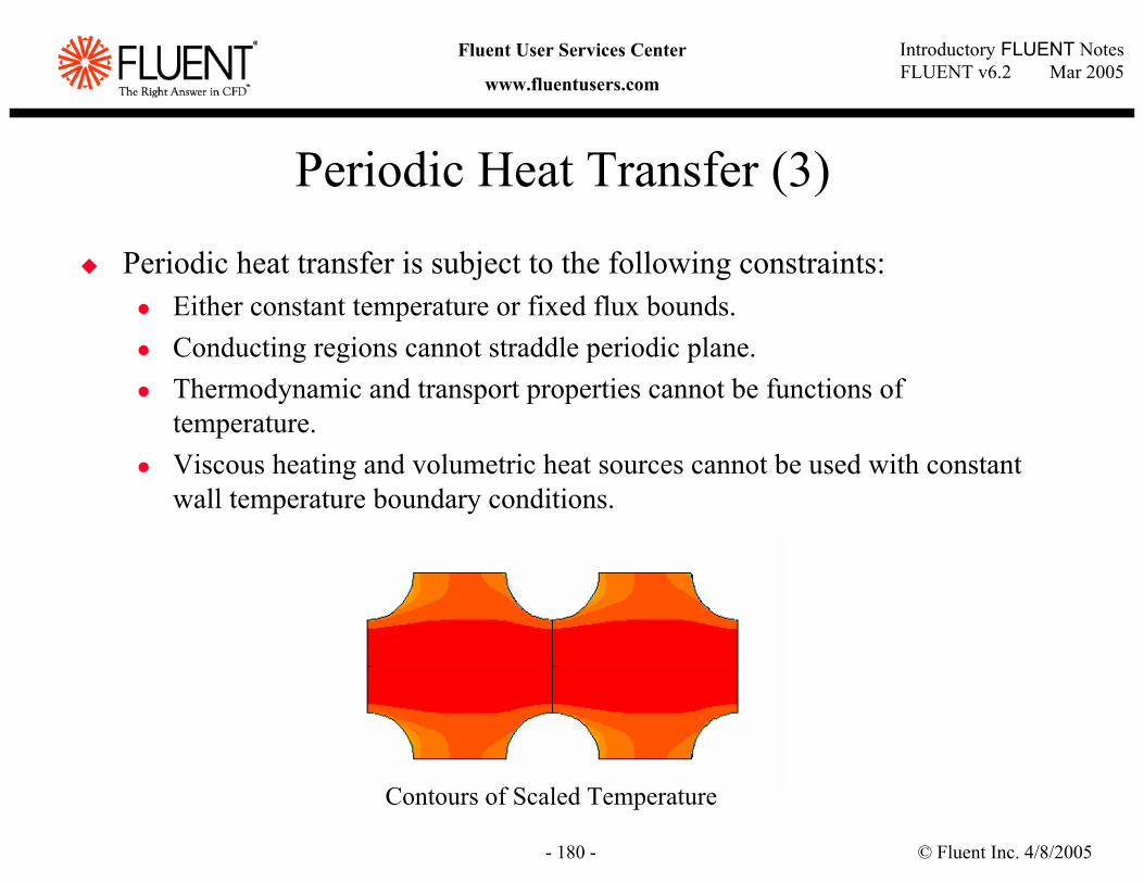
© Fluent Inc. 4/8/2005- 180 -



www.fluentusers.com

Periodic Heat Transfer (3)

Periodic heat transfer is subject to the following constraints:Either constant temperature or fixed flux bounds.Conducting regions cannot straddle periodic plane.Thermodynamic and transport properties cannot be functions of temperature.Viscous heating and volumetric heat sources cannot be used with constant wall temperature boundary conditions.

Contours of Scaled Temperature

© Fluent Inc. 4/8/2005- 181 -



www.fluentusers.com

Summary

Heat transfer modeling is available in all Fluent solvers.After activating heat transfer, you must provide:

Thermal conditions at walls and flow boundariesFluid properties for energy equation

Available heat transfer modeling options include:Species diffusion heat sourceCombustion heat sourceConjugate heat transferNatural convectionRadiationPeriodic heat transfer

© Fluent Inc. 4/8/2005- 182 -



www.fluentusers.com

User Defined Functions

© Fluent Inc. 4/8/2005- 183 -



www.fluentusers.com

IntroductionWhat is a User Defined Function?

A UDF is a routine (programmed by the user) written in C which can be dynamically linked with the solver.

Standard C functionse.g., trigonometric, exponential, control blocks, do-loops, file i/o, etc.

Pre-Defined MacrosAllows access to field variable, material property, and cell geometry data.

Why build UDF’s?Standard interface cannot be programmed to anticipate all needs.

Customization of boundary conditions, source terms, reaction rates, material properties, etc.Adjust functions (once per iteration)Execute on Demand functionsSolution Initialization

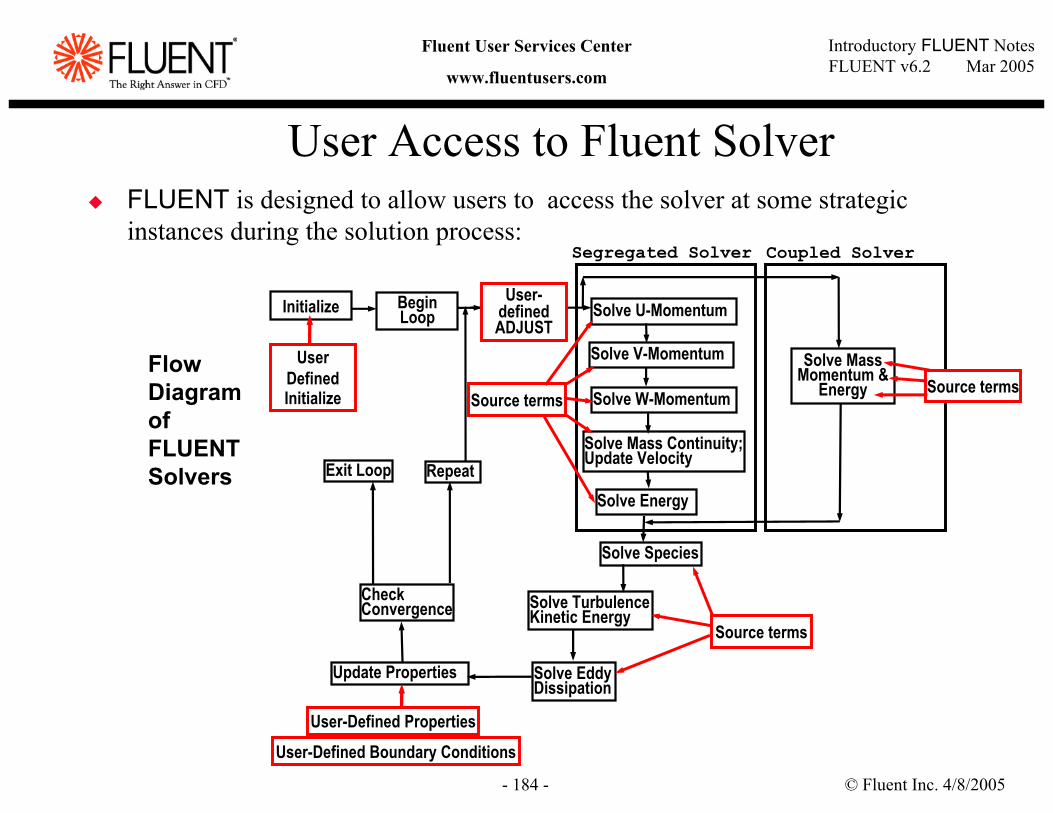
© Fluent Inc. 4/8/2005- 184 -



www.fluentusers.com

User Access to Fluent SolverFLUENT is designed to allow users to access the solver at some strategic instances during the solution process:

Flow Diagram of FLUENT Solvers

Segregated Solver Coupled Solver

Initialize Begin Loop

Exit Loop Repeat

Check Convergence

Update Properties Solve Eddy Dissipation

Solve Turbulence Kinetic Energy

Solve Species

Solve Energy

Solve Mass Continuity;Update Velocity

Solve U-Momentum

Solve V-Momentum

Solve W-Momentum

Solve Mass Momentum &

Energy

User-defined ADJUST

Source termsSource terms

Source terms

User Defined Initialize

User-Defined PropertiesUser-Defined Boundary Conditions

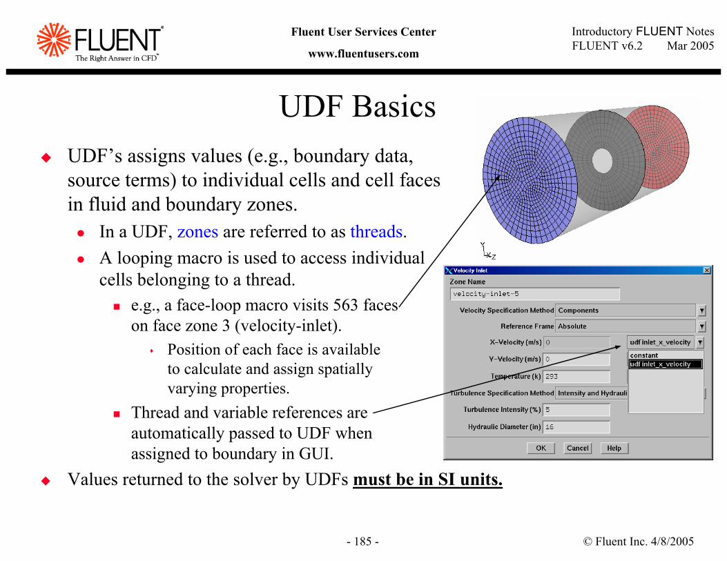
© Fluent Inc. 4/8/2005- 185 -



www.fluentusers.com

UDF BasicsUDF’s assigns values (e.g., boundary data, source terms) to individual cells and cell faces in fluid and boundary zones.

In a UDF, zones are referred to as threads.A looping macro is used to access individualcells belonging to a thread.

e.g., a face-loop macro visits 563 faces on face zone 3 (velocity-inlet).

Position of each face is availableto calculate and assign spatially varying properties.

Thread and variable references are automatically passed to UDF when assigned to boundary in GUI.

Values returned to the solver by UDFs must be in SI units.

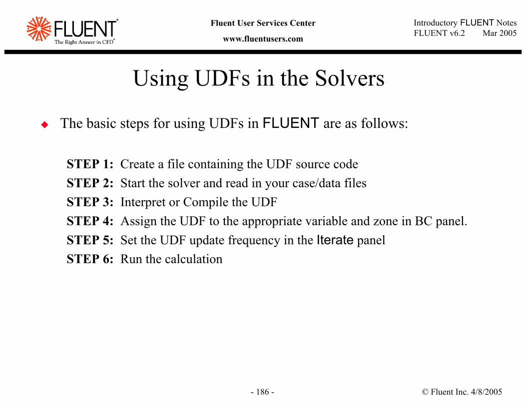
© Fluent Inc. 4/8/2005- 186 -



www.fluentusers.com

Using UDFs in the Solvers

The basic steps for using UDFs in FLUENT are as follows:

STEP 1: Create a file containing the UDF source codeSTEP 2: Start the solver and read in your case/data filesSTEP 3: Interpret or Compile the UDFSTEP 4: Assign the UDF to the appropriate variable and zone in BC panel.STEP 5: Set the UDF update frequency in the Iterate panelSTEP 6: Run the calculation

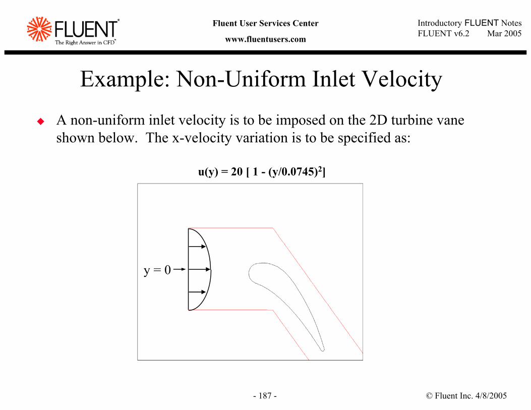
© Fluent Inc. 4/8/2005- 187 -



www.fluentusers.com

Example: Non-Uniform Inlet VelocityA non-uniform inlet velocity is to be imposed on the 2D turbine vane shown below. The x-velocity variation is to be specified as:

u(y) = 20 [ 1 - (y/0.0745)2]

y = 0

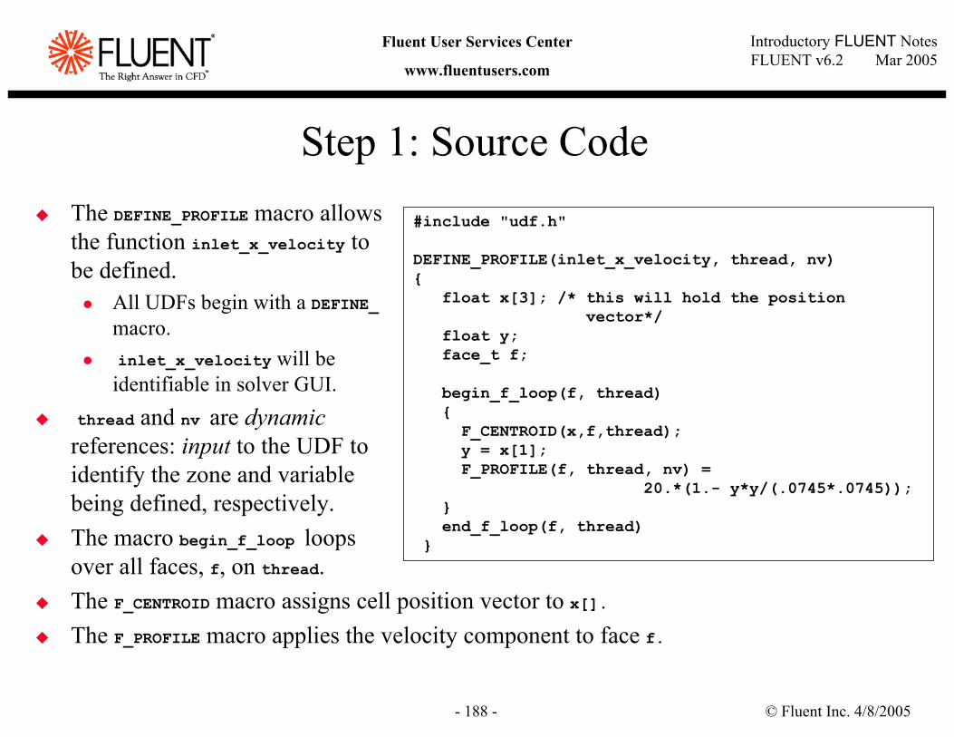
© Fluent Inc. 4/8/2005- 188 -



www.fluentusers.com

Step 1: Source CodeThe DEFINE_PROFILE macro allowsthe function inlet_x_velocity tobe defined.

All UDFs begin with a DEFINE_macro.inlet_x_velocity will be identifiable in solver GUI.

thread and nv are dynamicreferences: input to the UDF toidentify the zone and variablebeing defined, respectively.The macro begin_f_loop loops over all faces, f, on thread.The F_CENTROID macro assigns cell position vector to x[]. The F_PROFILE macro applies the velocity component to face f.

#include "udf.h"

DEFINE_PROFILE(inlet_x_velocity, thread, nv)

float x[3]; /* this will hold the position vector*/

float y;face_t f;

begin_f_loop(f, thread)

F_CENTROID(x,f,thread);y = x[1];F_PROFILE(f, thread, nv) =

20.*(1.- y*y/(.0745*.0745));end_f_loop(f, thread)

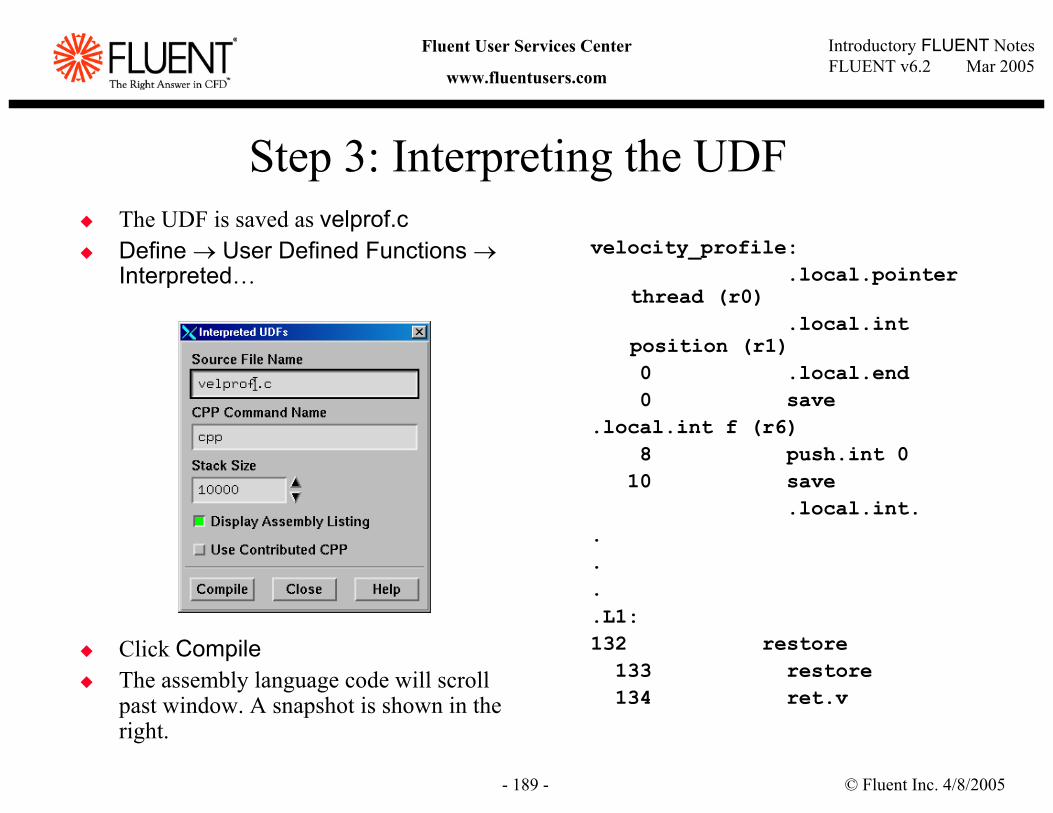
© Fluent Inc. 4/8/2005- 189 -



www.fluentusers.com

Step 3: Interpreting the UDFThe UDF is saved as velprof.cDefine → User Defined Functions →Interpreted…

Click CompileThe assembly language code will scroll past window. A snapshot is shown in the right.

velocity_profile:.local.pointer

thread (r0).local.int

position (r1)0 .local.end0 save

.local.int f (r6)8 push.int 010 save

.local.int.....L1:132 restore133 restore134 ret.v

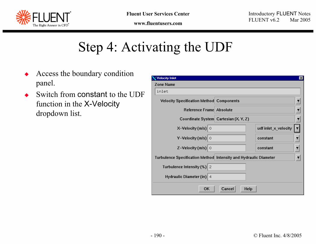
© Fluent Inc. 4/8/2005- 190 -



www.fluentusers.com

Step 4: Activating the UDF

Access the boundary condition panel.Switch from constant to the UDF function in the X-Velocitydropdown list.

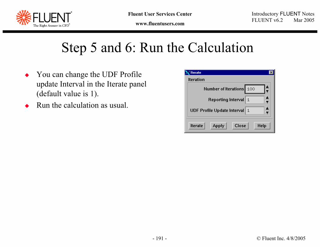
© Fluent Inc. 4/8/2005- 191 -



www.fluentusers.com

Step 5 and 6: Run the Calculation

You can change the UDF Profile update Interval in the Iterate panel (default value is 1).Run the calculation as usual.

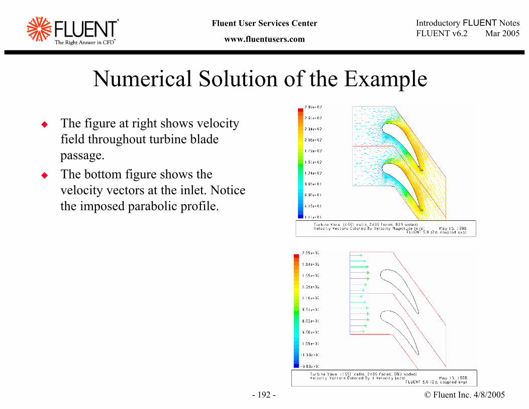
© Fluent Inc. 4/8/2005- 192 -



www.fluentusers.com

Numerical Solution of the Example

The figure at right shows velocity field throughout turbine blade passage.The bottom figure shows the velocity vectors at the inlet. Notice the imposed parabolic profile.

© Fluent Inc. 4/8/2005- 193 -



www.fluentusers.com

MacrosMacros are pre-defined (Fluent) functions:

DEFINE_ macros allows definitions of UDF functionality.Variable access macros allow access to field variables and cell information.Utility macros provide looping capabilities, thread identification, vector and numerous other functions.

Macros are defined in header files.The udf.h header file must be included in your source code.

#include “udf.h”

The header files must be accessible in your path.Typically stored in Fluent.Inc/src/ directory.

A list of often used macros is provided in the UDF User’s Guide.

Help → More Documentation

© Fluent Inc. 4/8/2005- 194 -



www.fluentusers.com

DEFINE MacrosAny UDF you write must begin with a DEFINE macro:

18 ‘general purpose’ macros and 13 DPM and multiphase related macros (not listed):

DEFINE_ADJUST(name,domain); general purpose UDF called every iterationDEFINE_INIT(name,domain); UDF used to initialize field variablesDEFINE_ON_DEMAND(name); defines an ‘execute-on-demand’ functionDEFINE_RW_FILE(name,fp); customize reads/writes to case/data filesDEFINE_PROFILE(name,thread,index); defines boundary profilesDEFINE_SOURCE(name,cell,thread,dS,index); defines source termsDEFINE_HEAT_FLUX(name,face,thread,c0,t0,cid,cir); defines heat fluxDEFINE_PROPERTY(name,cell,thread); defines material propertiesDEFINE_DIFFUSIVITY(name,cell,thread,index); defines UDS and species diffusivitiesDEFINE_UDS_FLUX(name,face,thread,index); defines UDS flux termsDEFINE_UDS_UNSTEADY(name,cell,thread,index,apu,su); defines UDS transient termsDEFINE_SR_RATE(name,face,thread,r,mw,yi,rr); defines surface reaction ratesDEFINE_VR_RATE(name,cell,thread,r,mw,yi,rr,rr_t); defines vol. reaction ratesDEFINE_SCAT_PHASE_FUNC(name,cell,face); defines scattering phase function for DOMDEFINE_DELTAT(name,domain); defines variable time step size for unsteady problemsDEFINE_TURBULENT_VISCOSITY(name,cell,thread); defines procedure for calculating turbulent viscosityDEFINE_TURB_PREMIX_SOURCE(name,cell,thread,turbflamespeed,source); defines turb. flame speedDEFINE_NOX_RATE(name,cell,thread,nox); defines NOx production and destruction rates

© Fluent Inc. 4/8/2005- 195 -



www.fluentusers.com

Some Thread and Looping Utility Macros

cell_t c; defines a cellface_t f; defines a faceThread *t; pointer to a threadDomain *d; pointer to collection of all threads

thread_loop_c(t, d) loop that steps through all cell threads in domainthread_loop_f(t, d) loop that steps through all face threads in domainbegin_c_loop(c, t) end_c_loop(c, t) loop that steps through all cells in a threadbegin_f_loop(f, t) end_f_loop(f, t) loop that steps through all faces in a threadc_face_loop(c, t, n) loop that steps through all faces of a cell

Thread *tf = Lookup_Thread(domain, ID); return thread pointer of integer ID of zoneTHREAD_ID(tf); returns zone integer ID of thread pointer

Code enclosed in is executed in loop.

Specialized variable types used for referencing.

© Fluent Inc. 4/8/2005- 196 -



www.fluentusers.com

Geometry and Time Macros

C_NNODES(c, t); returns nodes/cellC_NFACES(c, t); returns faces/cellF_NNODES(f, t); returns nodes/faceC_CENTROID(x, c, t); returns coordinates of cell centroid in array x[]F_CENTROID(x, f, t); returns coordinates of face centroid in array x[]F_AREA(A, f, t); returns area vector in array A[]C_VOLUME(c, t); returns cell volume C_VOLUME_2D(c, t); returns cell volume for axisymmetric domain

real flow_time(); returns actual timeint time_step; returns time step numberRP_Get_Real(“physical-time-step”); returns time step size

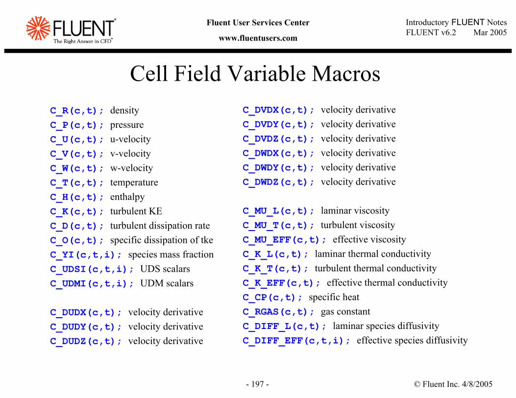
© Fluent Inc. 4/8/2005- 197 -



www.fluentusers.com

Cell Field Variable MacrosC_R(c,t); densityC_P(c,t); pressureC_U(c,t); u-velocityC_V(c,t); v-velocityC_W(c,t); w-velocityC_T(c,t); temperatureC_H(c,t); enthalpyC_K(c,t); turbulent KEC_D(c,t); turbulent dissipation rateC_O(c,t); specific dissipation of tkeC_YI(c,t,i); species mass fractionC_UDSI(c,t,i); UDS scalarsC_UDMI(c,t,i); UDM scalars

C_DUDX(c,t); velocity derivativeC_DUDY(c,t); velocity derivativeC_DUDZ(c,t); velocity derivative

C_DVDX(c,t); velocity derivativeC_DVDY(c,t); velocity derivativeC_DVDZ(c,t); velocity derivativeC_DWDX(c,t); velocity derivativeC_DWDY(c,t); velocity derivativeC_DWDZ(c,t); velocity derivative

C_MU_L(c,t); laminar viscosityC_MU_T(c,t); turbulent viscosityC_MU_EFF(c,t); effective viscosityC_K_L(c,t); laminar thermal conductivityC_K_T(c,t); turbulent thermal conductivityC_K_EFF(c,t); effective thermal conductivityC_CP(c,t); specific heatC_RGAS(c,t); gas constantC_DIFF_L(c,t); laminar species diffusivityC_DIFF_EFF(c,t,i); effective species diffusivity

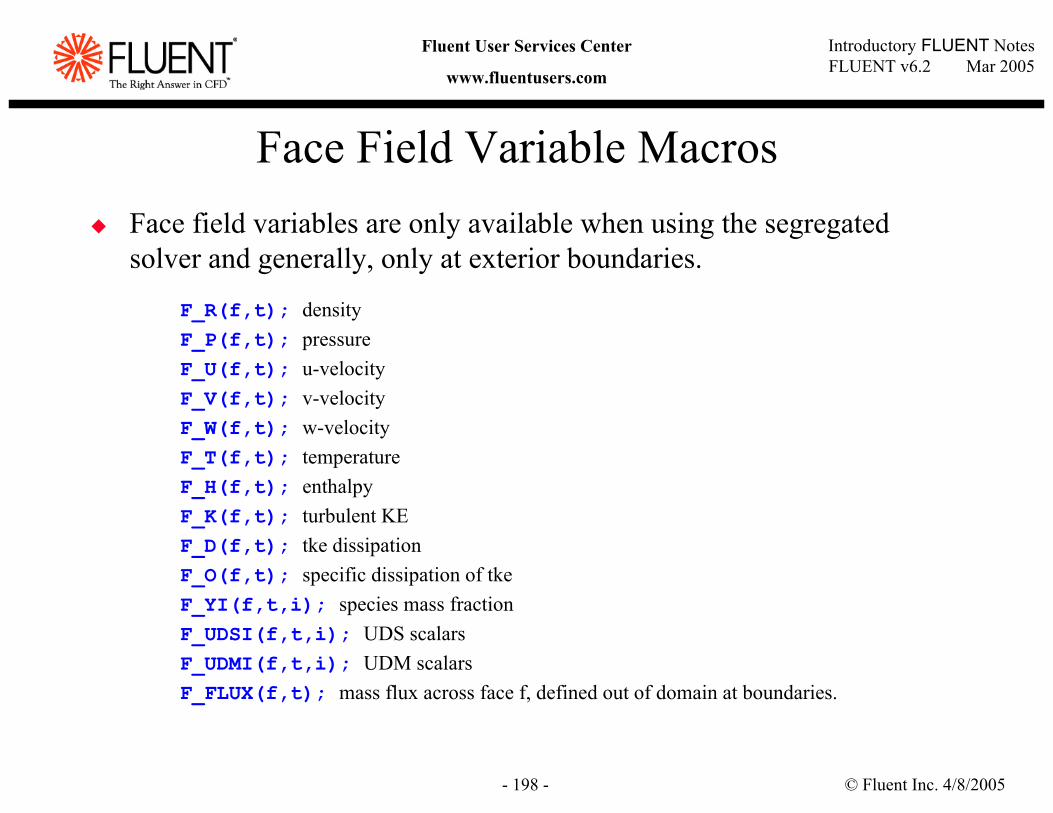
© Fluent Inc. 4/8/2005- 198 -



www.fluentusers.com

Face Field Variable Macros

F_R(f,t); densityF_P(f,t); pressureF_U(f,t); u-velocityF_V(f,t); v-velocityF_W(f,t); w-velocityF_T(f,t); temperatureF_H(f,t); enthalpyF_K(f,t); turbulent KEF_D(f,t); tke dissipationF_O(f,t); specific dissipation of tkeF_YI(f,t,i); species mass fractionF_UDSI(f,t,i); UDS scalarsF_UDMI(f,t,i); UDM scalarsF_FLUX(f,t); mass flux across face f, defined out of domain at boundaries.

Face field variables are only available when using the segregated solver and generally, only at exterior boundaries.

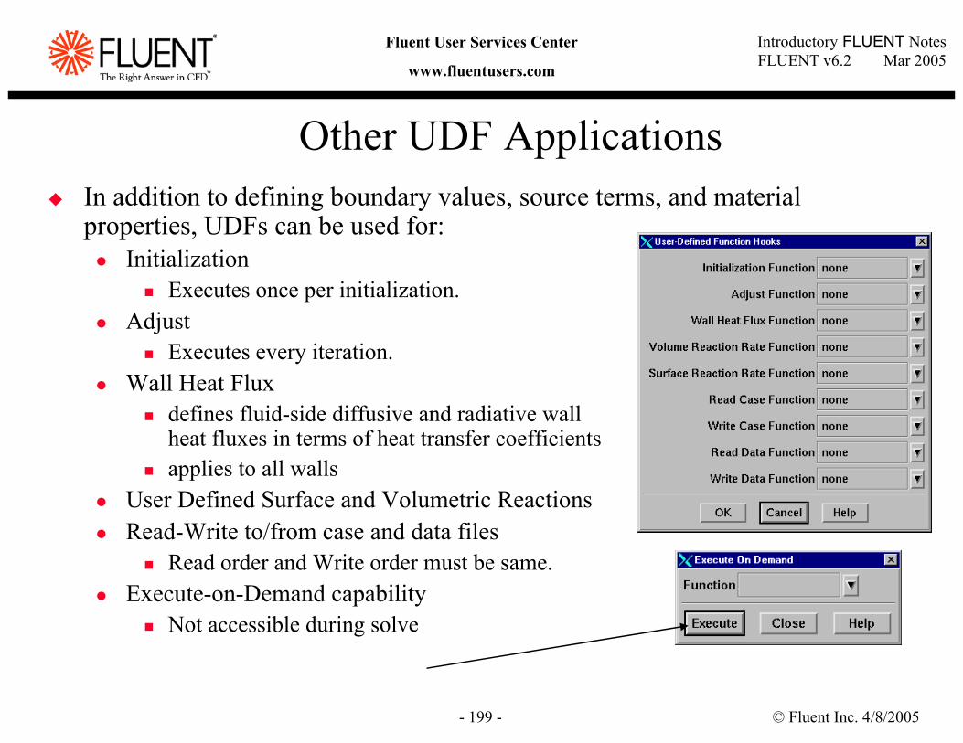
© Fluent Inc. 4/8/2005- 199 -



www.fluentusers.com

Other UDF ApplicationsIn addition to defining boundary values, source terms, and material properties, UDFs can be used for:

InitializationExecutes once per initialization.

AdjustExecutes every iteration.

Wall Heat Fluxdefines fluid-side diffusive and radiative wall heat fluxes in terms of heat transfer coefficientsapplies to all walls

User Defined Surface and Volumetric ReactionsRead-Write to/from case and data files

Read order and Write order must be same.Execute-on-Demand capability

Not accessible during solve

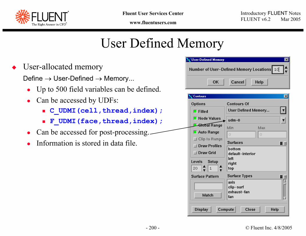
© Fluent Inc. 4/8/2005- 200 -



www.fluentusers.com

User Defined MemoryUser-allocated memoryDefine → User-Defined → Memory...

Up to 500 field variables can be defined.Can be accessed by UDFs:

C_UDMI(cell,thread,index);F_UDMI(face,thread,index);

Can be accessed for post-processing.Information is stored in data file.

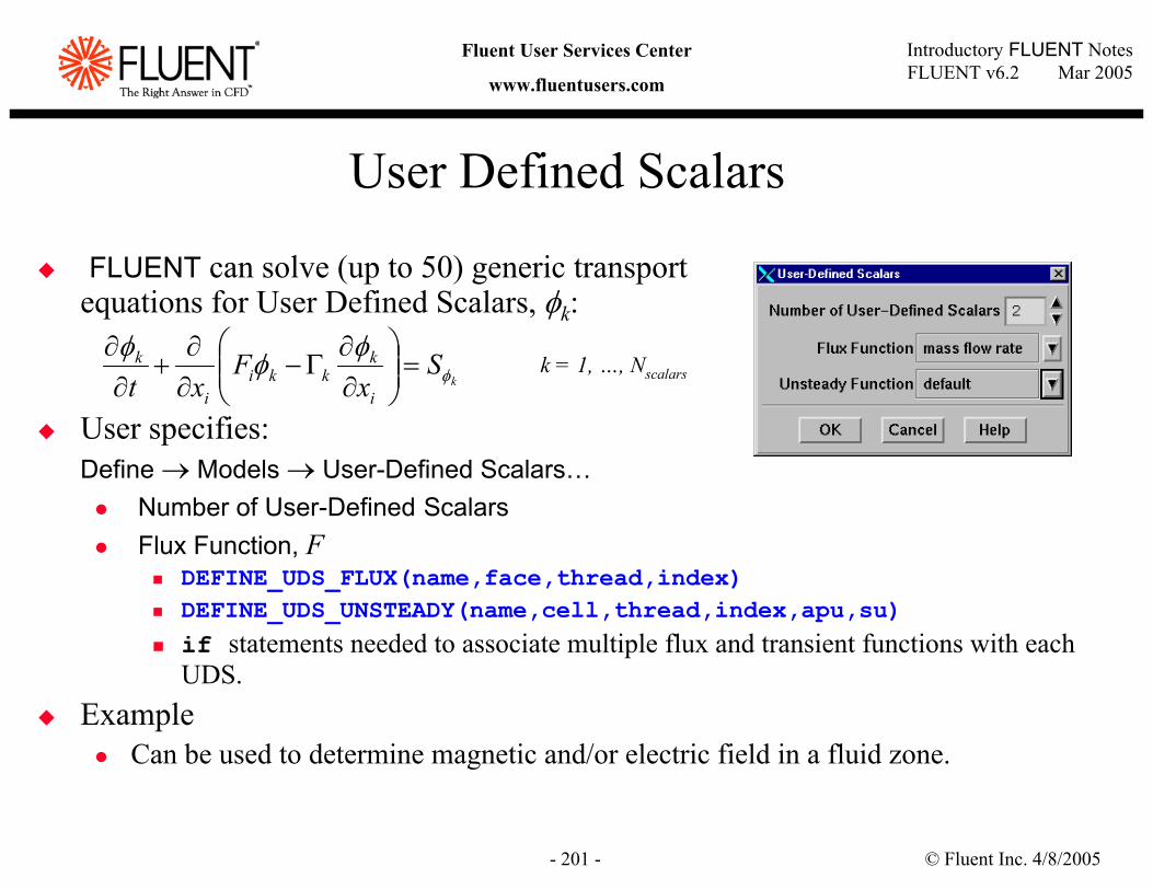
© Fluent Inc. 4/8/2005- 201 -



www.fluentusers.com

User Defined Scalars

FLUENT can solve (up to 50) generic transportequations for User Defined Scalars, φk:

User specifies:Define → Models → User-Defined Scalars…

Number of User-Defined ScalarsFlux Function, F

DEFINE_UDS_FLUX(name,face,thread,index)DEFINE_UDS_UNSTEADY(name,cell,thread,index,apu,su)if statements needed to associate multiple flux and transient functions with each UDS.

ExampleCan be used to determine magnetic and/or electric field in a fluid zone.

kS

xF

xt i

kkki

i

kφ

φφφ=

∂∂

Γ−∂∂

+∂

∂k = 1, …, Nscalars

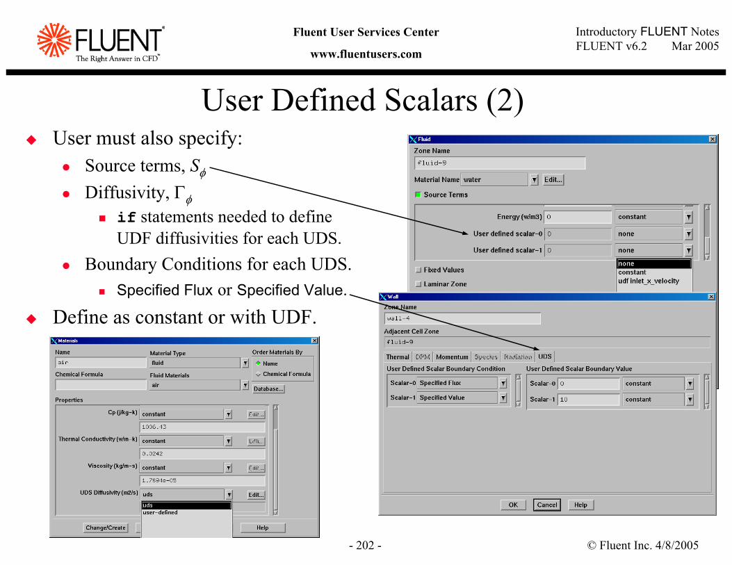
© Fluent Inc. 4/8/2005- 202 -



www.fluentusers.com

User Defined Scalars (2)User must also specify:

Source terms, Sφ

Diffusivity, Γφif statements needed to define UDF diffusivities for each UDS.

Boundary Conditions for each UDS.Specified Flux or Specified Value.

Define as constant or with UDF.

© Fluent Inc. 4/8/2005- 203 -



www.fluentusers.com

Interpreted vs. Compiled UDF’sFunctions can either be read in and interpreted at run time (as in the example) or compiled and grouped into a shared library that is linked with the standard FLUENT executable. Interpreted vs. compiled code

Interpreter -Interpreter is a large program that sits in the computer’s memory.Executes code on a “line by line” basis instantaneouslyAdvantages - does not need a separate compilerDisadvantage - slow and takes up space in memory

Compiler (refer to User’s Guide for instructions)-Code is translated “once” into machine language (object modules).Efficient way to run UDF’s. Uses MakefilesCreates “shared libraries” which are linked with the rest of the solverOvercomes interpreter limitations e.g. mixed mode arithmetic, structure references etc.

© Fluent Inc. 4/8/2005- 204 -



www.fluentusers.com

Supporting UDF’s

Because UDF’s can be very complicated, Fluent Inc. does not assume responsibility for the accuracy or stability of solutions obtained using UDFs that are user-generated.

Support will be limited to guidance related to communication between a UDF and the FLUENT solver.Other aspects of the UDF development process that include conceptual function design, implementation (writing C code), compilation and debugging of C source code, execution of the UDF, and function design verification will remain the responsibility of the UDF author.

Consulting option

© Fluent Inc. 4/8/2005- 205 -



www.fluentusers.com

Modeling Multiphase Flows

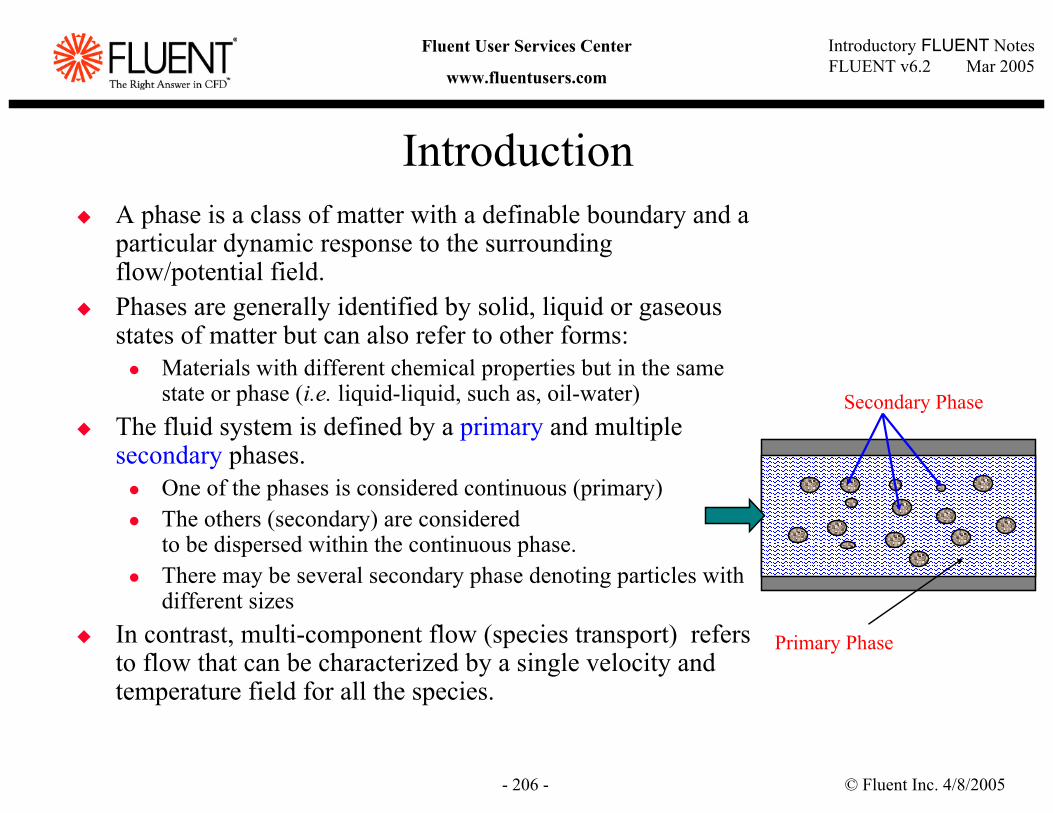
© Fluent Inc. 4/8/2005- 206 -



www.fluentusers.com

IntroductionA phase is a class of matter with a definable boundary and a particular dynamic response to the surrounding flow/potential field. Phases are generally identified by solid, liquid or gaseous states of matter but can also refer to other forms:

Materials with different chemical properties but in the same state or phase (i.e. liquid-liquid, such as, oil-water)

The fluid system is defined by a primary and multiple secondary phases.

One of the phases is considered continuous (primary)The others (secondary) are considered to be dispersed within the continuous phase.There may be several secondary phase denoting particles with different sizes

In contrast, multi-component flow (species transport) refers to flow that can be characterized by a single velocity and temperature field for all the species.

Primary Phase

Secondary Phase

© Fluent Inc. 4/8/2005- 207 -



www.fluentusers.com

Choosing a Multiphase Model

In order to select the appropriate model, users must know a priori the characteristics of the flow in terms of the following:

The flow regimeVolume loadingTurbulent or Laminar flowStokes number

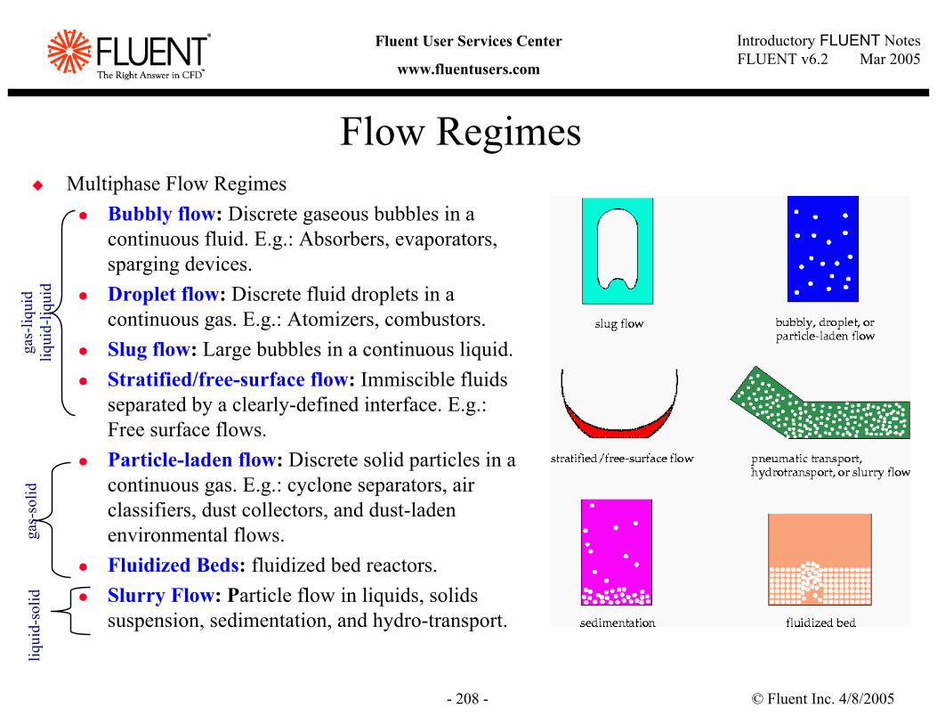
© Fluent Inc. 4/8/2005- 208 -



www.fluentusers.com

Flow RegimesMultiphase Flow Regimes

Bubbly flow: Discrete gaseous bubbles in a continuous fluid. E.g.: Absorbers, evaporators, sparging devices.Droplet flow: Discrete fluid droplets in a continuous gas. E.g.: Atomizers, combustors.Slug flow: Large bubbles in a continuous liquid.Stratified/free-surface flow: Immiscible fluids separated by a clearly-defined interface. E.g.: Free surface flows.Particle-laden flow: Discrete solid particles in a continuous gas. E.g.: cyclone separators, air classifiers, dust collectors, and dust-laden environmental flows.Fluidized Beds: fluidized bed reactors.Slurry Flow: Particle flow in liquids, solids suspension, sedimentation, and hydro-transport.

gas-

liqui

d liq

uid-

liqui

dga

s-so

lidliq

uid-

solid

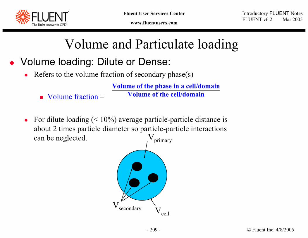
© Fluent Inc. 4/8/2005- 209 -



www.fluentusers.com

Volume and Particulate loadingVolume loading: Dilute or Dense:

Refers to the volume fraction of secondary phase(s)

Volume fraction =

For dilute loading (< 10%) average particle-particle distance is about 2 times particle diameter so particle-particle interactions can be neglected.

Volume of the phase in a cell/domainVolume of the cell/domain

Vsecondary Vcell

Vprimary

© Fluent Inc. 4/8/2005- 210 -



www.fluentusers.com

Turbulence modeling in Multiphase Flows

Turbulence modeling with multiphase flows can be challenging. Presently, single-phase models like k-ε or RSM are used to model turbulence in primary phase. Turbulence equations may contain additional terms to account for turbulence modification by secondary phase.If phases are separated and their density ratio is of order 1 or if particle volume fraction is low (<10%), then single phase model can be used for “mixture” of phasesIn other cases either single phase models are still used or “particle presence modified” models are used

© Fluent Inc. 4/8/2005- 211 -



www.fluentusers.com

Stokes NumberFor system with intermediate particulate loading, the Stokes number provides a guidance for choosing the most appropriate model:

Stokes Number, St , is the ratio of particle (the dispersed phase) relaxation time (τd) to the problem’s characteristic time scale (tc):

St = τd / tc

Where τd = ρddd2 / 18µc and tc = D / U (D and U are characteristic length and velocity scales of the problem)

When St << 1 particles will follow the flow closely (in equilibrium).

When St > 1Particles will move independently of the flow field.

© Fluent Inc. 4/8/2005- 212 -



www.fluentusers.com

Phases as Mixtures of SpeciesIn all Fluent’s multiphase models any phase can be either single material or a mixture of speciesMaterial definition of phase mixtures is the same as in single-phase flowsIt is possible to model heterogeneous reactions, i.e., reactions where reactants and products belong to different phases. This means that heterogeneous reactions will lead to interfacial mass exchange

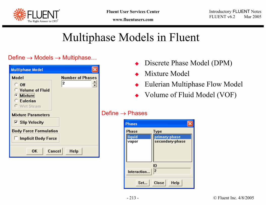
© Fluent Inc. 4/8/2005- 213 -



www.fluentusers.com

Multiphase Models in Fluent

Discrete Phase Model (DPM)Mixture ModelEulerian Multiphase Flow ModelVolume of Fluid Model (VOF)

Define → Models → Multiphase…

Define → Phases

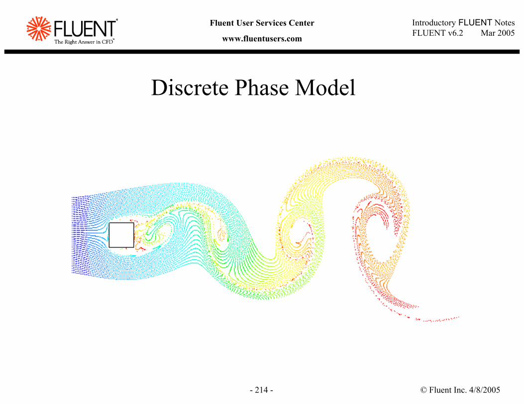
© Fluent Inc. 4/8/2005- 214 -



www.fluentusers.com

Discrete Phase Model

© Fluent Inc. 4/8/2005- 215 -



www.fluentusers.com

Discrete Phase Model (DPM)

Trajectories of particles/droplets/bubbles are computed in a Lagrangian frame.Particles can exchange heat, mass, and momentum with the continuous gas phase.Each trajectory represents a group of particles of the same initial properties.Particle-Particle interaction is neglected.Turbulent dispersion can be modeled with stochastic tracking or a “particle cloud”model.

Numerous sub-modeling capabilities:Heating/cooling of the discrete phaseVaporization and boiling of liquid dropletsVolatile evolution and char combustion for combusting particlesDroplet breakup and coalescence using Spray ModelsErosion/Accretion

© Fluent Inc. 4/8/2005- 216 -



www.fluentusers.com

Applicability of DPM

Flow regime: Bubbly flow, droplet flow, particle-laden flow.Volume loading: Must be Dilute (volume fraction < 12%).Particulate Loading: Low to moderate.Turbulence modeling: Weak to strong coupling between phases.Stokes Number: All ranges of stokes number.

Application examples: Cyclones, spray dryers, particle separation and classification, aerosol dispersion, liquid fuel and coal combustion. etc.

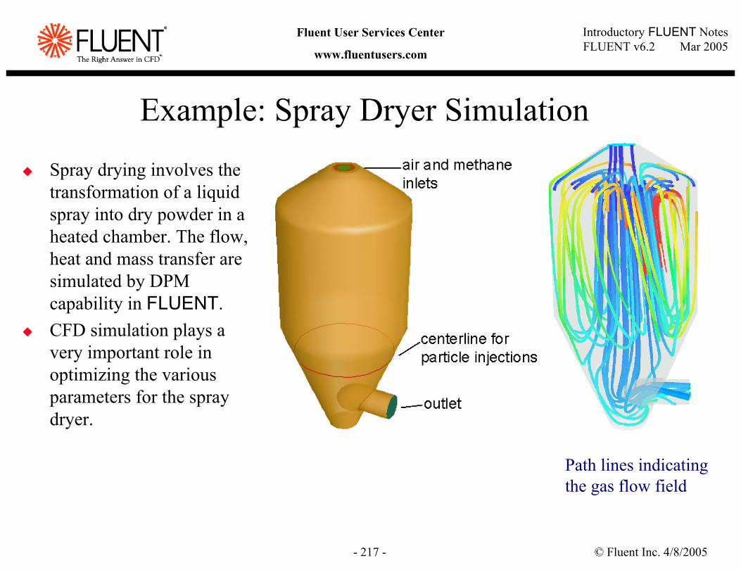
© Fluent Inc. 4/8/2005- 217 -



www.fluentusers.com

Example: Spray Dryer Simulation

Spray drying involves the transformation of a liquid spray into dry powder in a heated chamber. The flow, heat and mass transfer are simulated by DPM capability in FLUENT.CFD simulation plays a very important role in optimizing the various parameters for the spray dryer.

Path lines indicatingthe gas flow field

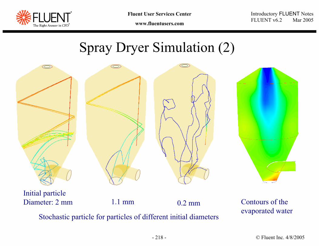
© Fluent Inc. 4/8/2005- 218 -



www.fluentusers.com

Spray Dryer Simulation (2)

Contours of the evaporated water

Stochastic particle for particles of different initial diameters

Initial particleDiameter: 2 mm 1.1 mm 0.2 mm

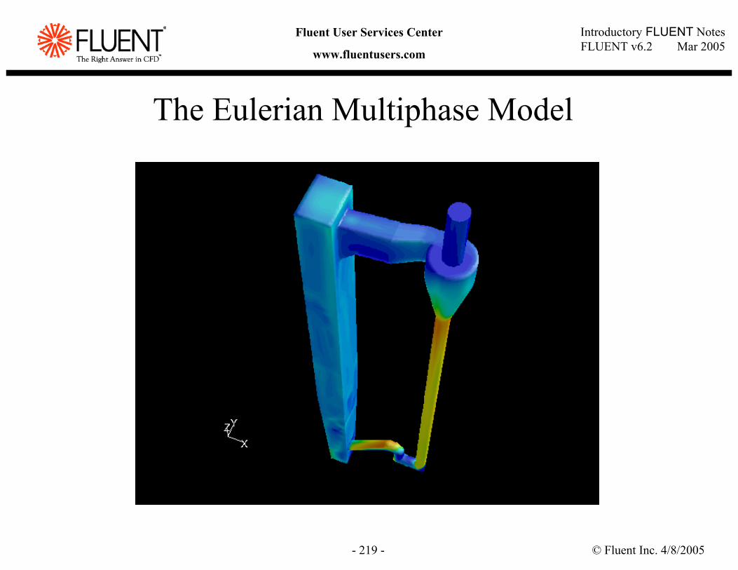
© Fluent Inc. 4/8/2005- 219 -



www.fluentusers.com

The Eulerian Multiphase Model

© Fluent Inc. 4/8/2005- 220 -



www.fluentusers.com

The Eulerian Multiphase ModelDescription

The most sophisticated and general purpose multiphase model.Used to model multiple interpenetrating phases (gas, liquid, and/or solid).

Solves continuity, momentum and energy equations for each phase.Volume fractions characterize equation set for each phase.Coupling among phases achieved through inter-phase exchange terms.

Several models available to define inter-phase exchange coefficients.– Typically drag coefficient models described in terms of local

Reynolds number.Strong coupling makes this model more difficult to use than Mixture Model.

Heat, mass transfer between phases including heterogeneous reactions is possible

Uses a single pressure field for all phases.

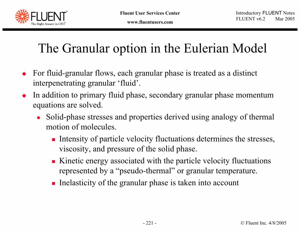
© Fluent Inc. 4/8/2005- 221 -



www.fluentusers.com

The Granular option in the Eulerian Model

For fluid-granular flows, each granular phase is treated as a distinct interpenetrating granular ‘fluid’.In addition to primary fluid phase, secondary granular phase momentum equations are solved.

Solid-phase stresses and properties derived using analogy of thermal motion of molecules.

Intensity of particle velocity fluctuations determines the stresses, viscosity, and pressure of the solid phase.Kinetic energy associated with the particle velocity fluctuations represented by a “pseudo-thermal” or granular temperature.Inelasticity of the granular phase is taken into account

© Fluent Inc. 4/8/2005- 222 -



www.fluentusers.com

Applicability of Eulerian model

Flow regime: Bubbly flow, droplet flow, slurry flow, fluidized beds, particle-laden flow.

Volume loading: Dilute to dense.Particulate Loading: Low to high.Turbulence modeling: Weak to strong coupling between phases.Stokes Number: All ranges of Stokes number.

Application examples: High particle loading flows, slurry flows, sedimentation, hydro-transport, fluidized beds, risers, packed bed reactors.

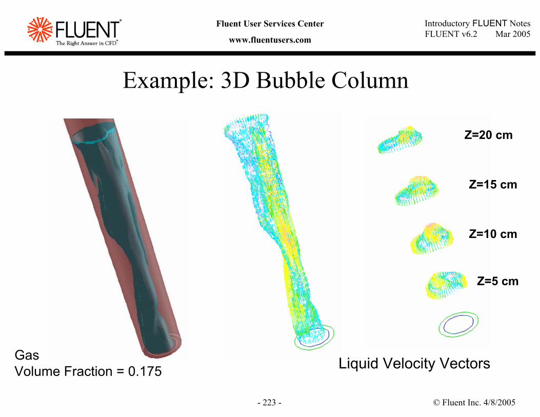
© Fluent Inc. 4/8/2005- 223 -



www.fluentusers.com

Example: 3D Bubble Column

Gas Volume Fraction = 0.175 Liquid Velocity Vectors

Z=5 cm

Z=10 cm

Z=15 cm

Z=20 cm

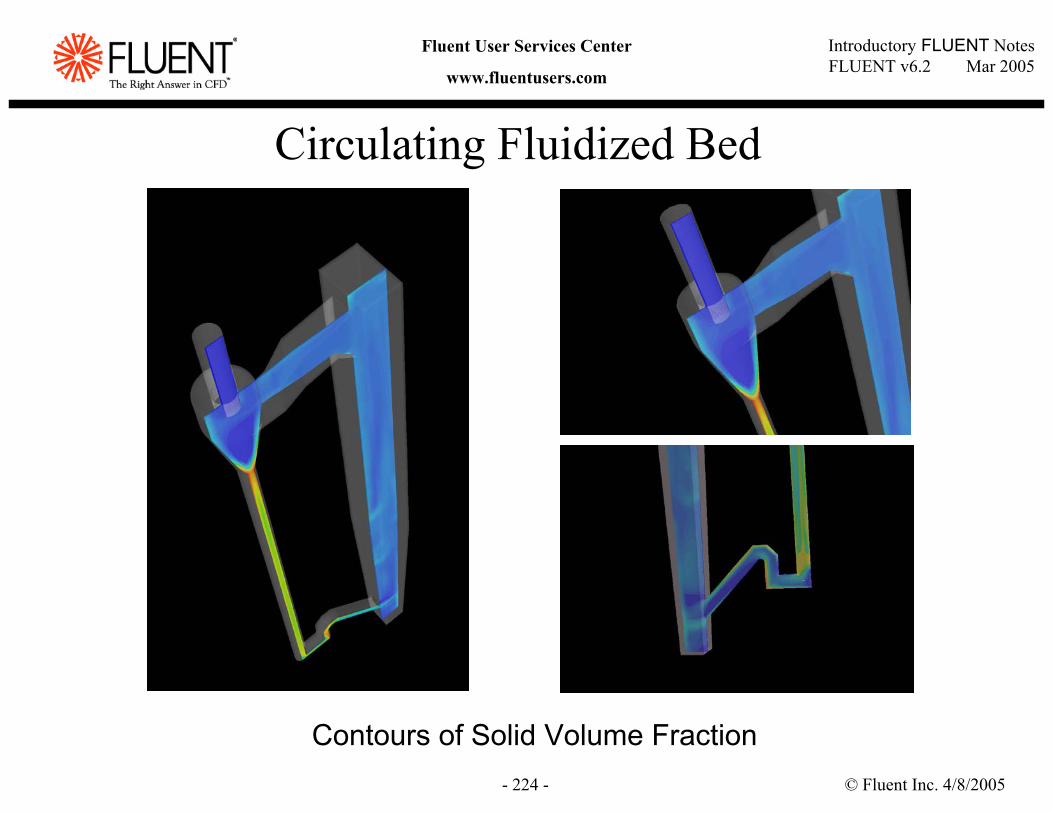
© Fluent Inc. 4/8/2005- 224 -



www.fluentusers.com

Circulating Fluidized Bed

Contours of Solid Volume Fraction

© Fluent Inc. 4/8/2005- 225 -



www.fluentusers.com

Courtesy of Fuller Company

The Mixture Model

© Fluent Inc. 4/8/2005- 226 -



www.fluentusers.com

The Mixture ModelDescription

Mixture model is simplified Eulerian approach for modeling N-phase flows.The simplification is based on main assumption that Stokes number is small, i.e., magnitude and direction of particle velocity vector is close to that of primary fluidSolves the mixture momentum equation (for mass-averaged mixture velocity) and prescribes relative velocities to describe the dispersed phases.

Inter-phase exchange terms depend on relative (slip) velocities which are algebraically determined based on main assumption that St<<1. This means that phase separation can me modeled with Mixture model.Turbulence and Energy equations are also solved for the mixture, if required.Only one of the phases may be defined as compressible.

Solves the transport equation of volume fraction for each secondary phase.Mass exchange is possible including heterogeneous reactionsA submodel for cavitation is available, see the Appendix for more detail.

© Fluent Inc. 4/8/2005- 227 -



www.fluentusers.com

Applicability of Mixture model

Flow regime: Bubbly flow, droplet flow, slurry flow.Volume loading: Dilute to moderately dense.Particulate Loading: Low to moderate.Turbulence modeling: Weak coupling between phases.Stokes Number: Stokes Number < < 1.

Application examples: Hydrocyclones, bubble column reactors, solid suspensions, gas sparging.

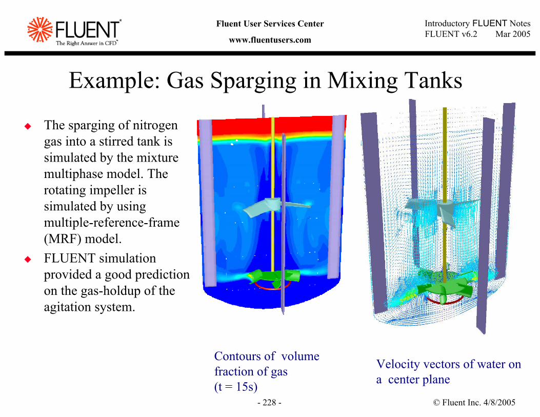
© Fluent Inc. 4/8/2005- 228 -



www.fluentusers.com

Example: Gas Sparging in Mixing Tanks

The sparging of nitrogen gas into a stirred tank is simulated by the mixture multiphase model. The rotating impeller is simulated by using multiple-reference-frame (MRF) model.FLUENT simulation provided a good prediction on the gas-holdup of the agitation system.

Contours of volume fraction of gas (t = 15s)

Velocity vectors of water on a center plane

© Fluent Inc. 4/8/2005- 229 -



www.fluentusers.com

The Volume of Fluid Model (VOF)

© Fluent Inc. 4/8/2005- 230 -



www.fluentusers.com

The Volume of Fluid Model (VOF)Description

The VOF model is designed to track the position of the interfacebetween two or more immiscible fluids.A single momentum equation is solved and the resulting velocity field is shared by all phases.Turbulence and energy equations are also shared by all phases, if required.One of the phases may be defined as compressible.Surface tension and wall adhesion effects can be taken into account.Solves transport equation for volume fraction of each secondary phase. Any phase can be a mixture of species. Heterogeneous reactions are possible.

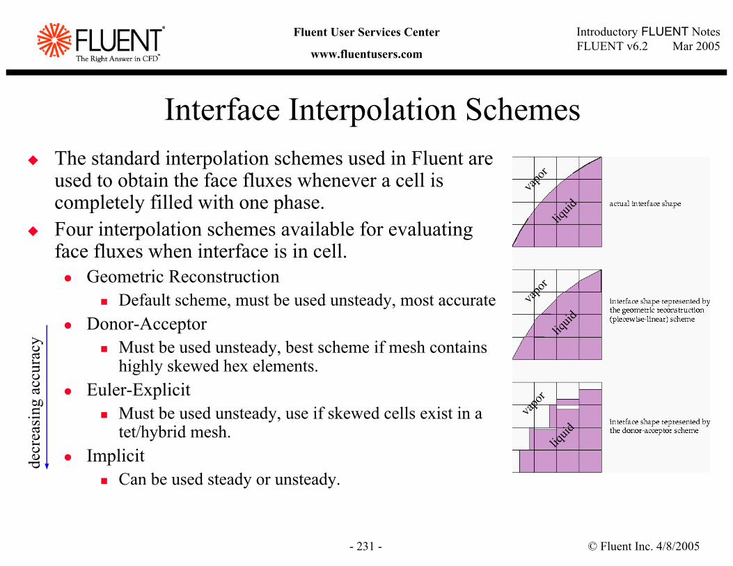
© Fluent Inc. 4/8/2005- 231 -



www.fluentusers.com

Interface Interpolation SchemesThe standard interpolation schemes used in Fluent are used to obtain the face fluxes whenever a cell is completely filled with one phase.Four interpolation schemes available for evaluating face fluxes when interface is in cell.

Geometric ReconstructionDefault scheme, must be used unsteady, most accurate

Donor-AcceptorMust be used unsteady, best scheme if mesh contains highly skewed hex elements.

Euler-ExplicitMust be used unsteady, use if skewed cells exist in a tet/hybrid mesh.

ImplicitCan be used steady or unsteady.

decr

easi

ng a

ccur

acy

vapo

rliq

uid

vapo

rliq

uid

vapo

rliq

uid

© Fluent Inc. 4/8/2005- 232 -



www.fluentusers.com

Applicability of VOF model

Flow regime: Slug flow, stratified/free-surface flow.Volume loading: Dilute to dense.Particulate Loading: Low to high.Turbulence modeling: Weak to moderate coupling between phases.Stokes Number: All ranges of Stokes number.

Application examples:Large slug flows, filling, off-shore oil tank sloshing, boiling, coating.

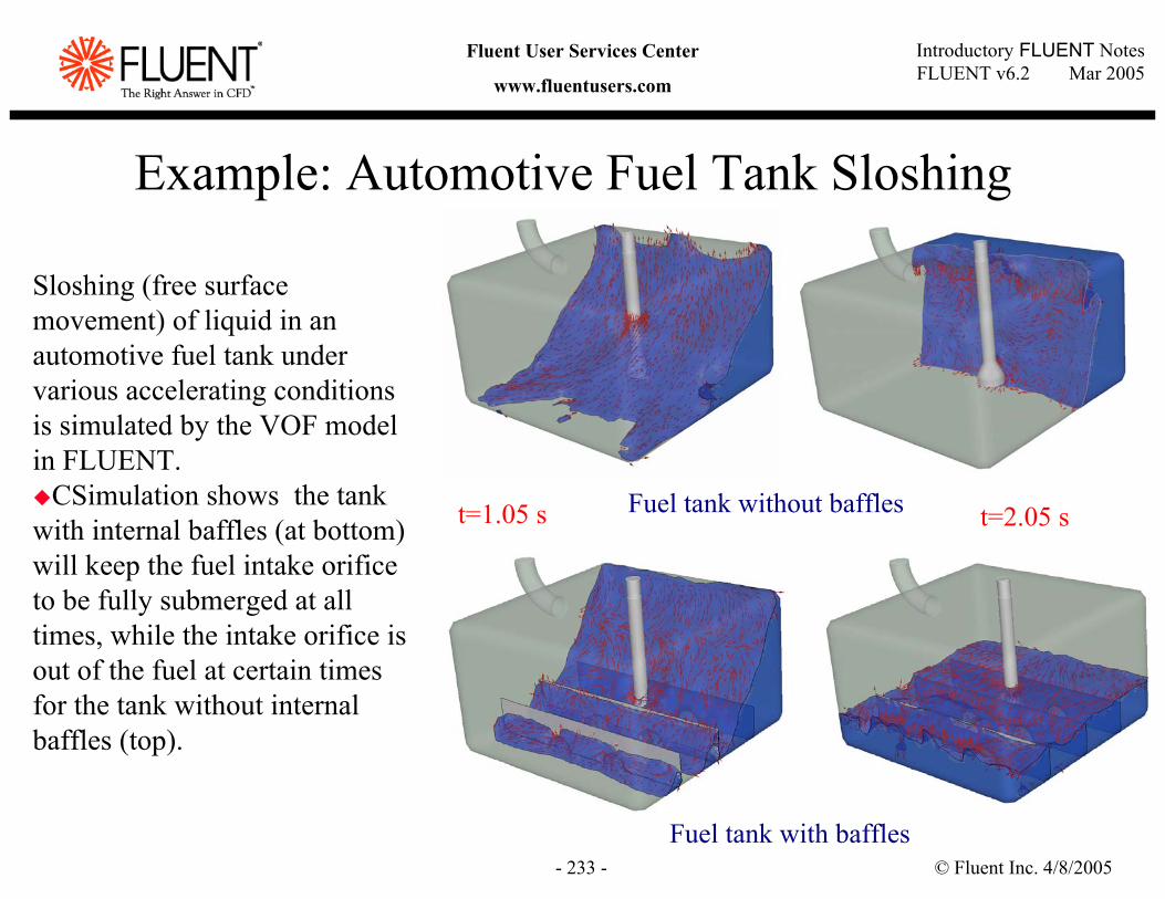
© Fluent Inc. 4/8/2005- 233 -



www.fluentusers.com

Example: Automotive Fuel Tank Sloshing

Fuel tank without baffles

Fuel tank with baffles

Sloshing (free surface movement) of liquid in an automotive fuel tank under various accelerating conditions is simulated by the VOF model in FLUENT.

CSimulation shows the tank with internal baffles (at bottom) will keep the fuel intake orifice to be fully submerged at all times, while the intake orifice is out of the fuel at certain times for the tank without internal baffles (top).

t=1.05 s t=2.05 s

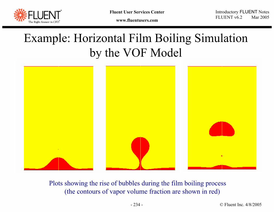
© Fluent Inc. 4/8/2005- 234 -



www.fluentusers.com

Example: Horizontal Film Boiling Simulation by the VOF Model

Plots showing the rise of bubbles during the film boiling process(the contours of vapor volume fraction are shown in red)

© Fluent Inc. 4/8/2005- 235 -



www.fluentusers.com

SummaryChoose an appropriate model for your application based on: Flow regime, volume loading, particulate loading, turbulent or laminar, and Stokes number.

For free surface and stratified flows, choose VOF.For High particle loading flows use Eulerian-Granular Model.For Low-to-Moderate particle loadings consider Stokes number:

For St > 1, Mixture model is not applicable.Choose DPM or Eulerian.

For St ≤ 1, all models are applicableChoose least CPU demanding model based on other requirements.

Strong coupling among phase equations solve better with lowered under-relaxation factors.Users should understand the limitations and applicability of each model.

© Fluent Inc. 4/8/2005- 236 -



www.fluentusers.com

Appendix

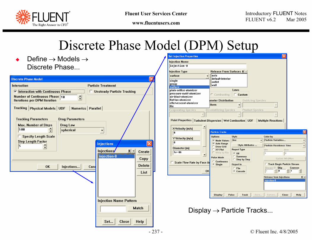
© Fluent Inc. 4/8/2005- 237 -



www.fluentusers.com

Define → Models →Discrete Phase...

Discrete Phase Model (DPM) Setup

Display → Particle Tracks...

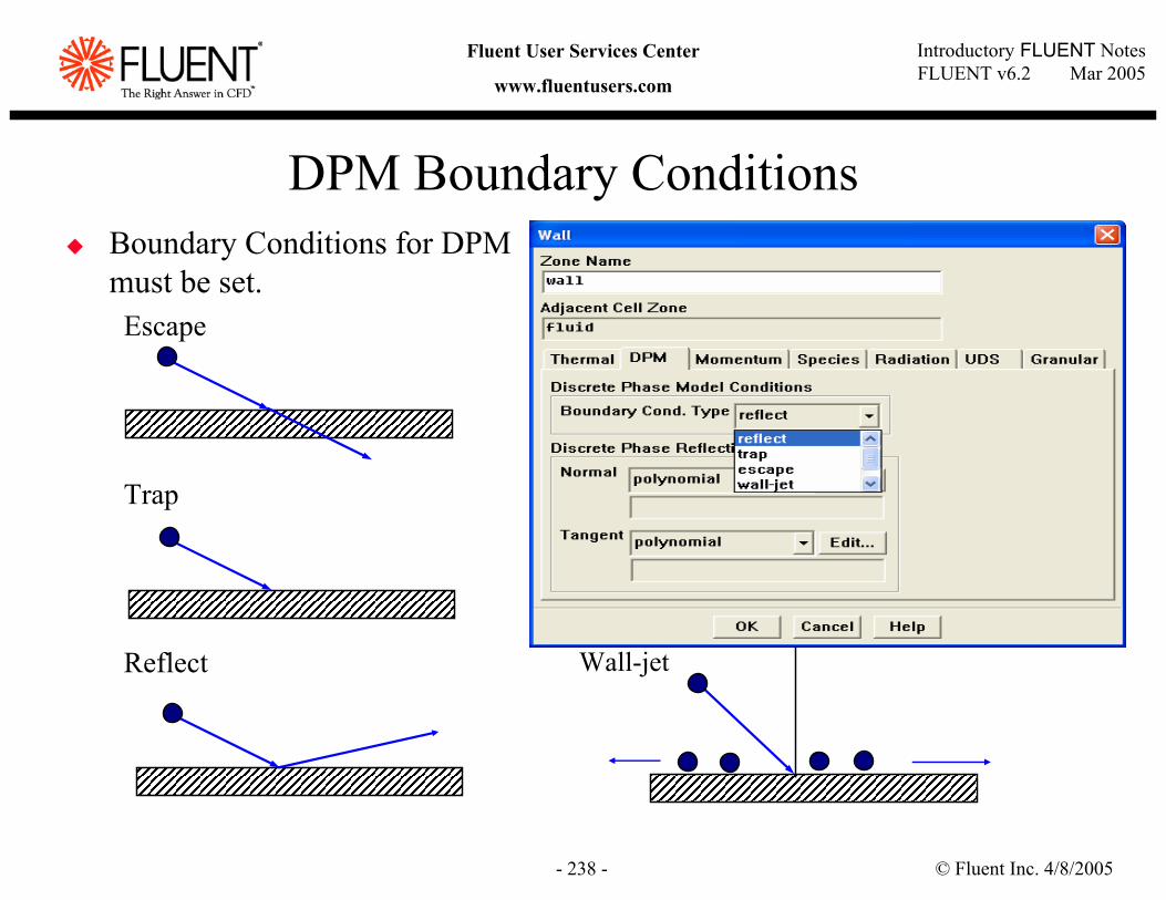
© Fluent Inc. 4/8/2005- 238 -



www.fluentusers.com

DPM Boundary ConditionsBoundary Conditions for DPMmust be set.

Escape

Trap

Reflect Wall-jet

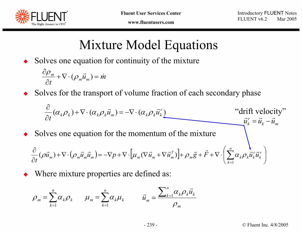
© Fluent Inc. 4/8/2005- 239 -



www.fluentusers.com

Mixture Model EquationsSolves one equation for continuity of the mixture

Solves for the transport of volume fraction of each secondary phase

Solves one equation for the momentum of the mixture

Where mixture properties are defined as:

( ) [ ]

⋅∇+++∇+∇⋅∇+−∇=⋅∇+

∂∂ ∑

=

rk

rkk

n

kkm

Tmmmmmmm uuFguupuuu

trrrrrrrrr ραρµρρ

1)()(

mut mmm &

r=⋅∇+

∂∂ )(ρρ

)()()( rkkkmkkkk uu

trr ραραρα ⋅−∇=⋅∇+

∂∂

∑=

=n

kkkm

1ραρ

m

n

k kkkm

uu

ρρα∑ == 1

rr

mkrk uuu rrr

−=

∑=

=n

kkkm

1µαµ

“drift velocity”

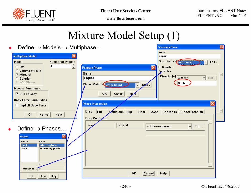
© Fluent Inc. 4/8/2005- 240 -



www.fluentusers.com

Mixture Model Setup (1)Define → Models → Multiphase…

Define → Phases…

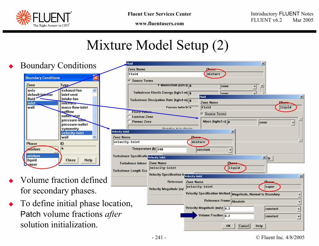
© Fluent Inc. 4/8/2005- 241 -



www.fluentusers.com

Mixture Model Setup (2)Boundary Conditions

Volume fraction defined for secondary phases.To define initial phase location, Patch volume fractions aftersolution initialization.

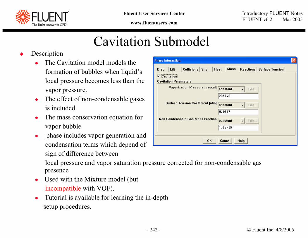
© Fluent Inc. 4/8/2005- 242 -



www.fluentusers.com

Cavitation SubmodelDescription

The Cavitation model models theformation of bubbles when liquid’s local pressure becomes less than thevapor pressure.The effect of non-condensable gasesis included.The mass conservation equation for vapor bubblephase includes vapor generation and condensation terms which depend of sign of difference between local pressure and vapor saturation pressure corrected for non-condensable gas presenceUsed with the Mixture model (but incompatible with VOF).Tutorial is available for learning the in-depth setup procedures.

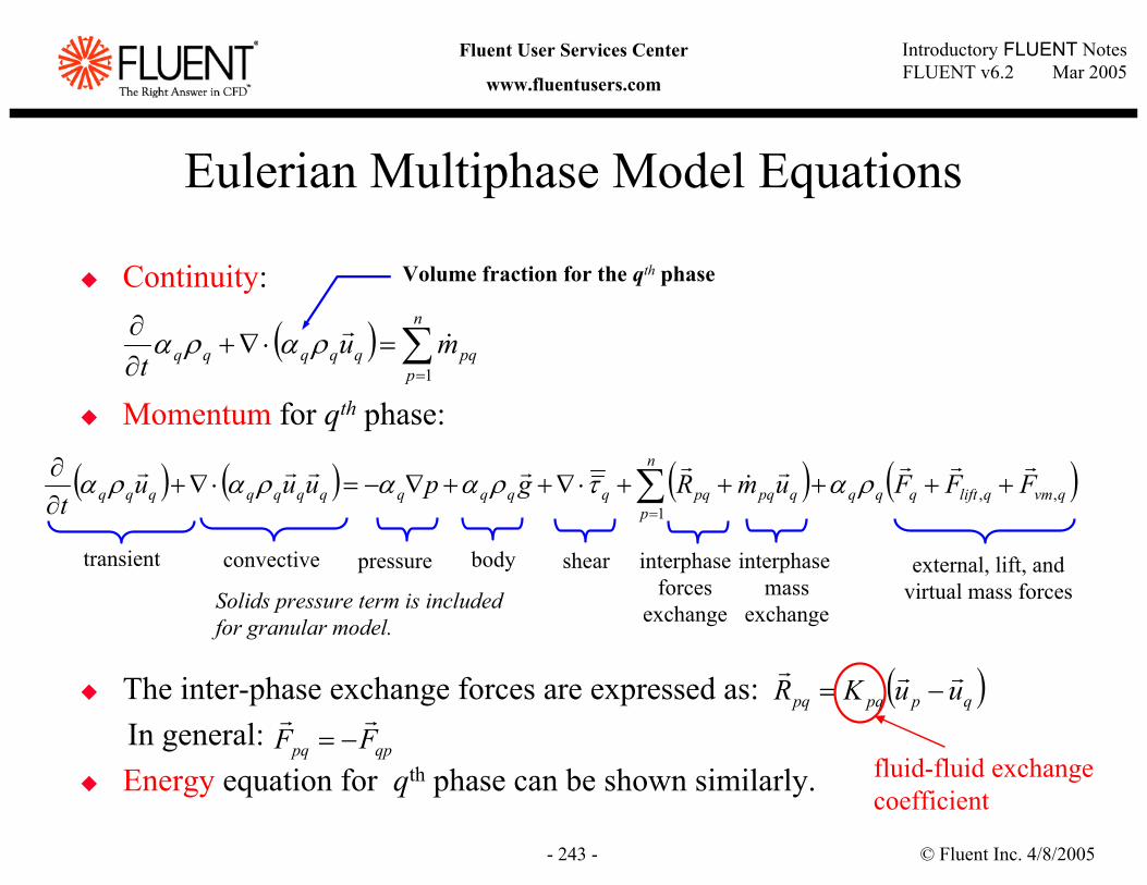
© Fluent Inc. 4/8/2005- 243 -



www.fluentusers.com

Eulerian Multiphase Model Equations

Continuity:

Momentum for qth phase:

The inter-phase exchange forces are expressed as:In general:Energy equation for qth phase can be shown similarly.

( ) ∑=

=⋅∇+∂∂ n

ppqqqqqq mu

t 1

&rραρα

( )qppqpq uuKR rrr−=

qppq FFrr

−=

( ) ( ) ( ) ( )qvmqliftqqq

n

pqpqpqqqqqqqqqqqq FFFumRgpuuu

t ,,1

rrrr&

rrrrr+++++⋅∇++∇−=⋅∇+

∂∂ ∑

=

ρατρααραρα

transient convective pressure shear interphaseforces

exchange

interphasemass

exchange

body external, lift, andvirtual mass forces

Volume fraction for the qth phase

Solids pressure term is included for granular model.

fluid-fluid exchangecoefficient

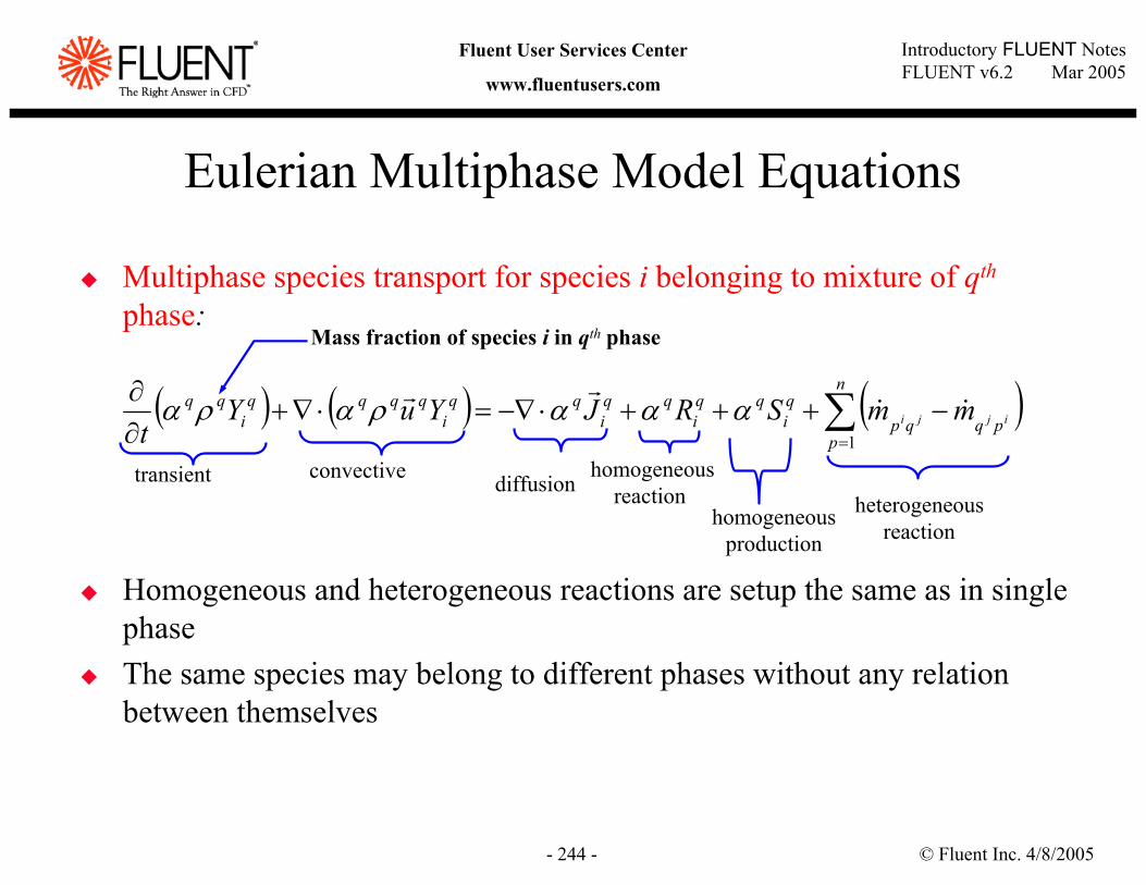
© Fluent Inc. 4/8/2005- 244 -



www.fluentusers.com

Eulerian Multiphase Model Equations

Multiphase species transport for species i belonging to mixture of qth

phase:

Homogeneous and heterogeneous reactions are setup the same as in single phaseThe same species may belong to different phases without any relation between themselves

( ) ( ) ( )∑=

−+++⋅−∇=⋅∇+∂∂ n

ppqqp

qi

qqi

qqi

qqi

qqqqi

qqijji mmSRJYuY

t 1

&&rr αααραρα

transient convective diffusionhomogeneous

reaction homogeneous

production

heterogeneousreaction

Mass fraction of species i in qth phase

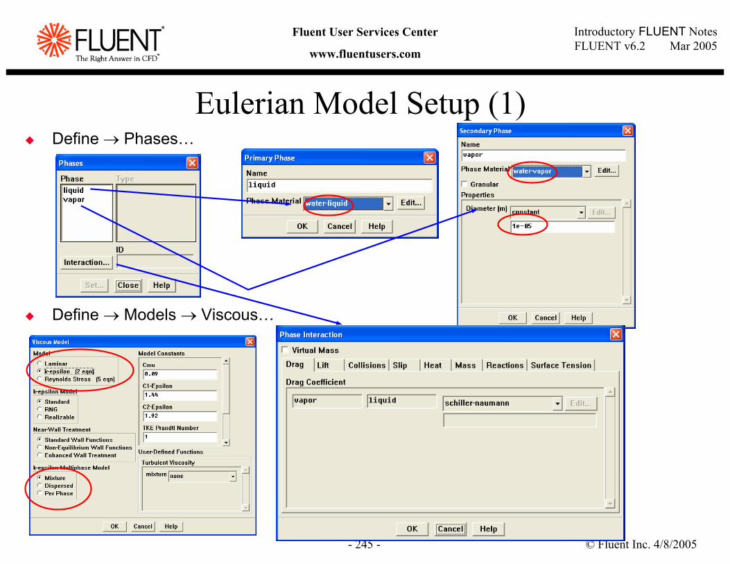
© Fluent Inc. 4/8/2005- 245 -



www.fluentusers.com

Eulerian Model Setup (1)Define → Phases…

Define → Models → Viscous…

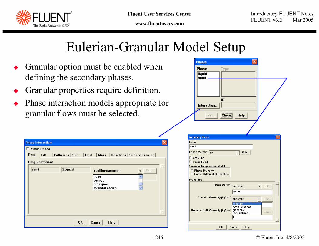
© Fluent Inc. 4/8/2005- 246 -



www.fluentusers.com

Eulerian-Granular Model SetupGranular option must be enabled when defining the secondary phases.Granular properties require definition.Phase interaction models appropriate for granular flows must be selected.

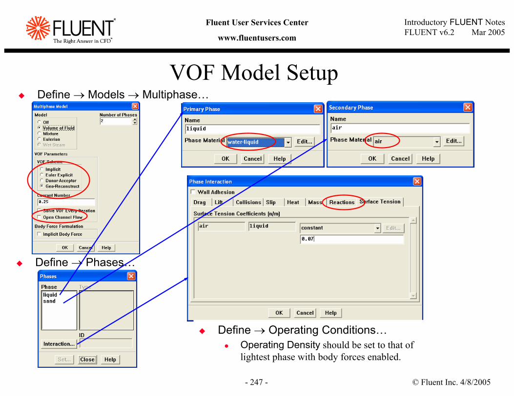
© Fluent Inc. 4/8/2005- 247 -



www.fluentusers.com

VOF Model SetupDefine → Models → Multiphase…


Define → Operating Conditions…Operating Density should be set to that of lightest phase with body forces enabled.

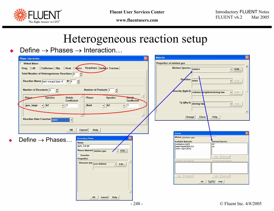
© Fluent Inc. 4/8/2005- 248 -



www.fluentusers.com

Heterogeneous reaction setupDefine → Phases → Interaction…


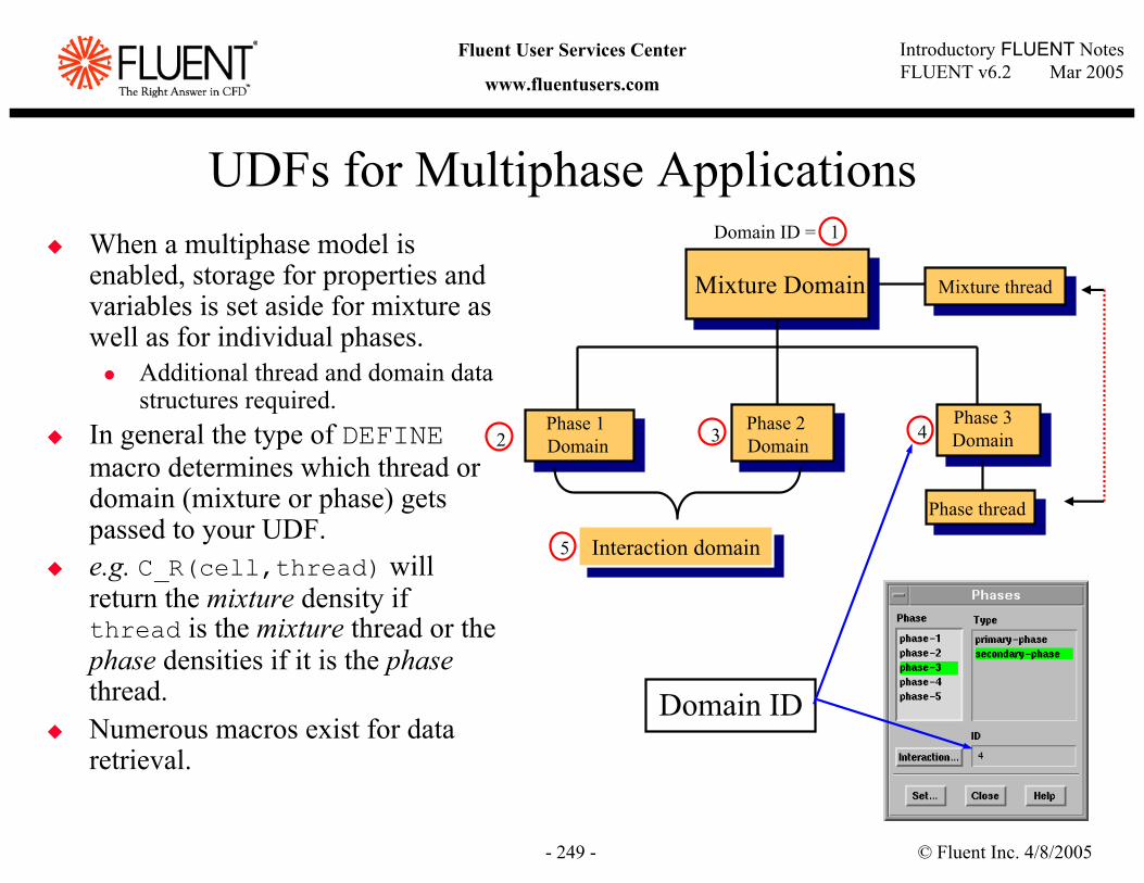
© Fluent Inc. 4/8/2005- 249 -



www.fluentusers.com

UDFs for Multiphase ApplicationsWhen a multiphase model is enabled, storage for properties and variables is set aside for mixture as well as for individual phases.

Additional thread and domain data structures required.

In general the type of DEFINEmacro determines which thread or domain (mixture or phase) gets passed to your UDF.e.g. C_R(cell,thread) will return the mixture density if thread is the mixture thread or the phase densities if it is the phasethread.Numerous macros exist for data retrieval.

Domain ID = 1

Mixture Domain

Phase 1 Domain

Phase 2 Domain

Phase 3Domain2 3 4

Mixture threadMixture thread

Phase thread

Interaction domainInteraction domain5

Domain ID

© Fluent Inc. 4/8/2005- 250 -



www.fluentusers.com

Reacting-Flow Models in FLUENT

© Fluent Inc. 4/8/2005- 251 -



www.fluentusers.com

Outline

Aspects of Reaction Modeling and Fundamental ConceptsReaction Models in FLUENT

OverviewFast Chemistry Models: eddy dissipation, premixed, partially premixed, non-premixedModerately non-equilibrium model: Laminar flamelet for non-premixed flamesFinite-rate Chemistry Models: Laminar finite-rate, eddy dissipation concept (EDC), composition PDF

ISAT Algorithm, DPM and Pollutant Formation ModelsSurface ReactionsExamples and Case Studies

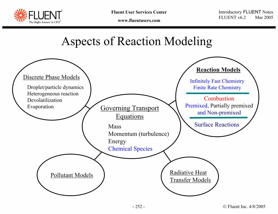
© Fluent Inc. 4/8/2005- 252 -



www.fluentusers.com

Aspects of Reaction Modeling

Discrete Phase ModelsDroplet/particle dynamicsHeterogeneous reactionDevolatilizationEvaporation Governing Transport

EquationsMassMomentum (turbulence)EnergyChemical Species

Reaction Models

CombustionPremixed, Partially premixed

and Non-premixed

Pollutant Models Radiative Heat Transfer Models

Infinitely Fast ChemistryFinite Rate Chemistry

Surface Reactions

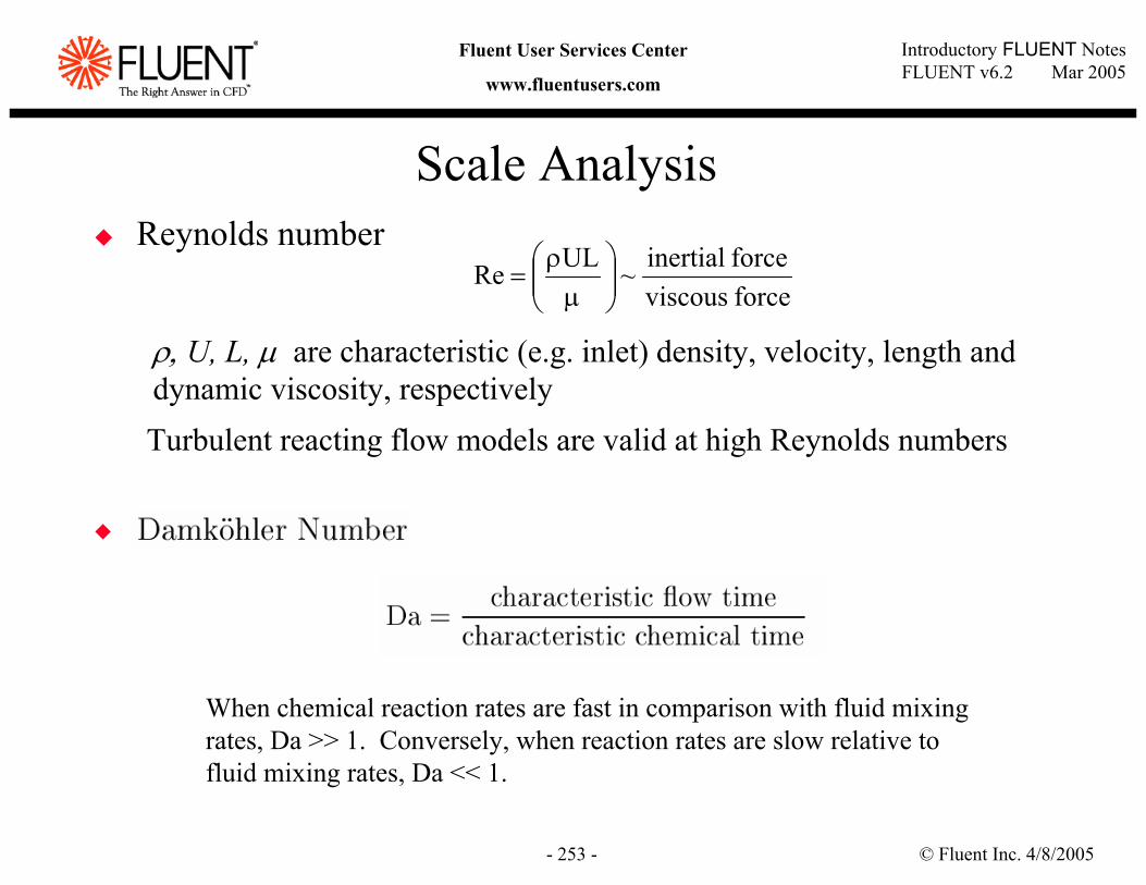
© Fluent Inc. 4/8/2005- 253 -



www.fluentusers.com

Scale Analysis

forceviscousforceinertial~ULRe

µ

ρ=

ρ, U, L, µ are characteristic (e.g. inlet) density, velocity, length anddynamic viscosity, respectivelyTurbulent reacting flow models are valid at high Reynolds numbers

Reynolds number

When chemical reaction rates are fast in comparison with fluid mixingrates, Da >> 1. Conversely, when reaction rates are slow relative tofluid mixing rates, Da << 1.

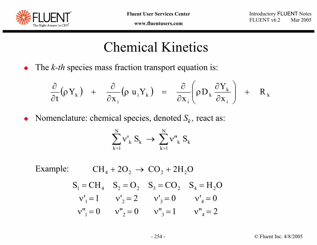
© Fluent Inc. 4/8/2005- 254 -



www.fluentusers.com

Chemical KineticsThe k-th species mass fraction transport equation is:

Nomenclature: chemical species, denoted Sk , react as:

Example:

( ) ( ) ki

kk

iki

ik R

xYD

xYu

xY

t+

∂∂

ρ∂∂

=ρ∂∂

+ρ∂∂

∑∑==

ν→νN

1kkk

N

1kkk S"S'

OH2COO2CH 2224 +→+

2"1"0"0"0'0'2'1'OHSCOSOSCHS

4321

4321

24232241

=ν=ν=ν=ν=ν=ν=ν=ν

====

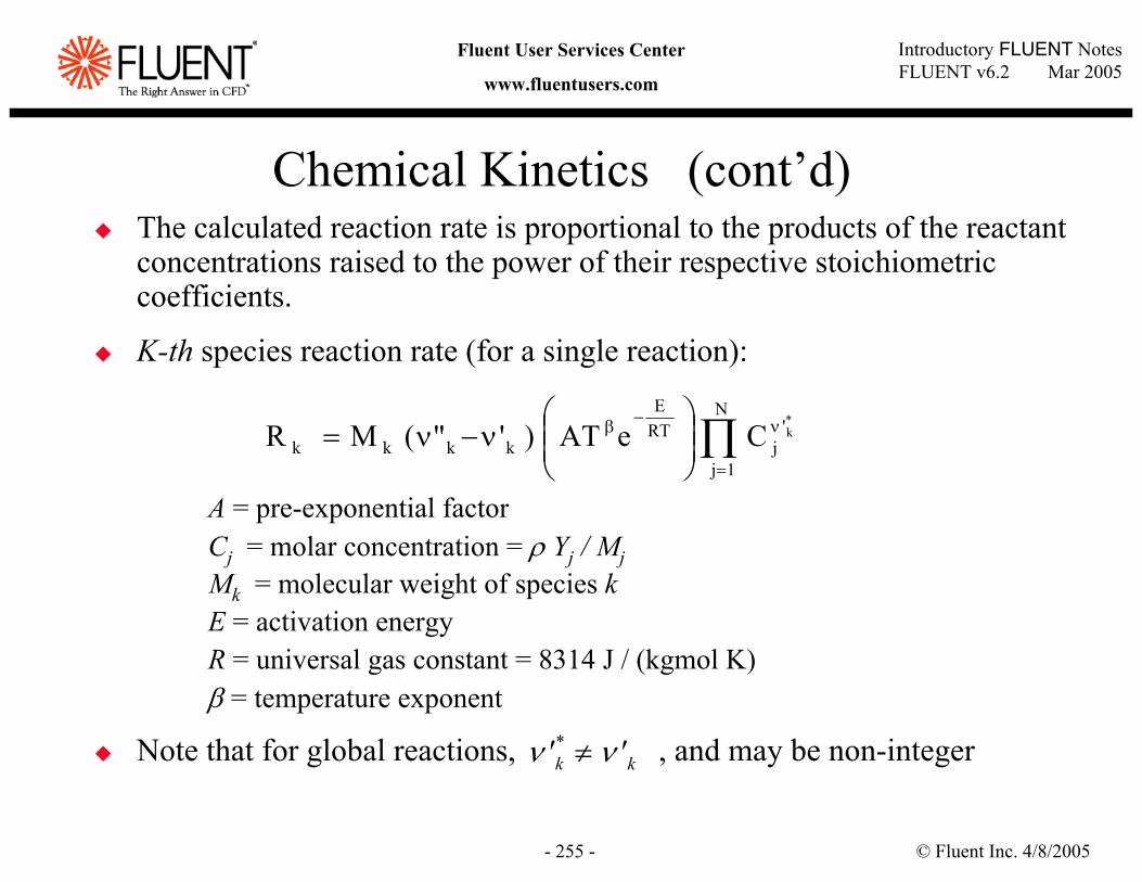
© Fluent Inc. 4/8/2005- 255 -



www.fluentusers.com

Chemical Kinetics (cont’d)The calculated reaction rate is proportional to the products of the reactant concentrations raised to the power of their respective stoichiometric coefficients.

K-th species reaction rate (for a single reaction):

A = pre-exponential factorCj = molar concentration = ρ Yj / MjMk = molecular weight of species kE = activation energyR = universal gas constant = 8314 J / (kgmol K)β = temperature exponent

Note that for global reactions, , and may be non-integer

∏=

ν−β

ν−ν=

N

1j

'j

RTE

kkkk

*kCeAT)'"(MR

k*k '' νν ≠

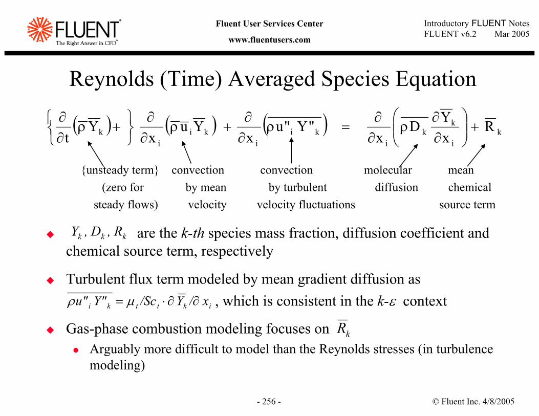
© Fluent Inc. 4/8/2005- 256 -



www.fluentusers.com

Reynolds (Time) Averaged Species Equation

unsteady term convection convection molecular mean(zero for by mean by turbulent diffusion chemical

steady flows) velocity velocity fluctuations source term

are the k-th species mass fraction, diffusion coefficient and chemical source term, respectively

Turbulent flux term modeled by mean gradient diffusion as, which is consistent in the k-ε context

Gas-phase combustion modeling focuses on Arguably more difficult to model than the Reynolds stresses (in turbulence modeling)

( ) ( ) ( ) ki

kk

iki

iki

ik R

xYD

x"Y"u

xYu

xY

t+

∂∂

ρ∂∂

=ρ∂∂

+ρ∂∂

+ρ

∂∂

kkk R,D,Y

kRikttki x/Y/ScY"u" ∂∂⋅= µρ

© Fluent Inc. 4/8/2005- 257 -



www.fluentusers.com

Difficulties of Modeling Reactive FlowsSolving directly the species transport and the Arrhenius rate equations for a reacting flow problem is difficult and impractical:

TurbulenceMost industrial flows are turbulent.DNS of non-reacting and reacting turbulent flows is not possible because ofthe wide range of time and length scales.

ChemistryRealistic chemical mechanisms cannot be described by a single reaction equation.

Tens of species, hundreds of reactionsKnown in detail for only a limited number of fuels

Stiff kinetics (wide range of reacting time scales)Turbulence-Chemistry Interaction

The sensitivity of reaction rates to local changes is complicated by enhanced mixing of turbulent flows.

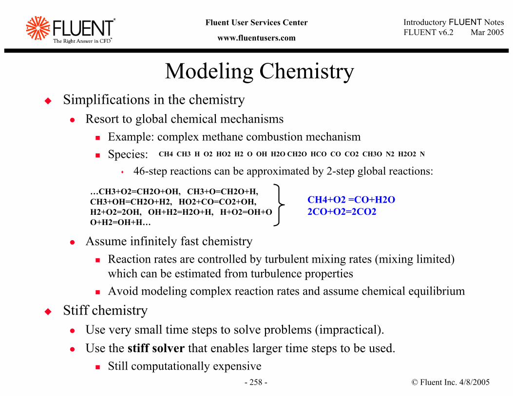
© Fluent Inc. 4/8/2005- 258 -



www.fluentusers.com

Modeling ChemistrySimplifications in the chemistry

Resort to global chemical mechanismsExample: complex methane combustion mechanismSpecies:

46-step reactions can be approximated by 2-step global reactions:

Assume infinitely fast chemistryReaction rates are controlled by turbulent mixing rates (mixing limited) which can be estimated from turbulence propertiesAvoid modeling complex reaction rates and assume chemical equilibrium

Stiff chemistryUse very small time steps to solve problems (impractical).Use the stiff solver that enables larger time steps to be used.

Still computationally expensive

CH4 CH3 H O2 HO2 H2 O OH H2O CH2O HCO CO CO2 CH3O N2 H2O2 N

…CH3+O2=CH2O+OH, CH3+O=CH2O+H, CH3+OH=CH2O+H2, HO2+CO=CO2+OH,H2+O2=2OH, OH+H2=H2O+H, H+O2=OH+OO+H2=OH+H…

CH4+O2 =CO+H2O2CO+O2=2CO2

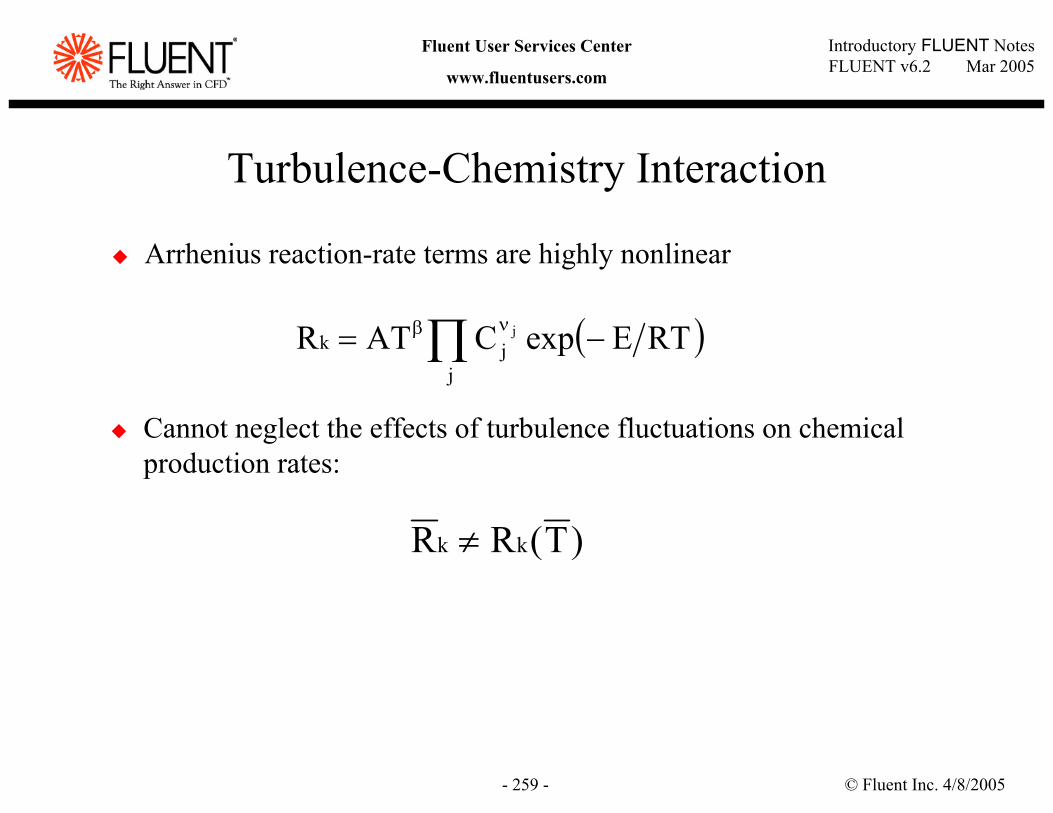
© Fluent Inc. 4/8/2005- 259 -



www.fluentusers.com

Turbulence-Chemistry Interaction

( )RTEexpCATRj

jkj −= ∏ νβ

Arrhenius reaction-rate terms are highly nonlinear

Cannot neglect the effects of turbulence fluctuations on chemical production rates:

)T(RR kk ≠

© Fluent Inc. 4/8/2005- 260 -



www.fluentusers.com

Gas-Phase Reacting Flows: ConfigurationsNon-Premixed combustion

Fuel and oxidizer enter the reaction zone in separate streamsCan be simplified to a mixing problem (under certain restrictions)Turbulent eddies distort the laminar flame shape and enhance mixingExamples: pulverized coal furnaces, diesel engine, pool fires, …

Premixed combustionFuel and oxidizer are already mixed at the molecular level prior to ignition, a very thin flame front propagates into the unburnt regionsRate of propagation (the laminar flame speed) depends on the internal flame structure and turbulence eddies, hence it is much more difficult to model than the non-premixed combustionExamples: lean-premixed gas turbine combustors, internal combustion engines, …

Partially premixed combustionReacting systems with both non-premixed and premixed fuel/oxidizer streamsExample: lean premixed combustors with diffusion pilot flames and/or cooling air jets, …

© Fluent Inc. 4/8/2005- 261 -



www.fluentusers.com

Outline




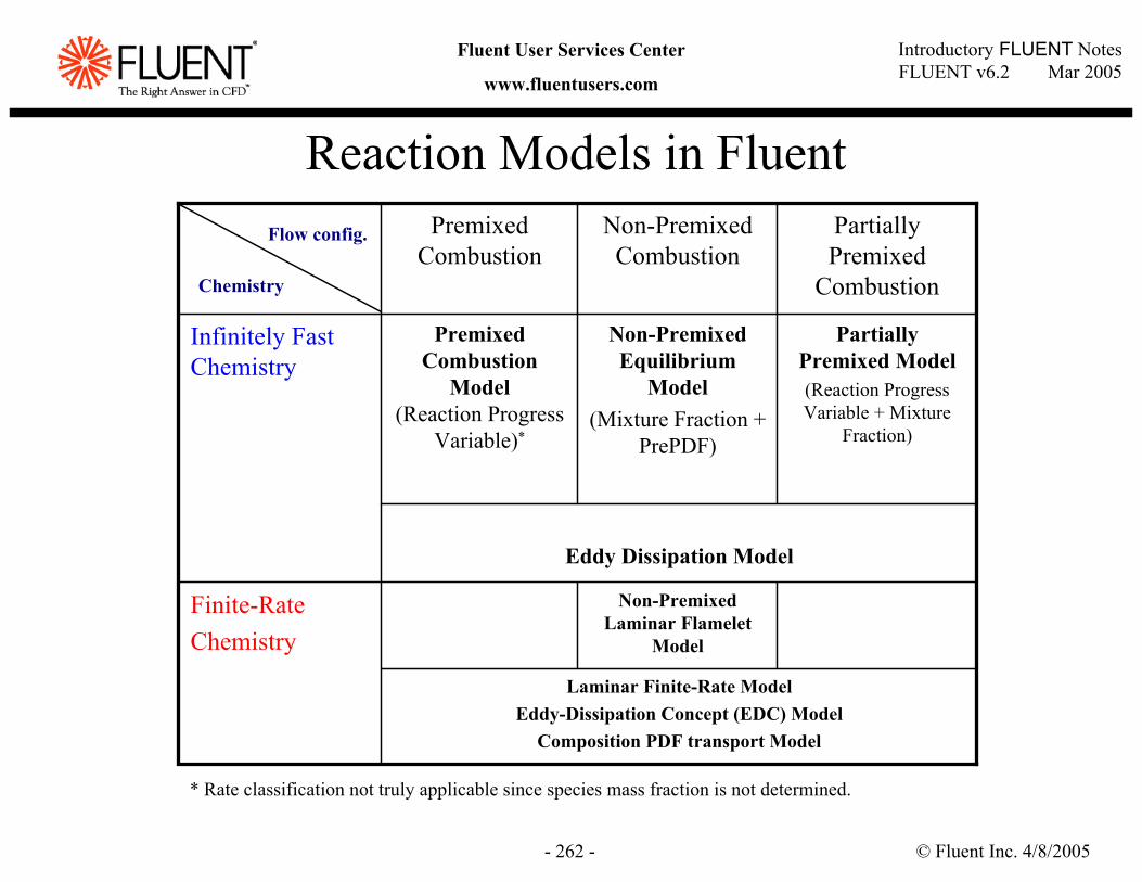
© Fluent Inc. 4/8/2005- 262 -



www.fluentusers.com

Reaction Models in Fluent

Laminar Finite-Rate ModelEddy-Dissipation Concept (EDC) Model

Composition PDF transport Model

Non-Premixed Laminar Flamelet

Model

Finite-RateChemistry

Eddy Dissipation Model

Partially Premixed Model(Reaction Progress Variable + Mixture

Fraction)

Non-Premixed Equilibrium

Model(Mixture Fraction +

PrePDF)

Premixed Combustion

Model(Reaction Progress

Variable)*

Infinitely Fast Chemistry

Partially Premixed

Combustion

Non-Premixed Combustion

Premixed Combustion

* Rate classification not truly applicable since species mass fraction is not determined.

Flow config.

Chemistry

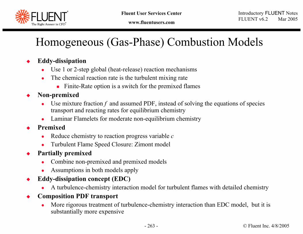
© Fluent Inc. 4/8/2005- 263 -



www.fluentusers.com

Homogeneous (Gas-Phase) Combustion ModelsEddy-dissipation

Use 1 or 2-step global (heat-release) reaction mechanismsThe chemical reaction rate is the turbulent mixing rate

Finite-Rate option is a switch for the premixed flamesNon-premixed

Use mixture fraction f and assumed PDF, instead of solving the equations of species transport and reacting rates for equilibrium chemistryLaminar Flamelets for moderate non-equilibrium chemistry

PremixedReduce chemistry to reaction progress variable cTurbulent Flame Speed Closure: Zimont model

Partially premixedCombine non-premixed and premixed modelsAssumptions in both models apply

Eddy-dissipation concept (EDC)A turbulence-chemistry interaction model for turbulent flames with detailed chemistry

Composition PDF transportMore rigorous treatment of turbulence-chemistry interaction than EDC model, but it is substantially more expensive

© Fluent Inc. 4/8/2005- 264 -



www.fluentusers.com

Outline




© Fluent Inc. 4/8/2005- 265 -



www.fluentusers.com

Eddy Dissipation Model (EDM)

A model for estimating the mean reaction rate (of species k), Rk

Reaction rate is defined using the eddy-breakup model:Assumes that chemical reactions occur much faster than turbulence can mix reactants into the flame ( Da >> 1)Combustion is completely controlled by turbulent mixing rates which are proportional to the large-eddy lifetime scale, k /ε

Chemical reaction is approximated by the global (1 or 2 step) mechanismReynolds (time) averaged species mass fraction equations for (N-1) species are solved Finite-Rate/Eddy Dissipation Option: the smaller of the Arrhenius and eddy-dissipation rates is used as the reaction rate

© Fluent Inc. 4/8/2005- 266 -



www.fluentusers.com

Eddy Dissipation Model (cont’d)Applicability:Flow Regime: Turbulent flow (high Re)Chemistry: Fast Chemistry (Da >> 1)Flow configuration : Premixed, non-premixed, partially premixed

ApplicationsWidely used for chemical reacting flows at high Da and ReExample: BERL combustor, IFRF coal combustion

LimitationsUnreliable when flow (mixing) and kinetic time scales are comparable (Da ~1)

Does not predict kinetically-controlled intermediate species and dissociation effects

Cannot realistically model phenomena which depend on detailed kinetics such as ignition, extinction and low-Da flows

© Fluent Inc. 4/8/2005- 267 -



www.fluentusers.com

Premixed Combustion ModelIn premixed system combustion within the domain occurs as a thin flame front that propagates into the unburnt region of reactants

Flame front propagates at a speed dictated by laminar flame speed and local turbulence eddiesA reaction progress variable c is solved to predict the position of the flame front (Zimont model)

c is defined such that c = 0 for unburnt mixture and c = 1 for burnt mixture.For non-adiabatic flows, temperature is determined from local enthalpy which is calculated from enthalpy transport equation.

Applicability:Flow regime: turbulentChemistry: infinitely fast chemistry

ApplicationLean-premixed gas turbine combustor

© Fluent Inc. 4/8/2005- 268 -



www.fluentusers.com

Partially Premixed Combustion ModelReaction progress variable and mixture fraction approach are combined

Solves transport equations for reaction progress variable c, mixture fraction f , and its variance.The premixed reaction-progress variable, c, determines the position of the flame front.

Behind the flame front (c = 1), the mixture is burnt and the equilibrium or laminar flamelet mixture fraction solution is used.Ahead of the flame front (c = 0), the species mass fractions, temperature, and density are calculated from the mixed but unburnt mixture fraction.Within the flame (0 < c <1), a linear combination of the unburnt and burnt mixtures is used.

Applicability of the Premixed combustion modelFlow regime: turbulentChemistry: Equilibrium or moderate non-equilibrium (Flamelet)Flow configuration : partially premixed

ApplicationSystems with both premixed and non-premixed streams

© Fluent Inc. 4/8/2005- 269 -



www.fluentusers.com

Non-Premixed Equilibrium ModelFor infinitely fast chemistry in turbulent flows, reaction proceeds to chemical equilibrium instantaneously when the fuel and oxidizer mix (mixing limited).The species and enthalpy transport equations collapse into a single conservation equation for mixture fraction f , under the following assumptions

Species diffusion coefficients are equalLewis number (Le) = 1Moderate Mach number

Mixture fraction can be directly related to species mass fraction, mixture density, and mixture temperature

These relations are known for instantaneous (not time-averaged) dataA probability density function (PDF) is used to relate instantaneous data to time-averaged data (turbulent reacting flow simulations predict time-averaged properties)

PDF is assumed to be a beta function (which can describe a wide range of PDF shapes)Requires the variance of f which is based on local turbulence parameters

© Fluent Inc. 4/8/2005- 270 -



www.fluentusers.com

Non-Premixed Equilibrium Model (cont’d)Transport equations for mixture fraction and mixture fraction variance are solved (instead of the individual species equations), reaction is simplified as a mixing problemApplicability:

Flow regime: Turbulent flowChemistry: Fast chemistry (assuming equilibrium condition)Flow configuration: Non-premixedApplications

Model of choice if assumptions (see the previous slide) are valid for gas-phase combustion problemsAccurate tracking of intermediate species concentrations and dissociation effects without requiring the knowledge of detailed chemical kinetic rates

Turbulence-chemistry interactions are accounted for rigorously via PDFsLimitations

Unreliable when mixing and kinetic time scales are comparable (Da ~1)

Cannot realistically model phenomena which depend on detailed kinetics such as ignition, extinction and low-Da flows

© Fluent Inc. 4/8/2005- 271 -



www.fluentusers.com

Outline




© Fluent Inc. 4/8/2005- 272 -



www.fluentusers.com

Laminar Flamelet Model For Non-premixed Flames

Extension of mixture fraction/PDF model to problems in where moderate chemical non-equilibrium effects are importantTurbulent diffusion flame is modeled as an ensemble of stretched laminar flamlets(opposed flow diffusion flames)

Temperature, density and species (for adiabatic) specified by two parameters, the mixture fraction and scalar dissipation rate χ (flame strain rate).

Applicability: Flow regime: Turbulent flowChemistry: Moderate non-equilibrium due to aerodynamic straining, not suitable

for slow chemistryFlow configuration: Non-premixedApplications

Predictions of lift-off and blow-off phenomena in jet flames

© Fluent Inc. 4/8/2005- 273 -



www.fluentusers.com

Outline




© Fluent Inc. 4/8/2005- 274 -



www.fluentusers.com

Detailed Chemistry ModelsFor reactions described by detailed kinetic mechanisms, the chemistry models are numerically stiff : tens of species, hundreds of reactions with large spread in reaction time scalesCHEMKIN-format reaction mechanisms and thermal properties can be imported directlyAvailable Models:

Laminar finite rateEDC ModelPDF transportKINetics model

Detailed kinetics are used to model:Flame ignition and extinctionPollutants (NOx, CO, UHCs)Slow (non-equilibrium) chemistry

CPU intensive, ISAT (In-situ Adaptive Tabulation) algorithm can be used for acceleration (Laminar, EDC, PDF transport models)

© Fluent Inc. 4/8/2005- 275 -



www.fluentusers.com

Laminar Finite-Rate ModelStiff chemistry solver (available for both coupled and segregated solver)Applicability of the finite-rate model

Flow regime: Laminar flowChemistry: Finite-rate chemistryFlow configuration : Premixed, non-premixed, partially premixed

DeficienciesCPU intensive: ISAT (In-situ Adaptive Tabulation) algorithm for accelerationUnsuitable for turbulent combustion problems

ApplicationsLaminar diffusion flame, laminar premixed flames in gas furnaces, etc.

© Fluent Inc. 4/8/2005- 276 -



www.fluentusers.com

Eddy Dissipation Concept (EDC) ModelEDC model is an extension of the eddy-dissipation model to account for finite-rate chemistry and detailed mechanisms in turbulent flows.EDC is a turbulence-chemistry interaction model and species transport equation is solved for each speciesApplicability of the EDC model

Flow Regime: Turbulent flowChemistry: Finite-rate chemistry Flow configuration : Premixed, non-premixed, partially premixed

DeficienciesCPU intensive. ISAT (In-situ Adaptive Tabulation) algorithm can be used for acceleration

ApplicationsPredictions of finite-rate phenomena in turbulent reacting flows, for example, slow CO burnout or nitrogen oxides formation

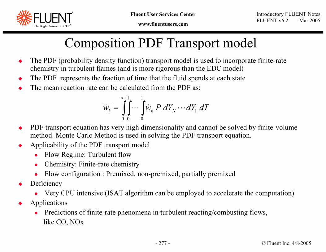
© Fluent Inc. 4/8/2005- 277 -



www.fluentusers.com

Composition PDF Transport modelThe PDF (probability density function) transport model is used to incorporate finite-rate chemistry in turbulent flames (and is more rigorous than the EDC model)The PDF represents the fraction of time that the fluid spends at each stateThe mean reaction rate can be calculated from the PDF as:

PDF transport equation has very high dimensionality and cannot be solved by finite-volume method. Monte Carlo Method is used in solving the PDF transport equation. Applicability of the PDF transport model

Flow Regime: Turbulent flowChemistry: Finite-rate chemistryFlow configuration : Premixed, non-premixed, partially premixed

DeficiencyVery CPU intensive (ISAT algorithm can be employed to accelerate the computation)

ApplicationsPredictions of finite-rate phenomena in turbulent reacting/combusting flows,like CO, NOx

dTdYdYPww Nkk 10

1

0

1

0

L&L& ∫ ∫ ∫∞

=

© Fluent Inc. 4/8/2005- 278 -



www.fluentusers.com

Outline




© Fluent Inc. 4/8/2005- 279 -



www.fluentusers.com

In-Situ Adaptive Tabulation (ISAT) AlgorithmMotivations

In EDC, Composition PDF, and laminar finite rate models, the stiff reaction system (a set of ODE’s) is solved for each cell (or for each particle) in every iteration. Table look-up method is effective, but the traditional prior tabulation approach is not feasible for a system with a large number of species; moreover, it is inefficient since only a small part of the composition space is accessed during a simulation.

In-Situ Adaptive TabulationTable is constructed in situ - as the reactive flow calculation is performed, so that only the accessed region of the composition space is tabulated. Tabulation error is controlled adaptively by the user specified tolerance.

AdvantageAvoid the repeating work in numerical integration, and reduce cpu time significantly.

Initial iterations are slower as table is being built, but accelerate as more retrieval operations take place.

ApplicationISAT can be used with PDF-transport, EDC, and laminar finite-rate models

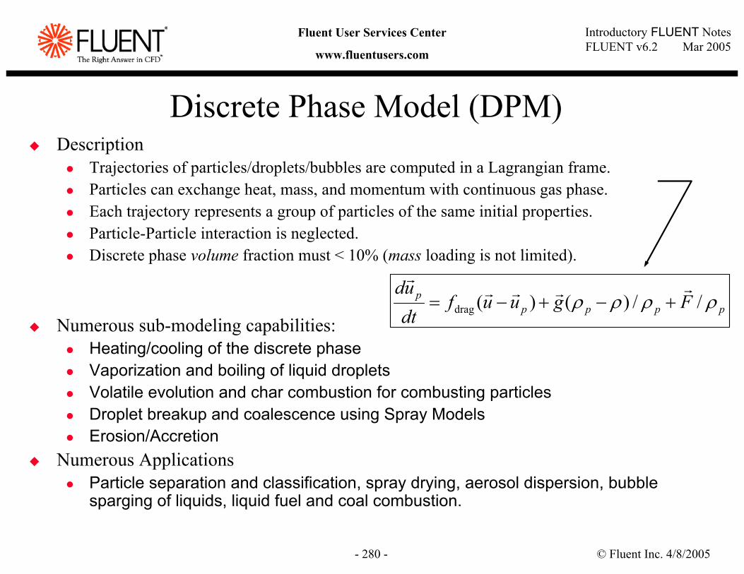
© Fluent Inc. 4/8/2005- 280 -



www.fluentusers.com

Discrete Phase Model (DPM)Description

Trajectories of particles/droplets/bubbles are computed in a Lagrangian frame.Particles can exchange heat, mass, and momentum with continuous gas phase.Each trajectory represents a group of particles of the same initial properties.Particle-Particle interaction is neglected.Discrete phase volume fraction must < 10% (mass loading is not limited).

Numerous sub-modeling capabilities:Heating/cooling of the discrete phaseVaporization and boiling of liquid dropletsVolatile evolution and char combustion for combusting particlesDroplet breakup and coalescence using Spray ModelsErosion/Accretion

Numerous ApplicationsParticle separation and classification, spray drying, aerosol dispersion, bubble sparging of liquids, liquid fuel and coal combustion.

ppppp Fguuf

dtud

ρρρρ //)()(drag

rrrrr

+−+−=

© Fluent Inc. 4/8/2005- 281 -



www.fluentusers.com

NOx ModelsNOx consists of mostly nitric oxide (NO) which is harmful to the environment.

Three mechanisms included in FLUENT for NOx production:Thermal NOx - Zeldovich mechanism (oxidation of atmospheric N)

Most significant at high temperaturesPrompt NOx - empirical mechanisms by De Soete, Williams, etc.

Contribution is in general smallSignificant at fuel rich zones

Fuel NOx - Empirical mechanisms by De Soete, Williams, etc.Predominant in coal flames where fuel-bound nitrogen is high and temperature is generally low.

NOx reburn chemistryNO can be reduced in fuel rich zones by reaction with hydrocarbons.

SNCR models (Ammonia injection)

These models provide qualitative trends of NOx formation.

© Fluent Inc. 4/8/2005- 282 -



www.fluentusers.com

Soot Formation ModelsTwo soot formation models are available:

One-step model (Khan and Greeves)Single transport equation for soot mass fraction

Two-Step model (Tesner)Transport equations for radical nuclei and soot mass fraction concentrations

Soot formation modeled by empirical rate constants

where C, pf and Φ are a model constant, fuel partial pressure and equivalence ratio, respectivelySoot combustion (destruction) modeled by Magnussen modelSoot affects the radiation absorption

Enable Soot-Radiation option in the Soot panel

RTEnfformation epCR /−Φ=

© Fluent Inc. 4/8/2005- 283 -



www.fluentusers.com

Outline




© Fluent Inc. 4/8/2005- 284 -



www.fluentusers.com

Surface ReactionsMolecules from the gaseous phase are first adsorbed onto the surface with available “sites.” The surface-adsorbed molecules would then react with some other surface species.Site balance equation is solved for every surface-adsorbed (or “site”) species.Detailed surface reaction mechanism can be considered (any number of reaction steps and any number of gas-phases or/and site species).Surface chemistry mechanism in Surface CHEMKIN format can be imported into FluentThe surface-adsorbed species are treated as distinct from the same species in the gaseous phase.Surface reaction can occur at a wall or in porous media.Different surface reaction mechanisms can be specified on different surfaces.Applications

Catalytic reactions, CVD, etc.

© Fluent Inc. 4/8/2005- 285 -



www.fluentusers.com

Outline




© Fluent Inc. 4/8/2005- 286 -



www.fluentusers.com

Examples and Case Studies

Anderson Premixed Flame Laminar finite rateEDCPDF transport

IFRF MMF5 flameCoal combustionEddy dissipation model

GE LM-1600 Gas Turbine CombustorFlamelet Model

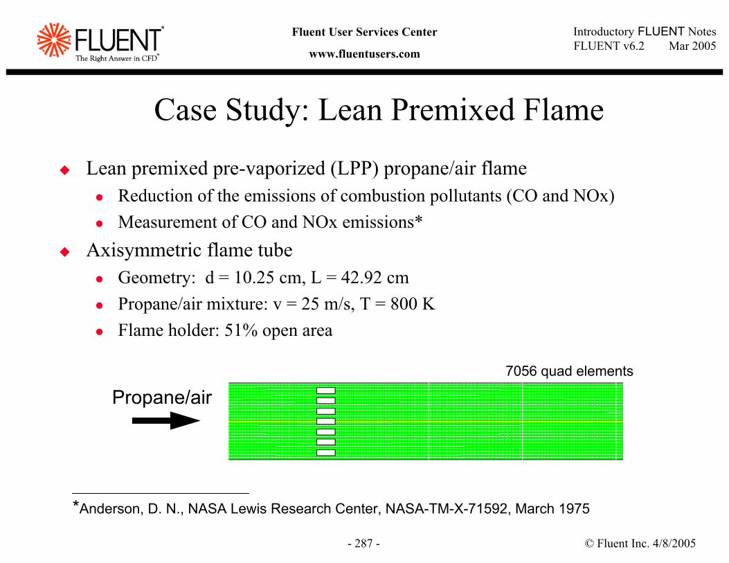
© Fluent Inc. 4/8/2005- 287 -



www.fluentusers.com

Case Study: Lean Premixed Flame

Lean premixed pre-vaporized (LPP) propane/air flameReduction of the emissions of combustion pollutants (CO and NOx)Measurement of CO and NOx emissions*

Axisymmetric flame tubeGeometry: d = 10.25 cm, L = 42.92 cmPropane/air mixture: v = 25 m/s, T = 800 KFlame holder: 51% open area

*Anderson, D. N., NASA Lewis Research Center, NASA-TM-X-71592, March 1975

Propane/air7056 quad elements

© Fluent Inc. 4/8/2005- 288 -



www.fluentusers.com

Weak turbulence-chemistry interactionPerfectly premixedThin flame zoneChemical reactions occur right behind the flame front

Propane detailed chemical mechanismKundu mechanism with NO and N2O formation*

17 species and 23 step reactionsFinite-rate chemistry combustion models

Laminar finite-rate modelFully ignoring turbulence-chemistry interactions

EDC model Might lead to under-prediction of NOx formation: The reaction occurs quickly and NOx has less time to accumulate.

Composition PDF transport Accurately capturing the turbulence-chemistry interaction

Lean Premixed Flame (cont’d)

*Kundu, K. P., et al., NASA Lewis Research Center, AIAA paper 98-3986, July 1998

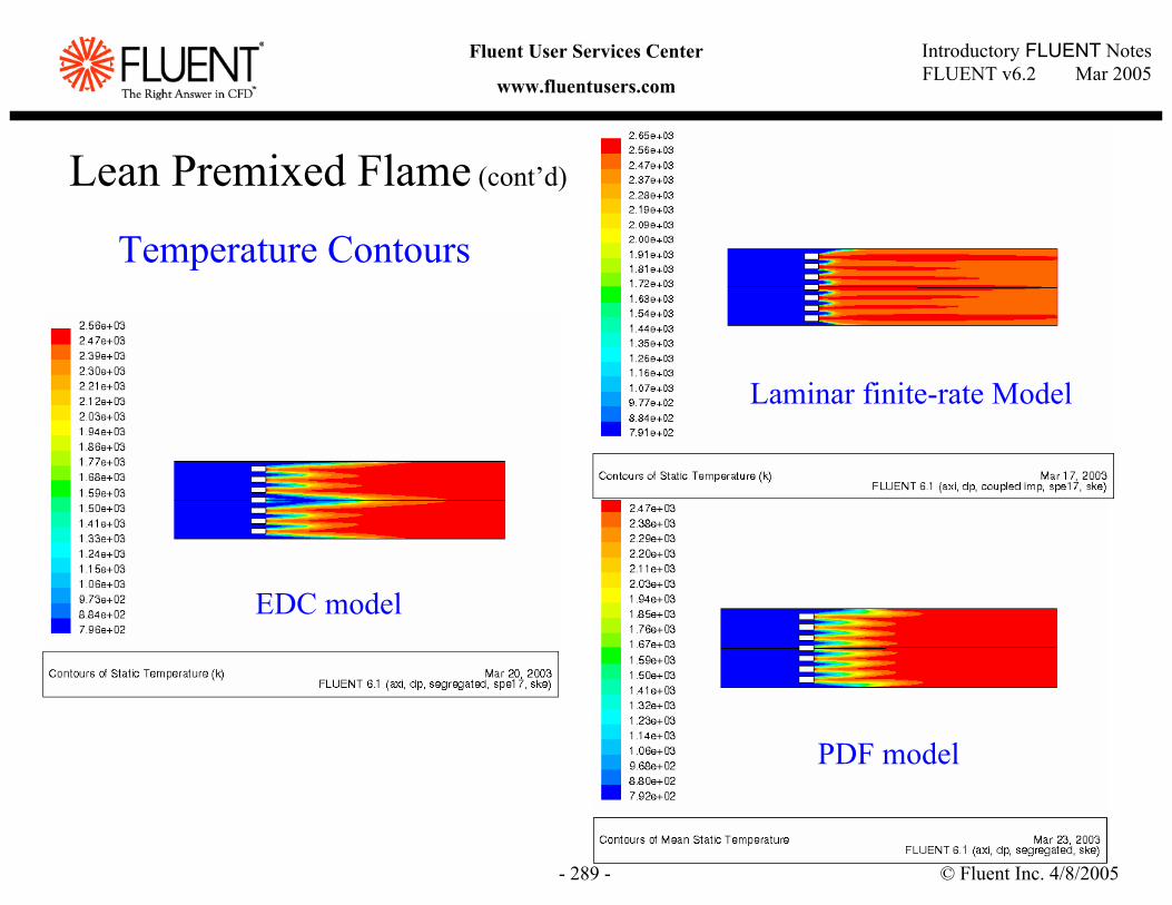
© Fluent Inc. 4/8/2005- 289 -



www.fluentusers.com

Temperature Contours

PDF model

Laminar finite-rate Model

EDC model


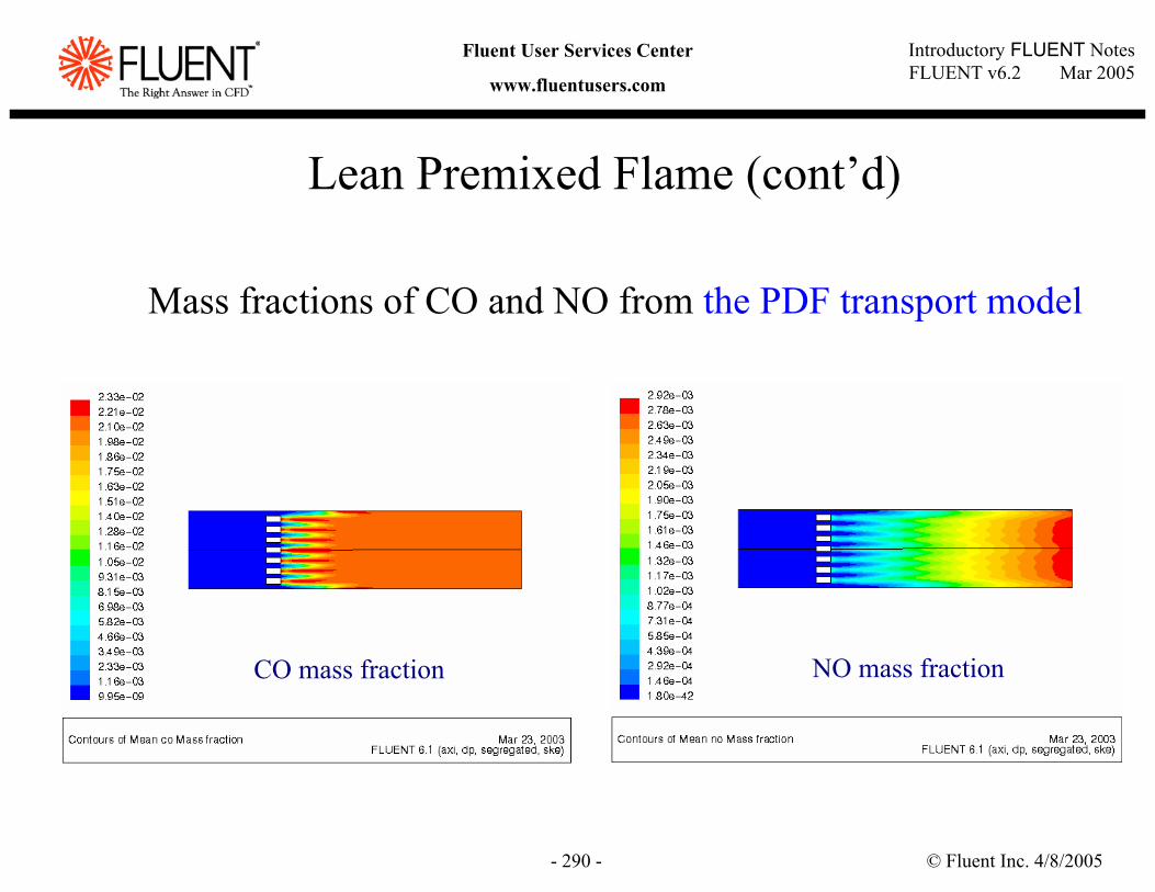
© Fluent Inc. 4/8/2005- 290 -



www.fluentusers.com


Mass fractions of CO and NO from the PDF transport model

CO mass fraction NO mass fraction

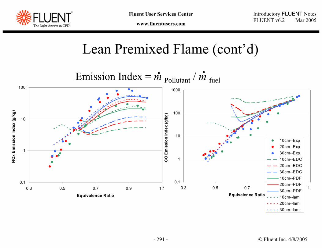
© Fluent Inc. 4/8/2005- 291 -



www.fluentusers.com

0.1

1

10

100

1000

0.3 0.5 0.7 0.9 1.

Equivalence Ratio

CO

Em

issi

on In

dex

(g/k

g)

0.1

1

10

100

0.3 0.5 0.7 0.9 1.1

Equivalence Ratio

NO

x Em

issi

on In

dex

(g/k

g)

10cm--Exp20cm--Exp30cm--Exp10cm--EDC20cm--EDC30cm--EDC10cm--PDF20cm--PDF30cm--PDF10cm--lam20cm--lam30cm--lam

Emission Index = m Pollutant / m fuel

Lean Premixed Flame (cont’d). .

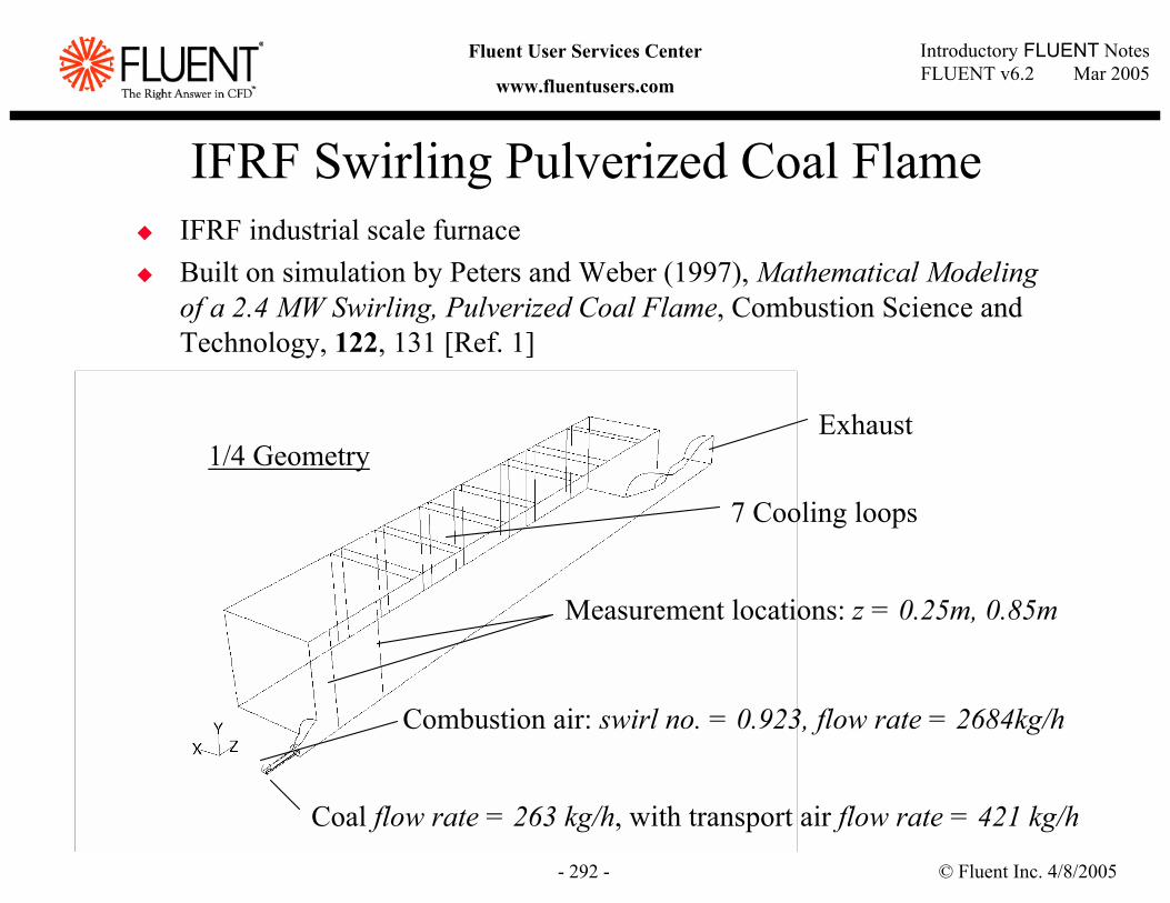
© Fluent Inc. 4/8/2005- 292 -



www.fluentusers.com

IFRF Swirling Pulverized Coal FlameIFRF industrial scale furnaceBuilt on simulation by Peters and Weber (1997), Mathematical Modeling of a 2.4 MW Swirling, Pulverized Coal Flame, Combustion Science and Technology, 122, 131 [Ref. 1]

Exhaust

7 Cooling loops

Measurement locations: z = 0.25m, 0.85m

Combustion air: swirl no. = 0.923, flow rate = 2684kg/h

Coal flow rate = 263 kg/h, with transport air flow rate = 421 kg/h

1/4 Geometry

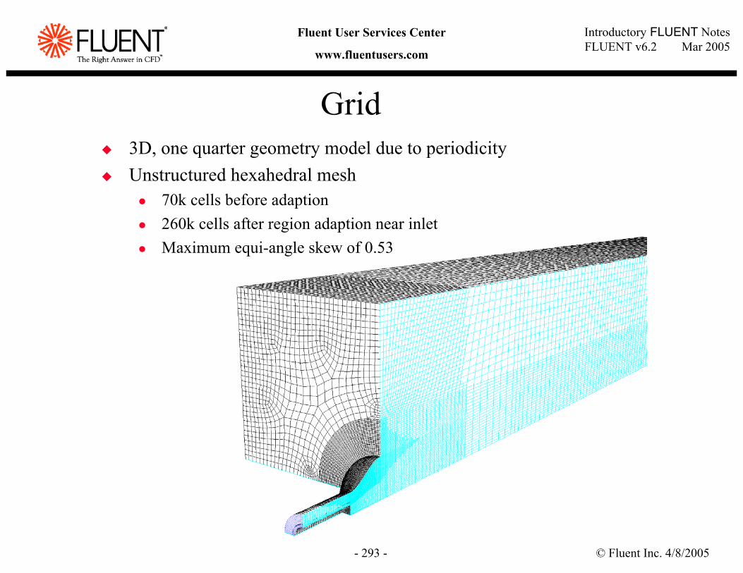
© Fluent Inc. 4/8/2005- 293 -



www.fluentusers.com

Grid3D, one quarter geometry model due to periodicityUnstructured hexahedral mesh

70k cells before adaption260k cells after region adaption near inletMaximum equi-angle skew of 0.53

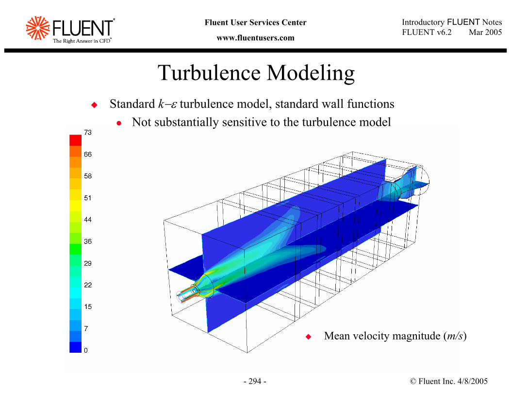
© Fluent Inc. 4/8/2005- 294 -



www.fluentusers.com

Turbulence ModelingStandard k−ε turbulence model, standard wall functions

Not substantially sensitive to the turbulence model

Mean velocity magnitude (m/s)

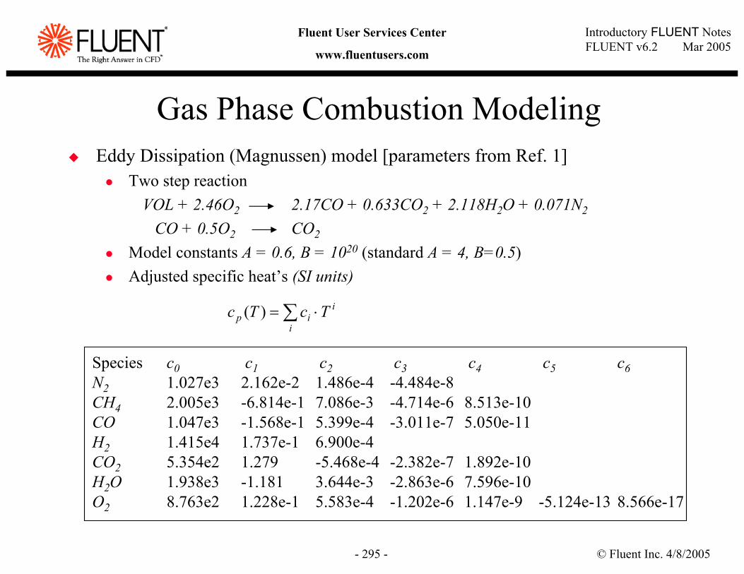
© Fluent Inc. 4/8/2005- 295 -



www.fluentusers.com

Gas Phase Combustion ModelingEddy Dissipation (Magnussen) model [parameters from Ref. 1]

Two step reactionVOL + 2.46O2 2.17CO + 0.633CO2 + 2.118H2O + 0.071N2

CO + 0.5O2 CO2

Model constants A = 0.6, B = 1020 (standard A = 4, B=0.5)Adjusted specific heat’s (SI units)

Species c0 c1 c2 c3 c4 c5 c6N2 1.027e3 2.162e-2 1.486e-4 -4.484e-8CH4 2.005e3 -6.814e-1 7.086e-3 -4.714e-6 8.513e-10CO 1.047e3 -1.568e-1 5.399e-4 -3.011e-7 5.050e-11H2 1.415e4 1.737e-1 6.900e-4CO2 5.354e2 1.279 -5.468e-4 -2.382e-7 1.892e-10 H2O 1.938e3 -1.181 3.644e-3 -2.863e-6 7.596e-10O2 8.763e2 1.228e-1 5.583e-4 -1.202e-6 1.147e-9 -5.124e-13 8.566e-17

∑ ⋅=i

iip TcTc )(

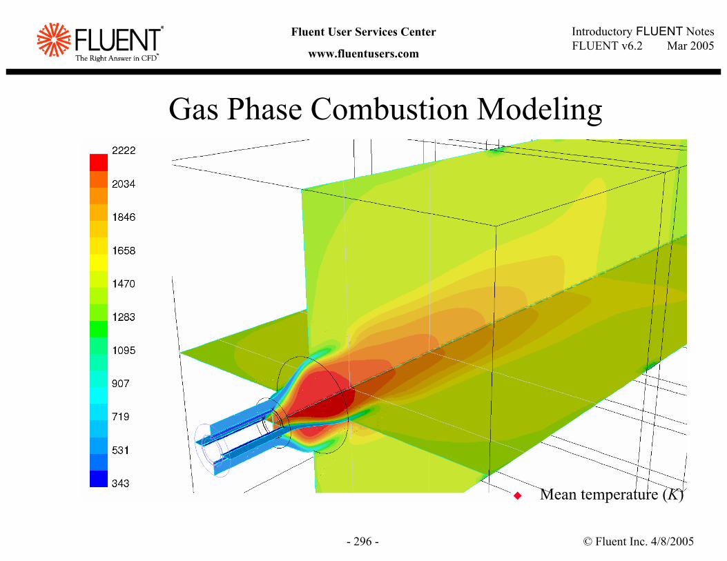
© Fluent Inc. 4/8/2005- 296 -



www.fluentusers.com

Gas Phase Combustion Modeling

Mean temperature (K)

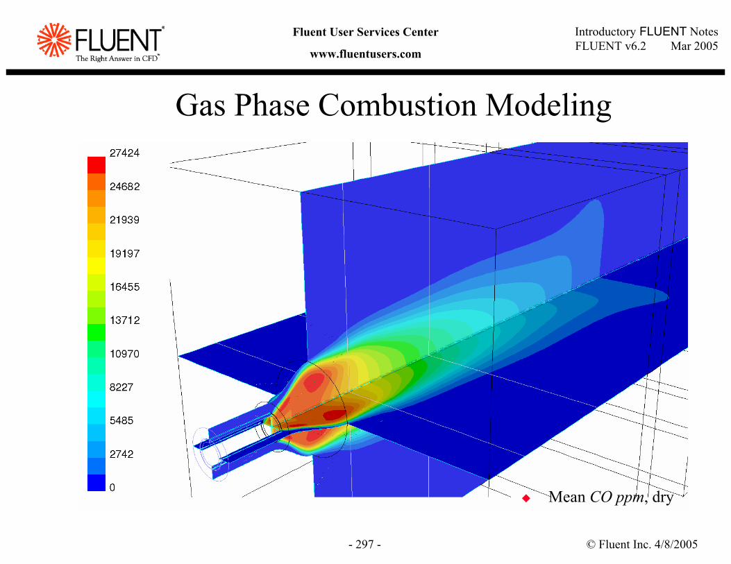
© Fluent Inc. 4/8/2005- 297 -



www.fluentusers.com


Mean CO ppm, dry

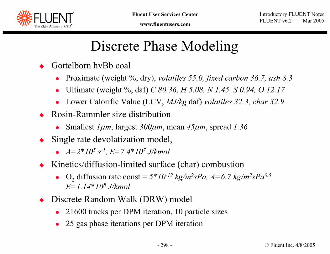
© Fluent Inc. 4/8/2005- 298 -



www.fluentusers.com

Discrete Phase ModelingGottelborn hvBb coal

Proximate (weight %, dry), volatiles 55.0, fixed carbon 36.7, ash 8.3Ultimate (weight %, daf) C 80.36, H 5.08, N 1.45, S 0.94, O 12.17Lower Calorific Value (LCV, MJ/kg daf) volatiles 32.3, char 32.9

Rosin-Rammler size distributionSmallest 1µm, largest 300µm, mean 45µm, spread 1.36

Single rate devolatization model,A=2*105 s-1, E=7.4*107 J/kmol

Kinetics/diffusion-limited surface (char) combustionO2 diffusion rate const = 5*10-12 kg/m2sPa, A=6.7 kg/m2sPa0.5, E=1.14*108 J/kmol

Discrete Random Walk (DRW) model21600 tracks per DPM iteration, 10 particle sizes25 gas phase iterations per DPM iteration

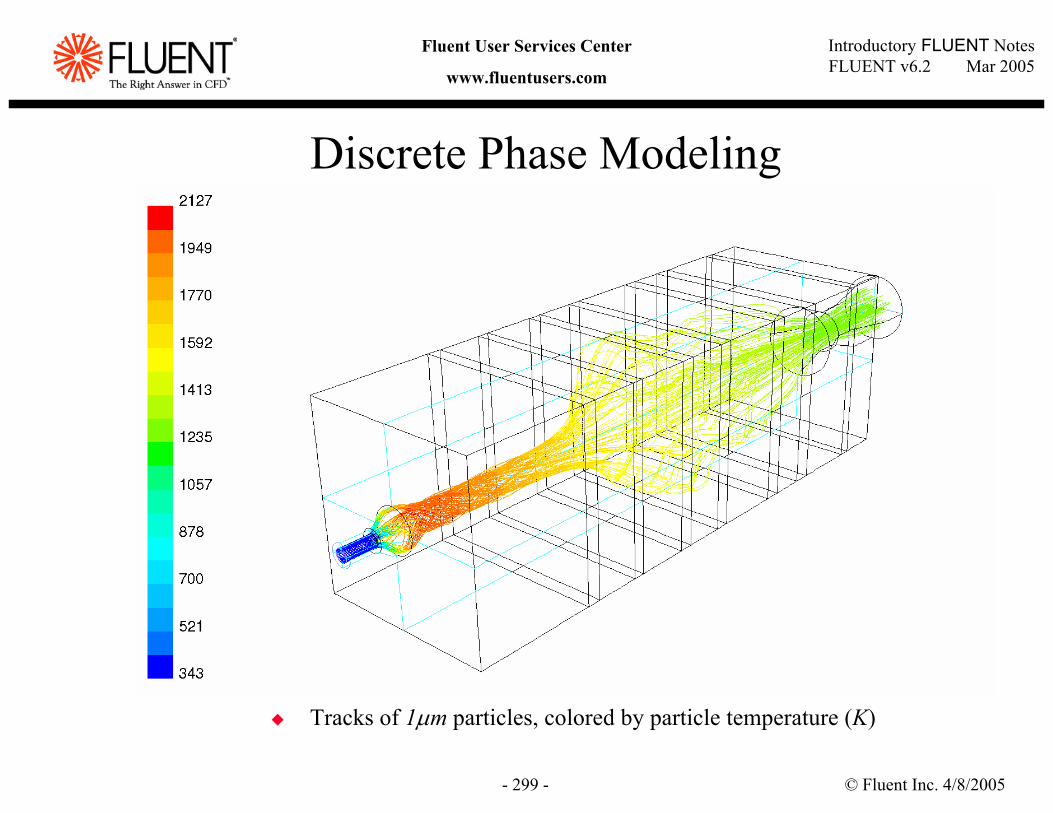
© Fluent Inc. 4/8/2005- 299 -



www.fluentusers.com

Discrete Phase Modeling

Tracks of 1µm particles, colored by particle temperature (K)

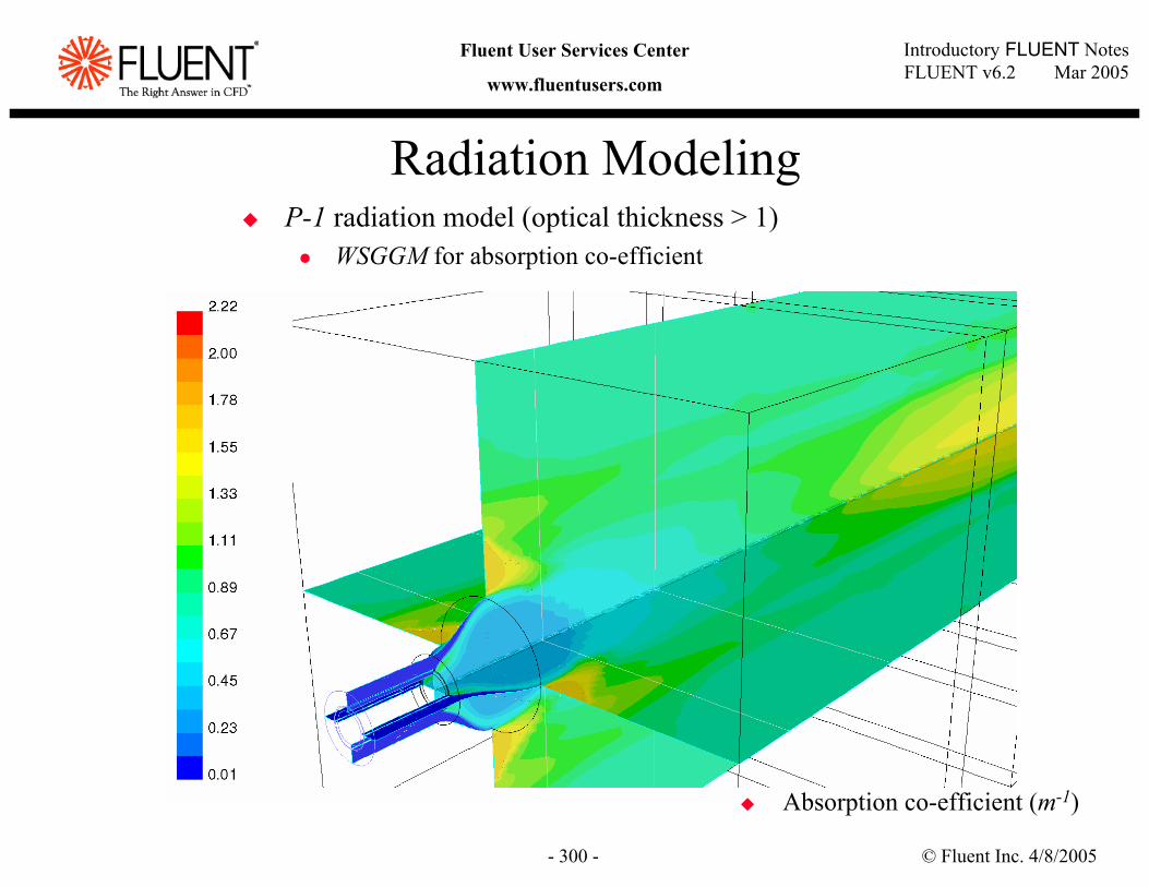
© Fluent Inc. 4/8/2005- 300 -



www.fluentusers.com

Radiation ModelingP-1 radiation model (optical thickness > 1)

WSGGM for absorption co-efficient

Absorption co-efficient (m-1)

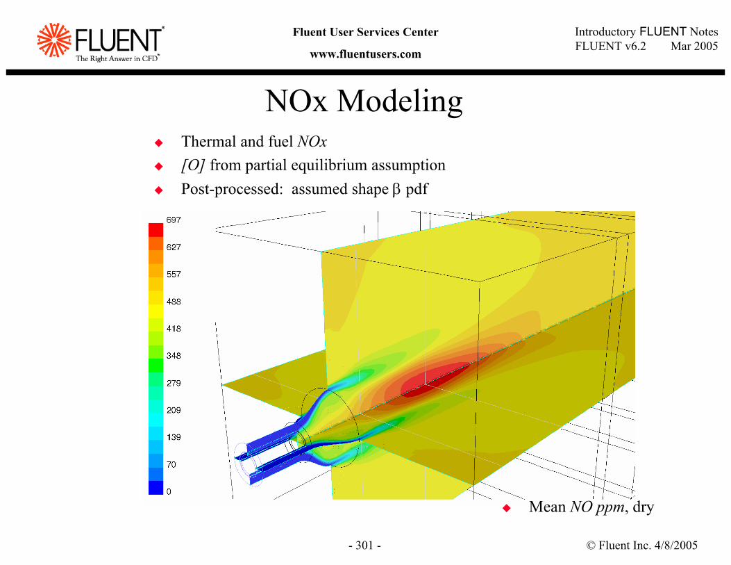
© Fluent Inc. 4/8/2005- 301 -



www.fluentusers.com

NOx ModelingThermal and fuel NOx[O] from partial equilibrium assumptionPost-processed: assumed shape β pdf

Mean NO ppm, dry

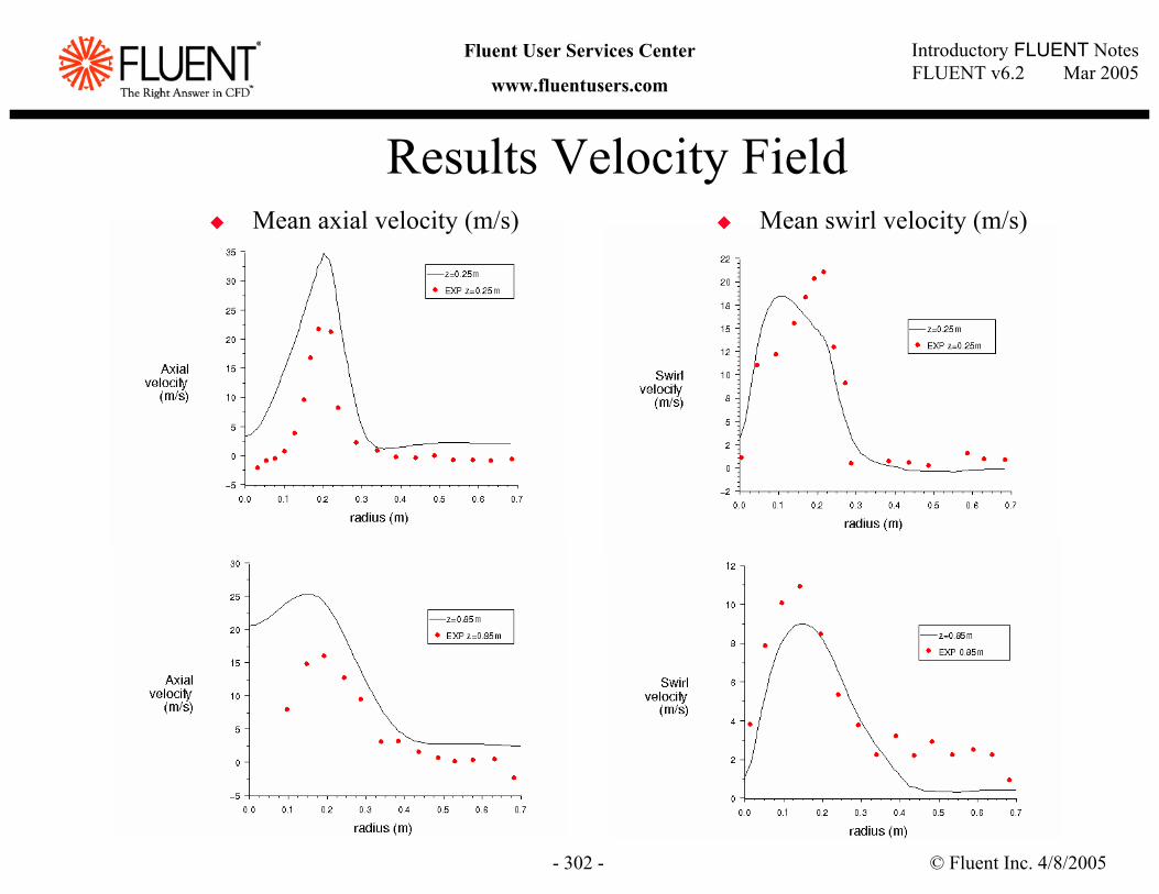
© Fluent Inc. 4/8/2005- 302 -



www.fluentusers.com

Results Velocity FieldMean swirl velocity (m/s)Mean axial velocity (m/s)

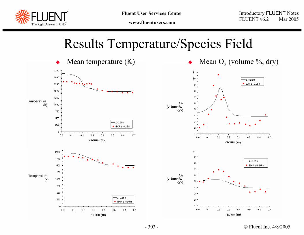
© Fluent Inc. 4/8/2005- 303 -



www.fluentusers.com

Results Temperature/Species FieldMean temperature (K) Mean O2 (volume %, dry)

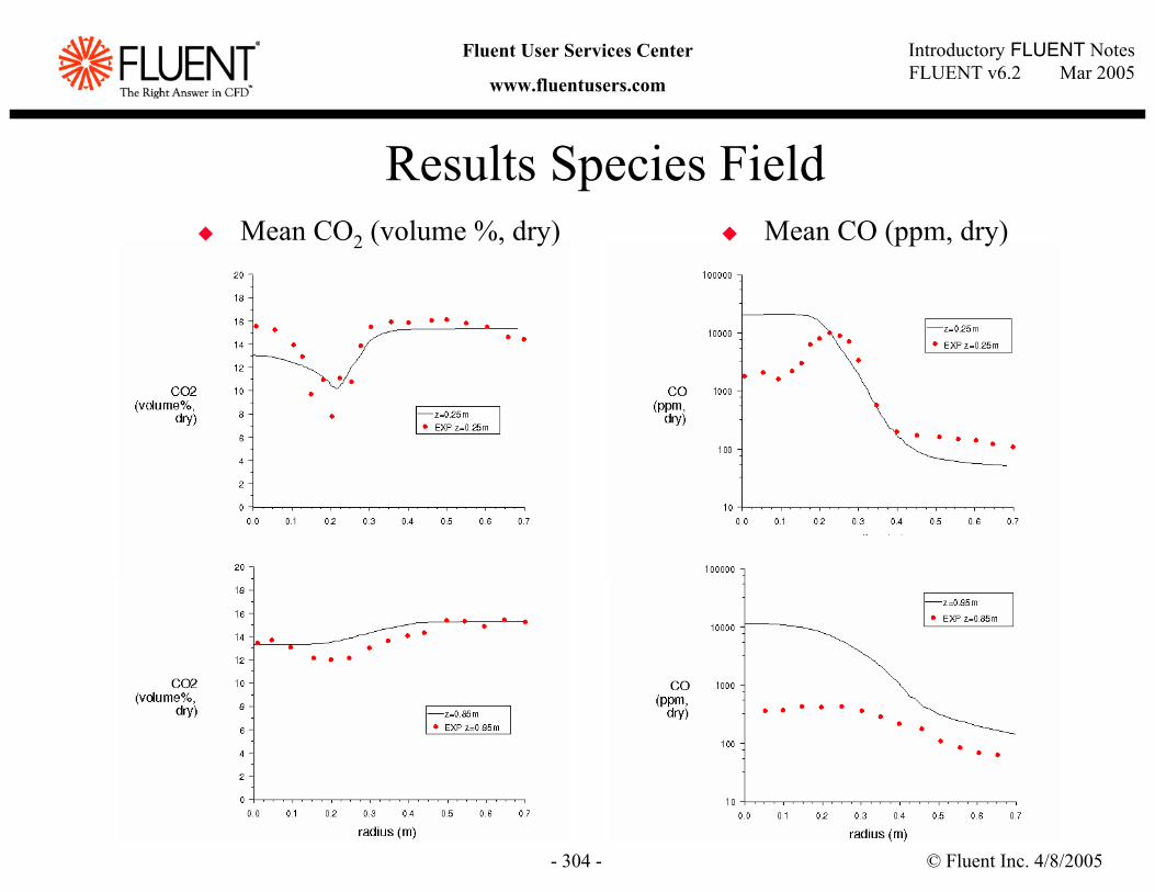
© Fluent Inc. 4/8/2005- 304 -



www.fluentusers.com

Results Species FieldMean CO (ppm, dry)Mean CO2 (volume %, dry)

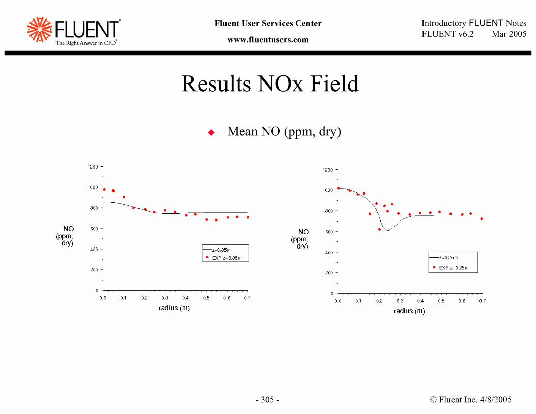
© Fluent Inc. 4/8/2005- 305 -



www.fluentusers.com

Results NOx Field

Mean NO (ppm, dry)

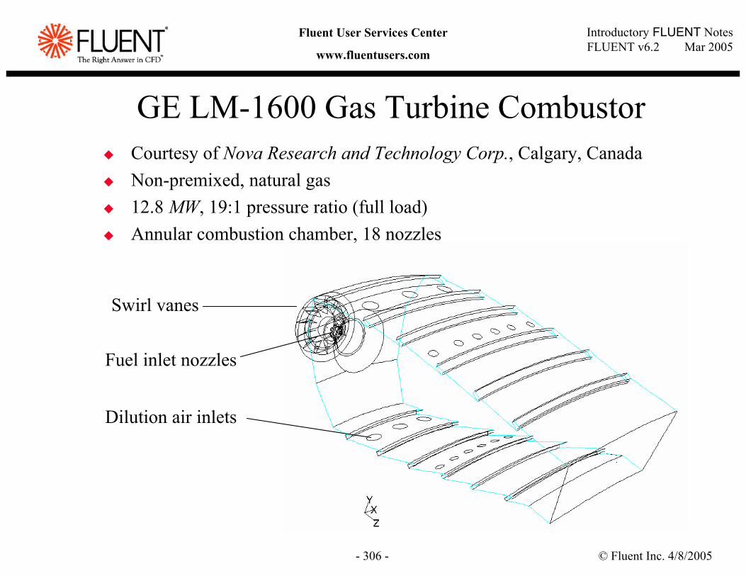
© Fluent Inc. 4/8/2005- 306 -



www.fluentusers.com

GE LM-1600 Gas Turbine CombustorCourtesy of Nova Research and Technology Corp., Calgary, CanadaNon-premixed, natural gas12.8 MW, 19:1 pressure ratio (full load)Annular combustion chamber, 18 nozzles

Swirl vanes

Fuel inlet nozzles

Dilution air inlets

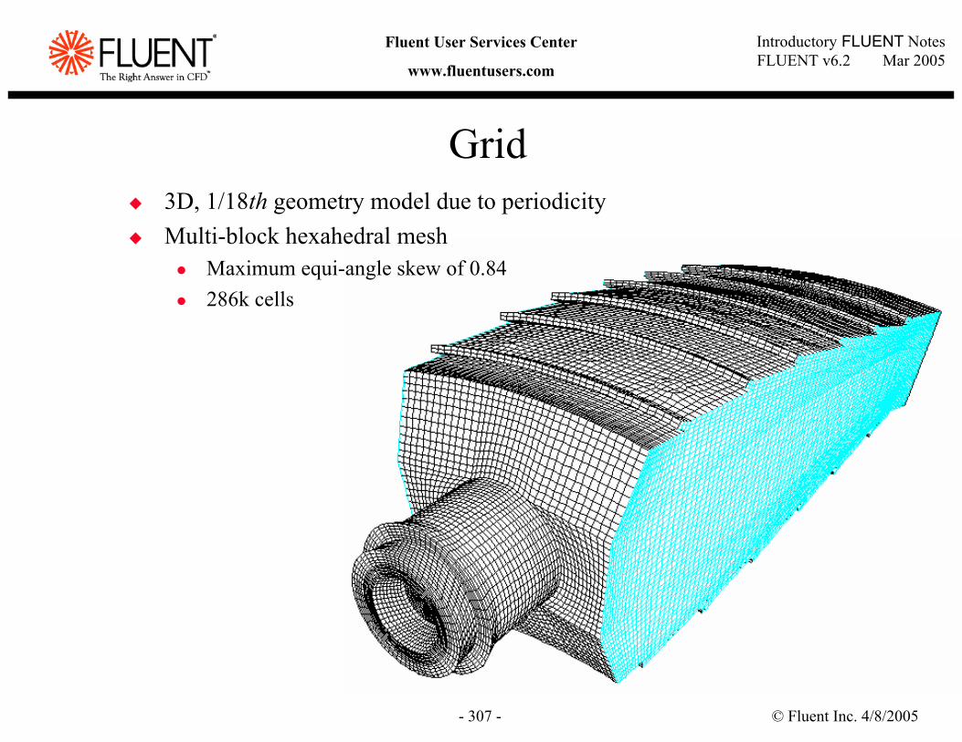
© Fluent Inc. 4/8/2005- 307 -



www.fluentusers.com

Grid3D, 1/18th geometry model due to periodicityMulti-block hexahedral mesh

Maximum equi-angle skew of 0.84286k cells

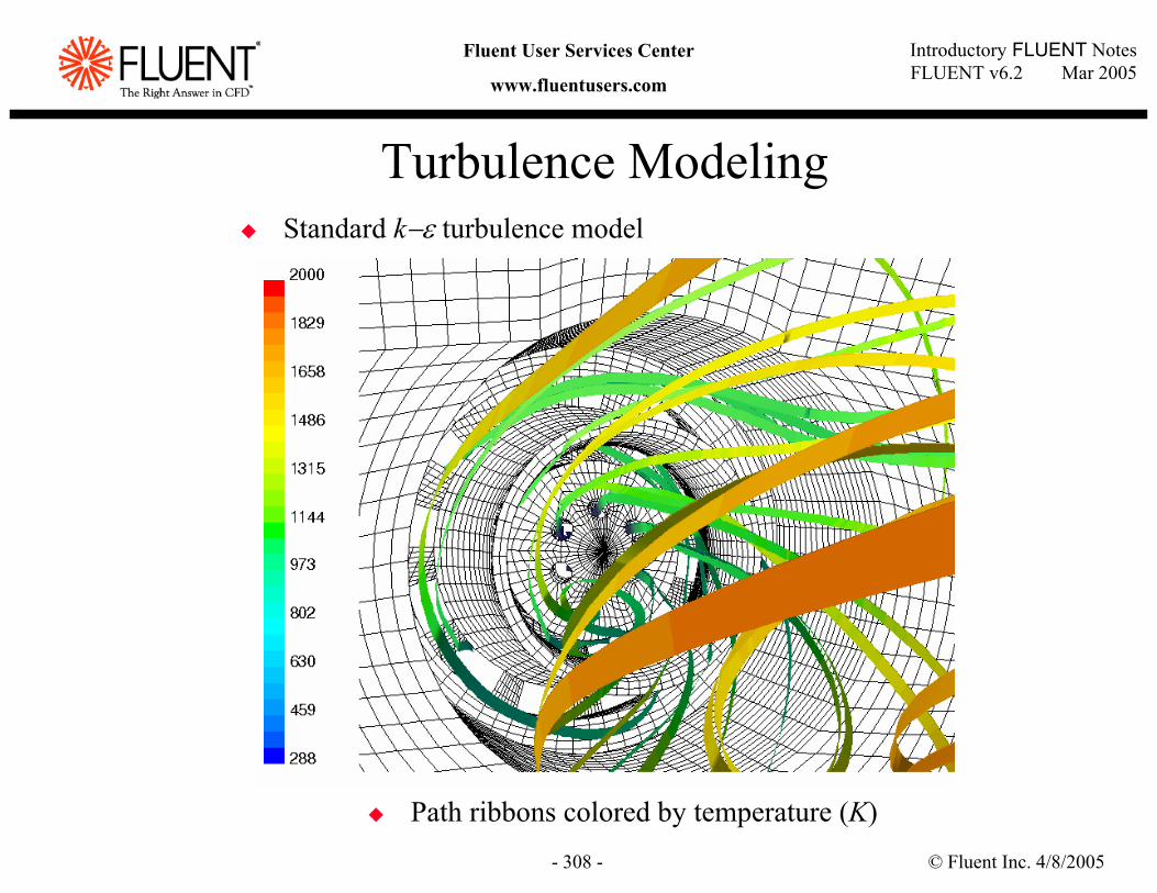
© Fluent Inc. 4/8/2005- 308 -



www.fluentusers.com

Turbulence ModelingStandard k−ε turbulence model

Path ribbons colored by temperature (K)

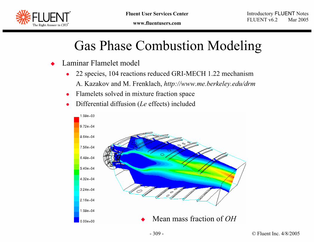
© Fluent Inc. 4/8/2005- 309 -



www.fluentusers.com

Gas Phase Combustion ModelingLaminar Flamelet model

22 species, 104 reactions reduced GRI-MECH 1.22 mechanismA. Kazakov and M. Frenklach, http://www.me.berkeley.edu/drmFlamelets solved in mixture fraction spaceDifferential diffusion (Le effects) included

Mean mass fraction of OH

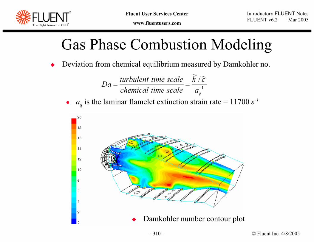
© Fluent Inc. 4/8/2005- 310 -



www.fluentusers.com

Gas Phase Combustion ModelingDeviation from chemical equilibrium measured by Damkohler no.

aq is the laminar flamelet extinction strain rate = 11700 s-1

Damkohler number contour plot

1

~/~−==qa

kscaletimechemicalscaletimeturbulentDa ε

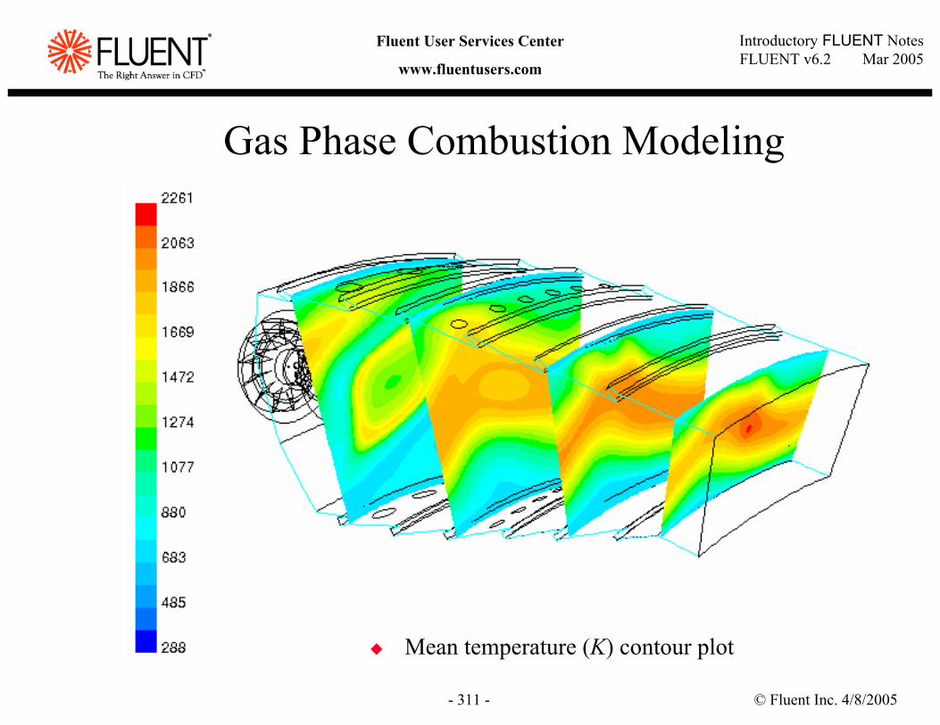
© Fluent Inc. 4/8/2005- 311 -



www.fluentusers.com


Mean temperature (K) contour plot

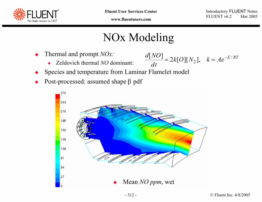
© Fluent Inc. 4/8/2005- 312 -



www.fluentusers.com

NOx ModelingThermal and prompt NOx:

Zeldovich thermal NO dominant:Species and temperature from Laminar Flamelet modelPost-processed: assumed shape β pdf

Mean NO ppm, wet

RTEAekNOktd

NOd /2 ],][[2][ −==

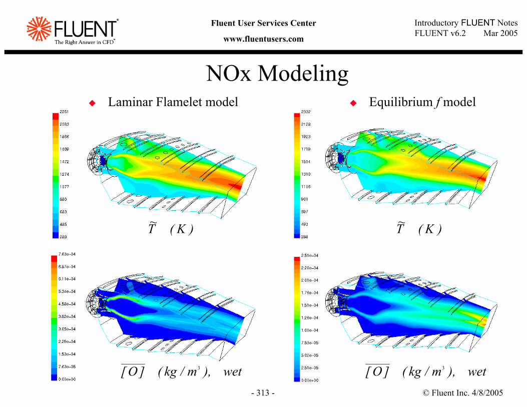
© Fluent Inc. 4/8/2005- 313 -



www.fluentusers.com

NOx ModelingLaminar Flamelet model Equilibrium f model

)K(T~ )K(T~

wet),m/kg(]O[ 3wet),m/kg(]O[ 3

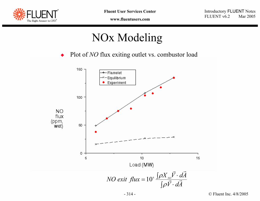
© Fluent Inc. 4/8/2005- 314 -



www.fluentusers.com

NOx ModelingPlot of NO flux exiting outlet vs. combustor load

∫ ⋅∫ ⋅

=AdV

AdVXfluxexitNO NO rr

rr

ρρ610

© Fluent Inc. 4/8/2005- 315 -



www.fluentusers.com

Moving ZonesMoving Zones

© Fluent Inc. 4/8/2005- 316 -



www.fluentusers.com

Outline

Introduction and Overview of Modeling ApproachesSingle-Reference Frame (SRF) ModelMultiple Zones and Multiple-Reference Frame Model (MRF)Mixing Plane Model (MPM)Sliding Mesh Model (SMM)Dynamic Mesh (DM) ModelSummaryAppendix

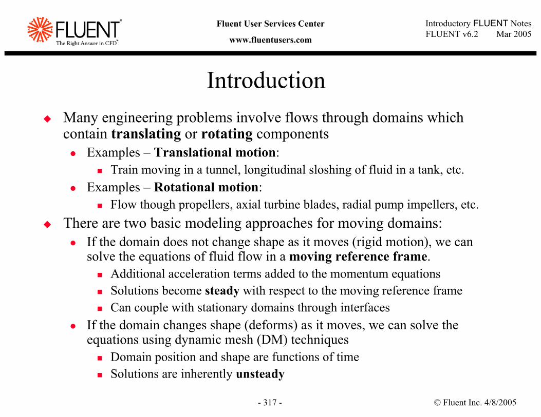
© Fluent Inc. 4/8/2005- 317 -



www.fluentusers.com

IntroductionMany engineering problems involve flows through domains which contain translating or rotating components

Examples – Translational motion:Train moving in a tunnel, longitudinal sloshing of fluid in a tank, etc.

Examples – Rotational motion:Flow though propellers, axial turbine blades, radial pump impellers, etc.

There are two basic modeling approaches for moving domains:If the domain does not change shape as it moves (rigid motion), we can solve the equations of fluid flow in a moving reference frame.

Additional acceleration terms added to the momentum equationsSolutions become steady with respect to the moving reference frameCan couple with stationary domains through interfaces

If the domain changes shape (deforms) as it moves, we can solve the equations using dynamic mesh (DM) techniques

Domain position and shape are functions of timeSolutions are inherently unsteady

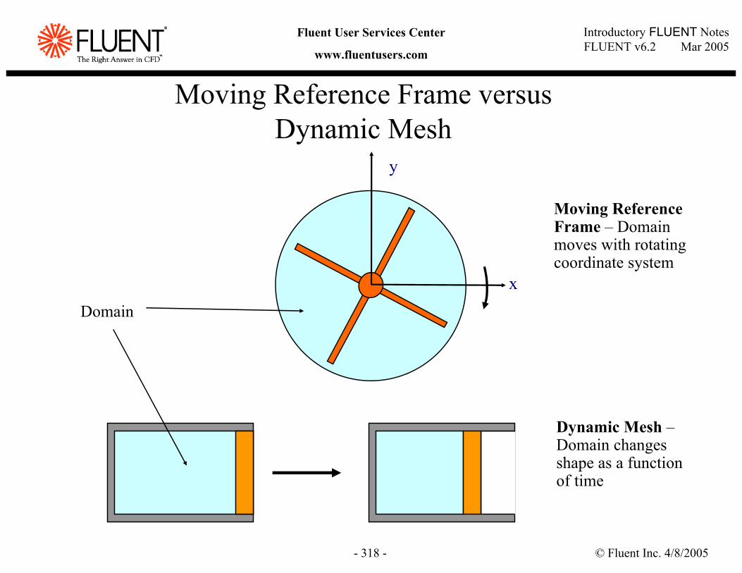
© Fluent Inc. 4/8/2005- 318 -



www.fluentusers.com

xDomain

Moving Reference Frame versusDynamic Mesh

y

Moving Reference Frame – Domain moves with rotating coordinate system

Dynamic Mesh –Domain changes shape as a function of time

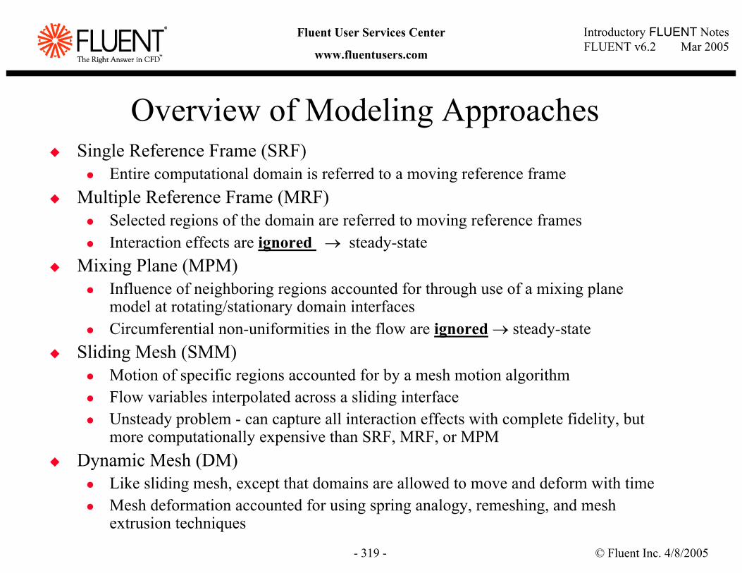
© Fluent Inc. 4/8/2005- 319 -



www.fluentusers.com

Overview of Modeling ApproachesSingle Reference Frame (SRF)

Entire computational domain is referred to a moving reference frameMultiple Reference Frame (MRF)

Selected regions of the domain are referred to moving reference framesInteraction effects are ignored → steady-state

Mixing Plane (MPM)Influence of neighboring regions accounted for through use of a mixing plane model at rotating/stationary domain interfacesCircumferential non-uniformities in the flow are ignored → steady-state

Sliding Mesh (SMM)Motion of specific regions accounted for by a mesh motion algorithm Flow variables interpolated across a sliding interfaceUnsteady problem - can capture all interaction effects with complete fidelity, butmore computationally expensive than SRF, MRF, or MPM

Dynamic Mesh (DM)Like sliding mesh, except that domains are allowed to move and deform with timeMesh deformation accounted for using spring analogy, remeshing, and mesh extrusion techniques

© Fluent Inc. 4/8/2005- 320 -



www.fluentusers.com

Outline


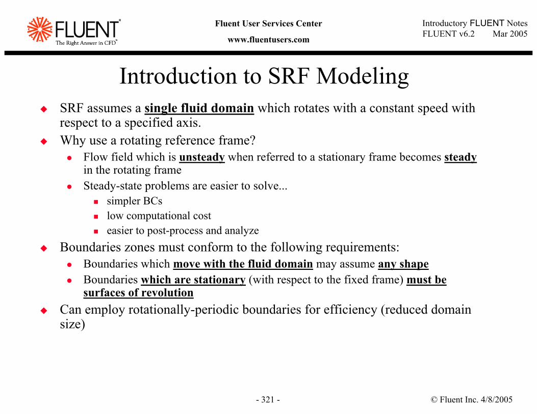
© Fluent Inc. 4/8/2005- 321 -



www.fluentusers.com

Introduction to SRF ModelingSRF assumes a single fluid domain which rotates with a constant speed with respect to a specified axis.Why use a rotating reference frame?

Flow field which is unsteady when referred to a stationary frame becomes steadyin the rotating frameSteady-state problems are easier to solve...

simpler BCslow computational costeasier to post-process and analyze

Boundaries zones must conform to the following requirements:Boundaries which move with the fluid domain may assume any shapeBoundaries which are stationary (with respect to the fixed frame) must be surfaces of revolution

Can employ rotationally-periodic boundaries for efficiency (reduced domain size)

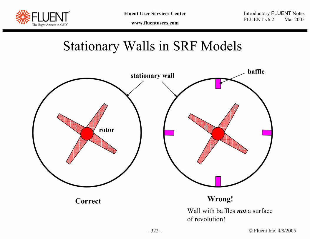
© Fluent Inc. 4/8/2005- 322 -



www.fluentusers.com

Stationary Walls in SRF Models

stationary wall

rotor

baffle

Correct Wrong! Wall with baffles not a surfaceof revolution!

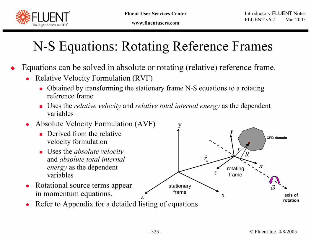
© Fluent Inc. 4/8/2005- 323 -



www.fluentusers.com

N-S Equations: Rotating Reference FramesEquations can be solved in absolute or rotating (relative) reference frame.

Relative Velocity Formulation (RVF)Obtained by transforming the stationary frame N-S equations to a rotating reference frameUses the relative velocity and relative total internal energy as the dependent variables

Absolute Velocity Formulation (AVF)Derived from the relative velocity formulationUses the absolute velocity and absolute total internal energy as the dependent variables

Rotational source terms appear in momentum equations.Refer to Appendix for a detailed listing of equations

x

y

z

z

y

x

stationaryframe

rotatingframe

axis ofrotation

rr

ωr

CFD domain

orr R

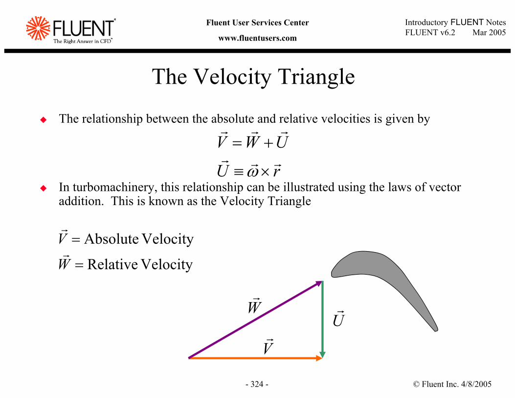
© Fluent Inc. 4/8/2005- 324 -



www.fluentusers.com

The Velocity Triangle

The relationship between the absolute and relative velocities is given by

In turbomachinery, this relationship can be illustrated using the laws of vector addition. This is known as the Velocity Triangle

rU

UWVrrr

rrr

×≡

+=

ω

Vr

Wr

Ur

Velocity Relative

Velocity Absolute

=

=

W

Vr

r

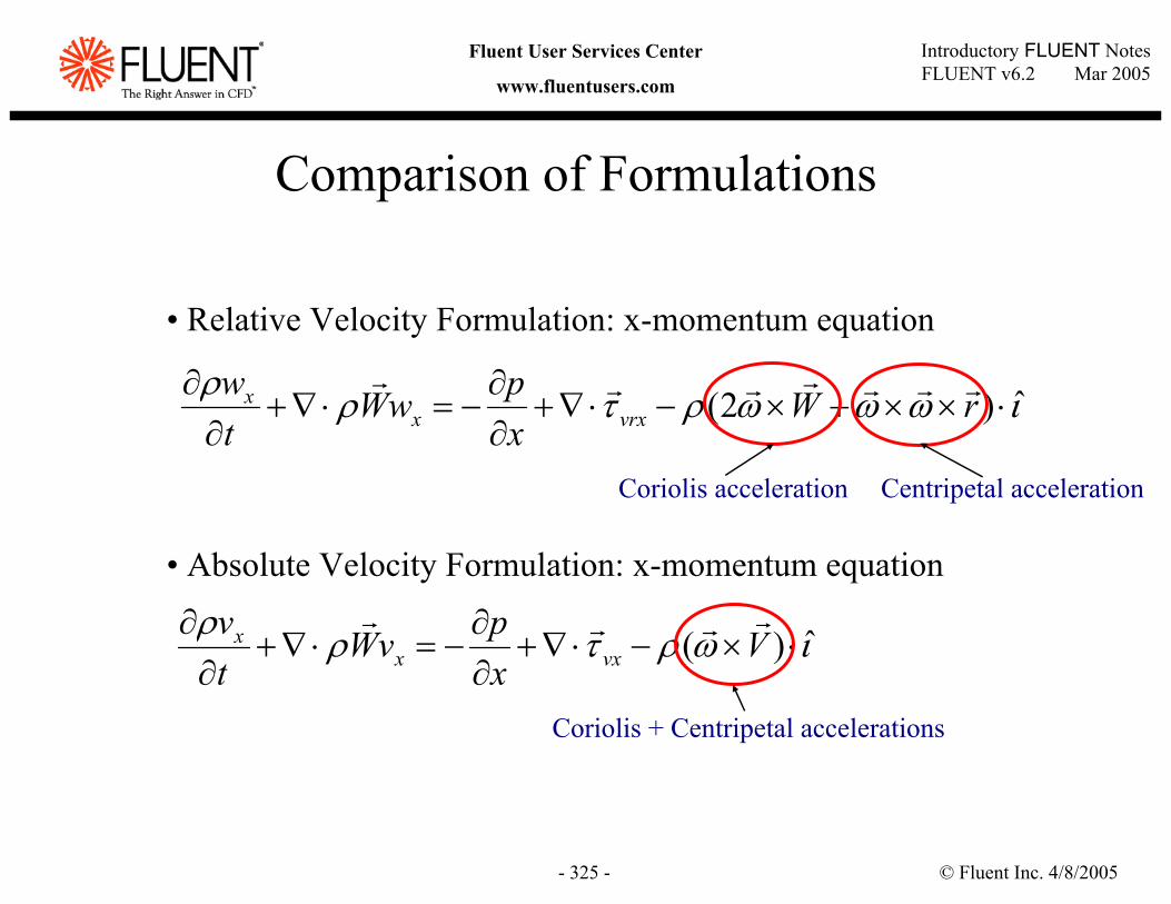
© Fluent Inc. 4/8/2005- 325 -



www.fluentusers.com

Comparison of Formulations

ιωωωρτρρ ˆ)2( ⋅××+×−⋅∇+∂∂

−=⋅∇+∂

∂ rWxpwW

tw

vrxxx rrrrrrr

• Relative Velocity Formulation: x-momentum equation

ιωρτρρ ˆ)( ⋅×−⋅∇+∂∂

−=⋅∇+∂

∂ VxpvW

tv

vxxx

rrrr

• Absolute Velocity Formulation: x-momentum equation

Coriolis acceleration Centripetal acceleration

Coriolis + Centripetal accelerations

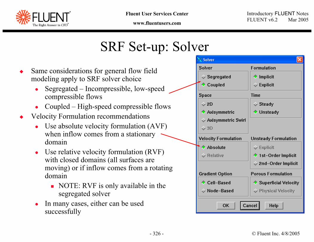
© Fluent Inc. 4/8/2005- 326 -



www.fluentusers.com

SRF Set-up: SolverSame considerations for general flow field modeling apply to SRF solver choice

Segregated – Incompressible, low-speed compressible flowsCoupled – High-speed compressible flows

Velocity Formulation recommendationsUse absolute velocity formulation (AVF) when inflow comes from a stationary domainUse relative velocity formulation (RVF) with closed domains (all surfaces are moving) or if inflow comes from a rotating domain

NOTE: RVF is only available in the segregated solver

In many cases, either can be used successfully

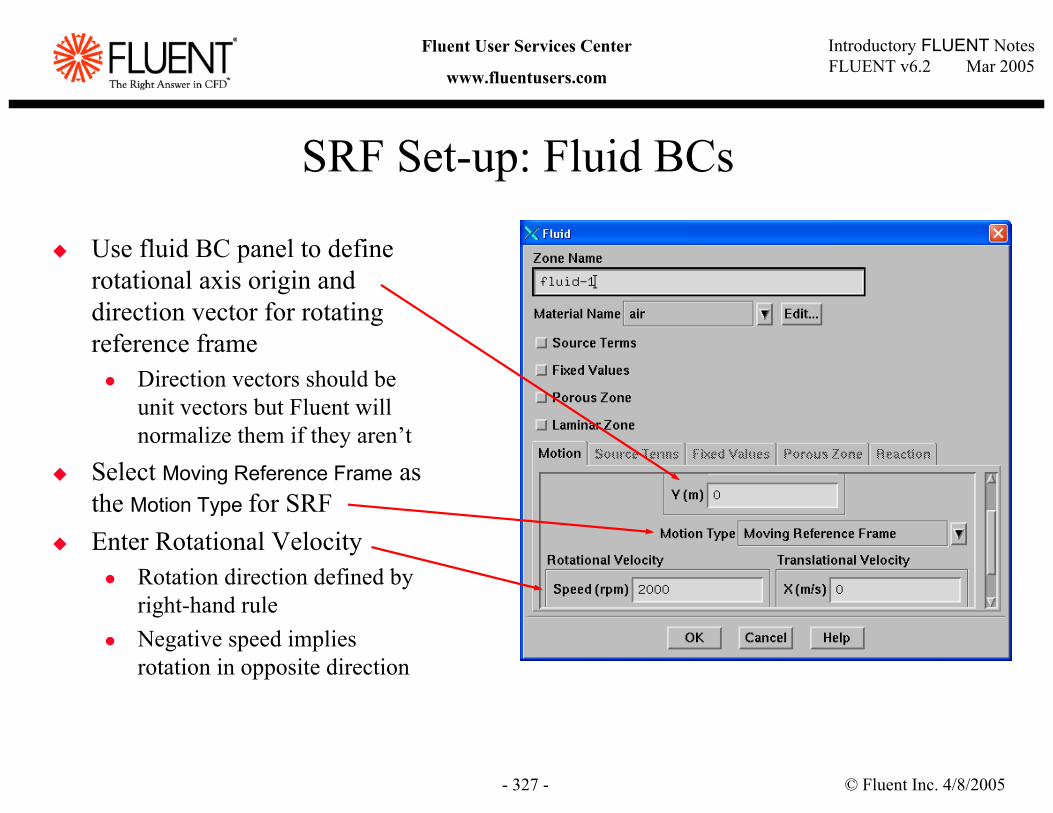
© Fluent Inc. 4/8/2005- 327 -



www.fluentusers.com

SRF Set-up: Fluid BCs

Use fluid BC panel to define rotational axis origin and direction vector for rotating reference frame

Direction vectors should be unit vectors but Fluent will normalize them if they aren’t

Select Moving Reference Frame as the Motion Type for SRFEnter Rotational Velocity

Rotation direction defined by right-hand ruleNegative speed implies rotation in opposite direction

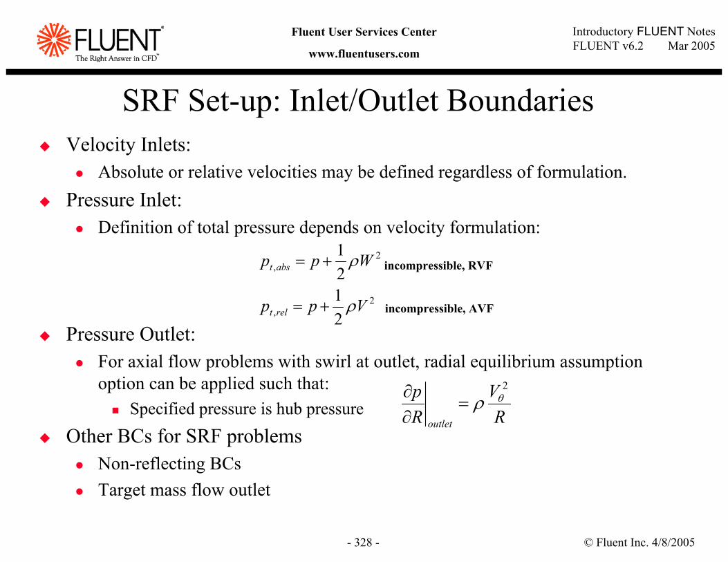
© Fluent Inc. 4/8/2005- 328 -



www.fluentusers.com

SRF Set-up: Inlet/Outlet BoundariesVelocity Inlets:

Absolute or relative velocities may be defined regardless of formulation.Pressure Inlet:

Definition of total pressure depends on velocity formulation:

Pressure Outlet:For axial flow problems with swirl at outlet, radial equilibrium assumption option can be applied such that:

Specified pressure is hub pressure

Other BCs for SRF problemsNon-reflecting BCsTarget mass flow outlet

2,

2,

2121

Vpp

Wpp

relt

abst

ρ

ρ

+=

+=

incompressible, AVF

RV

Rp

outlet

2θρ=

∂∂

incompressible, RVF

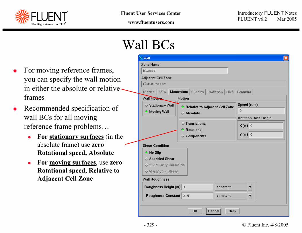
© Fluent Inc. 4/8/2005- 329 -



www.fluentusers.com

Wall BCs

For moving reference frames, you can specify the wall motion in either the absolute or relative framesRecommended specification of wall BCs for all moving reference frame problems…

For stationary surfaces (in the absolute frame) use zero Rotational speed, AbsoluteFor moving surfaces, use zero Rotational speed, Relative to Adjacent Cell Zone

© Fluent Inc. 4/8/2005- 330 -



www.fluentusers.com

Solution Strategies for SRF ProblemsHigh degree of coupling between momentum equations when rotational terms are large can make convergence difficult.Strategies

Ensure that the mesh is sufficiently refined to resolve large gradients in pressure and swirl velocity. Use reasonable values for initial conditions

New in Fluent 6.2: FMG initialization – provides Euler solution as initial condition using the coupled-explicit solver (good for rotating machinery problems)

Begin the calculations using a low rotational speed, increasing the rotational speed gradually in order to reach the final desired operating condition.Begin calculations using first order discretization and switch to second order.For the Segregated solver

Use the PRESTO! Or Body-Force Weighted schemes which are well-suited for the steep pressure gradients involved in rotating flows. Reduce the under-relaxation factors for the velocities, perhaps to 0.3-0.5.

© Fluent Inc. 4/8/2005- 331 -



www.fluentusers.com

Outline


© Fluent Inc. 4/8/2005- 332 -



www.fluentusers.com

Multiple Zone Modeling

Many rotating machinery problems involve stationary components which cannot be described by surfaces of revolution (SRF not valid).Systems like these can be solved by dividing the domain into multiplefluid zones – some zones will be rotating, others stationary.For multiple zone models, we can apply one of the following approaches:

Multiple reference frame model (MRF)Simplified interface treatment - rotational interaction between reference frames is not accounted for.

Mixing plane model (MPM)Interaction between reference frames are approximated through circumferential averaging at fluid zone interfaces (mixing planes).

Sliding mesh model (SMM)Accurately models the relative motion between moving and stationary zones at the expense of more CPU time (inherently unsteady).

© Fluent Inc. 4/8/2005- 333 -



www.fluentusers.com

Introduction to the MRF ModelThe domain is subdivided into stationary and rotating fluid zones.

More than one rotating zone is permitted.Zones can rotate at different speeds.

Governing equations are solved in each fluid zone.SRF equations used in rotating zones.At the interfaces between the rotating and stationary zones, appropriate transformations of the velocity vector and velocity gradients are performed to compute fluxes of mass, momentum, energy, and other scalars.Flow is assumed to be steady in each zone (clearly an approximation).

MRF ignores the relative motions of the zones with respect to each other.Does not account for fluid dynamic interaction between stationary and rotating components.For this reason MRF is often referred to as the “frozen rotor” approach.

Ideally, the flow at the MRF interfaces should be relatively uniform or “mixed out.”

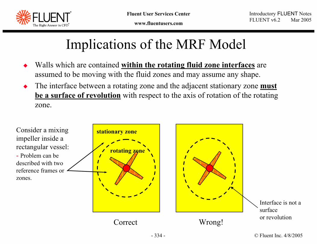
© Fluent Inc. 4/8/2005- 334 -



www.fluentusers.com

Implications of the MRF ModelWalls which are contained within the rotating fluid zone interfaces are assumed to be moving with the fluid zones and may assume any shape.The interface between a rotating zone and the adjacent stationary zone must be a surface of revolution with respect to the axis of rotation of the rotating zone.

Correct Wrong!

Interface is not a surface or revolution

stationary zone

rotating zone

Consider a mixing impeller inside a rectangular vessel:- Problem can be described with two reference frames or zones.

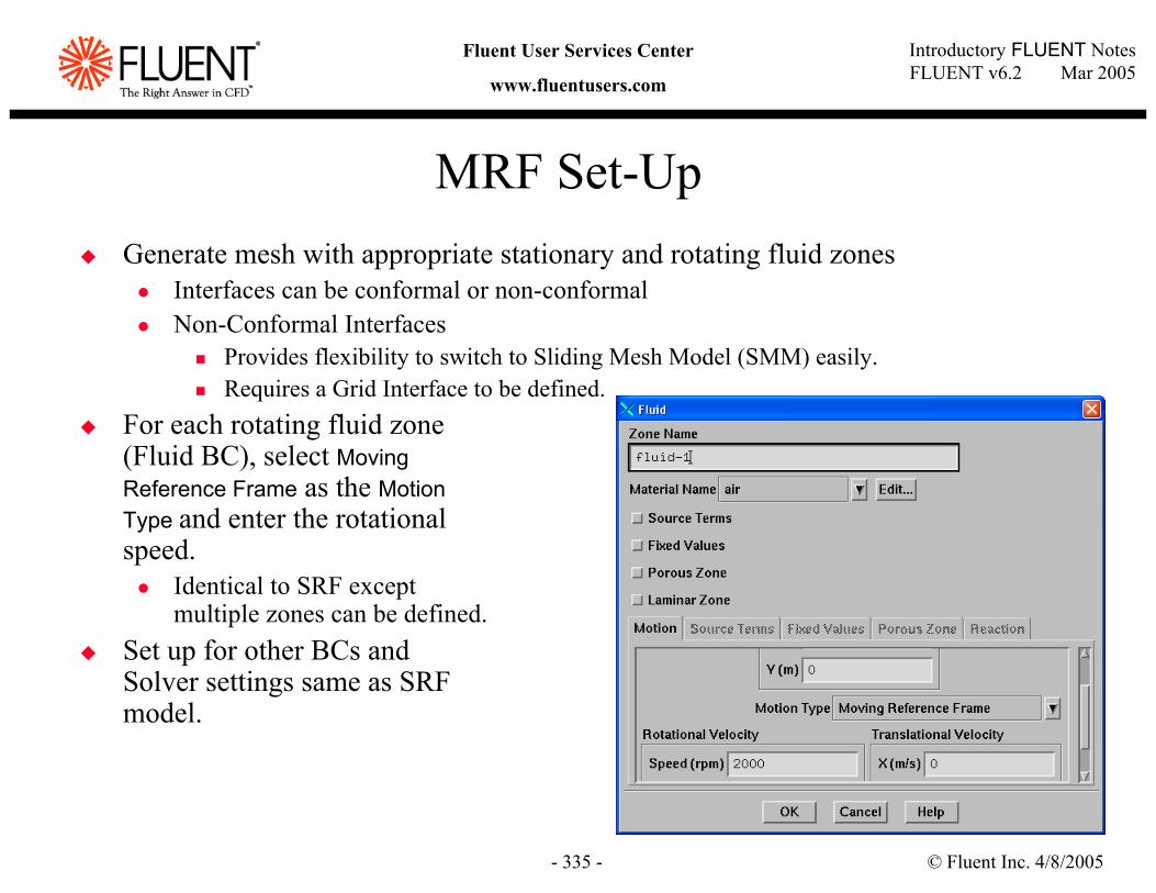
© Fluent Inc. 4/8/2005- 335 -



www.fluentusers.com

MRF Set-UpGenerate mesh with appropriate stationary and rotating fluid zones

Interfaces can be conformal or non-conformalNon-Conformal Interfaces

Provides flexibility to switch to Sliding Mesh Model (SMM) easily.Requires a Grid Interface to be defined.

For each rotating fluid zone (Fluid BC), select Moving Reference Frame as the Motion Type and enter the rotational speed.

Identical to SRF except multiple zones can be defined.

Set up for other BCs and Solver settings same as SRF model.

© Fluent Inc. 4/8/2005- 336 -



www.fluentusers.com

Outline


© Fluent Inc. 4/8/2005- 337 -



www.fluentusers.com

Introduction to Mixing Plane Model (MPM)The MPM was originally implemented to accommodate rotor/stator and impeller/vane flows in axial and centrifugal turbomachines.

Can also be applied to a more general class of problems.Typically, the domain is divided into rotating and stationary zones that correspond to the rotors and stators.

Multiple rotor/stator ‘stages’ are allowed.Governing equations are solved in each domain.

Flow is assumed steady in each domain.The interfaces between the domains are called the mixing planes.Circumferentially averaged profiles of flow variables are computed at the mixing planes.The profiles are used as boundary conditions to the adjacent domains.As the solution converges, the mixing plane boundary conditions will adjust to the prevailing flow conditions.

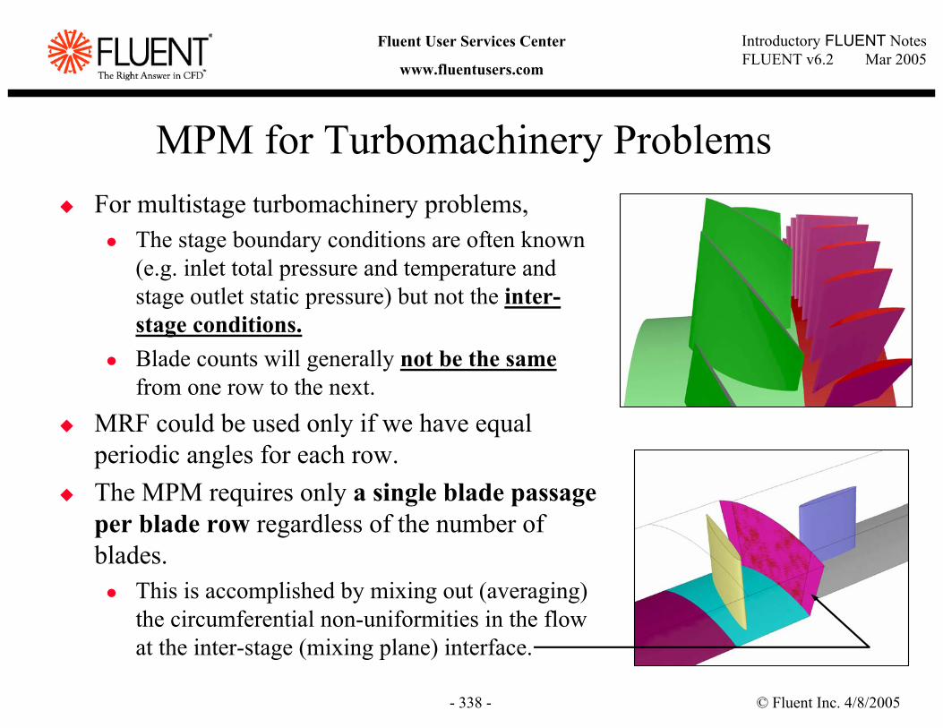
© Fluent Inc. 4/8/2005- 338 -



www.fluentusers.com

MPM for Turbomachinery ProblemsFor multistage turbomachinery problems,

The stage boundary conditions are often known (e.g. inlet total pressure and temperature and stage outlet static pressure) but not the inter-stage conditions.Blade counts will generally not be the samefrom one row to the next.

MRF could be used only if we have equal periodic angles for each row.The MPM requires only a single blade passage per blade row regardless of the number of blades.

This is accomplished by mixing out (averaging) the circumferential non-uniformities in the flow at the inter-stage (mixing plane) interface.

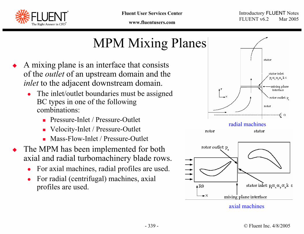
© Fluent Inc. 4/8/2005- 339 -



www.fluentusers.com

MPM Mixing Planes

axial machines

radial machines

A mixing plane is an interface that consists of the outlet of an upstream domain and the inlet to the adjacent downstream domain.

The inlet/outlet boundaries must be assigned BC types in one of the following combinations:

Pressure-Inlet / Pressure-OutletVelocity-Inlet / Pressure-Outlet Mass-Flow-Inlet / Pressure-Outlet

The MPM has been implemented for both axial and radial turbomachinery blade rows.

For axial machines, radial profiles are used.For radial (centrifugal) machines, axial profiles are used.

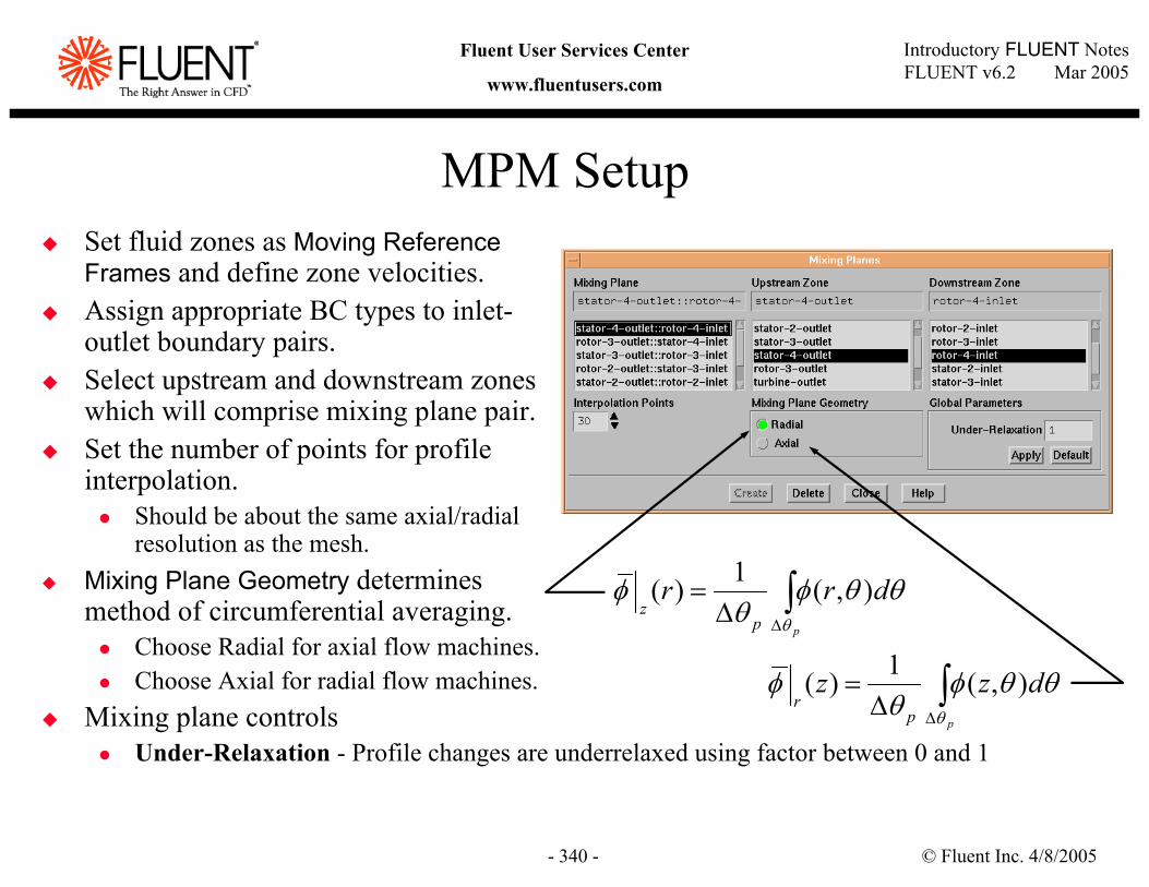
© Fluent Inc. 4/8/2005- 340 -



www.fluentusers.com

MPM SetupSet fluid zones as Moving ReferenceFrames and define zone velocities.Assign appropriate BC types to inlet-outlet boundary pairs.Select upstream and downstream zones which will comprise mixing plane pair.Set the number of points for profile interpolation.

Should be about the same axial/radial resolution as the mesh.

Mixing Plane Geometry determinesmethod of circumferential averaging.

Choose Radial for axial flow machines.Choose Axial for radial flow machines.

Mixing plane controlsUnder-Relaxation - Profile changes are underrelaxed using factor between 0 and 1

∫∆∆

=p

drrp

zθ

θθφθ

φ ),(1)(

∫∆∆

=p

dzzp

rθ

θθφθ

φ ),(1)(

© Fluent Inc. 4/8/2005- 341 -



www.fluentusers.com

Outline


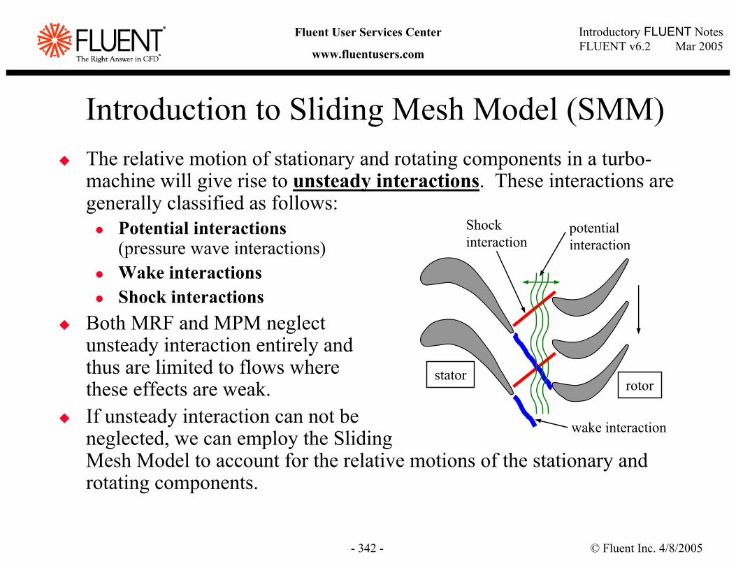
© Fluent Inc. 4/8/2005- 342 -



www.fluentusers.com

Introduction to Sliding Mesh Model (SMM)The relative motion of stationary and rotating components in a turbo-machine will give rise to unsteady interactions. These interactions are generally classified as follows:

Potential interactions(pressure wave interactions)Wake interactionsShock interactions

Both MRF and MPM neglect unsteady interaction entirely and thus are limited to flows where these effects are weak.If unsteady interaction can not be neglected, we can employ the SlidingMesh Model to account for the relative motions of the stationary and rotating components.

wake interaction

Shockinteraction

potential interaction

statorrotor

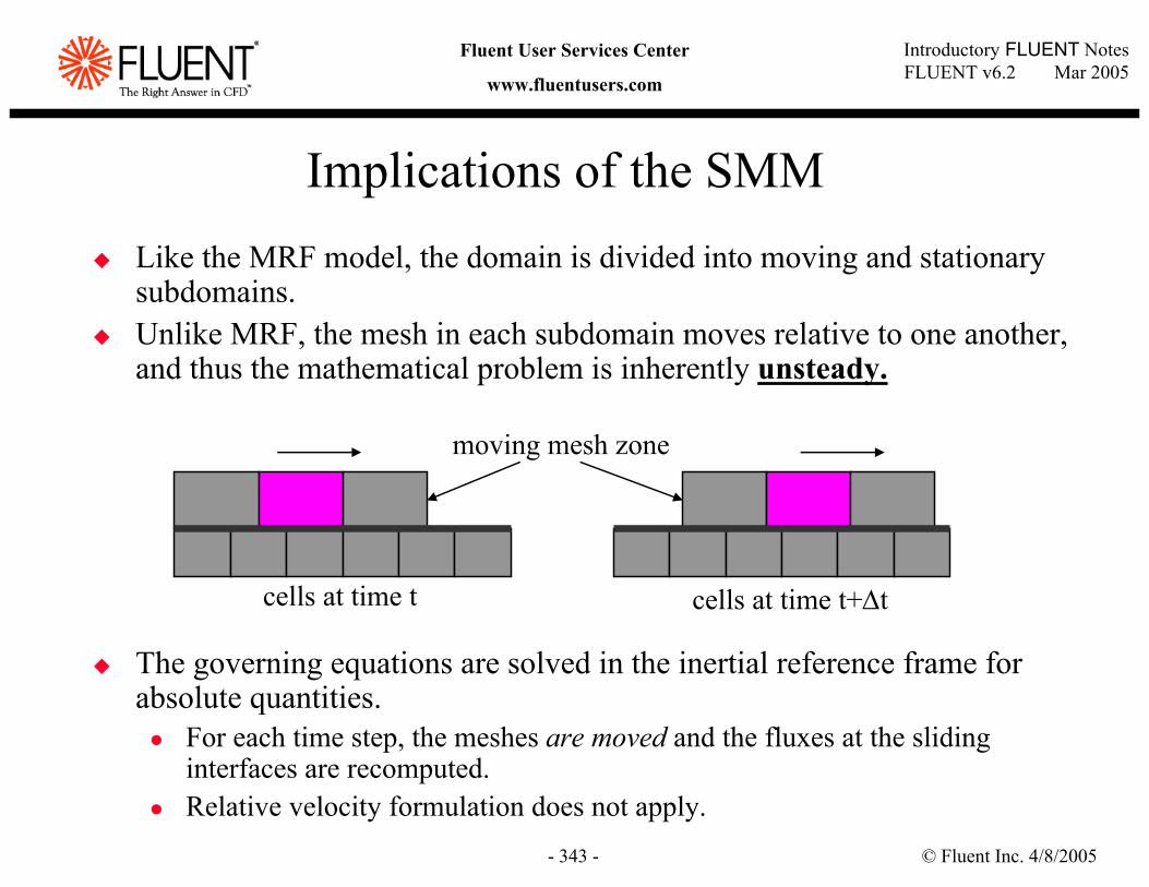
© Fluent Inc. 4/8/2005- 343 -



www.fluentusers.com

Implications of the SMMLike the MRF model, the domain is divided into moving and stationary subdomains.Unlike MRF, the mesh in each subdomain moves relative to one another, and thus the mathematical problem is inherently unsteady.

The governing equations are solved in the inertial reference frame for absolute quantities.

For each time step, the meshes are moved and the fluxes at the sliding interfaces are recomputed.Relative velocity formulation does not apply.

cells at time t cells at time t+∆t

moving mesh zone

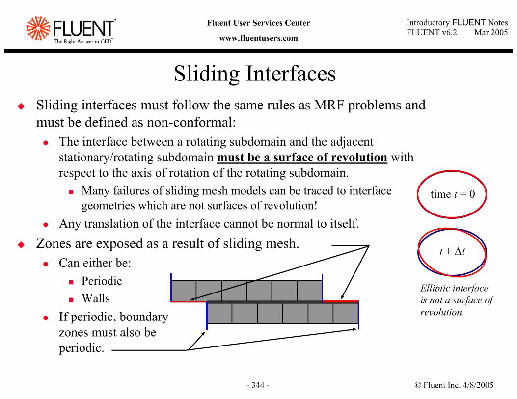
© Fluent Inc. 4/8/2005- 344 -



www.fluentusers.com

Sliding InterfacesSliding interfaces must follow the same rules as MRF problems and must be defined as non-conformal:

The interface between a rotating subdomain and the adjacent stationary/rotating subdomain must be a surface of revolution with respect to the axis of rotation of the rotating subdomain.

Many failures of sliding mesh models can be traced to interface geometries which are not surfaces of revolution!

Any translation of the interface cannot be normal to itself.Zones are exposed as a result of sliding mesh.

Can either be:PeriodicWalls

If periodic, boundaryzones must also beperiodic.

time t = 0

t + ∆t

Elliptic interface is not a surface of revolution.

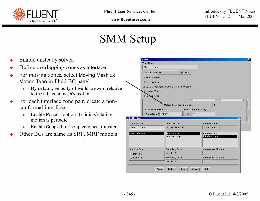
© Fluent Inc. 4/8/2005- 345 -



www.fluentusers.com

SMM Setup

Enable unsteady solver.Define overlapping zones as InterfaceFor moving zones, select Moving Mesh as Motion Type in Fluid BC panel.

By default, velocity of walls are zero relative to the adjacent mesh's motion.

For each interface zone pair, create a non-conformal interface

Enable Periodic option if sliding/rotating motion is periodic.Enable Coupled for conjugate heat transfer.

Other BCs are same as SRF, MRF models

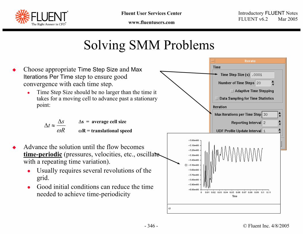
© Fluent Inc. 4/8/2005- 346 -



www.fluentusers.com

Solving SMM Problems

Choose appropriate Time Step Size and Max Iterations Per Time step to ensure good convergence with each time step.

Time Step Size should be no larger than the time it takes for a moving cell to advance past a stationary point:

Advance the solution until the flow becomes time-periodic (pressures, velocities, etc., oscillate with a repeating time variation).

Usually requires several revolutions of the grid.Good initial conditions can reduce the time needed to achieve time-periodicity

Rst

ω∆

≈∆∆s = average cell size

ωR = translational speed

© Fluent Inc. 4/8/2005- 347 -



www.fluentusers.com

Outline


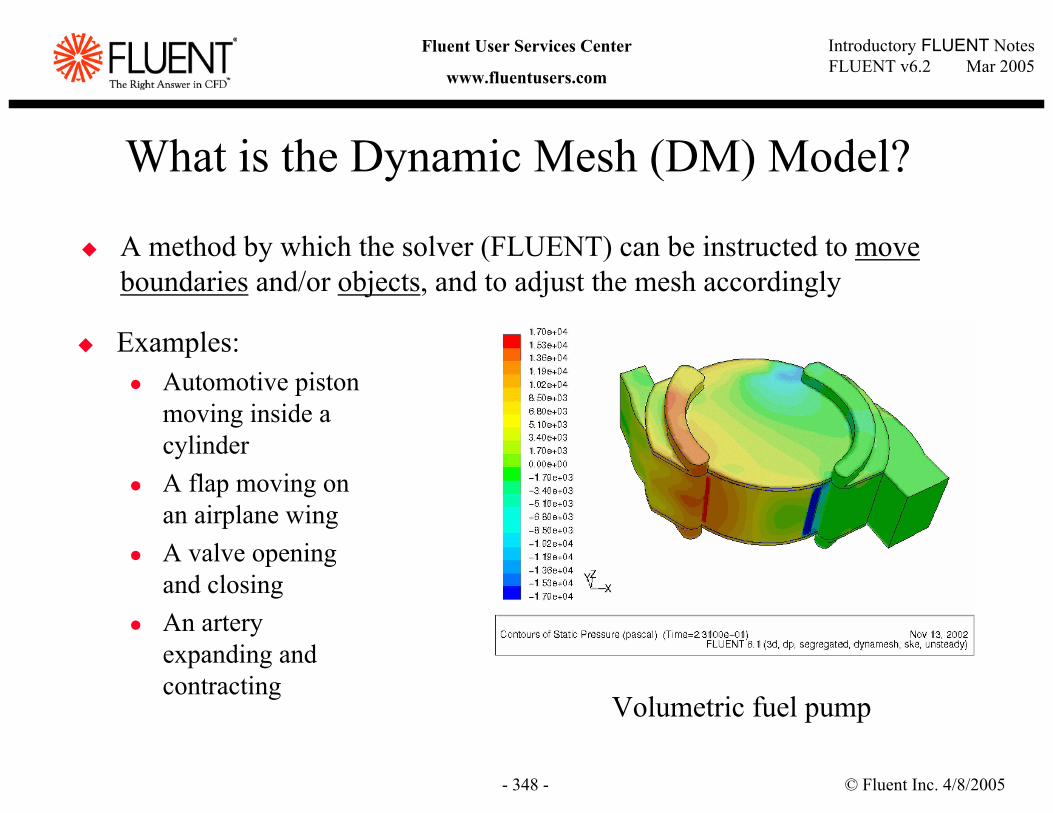
© Fluent Inc. 4/8/2005- 348 -



www.fluentusers.com

What is the Dynamic Mesh (DM) Model?

A method by which the solver (FLUENT) can be instructed to moveboundaries and/or objects, and to adjust the mesh accordingly

Examples:Automotive piston moving inside a cylinderA flap moving on an airplane wingA valve opening and closingAn artery expanding and contracting

Volumetric fuel pump

© Fluent Inc. 4/8/2005- 349 -



www.fluentusers.com

Dynamic Mesh (DM) Model: Features

Internal node positions are automatically calculated based on user specified boundary/object motion, cell type, and meshing schemes

Spring analogy (smoothing)Local remeshingLayering2.5 DUser defined mesh motion

Boundaries/Objects motion can be moved based on:In-cylinder motion (RPM, stroke length, crank angle, …)Prescribed motion via profiles or UDFCoupled motion based on hydrodynamic forces from the flow solution, via FLUENT’s 6 DOF model.

Different mesh motion schemes may be used for different zones. Connectivity between adjacent zones may be non-conformal.

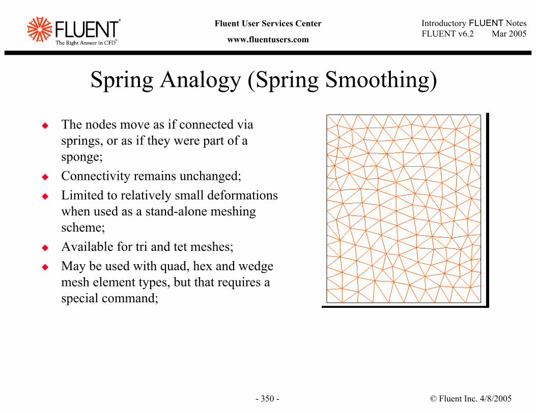
© Fluent Inc. 4/8/2005- 350 -



www.fluentusers.com

Spring Analogy (Spring Smoothing)

The nodes move as if connected via springs, or as if they were part of a sponge;Connectivity remains unchanged;Limited to relatively small deformations when used as a stand-alone meshing scheme;Available for tri and tet meshes;May be used with quad, hex and wedge mesh element types, but that requires a special command;

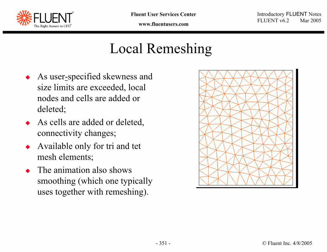
© Fluent Inc. 4/8/2005- 351 -



www.fluentusers.com

Local Remeshing

As user-specified skewness and size limits are exceeded, local nodes and cells are added or deleted;As cells are added or deleted, connectivity changes;Available only for tri and tet mesh elements;The animation also shows smoothing (which one typically uses together with remeshing).

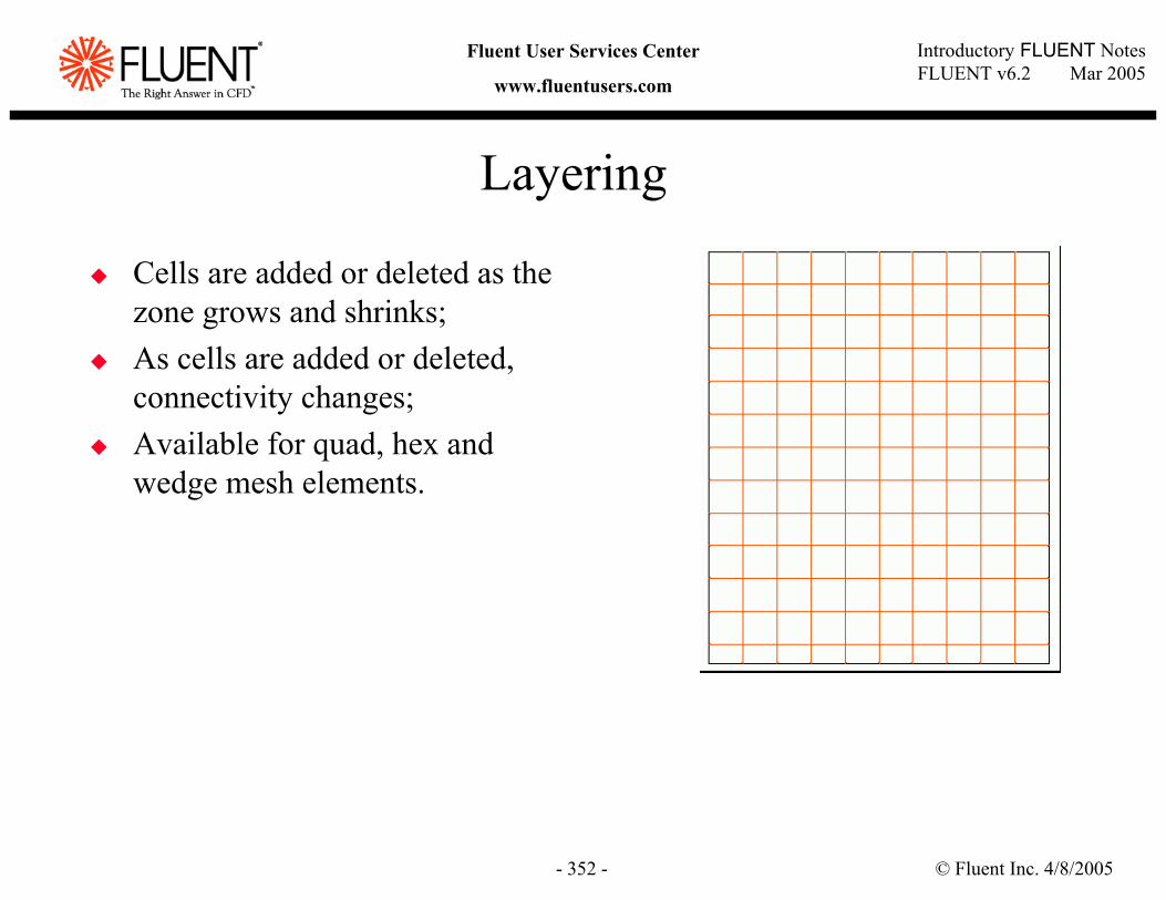
© Fluent Inc. 4/8/2005- 352 -



www.fluentusers.com

Layering

Cells are added or deleted as the zone grows and shrinks;As cells are added or deleted, connectivity changes;Available for quad, hex and wedge mesh elements.

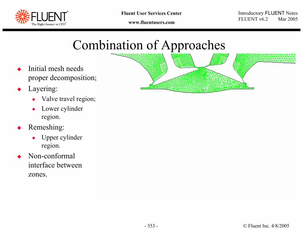
© Fluent Inc. 4/8/2005- 353 -



www.fluentusers.com

Combination of ApproachesInitial mesh needs proper decomposition;Layering:

Valve travel region; Lower cylinder region.

Remeshing: Upper cylinder region.

Non-conformal interface between zones.

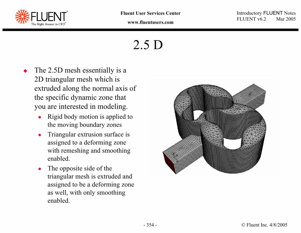
© Fluent Inc. 4/8/2005- 354 -



www.fluentusers.com

2.5 D

The 2.5D mesh essentially is a 2D triangular mesh which is extruded along the normal axis of the specific dynamic zone that you are interested in modeling.

Rigid body motion is applied to the moving boundary zonesTriangular extrusion surface is assigned to a deforming zone with remeshing and smoothing enabled. The opposite side of the triangular mesh is extruded and assigned to be a deforming zone as well, with only smoothing enabled.

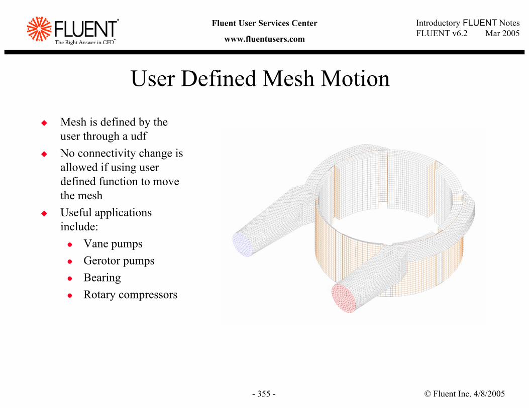
© Fluent Inc. 4/8/2005- 355 -



www.fluentusers.com

User Defined Mesh Motion

Mesh is defined by the user through a udfNo connectivity change is allowed if using user defined function to move the meshUseful applications include:

Vane pumpsGerotor pumpsBearingRotary compressors

© Fluent Inc. 4/8/2005- 356 -



www.fluentusers.com

6 DOF Coupled MotionObjects move as a result of aerodynamic forces and moments acting together with other forces, such as the gravity force, thrust forces, or ejector forces (i.e., forces used to initially push objects away from an airplane or rocket, to avoid collisions)In such cases, the motion and the flow field are thus coupled, and we call this coupled motionFluent provides a UDF (user-defined function) that computes the trajectory of an object based on the aerodynamic forces/moments,gravitational force, and ejector forces. This is often called a 6-DOF (degree-of-freedom) solver , and we refer to it as the 6-DOF UDF;The 6-DOF UDF is fully parallelized.

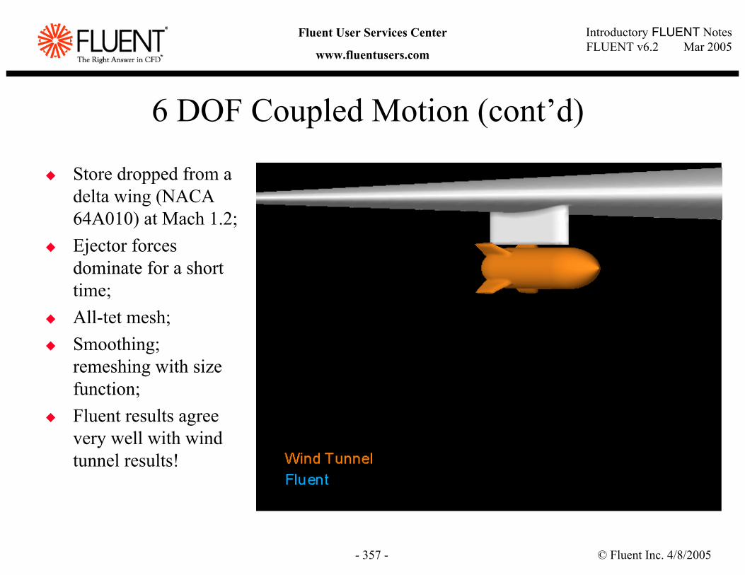
© Fluent Inc. 4/8/2005- 357 -



www.fluentusers.com

6 DOF Coupled Motion (cont’d)

Store dropped from a delta wing (NACA 64A010) at Mach 1.2;Ejector forces dominate for a short time;All-tet mesh;Smoothing; remeshing with size function;Fluent results agree very well with wind tunnel results!

© Fluent Inc. 4/8/2005- 358 -



www.fluentusers.com

Outline

Introduction and Overview of Modeling ApproachesSingle-Reference Frame (SRF) ModelMultiple Zones and Multiple-Reference Frame (MRF) ModelMixing Plane Model (MPM)Sliding Mesh Model (SMM)Dynamic (Moving and Deforming) Mesh ModelSummaryAppendix

© Fluent Inc. 4/8/2005- 359 -



www.fluentusers.com

SummaryFive different approaches may be used to model flows over movingparts.

Single (Rotating) Reference Frame ModelMultiple Reference Frame ModelMixing Plane ModelSliding Mesh ModelDynamic Mesh Model

Enabling these models, involves in part, changing the stationary fluid zones to either Moving Reference Frame or Moving Mesh.

Moving Mesh models must use unsteady solverLecture focused on rotating components, though, translational motion can also be addressed.

Restrictions on geometry of interface still applies.SMM can be used, for example, to study flow between two trains passing each other.

© Fluent Inc. 4/8/2005- 360 -



www.fluentusers.com

Appendix

Navier-Stokes equations for moving reference framesRelative Velocity FormulationAbsolution Velocity Formulation

Navier-Stokes equations for sliding mesh problems

© Fluent Inc. 4/8/2005- 361 -



www.fluentusers.com

N-S Equations: Rotating Reference FrameTwo different formulations are used in Fluent

Relative Velocity Formulation (RVF)Obtained by transforming the stationary frame N-S equations to a rotating reference frameUses the relative velocity as the dependent variable in the momentum equationsUses the relative total internal energy as the dependent variable in the energy equation

Absolute Velocity Formulation (AVF)Derived from the relative velocity formulationUses the absolute velocity as the dependent variable in the momentum equationsUses the absolute total internal energy as the dependent variable in the energy equation

NOTE: RVF and AVF are equivalent forms of the N-S equations!Identical solutions should be obtained from either formulation with equivalent boundary conditions

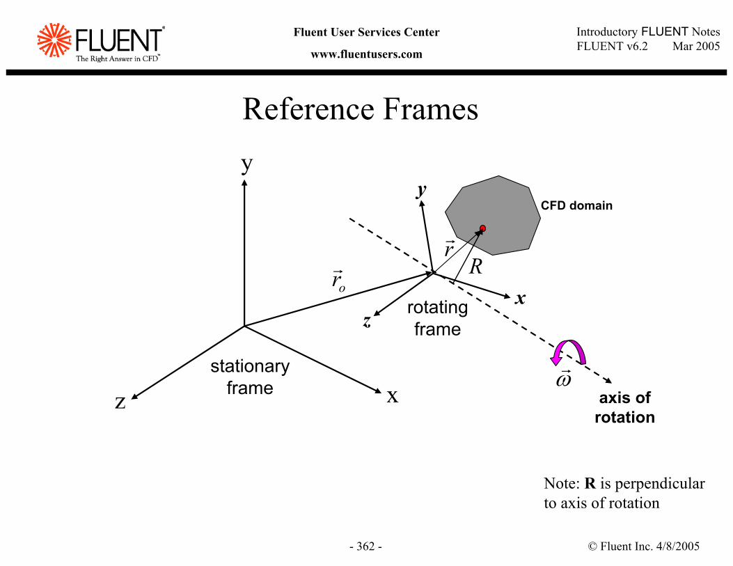
© Fluent Inc. 4/8/2005- 362 -



www.fluentusers.com

Reference Frames

x

y

z

z

y

x

stationaryframe

rotatingframe

axis ofrotation

rr

ωr

CFD domain

orr R

Note: R is perpendicularto axis of rotation

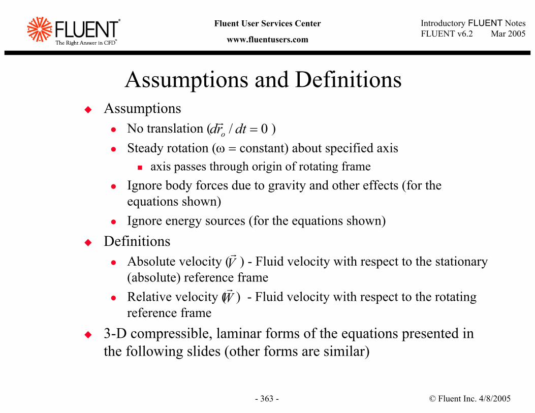
© Fluent Inc. 4/8/2005- 363 -



www.fluentusers.com

AssumptionsNo translation ( )Steady rotation (ω = constant) about specified axis

axis passes through origin of rotating frameIgnore body forces due to gravity and other effects (for the equations shown)Ignore energy sources (for the equations shown)

DefinitionsAbsolute velocity ( ) - Fluid velocity with respect to the stationary (absolute) reference frameRelative velocity ( ) - Fluid velocity with respect to the rotating reference frame

3-D compressible, laminar forms of the equations presented in the following slides (other forms are similar)

Assumptions and Definitions

Vr

Wr

0/ =dtrd or

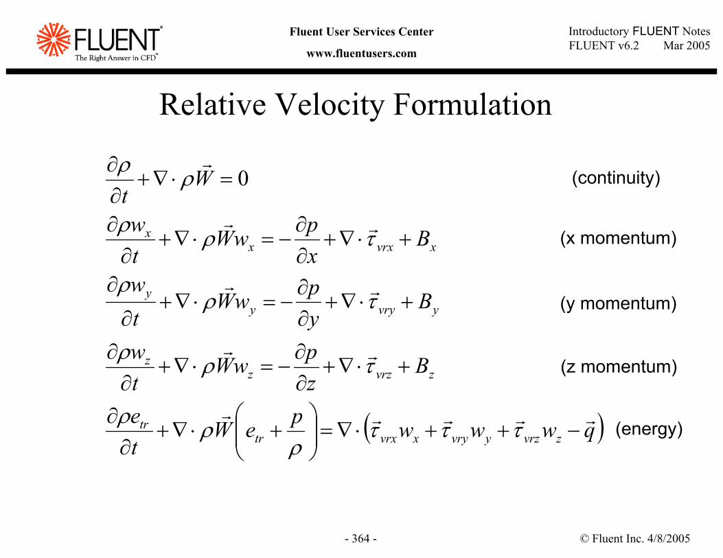
© Fluent Inc. 4/8/2005- 364 -



www.fluentusers.com

Relative Velocity Formulation

( )qwwwpeWte

BzpwW

tw

BypwW

tw

BxpwW

tw

Wt

zvrzyvryxvrxtrtr

zvrzzz

yvryyy

xvrxxx

rrrrr

rr

rr

rr

r

−++⋅∇=

+⋅∇+

∂∂

+⋅∇+∂∂

−=⋅∇+∂

∂

+⋅∇+∂∂

−=⋅∇+∂

∂

+⋅∇+∂∂

−=⋅∇+∂

∂

=⋅∇+∂∂

τττρ

ρρ

τρρ

τρρ

τρρ

ρρ 0 (continuity)

(x momentum)

(y momentum)

(z momentum)

(energy)

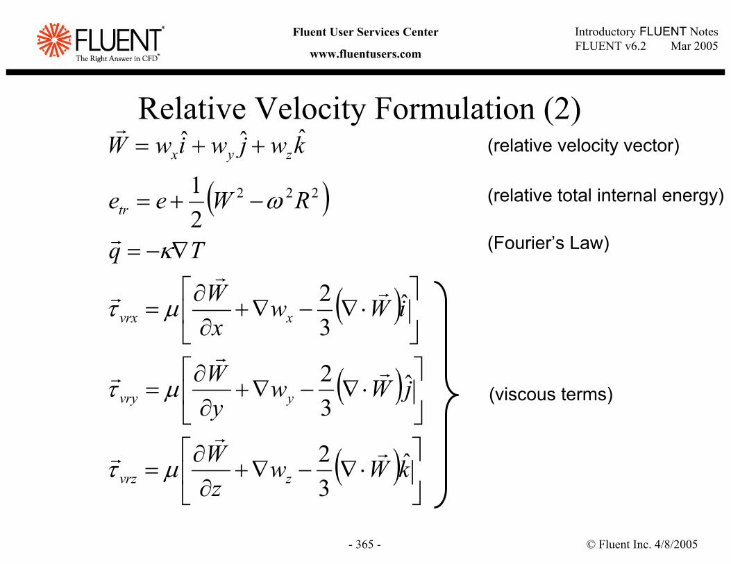
© Fluent Inc. 4/8/2005- 365 -



www.fluentusers.com

Relative Velocity Formulation (2)

( )

( )

( )

( )

⋅∇−∇+

∂∂

=

⋅∇−∇+

∂∂

=

⋅∇−∇+

∂∂

=

∇−=

−+=

++=

kWwz

W

jWwy

W

iWwx

W

Tq

RWee

kwjwiwW

zvrz

yvry

xvrx

tr

zyx

ˆ32

ˆ32

ˆ32

21

ˆˆˆ

222

rr

r

rr

r

rr

r

r

r

µτ

µτ

µτ

κ

ω

(relative velocity vector)

(relative total internal energy)

(Fourier’s Law)

(viscous terms)

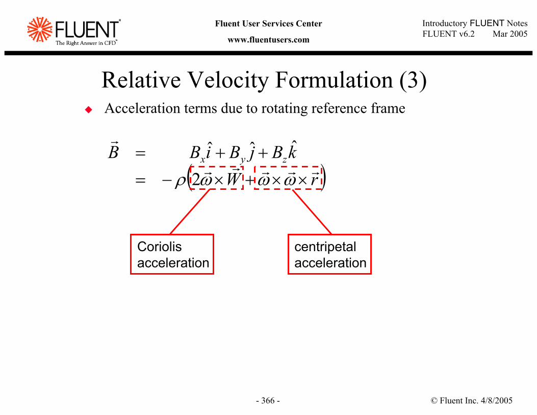
© Fluent Inc. 4/8/2005- 366 -



www.fluentusers.com

Relative Velocity Formulation (3)Acceleration terms due to rotating reference frame

( )rWkBjBiBB zyx

rrrrr

r

××+×−=++=

ωωωρ 2

ˆˆˆ

Coriolisacceleration

centripetalacceleration

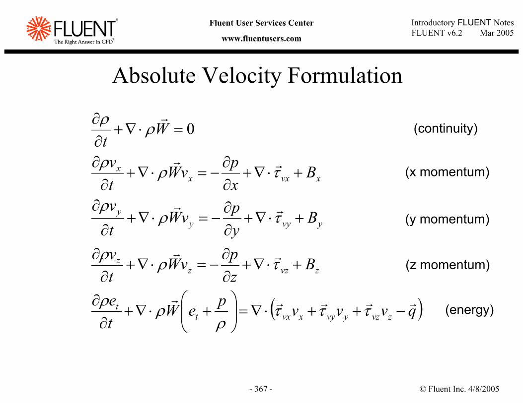
© Fluent Inc. 4/8/2005- 367 -



www.fluentusers.com

Absolute Velocity Formulation

( )qvvvpeWte

BzpvW

tv

BypvW

tv

BxpvW

tv

Wt

zvzyvyxvxtt

zvzzz

yvyyy

xvxxx

rrrrr

rr

rr

rr

r

−++⋅∇=

+⋅∇+

∂∂

+⋅∇+∂∂

−=⋅∇+∂

∂

+⋅∇+∂∂

−=⋅∇+∂

∂

+⋅∇+∂∂

−=⋅∇+∂

∂

=⋅∇+∂∂

τττρ

ρρ

τρρ

τρρ

τρρ

ρρ 0 (continuity)

(x momentum)

(y momentum)

(z momentum)

(energy)

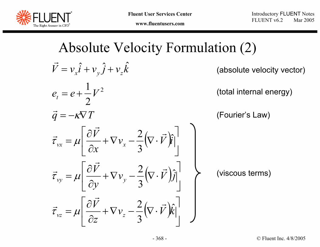
© Fluent Inc. 4/8/2005- 368 -



www.fluentusers.com

Absolute Velocity Formulation (2)

( )

( )

( )

⋅∇−∇+

∂∂

=

⋅∇−∇+

∂∂

=

⋅∇−∇+

∂∂

=

∇−=

+=

++=

kVvzV

jVvyV

iVvxV

Tq

Vee

kvjvivV

zvz

yvy

xvx

t

zyx

ˆ32

ˆ32

ˆ32

21

ˆˆˆ

2

rr

r

rr

r

rr

r

r

r

µτ

µτ

µτ

κ

(absolute velocity vector)

(total internal energy)

(Fourier’s Law)

(viscous terms)

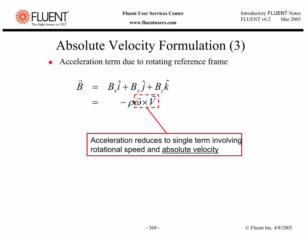
© Fluent Inc. 4/8/2005- 369 -



www.fluentusers.com

Absolute Velocity Formulation (3)Acceleration term due to rotating reference frame

VkBjBiBB zyx rr

r

×−=++=

ωρ

ˆˆˆ

Acceleration reduces to single term involvingrotational speed and absolute velocity

© Fluent Inc. 4/8/2005- 370 -



www.fluentusers.com

Velocity Formulation RecommendationsUse AVF when inflow comes from a stationary domain

Absolute total pressure or absolute velocities are usually known in this caseExample: Flow in a ducted fan system, where inlet is a stationary duct

Use RVF with closed domains (all surfaces are moving) or if inflow comes from a rotating domain

Relative total pressure or relative velocities are usually known in this caseExample: Swirling flow in a disk cavity

As noted previously, RVF and AVF are equivalent, and therefore either can be used successfully for most problems

Discrepancies on the same mesh can occur if the magnitude of absolute velocity gradients are very different than magnitude of the relative velocity gradientsDifferences between solutions should disappear with suitable mesh refinement

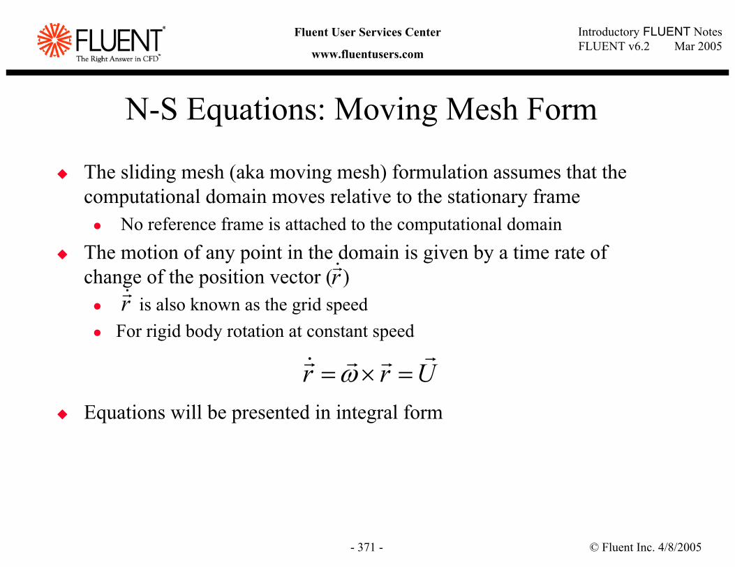
© Fluent Inc. 4/8/2005- 371 -



www.fluentusers.com

N-S Equations: Moving Mesh Form

The sliding mesh (aka moving mesh) formulation assumes that the computational domain moves relative to the stationary frame

No reference frame is attached to the computational domain The motion of any point in the domain is given by a time rate ofchange of the position vector ( )

is also known as the grid speedFor rigid body rotation at constant speed

Equations will be presented in integral form

r&r

r&r

Urrrrr&r =×= ω

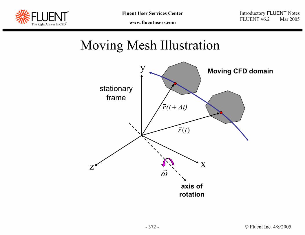
© Fluent Inc. 4/8/2005- 372 -



www.fluentusers.com

Moving Mesh Illustration

x

y

z

stationaryframe

axis ofrotation

∆t)(tr +r

ωr

Moving CFD domain

)(trr

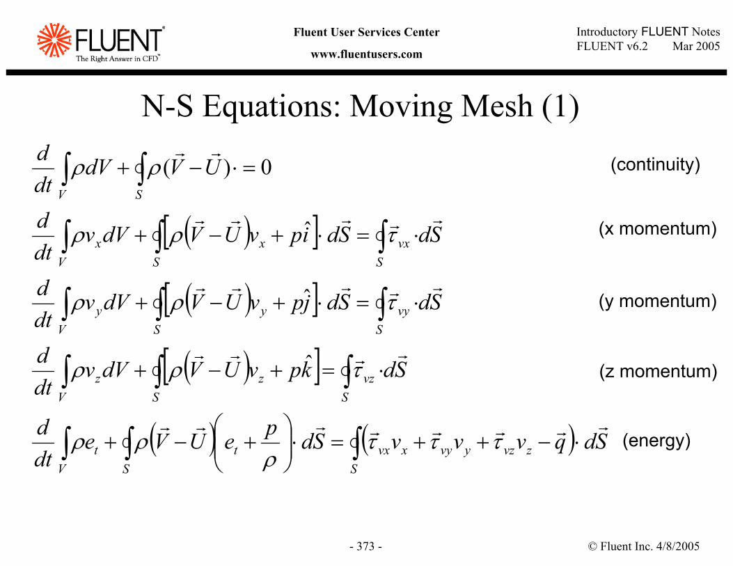
© Fluent Inc. 4/8/2005- 373 -



www.fluentusers.com

N-S Equations: Moving Mesh (1)

( )[ ]

( )[ ]

( )[ ]

( ) ( ) SdqvvvSdpeUVedtd

SdkpvUVdVvdtd

SdSdjpvUVdVvdtd

SdSdipvUVdVvdtd

UVdVdtd

Szvzyvyxvx

St

Vt

Svz

Sz

Vz

Svy

Sy

Vy

Svx

Sx

Vx

SV

rrrrrrrr

rrrr

rrrrr

rrrrr

rr

⋅−++=⋅

+−+

⋅=+−+

⋅=⋅+−+

⋅=⋅+−+

=⋅−+

∫∫∫

∫∫∫

∫∫∫

∫∫∫

∫∫

τττρ

ρρ

τρρ

τρρ

τρρ

ρρ

ˆ

ˆ

ˆ

0)( (continuity)

(x momentum)

(y momentum)

(z momentum)

(energy)

© Fluent Inc. 4/8/2005- 374 -



www.fluentusers.com

N-S Equations: Moving Mesh (2)

In the foregoing equations, V and are the volume and boundarysurface of the control volume, respectively

V remains constant since the mesh is not deforming= since the area vectors are changing orientation as control volume

movesThe time derivative ( ) represents differentiation with respect to time following the moving domainThe convecting velocity is again the relative velocity

All spatial derivatives computed relative to the stationary frame

dtd /

Sr

)(tSr

Sr

Documents

Fluent 6.2 Software Capabilities - Freevincent.chapin.free.fr/Cours CFD/Doc/Fluent-v6.2-lect_all.pdf · Fluent 6.2 applications: zExternal/internal automotive flows and in-cylinder