Embed Size (px)
Citation preview

FLUENT 6.2 UDF Manual
January 2005

Copyright c© 2005 by Fluent Inc.All rights reserved. No part of this document may be reproduced or otherwise used in
any form without express written permission from Fluent Inc.
Airpak, FIDAP, FLUENT, FloWizard, GAMBIT, Icemax, Icepak, Icepro, MixSim, andPOLYFLOW are registered trademarks of Fluent Inc. All other products or name
brands are trademarks of their respective holders.
CHEMKIN is a registered trademark of Reaction Design Inc.
Portions of this program include material copyrighted by PathScale Corporation2003-2004.
Fluent Inc.Centerra Resource Park
10 Cavendish CourtLebanon, NH 03766

About This Document
User-defined functions (UDFs) allow you to customize FLUENT and can significantlyenhance its capabilities. This UDF Manual presents detailed information on how towrite, compile, and use UDFs in FLUENT. Examples have also been included, whereavailable.
Information in this manual is presented in the following chapters:
• Chapter 1: Overview
• Chapter 2: C Programming Basics for UDFs
• Chapter 3: A Step-by-Step UDF Example
• Chapter 4: Defining a UDF Using a DEFINE Macro
• Chapter 5: Macros for Accessing FLUENT Solver Variables
• Chapter 6: UDF Utilities
• Chapter 7: Interpreting UDF Source Files
• Chapter 8: Compiling UDF Source Files
• Chapter 9: Hooking Your UDF to FLUENT
• Chapter 10: Parallel UDF Usage
• Chapter 11: User-Defined Scalar (UDS) Transport Modeling
• Chapter 12: Sample Problems
This document provides some basic information about the C programming languageas it relates to UDFs in FLUENT and assumes that you have some programming ex-perience with C. If you are unfamiliar with C, please consult a C language reference(e.g., [2]) for basic information.
This document does not imply responsibility on the part of Fluent Inc. for the ac-curacy or stability of solutions obtained using UDFs that are either user-generatedor provided by Fluent Inc. Support for current license holders will be limited toguidance related to communication between a UDF and the FLUENT solver. Otheraspects of the UDF development process that include conceptual function design,implementation (writing C code), compilation and debugging of C source code, ex-ecution of the UDF, and function design verification will remain the responsibilityof the UDF author.
c© Fluent Inc. January 11, 2005 i

About This Document
ii c© Fluent Inc. January 11, 2005

Contents
1 Overview 1-1
1.1 What is a User-Defined Function (UDF)? . . . . . . . . . . . . . . . . . 1-1
1.2 Why Use UDFs? . . . . . . . . . . . . . . . . . . . . . . . . . . . . . . . 1-3
1.3 Limitations . . . . . . . . . . . . . . . . . . . . . . . . . . . . . . . . . . 1-3
1.4 Writing UDFs . . . . . . . . . . . . . . . . . . . . . . . . . . . . . . . . . 1-4
1.5 Defining Your UDF Using DEFINE Macros . . . . . . . . . . . . . . . . . 1-4
1.5.1 Including the udf.h Header File in Your Source File . . . . . . . 1-5
1.6 Interpreting or Compiling UDFs . . . . . . . . . . . . . . . . . . . . . . 1-6
1.6.1 Differences Between Interpreted and Compiled UDFs . . . . . . . 1-7
1.7 Hooking UDFs to Your FLUENT Model . . . . . . . . . . . . . . . . . . 1-8
1.8 Grid Terminology . . . . . . . . . . . . . . . . . . . . . . . . . . . . . . . 1-8
1.9 Data Types in FLUENT . . . . . . . . . . . . . . . . . . . . . . . . . . . 1-10
1.10 Calling Sequence of a UDF in the FLUENT Solution Process . . . . . . . 1-12
1.11 Special Considerations for Multiphase UDFs . . . . . . . . . . . . . . . . 1-15
1.11.1 Multiphase-specific Data Types . . . . . . . . . . . . . . . . . . . 1-15
2 C Programming Basics for UDFs 2-1
2.1 Introduction . . . . . . . . . . . . . . . . . . . . . . . . . . . . . . . . . 2-1
2.2 Commenting Your C Code . . . . . . . . . . . . . . . . . . . . . . . . . . 2-2
2.3 C Data Types in FLUENT . . . . . . . . . . . . . . . . . . . . . . . . . . 2-2
2.4 Constants . . . . . . . . . . . . . . . . . . . . . . . . . . . . . . . . . . . 2-3
2.5 Variables . . . . . . . . . . . . . . . . . . . . . . . . . . . . . . . . . . . 2-3
2.5.1 Declaring Variables . . . . . . . . . . . . . . . . . . . . . . . . . 2-4
2.5.2 External Variables . . . . . . . . . . . . . . . . . . . . . . . . . . 2-5
2.5.3 Static Variables . . . . . . . . . . . . . . . . . . . . . . . . . . . 2-7
c© Fluent Inc. January 11, 2005 i

CONTENTS
2.6 User-Defined Data Types . . . . . . . . . . . . . . . . . . . . . . . . . . 2-8
2.7 Casting . . . . . . . . . . . . . . . . . . . . . . . . . . . . . . . . . . . . 2-8
2.8 Functions . . . . . . . . . . . . . . . . . . . . . . . . . . . . . . . . . . . 2-8
2.9 Arrays . . . . . . . . . . . . . . . . . . . . . . . . . . . . . . . . . . . . . 2-9
2.10 Pointers . . . . . . . . . . . . . . . . . . . . . . . . . . . . . . . . . . . . 2-9
2.11 Control Statements . . . . . . . . . . . . . . . . . . . . . . . . . . . . . . 2-11
2.11.1 if Statement . . . . . . . . . . . . . . . . . . . . . . . . . . . . . 2-11
2.11.2 if-else Statement . . . . . . . . . . . . . . . . . . . . . . . . . 2-11
2.11.3 for Loops . . . . . . . . . . . . . . . . . . . . . . . . . . . . . . 2-12
2.12 Common C Operators . . . . . . . . . . . . . . . . . . . . . . . . . . . . 2-13
2.12.1 Arithmetic Operators . . . . . . . . . . . . . . . . . . . . . . . . 2-13
2.12.2 Logical Operators . . . . . . . . . . . . . . . . . . . . . . . . . . 2-13
2.13 C Library Functions . . . . . . . . . . . . . . . . . . . . . . . . . . . . . 2-14
2.13.1 Trigonometric Functions . . . . . . . . . . . . . . . . . . . . . . . 2-14
2.13.2 Miscellaneous Mathematical Functions . . . . . . . . . . . . . . . 2-14
2.13.3 Standard I/O Functions . . . . . . . . . . . . . . . . . . . . . . . 2-15
2.14 Preprocessor Directives . . . . . . . . . . . . . . . . . . . . . . . . . . . 2-18
2.15 Comparison with FORTRAN . . . . . . . . . . . . . . . . . . . . . . . . 2-19
3 A Step-by-Step UDF Example 3-1
3.1 Process Overview . . . . . . . . . . . . . . . . . . . . . . . . . . . . . . . 3-1
3.1.1 Step 1: Define Your Problem . . . . . . . . . . . . . . . . . . . . 3-2
3.1.2 Step 2: Create a C Source File . . . . . . . . . . . . . . . . . . . 3-4
3.1.3 Step 3: Start FLUENT and Read (or Set Up) the Case File . . . 3-5
3.1.4 Step 4: Interpret or Compile the Source File . . . . . . . . . . . 3-5
3.1.5 Step 5: Hook Your UDF to FLUENT . . . . . . . . . . . . . . . . 3-12
3.1.6 Step 6: Run the Calculation . . . . . . . . . . . . . . . . . . . . 3-12
3.1.7 Step 7: Analyze the Numerical Solution and Compare toExpected Results . . . . . . . . . . . . . . . . . . . . . . . . . . 3-13
ii c© Fluent Inc. January 11, 2005

CONTENTS
4 Defining a UDF Using a DEFINE Macro 4-1
4.1 Introduction . . . . . . . . . . . . . . . . . . . . . . . . . . . . . . . . . 4-1
4.2 Model-Independent DEFINE Macros . . . . . . . . . . . . . . . . . . . . . 4-2
4.2.1 DEFINE ADJUST . . . . . . . . . . . . . . . . . . . . . . . . . . . . 4-4
4.2.2 DEFINE EXECUTE AT END . . . . . . . . . . . . . . . . . . . . . . . 4-7
4.2.3 DEFINE EXECUTE FROM GUI . . . . . . . . . . . . . . . . . . . . . 4-10
4.2.4 DEFINE EXECUTE ON LOADING . . . . . . . . . . . . . . . . . . . . 4-13
4.2.5 DEFINE INIT . . . . . . . . . . . . . . . . . . . . . . . . . . . . . 4-17
4.2.6 DEFINE ON DEMAND . . . . . . . . . . . . . . . . . . . . . . . . . . 4-20
4.2.7 DEFINE RW FILE . . . . . . . . . . . . . . . . . . . . . . . . . . . 4-23
4.3 Model-Dependent DEFINE Macros . . . . . . . . . . . . . . . . . . . . . . 4-26
4.3.1 DEFINE CHEM STEP . . . . . . . . . . . . . . . . . . . . . . . . . . 4-34
4.3.2 DEFINE DELTAT . . . . . . . . . . . . . . . . . . . . . . . . . . . . 4-36
4.3.3 DEFINE DIFFUSIVITY . . . . . . . . . . . . . . . . . . . . . . . . 4-38
4.3.4 DEFINE DOM DIFFUSE REFLECTIVITY . . . . . . . . . . . . . . . . 4-40
4.3.5 DEFINE DOM SOURCE . . . . . . . . . . . . . . . . . . . . . . . . . 4-42
4.3.6 DEFINE DOM SPECULAR REFLECTIVITY . . . . . . . . . . . . . . . 4-44
4.3.7 DEFINE GRAY BAND ABS COEFF . . . . . . . . . . . . . . . . . . . . 4-46
4.3.8 DEFINE HEAT FLUX . . . . . . . . . . . . . . . . . . . . . . . . . . 4-48
4.3.9 DEFINE NET REACTION RATE . . . . . . . . . . . . . . . . . . . . . 4-50
4.3.10 DEFINE NOX RATE . . . . . . . . . . . . . . . . . . . . . . . . . . 4-52
4.3.11 DEFINE PR RATE . . . . . . . . . . . . . . . . . . . . . . . . . . . 4-55
4.3.12 DEFINE PRANDTL . . . . . . . . . . . . . . . . . . . . . . . . . . . 4-61
4.3.13 DEFINE PROFILE . . . . . . . . . . . . . . . . . . . . . . . . . . . 4-71
4.3.14 DEFINE PROPERTY . . . . . . . . . . . . . . . . . . . . . . . . . . 4-84
4.3.15 DEFINE SCAT PHASE FUNC . . . . . . . . . . . . . . . . . . . . . . 4-93
4.3.16 DEFINE SOLAR INTENSITY . . . . . . . . . . . . . . . . . . . . . . 4-96
4.3.17 DEFINE SOURCE . . . . . . . . . . . . . . . . . . . . . . . . . . . . 4-98
4.3.18 DEFINE SR RATE . . . . . . . . . . . . . . . . . . . . . . . . . . . 4-102
c© Fluent Inc. January 11, 2005 iii

CONTENTS
4.3.19 DEFINE TURB PREMIX SOURCE . . . . . . . . . . . . . . . . . . . . 4-109
4.3.20 DEFINE TURBULENT VISCOSITY . . . . . . . . . . . . . . . . . . . 4-112
4.3.21 DEFINE UDS FLUX . . . . . . . . . . . . . . . . . . . . . . . . . . 4-116
4.3.22 DEFINE UDS UNSTEADY . . . . . . . . . . . . . . . . . . . . . . . . 4-120
4.3.23 DEFINE VR RATE . . . . . . . . . . . . . . . . . . . . . . . . . . . 4-122
4.4 Multiphase DEFINE Macros . . . . . . . . . . . . . . . . . . . . . . . . . 4-126
4.4.1 DEFINE CAVITATION RATE . . . . . . . . . . . . . . . . . . . . . . 4-128
4.4.2 DEFINE EXCHANGE PROPERTY . . . . . . . . . . . . . . . . . . . . 4-131
4.4.3 DEFINE HET RXN RATE . . . . . . . . . . . . . . . . . . . . . . . . 4-137
4.4.4 DEFINE MASS TRANSFER . . . . . . . . . . . . . . . . . . . . . . . 4-141
4.4.5 DEFINE VECTOR EXCHANGE PROPERTY . . . . . . . . . . . . . . . . 4-144
4.5 Dynamic Mesh DEFINE Macros . . . . . . . . . . . . . . . . . . . . . . . 4-147
4.5.1 DEFINE CG MOTION . . . . . . . . . . . . . . . . . . . . . . . . . . 4-148
4.5.2 DEFINE GEOM . . . . . . . . . . . . . . . . . . . . . . . . . . . . . 4-151
4.5.3 DEFINE GRID MOTION . . . . . . . . . . . . . . . . . . . . . . . . 4-153
4.5.4 DEFINE SDOF PROPERTIES . . . . . . . . . . . . . . . . . . . . . . 4-156
4.6 DPM DEFINE Macros . . . . . . . . . . . . . . . . . . . . . . . . . . . . . 4-161
4.6.1 DEFINE DPM BC . . . . . . . . . . . . . . . . . . . . . . . . . . . . 4-163
4.6.2 DEFINE DPM BODY FORCE . . . . . . . . . . . . . . . . . . . . . . . 4-171
4.6.3 DEFINE DPM DRAG . . . . . . . . . . . . . . . . . . . . . . . . . . 4-173
4.6.4 DEFINE DPM EROSION . . . . . . . . . . . . . . . . . . . . . . . . 4-175
4.6.5 DEFINE DPM INJECTION INIT . . . . . . . . . . . . . . . . . . . . 4-181
4.6.6 DEFINE DPM LAW . . . . . . . . . . . . . . . . . . . . . . . . . . . 4-185
4.6.7 DEFINE DPM OUTPUT . . . . . . . . . . . . . . . . . . . . . . . . . 4-187
4.6.8 DEFINE DPM PROPERTY . . . . . . . . . . . . . . . . . . . . . . . . 4-189
4.6.9 DEFINE DPM SCALAR UPDATE . . . . . . . . . . . . . . . . . . . . . 4-193
4.6.10 DEFINE DPM SOURCE . . . . . . . . . . . . . . . . . . . . . . . . . 4-197
4.6.11 DEFINE DPM SPRAY COLLIDE . . . . . . . . . . . . . . . . . . . . . 4-199
iv c© Fluent Inc. January 11, 2005

CONTENTS
4.6.12 DEFINE DPM SWITCH . . . . . . . . . . . . . . . . . . . . . . . . . 4-202
4.6.13 DEFINE DPM TIMESTEP . . . . . . . . . . . . . . . . . . . . . . . . 4-208
5 Macros for Accessing FLUENT Solver Variables 5-1
5.1 Introduction . . . . . . . . . . . . . . . . . . . . . . . . . . . . . . . . . 5-2
5.2 Grid Variables . . . . . . . . . . . . . . . . . . . . . . . . . . . . . . . . 5-4
5.2.1 Node Definitions . . . . . . . . . . . . . . . . . . . . . . . . . . . 5-4
5.2.2 Face Definitions . . . . . . . . . . . . . . . . . . . . . . . . . . . 5-4
5.2.3 Cell Definitions . . . . . . . . . . . . . . . . . . . . . . . . . . . . 5-6
5.2.4 Connectivity Variables . . . . . . . . . . . . . . . . . . . . . . . . 5-11
5.3 Cell Variables . . . . . . . . . . . . . . . . . . . . . . . . . . . . . . . . . 5-11
5.3.1 Flow Variable Macros . . . . . . . . . . . . . . . . . . . . . . . . 5-11
5.3.2 Material Property Macros . . . . . . . . . . . . . . . . . . . . . . 5-17
5.3.3 Reynolds Stress Model Macros . . . . . . . . . . . . . . . . . . . 5-20
5.4 Face Variables . . . . . . . . . . . . . . . . . . . . . . . . . . . . . . . . 5-20
5.4.1 Flow Variable Macros at a Boundary Face . . . . . . . . . . . . . 5-20
5.4.2 Flow Variable Macros at Interior and Boundary Faces . . . . . . 5-20
5.5 User-Defined Scalar (UDS) Variables . . . . . . . . . . . . . . . . . . . . 5-22
5.5.1 Accessing UDS Face Variables With F UDSI . . . . . . . . . . . . 5-22
5.5.2 Accessing UDS Cell Variables With C UDSI . . . . . . . . . . . . 5-22
5.5.3 Reserving UDS Variables . . . . . . . . . . . . . . . . . . . . . . 5-22
5.5.4 Unreserving UDS Variables . . . . . . . . . . . . . . . . . . . . . 5-23
5.5.5 Setting UDS Variable Names . . . . . . . . . . . . . . . . . . . . 5-24
5.6 User-Defined Memory (UDM) Variables . . . . . . . . . . . . . . . . . . 5-24
5.6.1 F UDMI for Storing or Accessing UDM Face Values . . . . . . . . 5-24
5.6.2 C UDMI for Storing or Accessing UDS Cell Values . . . . . . . . . 5-25
5.6.3 Example UDF that Utilizes UDM and UDS Variables . . . . . . 5-25
5.6.4 Reserving UDM Variables for a UDF Library . . . . . . . . . . . 5-27
5.6.5 Unreserving UDM variables . . . . . . . . . . . . . . . . . . . . . 5-32
c© Fluent Inc. January 11, 2005 v
CONTENTS
5.6.6 Setting UDM Variable Names . . . . . . . . . . . . . . . . . . . . 5-32
5.7 Multiphase Variables . . . . . . . . . . . . . . . . . . . . . . . . . . . . . 5-32
5.8 Dynamic Mesh Variables . . . . . . . . . . . . . . . . . . . . . . . . . . . 5-33
5.9 DPM Variables . . . . . . . . . . . . . . . . . . . . . . . . . . . . . . . . 5-33
5.10 NOx Variables . . . . . . . . . . . . . . . . . . . . . . . . . . . . . . . . 5-39
6 UDF Utilities 6-1
6.1 Introduction . . . . . . . . . . . . . . . . . . . . . . . . . . . . . . . . . 6-1
6.2 Looping Macros . . . . . . . . . . . . . . . . . . . . . . . . . . . . . . . . 6-2
6.3 Multiphase-Specific Looping Macros . . . . . . . . . . . . . . . . . . . . 6-7
6.4 Setting Face Variables Using F PROFILE . . . . . . . . . . . . . . . . . . 6-12
6.5 Accessing Variables That Are Not Passed as Arguments . . . . . . . . . 6-13
6.5.1 Domain Pointer Using Get Domain . . . . . . . . . . . . . . . . . 6-14
6.5.2 Phase Domain Pointer Using DOMAIN SUB DOMAIN . . . . . . . . . 6-16
6.5.3 Phase-Level Thread Pointer Using THREAD SUB THREAD . . . . . . 6-17
6.5.4 Phase Thread Pointer Array Using THREAD SUB THREADS . . . . . 6-18
6.5.5 Mixture Domain Pointer Using DOMAIN SUPER DOMAIN . . . . . . 6-19
6.5.6 Mixture Thread Pointer Using THREAD SUPER THREAD . . . . . . 6-19
6.5.7 Thread Pointer Using Lookup Thread . . . . . . . . . . . . . . . 6-20
6.5.8 Zone ID Using THREAD ID . . . . . . . . . . . . . . . . . . . . . . 6-21
6.5.9 DOMAIN ID . . . . . . . . . . . . . . . . . . . . . . . . . . . . . . 6-22
6.5.10 PHASE DOMAIN INDEX . . . . . . . . . . . . . . . . . . . . . . . . 6-22
6.6 Vector and Dimension Macros . . . . . . . . . . . . . . . . . . . . . . . . 6-22
6.6.1 Macros for Dealing with Two and Three Dimensions . . . . . . . 6-23
6.6.2 Vector Operations . . . . . . . . . . . . . . . . . . . . . . . . . . 6-25
6.7 Time-Dependent Macros . . . . . . . . . . . . . . . . . . . . . . . . . . . 6-28
6.8 User-Defined Scheme Variables . . . . . . . . . . . . . . . . . . . . . . . 6-30
6.9 Input/Output Macros . . . . . . . . . . . . . . . . . . . . . . . . . . . . 6-32
6.10 Additional Macros . . . . . . . . . . . . . . . . . . . . . . . . . . . . . . 6-33
vi c© Fluent Inc. January 11, 2005

CONTENTS
7 Interpreting UDF Source Files 7-1
7.1 Introduction . . . . . . . . . . . . . . . . . . . . . . . . . . . . . . . . . 7-1
7.1.1 Location of the udf.h File . . . . . . . . . . . . . . . . . . . . . 7-2
7.1.2 Limitations . . . . . . . . . . . . . . . . . . . . . . . . . . . . . . 7-2
7.2 Interpreting a UDF Source File Using the Interpreted UDFs Panel . . . . 7-3
7.3 Common Errors Made While Interpreting A Source File . . . . . . . . . 7-7
7.4 Special Considerations for Parallel FLUENT . . . . . . . . . . . . . . . . 7-7
8 Compiling UDF Source Files 8-1
8.1 Introduction . . . . . . . . . . . . . . . . . . . . . . . . . . . . . . . . . 8-2
8.1.1 Location of the udf.h File . . . . . . . . . . . . . . . . . . . . . 8-3
8.1.2 Compilers . . . . . . . . . . . . . . . . . . . . . . . . . . . . . . . 8-4
8.2 Build and Load a Compiled UDF Library Using theGraphical User Interface (GUI) . . . . . . . . . . . . . . . . . . . . . . . 8-4
8.3 Build and Load a Compiled UDF Library Using theText User Interface (TUI) . . . . . . . . . . . . . . . . . . . . . . . . . . 8-11
8.3.1 Set Up the Directory Structure . . . . . . . . . . . . . . . . . . . 8-11
8.3.2 Build a Compiled UDF Library Using the TUI . . . . . . . . . . 8-14
8.3.3 Load a Compiled UDF Library . . . . . . . . . . . . . . . . . . . 8-19
8.4 Link Precompiled Object Files From Non-FLUENT Sources . . . . . . . . 8-19
8.4.1 Example - Link Precompiled Objects to FLUENT . . . . . . . . . 8-21
8.5 Load and Unload Libraries Using the UDF Library Manager Panel . . . . 8-25
8.6 Common Errors When Building and Loading a Shared Library . . . . . . 8-28
8.7 Special Considerations for Parallel FLUENT . . . . . . . . . . . . . . . . 8-29
9 Hooking Your UDF to FLUENT 9-1
9.1 Hooking Model Independent UDFs to FLUENT . . . . . . . . . . . . . . 9-1
9.1.1 DEFINE ADJUST . . . . . . . . . . . . . . . . . . . . . . . . . . . . 9-2
9.1.2 DEFINE EXECUTE AT END . . . . . . . . . . . . . . . . . . . . . . . 9-3
9.1.3 DEFINE INIT . . . . . . . . . . . . . . . . . . . . . . . . . . . . . 9-4
9.1.4 DEFINE ON DEMAND . . . . . . . . . . . . . . . . . . . . . . . . . . 9-5
c© Fluent Inc. January 11, 2005 vii

CONTENTS
9.1.5 DEFINE RW FILE . . . . . . . . . . . . . . . . . . . . . . . . . . . 9-6
9.1.6 User-Defined Memory Storage . . . . . . . . . . . . . . . . . . . 9-7
9.2 Hooking Model-Specific UDFs to FLUENT . . . . . . . . . . . . . . . . . 9-7
9.2.1 DEFINE CHEM STEP . . . . . . . . . . . . . . . . . . . . . . . . . . 9-8
9.2.2 DEFINE DELTAT . . . . . . . . . . . . . . . . . . . . . . . . . . . . 9-9
9.2.3 DEFINE DIFFUSIVITY . . . . . . . . . . . . . . . . . . . . . . . . 9-10
9.2.4 DEFINE DOM DIFFUSE REFLECTIVITY . . . . . . . . . . . . . . . . 9-12
9.2.5 DEFINE DOM SOURCE . . . . . . . . . . . . . . . . . . . . . . . . . 9-13
9.2.6 DEFINE DOM SPECULAR REFLECTIVITY . . . . . . . . . . . . . . . 9-14
9.2.7 DEFINE GRAY BAND ABS COEFF . . . . . . . . . . . . . . . . . . . . 9-15
9.2.8 DEFINE HEAT FLUX . . . . . . . . . . . . . . . . . . . . . . . . . . 9-16
9.2.9 DEFINE NET REACTION RATE . . . . . . . . . . . . . . . . . . . . . 9-17
9.2.10 DEFINE NOX RATE . . . . . . . . . . . . . . . . . . . . . . . . . . 9-18
9.2.11 DEFINE PR RATE . . . . . . . . . . . . . . . . . . . . . . . . . . . 9-20
9.2.12 DEFINE PRANDTL . . . . . . . . . . . . . . . . . . . . . . . . . . . 9-21
9.2.13 DEFINE PROFILE . . . . . . . . . . . . . . . . . . . . . . . . . . . 9-22
9.2.14 DEFINE PROPERTY . . . . . . . . . . . . . . . . . . . . . . . . . . 9-23
9.2.15 DEFINE SCAT PHASE FUNC . . . . . . . . . . . . . . . . . . . . . . 9-25
9.2.16 DEFINE SOLAR INTENSITY . . . . . . . . . . . . . . . . . . . . . . 9-27
9.2.17 DEFINE SOURCE . . . . . . . . . . . . . . . . . . . . . . . . . . . . 9-29
9.2.18 DEFINE SR RATE . . . . . . . . . . . . . . . . . . . . . . . . . . . 9-30
9.2.19 DEFINE TURB PREMIX SOURCE . . . . . . . . . . . . . . . . . . . . 9-31
9.2.20 DEFINE TURBULENT VISCOSITY . . . . . . . . . . . . . . . . . . . 9-32
9.2.21 DEFINE UDS FLUX . . . . . . . . . . . . . . . . . . . . . . . . . . 9-33
9.2.22 DEFINE UDS UNSTEADY . . . . . . . . . . . . . . . . . . . . . . . . 9-34
9.2.23 DEFINE VR RATE . . . . . . . . . . . . . . . . . . . . . . . . . . . 9-35
viii c© Fluent Inc. January 11, 2005

CONTENTS
9.3 Hooking Multiphase UDFs to FLUENT . . . . . . . . . . . . . . . . . . . 9-35
9.3.1 DEFINE CAVITATION RATE . . . . . . . . . . . . . . . . . . . . . . 9-36
9.3.2 DEFINE EXCHANGE PROPERTY . . . . . . . . . . . . . . . . . . . . 9-38
9.3.3 DEFINE HET RXN RATE . . . . . . . . . . . . . . . . . . . . . . . . 9-40
9.3.4 DEFINE MASS TRANSFER . . . . . . . . . . . . . . . . . . . . . . . 9-41
9.3.5 DEFINE VECTOR EXCHANGE PROPERTY . . . . . . . . . . . . . . . . 9-42
9.4 Hooking Dynamic Mesh UDFs to FLUENT . . . . . . . . . . . . . . . . . 9-43
9.4.1 DEFINE CG MOTION . . . . . . . . . . . . . . . . . . . . . . . . . . 9-44
9.4.2 DEFINE GEOM . . . . . . . . . . . . . . . . . . . . . . . . . . . . . 9-45
9.4.3 DEFINE GRID MOTION . . . . . . . . . . . . . . . . . . . . . . . . 9-47
9.4.4 DEFINE SDOF PROPERTIES . . . . . . . . . . . . . . . . . . . . . . 9-49
9.5 Hooking DPM UDFs to FLUENT . . . . . . . . . . . . . . . . . . . . . . 9-49
9.5.1 DEFINE DPM BC . . . . . . . . . . . . . . . . . . . . . . . . . . . . 9-51
9.5.2 DEFINE DPM BODY FORCE . . . . . . . . . . . . . . . . . . . . . . . 9-52
9.5.3 DEFINE DPM DRAG . . . . . . . . . . . . . . . . . . . . . . . . . . 9-53
9.5.4 DEFINE DPM EROSION . . . . . . . . . . . . . . . . . . . . . . . . 9-54
9.5.5 DEFINE DPM INJECTION INIT . . . . . . . . . . . . . . . . . . . . 9-55
9.5.6 DEFINE DPM LAW . . . . . . . . . . . . . . . . . . . . . . . . . . . 9-57
9.5.7 DEFINE DPM OUTPUT . . . . . . . . . . . . . . . . . . . . . . . . . 9-58
9.5.8 DEFINE DPM PROPERTY . . . . . . . . . . . . . . . . . . . . . . . . 9-59
9.5.9 DEFINE DPM SCALAR UPDATE . . . . . . . . . . . . . . . . . . . . . 9-61
9.5.10 DEFINE DPM SOURCE . . . . . . . . . . . . . . . . . . . . . . . . . 9-62
9.5.11 DEFINE DPM SPRAY COLLIDE . . . . . . . . . . . . . . . . . . . . . 9-63
9.5.12 DEFINE DPM SWITCH . . . . . . . . . . . . . . . . . . . . . . . . . 9-65
9.5.13 DEFINE DPM TIMESTEP . . . . . . . . . . . . . . . . . . . . . . . . 9-66
9.6 Common Errors While Hooking a UDF to FLUENT . . . . . . . . . . . . 9-67
c© Fluent Inc. January 11, 2005 ix

CONTENTS
10 Parallel UDF Usage 10-1
10.1 Overview of Parallel FLUENT . . . . . . . . . . . . . . . . . . . . . . . . 10-1
10.1.1 Command Transfer and Communication . . . . . . . . . . . . . . 10-4
10.2 Cells and Faces in a Partitioned Grid . . . . . . . . . . . . . . . . . . . . 10-7
10.3 Parallelizing Your Serial UDF . . . . . . . . . . . . . . . . . . . . . . . . 10-11
10.4 Parallelization of Discrete Phase Model (DPM) UDFs . . . . . . . . . . 10-12
10.5 Macros for Parallel UDFs . . . . . . . . . . . . . . . . . . . . . . . . . . 10-12
10.5.1 Compiler Directives . . . . . . . . . . . . . . . . . . . . . . . . . 10-12
10.5.2 Communicating Between the Host and Node Processes . . . . . . 10-16
10.5.3 Predicates . . . . . . . . . . . . . . . . . . . . . . . . . . . . . . 10-18
10.5.4 Global Reduction Macros . . . . . . . . . . . . . . . . . . . . . . 10-19
10.5.5 Looping Macros . . . . . . . . . . . . . . . . . . . . . . . . . . . 10-23
10.5.6 Cell and Face Partition ID Macros . . . . . . . . . . . . . . . . . 10-30
10.5.7 Message Displaying Macros . . . . . . . . . . . . . . . . . . . . . 10-31
10.5.8 Message Passing Macros . . . . . . . . . . . . . . . . . . . . . . . 10-32
10.5.9 Macros for Exchanging Data Between Compute Nodes . . . . . . 10-36
10.5.10 Limitations of Parallel UDFs . . . . . . . . . . . . . . . . . . . . 10-37
10.6 Process Identification . . . . . . . . . . . . . . . . . . . . . . . . . . . . . 10-39
10.7 Parallel UDF Example . . . . . . . . . . . . . . . . . . . . . . . . . . . . 10-40
10.8 Writing Files in Parallel . . . . . . . . . . . . . . . . . . . . . . . . . . . 10-43
11 User-Defined Scalar (UDS) Transport Modeling 11-1
11.1 Introduction . . . . . . . . . . . . . . . . . . . . . . . . . . . . . . . . . 11-1
11.2 Theory . . . . . . . . . . . . . . . . . . . . . . . . . . . . . . . . . . . . 11-1
11.3 Defining, Solving, and Postprocessing a UDS . . . . . . . . . . . . . . . 11-3
x c© Fluent Inc. January 11, 2005

CONTENTS
12 Sample Problems 12-1
12.1 Boundary Conditions . . . . . . . . . . . . . . . . . . . . . . . . . . . . . 12-1
12.2 Source Terms . . . . . . . . . . . . . . . . . . . . . . . . . . . . . . . . . 12-12
12.2.1 Adding a Momentum Source to a Duct Flow . . . . . . . . . . . 12-12
12.3 Physical Properties . . . . . . . . . . . . . . . . . . . . . . . . . . . . . . 12-18
12.3.1 Solidification via a Temperature-Dependent Viscosity . . . . . . 12-18
12.4 Reaction Rates . . . . . . . . . . . . . . . . . . . . . . . . . . . . . . . . 12-23
12.4.1 A Custom Volume Reaction Rate . . . . . . . . . . . . . . . . . . 12-23
12.5 User-Defined Scalars . . . . . . . . . . . . . . . . . . . . . . . . . . . . . 12-29
12.5.1 Postprocessing Using User-Defined Scalars . . . . . . . . . . . . . 12-29
12.5.2 Implementing FLUENT’s P-1 Radiation Model . . . . . . . . . . 12-32
A DEFINE Macro Definitions A-1
A.1 General Solver DEFINE Macros . . . . . . . . . . . . . . . . . . . . . . . A-1
A.2 Model-Specific DEFINE Macros . . . . . . . . . . . . . . . . . . . . . . . . A-2
A.3 Multiphase DEFINE Macros . . . . . . . . . . . . . . . . . . . . . . . . . A-4
A.4 Dynamic Mesh Model DEFINE Macros . . . . . . . . . . . . . . . . . . . A-5
A.5 Discrete Phase Model DEFINE Macros . . . . . . . . . . . . . . . . . . . . A-6
B Multiphase Model UDFs B-1
B.1 VOF Model . . . . . . . . . . . . . . . . . . . . . . . . . . . . . . . . . . B-1
B.2 Mixture Model . . . . . . . . . . . . . . . . . . . . . . . . . . . . . . . . B-3
B.3 Eulerian Model - Laminar Flow . . . . . . . . . . . . . . . . . . . . . . . B-6
B.4 Eulerian Model - Mixture Turbulence Flow . . . . . . . . . . . . . . . . B-10
B.5 Eulerian Model - Dispersed Turbulence Flow . . . . . . . . . . . . . . . . B-13
B.6 Eulerian Model - Per Phase Turbulence Flow . . . . . . . . . . . . . . . B-17
c© Fluent Inc. January 11, 2005 xi

CONTENTS
xii c© Fluent Inc. January 11, 2005

Chapter 1. Overview
This chapter contains an overview of user-defined functions (UDFs) and their usage inFLUENT. Details about UDF functionality are described in the following sections:
• Section 1.1: What is a User-Defined Function (UDF)?
• Section 1.2: Why Use UDFs?
• Section 1.3: Limitations
• Section 1.4: Writing UDFs
• Section 1.5: Defining Your UDF Using DEFINE Macros
• Section 1.6: Interpreting or Compiling UDFs
• Section 1.7: Hooking UDFs to Your FLUENT Model
• Section 1.8: Grid Terminology
• Section 1.9: Data Types in FLUENT
• Section 1.10: Calling Sequence of a UDF in the FLUENT Solution Process
• Section 1.11: Special Considerations for Multiphase UDFs
1.1 What is a User-Defined Function (UDF)?
A user-defined function, or UDF, is a function that you program that can be dynamicallyloaded with the FLUENT solver to enhance the standard features of the code. UDFs arewritten in the C programming language. They are defined using DEFINE macros thatare supplied by Fluent Inc. They access data from the FLUENT solver using predefinedmacros and functions also supplied by Fluent Inc. Every UDF contains the udf.h fileinclusion directive (#include "udf.h") at the beginning of the source code file, whichallows definitions for DEFINE macros and other Fluent-provided macros and functions tobe included during the compilation process. UDFs are either interpreted or compiled andare hooked to the FLUENT solver using a graphical user interface panel. Values that arepassed to a solver by a UDF or returned by the solver to a UDF are specified in SI units.
c© Fluent Inc. January 11, 2005 1-1

Overview
In summary, UDFs:
• are written in the C programming language. (Chapter 2: C Programming Basicsfor UDFs)
• must have an include statement for the udf.h file. (Section 1.5.1: Including theudf.h Header File in Your Source File)
• must be defined using DEFINE macros supplied by Fluent Inc. (Section 1.5: DefiningYour UDF Using DEFINE Macros)
• access FLUENT solver data using predefined macros and functions supplied byFluent Inc. (Chapters 5 and 6)
• are executed as interpreted or compiled functions. (Chapters 7 and 8)
• are hooked to a FLUENT solver using a graphical user interface panel. (Chap-ter 9: Hooking Your UDF to FLUENT)
• use and return values specified in SI units.
User-defined functions can perform a variety of tasks in FLUENT. They can return avalue unless they are defined as void in the udf.h file. If they do not return a value,they can modify an argument, modify a variable not passed as an argument, or performI/O tasks with case and data files. In summary, UDFs can:
• return a value.
• modify an argument.
• return a value and modify an argument.
• modify a FLUENT variable (not passed as an argument).
• write information to (or read information from) a case or data file.
UDFs are written in C using any text editor and the source file is saved with a .c fileextension. Source files typically contain a single UDF, but they can contain multiple,concatenated functions. Source files can be either interpreted or compiled in FLUENT.For interpreted UDFs, source files are interpreted and loaded directly at runtime, in asingle-step process. For compiled UDFs, the process involves two separate steps. A sharedobject code library is first built and then it is loaded into FLUENT. Once interpreted orcompiled, UDFs will become visible and selectable in FLUENT graphics panels, and canbe hooked to a solver by choosing the function name in the appropriate panel.
1-2 c© Fluent Inc. January 11, 2005

1.2 Why Use UDFs?
1.2 Why Use UDFs?
UDFs allow you to customize FLUENT to fit your particular modeling needs. UDFs canbe used for a variety of applications, some of which are listed below.
• Customization of boundary conditions, material property definitions, surface andvolume reaction rates, source terms in FLUENT transport equations, source termsin user-defined scalar (UDS) transport equations, diffusivity functions, etc.
• Adjustment of computed values on a once-per-iteration basis.
• Initialization of a solution.
• Asynchronous (on demand) execution of a UDF.
• Post-processing enhancement.
• Enhancement of existing FLUENT models (e.g., discrete phase model, multiphasemixture model, discrete ordinates radiation model).
Some examples of sample problems involving UDFs can be found in Chapters 11 and 12.
1.3 Limitations
Although the UDF capability in FLUENT can address a wide range of applications, itis not possible to address every application using UDFs. Not all solution variables orFLUENT models can be accessed by UDFs. Specific heat values, for example, cannot bemodified; this would require additional solver capabilities. If you are unsure whether aparticular problem can be handled using a UDF, you can contact your technical supportengineer for assistance.
c© Fluent Inc. January 11, 2005 1-3

Overview
1.4 Writing UDFs
UDFs are written in the C programming language. They are contained within C sourcefiles. C source files are identified by a .c extension, such as myudf.c. UDFs can bewritten using any text editor. Multiple UDFs can be concatenated in a single C sourcefile. UDFs are defined using DEFINE macros that are provided by Fluent Inc.
1.5 Defining Your UDF Using DEFINE Macros
UDFs are defined using Fluent-supplied function declarations. These function declara-tions are implemented in the code as macros, and are referred to in this document asDEFINE (all capitals) macros. Definitions for DEFINE macros are contained in the udf.h
header file (see Appendix A for a listing). For a complete description of each DEFINE
macro and an example of its usage, refer to Chapter 4: Defining a UDF Using a DEFINE
Macro.
The general format of a DEFINE macro is
DEFINE_MACRONAME(udf_name, passed-in variables)
where the first argument in the parentheses is the name of your UDF. Name argumentsare case-sensitive and must be specified in lowercase. The name that you choose for yourUDF will become visible and selectable in drop-down lists in FLUENT, once the functionhas been interpreted or compiled. The second set of input arguments to the DEFINE
macro are variables that are passed into your function from the FLUENT solver.
For example, the macro
DEFINE_PROFILE(inlet_x_velocity, thread, index)
defines a profile function named inlet x velocity with two variables, thread andindex, that are passed into the function from FLUENT. These passed-in variables arethe boundary condition zone ID (as a pointer to the thread) and the index identifyingthe variable that is to be stored. Once the UDF has been compiled, its name (e.g.,inlet x velocity) will become visible and selectable in drop-down lists in the appro-priate boundary condition panel (e.g., Velocity Inlet panel) in FLUENT.
i Note that all of the arguments to a DEFINE macro need to be placed on thesame line in your source code. Splitting the DEFINE statement onto severallines will result in a compilation error.
i Do not include a DEFINE macro name (e.g., DEFINE PROFILE) within acomment in your source code. This will cause a compilation error.
1-4 c© Fluent Inc. January 11, 2005

1.5 Defining Your UDF Using DEFINE Macros
1.5.1 Including the udf.h Header File in Your Source File
The udf.h header file contains definitions for DEFINE macros as well as #include compilerdirectives for C library function header files. It also includes header files for other Fluent-supplied macros and functions (e.g., mem.h). You must, therefore, include the udf.h fileat the beginning of every UDF source code file using the #include compiler directive:
#include "udf.h"
For example, when udf.h is included in the source file containing the DEFINE statementfrom the previous section,
DEFINE_PROFILE(inlet_x_velocity, thread, index)
upon compilation, the macro will expand to
void inlet_x_velocity(Thread *thread, int index)
You won’t need to put a copy of udf.h in your local directory when you compile yourUDF. The FLUENT solver automatically reads the udf.h file from the Fluent.Inc/
fluent6.x/src/ directory once your UDF is compiled.
i It is customary practice in C programming to place all function prototypesin a header file. Therefore, if your UDF utilizes custom functions, thenadditional custom header files may need to be included in udf.h as well.
c© Fluent Inc. January 11, 2005 1-5

Overview
1.6 Interpreting or Compiling UDFs
Source code files containing UDFs can be either interpreted or compiled in FLUENT. Inboth cases the functions are compiled, but the way in which the source code is compiled,and the code that results from the compilation process is different for the two methods.These differences are explained in the following sections.
Compiled UDFs
Compiled UDFs are built in the same way that the FLUENT executable itself is built.A script called Makefile is used to invoke the system C compiler to build an objectcode library. (The object code library contains the native machine language translationof your higher-level C source code.) This shared library is then loaded into FLUENT atruntime by a process called “dynamic loading.” The object libraries are specific to thecomputer architecture being used, as well as to the particular version of the FLUENTexecutable being run. The libraries must, therefore, be rebuilt any time FLUENT isupgraded, when the computer’s operating system level changes, or when the job is runon a different type of computer.
Compiled UDF(s) are compiled from source code using the graphical user interface, ina two-step process. The process involves a visit to the Compiled UDFs panel where youfirst Build shared library object file(s) from a source file, and then Load the shared libraryinto FLUENT.
Interpreted UDFs
Interpreted UDFs are also interpreted from source code using the graphical user interface,but in a single-step process. The process, which occurs at runtime, involves a visit to theInterpreted UDFs panel where you Interpret function(s) in a source file.
Inside FLUENT, the source code is compiled into an intermediate, architecture-independentmachine code using a C preprocessor. This machine code then executes on an internalemulator, or interpreter, when the UDF is invoked. This extra layer of code incurs aperformance penalty, but allows an interpreted UDF to be shared effortlessly betweendifferent architectures, operating systems, and FLUENT versions. If execution speeddoes become an issue, an interpreted UDF can always be run in compiled mode withoutmodification.
The interpreter that is used for interpreted UDFs does not have all of the capabilities ofa standard C compiler (which is used for compiled UDFs). Specifically interpreted UDFscannot contain any of the following C programming language elements:
• goto statements
• non ANSI-C prototypes for syntax
1-6 c© Fluent Inc. January 11, 2005

1.6 Interpreting or Compiling UDFs
• direct data structure references
• declarations of local structures
• unions
• pointers to functions
• arrays of functions
• multi-dimensional arrays
1.6.1 Differences Between Interpreted and Compiled UDFs
The major difference between interpreted and compiled UDFs is that interpreted UDFscannot access FLUENT solver data using direct structure references; they can only indi-rectly access data through the use of Fluent-supplied macros. This can be significant if,for example, you want to introduce new data structures in your UDF.
A summary of the differences between interpreted and compiled UDFs is presented below.See Chapters 7 and 8 for details on interpreting and compiling UDFs, respectively, inFLUENT.
• Interpreted UDFs
– are portable to other platforms.
– can all be run as compiled UDFs.
– do not require a C compiler.
– are slower than compiled UDFs.
– are restricted in the use of the C programming language.
– cannot be linked to compiled system or user libraries.
– can access data stored in a FLUENT structure only using a predefined macro(see Chapters 5 and 6).
• Compiled UDFs
– execute faster than interpreted UDFs.
– are not restricted in the use of the C programming language.
– can call functions written in other languages (specifics are system- and compiler-dependent).
– cannot necessarily be run as interpreted UDFs if they contain certain elementsof the C language that the interpreter cannot handle.
c© Fluent Inc. January 11, 2005 1-7

Overview
In summary, when deciding which type of UDF to use for your FLUENT model
• use interpreted UDFs for small, straightforward functions.
• use compiled UDFs for complex functions that
– have a significant CPU requirement (e.g., a property UDF that is called on aper-cell basis every iteration).
– require access to a shared library.
1.7 Hooking UDFs to Your FLUENT Model
Once your UDF is interpreted or compiled and loaded into FLUENT, the function(s) con-tained in the interpreted code or shared library will appear in drop-down lists in graphicalinterface panels, ready for you to hook to your CFD model. See Chapter 9: Hooking YourUDF to FLUENT for details on how to hook a UDF to FLUENT.
1.8 Grid Terminology
Most user-defined functions access data from the FLUENT solver. Since solver data isdefined in terms of grid components, you will need to learn some basic grid terminologybefore you can write a UDF.
A mesh is broken up into control volumes, or cells. Each cell is defined by a set ofgrid points (or nodes), a cell center, and the faces that bound the cell (Figure 1.8.1).FLUENT uses internal data structures to define the domain(s) of the mesh, to assign anorder to cells, cell faces, and grid points in a mesh, and to establish connectivity betweenadjacent cells. A thread is the internal name of the data structure in FLUENT that isused to represent a (boundary or cell) zone. Cell threads are groupings of cells, and facethreads are groupings of faces. A domain is the internal name of the data structure inFLUENT that is used to represent a grouping of node, face, and cell threads in a mesh.
Cells and cell faces are grouped into zones that typically define the physical componentsof the model (e.g., inlets, outlets, walls, fluid regions). A face will bound either one ortwo cells (identified by c0 and c1) depending on whether it is a boundary face or aninterior face. The cells on either side of a face may or may not belong to the same cellthread. If a face is on the boundary of a domain, then only c0 exists. (c1 is undefinedfor an external face). If the face is in the interior of the domain, then both c0 and c1
exist.
1-8 c© Fluent Inc. January 11, 2005

1.8 Grid Terminology
cellcenter
node*
*
face
cell
****
***
nodes
edge
face cell
simple 2D grid
simple 3D grid
Figure 1.8.1: Grid Components
cell control volume into which domain is broken upcell center location where cell data is storedface boundary of a cell (2D or 3D)edge boundary of a face (3D)node grid pointcell thread grouping of cellsface thread grouping of facesnode thread grouping of nodesdomain a grouping of node, face, and cell threads
c© Fluent Inc. January 11, 2005 1-9

Overview
1.9 Data Types in FLUENT
In addition to standard C language data types such as real, int, etc. that can be used todefine data in your UDF, there are FLUENT-specific data types that are associated withsolver data. These data types represent the computational units for a grid (Figure 1.8.1).Variables that are defined using these data types are typically supplied as arguments toDEFINE macros as well as to other special functions that access FLUENT solver data.
Some of the more commonly-used FLUENT data types are:
cell t
face t
Thread
Domain
Node
cell t is the data type for a cell ID. It is an integer index that identifies a particular cellwithin a given thread.
face t is the data type for a face ID. It is an integer index that identifies a particularface within a given thread.
The Thread data type is a structure that acts as a container for data that is common tothe group of cells or faces that it represents. For multiphase applications, there is a threadstructure for each phase, as well as for the mixture. See Section 1.11.1: Multiphase-specificData Types for details.
The Node data type is a structure that acts as a container for data associated with thecorner of a cell or face.
The Domain data type is a structure that acts as a container for data associated witha collection of node, face, and cell threads in a mesh. For single-phase applications,there is only a single domain structure. For multiphase applications, there are domainstructures for each phase, the interaction between phases, as well as for the mixture.The mixture-level domain is the highest-level structure for a multiphase model. SeeSection 1.11.1: Multiphase-specific Data Types for details.
i Note that all of the FLUENT data types are case-sensitive.
When you use a UDF in FLUENT, your function can access solution variables at individualcells or cell faces in the fluid and boundary zones. UDFs need to be passed appropriatearguments such as a thread reference (i.e., pointer to a particular thread) and the cellor face ID in order to allow individual cells or faces to be accessed. Note that a face IDor cell ID, alone, does not uniquely identify the face or cell. A thread pointer is alwaysrequired along with the ID to identify which thread the face (or cell) belongs to.
Some UDFs are passed the cell index variable (c) as an argument such asin DEFINE PROPERTY(my function,c,t), or the face index variable (f) such as in
1-10 c© Fluent Inc. January 11, 2005

1.9 Data Types in FLUENT
DEFINE UDS FLUX(my function,f,t,i). If the cell or face index variable isn’t passedas an argument, the variable is always available to be used in a UDF once it has beendeclared.
The data structures that are passed to your UDF (as pointers) depend on the DEFINE
macro you are using and the property or term you are trying to modify. For example,DEFINE ADJUST UDFs are general-purpose functions that are passed a domain pointer(d) such as in DEFINE ADJUST(my function, d). DEFINE PROFILE UDFs are passeda thread pointer (t) to the boundary zone that the function is hooked to, such as inDEFINE PROFILE(my function, thread, i).
Some UDFs, such as DEFINE ON DEMAND functions, aren’t passed any pointers to datastructures (e.g., DEFINE ON DEMAND(my function)). If your UDF needs to access a threador domain pointer that is not directly passed from the solver through an argument, thenyou will need to use a special Fluent-supplied utility (e.g., Get Domain) to retrieve it.See Chapter 6: UDF Utilities for details.
c© Fluent Inc. January 11, 2005 1-11

Overview
1.10 Calling Sequence of a UDF in the FLUENT Solution Process
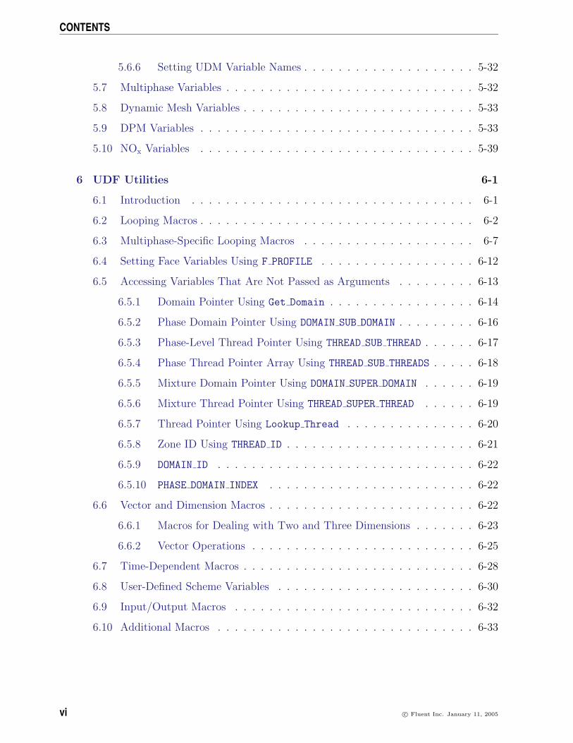
UDFs are called at predetermined times in the FLUENT solution process. However, theycan also be executed asynchronously (or ”on demand”) using an ON DEMAND function.If an EXECUTE AT END UDF is utilized, then FLUENT calls the function at the end of atimestep. Understanding the context in which UDFs are called within FLUENT’s solutionprocess may be important when you begin the process of writing UDF code, dependingon the type of UDF you are writing. The solver contains call-outs that are linked touser-defined functions that you write. Knowing the sequencing of function calls withinan iteration in the FLUENT solution process can help you determine which data arecurrent and available at any given time.
Segregated Solver
The solution process for the segregated solver (Figure 1.10.1) begins with a 3-step ini-tialization sequence that is executed outside the solution iteration loop. This sequencebegins by initializing equations to user-entered (or default) values taken from the FLU-ENT user interface. Next, user-defined PROFILE functions are called followed by a call toINIT UDFs. Initialization UDFs overwrite initialization values that were previously set.
The solution iteration loop begins with the execution of user-defined ADJUST functions.Following that, conservation equations are solved, progressing from the momentum equa-tions and subsequent pressure correction equation to the additional scalar equations thatare relevant to a particular calculation. Note that PROFILE and SOURCE UDFs are calledby each ”Solve” routine for the variable currently under consideration (e.g., species, ve-locity).
After the conservation equations, properties are updated including user-defined PROPERTY
UDFs. Thus, if your model involves the gas law, for example, the density will be updatedat this time using the updated temperature (and pressure and/or species mass fractions).A check for either convergence or additional requested iterations is done, and the loopeither continues or stops.
1-12 c© Fluent Inc. January 11, 2005
1.10 Calling Sequence of a UDF in the FLUENT Solution Process
Figure 1.10.1: Solution Procedure for the Segregated Solver
c© Fluent Inc. January 11, 2005 1-13

Overview
Coupled Solver
The solution process for the coupled solver (Figure 1.10.2) begins with a 3-step initializa-tion sequence that is executed outside the solution iteration loop. This sequence beginsby initializing equations to user-entered (or default) values taken from the FLUENT userinterface. Next, user-defined PROFILE functions are called followed by a call to INIT
UDFs. Initialization UDFs overwrite initialization values that were previously set.
The solution iteration loop begins with the execution of user-defined ADJUST functions.Next, FLUENT solves the governing equations of continuity, momentum, and (whereappropriate) energy simultaneously as a set, or vector, of equations. The remainder ofthe solution procedure is the same as the segregated solver (Figure 1.10.1).
Figure 1.10.2: Solution Procedure for the Coupled Solver
1-14 c© Fluent Inc. January 11, 2005
1.11 Special Considerations for Multiphase UDFs
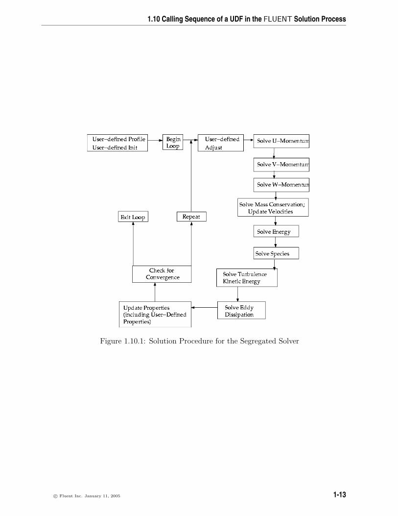
1.11 Special Considerations for Multiphase UDFs
In many cases, the UDF source code that you will write for a single-phase flow will bethe same as for a multiphase flow. For example, there will be no differences betweenthe C code for a single-phase boundary profile (defined using DEFINE PROFILE) and thecode for a multiphase profile, assuming that the function is accessing data only from thephase-level domain that it is hooked to in the graphical user interface. If your UDF isnot explicitly passed a pointer to the thread or domain structure that it requires, you willneed to use a special multiphase-specific utility (e.g., THREAD SUB THREAD) to retrieve it.This is discussed in Chapter 6: UDF Utilities.
See Appendix B for a complete list of general-purpose DEFINE macros and multiphase-specific DEFINE macros that can be used to define UDFs for multiphase model cases.
1.11.1 Multiphase-specific Data Types
In addition to the FLUENT-specific data types presented in Section 1.9: Data Typesin FLUENT, there are special thread and domain data structures that are specific tomultiphase UDFs. These data types are used to store properties and variables for themixture of all of the phases, as well as for each individual phase when a multiphase model(i.e., Mixture, VOF, Eulerian) is used.
In a multiphase application, the top-level domain is referred to as the ’superdomain’.Each phase occupies a domain referred to as a ’subdomain’. A third domain type,the ’interaction’ domain, is introduced to allow for the definition of phase interactionmechanisms. When mixture properties and variables are needed (a sum over phases),the superdomain is used for those quantities while the subdomain carries the informationfor individual phases. In single-phase, the concept of a mixture is used to represent thesum over all the species (components) while in multiphase it represents the sum over allthe phases. This distinction is important since FLUENT has the capability of handlingmultiphase multi-components, where, for example, a phase can consist of a mixture ofspecies.
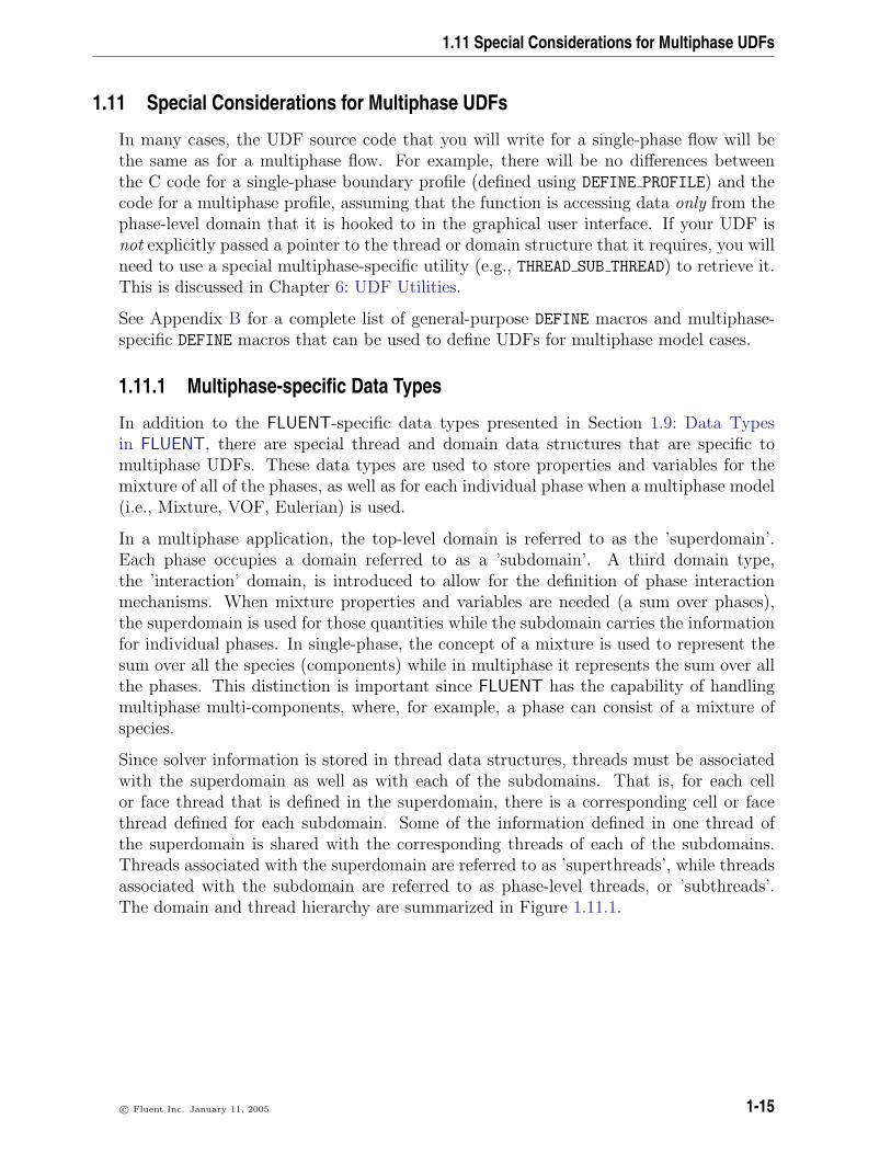
Since solver information is stored in thread data structures, threads must be associatedwith the superdomain as well as with each of the subdomains. That is, for each cellor face thread that is defined in the superdomain, there is a corresponding cell or facethread defined for each subdomain. Some of the information defined in one thread ofthe superdomain is shared with the corresponding threads of each of the subdomains.Threads associated with the superdomain are referred to as ’superthreads’, while threadsassociated with the subdomain are referred to as phase-level threads, or ’subthreads’.The domain and thread hierarchy are summarized in Figure 1.11.1.
c© Fluent Inc. January 11, 2005 1-15

Overview
Mixture domain, domain_id = 1
Primary phase domain, domain_id = 2
Secondary phase domain, domain_id = 4
Secondary phase domain, domain_id = 3
Mixture-level thread (e.g., inlet zone)
Mixture-level thread (e.g., fluid zone)
Interaction domainsdomain_id = 5, 6, 7
Phase-level threads for inlet zone identified by phase_domain_index
0
1
2
0
1
2
Figure 1.11.1: Domain and Thread Structure Hierarchy
Figure 1.11.1 introduces the concept of the domain id and phase domain index. Thedomain id can be used in UDFs to distinguish the superdomain from the primary andsecondary phase-level domains. The superdomain (mixture domain) domain id is alwaysassigned the value of 1. Interaction domains are also identified with the domain id. Thedomain ids are not necessarily ordered sequentially as shown in Figure 1.11.1.
The phase domain index can be used in UDFs to distinguish the primary phase-levelthreads from the secondary phase-level threads. For the primary phase-level thread, thephase domain index is always assigned the value of 0.
The data structures that are passed to a UDF depend on the multiphase model that isenabled, the property or term that is being modified, the DEFINE macro that is used,and the domain that is to be affected (mixture or phase). To better understand this,consider the differences between the Mixture and Eulerian multiphase models. In theMixture model, a single momentum equation is solved for a mixture whose properties aredetermined from the sum of its phases. In the Eulerian model, a momentum equationis solved for each phase. FLUENT allows you to directly specify a momentum source forthe mixture of phases (using DEFINE SOURCE) when the mixture model is used, but notfor the Eulerian model. For the latter case, you can specify momentum sources for theindividual phases. Hence, the multiphase model, as well as the term being modified bythe UDF, determines which domain or thread is required.
1-16 c© Fluent Inc. January 11, 2005

1.11 Special Considerations for Multiphase UDFs
UDFs that are hooked to the mixture of phases are passed superdomain (or mixture-level)structures, while functions that are hooked to a particular phase are passed subdomain(or phase-level) structures. DEFINE ADJUST and DEFINE INIT UDFs are hardwired to themixture-level domain. Other types of UDFs are hooked to different phase domains. Foryour convenience, Appendix B contains a list of multiphase models in FLUENT and thephase on which UDFs are specified for the given variables. From this information, youcan infer which domain structure is passed from the solver to the UDF.
c© Fluent Inc. January 11, 2005 1-17

Overview
1-18 c© Fluent Inc. January 11, 2005

Chapter 2. C Programming Basics for UDFs
This chapter contains an overview of C programming basics for UDFs.
• Section 2.1: Introduction
• Section 2.2: Commenting Your C Code
• Section 2.3: C Data Types in FLUENT
• Section 2.4: Constants
• Section 2.5: Variables
• Section 2.6: User-Defined Data Types
• Section 2.7: Casting
• Section 2.8: Functions
• Section 2.9: Arrays
• Section 2.10: Pointers
• Section 2.11: Control Statements
• Section 2.12: Common C Operators
• Section 2.13: C Library Functions
• Section 2.14: Macro Substitution Directive Using #define
• Section 2.14: File Inclusion Directive Using #include
• Section 2.15: Comparison with FORTRAN
2.1 Introduction
This chapter contains some basic information about the C programming language thatmay be helpful when writing UDFs in FLUENT. It is not intended to be used as a primeron C and assumes that you have some programming experience. There are many topicsand details that are not covered in this chapter including, for example, while and do-whilecontrol statements, unions, recursion, structures, and reading and writing files.
If you are unfamiliar with C or need information on C programming, consult any one ofthe available resource books on the subject (e.g., [2, 3]).
c© Fluent Inc. January 11, 2005 2-1

C Programming Basics for UDFs
2.2 Commenting Your C Code
It is good programming practice to document your C code with comments that are usefulfor explaining the purpose of the function. In a single line of code, your comments mustbegin with the /* identifier, followed by text, and end with the */ identifier as shown bythe following:
/* This is how I put a comment in my C program */
Comments that span multiple lines are bracketed by the same identifiers:
/* This is how I put a comment in my C program
that spans more
than one line. */
i Do not include a DEFINE macro name (e.g., DEFINE PROFILE) within acomment in your source code. This will cause a compilation error.
2.3 C Data Types in FLUENT
The UDF interpreter in FLUENT supports the following standard C data types:
int integer numberlong integer number of increased rangefloat floating point (real) numberdouble double-precision floating point (real) numberchar single byte of memory, enough to hold a character
Note that in FLUENT, real is a typedef that switches between float for single-precisionarithmetic, and double for double-precision arithmetic. Since the interpreter makes thisassignment automatically, it is good programming practice to use the real typedef whendeclaring all float and double data type variables in your UDF.
2-2 c© Fluent Inc. January 11, 2005
2.4 Constants
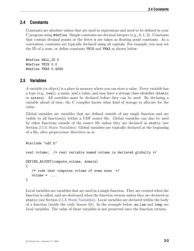
2.4 Constants
Constants are absolute values that are used in expressions and need to be defined in yourC program using #define. Simple constants are decimal integers (e.g., 0, 1, 2). Constantsthat contain decimal points or the letter e are taken as floating point constants. As aconvention, constants are typically declared using all capitals. For example, you may setthe ID of a zone, or define constants YMIN and YMAX as shown below:
#define WALL_ID 5
#define YMIN 0.0
#define YMAX 0.4064
2.5 Variables
A variable (or object) is a place in memory where you can store a value. Every variable hasa type (e.g., real), a name, and a value, and may have a storage class identifier (staticor extern). All variables must be declared before they can be used. By declaring avariable ahead of time, the C compiler knows what kind of storage to allocate for thevalue.
Global variables are variables that are defined outside of any single function and arevisible to all function(s) within a UDF source file. Global variables can also be usedby other functions outside of the source file unless they are declared as static (seeSection 2.5.3: Static Variables). Global variables are typically declared at the beginningof a file, after preprocessor directives as in
#include "udf.h"
real volume; /* real variable named volume is declared globally */
DEFINE_ADJUST(compute_volume, domain)
/* code that computes volume of some zone */
volume = ....
Local variables are variables that are used in a single function. They are created when thefunction is called, and are destroyed when the function returns unless they are declared asstatic (see Section 2.5.3: Static Variables). Local variables are declared within the bodyof a function (inside the curly braces ). In the example below, mu lam and temp arelocal variables. The value of these variables is not preserved once the function returns.
c© Fluent Inc. January 11, 2005 2-3

C Programming Basics for UDFs
DEFINE_PROPERTY(cell_viscosity, cell, thread)
real mu_lam; /* local variable */
real temp = C_T(cell, thread); /* local variable */
if (temp > 288.)
mu_lam = 5.5e-3;
else if (temp > 286.)
mu_lam = 143.2135 - 0.49725 * temp;
else
mu_lam = 1.;
return mu_lam;
2.5.1 Declaring Variables
A variable declaration begins with the data type (e.g., int), followed by the name of oneor more variables of the same type that are separated by commas. A variable declarationcan also contain an initial value, and always ends with a semicolon (;). Variable namesmust begin with a letter in C. A name can include letters, numbers, and the underscore( ) character. Note that the C preprocessor is case-sensitive (recognizes uppercase andlowercase letters as being different). Below are some examples of variable declarations.
int n; /* declaring variable n as an integer */
int i1, i2; /* declaring variables i1 and i2 as integers */
float tmax = 0.; /* tmax is a floating point real number
that is initialized to 0 */
real average_temp = 0.0; /* average_temp is a real number initialized
to 0.0 */
2-4 c© Fluent Inc. January 11, 2005

2.5 Variables
2.5.2 External Variables
If you have a global variable that is declared in one source code file, but a function inanother source file needs to use it, then it must be defined in the other source file asan external variable. To do this, simply precede the variable declaration by the wordextern as in
extern real volume;
If there are several files referring to that variable then it is convenient to include theextern definition in a header (.h) file, and include the header file in all of the .c filesthat want to use the external variable. Only one .c file should have the declaration ofthe variable without the extern keyword. Below is an example that demonstrates theuse of a header file.
i extern can be used only in compiled UDFs.
c© Fluent Inc. January 11, 2005 2-5

C Programming Basics for UDFs
Example
Suppose that there is a global variable named volume that is declared in a C source filenamed file1.c
#include "udf.h"
real volume; /* real variable named volume is declared globally */
DEFINE_ADJUST(compute_volume, domain)
/* code that computes volume of some zone */
volume = ....
If multiple source files want to use volume in their computations, then volume can bedeclared as an external variable in a header file (e.g., extfile.h)
/* extfile.h
Header file that contains the external variable declaration for
volume */
extern real volume;
Now another file named file2.c can declare volume as an external variable by simplyincluding extfile.h.
/* file2.c
#include "udf.h"
#include "extfile.h" /* header file containing extern declaration
is included */
DEFINE_SOURCE(heat_source,c,t,ds,eqn)
/* code that computes the per unit volume source using the total
volume computed in the compute_volume function from file1.c */
real total_source = ...;
real source;
source = total_source/volume;
return source;
2-6 c© Fluent Inc. January 11, 2005

2.5 Variables
2.5.3 Static Variables
The static operator has different effects depending on whether it is applied to local orglobal variables. When a local variable is declared as static the variable is preventedfrom being destroyed when a function returns from a call. In other words, the value of thevariable is preserved. When a global variable is declared as static the variable is “fileglobal”. It can be used by any function within the source file in which it is declared, butis prevented from being used outside the file, even if is declared as external. Functionscan also be declared as static. A static function is visible only to the source file inwhich it is defined.
i static variables and functions can be declared only in compiled UDFsource files.
Example - Static Global Variable
/* mysource.c /*
#include "udf.h"
static real abs_coeff = 1.0; /* static global variable */
/* used by both functions in this source file but is
not visible to the outside */
DEFINE_SOURCE(energy_source, c, t, dS, eqn)
real source; /* local variable
int P1 = ....; /* local variable
value is not preserved when function returns */
dS[eqn] = -16.* abs_coeff * SIGMA_SBC * pow(C_T(c,t),3.);
source =-abs_coeff *(4.* SIGMA_SBC * pow(C_T(c,t),4.) - C_UDSI(c,t,P1));
return source;
DEFINE_SOURCE(p1_source, c, t, dS, eqn)
real source;
int P1 = ...;
dS[eqn] = -abs_coeff;
source = abs_coeff *(4.* SIGMA_SBC * pow(C_T(c,t),4.) - C_UDSI(c,t,P1));
return source;
c© Fluent Inc. January 11, 2005 2-7

C Programming Basics for UDFs
2.6 User-Defined Data Types
C also allows you to create user-defined data types using structures and typedef. (Forinformation about structures in C, see [2].) An example of a structured list definition isshown below.
i typedef can only be used for compiled UDFs.
Example
typedef struct listint a;
real b;
int c; mylist; /* mylist is type structure list
mylist x,y,z; x,y,z are type structure list */
2.7 Casting
You can convert from one data type to another by casting. A cast is denoted by type,where the type is int, float, etc., as shown in the following example:
int x = 1;
real y = 3.14159;
int z = x+((int) y); /* z = 4 */
2.8 Functions
Functions perform tasks. Tasks may be useful to other functions defined within the samesource code file, or they may be used by a function external to the source file. A functionhas a name (that you supply) and a list of zero or more arguments that are passed to it.Note that your function name cannot contain a number in the first couple of characters.A function has a body enclosed within curly braces that contains instructions for carryingout the task. A function may return a value of a particular type. C functions pass databy value.
Functions either return a value of a particular data type (e.g., real), or do not return anyvalue if they are of type void. To determine the return data type for the DEFINE macroyou will use to define your UDF, look at the macro’s corresponding #define statementin the udf.h file or see Appendix A for a listing.
i C functions cannot alter their arguments. They can, however, alter thevariables that their arguments point to.
2-8 c© Fluent Inc. January 11, 2005

2.9 Arrays
2.9 Arrays
Arrays of variables can be defined using the notation name[size], where name is thevariable name and size is an integer that defines the number of elements in the array.The index of a C array always begins at 0.
Arrays of variables can be of different data types as shown below.
Examples
int a[10], b[10][10];
real radii[5];
a[0] = 1; /* a 1-Dimensional array of variable a */
radii[4] = 3.14159265; /* a 1-Dimensional array of variable radii */
b[10][10] = 4; /* a 2-Dimensional array of variable b */
2.10 Pointers
A pointer is a variable that contains an address in memory where the value referencedby the pointer is stored. In other words, a pointer is a variable that points to anothervariable by referring to the other variable’s address. Pointers contain memory addresses,not values. Pointer variables must be declared in C using the * notation. Pointers arewidely used to reference data stored in structures and to pass data among functions (bypassing the addresses of the data).
For example,
int *ip;
declares a pointer named ip that points to an integer variable. Now suppose you wantto assign an address to pointer ip. To do this, you can use the & notation. For example,
ip = &a;
assigns the address of variable a to pointer ip.
You can retrieve the value of variable a that pointer ip is pointing to by
*ip
c© Fluent Inc. January 11, 2005 2-9
C Programming Basics for UDFs
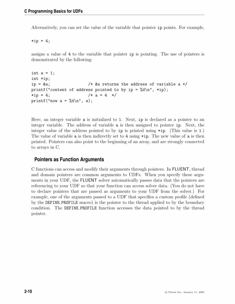
Alternatively, you can set the value of the variable that pointer ip points. For example,
*ip = 4;
assigns a value of 4 to the variable that pointer ip is pointing. The use of pointers isdemonstrated by the following:
int a = 1;
int *ip;
ip = &a; /* &a returns the address of variable a */
printf("content of address pointed to by ip = %d\n", *ip);
*ip = 4; /* a = 4 */
printf("now a = %d\n", a);
Here, an integer variable a is initialized to 1. Next, ip is declared as a pointer to aninteger variable. The address of variable a is then assigned to pointer ip. Next, theinteger value of the address pointed to by ip is printed using *ip. (This value is 1.)The value of variable a is then indirectly set to 4 using *ip. The new value of a is thenprinted. Pointers can also point to the beginning of an array, and are strongly connectedto arrays in C.
Pointers as Function Arguments
C functions can access and modify their arguments through pointers. In FLUENT, threadand domain pointers are common arguments to UDFs. When you specify these argu-ments in your UDF, the FLUENT solver automatically passes data that the pointers arereferencing to your UDF so that your function can access solver data. (You do not haveto declare pointers that are passed as arguments to your UDF from the solver.) Forexample, one of the arguments passed to a UDF that specifies a custom profile (definedby the DEFINE PROFILE macro) is the pointer to the thread applied to by the boundarycondition. The DEFINE PROFILE function accesses the data pointed to by the threadpointer.
2-10 c© Fluent Inc. January 11, 2005

2.11 Control Statements
2.11 Control Statements
You can control the order in which statements are executed in your C program usingcontrol statements like if, if-else, and for loops. Control statements make decisionsabout what is to be executed next in the program sequence.
2.11.1 if Statement
An if statement is a type of conditional control statement. The format of an if statementis:
if (logical-expression)
statements
where logical-expression is the condition to be tested, and statements are the linesof code that are to be executed if the condition is met.
Example
if (q != 1)
a = 0; b = 1;
2.11.2 if-else Statement
if-else statements are another type of conditional control statement. The format of anif-else statement is:
if (logical-expression)
statements
else
statements
where logical-expression is the condition to be tested, and the first set of statementsare the lines of code that are to be executed if the condition is met. If the condition isnot met, then the statements following else are executed.
c© Fluent Inc. January 11, 2005 2-11

C Programming Basics for UDFs
Example
if (x < 0.)
y = x/50.;
else
x = -x;
y = x/25.;
The equivalent FORTRAN code is shown below for comparison.
IF (X.LT.0.) THEN
Y = X/50.
ELSE
X = -X
Y = X/25.
ENDIF
2.11.3 for Loops
for loops are control statements that are a basic looping construct in C. They are anal-ogous to do loops in FORTRAN. The format of a for loop is
for (begin ; end ; increment)
statements
where begin is the expression that is executed at the beginning of the loop; end is thelogical expression that tests for loop termination; and increment is the expression thatis executed at the end of the loop iteration (usually incrementing a counter).
Example
/* Print integers 1-10 and their squares */
int i, j, n = 10;
for (i = 1 ; i <= n ; i++)
j = i*i;
printf("%d %d\n",i,j);
2-12 c© Fluent Inc. January 11, 2005
2.12 Common C Operators
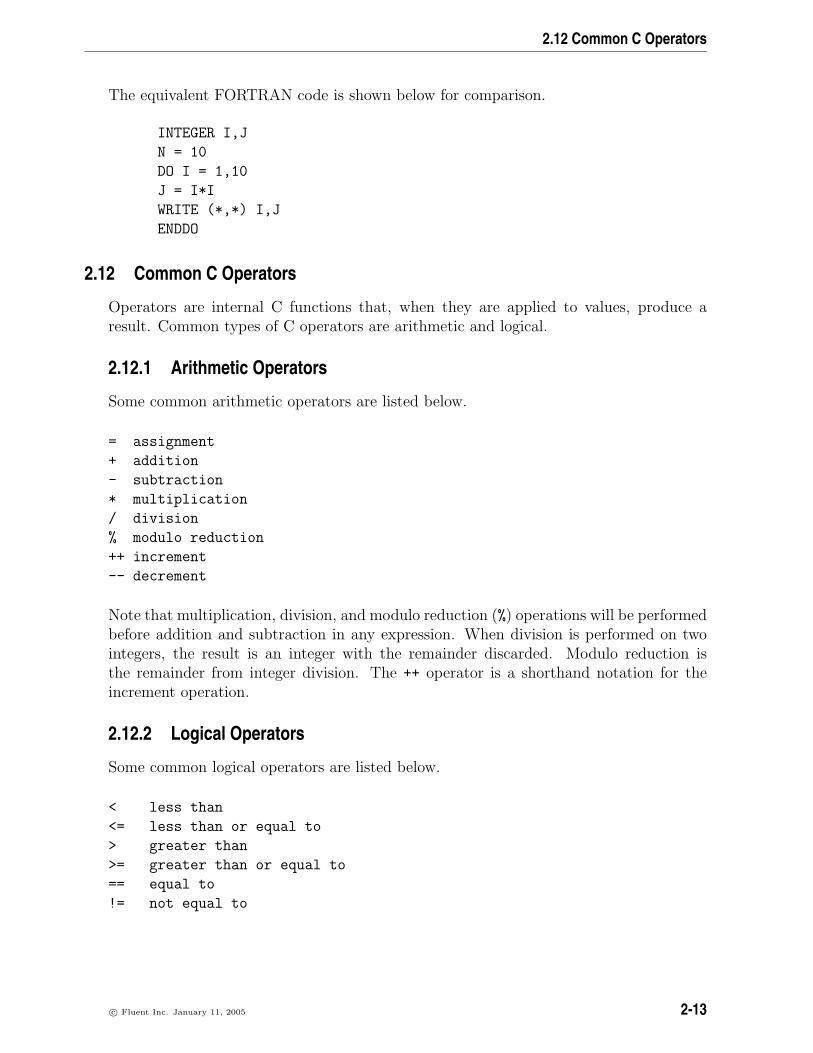
The equivalent FORTRAN code is shown below for comparison.
INTEGER I,J
N = 10
DO I = 1,10
J = I*I
WRITE (*,*) I,J
ENDDO
2.12 Common C Operators
Operators are internal C functions that, when they are applied to values, produce aresult. Common types of C operators are arithmetic and logical.
2.12.1 Arithmetic Operators
Some common arithmetic operators are listed below.
= assignment
+ addition
- subtraction
* multiplication
/ division
% modulo reduction
++ increment
-- decrement
Note that multiplication, division, and modulo reduction (%) operations will be performedbefore addition and subtraction in any expression. When division is performed on twointegers, the result is an integer with the remainder discarded. Modulo reduction isthe remainder from integer division. The ++ operator is a shorthand notation for theincrement operation.
2.12.2 Logical Operators
Some common logical operators are listed below.
< less than
<= less than or equal to
> greater than
>= greater than or equal to
== equal to
!= not equal to
c© Fluent Inc. January 11, 2005 2-13

C Programming Basics for UDFs
2.13 C Library Functions
C compilers include a library of standard mathematical and I/O functions that you canuse when you write your UDF code. Lists of standard C library functions are presentedin the following sections. Definitions for standard C library functions can be found invarious header files (e.g., global.h). These header files are all included in the udf.h file.
2.13.1 Trigonometric Functions
The trigonometric functions shown below are computed (with one exception) for thevariable x. Both the function and the argument are double-precision real variables. Thefunction acos(x) is the arccosine of the argument x, cos−1(x). The function atan2(x,y)
is the arctangent of x/y, tan−1(x/y). The function cosh(x) is the hyperbolic cosinefunction, etc.
double acos (double x); returns the arcosine of xdouble asin (double x); returns the arcsine of xdouble atan (double x); returns the arctangent of xdouble atan2 (double x, double y); returns the arctangent of x/ydouble cos (double x); returns the cosine of xdouble sin (double x); returns the sine of xdouble tan (double x); returns the tangent of xdouble cosh (double x); returns the hyperbolic cosine of xdouble sinh (double x); returns the hyperbolic sine of xdouble tanh (double x); returns the hyperbolic tangent of x
2.13.2 Miscellaneous Mathematical Functions
The C functions shown on the left below correspond to the mathematical functions shownon the right.
double sqrt (double x);√x
double pow(double x, double y); xy
double exp (double x); ex
double log (double x); ln(x)double log10 (double x); log10(x)double fabs (double x); | x |double ceil (double x); smallest integer not less than xdouble floor (double x); largest integer not greater than x
2-14 c© Fluent Inc. January 11, 2005

2.13 C Library Functions
2.13.3 Standard I/O Functions
A number of standard input and output (I/O) functions are available in C and in FLU-ENT. They are listed below. All of the functions work on a specified file except forprintf, which displays information that is specified in the argument of the function.The format string argument is the same for printf, fprintf, and fscanf. Note thatall of these standard C I/O functions are supported by the interpreter, so you can usethem in either interpreted or compiled UDFs. For more information about standard I/Ofunctions in C, you should consult a reference guide (e.g., [2]).
Common C I/O Functions
fopen("filename", "mode"); opens a filefclose(fp); closes a fileprintf("format", ...); formatted print to the consolefprintf(fp, "format", ...); formatted print to a filefscanf(fp, "format", ...); formatted read from a file
i It is not possible to use the scanf C function in FLUENT.
fopen
FILE *fopen(char *filename, char *mode);
The function fopen opens a file in the mode that you specify. It takes two arguments:filename and mode. filename is a pointer to the file you want to open. mode is themode in which you want the file opened. The options for mode are read "r", write "w",and append "a”. Both arguments must be enclosed in quotes. The function returns apointer to the file that is to be opened.
Before using fopen, you will first need to define a local pointer of type FILE that isdefined in stdio.h (e.g., fp). Then, you can open the file using fopen, and assign it tothe local pointer as shown below. Recall that stdio.c is included in the udf.h file, soyou don’t have to include it in your function.
FILE *fp; /* define a local pointer fp of type FILE */
fp = fopen("data.txt","r"); /* open a file named data.txt in
read-only mode and assign it to fp */
c© Fluent Inc. January 11, 2005 2-15

C Programming Basics for UDFs
fclose
int fclose(FILE *fp);
The function fclose closes a file that is pointed to by the local pointer passed as anargument (e.g., fp).
fclose(fp); /* close the file pointed to by fp */
printf
int printf(char *format, ...);
The function printf is a general-purpose printing function that prints to the consolein a format that you specify. The first argument is the format string. It specifies howthe remaining arguments are to be displayed in the console window. The format stringis defined within quotes. The value of the replacement variables that follow the formatstring will be substituted in the display for all instances of %type. The % character is usedto designate the character type. Some common format characters are: %d for integers,%f for floating point numbers, and %e for floating point numbers in exponential format(with e before the exponent). The format string for printf is the same as for fprintf
and fscanf.
In the example below, the text Content of variable a is: will be displayed in theconsole window, and the value of the replacement variable, a, will be substituted in themessage for all instances of %d.
Example:
int a = 5;
printf("Content of variable a is: %d\n", a); /* \n denotes a new line */
i (UNIX only) It is recommended that you use the Fluent Inc. Message
utility instead of printf for compiled UDFs. See Section 6.9: Message fordetails on the Message macro.
fprintf
int fprintf(FILE *fp, char *format, ...);
The function fprintf writes to a file that is pointed to by fp, in a format that you specify.The first argument is the format string. It specifies how the remaining arguments areto be written to the file. The format string for fprintf is the same as for printf andfscanf.
2-16 c© Fluent Inc. January 11, 2005

2.13 C Library Functions
Example:
FILE *fp;
fprintf(fp,"%12.4e %12.4e %5d\n",x_array[j][0], x_array[j][1], noface);
int data1 = 64.25;
int data2 = 97.33;
fprintf(fp, "%4.2d %4.2d\n", data1, data2);
fscanf
int fscanf(FILE *fp, char *format, ...);
The function fscanf reads from a file that is pointed to by fp, in a format that youspecify. The first argument is the format string. It specifies how the data that is tobe read is to be interpreted. The replacement variables that follow the format stringare used to store values that are read. The replacement variables are preceded by the& character. Note that the format string for fscanf is the same as for fprintf andprintf.
In the example below, two floating point numbers are read from the file pointed to byfp, and are stored in the variables f1 and f2.
Example:
FILE *fp;
fscanf(fp, "%f %f", &f1, &f2);
i You cannot use the scanf I/O function in FLUENT. You must use fscanf
instead.
c© Fluent Inc. January 11, 2005 2-17

C Programming Basics for UDFs
2.14 Preprocessor Directives
The UDF interpreter supports C preprocessor directives including #define and #include.
Macro Substitution Directive Using #define
When you use the #define macro substitution directive, the C preprocessor (e.g., cpp)performs a simple substitution and expands the occurrence of each argument in macrousing the replacement-text.
#define macro replacement-text
For example, the macro substitution directive given by
#define RAD 1.2345
will cause the preprocessor to replace all instances of the variable RAD in your UDF withthe number 1.2345. There may be many references to the variable RAD in your function,but you only have to define it once in the macro directive; the preprocessor does the workof performing the substitution throughout your code.
In another example
#define AREA_RECTANGLE(X,Y) ((X)*(Y))
all of the references to AREA RECTANGLE(X,Y) in you UDF are replaced by the productof (X) and (Y).
File Inclusion Directive Using #include
When you use the #include file inclusion directive, the C preprocessor replaces the line#include filename with the contents of the named file.
#include "filename"
The file you name must reside in your current directory. The only exception to this ruleis the udf.h file, which is read automatically by the FLUENT solver.
For example, the file inclusion directive given by
#include "udf.h"
will cause the udf.h file to be included with your source code. The FLUENT solverautomatically reads the udf.h file from the Fluent.Inc/fluent6.x/src/ directory.
2-18 c© Fluent Inc. January 11, 2005

2.15 Comparison with FORTRAN
2.15 Comparison with FORTRAN
Many simple C functions are similar to FORTRAN function subroutines as shown in theexample below:
A simple C function An equivalent FORTRAN function
int myfunction(int x) INTEGER FUNCTION MYFUNCTION(X)
int x,y,z; INTEGER X,Y,Z
y = 11; Y = 11
z = x+y; Z = X+Y
printf("z = %d",z); WRITE (*,100) Z
return z; MYFUNCTION = Z
END
c© Fluent Inc. January 11, 2005 2-19

C Programming Basics for UDFs
2-20 c© Fluent Inc. January 11, 2005

Chapter 3. A Step-by-Step UDF Example
This chapter contains an example that utilizes a 7-step process to code a UDF and useit effectively in your FLUENT model.
3.1 Process Overview1. Define your problem. (Section 3.1.1: Step 1: Define Your Problem)
2. Create a C source code file. (Section 3.1.2: Step 2: Create a C Source File)
3. Start FLUENT and read in (or set up) the case file. (Section 3.1.3: Step 3: StartFLUENT and Read (or Set Up) the Case File)
4. Interpret or compile the source file. (Section 3.1.4: Step 4: Interpret or Compilethe Source File)
5. Hook the UDF to FLUENT. (Section 3.1.5: Step 5: Hook Your UDF to FLUENT)
6. Run the calculation. (Section 3.1.6: Step 6: Run the Calculation)
7. Analyze the numerical solution and compare it to expected results. (Section 3.1.7: Step7: Analyze the Numerical Solution and Compare to Expected Results)
To begin the process, you’ll need to define the problem you wish to solve using a UDF(Step 1). For example, suppose you want to use a UDF to define a custom boundaryprofile for your model. You will first need to define the set of mathematical equationsthat describes the profile.
Next you will need to translate the mathematical equation (conceptual design) into afunction written in the C programming language (Step 2). You can do this using anytext editor. Save the file with a .c suffix (e.g., udfexample.c) in your working directory.
Once you have written the C function, you are ready to start FLUENT and read in (or setup) your case file (Step 3). You will then need to interpret or compile the source code,debug it (Step 4), and then hook the function to FLUENT (Step 5). Finally you’ll runthe calculation (Step 6), analyze the results from your simulation, and compare themto expected results (Step 7). You may loop through this entire process more than once,depending on the results of your analysis. Follow the step-by-step process in the sectionsbelow to see how this is done.
c© Fluent Inc. January 11, 2005 3-1

A Step-by-Step UDF Example
3.1.1 Step 1: Define Your Problem
The first step in creating a UDF and using it in your FLUENT model involves definingyour model equation(s).
Consider the turbine vane illustrated in Figure 3.1.1. An unstructured grid is used tomodel the flow field surrounding the vane. The domain extends from a periodic boundaryon the bottom to an identical one on the top, a velocity inlet on the left, and a pressureoutlet on the right.
GridTurbine Vane (1551 cells, 2405 faces, 893 nodes)
Figure 3.1.1: The Grid for the Turbine Vane Example
A flow field in which a constant x velocity is applied at the inlet will be compared withone where a parabolic x velocity profile is applied. The results of a constant-velocityapplied field (of 20 m/s) at the inlet are shown in Figures 3.1.2 and 3.1.3. The initialconstant-velocity field is distorted as the flow moves around the turbine vane.
Now suppose that you want to impose a non-uniform x velocity to the turbine vane inlet,which is described by the profile
vx = 20− 20(
y
0.0745
)2
(3.1-1)
where the variable y is 0.0 at the center of the inlet, and extends to values of ± 0.0745 mat the top and bottom. Thus the x velocity will be 20 m/s at the center of the inlet, and0 at the edges.
3-2 c© Fluent Inc. January 11, 2005

3.1 Process Overview
Contours of Velocity Magnitude (m/s)Turbine Vane (1551 cells, 2405 faces, 893 nodes)
5.98e+01
5.42e+01
4.86e+01
4.30e+01
3.74e+01
3.19e+01
2.63e+01
2.07e+01
1.51e+01
9.54e+00
3.96e+00
Figure 3.1.2: Velocity Magnitude Contours for a Constant Inlet x Velocity
Velocity Vectors Colored By Velocity Magnitude (m/s)Turbine Vane (1551 cells, 2405 faces, 893 nodes)
6.11e+01
5.52e+01
4.93e+01
4.34e+01
3.75e+01
3.16e+01
2.57e+01
1.98e+01
1.39e+01
7.96e+00
2.05e+00
Figure 3.1.3: Velocity Vectors for a Constant Inlet x Velocity
c© Fluent Inc. January 11, 2005 3-3
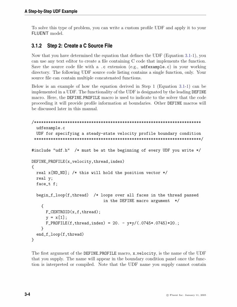
A Step-by-Step UDF Example
To solve this type of problem, you can write a custom profile UDF and apply it to yourFLUENT model.
3.1.2 Step 2: Create a C Source File
Now that you have determined the equation that defines the UDF (Equation 3.1-1), youcan use any text editor to create a file containing C code that implements the function.Save the source code file with a .c extension (e.g., udfexample.c) in your workingdirectory. The following UDF source code listing contains a single function, only. Yoursource file can contain multiple concatenated functions.
Below is an example of how the equation derived in Step 1 (Equation 3.1-1) can beimplemented in a UDF. The functionality of the UDF is designated by the leading DEFINE
macro. Here, the DEFINE PROFILE macro is used to indicate to the solver that the codeproceeding it will provide profile information at boundaries. Other DEFINE macros willbe discussed later in this manual.
/**********************************************************************
udfexample.c
UDF for specifying a steady-state velocity profile boundary condition
**********************************************************************/
#include "udf.h" /* must be at the beginning of every UDF you write */
DEFINE_PROFILE(x_velocity,thread,index)
real x[ND_ND]; /* this will hold the position vector */
real y;
face_t f;
begin_f_loop(f,thread) /* loops over all faces in the thread passed
in the DEFINE macro argument */
F_CENTROID(x,f,thread);
y = x[1];
F_PROFILE(f,thread,index) = 20. - y*y/(.0745*.0745)*20.;
end_f_loop(f,thread)
The first argument of the DEFINE PROFILE macro, x velocity, is the name of the UDFthat you supply. The name will appear in the boundary condition panel once the func-tion is interpreted or compiled. Note that the UDF name you supply cannot contain
3-4 c© Fluent Inc. January 11, 2005

3.1 Process Overview
a number as the first character. The equation that is defined by the function will beapplied to all cell faces (identified by f in the face loop) on a given boundary zone(identified by thread). The thread is defined automatically when you hook the UDFto a particular boundary in the FLUENT graphical user-interface. The index is definedautomatically through the begin f loop utility. In this UDF, the begin f loop macro(Section 6.2: Looping Macros) is used to loop through all cell faces in the boundaryzone. For each face, the coordinates of the face centroid are accessed by F CENTROID
(Section 5.2.4: Connectivity Variables). The y coordinate y is used in the parabolicprofile equation and the returned velocity is assigned to the face through F PROFILE.begin f loop and F PROFILE (Section 6.4: Setting Face Variables Using F PROFILE) areFluent-supplied macros.
3.1.3 Step 3: Start FLUENT and Read (or Set Up) the Case File
Once you have created the source code for your UDF, you are ready to begin the problemsetup in FLUENT.
1. Start FLUENT from your working directory.
2. Read (or set up) your case file.
3.1.4 Step 4: Interpret or Compile the Source File
You are now ready to interpret or compile the profile UDF named x velocity) that youcreated in Step 2 and is contained within the source file named udfexample.c. In general,you must compile your function as a compiled UDF if the source code contains structuredreference calls or other elements of C that are not handled by the FLUENT interpreter.To determine whether you should compile or interpret your UDF, see Section 1.6.1: Dif-ferences Between Interpreted and Compiled UDFs.
c© Fluent Inc. January 11, 2005 3-5

A Step-by-Step UDF Example
Interpret the Source File
Follow the procedure below to interpret your source file in FLUENT. For more informationon interpreting UDFs, see Chapter 7: Interpreting UDF Source Files.
i Note that this step does not apply to Windows parallel networks. SeeSection 7.2: Interpreting a UDF Source File Using the Interpreted UDFsPanel for details.
1. Open the Interpreted UDFs panel.
Define −→ User-Defined −→ Functions −→ Interpreted...
Figure 3.1.4: The Interpreted UDFs Panel
3-6 c© Fluent Inc. January 11, 2005

3.1 Process Overview
2. In the Interpreted UDFs panel, select the UDF source file by either typing thecomplete path in the Source File Name field or click Browse... to use the browser.This will open the Select File panel (Figure 3.1.5).
Figure 3.1.5: The Select File Panel
3. In the Select File panel, highlight the directory path underDirectories (e.g., /nfs/homeserver/home/clb/mywork/), and the desired file(e.g., udfexample.c) under Files, and click OK. This will close the Select File paneland display the path to the selected source file in the Interpreted UDFs panel.
4. In the Interpreted UDFs panel, specify the C preprocessor to be used in the CPPCommand Name field. You can keep the default cpp or you can select Use Con-tributed CPP to use the preprocessor supplied by Fluent Inc.
If you installed the /contrib component from the “PrePost” CD, then by default,the cpp preprocessor will appear in the panel. For Windows NT users, the standardWindows NT installation of the FLUENT product includes the cpp preprocessor.
For Windows NT systems, if you are using the Microsoft compiler, then use thecommand cl -E.
c© Fluent Inc. January 11, 2005 3-7

A Step-by-Step UDF Example
i Note that the default CPP Command Name is different for 2d and 3d cases.The default preprocessor is cpp and cc -E for a 2d and 3d case, respec-tively.
5. Keep the default Stack Size setting of 10000, unless the number of local variablesin your function will cause the stack to overflow. In this case, set the Stack Size toa number that is greater than the number of local variables used.
6. Keep the Display Assembly Listing option on if you want a listing of assembly lan-guage code to appear in your console window when the function interprets. Thisoption will be saved in your case file, so that when you read the case in a subsequentFLUENT session, the assembly code will be automatically displayed.
7. Click Interpret to interpret your UDF. If the Display Assembly Listing option waschosen, then the assembly code will appear in the console window when the UDFis interpreted, as shown below.
x_velocity:.local.pointer thread (r0).local.int nv (r1)
0 .local.end0 save
.local.int f (r3)1 push.int 0
.local.pointer x (r4)3 begin.data 8 bytes, 0 bytes initialized:7 save. .. .. .
156 pre.inc.int f (r3)158 pop.int159 b .L3 (22)
.L2:161 restore162 restore163 ret.v
i Note that if your compilation is unsuccessful, then FLUENT will report anerror and you will need to debug your program. See Section 7.3: CommonErrors Made While Interpreting A Source File for details.
8. Click Close when the interpreter has finished.
3-8 c© Fluent Inc. January 11, 2005

3.1 Process Overview
9. Write the case file. The interpreted UDF, named x velocity, will be saved withthe case file so that the function will be automatically interpreted whenever thecase is subsequently read.
Compile the Source File
You can compile your UDF using the text user interface (TUI) or the graphical userinterface (GUI) in FLUENT. The GUI option for compiling a source file on a UNIX systemis discussed below. For details about compiling on other platforms (e.g., Windows) usingthe TUI to compile your function, or for general questions about compiling UDFs inFLUENT see Chapter 8: Compiling UDF Source Files.
1. Make sure that the UDF source file (e.g., udfexample.c) is in the same directorythat contains your case and data file.
2. Start FLUENT from your working directory.
3. Read (or set up) your case file.
4. Open the Compiled UDFs panel (Figure 3.1.6).
Define −→ User-Defined −→ Functions −→ Compiled...
Figure 3.1.6: The Compiled UDFs Panel
5. Click Add... under Source Files in the Compiled UDFs panel. This will open theSelect File panel (Figure 3.1.7).
c© Fluent Inc. January 11, 2005 3-9
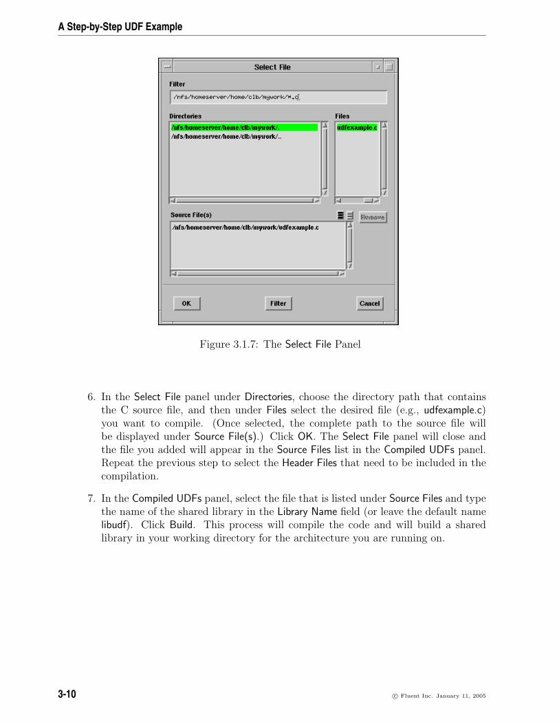
A Step-by-Step UDF Example
Figure 3.1.7: The Select File Panel
6. In the Select File panel under Directories, choose the directory path that containsthe C source file, and then under Files select the desired file (e.g., udfexample.c)you want to compile. (Once selected, the complete path to the source file willbe displayed under Source File(s).) Click OK. The Select File panel will close andthe file you added will appear in the Source Files list in the Compiled UDFs panel.Repeat the previous step to select the Header Files that need to be included in thecompilation.
7. In the Compiled UDFs panel, select the file that is listed under Source Files and typethe name of the shared library in the Library Name field (or leave the default namelibudf). Click Build. This process will compile the code and will build a sharedlibrary in your working directory for the architecture you are running on.
3-10 c© Fluent Inc. January 11, 2005

3.1 Process Overview
As the compile/build process begins, a Warning dialog box will appear, remindingyou that the UDF source file must be in the directory that contains your case anddata files (i.e., your working directory). If you have an existing library directory(e.g., libudf) then you will need to remove it prior to the build, to ensure that thelatest files are used. Click OK to close the dialog box and resume the compile/buildprocess. The results of the build will be displayed on the console window. You canview the compilation history in the ‘log’ file that is saved in your working directory.
i If the compile/build is unsuccessful, then FLUENT will report an errorand you will need to debug your program before continuing. See Sec-tion 8.6: Common Errors When Building and Loading a Shared Libraryfor a list of common errors.
8. Click Load to load the shared library into FLUENT. The console will report thatthe library has been opened and the function (e.g., x velocity) loaded.
Opening library "libudf"...
Library "libudf/lnx86/2d/libudf.so" opened
x_velocity
Done.
See Chapter 8: Compiling UDF Source Files for more information on the com-pile/build process.
c© Fluent Inc. January 11, 2005 3-11

A Step-by-Step UDF Example
3.1.5 Step 5: Hook Your UDF to FLUENT
Now that you have interpreted or compiled your UDF following the methods outlined inStep 4, you are ready to hook the function to FLUENT using a graphical user interfacepanel. The name you supplied in the DEFINE macro argument (e.g., x velocity) willappear in graphics panels in FLUENT. You will hook the profile UDF in this sampleproblem to the Velocity Inlet boundary condition panel.
1. Open the Velocity Inlet panel.
Define −→ Boundary Conditions...
Figure 3.1.8: The Velocity Inlet Panel
2. In the drop-down list for X-Velocity, choose udf x velocity, the name that was givento the function in our sample problem. Once selected, the UDF will be used in thecalculation, and the default value will be grayed-out in the X-Velocity field. ClickOK to accept the new boundary condition and close the panel.
3.1.6 Step 6: Run the Calculation
Run the calculation as usual.
Solve −→Iterate...
3-12 c© Fluent Inc. January 11, 2005

3.1 Process Overview
3.1.7 Step 7: Analyze the Numerical Solution and Compare to ExpectedResults
Once the solution is run to convergence, obtain a revised velocity field. The velocitymagnitude contours for the parabolic inlet x velocity are shown in Figure 3.1.9, andcan be compared to the results of a constant-velocity field of 20 m/sec (Figure 3.1.2).For the constant velocity condition, the flow field is distorted as the flow moves aroundthe turbine vane. The velocity field for the imposed parabolic profile, however, shows amaximum at the center of the inlet, which drops to zero at the edges.
Contours of Velocity Magnitude (m/s)Turbine Vane (1551 cells, 2405 faces, 893 nodes)
4.46e+01
4.05e+01
3.64e+01
3.23e+01
2.83e+01
2.42e+01
2.01e+01
1.60e+01
1.19e+01
7.78e+00
3.68e+00
Figure 3.1.9: Velocity Magnitude Contours for a Parabolic Inlet x Velocity
c© Fluent Inc. January 11, 2005 3-13

A Step-by-Step UDF Example
3-14 c© Fluent Inc. January 11, 2005
Chapter 4. Defining a UDF Using a DEFINE Macro
This chapter contains descriptions of predefined macros provided by Fluent Inc. that youwill need to use to define your UDF. These macros are referred to as DEFINE macros.
The chapter is organized in the following sections:
• Section 4.1: Introduction
• Section 4.2: Model-Independent DEFINE Macros
• Section 4.3: Model-Dependent DEFINE Macros
• Section 4.4: Multiphase DEFINE Macros
• Section 4.5: Dynamic Mesh DEFINE Macros
• Section 4.6: DPM DEFINE Macros
4.1 Introduction
DEFINE macros have been grouped into the following five categories:
• model-independent
• model-dependent
• multiphase
• dynamic mesh model
• discrete phase model (DPM)
For each of the DEFINE macros listed in this chapter, a source code example of a UDFthat uses it is provided, where available. Many of the examples make extensive use ofother macros discussed in later chapters on solver access (Chapter 5: Macros for AccessingFLUENT Solver Variables) and utilities (Chapter 6: UDF Utilities). Note that not all ofthe examples in the chapter are complete functions that can be executed as stand-alonefunctions in FLUENT. Examples are intended to demonstrate DEFINE macro usage only.
Special care must be taken for some serial UDFs that will be run in parallel FLUENT.See Chapter 10: Parallel UDF Usage for details.
c© Fluent Inc. January 11, 2005 4-1

Defining a UDF Using a DEFINE Macro
Definitions for all DEFINE macros are contained in the udf.h header file. For your con-venience, they are listed in Appendix A.
i Note that all of the arguments to a DEFINE macro need to be placed on thesame line in your source code. Splitting the DEFINE statement onto severallines will result in a compilation error.
4.2 Model-Independent DEFINE Macros
The DEFINE macros presented in this section implement general solver functions thatare independent of the model(s) you are using in FLUENT. Table 4.2.1 provides a quickreference guide to the DEFINE macros, the functions they are used to define, and the panelswhere they are activated in FLUENT. Definitions of each DEFINE macro are contained inthe udf.h header file and are provided in Appendix A.
• DEFINE ADJUST (Section 4.2.1: DEFINE ADJUST)
• DEFINE EXECUTE AT END (Section 4.2.2: DEFINE EXECUTE AT END)
• DEFINE EXECUTE FROM GUI (Section 4.2.3: DEFINE EXECUTE FROM GUI)
• DEFINE EXECUTE ON LOADING (Section 4.2.4: DEFINE EXECUTE ON LOADING)
• DEFINE INIT (Section 4.2.5: DEFINE INIT)
• DEFINE ON DEMAND (Section 4.2.6: DEFINE ON DEMAND)
• DEFINE RW FILE (Section 4.2.7: DEFINE RW FILE)
4-2 c© Fluent Inc. January 11, 2005
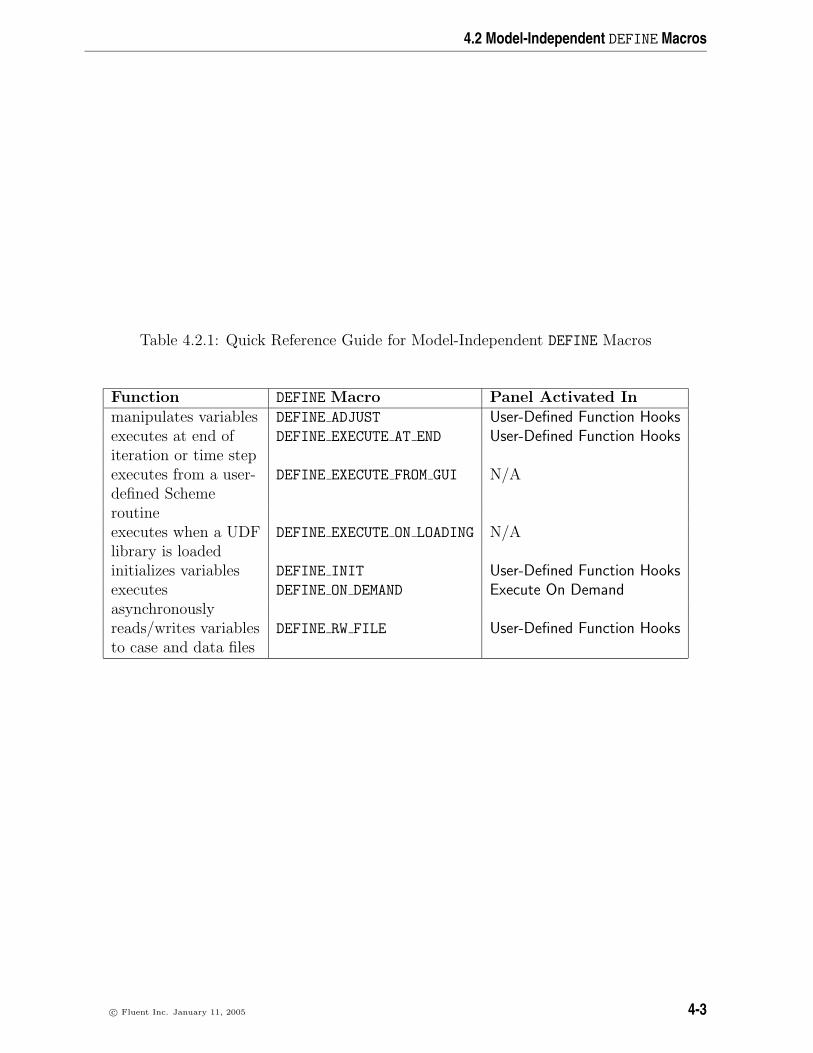
4.2 Model-Independent DEFINE Macros
Table 4.2.1: Quick Reference Guide for Model-Independent DEFINE Macros
Function DEFINE Macro Panel Activated Inmanipulates variables DEFINE ADJUST User-Defined Function Hooksexecutes at end of DEFINE EXECUTE AT END User-Defined Function Hooksiteration or time stepexecutes from a user- DEFINE EXECUTE FROM GUI N/Adefined Schemeroutineexecutes when a UDF DEFINE EXECUTE ON LOADING N/Alibrary is loadedinitializes variables DEFINE INIT User-Defined Function Hooksexecutes DEFINE ON DEMAND Execute On Demandasynchronouslyreads/writes variables DEFINE RW FILE User-Defined Function Hooksto case and data files
c© Fluent Inc. January 11, 2005 4-3

Defining a UDF Using a DEFINE Macro
4.2.1 DEFINE ADJUST
Description
DEFINE ADJUST is a general-purpose macro that can be used to adjust or modify FLUENTvariables that are not passed as arguments. For example, you can use DEFINE ADJUST tomodify flow variables (e.g., velocities, pressure) and compute integrals. You can also useit to integrate a scalar quantity over a domain and adjust a boundary condition based onthe result. A function that is defined using DEFINE ADJUST executes at every iterationand is called at the beginning of every iteration before transport equations are solved.Refer to Figures 1.10.1 and 1.10.2 for an overview of the FLUENT solution process whichshows when a DEFINE ADJUST is called.
Usage
DEFINE ADJUST(name,d)
Argument Type Descriptionchar name UDF name.Domain *d Pointer to the domain over which the adjust function is
to be applied. The domain argument provides access to allcell and face threads in the mesh. For multiphase flows, thepointer that is passed to the function by the solver is themixture-level domain.
Function returnsvoid
There are two arguments to DEFINE ADJUST: name and d. You will supply name, the nameof the UDF. d is passed by the FLUENT solver to your UDF.
4-4 c© Fluent Inc. January 11, 2005

4.2 Model-Independent DEFINE Macros
Example 1
The following UDF, named my adjust, integrates the turbulent dissipation over theentire domain using DEFINE ADJUST. This value is then printed to the console window.The UDF is called once every iteration. It can be executed as an interpreted or compiledUDF in FLUENT.
/********************************************************************
UDF for integrating turbulent dissipation and printing it to
console window
*********************************************************************/
#include "udf.h"
DEFINE_ADJUST(my_adjust,d)
Thread *t;
/* Integrate dissipation. */
real sum_diss=0.;
cell_t c;
thread_loop_c(t,d)
begin_c_loop(c,t)
sum_diss += C_D(c,t)*
C_VOLUME(c,t);
end_c_loop(c,t)
printf("Volume integral of turbulent dissipation: %g\n", sum_diss);
c© Fluent Inc. January 11, 2005 4-5

Defining a UDF Using a DEFINE Macro
Example 2
The following UDF, named adjust fcn, specifies a user-defined scalar as a function ofthe gradient of another user-defined scalar, using DEFINE ADJUST. The function is calledonce every iteration. It is executed as a compiled UDF in FLUENT.
/********************************************************************
UDF for defining user-defined scalars and their gradients
*********************************************************************/
#include "udf.h"
DEFINE_ADJUST(adjust_fcn,d)
Thread *t;
cell_t c;
real K_EL = 1.0;
/* Do nothing if gradient isn’t allocated yet. */
if (! Data_Valid_P())
return;
thread_loop_c(t,d)
if (FLUID_THREAD_P(t))
begin_c_loop_all(c,t)
C_UDSI(c,t,1) +=
K_EL*NV_MAG2(C_UDSI_G(c,t,0))*C_VOLUME(c,t);
end_c_loop_all(c,t)
Hooking an Adjust UDF to FLUENT
After the UDF that you have defined using DEFINE ADJUST is interpreted (Chapter 7: In-terpreting UDF Source Files) or compiled (Chapter 8: Compiling UDF Source Files),the name that you specified in the DEFINE macro argument (e.g., adjust fcn) will be-come visible and selectable in the User-Defined Function Hooks panel in FLUENT. SeeSection 9.1.1: DEFINE ADJUST for details.
4-6 c© Fluent Inc. January 11, 2005

4.2 Model-Independent DEFINE Macros
4.2.2 DEFINE EXECUTE AT END
Description
DEFINE EXECUTE AT END is a general purpose macro that is executed at the end of aniteration in a steady state run, or at the end of a time step in a transient run. Youcan use DEFINE EXECUTE AT END when you want to calculate flow quantities at theseparticular times. Note that you do not have to specify whether your execute-at-endUDF gets executed at the end of a time step or the end of an iteration. This is doneautomatically when you select the steady or unsteady time method in your FLUENTmodel.
Usage
DEFINE EXECUTE AT END(name)
Argument Type Descriptionchar name UDF name.
Function returnsvoid
There is only one argument to DEFINE EXECUTE AT END: name. You will supply name,the name of the UDF. Unlike DEFINE ADJUST, DEFINE EXECUTE AT END is not passed adomain pointer. Therefore, if your function requires access to a domain pointer, then youwill need to use the utility Get Domain(ID) to explicitly obtain it (see Section 6.5.1: Do-main Pointer Using Get Domain and the example below). If your UDF requires access toa phase domain pointer in a multiphase solution, then it will need to pass the appropriatephase ID to Get Domain in order to obtain it.
c© Fluent Inc. January 11, 2005 4-7
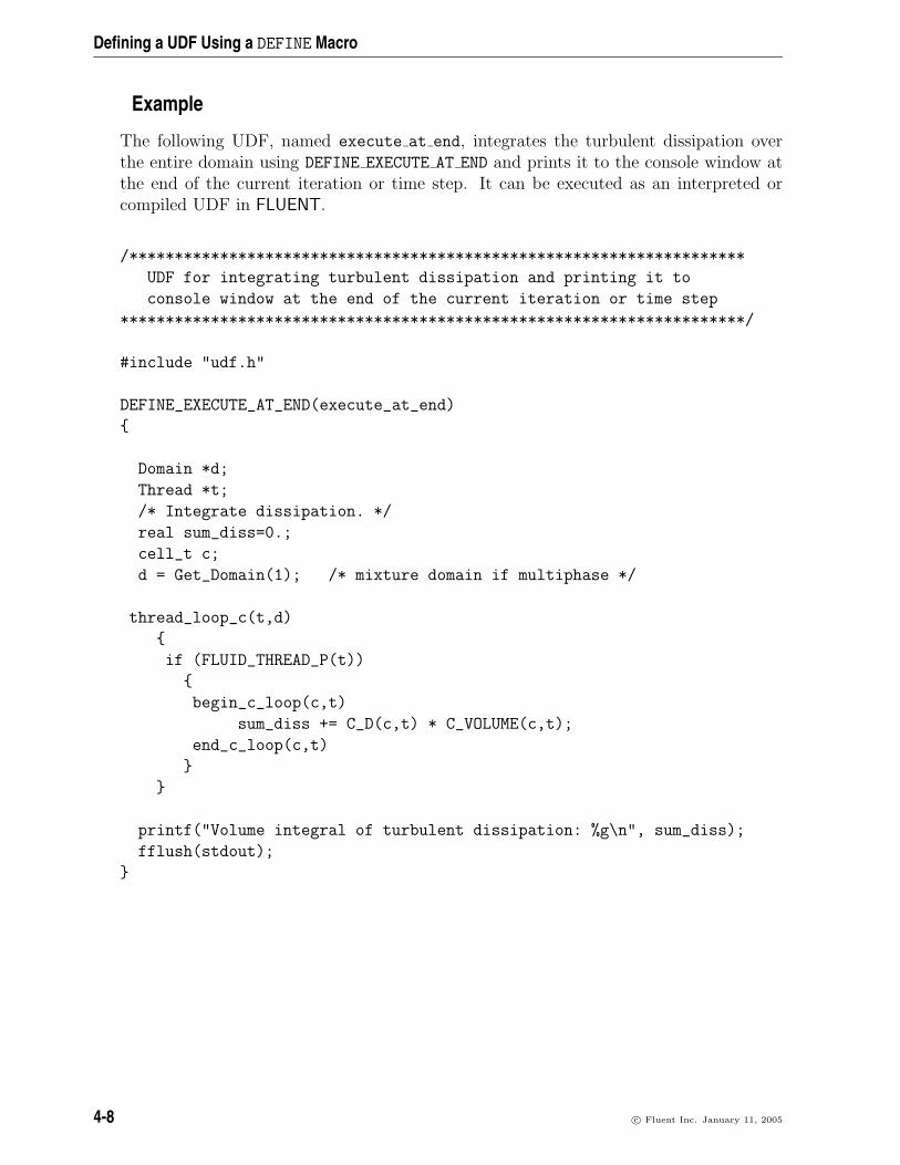
Defining a UDF Using a DEFINE Macro
Example
The following UDF, named execute at end, integrates the turbulent dissipation overthe entire domain using DEFINE EXECUTE AT END and prints it to the console window atthe end of the current iteration or time step. It can be executed as an interpreted orcompiled UDF in FLUENT.
/********************************************************************
UDF for integrating turbulent dissipation and printing it to
console window at the end of the current iteration or time step
*********************************************************************/
#include "udf.h"
DEFINE_EXECUTE_AT_END(execute_at_end)
Domain *d;
Thread *t;
/* Integrate dissipation. */
real sum_diss=0.;
cell_t c;
d = Get_Domain(1); /* mixture domain if multiphase */
thread_loop_c(t,d)
if (FLUID_THREAD_P(t))
begin_c_loop(c,t)
sum_diss += C_D(c,t) * C_VOLUME(c,t);
end_c_loop(c,t)
printf("Volume integral of turbulent dissipation: %g\n", sum_diss);
fflush(stdout);
4-8 c© Fluent Inc. January 11, 2005

4.2 Model-Independent DEFINE Macros
Hooking an Execute-at-End UDF to FLUENT
After the UDF that you have defined using DEFINE EXECUTE AT END is interpreted (Chap-ter 7: Interpreting UDF Source Files) or compiled (Chapter 8: Compiling UDF SourceFiles), the name that you specified in the DEFINE macro argument (e.g. execute at end)will become visible and selectable in the User-Defined Function Hooks panel in FLUENT.See Section 9.1.2: DEFINE EXECUTE AT END for details.
c© Fluent Inc. January 11, 2005 4-9

Defining a UDF Using a DEFINE Macro
4.2.3 DEFINE EXECUTE FROM GUI
Description
You can use DEFINE EXECUTE FROM GUI to define a UDF that is executed from a user-defined graphical user interface (GUI) using the Scheme language. For example, a Cfunction that you define using DEFINE EXECUTE FROM GUI can be executed whenever abutton is clicked in a user-defined GUI.
Usage
DEFINE EXECUTE FROM GUI(name,libname,mode)
Argument Type Descriptionchar name UDF name.char *libname name of the UDF library that has been loaded in FLUENTint mode an integer passed from the Scheme program that defines the
user-defined GUI.
Function returnsvoid
There are three arguments to DEFINE EXECUTE FROM GUI: name, libname, and mode. Youwill supply name, the name of the UDF. The variables libname and mode are passed bythe FLUENT solver to your UDF. The integer variable mode is passed from the Schemeprogram which defines the user-defined GUI, and represent the possible user optionsavailable from the GUI panel. A different C function in UDF can be called for eachoption. For example, the user-defined GUI panel may have a number of buttons. Eachbutton may be represented by different integers, which, when clicked, will execute acorresponding C function.
i DEFINE EXECUTE FROM GUI UDFs must be implemented as compiled UDFs,and there can be only one function of this type in a UDF library.
4-10 c© Fluent Inc. January 11, 2005

4.2 Model-Independent DEFINE Macros
Example
The following UDF, named reset udm, resets all user-defined memory (UDM) valueswhen a reset button on a user-defined GUI panel is clicked. The clicking of the buttonis represented by 0, which is passed to the UDF by the FLUENT solver.
/*********************************************************
UDF called from a user-defined GUI panel to reset all
all user-defined memory locations
**********************************************************/
#include "udf.h"
DEFINE_EXECUTE_FROM_GUI(reset_udm, myudflib, mode)
Domain *domain = Get_Domain(1); /* Get domain pointer */
Thread *t;
cell_t c;
int i;
/* Return if mode is not zero */
if (mode != 0) return;
/* Return if no User-Defined Memory is defined in FLUENT */
if (n_udm == 0) return;
/* Loop over all cell threads in domain */
thread_loop_c(t, domain)
/* Loop over all cells */
begin_c_loop(c, t)
/* Set all UDMs to zero */
for (i = 0; i < n_udm; i++)
C_UDMI(c, t, i) = 0.0;
end_c_loop(c, t);
c© Fluent Inc. January 11, 2005 4-11

Defining a UDF Using a DEFINE Macro
Hooking an Execute From GUI UDF to FLUENT
After the UDF that you have defined using DEFINE EXECUTE FROM GUI is compiled (Chap-ter 8: Compiling UDF Source Files), the function will not need to be hooked to FLUENTthrough any graphics panels. Instead, the function will be searched automatically by theFLUENT solver when the execution of the UDF is requested (i.e., when a call is madefrom a user-defined Scheme program to execute a C function).
4-12 c© Fluent Inc. January 11, 2005

4.2 Model-Independent DEFINE Macros
4.2.4 DEFINE EXECUTE ON LOADING
Description
You can use DEFINE EXECUTE ON LOADING to specify a function that executes as soon asa compiled UDF library is loaded in FLUENT. This is useful when you want to initializeor setup UDF models when a UDF library is loaded. (Alternatively, if you save your casefile when a shared library is loaded, then the UDF will execute whenever the case file issubsequently read.)
Compiled UDF libraries are loaded using either the Compiled UDFs or the UDF LibraryManager panel (see Section 8.5: Load and Unload Libraries Using the UDF Library ManagerPanel). An EXECUTE ON LOADING UDF is the best place to reserve user-defined scalar(UDS) and user-defined memory (UDM) for a particular library (Sections 5.5.3 and 5.6.4)as well as set UDS and UDM names (Sections 5.5.5 and 5.6.6).
i DEFINE EXECUTE ON LOADING UDFs can be executed only as compiledUDFs.
Usage
DEFINE EXECUTE ON LOADING(name,libname)
Argument Type Descriptionchar name UDF name.char *libname compiled UDF library name.
Function returnsvoid
There are two arguments to DEFINE EXECUTE ON LOADING: name and libname. You willsupply a name for the UDF which will be used by FLUENT when reporting that theEXECUTE ON LOADING UDF is being run. The libname is set by FLUENT to be the nameof the library (e.g., libudf) that you have specified (by entering a name or keeping thedefault libudf). libname is passed so that you can use it in messages within your UDF.
c© Fluent Inc. January 11, 2005 4-13

Defining a UDF Using a DEFINE Macro
Example 1
The following simple UDF named report version, prints a message on the console thatcontains the version and release number of the library being loaded.
#include "udf.h"
static int version = 1;
static int release = 2;
DEFINE_EXECUTE_ON_LOADING(report_version, libname)
Message("\nLoading %s version %d.%d\n",libname,version,release);
Example 2
The following source code contains two UDFs. The first UDF is an EXECUTE ON LOADING
function that is used to reserve three UDMs (using Reserve User Memory Vars) for alibrary and set unique names for the UDM locations (using Set User Memory Name). Thesecond UDF is an ON DEMAND function that is used to set the values of the UDM locationsafter the solution has been initialized. The ON DEMAND UDF sets the initial values of theUDM locations using udf offset, which is defined in the on-loading UDF. Note thatthe on demand UDF must be executed after the solution is initialized to reset the initialvalues for the UDMs. See Sections 5.6.4 and 5.6.6 for more information on reserving andnaming UDMs.
/**********************************************************************
udm_res1.c contains two UDFs: an execute on loading UDF that reserves
three UDMs for libudf and renames the UDMs to enhance postprocessing,
and an on-demand UDF that sets the initial value of the UDMs.
**********************************************************************/
#include "udf.h"
#define NUM_UDM 3
static int udm_offset = UDM_UNRESERVED;
DEFINE_EXECUTE_ON_LOADING(on_loading, libname)
if (udm_offset == UDM_UNRESERVED) udm_offset =
Reserve_User_Memory_Vars(NUM_UDM);
if (udm_offset == UDM_UNRESERVED)
4-14 c© Fluent Inc. January 11, 2005

4.2 Model-Independent DEFINE Macros
Message("\nYou need to define up to %d extra UDMs in GUI and
then reload current library %s\n", NUM_UDM, libname);
else
Message("%d UDMs have been reserved by the current
library %s\n",NUM_UDM, libname);
Set_User_Memory_Name(udm_offset,"lib1-UDM-0");
Set_User_Memory_Name(udm_offset+1,"lib1-UDM-1");
Set_User_Memory_Name(udm_offset+2,"lib1-UDM-2");
Message("\nUDM Offset for Current Loaded Library = %d",udm_offset);
DEFINE_ON_DEMAND(set_udms)
Domain *d;
Thread *ct;
cell_t c;
int i;
d=Get_Domain(1);
if(udm_offset != UDM_UNRESERVED)
Message("Setting UDMs\n");
for (i=0;i<NUM_UDM;i++)
thread_loop_c(ct,d)
begin_c_loop(c,ct)
C_UDMI(c,ct,udm_offset+i)=3.0+i/10.0;
end_c_loop(c,ct)
else
Message("UDMs have not yet been reserved for library 1\n");
c© Fluent Inc. January 11, 2005 4-15

Defining a UDF Using a DEFINE Macro
Hooking an Execute On Loading UDF to FLUENT
After the UDF that you have defined using DEFINE EXECUTE ON LOADING is compiled(Chapter 8: Compiling UDF Source Files), the function will not need to be hookedto FLUENT through any graphics panels. Instead, FLUENT searches the newly-loadedlibrary for any UDFs of the type EXECUTE ON LOADING, and will automatically executethem in the order they appear in the library.
4-16 c© Fluent Inc. January 11, 2005

4.2 Model-Independent DEFINE Macros
4.2.5 DEFINE INIT
Description
You can use DEFINE INIT to specify a set of initial values for your solution. DEFINE INIT
accomplishes the same result as patching, but does it in a different way, by means of aUDF. A DEFINE INIT function is executed once per initialization and is called immedi-ately after the default initialization is performed by the solver. Since it is called after theflow field is initialized, it is typically used to set initial values of flow quantities. Refer toFigures 1.10.1 and 1.10.2 for an overview of the FLUENT solution process which depictswhen a DEFINE INIT function is called.
Usage
DEFINE INIT(name,d)
Argument Type Descriptionchar name UDF name.Domain *d Pointer to the domain over which the initialization function is
to be applied. The domain argument provides access to all celland face threads in the mesh. For multiphase flows, the pointerthat is passed to the function by the solver is the mixture-leveldomain.
Function returnsvoid
There are two arguments to DEFINE INIT: name and d. You will supply name, the nameof the UDF. d is passed from the FLUENT solver to your UDF.
Example
The following UDF, named my init func, initializes flow field variables in a solution. Itis executed once, at the beginning of the solution process. The function can be executedas an interpreted or compiled UDF in FLUENT.
c© Fluent Inc. January 11, 2005 4-17

Defining a UDF Using a DEFINE Macro
/***********************************************************************
UDF for initializing flow field variables
************************************************************************/
#include "udf.h"
DEFINE_INIT(my_init_func,d)
cell_t c;
Thread *t;
real xc[ND_ND];
/* loop over all cell threads in the domain */
thread_loop_c(t,d)
/* loop over all cells */
begin_c_loop_all(c,t)
C_CENTROID(xc,c,t);
if (sqrt(ND_SUM(pow(xc[0] - 0.5,2.),
pow(xc[1] - 0.5,2.),
pow(xc[2] - 0.5,2.))) < 0.25)
C_T(c,t) = 400.;
else
C_T(c,t) = 300.;
end_c_loop_all(c,t)
The macro ND SUM(a,b,c) computes the sum of the first two arguments (2D) or allthree arguments (3D). It is useful for writing functions involving vector operations sothat the same function can be used for 2D and 3D. For a 2D case, the third argument isignored. See Chapter 5: Macros for Accessing FLUENT Solver Variables for a descriptionof predefined solver access macros (e.g., C CENTROID) and Chapter 6: UDF Utilities forutility macros (e.g., ND SUM).
4-18 c© Fluent Inc. January 11, 2005

4.2 Model-Independent DEFINE Macros
Hooking an Initialization UDF to FLUENT
After the UDF that you have defined using DEFINE ADJUST is interpreted (Chapter 7: In-terpreting UDF Source Files) or compiled (Chapter 8: Compiling UDF Source Files),the name that you specified in the DEFINE macro argument (e.g., my init func) willbecome visible and selectable in the User-Defined Function Hooks panel in FLUENT. SeeSection 9.1.3: DEFINE INIT for details.
c© Fluent Inc. January 11, 2005 4-19

Defining a UDF Using a DEFINE Macro
4.2.6 DEFINE ON DEMAND
Description
You can use DEFINE ON DEMAND to specify a UDF that you can execute on demand inFLUENT, rather than having FLUENT call it automatically during the calculation. YourUDF will be executed immediately, once it is activated, but it is not accessible whilethe solver is iterating. Note that the domain pointer d is not explicitly passed as anargument to DEFINE ON DEMAND. Therefore, if you want to use the domain variable inyour on-demand function, you will need to first retrieve it using the Get Domain utilityprovided by Fluent (shown in the example below). See Section 6.5.1: Domain PointerUsing Get Domain for details on Get Domain.
Usage
DEFINE ON DEMAND(name)
Argument Type Descriptionchar name UDF name.
Function returnsvoid
There is only one argument to DEFINE ON DEMAND: name. You will supply name, the nameof the UDF.
Example
The following UDF, named on demand calc, computes and prints the minimum, maxi-mum, and average temperatures for the current data field. It then computes a tempera-ture function
f(T ) =T − Tmin
Tmax − Tmin
and stores it in user-defined memory location 0 (which is allocated as described in Sec-tion 5.3: Cell Variables). Once you hook the on-demand UDF (as described in Sec-tion 9.1.4: DEFINE ON DEMAND), the field values for f(T ) will be available in drop-downlists in post-processing panels in FLUENT. You can select this field by choosing UserMemory 0 in the User Defined Memory... category. If you write a data file after executingthe UDF, the user-defined memory field will be saved to the data file. This source codecan be interpreted or compiled in FLUENT.
4-20 c© Fluent Inc. January 11, 2005

4.2 Model-Independent DEFINE Macros
/**********************************************************************
UDF to calculate temperature field function and store in
user-defined memory. Also print min, max, avg temperatures.
***********************************************************************/
#include "udf.h"
DEFINE_ON_DEMAND(on_demand_calc)
Domain *d; /* declare domain pointer since it is not passed as an
argument to the DEFINE macro */
real tavg = 0.;
real tmax = 0.;
real tmin = 0.;
real temp,volume,vol_tot;
Thread *t;
cell_t c;
d = Get_Domain(1); /* Get the domain using Fluent utility */
/* Loop over all cell threads in the domain */
thread_loop_c(t,d)
/* Compute max, min, volume-averaged temperature */
/* Loop over all cells */
begin_c_loop(c,t)
volume = C_VOLUME(c,t); /* get cell volume */
temp = C_T(c,t); /* get cell temperature */
if (temp < tmin || tmin == 0.) tmin = temp;
if (temp > tmax || tmax == 0.) tmax = temp;
vol_tot += volume;
tavg += temp*volume;
end_c_loop(c,t)
tavg /= vol_tot;
printf("\n Tmin = %g Tmax = %g Tavg = %g\n",tmin,tmax,tavg);
c© Fluent Inc. January 11, 2005 4-21

Defining a UDF Using a DEFINE Macro
/* Compute temperature function and store in user-defined memory*/
/*(location index 0) */
begin_c_loop(c,t)
temp = C_T(c,t);
C_UDMI(c,t,0) = (temp-tmin)/(tmax-tmin);
end_c_loop(c,t)
Get Domain is a macro that retrieves the pointer to a domain. It is necessary to getthe domain pointer using this macro since it is not explicitly passed as an argumentto DEFINE ON DEMAND. The function, named on demand calc, does not take any explicitarguments. Within the function body, the variables that are to be used by the function aredefined and initialized first. Following the variable declarations, a looping macro is usedto loop over each cell thread in the domain. Within that loop another loop is used to loopover all the cells. Within the inner loop, the total volume and the minimum, maximum,and volume-averaged temperature are computed. These computed values are printed tothe FLUENT console. Then a second loop over each cell is used to compute the functionf(T ) and store it in user-defined memory location 0. Refer to Chapter 5: Macros forAccessing FLUENT Solver Variables for a description of predefined solver access macros(e.g., C T) and Chapter 6: UDF Utilities for utility macros (e.g., begin c loop).
Hooking an On-Demand UDF to FLUENT
After the UDF that you have defined using DEFINE ON DEMAND is interpreted (Chap-ter 7: Interpreting UDF Source Files) or compiled (Chapter 8: Compiling UDF SourceFiles), the name that you specified in the DEFINE macro argument (e.g., on demand calc)will become visible and selectable in the Execute On Demand panel in FLUENT. See Sec-tion 9.1.4: DEFINE ON DEMAND for details.
4-22 c© Fluent Inc. January 11, 2005

4.2 Model-Independent DEFINE Macros
4.2.7 DEFINE RW FILE
Description
You can use DEFINE RW FILE to specify customized information that you want to bewritten to a case or data file, or read from a case or data file. You can save and re-store custom variables of any data type (e.g., integer, real, CXBoolean, structure) usingDEFINE RW FILE. It is often useful to save dynamic information (e.g., number of occur-rences in conditional sampling) while your solution is being calculated, which is anotheruse of this function. Note that the read order and the write order must be the samewhen you use this function.
Usage
DEFINE RW FILE(name,fp)
Argument Type Descriptionchar name UDF name.FILE *fp Pointer to the file you are reading or writing.
Function returnsvoid
There are two arguments to DEFINE RW FILE: name and fp. You will supply name, thename of the UDF. fp is passed from the solver to the UDF.
i DEFINE RW FILE cannot be used in UDFs that are executed on Windowssystems.
i Do not use the fwrite macro in DEFINE RW FILE functions that are runningon Windows platforms. Use fprintf instead.
c© Fluent Inc. January 11, 2005 4-23

Defining a UDF Using a DEFINE Macro
Example
The following C source code listing contains examples of functions that write informationto a data file and read it back. These functions are concatenated into a single source filethat can be interpreted or compiled in FLUENT.
/***********************************************************************
UDFs that increment a variable, write it to a data file
and read it back in
************************************************************************/
#include "udf.h"
int kount = 0; /* define global variable kount */
DEFINE_ADJUST(demo_calc,d)
kount++;
printf("kount = %d\n",kount);
DEFINE_RW_FILE(writer,fp)
printf("Writing UDF data to data file...\n");
fprintf(fp,"%d",kount); /* write out kount to data file */
DEFINE_RW_FILE(reader,fp)
printf("Reading UDF data from data file...\n");
fscanf(fp,"%d",&kount); /* read kount from data file */
At the top of the listing, the integer kount is defined and initialized to zero. Thefirst function (demo calc) is an ADJUST function that increments the value of kount
at each iteration, since the ADJUST function is called once per iteration. (See Sec-tion 4.2.1: DEFINE ADJUST for more information about ADJUST functions.) The secondfunction (writer) instructs FLUENT to write the current value of kount to the data file,when the data file is saved. The third function (reader) instructs FLUENT to read thevalue of kount from the data file, when the data file is read.
The functions work together as follows. If you run your calculation for, say, 10 iterations(kount has been incremented to a value of 10) and save the data file, then the currentvalue of kount (10) will be written to your data file. If you read the data back intoFLUENT and continue the calculation, kount will start at a value of 10 and will beincremented at each iteration. Note that you can save as many static variables as youwant, but you must be sure to read them in the same order in which they are written.
4-24 c© Fluent Inc. January 11, 2005

4.2 Model-Independent DEFINE Macros
Hooking a Read/Write Case or Data File UDF to FLUENT
After the UDF that you have defined using DEFINE RW FILE is interpreted (Chapter 7: In-terpreting UDF Source Files) or compiled (Chapter 8: Compiling UDF Source Files),the name that you specified in the DEFINE macro argument (e.g., writer) will becomevisible and selectable in the User-Defined Function Hooks panel in FLUENT. See Sec-tion 9.1.5: DEFINE RW FILE for details.
c© Fluent Inc. January 11, 2005 4-25

Defining a UDF Using a DEFINE Macro
4.3 Model-Dependent DEFINE Macros
The DEFINE macros presented in this section are used to set parameters for a particularmodel in FLUENT. Table 4.3 provides a quick reference guide to the DEFINE macros, thefunctions they are used to define, and the panels where they are activated in FLUENT.Definitions of each DEFINE macro are listed in the udf.h header file. For your convenience,they are listed in Appendix A.
• DEFINE CHEM STEP (Section 4.3.1: DEFINE CHEM STEP)
• DEFINE DELTAT (Section 4.3.2: DEFINE DELTAT)
• DEFINE DIFFUSIVITY (Section 4.3.3: DEFINE DIFFUSIVITY)
• DEFINE DOM DIFFUSE REFLECTIVITY (Section 4.3.4: DEFINE DOM DIFFUSE REFLECTIVITY)
• DEFINE DOM SOURCE (Section 4.3.5: DEFINE DOM SOURCE)
• DEFINE DOM SPECULAR REFLECTIVITY (Section 4.3.6: DEFINE DOM SPECULAR REFLECTIVITY)
• DEFINE GRAY BAND ABS COEFF (Section 4.3.7: DEFINE GRAY BAND ABS COEFF)
• DEFINE HEAT FLUX (Section 4.3.8: DEFINE HEAT FLUX)
• DEFINE NET REACTION RATE (Section 4.3.9: DEFINE NET REACTION RATE)
• DEFINE NOX RATE (Section 4.3.10: DEFINE NOX RATE)
• DEFINE PR RATE (Section 4.3.11: DEFINE PR RATE)
• DEFINE PRANDTL (Section 4.3.12: DEFINE PRANDTL)
• DEFINE PROFILE (Section 4.3.13: DEFINE PROFILE)
• DEFINE PROPERTY(Section 4.3.14: DEFINE PROPERTY)
• DEFINE SCAT PHASE FUNC (Section 4.3.15: DEFINE SCAT PHASE FUNC)
• DEFINE SOLAR INTENSITY (Section 4.3.16: DEFINE SOLAR INTENSITY)
• DEFINE SOURCE (Section 4.3.17: DEFINE SOURCE)
• DEFINE SR RATE (Section 4.3.18: DEFINE SR RATE)
• DEFINE TURB PREMIX SOURCE (Section 4.3.19: DEFINE TURB PREMIX SOURCE)
• DEFINE TURBULENT VISCOSITY (Section 4.3.20: DEFINE TURBULENT VISCOSITY)
• DEFINE UDS FLUX (Section 4.3.21: DEFINE UDS FLUX)
• DEFINE UDS UNSTEADY (Section 4.3.22: DEFINE UDS UNSTEADY)
• DEFINE VR RATE (Section 4.3.23: DEFINE VR RATE)
4-26 c© Fluent Inc. January 11, 2005

4.3 Model-Dependent DEFINE Macros
Table 4.3.1: Quick Reference Guide for Model-Dependent DEFINE Functions
Function DEFINE Macro Panel Activated Inhomogeneous net mass DEFINE CHEM STEP User-Defined Functionreaction rate for all Hooksspecies, integrated overa time step
time step size (for time DEFINE DELTAT Iteratedependent solutions)
species or UDS diffusivity DEFINE DIFFUSIVITY Materials
diffusive reflectivity for DEFINE DOM DIFFUSE User-Defined Functiondiscrete ordinates (DO) REFLECTIVITY Hooksmodel
source for DO model DEFINE DOM SOURCE User-Defined FunctionHooks
specular reflectivity for DEFINE DOM SPECULAR User-Defined FunctionDO model REFLECTIVITY Hooks
gray band absorption DEFINE GRAY BAND ABS COEFF Materialscoefficient for DO model
wall heat flux DEFINE HEAT FLUX User-Defined FunctionHooks
homogeneous net mass DEFINE NET REACTION RATE User-Defined Functionreaction rate for all species Hooksall species
NOx formation rates for DEFINE NOX RATE NOx ModelThermal NO, Prompt NO,Fuel NO, and N20Pathways
particle surface reaction DEFINE PR RATE User-Defined Functionrate Hooks
Prandtl numbers DEFINE PRANDTL Viscous Model
c© Fluent Inc. January 11, 2005 4-27

Defining a UDF Using a DEFINE Macro
Table 4.3.2: Quick Reference Guide for Model-Dependent DEFINE Functions- cont.
Function DEFINE Macro Panel Activated Inspecies mass fraction DEFINE PROFILE boundary condition
(e.g., Velocity Inlet)velocity at a boundary DEFINE PROFILE boundary conditionpressure at a boundary DEFINE PROFILE boundary conditiontemperature at a boundary DEFINE PROFILE boundary conditionmass flux at a boundary DEFINE PROFILE boundary conditiontarget mass flow rate for pressure outlet DEFINE PROFILE Pressure Outletturbulence kinetic energy DEFINE PROFILE boundary conditionturbulence dissipation rate DEFINE PROFILE boundary conditionspecific dissipation rate DEFINE PROFILE boundary conditionporosity DEFINE PROFILE boundary conditionviscous resistance DEFINE PROFILE boundary conditioninertial resistance DEFINE PROFILE boundary conditionuser-defined scalar boundary DEFINE PROFILE boundary conditionvalueinternal emissivity DEFINE PROFILE boundary condition
4-28 c© Fluent Inc. January 11, 2005

4.3 Model-Dependent DEFINE Macros
Table 4.3.3: Quick Reference Guide for Model-Dependent DEFINE Functions- cont.
Function DEFINE Macro Panel Activated Inwall thermal conditions DEFINE PROFILE boundary condition(heat flux, heat generation rate,temperature, heat transfer coefficient,external emissivity, external radiationand free stream temperaturewall radiation DEFINE PROFILE boundary condition(internal emissivity, irradiation)wall momentum DEFINE PROFILE boundary condition(shear stress x,y,z componentsswirl component, moving wallvelocity components, roughness height,roughness constant)wall species mass fractions DEFINE PROFILE boundary conditionwall user-defined scalar boundary DEFINE PROFILE boundary conditionvaluewall discrete phase boundary value DEFINE PROFILE boundary condition
c© Fluent Inc. January 11, 2005 4-29

Defining a UDF Using a DEFINE Macro
Table 4.3.4: Quick Reference Guide for Model-Dependent DEFINE Functions- cont.
Function DEFINE Macro Panel Activated Indensity (as function of temperature) DEFINE PROPERTY Materialsdensity (as function of pressure DEFINE PROPERTY Materialsfor compressible liquids)viscosity DEFINE PROPERTY Materialsmass diffusivity DEFINE PROPERTY Materialsthermal conductivity DEFINE PROPERTY Materialsthermal diffusion coefficient DEFINE PROPERTY Materialsabsorption coefficient DEFINE PROPERTY Materialsscattering coefficient DEFINE PROPERTY Materialslaminar flow speed DEFINE PROPERTY Materialsrate of strain DEFINE PROPERTY Materialsspeed of sound function DEFINE PROPERTY Materialsuser-defined mixing law for DEFINE PROPERTY Materialsmixture materials: densityviscosity, thermal conductivityscattering phase function DEFINE SCAT PHASE FUNC Materials
4-30 c© Fluent Inc. January 11, 2005

4.3 Model-Dependent DEFINE Macros
Table 4.3.5: Quick Reference Guide for Model-Dependent DEFINE Functions- cont.
Function DEFINE Macro Panel Activated Insolar intensity DEFINE SOLAR INTENSITY Radiation Modelmass source DEFINE SOURCE boundary conditionmomentum source DEFINE SOURCE boundary conditionenergy source DEFINE SOURCE boundary conditionturbulence kinetic energy DEFINE SOURCE boundary conditionsourceturbulence dissipation rate DEFINE SOURCE boundary conditionsourcespecies mass fraction source DEFINE SOURCE boundary conditionuser-defined scalar source DEFINE SOURCE boundary conditionP1 radiation model source DEFINE SOURCE boundary conditionsurface reaction rate DEFINE SR RATE User-Defined Function(species mass fractions Hooksand site species)turbulent premixed source DEFINE TURB PREMIX SOURCE User-Defined Function
Hooksturbulent viscosity DEFINE TURBULENT VISCOSITY Viscous Modelscalar flux function DEFINE UDS FLUX User-Defined Scalarsscalar unsteady function DEFINE UDS UNSTEADY User-Defined Scalarsvolume reaction rate DEFINE VR RATE User-Defined Function
Hooks
c© Fluent Inc. January 11, 2005 4-31

Defining a UDF Using a DEFINE Macro
Table 4.3.6: Quick Reference Guide for Model-Dependent DEFINE Functions- cont.
Function DEFINE Macro Panel Activated InMULTIPHASE ONLY
volume fraction DEFINE PROFILE boundary condition(all multiphase models)heat transfer coefficient DEFINE PROPERTY Phase Interaction(Eulerian models)surface tension coefficient DEFINE PROPERTY Phase Interaction(VOF model)cavitation surface tension DEFINE PROPERTY Phase Interactioncoefficient (Mixture model)cavitation vaporization DEFINE PROPERTY Phase Interactionpressure (Mixture model)particle or droplet diameter DEFINE PROPERTY Materials(Mixture model)
4-32 c© Fluent Inc. January 11, 2005

4.3 Model-Dependent DEFINE Macros
Table 4.3.7: Quick Reference Guide for Model-Dependent DEFINE Functions- cont.
Function DEFINE Macro Panel Activated InMULTIPHASE ONLY
temperature source DEFINE SOURCE boundary condition(Eulerian, Mixture models)diameter DEFINE PROPERTY Secondary Phase(Eulerian, Mixture models)solids pressure DEFINE PROPERTY Secondary Phase(Eulerian, Mixture models)radial distribution DEFINE PROPERTY Secondary Phase(Eulerian, Mixture models)elasticity modulus DEFINE PROPERTY Secondary Phase(Eulerian, Mixture models)viscosity DEFINE PROPERTY Secondary Phase(Eulerian, Mixture models)temperature DEFINE PROPERTY Secondary Phase(Eulerian, Mixture models)bulk viscosity DEFINE PROPERTY Secondary Phase(Eulerian model)frictional viscosity DEFINE PROPERTY Secondary Phase(Eulerian model)
c© Fluent Inc. January 11, 2005 4-33

Defining a UDF Using a DEFINE Macro
4.3.1 DEFINE CHEM STEP
Description
You can use DEFINE CHEM STEP to compute the homogeneous net mass reaction rate ofall species integrated over a time step:
Y ∆ti = Y 0
i +∫ ∆t
0
dYidtdt (4.3-1)
where Y 0i is the initial mass fraction of species i, t is time, ∆t is the given time step,
and dYidt
is the net mass reaction rate. Y ∆ti is ith species mass fractionat the end of the
integration.
DEFINE CHEM STEP UDFs are used for the EDC and PDF Transport models.
Usage
DEFINE CHEM STEP(name,ifail,n,dt,p,temp,yk)
Argument Type Descriptionchar name UDF name.int *ifail Flag that is set to 0 if the integration was successful, and
otherwise returns a non-zero value.int n Number of volumetric species.real dt Time step.real *p Pointer to pressure.real *temp Pointer to temperature.real *yk Pointer to array of initial species mass fractions.
Function returnsvoid
There are seven arguments to DEFINE CHEM STEP: name, ifail, n, dt, p, temp, and yk.You will supply name, the name of the UDF. ifail, n, dt, p, temp, and yk are variablesthat are passed by the FLUENT solver to your UDF. The output of the function is thearray of mass fractions yk after the integration step. The initial mass fractions in arrayyk are overwritten.
4-34 c© Fluent Inc. January 11, 2005

4.3 Model-Dependent DEFINE Macros
Example
The following UDF, named user chem step, assumes that the net volumetric reactionrate is the expression,
dYkdt
= 1/Nspe − Yk (4.3-2)
where Nspe is the number of species.
An analytic solution exists for the integral of this ODE as,
Y ∆tk = (Y 0
k − 1/Nspe)exp(−∆t) + 1/Nspe (4.3-3)
/***************************************************
Example UDF that demonstrates DEFINE_CHEM_STEP
***************************************************/
#include "udf.h"
DEFINE_CHEM_STEP(user_chem_step,ifail,n,dt,p,temp,yk)
int i;
real c = 1./n_spe, decay = exp(-dt);
for(i=0;i<n_spe;i++)
yk[i] = (yk[i]-c)*decay + c;
Hooking a Chemistry Step UDF to FLUENT
After the UDF that you have defined using DEFINE CHEM STEP is interpreted (Chap-ter 7: Interpreting UDF Source Files) or compiled (Chapter 8: Compiling UDF SourceFiles), the name that you specified in the DEFINE macro argument (e.g., user chem step)will become visible and selectable in the User-Defined Function Hooks panel in FLUENT.See Section 9.2.1: DEFINE CHEM STEP for details.
c© Fluent Inc. January 11, 2005 4-35

Defining a UDF Using a DEFINE Macro
4.3.2 DEFINE DELTAT
Description
You can use DEFINE DELTAT to control the size of the time step during the solutionof a time-dependent problem. Note that this macro can be used only if the adaptivetime-stepping method option has been activated in the Iterate panel in FLUENT.
Usage
DEFINE DELTAT(name,d)
Argument Type Descriptionchar name UDF name.Domain *d Pointer to domain over which the time stepping control
function is to be applied. The domain argument provides accessto all cell and face threads in the mesh. For multiphase flows,the pointer that is passed to the function by the solver is themixture-level domain.
Function returnsreal
There are two arguments to DEFINE DELTAT: name and domain. You will supply name,the name of the UDF. domain is passed by the FLUENT solver to your UDF. Your UDFwill need to compute the real value of the physical time step and return it to the solver.
4-36 c© Fluent Inc. January 11, 2005

4.3 Model-Dependent DEFINE Macros
Example
The following UDF, named mydeltat, is a simple function that shows how you can useDEFINE DELTAT to change the value of the time step in a simulation. First, CURRENT TIME
is used to get the value of the current simulation time (which is assigned to the variableflow time). Then, for the first 0.5 seconds of the calculation, a time step of 0.1 is set.A time step of 0.2 is set for the remainder of the simulation. The time step variableis then returned to the solver. See Section 6.7: Time-Dependent Macros for details onCURRENT TIME.
/*********************************************************************
UDF that changes the time step value for a time-dependent solution
**********************************************************************/
#include "udf.h"
DEFINE_DELTAT(mydeltat,d)
real time_step;
real flow_time = CURRENT_TIME;
if (flow_time < 0.5)
time_step = 0.1;
else
time_step = 0.2;
return time_step;
Hooking an Adaptive Time Step UDF to FLUENT
After the UDF that you have defined using DEFINE DELTAT is interpreted (Chapter 7: In-terpreting UDF Source Files) or compiled (Chapter 8: Compiling UDF Source Files), thename that you specified in the DEFINE macro argument (e.g,. mydeltat) will becomevisible and selectable in the Iterate panel in FLUENT. See Section 9.2.2: DEFINE DELTAT
for details.
c© Fluent Inc. January 11, 2005 4-37

Defining a UDF Using a DEFINE Macro
4.3.3 DEFINE DIFFUSIVITY
Description
You can use DEFINE DIFFUSIVITY to specify the diffusivity for the species transportequations or user-defined scalar (UDS) transport equations.
Usage
DEFINE DIFFUSIVITY(name,c,t,i)
Argument Type Descriptionchar name UDF name.cell t c Cell index.Thread *t Pointer to cell thread on which the diffusivity function is to
be applied.int i Index that identifies the species or user-defined scalar.
Function returnsreal
There are four arguments to DEFINE DIFFUSIVITY: name, c, and t, and i. You will supplyname, the name of the UDF. c, t, and i are variables that are passed by the FLUENTsolver to your UDF. Your UDF will need to compute the diffusivity only for a single celland return the real value to the solver.
Note that diffusivity UDFs are called by FLUENT from within a loop on cell threads.Consequently, your UDF will not need to loop over cells in a thread since FLUENT isdoing it outside of the function call.
4-38 c© Fluent Inc. January 11, 2005
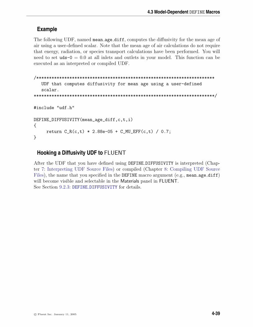
4.3 Model-Dependent DEFINE Macros
Example
The following UDF, named mean age diff, computes the diffusivity for the mean age ofair using a user-defined scalar. Note that the mean age of air calculations do not requirethat energy, radiation, or species transport calculations have been performed. You willneed to set uds-0 = 0.0 at all inlets and outlets in your model. This function can beexecuted as an interpreted or compiled UDF.
/**********************************************************************
UDF that computes diffusivity for mean age using a user-defined
scalar.
***********************************************************************/
#include "udf.h"
DEFINE_DIFFUSIVITY(mean_age_diff,c,t,i)
return C_R(c,t) * 2.88e-05 + C_MU_EFF(c,t) / 0.7;
Hooking a Diffusivity UDF to FLUENT
After the UDF that you have defined using DEFINE DIFFUSIVITY is interpreted (Chap-ter 7: Interpreting UDF Source Files) or compiled (Chapter 8: Compiling UDF SourceFiles), the name that you specified in the DEFINE macro argument (e.g., mean age diff)will become visible and selectable in the Materials panel in FLUENT.See Section 9.2.3: DEFINE DIFFUSIVITY for details.
c© Fluent Inc. January 11, 2005 4-39
Defining a UDF Using a DEFINE Macro
4.3.4 DEFINE DOM DIFFUSE REFLECTIVITY
Description
You can use DEFINE DOM DIFFUSE REFLECTIVITY to modify the inter-facial reflectivitycomputed by FLUENT at diffusely reflecting semi-transparent walls, based on the refrac-tive index values. During execution, a DEFINE DOM DIFFUSE REFLECTIVITY function iscalled by FLUENT for each semi-transparent wall and also for each band (in the case ofa non-gray Discrete Ordinates Model). Therefore the function can be used to modifydiffuse reflectivity and diffuse transmissivity values at the interface.
Usage
DEFINE DOM DIFFUSE REFLECTIVITY(name,t,nb,n a,n b,diff ref a,diff tran a,diff ref b,diff tran b)
i Note that all of the arguments to a DEFINE macro need to be placed on thesame line in your source code. Splitting the DEFINE statement onto severallines will result in a compilation error.
Argument Type Descriptionchar name UDF name.Thread *t Pointer to the thread on which the discrete ordinate
diffusivity function is to be applied.int nb Band number (needed for the non-gray Discrete
Ordinates Model).real n a Refractive index of medium a.real n b Refractive index of medium b.real *diff ref a Diffuse reflectivity at the interface facing medium a.real *diff tran a Diffuse transmissivity at the interface facing medium a.real *diff ref b Diffuse reflectivity at the interface facing medium b.comreal *diff tran b Diffuse transmissivity at the interface facing medium b.
Function returnsvoid
There are nine arguments to DEFINE DOM DIFFUSE REFLECTIVITY: name, t, nb, n a, n b,diff ref a, diff tran a, diff ref b, and diff tran b. You will supply name, the nameof the UDF. t, nb, n a, n b, diff ref a, diff tran a, diff ref b, and diff tran b arevariables that are passed by the FLUENT solver to your UDF.
4-40 c© Fluent Inc. January 11, 2005

4.3 Model-Dependent DEFINE Macros
Example
The following UDF, named user dom diff refl, modifies diffuse reflectivity and trans-missivity values on both the sides of the interface separating medium a and b. The UDFis called for all the semi-transparent walls and prints the value of the diffuse reflectivityand transmissivity values for side a and b.
/* UDF to print the diffuse reflectivity and transmissivity
at semi-transparent walls*/
#include "udf.h"
DEFINE_DOM_DIFFUSE_REFLECTIVITY(user_dom_diff_refl,t,nband,n_a,n_b,
diff_ref_a,diff_tran_a,diff_ref_b,diff_tran_b)
printf("diff_ref_a=%f diff_tran_a=%f \n", *diff_ref_a, *diff_tran_a);
printf("diff_ref_b=%f diff_tran_b=%f \n", *diff_ref_b, *diff_tran_b);
Hooking a Discrete Ordinates Model (DOM) Diffuse Reflectivity UDF toFLUENT
After the UDF that you have defined using DEFINE DOM DIFFUSE REFLECTIVITY is in-terpreted (Chapter 7: Interpreting UDF Source Files) or compiled (Chapter 8: Com-piling UDF Source Files), the name that you specified in the DEFINE macro argument(e.g., user dom diff refl) will become visible and selectable in the User-Defined Func-tion Hooks panel in FLUENT. See Section 9.2.4: DEFINE DOM DIFFUSE REFLECTIVITY fordetails.
c© Fluent Inc. January 11, 2005 4-41

Defining a UDF Using a DEFINE Macro
4.3.5 DEFINE DOM SOURCE
Description
You can use DEFINE DOM SOURCE to modify the emission term (first term on the righthand side of Equation 12.3-37 or Equation 12.3-38 of the User’s Guide manual) as wellas the scattering term (second term on the right hand side of either equation) in theradiative transport equation for the Discrete Ordinates (DO) model.
Usage
DEFINE DOM SOURCE(name,c,t,ni,nb,emission,in scattering,abs coeff,scat coeff)
Argument Type Descriptionchar name UDF name.cell t c Cell index.Thread *t Pointer to cell thread.int ni Direction represented by the solid angle.int nb Band number (needed for the non-gray Discrete Ordinates
Model).real *emission Pointer to emission term in the radiative transport
equation (Equation 12.3-37 of the User’s Guide manual).real *in scattering Pointer to scattering term in the radiative transport
equation (Equation 12.3-38 of the User’s Guide manual).real *abs coeff Pointer to absorption coefficient.real *scat coeff Pointer to scattering coefficient.
Function returnsvoid
There are nine arguments to DEFINE DOM SOURCE: name, c, ni, nb, emission,in scattering, abs coeff, and scat coeff. You will supply name, the name of theUDF. c, ni, nb, emission, in scattering, abs coeff, and scat coeff are variablesthat are passed by the FLUENT solver to your UDF. DEFINE DOM SOURCE is called byFLUENT for each cell.
4-42 c© Fluent Inc. January 11, 2005

4.3 Model-Dependent DEFINE Macros
Example
In the following UDF, named user dom source, the emission term present in the radiativetransport equation is modified. The UDF is called for all the cells and increases theemission term by 5%.
/* UDF to alter the emission source term in the DO model */
#include "udf.h"
DEFINE_DOM_SOURCE(user_dom_source,c,t,ni,nb,emission,in_scattering,
abs_coeff,scat_coeff)
/* increased the emission by 5 % */
*emission *= 1.05;
i Note that all of the arguments to a DEFINE macro need to be placed on thesame line in your source code. Splitting the DEFINE statement onto severallines will result in a compilation error.
Hooking a DOM Source UDF to FLUENT
After the UDF that you have defined using DEFINE DOM SOURCE is interpreted (Chap-ter 7: Interpreting UDF Source Files) or compiled (Chapter 8: Compiling UDF SourceFiles), the name that you specified in the DEFINE macro argument (e.g., user dom source)will become visible and selectable in the User-Defined Function Hooks panel in FLUENT.See Section 9.2.5: DEFINE DOM SOURCE for details.
c© Fluent Inc. January 11, 2005 4-43

Defining a UDF Using a DEFINE Macro
4.3.6 DEFINE DOM SPECULAR REFLECTIVITY
Description
You can use DEFINE DOM SPECULAR REFLECTIVITY to modify the inter-facial reflectivityof specularly reflecting semi-transparent walls. You may wish to do this if the reflectivityis dependent on other conditions that the standard boundary condition doesn’t allowfor. ( See Section 12.3.6: Specular Semi-Transparent Walls of the User’s Guide for moreinformation.) During FLUENT execution, the same UDF is called for all the faces of thesemi-transparent wall, for each of the directions.
Usage
DEFINE DOM SPECULAR REFLECTIVITY(name,f,t,nband,n a,n b,ray direction,en,internal reflection,specular reflectivity,specular transmissivity)
i Note that all of the arguments to a DEFINE macro need to be placed on thesame line in your source code. Splitting the DEFINE statement onto severallines will result in a compilation error.
Argument Type Descriptionchar name UDF name.face t f Face index.Thread *t Pointer to face thread on which the specular
reflectivity function is to be applied.int nband Band number (needed for non-gray Discrete
Ordinates Model).real n a Refractive index of medium a.real n b Refractive index of medium b.real ray direction Direction vector (s) defined
in Equation 12.3-50 of the User’s Guide manual.real en Interface normal vector (n) defined
in Equation 12.3-50 of the User’s Guide manual.int internal reflection Variable used to flag the code that total
internal reflector has occurred.real *specular reflectivity Specular reflectivity for the given direction s.real *specular transmissivity Specular transmissivity for the given direction s.
Function returnsvoid
4-44 c© Fluent Inc. January 11, 2005

4.3 Model-Dependent DEFINE Macros
There are eleven arguments to DEFINE DOM SPECULAR REFLECTIVITY: name, f, t, nband,n a, n b, ray direction, en, internal reflection, specular reflectivity, andspecular transmissivity. You will supply name, the name of the UDF. f,t, nband, n a, n b, ray direction, en, internal reflection, specular reflectivity,and specular transmissivity are variables that are passed by the FLUENT solver toyour UDF.
Example
In the following UDF, named user dom spec refl, specular reflectivity and transmis-sivity values are altered for a given ray direction s at face f.
/* UDF to alter the specular reflectivity and transmissivity, at
semi-transparent walls, along direction s at face f */
#include "udf.h"
DEFINE_DOM_SPECULAR_REFLECTIVITY(user_dom_spec_refl,f,t, nband,n_a,n_b,
ray_direction,en,internal_reflection,specular_reflectivity,
specular_transmissivity)
real angle, cos_theta;
real PI = 3.141592;
cos_theta = NV_DOT(ray_direction, en);
angle = acos(cos_theta);
if (angle >45 && angle < 60)
*specular_reflectivity = 0.3;
*specular_transmissivity = 0.7;
Hooking a Discrete Ordinate Model (DOM) Specular Reflectivity UDF toFLUENT
After the UDF that you have defined using DEFINE DOM SPECULAR REFLECTIVITY is in-terpreted (Chapter 7: Interpreting UDF Source Files) or compiled (Chapter 8: Com-piling UDF Source Files), the name that you specified in the DEFINE macro argument(e.g., user dom spec refl) will become visible and selectable in the User-Defined Func-tion Hooks panel in FLUENT. See Section 9.2.6: DEFINE DOM SPECULAR REFLECTIVITY fordetails.
c© Fluent Inc. January 11, 2005 4-45

Defining a UDF Using a DEFINE Macro
4.3.7 DEFINE GRAY BAND ABS COEFF
Description
You can use DEFINE GRAY BAND ABS COEFF to specify a UDF for the gray band absorptioncoefficient as a function of temperature, that can be used with a non-gray discrete ordinatemodel.
Usage
DEFINE GRAY BAND ABS COEFF(name,c,t,nb)
Argument Type Descriptionchar name UDF name.cell t c Cell index.Thread *t Pointer to cell thread.int nb Band number associated with non-gray model.
Function returnsreal
There are four arguments to DEFINE GRAY BAND ABS COEFF: name, c, t, and nb. Youwill supply name, the name of the UDF. The variables c, t, and nb are passed by theFLUENT solver to your UDF. Your UDF will need to return the real value of the grayband coefficient to the solver.
4-46 c© Fluent Inc. January 11, 2005

4.3 Model-Dependent DEFINE Macros
Example
The following UDF, named user gray band abs, specifies the gray-band absorption co-efficient as a function of temperature that can be used for a non-gray Discrete Ordinatemodel.
#include "udf.h"
DEFINE_GRAY_BAND_ABS_COEFF(user_gray_band_abs,c,t,nb)
real abs_coeff = 0;
real T = C_T(c,t);
switch (nb)
case 0 : abs_coeff = 1.3+0.001*T; break;
case 1 : abs_coeff = 2.7 + 0.005*T; break;
return abs_coeff;
Hooking a Gray Band Coefficient UDF to FLUENT
After the UDF that you have defined using DEFINE GRAY BAND ABS COEFF is interpreted(Chapter 7: Interpreting UDF Source Files) or compiled (Chapter 8: Compiling UDFSource Files), the name that you specified in the DEFINE macro argument(e.g., user gray band abs) will become visible and selectable in the Materials panel forthe Absorption Coefficient. See Section 9.2.7: DEFINE GRAY BAND ABS COEFF for details.
c© Fluent Inc. January 11, 2005 4-47

Defining a UDF Using a DEFINE Macro
4.3.8 DEFINE HEAT FLUX
Description
You can use DEFINE HEAT FLUX to modify the heat flux at a wall. Despite the name,a DEFINE HEAT FLUX UDF is not the means to specify the actual heat flux entering adomain from the outside. To specify this type of heat flux, you would simply use aDEFINE PROFILE function in conjunction with a heat flux thermal boundary condition.In contrast, a DEFINE HEAT FLUX UDF allows you to modify the way in which the de-pendence between the flux entering the domain, and the wall and cell temperatures, ismodeled.
Usage
DEFINE HEAT FLUX(name,f,t,c0,t0,cid,cir)
Argument Type Descriptionchar name UDF name.face t f Index that identifies a wall face.Thread *t Pointer to wall face thread on which heat flux function is
to be applied.cell t c0 Cell index that identifies the cell next to the wall.Thread *t0 Pointer to the adjacent cell’s thread.real cid[] Array of fluid-side diffusive heat transfer
coefficients.real cir[] Array of radiative heat transfer coefficients.
Function returnsvoid
There are seven arguments to DEFINE HEAT FLUX: name, f, t, c0, t0, cid, and cir. Youwill supply name, the name of the UDF. f, t, c0, and t0 are variables that are passed bythe FLUENT solver to your UDF. Arrays cir[] and cid[] contain the linearizations ofthe radiative and diffusive heat fluxes, respectively, computed by FLUENT based on theactivated models. These arrays allow you to modify the heat flux in any way that youchoose. FLUENT computes the heat flux at the wall using these arrays after the call toDEFINE HEAT FLUX, so the total heat flux at the wall will be the currently computed heatflux (based on the activated models) with any modifications as defined by your UDF.
4-48 c© Fluent Inc. January 11, 2005

4.3 Model-Dependent DEFINE Macros
The diffusive heat flux (qid) and radiative heat flux (qir) are computed by FLUENTaccording to the following equations:
qid = cid[0] + cid[1]*C_T(c0,t0) - cid[2]*F_T(f,t) - cid[3]*pow(F_T(f,t),4)
qir = cir[0] + cir[1]*C_T(c0,t0) - cir[2]*F_T(f,t) - cir[3]*pow(F_T(f,t),4)
The sum of qid and qir defines the total heat flux from the fluid to the wall (thisdirection being positive flux), and, from an energy balance at the wall, equals the heatflux of the surroundings (exterior to the domain). Note that heat flux UDFs (definedusing DEFINE HEAT FLUX) are called by FLUENT from within a loop over wall faces.
i In order for the solver to compute C T and F T, the values you supply tocid[1] and cid[2] should never be zero.
Example
Section 12.5.2: Implementing FLUENT’s P-1 Radiation Model provides an example of theP-1 radiation model implementation through a user-defined scalar. An example of theusage of the DEFINE HEAT FLUX macro is included in that implementation.
Hooking a Heat Flux UDF to FLUENT
After the UDF that you have defined using DEFINE HEAT FLUX is interpreted (Chap-ter 7: Interpreting UDF Source Files) or compiled (Chapter 8: Compiling UDF SourceFiles), the name that you specified in the DEFINE macro argument (e.g., heat flux) willbecome visible and selectable in the User-Defined Function Hooks panel in FLUENT. SeeSection 9.2.8: DEFINE HEAT FLUX for details.
c© Fluent Inc. January 11, 2005 4-49

Defining a UDF Using a DEFINE Macro
4.3.9 DEFINE NET REACTION RATE
Description
You can use DEFINE NET REACTION RATE to compute the homogeneous net mass reactionrate of all species. The net mass reaction rate of a species is the sum over all reactionsof the volumetric reaction rate, multiplied by the molecular weight of that species:
dYidt
= Mi
NR∑r=1
Rr (4.3-4)
where Yi is the mass fraction of species i, t is time, Mi is the molecular weight of speciesi, Rr is the molar reaction rate of reaction r, and N R is the total number of reactions.
A DEFINE NET REACTION RATE UDF may be used for the EDC and PDF Transport mod-els, as well as for the surface chemistry model. In contrast, the volumetric UDF functionDEFINE VR RATE and surface UDF function DEFINE SR RATE return the molar rate perreaction. You might want to use DEFINE NET REACTION RATE to link to an external pro-gram that provides reaction rates, such as CHEMKIN.
Usage
DEFINE NET REACTION RATE(name,p,temp,yi,rr,jac)
Argument Type Descriptionchar name UDF name.double *p Pointer to pressure variable.double *temp Pointer to temperature variable.double *yi Pointer to array containing species mass fractions.double *rr Pointer to array containing net mass reaction rates.double *jac Pointer to array of Jacobians.
Function returnsvoid
There are six arguments to DEFINE NET REACTION RATE: name, p, temp, yi, rr, and jac.You will supply name, the name of the UDF. p, temp, yi, rr, and jac are variables thatare passed by the FLUENT solver to your UDF. The outputs of the function are the arrayof net mass reaction rates, rr, and the Jacobian array jac. Note that the Jacobian isonly required for surface chemistry, and is the derivative of the surface net mass reactionrate with respect to the species concentration
This macro allows you to modify the heat flux at the walls that are adjacent to the solid.Since, for solids, only heat conduction is occurring (and is already correctly modeled
4-50 c© Fluent Inc. January 11, 2005

4.3 Model-Dependent DEFINE Macros
by the FLUENT energy equation), any extra heat flux due to this macro could have adetrimental effect. To avoid this, make sure that the UDF either excludes the wallsadjacent to solids or make sure that the UDF only includes the necessary walls adjacentto fluids.
Example
The following UDF, named user net reaction rate, assumes that the net volumetricreaction rate is the expression,
dYidt
= 1/Nspe − Yi (4.3-5)
where Nspe is the number of species.
/***********************************************************
Net Reaction Rate Example UDF
************************************************************/
#include "udf.h"
DEFINE_NET_REACTION_RATE(user_net_reaction_rate,p,temp,yi,rr,jac)
int i;
for(i=0;i<n_spe;i++)
rr[i] = 1./(real)n_spe - yi[i];
Hooking a Net Mass Reaction Rate UDF to FLUENT
After the UDF that you have defined using DEFINE NET REACTION RATE is interpreted(Chapter 7: Interpreting UDF Source Files) or compiled (Chapter 8: Compiling UDFSource Files), the name that you specified in the DEFINE macro argument(e.g., user net reaction rate) will become visible and selectable in the User-DefinedFunction Hooks panel in FLUENT. See Section 9.2.9: DEFINE NET REACTION RATE for de-tails.
c© Fluent Inc. January 11, 2005 4-51

Defining a UDF Using a DEFINE Macro
4.3.10 DEFINE NOX RATE
Description
You can use DEFINE NOX RATE to specify a custom NOx rate for thermal NO, promptNO, fuel NO, and N2O intermediate pathways that can either replace the internally-calculated NOx rate in the source term equation, or be added to the FLUENT rate. Thedefault functionality is to add user-defined rates to the FLUENT-calculated rates. If theReplace with UDF Rate box is checked for a given NOx formation pathway in the NOxModel panel, then the FLUENT-calculated rate for that NOx pathway will not be usedand it will instead be replaced by the NOx rate you have defined in your UDF. Whenyou hook a NOx rate UDF to the graphical interface without checking the Replace withUDF Rate box for a particular pathway, then the user NOx rate will be added to theinternally-calculated rate for the source term calculation.
Note that a single UDF is used to define the different rates for the four NOx pathways:thermal NO, prompt NO, fuel NO, and N20 intermediate. That is, a NOx rate UDF cancontain up to four separate rate functions that are concatenated in a single source filewhich you hook to FLUENT.
Usage
DEFINE NOX RATE(name,c,t,Pollut,NOx)
Argument Type Descriptionchar name UDF name.cell t c Cell index.Thread *t Pointer to cell thread on which the NOx rate
is to be applied.Pollut Parameter *Pollut Pointer to the Pollut structure.NOx Parameter *NOx Pointer to the NOx structure.
Function returnsvoid
There are five arguments to DEFINE NOX RATE: name, c, t, Pollut, and NOx. You willsupply name, the name of the UDF. c, t, Pollut, and NOx are variables that are passedby the FLUENT solver to your function. A DEFINE NOX RATE function does not out-put a value. The calculated NO rates (or other pollutant species rates) are returnedthrough the Pollut structure as the forward rate Pollut->fwdrate) and reverse ratePollut->revrate, respectively.
4-52 c© Fluent Inc. January 11, 2005

4.3 Model-Dependent DEFINE Macros
i The data contained within the NOx structure is specific only to the NOx
model. Alternatively, the Pollut structure contains common data thatare useful for all pollutant species (e.g., species molecular weights, gasphase temperature, density). Note that molecular weight extracted fromthe Pollut structure (i.e., Pollut->spe[i]*mw) has units of kg/kg−mol.
Example
The following compiled UDF, named user nox, exactly reproduces the default FLUENTNOx rates for the prompt NO pathway. Note that this UDF will replace the FLUENTrate only if you select the Replace with UDF option for the prompt NO pathway in theNOx Model panel.
See Section 5.10: NOx Variables for details about NOx macros (e.g., POLLUT EQN, MOLECON,ARRH) that are used in pollutant rate calculations in this UDF.
/******************************************************************
UDF example of User-Defined NOx Rate
If used with the "Replace with UDF Rate" checkbox is activated,
this udf will reproduce exactly the default fluent NOx rate
for the prompt NO pathway.
The flag "Pollut->pollut_io_pdf == IN_PDF" should allways
be used for rates other than that from char N, so that if
requested,the contributions will be pdf integrated. Any
contribution from char must be included within a switch
statement of the form "Pollut->pollut_io_pdf == OUT_PDF".
*******************************************************************/
#include "udf.h"
DEFINE_NOX_RATE(user_nox,c,t,Pollut,NOx)
Pollut->fwdrate = 0.0;
Pollut->revrate = 0.0;
switch (Pollut->pollut_io_pdf)
case IN_PDF:
/*Source terms other than those from char must be included here*/
if (POLLUT_EQN(Pollut) == EQ_NO)
c© Fluent Inc. January 11, 2005 4-53

Defining a UDF Using a DEFINE Macro
/* Prompt NOx */
if (NOx->prompt_nox && NOx->prompt_udf_replace)
real f,rf;
Rate_Const K_PM = 6.4e6, 0.0, 36483.49436;
f = 4.75 + 0.0819*NOx->c_number
- 23.2*NOx->equiv_ratio + 32.0*pow(NOx->equiv_ratio,2.)
- 12.2*pow(NOx->equiv_ratio,3.);
rf = ARRH(Pollut, K_PM);
rf *= pow((Pollut->uni_R*Pollut->temp_m/Pollut->press),
(1+NOx->oxy_order));
rf *= pow(MOLECON(Pollut, O2), NOx->oxy_order);
rf *= MOLECON(Pollut, N2)*MOLECON(Pollut, FUEL);
Pollut->fwdrate += f*rf;
case OUT_PDF:
/* Char contributions that do not go into pdf loop must be
included here */
break;
default:
;
Hooking a NOx Rate UDF to FLUENT
After the UDF that you have defined using DEFINE NOX RATE is interpreted (Chap-ter 7: Interpreting UDF Source Files) or compiled (Chapter 8: Compiling UDF SourceFiles), the name that you specified in the DEFINE macro argument (e.g., user nox) willbecome visible and selectable in the NOx Model panel in FLUENT.See Section 9.2.10: DEFINE NOX RATE for details.
4-54 c© Fluent Inc. January 11, 2005

4.3 Model-Dependent DEFINE Macros
4.3.11 DEFINE PR RATE
Description
You can use DEFINE PR RATE to specify a custom particle surface reaction for the multiplesurface reactions particle model. During FLUENT execution, the same UDF is calledsequentially for all particle surface reactions, so DEFINE PR RATE can be used to definecustom reaction rates for a single reaction, or for multiple reactions. The volumetricand wall surface reactions are not affected by the definition of this macro and will followthe designated rates. Note that a DEFINE PR RATE UDF is not called with the coupledsolution option, so you will need to disable the Coupled Heat Mass Solution option inthe Discrete Phase Model panel when using it. The auxiliary function, zbrent pr rate,which is provided below, can be used when there is no analytical solution for the overallparticle reaction rate.
Usage
DEFINE PR RATE(name,c,t,r,mw,ci,p,sf,dif index,cat index,rr)
Argument Type Descriptionchar name UDF name.cell t c Cell index of current particle.Thread *t Pointer to cell thread for particle.Reaction *r Pointer to data structure that represents the current
reaction.real *mw Pointer to array containing gaseous and surface species
molecular weightsreal *ci Pointer to array containing gas partial pressures.Tracked Particle *p Pointer to Tracked Particle data structure that contains
data related to the particle being tracked.real *sf Pointer to array containing mass fractions of the solid
species in the particle char mass at the current time step.int dif index Diffusion controlled species as defined in the Reactions panel
for the current reaction.int cat index Catalyst species as defined in the Reactions panel
for the current reaction.
real *rr Pointer to array containing particle reaction rate (kgmol/s).
Function returnsvoid
c© Fluent Inc. January 11, 2005 4-55

Defining a UDF Using a DEFINE Macro
There are eleven arguments to DEFINE PR RATE: name, c, t, r, mw, ci, p, sf, dif index,cat index, and rr. You will supply name, the name of the UDF. c, t, r, mw, ci, p, sf,dif index, cat index, and rr are variables that are passed by the FLUENT solver toyour UDF. Your UDF will need to set the value referenced by the real pointer rr to theparticle reaction rate in kgmol/s.
Note that p is an argument to many particle-specific macros defined in Section 5.9: DPMVariables and can be used to obtain information about particle properties. Also note thatthe order in which the solid species mass fractions are stored in array sf is the same asthe order in which the species are defined in the Selected Solid Species list in the Materialspanel, which is opened from the Edit Species names option for the Mixture Material.
DEFINE PR RATE is called by FLUENT every time step during the particle tracking cal-culation. The auxiliary function zbrent pr rate is used when there is no analyticalsolution for the overall particle reaction rate. It uses Brent’s method to find the root ofa function known to lie between x1 and x2. The root will be refined until its accuracyhas reached tolerance tol. This is demonstrated in Example 2.
Auxiliary function
zbrent pr rate (real (*func),(real,real [],int [],cxboolean [],char *,) real
ruser[],int iuser[],
cxboolean buser[],char *cuser,real x1 real x2,real tol,cxboolean *ifail)
Auxiliary function returns: real
Example 1
The following UDF, named user pr rate, specifies a particle reaction rate given byEquation 14.3-9 of the User’s Guide manual, where the effectiveness factor ηr is definedas
ηr = 1− x
where x is the fractional conversion of the particle char mass. In this case, the UDF willbe applied to all surface particle reactions defined in the FLUENT model.
4-56 c© Fluent Inc. January 11, 2005

4.3 Model-Dependent DEFINE Macros
/* UDF of specifying the surface reaction rate of a particle */
#include "udf.h"
#define A1 0.002
#define E1 7.9e7
DEFINE_PR_RATE(user_pr_rate,c,t,r,mw,pp,p,sf,dif_i,cat_i,rr)
/* Argument types
cell_t c
Thread *t
Reaction *r (reaction structure)
real *mw (species molecular weight)
real *pp (gas partial pressures)
Tracked_Particle *p (particle structure)
real *sf (current mass fractions of solid species in
particle char mass)
int dif_i (index of diffusion controlled species)
int cat_i (index of catalyst species)
real *rr (rate of reaction kgmol/s)
*/
real ash_mass =
P_INIT_MASS(p)*(1.-DPM_CHAR_FRACTION(p)-DPM_VOLATILE_FRACTION(p));
real one_minus_conv =
MAX(0.,(P_MASS(p) -ash_mass) / P_INIT_MASS(p)/ DPM_CHAR_FRACTION(p));
real rate = A1*exp(-E1/UNIVERSAL_GAS_CONSTANT/P_T(p));
*rr=-rate*P_DIAM(p)*P_DIAM(p)*M_PI*sf[0]*one_minus_conv;
c© Fluent Inc. January 11, 2005 4-57

Defining a UDF Using a DEFINE Macro
Example 2
The following compiled UDF, named user rate, specifies a particle reaction rate givenby Equation 14.3-4 to Equation 14.3-7 of the User’s Guide manual. The reaction orderon the kinetic rate is 0.9 and the effectiveness factor ηr is defined as
ηr = 1− x
where x is the fractional conversion of the particle char mass. In this case it is necessaryto obtain a numerical solution for the overall surface reaction rate.
This UDF is called only for reaction 2, which means that the default FLUENT solutionwill be used for the rest of the particle surface reactions defined.
/* UDF of specifying the surface reaction rate of a particle,
using a numerical solution */
#include "udf.h"
#define c1 5e-12
#define A1 0.002
#define E1 7.9e7
#define tolerance 1e-4
#define order 0.9
real reaction_rate(real rate, real ruser[], int iuser[], cxboolean buser[],
char *cuser)
return (ruser[2]*pow(MAX(0.,(ruser[0]-rate/ruser[1])),order) -rate);
DEFINE_PR_RATE(user_rate,c,t,r,mw,pp,p,sf,dif_i,cat_i,rr)
if (!strcmp(r->name, "reaction-2"))
cxboolean ifail=FALSE;
real ash_mass =
P_INIT_MASS(p)*(1.-DPM_CHAR_FRACTION(p)-DPM_VOLATILE_FRACTION(p));
real one_minus_conv =
MAX(0.,(P_MASS(p) -ash_mass) / P_INIT_MASS(p)/ DPM_CHAR_FRACTION(p));
4-58 c© Fluent Inc. January 11, 2005

4.3 Model-Dependent DEFINE Macros
real ruser[3];
int iuser[1];
cxboolean buser[1];
char cuser[30];
real ratemin, ratemax, root;
ruser[0] = pp[dif_i];
ruser[1] = MAX(1.E-15, (c1*pow(0.5*(P_T(p)+C_T(c,t)),0.75)/P_DIAM(p)));
ruser[2] = A1*exp(-E1/UNIVERSAL_GAS_CONSTANT/P_T(p));
strcpy(cuser, "reaction-2");
ratemin=0;
ratemax=ruser[1]*pp[dif_i];
/* arguments for auxiliary function zbrent_pr_rate */
root = zbrent_pr_rate(reaction_rate, ruser, iuser, buser, cuser,
ratemin, ratemax, tolerance, &ifail);
if (ifail) root=MAX(1.E-15,ruser[1]);
*rr=-root*P_DIAM(p)*P_DIAM(p)*M_PI*sf[0]*one_minus_conv;
Message("Fail status %d\n", ifail);
Message("Reaction rate for reaction %s : %g\n", cuser, *rr);
In this example, a real function named reaction rate is defined at the top of the UDF.The arguments of reaction rate are real rate, and the pointer arrays real ruser[],integer iuser[], cxboolean buser[], and char *cuser, which must be declared anddefined in the main body of the DEFINE PR RATE function.
Typically, if the particle surface reaction rate is described by
rate = f(ruser[],iuser[],rate)
then the real function (in this example reaction rate) should return
f(ruser[],iuser[],rate) - rate
c© Fluent Inc. January 11, 2005 4-59

Defining a UDF Using a DEFINE Macro
The variables cxboolean buser[] and char *cuser can be used to control the flow ofthe program in cases of complicated rate definitions.
ratemin and ratemax, hold the minimum and maximum possible values of the variablerate, respectively. They define the search interval where the numerical algorithm willsearch for the root of the equation, as defined in the function reaction rate. The valueof reaction rate rr will be refined until an accuracy specified by the value of tolerancetol is reached.
The variable ifail will take the value TRUE if the root of the function has not beenfound.
Hooking a Particle Reaction Rate UDF to FLUENT
After the UDF that you have defined using DEFINE PR RATE is interpreted (Chapter 7: In-terpreting UDF Source Files) or compiled (Chapter 8: Compiling UDF Source Files), thename that you specified in the DEFINE macro argument (e.g., user pr rate) will be-come visible and selectable in the User-Defined Function Hooks panel in FLUENT. SeeSection 9.2.11: DEFINE PR RATE for details.
4-60 c© Fluent Inc. January 11, 2005

4.3 Model-Dependent DEFINE Macros
4.3.12 DEFINE PRANDTL
The following DEFINE macros can be used to specify Prandtl numbers in FLUENT, forsingle-phase flows.
DEFINE PRANDTL D
Description
You can use DEFINE PRANDTL D to specify Prandtl numbers for turbulent dissipation (ε).
Usage
DEFINE PRANDTL D(name,c,t)
Argument Type Descriptionchar name UDF name.cell t c Index of cell on which the Prandtl number function is
to be applied.Thread *t Pointer to cell thread.
Function returnsreal
There are three arguments to DEFINE PRANDTL D: name, c, and t. You will supply name,the name of the UDF. c and t are variables that are passed by the FLUENT solver toyour UDF. Your UDF will need to return the real value for the turbulent dissipationPrandtl number to the solver.
Example
An example of a Prandtl D UDF is provided below in the source listing for DEFINE PRANDTL K.
Hooking a Prandtl Number UDF to FLUENT
After the UDF that you have defined using DEFINE PRANDTL D is interpreted (Chap-ter 7: Interpreting UDF Source Files) or compiled (Chapter 8: Compiling UDF SourceFiles), the name that you specified in the DEFINE macro argument (e.g., user pr d)will become visible and selectable in the Viscous Model panel in FLUENT. See Sec-tion 9.2.12: DEFINE PRANDTL for details.
c© Fluent Inc. January 11, 2005 4-61

Defining a UDF Using a DEFINE Macro
DEFINE PRANDTL K
Description
You can use DEFINE PRANDTL K to specify Prandtl numbers for turbulence kinetic energy(k).
Usage
DEFINE PRANDTL K(name,c,t)
Argument Type Descriptionchar name UDF name.cell t c Index that identifies the cell on which the Prandtl number
function is to be applied.Thread *t Pointer to cell thread.
Function returnsreal
There are three arguments to DEFINE PRANDTL K: name, c, and t. You will supply name,the name of the UDF. c and t are variables that are passed by the FLUENT solver toyour UDF. Your UDF will need to return the real value for the kinetic energy Prandtlnumber to the solver.
Example
The following UDF implements a high-Re version of the RNG model, using the k-ε optionthat is activated in FLUENT.
Three steps are required:
1. Set Cmu, C1eps, and C2eps as in the RNG model.
2. Calculate Prandtl numbers for k and ε using the UDF.
3. Add the -r source term in the ε equation.
In the RNG model, diffusion in k and ε equations appears as
(µ+ µt) ∗ α
4-62 c© Fluent Inc. January 11, 2005

4.3 Model-Dependent DEFINE Macros
while in the standard k-ε model, it is given by
µ+µtPr
.
For the new implementation, a UDF is needed to define a Prandtl number Pr as
Pr =µt
[(µ+ µt) ∗ α− µ]
in order to achieve the same implementation as the original RNG Model.
The following functions (which are concatenated into a single C source code file) demon-strate this usage. Note that the source code must be executed as a compiled UDF.
#include "udf.h"
DEFINE_PRANDTL_K(user_pr_k,c,t)
real pr_k, alpha;
real mu = C_MU_L(c,t);
real mu_t = C_MU_T(c,t);
alpha = rng_alpha(1., mu + mu_t, mu);
pr_k = mu_t/((mu+mu_t)*alpha-mu);
return pr_k;
DEFINE_PRANDTL_D(user_pr_d,c,t)
real pr_d, alpha;
real mu = C_MU_L(c,t);
real mu_t = C_MU_T(c,t);
alpha = rng_alpha(1., mu + mu_t, mu);
pr_d = mu_t/((mu+mu_t)*alpha-mu);
return pr_d;
c© Fluent Inc. January 11, 2005 4-63

Defining a UDF Using a DEFINE Macro
DEFINE_SOURCE(eps_r_source,c,t,dS,eqn)
real con, source;
real mu = C_MU_L(c,t);
real mu_t = C_MU_T(c,t);
real k = C_K(c,t);
real d = C_D(c,t);
real prod = C_PRODUCTION(c,t);
real s = sqrt( prod/(mu+ mu_t) ) ;
real eta = s*k/d;
real eta_0 = 4.38;
real term = mu_t*s*s*s/(1.0 + 0.012*eta*eta*eta);
source = - term * (1. - eta/eta_0);
dS[eqn] = - term/d;
return source;
Hooking a Prandtl Number UDF to FLUENT
After the UDF that you have defined using DEFINE PRANDTL K is interpreted (Chap-ter 7: Interpreting UDF Source Files) or compiled (Chapter 8: Compiling UDF SourceFiles), the name that you specified in the DEFINE macro argument (e.g., user pr k)will become visible and selectable in the Viscous Model panel in FLUENT. See Sec-tion 9.2.12: DEFINE PRANDTL for details.
4-64 c© Fluent Inc. January 11, 2005

4.3 Model-Dependent DEFINE Macros
DEFINE PRANDTL O
Description
You can use DEFINE PRANDTL O to specify Prandtl numbers for specific dissipation (ω inthe k-ω model).
Usage
DEFINE PRANDTL O(name,c,t)
Argument Type Descriptionchar name UDF name.cell t c Index that identifies the cell on which the Prandtl number
function is to be applied.Thread *t Pointer to cell thread.
Function returnsreal
There are three arguments to DEFINE PRANDTL O: name, c, and t. You will supply name,the name of the UDF. c and t are variables that are passed by the FLUENT solver to yourUDF. Your UDF will need to return the real value for the specific dissipation Prandtlnumber to the solver.
c© Fluent Inc. January 11, 2005 4-65

Defining a UDF Using a DEFINE Macro
Example
/* Specifying a Constant Specific Dissipation Prandtl Number */
#include "udf.h"
DEFINE_PRANDTL_O(user_pr_o,c,t)
real pr_o;
pr_o = 2.;
return pr_o;
Hooking a Prandtl Number UDF to FLUENT
After the UDF that you have defined using DEFINE PRANDTL O is interpreted (Chap-ter 7: Interpreting UDF Source Files) or compiled (Chapter 8: Compiling UDF SourceFiles), the name that you specified in the DEFINE macro argument (e.g., user pr o)will become visible and selectable in the Viscous Model panel in FLUENT. See Sec-tion 9.2.12: DEFINE PRANDTL for details.
4-66 c© Fluent Inc. January 11, 2005

4.3 Model-Dependent DEFINE Macros
DEFINE PRANDTL T
Description
You can use DEFINE PRANDTL T to specify Prandtl numbers that appear in the tempera-ture equation diffusion term.
Usage
DEFINE PRANDTL T(name,c,t)
Argument Type Descriptionchar name UDF name.cell t c Index that identifies the cell on which the Prandtl number
function is to be applied.Thread *t Pointer to cell thread.
Function returnsreal
There are three arguments to DEFINE PRANDTL T: name, c, and t. You will supply name,the name of the UDF. c and t are variables that are passed by the FLUENT solver toyour UDF. Your UDF will need to return the real value for the temperature Prandtlnumber to the solver.
c© Fluent Inc. January 11, 2005 4-67

Defining a UDF Using a DEFINE Macro
Example
/* Specifying a Constant Temperature Prandtl Number */
#include "udf.h"
DEFINE_PRANDTL_T(user_pr_t,c,t)
real pr_t;
pr_t = 0.85;
return pr_t;
Hooking a Prandtl Number UDF to FLUENT
After the UDF that you have defined using DEFINE PRANDTL T is interpreted (Chap-ter 7: Interpreting UDF Source Files) or compiled (Chapter 8: Compiling UDF SourceFiles), the name that you specified in the DEFINE macro argument (e.g., user pr t)will become visible and selectable in the Viscous Model panel in FLUENT. See Sec-tion 9.2.12: DEFINE PRANDTL for details.
4-68 c© Fluent Inc. January 11, 2005

4.3 Model-Dependent DEFINE Macros
DEFINE PRANDTL T WALL
Description
You can use DEFINE PRANDTL T WALL to specify Prandtl numbers for thermal wall func-tions.
Usage
DEFINE PRANDTL T WALL(name,c,t)
Argument Type Descriptionchar name UDF name.cell t c Index that identifies the cell on which the Prandtl number
function is to be applied.Thread *t Pointer to cell thread.
Function returnsreal
There are three arguments to DEFINE PRANDTL T WALL: name, c, and t. You will supplyname, the name of the UDF. c and t are variables that are passed by the FLUENT solverto your UDF. Your UDF will need to return the real value for the thermal wall functionPrandtl number to the solver.
c© Fluent Inc. January 11, 2005 4-69

Defining a UDF Using a DEFINE Macro
Example
/*************************************************************
Specifying a constant thermal wall function Prandtl number
********************************************************* **/
#include "udf.h"
DEFINE_PRANDTL_T_WALL(user_pr_t_wall,c,t)
real pr_t_wall;
pr_t_wall = 0.85;
return pr_t_wall;
Hooking a Prandtl Number UDF to FLUENT
After the UDF that you have defined using DEFINE PRANDTL T WALL is interpreted (Chap-ter 7: Interpreting UDF Source Files) or compiled (Chapter 8: Compiling UDF SourceFiles), the name that you specified in the DEFINE macro argument (e.g., user pr t wall)will become visible and selectable in the Viscous Model panel in FLUENT. See Sec-tion 9.2.12: DEFINE PRANDTL for details.
4-70 c© Fluent Inc. January 11, 2005

4.3 Model-Dependent DEFINE Macros
4.3.13 DEFINE PROFILE
Description
You can use DEFINE PROFILE to define a custom boundary profile that varies as a functionof spatial coordinates or time. Some of the variables you can customize at a boundaryare:
• velocity, pressure, temperature, turbulence kinetic energy, turbulence dissipationrate, specific dissipation rate
• mass flux
• target mass flow rate as a function of physical flow time
• species mass fraction (species transport)
• volume fraction (multiphase)
• wall thermal conditions (temperature, heat flux, heat generation rate, heat transfercoefficients, and external emissivity, etc.)
• wall momentum conditions (roughness height, roughness constant)
• wall shear and stress conditions
• porosity, viscous resistance, inertial resistance
• volume fraction (Multiphase only)
Note that DEFINE PROFILE allows you to modify only a single value for wall heat flux.Single values are used in the explicit source term which FLUENT does not linearize. Ifyou want to linearize your source term for wall heat flux and account for conductive andradiative heat transfer separately, you will need to use DEFINE HEAT FLUX to specify yourUDF.
Some examples of boundary profile UDFs are provided below.
Usage
DEFINE PROFILE(name,t,i)
c© Fluent Inc. January 11, 2005 4-71

Defining a UDF Using a DEFINE Macro
Argument Type Descriptionchar name UDF name.Thread *t Pointer to thread on which boundary condition is to be
applied.int i Index that identifies the variable that is to be defined.
i is set when you hook the UDF with a variable in a boundarycondition panel through the graphical user interface. This indexis subsequently passed to your UDF by the FLUENT solverso that your function knows which variable to operate on.
Function returnsvoid
There are three arguments to DEFINE PROFILE: name, t, and i. You will supply name,the name of the UDF. t and i are variables that are passed by the FLUENT solver toyour UDF.
While DEFINE PROFILE is usually used to specify a profile condition on a boundary facezone, it can also be used to specify, or fix, flow variables that are held constant duringcomputation in a cell zone. (See Section 7.27: Fixing the Values of Variables of the User’sGuide for more information on fixing values in a cell zone boundary condition.) For thesecases, the arguments of the macro will change accordingly.
Note that unlike source term and property UDFs, profile UDFs (defined usingDEFINE PROFILE) are not called by FLUENT from within a loop on threads in the bound-ary zone. The solver passes only the pointer to the thread associated with the boundaryzone to the DEFINE PROFILE macro. Your UDF will need to do the work of looping overall of the faces in the thread, computing the face value for the boundary variable, andthen storing the value in memory. Fluent has provided you with a face looping macro toloop over all faces in a thread (begin f loop...). See Chapter 6: UDF Utilities for detailsabout face looping macro utilities.
F PROFILE is typically used along with DEFINE PROFILE and is a predefined macro sup-plied by Fluent. F PROFILE stores a boundary condition in memory for a given face andthread and is nested within the face loop as shown in the examples below. It is importantto note that the index i that is an argument to DEFINE PROFILE is the same argumentto F PROFILE. F PROFILE uses the thread pointer t, face identifier f, and index i to setthe appropriate boundary face value in memory. See Section 6.4: Setting Face VariablesUsing F PROFILE for a description of F PROFILE.
In multiphase cases a DEFINE PROFILE UDF may be called more than once (particularlyif the profile is used in a mixture domain thread). If this needs to be avoided, then addthe prefix MP to the UDF name. The function will then be called only once even if it isused for more than one profile.
4-72 c© Fluent Inc. January 11, 2005

4.3 Model-Dependent DEFINE Macros
Example 1 - Pressure Profile
The following UDF, named pressure profile, generates a parabolic pressure profileaccording to the equation
p(y) = 1.1× 10⁵ − 0.1× 10⁵(
y
0.0745
)2
Note that this UDF assumes that the grid is generated such that the origin is at thegeometric center of the boundary zone to which the UDF is to be applied. y is 0.0 atthe center of the inlet and extends to ±0.0745 at the top and bottom of the inlet. Thesource code can be interpreted or compiled in FLUENT.
/***********************************************************************
UDF for specifying steady-state parabolic pressure profile boundary
profile for a turbine vane
************************************************************************/
#include "udf.h"
DEFINE_PROFILE(pressure_profile,t,i)
real x[ND_ND]; /* this will hold the position vector */
real y;
face_t f;
begin_f_loop(f,t)
F_CENTROID(x,f,t);
y = x[1];
F_PROFILE(f,t,i) = 1.1e5 - y*y/(.0745*.0745)*0.1e5;
end_f_loop(f,t)
The function named pressure profile has two arguments: t and i. t is a pointer tothe face’s thread, and i is an integer that is a numerical label for the variable being setwithin each loop.
Within the function body variable f is declared as a face. A one-dimensional array x
and variable y are declared as real data types. Following the variable declarations, alooping macro is used to loop over each face in the zone to create a profile, or an arrayof data. Within each loop, F CENTROID returns the value of the face centroid (array x)for the face with index f that is on the thread pointed to by t. The y coordinate stored
c© Fluent Inc. January 11, 2005 4-73

Defining a UDF Using a DEFINE Macro
in x[1] is assigned to variable y, and is then used to calculate the pressure. This valueis then assigned to F PROFILE which uses the integer i (passed to it by the solver, basedon your selection of the UDF as the boundary condition for pressure in the Pressure Inletpanel) to set the pressure face value in memory.
Example 2 - Velocity, Turbulent Kinetic Energy, and Turbulent Dissipation RateProfiles
In the following example, DEFINE PROFILE is used to generate profiles for the x velocity,turbulent kinetic energy, and dissipation rate, respectively, for a 2D fully-developed ductflow. Three separate UDFs named x velocity, k profile, and dissip profile aredefined. These functions are concatenated in a single C source file and can be interpretedor compiled in FLUENT.
The 1/7th power law is used to specify the x velocity component:
vx = vx,free
(y
δ
)1/7
A fully-developed profile occurs when δ is one-half the duct height. In this example,the mean x velocity is prescribed and the peak (free-stream) velocity is determined byaveraging across the channel.
The turbulent kinetic energy is assumed to vary linearly from a near-wall value of
knw =u2τ√Cµ
to a free-stream value of
kinf = 0.002u2free
The dissipation rate is given by
ε =C3/4µ (k3/2)
`
where the mixing length ` is the minimum of κy and 0.085δ. (κ is the von Karmanconstant = 0.41.)
The friction velocity and wall shear take the forms:
uτ =√τw/ρ
4-74 c© Fluent Inc. January 11, 2005

4.3 Model-Dependent DEFINE Macros
τw =fρu2
free
2
The friction factor is estimated from the Blasius equation:
f = 0.045
(ufreeδ
ν
)−1/4
/**********************************************************************
Concatenated UDFs for fully-developed turbulent inlet profiles
***********************************************************************/
/*#include "udf.h"*/
#define YMIN 0.0 /* constants */
#define YMAX 0.4064
#define UMEAN 1.0
#define B 1./7.
#define DELOVRH 0.5
#define VISC 1.7894e-05
#define CMU 0.09
#define VKC 0.41
/* profile for x-velocity */
DEFINE_PROFILE(x_velocity,t,i)
real y, del, h, x[ND_ND], ufree; /* variable declarations */
face_t f;
h = YMAX - YMIN;
del = DELOVRH*h;
ufree = UMEAN*(B+1.);
begin_f_loop(f,t)
F_CENTROID(x,f,t);
y = x[1];
c© Fluent Inc. January 11, 2005 4-75

Defining a UDF Using a DEFINE Macro
if (y <= del)
F_PROFILE(f,t,i) = ufree*pow(y/del,B);
else
F_PROFILE(f,t,i) = ufree*pow((h-y)/del,B);
end_f_loop(f,t)
/* profile for kinetic energy */
DEFINE_PROFILE(k_profile,t,i)
real y, del, h, ufree, x[ND_ND];
real ff, utau, knw, kinf;
face_t f;
h = YMAX - YMIN;
del = DELOVRH*h;
ufree = UMEAN*(B+1.);
ff = 0.045/pow(ufree*del/VISC,0.25);
utau=sqrt(ff*pow(ufree,2.)/2.0);
knw=pow(utau,2.)/sqrt(CMU);
kinf=0.002*pow(ufree,2.);
begin_f_loop(f,t)
F_CENTROID(x,f,t);
y=x[1];
if (y <= del)
F_PROFILE(f,t,i)=knw+y/del*(kinf-knw);
else
F_PROFILE(f,t,i)=knw+(h-y)/del*(kinf-knw);
end_f_loop(f,t)
4-76 c© Fluent Inc. January 11, 2005

4.3 Model-Dependent DEFINE Macros
/* profile for dissipation rate */
DEFINE_PROFILE(dissip_profile,t,i)
real y, x[ND_ND], del, h, ufree;
real ff, utau, knw, kinf;
real mix, kay;
face_t f;
h = YMAX - YMIN;
del = DELOVRH*h;
ufree = UMEAN*(B+1.);
ff = 0.045/pow(ufree*del/VISC,0.25);
utau=sqrt(ff*pow(ufree,2.)/2.0);
knw=pow(utau,2.)/sqrt(CMU);
kinf=0.002*pow(ufree,2.);
begin_f_loop(f,t)
F_CENTROID(x,f,t);
y=x[1];
if (y <= del)
kay=knw+y/del*(kinf-knw);
else
kay=knw+(h-y)/del*(kinf-knw);
if (VKC*y < 0.085*del)
mix = VKC*y;
else
mix = 0.085*del;
F_PROFILE(f,t,i)=pow(CMU,0.75)*pow(kay,1.5)/mix;
end_f_loop(f,t)
c© Fluent Inc. January 11, 2005 4-77

Defining a UDF Using a DEFINE Macro
Example 3 - Fixed Velocity UDF
In the following example DEFINE PROFILE is used to fix flow variables that are held con-stant during computation in a cell zone. Three separate UDFs named fixed u, fixed v,and fixed ke are defined in a single C source file. They specify fixed velocities thatsimulate the transient startup of an impeller in an impeller-driven mixing tank. Thephysical impeller is simulated by fixing the velocities and turbulence quantities usingthe fix option in FLUENT. See Section 7.27: Fixing the Values of Variables of the User’sGuide for more information on fixing variables.
/***********************************************************************
Concatenated UDFs for simulating an impeller using fixed velocity
************************************************************************/
#include "udf.h"
#define FLUID_ID 1
#define ua1 -7.1357e-2
#define ua2 54.304
#define ua3 -3.1345e3
#define ua4 4.5578e4
#define ua5 -1.9664e5
#define va1 3.1131e-2
#define va2 -10.313
#define va3 9.5558e2
#define va4 -2.0051e4
#define va5 1.1856e5
#define ka1 2.2723e-2
#define ka2 6.7989
#define ka3 -424.18
#define ka4 9.4615e3
#define ka5 -7.7251e4
#define ka6 1.8410e5
#define da1 -6.5819e-2
#define da2 88.845
#define da3 -5.3731e3
#define da4 1.1643e5
#define da5 -9.1202e5
#define da6 1.9567e6
4-78 c© Fluent Inc. January 11, 2005

4.3 Model-Dependent DEFINE Macros
DEFINE_PROFILE(fixed_u,t,i)
cell_t c;
real x[ND_ND];
real r;
begin_c_loop(c,t)
/* centroid is defined to specify position dependent profiles */
C_CENTROID(x,c,t);
r =x[1];
F_PROFILE(c,t,i) =
ua1+(ua2*r)+(ua3*r*r)+(ua4*r*r*r)+(ua5*r*r*r*r);
end_c_loop(c,t)
DEFINE_PROFILE(fixed_v,t,i)
cell_t c;
real x[ND_ND];
real r;
begin_c_loop(c,t)
/* centroid is defined to specify position dependent profiles*/
C_CENTROID(x,c,t);
r =x[1];
F_PROFILE(c,t,i) =
va1+(va2*r)+(va3*r*r)+(va4*r*r*r)+(va5*r*r*r*r);
end_c_loop(c,t)
c© Fluent Inc. January 11, 2005 4-79

Defining a UDF Using a DEFINE Macro
DEFINE_PROFILE(fixed_ke,t,i)
cell_t c;
real x[ND_ND];
real r;
begin_c_loop(c,t)
/* centroid is defined to specify position dependent profiles*/
C_CENTROID(x,c,t);
r =x[1];
F_PROFILE(c,t,i) =
ka1+(ka2*r)+(ka3*r*r)+(ka4*r*r*r)+(ka5*r*r*r*r)+(ka6*r*r*r*r*r);
end_c_loop(c,t)
Example 4 - Wall Heat Generation Rate Profile
The following UDF, named wallheatgenerate, generates a heat generation rate profilefor a planar conduction wall. Once interpreted or compiled, you can activate this UDFin the Wall boundary condition panel in FLUENT.
/* Wall Heat Generation Rate Profile UDF */
#include "udf.h"
DEFINE_PROFILE(wallheatgenerate,thread,i)
real source = 0.001;
face_t f;
begin_f_loop(f,thread)
F_PROFILE(f,thread,i) = source;
end_f_loop(f,thread)
4-80 c© Fluent Inc. January 11, 2005

4.3 Model-Dependent DEFINE Macros
Example 5 - Viscous Resistance Profile in a Porous Zone
The following UDF, named vis res, generates a viscous resistance profile in a porouszone. Once interpreted or compiled and loaded, you can activate this UDF in the Fluidboundary condition panel in FLUENT.
/* Viscous Resistance Profile UDF in a Porous Zone */
#include "udf.h"
DEFINE_PROFILE(vis_res,t,i)
real x[ND_ND];
real a;
cell_t c;
begin_c_loop(c,t)
C_CENTROID(x,c,t);
if( x[1] < (x[0]-0.01) )
a = 1e9;
else
a = 1.0;
F_PROFILE(c,t,i) = a;
end_c_loop(c,t)
c© Fluent Inc. January 11, 2005 4-81

Defining a UDF Using a DEFINE Macro
Example 6 -Target Mass Flow Rate UDF as a Function of Physical Flow Time
For some unsteady problems, it is desirable that the target mass flow rate be a function ofthe physical flow time. This boundary condition can be applied using a DEFINE PROFILE
UDF. The following UDF, named tm pout2, adjusts the mass flow rate from 1.00kg/sto 1.35kg/s when the physical time step is greater than 0.2 seconds. Once interpretedor compiled, you can activate this UDF in the Pressure Outlet boundary condition panelin FLUENT by selecting the Specify target mass-flow rate option, and then choosing theUDF name from the corresponding drop-down list.
i Note that the mass flow rate profile is a function of time and only oneconstant value should be applied to all zone faces at a given time.
/* UDF for setting target mass flow rate in pressure-outlet */
/* at t<0.2 sec the target mass flow rate set to 1.00 kg/s */
/* when t>0.2 sec the target mass flow rate will change to 1.35 kg/s */
#include "udf.h"
DEFINE_PROFILE(tm_pout2, t, nv)
face_t f ;
real flow_time = RP_Get_Real("flow-time");
if (flow_time < 0.2 )
printf("Time = %f sec. \n",flow_time);
printf("Targeted mass-flow rate set at 1.0 kg/s \n");
begin_f_loop(f,t)
F_PROFILE(f,t,nv) = 1.0 ;
end_f_loop(f,t)
else
printf("Time = %f sec. \n",flow_time);
printf("Targeted mass-flow rate set at 1.35 kg/s \n") ;
begin_f_loop(f,t)
F_PROFILE(f,t,nv) = 1.35 ;
4-82 c© Fluent Inc. January 11, 2005

4.3 Model-Dependent DEFINE Macros
end_f_loop(f,t)
Hooking a Boundary Profile UDF to FLUENT
After the UDF that you have defined using DEFINE PROFILE is interpreted (Chapter 7: In-terpreting UDF Source Files) or compiled (Chapter 8: Compiling UDF Source Files), thename that you specified in the DEFINE macro argument (e.g., vis res) will become vis-ible and selectable in the appropriate boundary condition panel (e.g., the Velocity Inletpanel) in FLUENT. See Section 9.2.13: DEFINE PROFILE for details.
c© Fluent Inc. January 11, 2005 4-83

Defining a UDF Using a DEFINE Macro
4.3.14 DEFINE PROPERTY
Description
You can use DEFINE PROPERTY to specify a custom material property in FLUENT forsingle-phase and multiphase flows. When you are writing a user-defined mixing law UDFfor a mixture material, you will need to use special utilities to access species materialproperties. These are described below. If you want to define a custom mass diffu-sivity property, you must use DEFINE DIFFUSIVITY instead of DEFINE PROPERTY. SeeSection 4.3.3: DEFINE DIFFUSIVITY.
Some of the properties you can customize using DEFINE PROPERTY are:
• density (as a function of temperature)
• viscosity
• thermal conductivity
• mass diffusivity
• thermal diffusion coefficient
• absorption and scattering coefficients
• laminar flow speed
• rate of strain
• user-defined mixing laws for density, viscosity, and thermal conductivity of mixturematerials
i UDFs cannot be used to define specific heat properties; specific heat datacan be accessed only and not modified in FLUENT.
i Note that when you specify a user-defined density function for a compress-ible liquid flow application, you must also include a speed of sound func-tion in your model. Compressible liquid density UDFs can be used in thesegregated solver and for single phase, multiphase mixture and cavitationmodels, only. See the example below for details.
4-84 c© Fluent Inc. January 11, 2005

4.3 Model-Dependent DEFINE Macros
For Multiphase Flows
• surface tension coefficient (VOF model)
• cavitation parameters including surface tension coefficient and vaporization pres-sure (Mixture, cavitation models)
• heat transfer coefficient (Mixture model)
• particle or droplet diameter (Mixture model)
• speed of sound function (Mixture, cavitation models)
• density (as a function of pressure) for compressible liquid flows only (Mixture,cavitation models)
• granular temperature and viscosity (Mixture, Eulerian models)
• granular bulk viscosity (Eulerian model)
• solids pressure (Eulerian, Mixture models)
• diameter (Eulerian, Mixture models)
Usage
DEFINE PROPERTY(name,c,t)
Argument Type Descriptionchar name UDF name.cell t c Cell index.Thread *t Pointer to cell thread on which the property function is to be
applied.
Function returnsreal
There are three arguments to DEFINE PROPERTY: name, c, and t. You will supply name,the name of the UDF. c and t are variables that are passed by the FLUENT solver toyour UDF. Your UDF will need to compute the real property only for a single cell andreturn it to the solver.
Note that like source term UDFs, property UDFs (defined using DEFINE PROPERTY) arecalled by FLUENT from within a loop on cell threads. The solver passes all of the variablesneeded to allow a DEFINE PROPERTY UDF to define a custom material, since propertiesare assigned on a cell basis. Consequently, your UDF will not need to loop over cells ina zone since FLUENT is already doing it.
c© Fluent Inc. January 11, 2005 4-85

Defining a UDF Using a DEFINE Macro
Auxiliary Utilities
Some commonly-used auxiliary utilities for custom property UDFs are described below.They are generic property, MATERIAL PROPERTY, THREAD MATERIAL, andmixture species loop.
generic property is a general purpose function that returns the real value for the givenproperty id for the given thread material. It is defined in prop.h and is used only forspecies properties.
The following Property ID variables are available:
• PROP rho, density
• PROP mu, viscosity
• PROP ktc, thermal conductivity
generic property (name,c,t,prop,id,T)
Argument Type Descriptionchar name Function name.cell t c Cell index.Thread *t Pointer to cell thread on which property function is to be
applied.Property *prop Pointer to property array for the thread material that can be
obtained through the macro MATERIAL PROPERTY(m) See below.Property ID id Property ID of the required property you want to define a
custom mixing law for (e.g., PROP ktc for thermal conductivity).See below for list of variables.
real T Temperature at which the property is to be evaluated (used onlyif a polynomial method is specified).
Function returnsreal
4-86 c© Fluent Inc. January 11, 2005

4.3 Model-Dependent DEFINE Macros
MATERIAL PROPERTY is defined in materials.h and returns a real pointer to the Propertyarray prop for the given material pointer m.
MATERIAL PROPERTY(m)
Argument Type DescriptionMaterial *m Material pointer.
Function returnsreal
THREAD MATERIAL is defined in threads.h and returns real pointer m to the Material
that is associated with the given cell thread t.
i Note that in previous versions of FLUENT, THREAD MATERIAL took twoarguments (t,i), but now only takes one (t).
THREAD MATERIAL(t)
Argument Type DescriptionThread *t Pointer to cell thread.
Function returnsreal
mixture species loop is defined in materials.h and loops over all of the species forthe given mixture material.
mixture species loop (m,sp,i)
Argument Type DescriptionMaterial *m Material pointer.Material *sp Species pointer.int i Species index.
Function returnsreal
c© Fluent Inc. January 11, 2005 4-87

Defining a UDF Using a DEFINE Macro
Example 1 - Temperature-dependent Viscosity Property
The following UDF, named cell viscosity, generates a variable viscosity profile tosimulate solidification. The function is called for every cell in the zone. The viscosity inthe warm (T > 288 K) fluid has a molecular value for the liquid (5.5 ×10⁻³kg/m-s), whilethe viscosity for the cooler region (T < 286 K) has a much larger value (1.0 kg/m-s). Inthe intermediate temperature range (286 K ≤ T ≤ 288 K), the viscosity follows a linearprofile that extends between the two values given above:
µ = 143.2135− 0.49725T (4.3-6)
This model is based on the assumption that as the liquid cools and rapidly becomes moreviscous, its velocity will decrease, thereby simulating solidification. Here, no correctionis made for the energy field to include the latent heat of freezing. The source code canbe interpreted or compiled in FLUENT.
/*********************************************************************
UDF that simulates solidification by specifying a temperature-
dependent viscosity property
**********************************************************************/
#include "udf.h"
DEFINE_PROPERTY(cell_viscosity,c,t)
real mu_lam;
real temp = C_T(c,t);
if (temp > 288.)
mu_lam = 5.5e-3;
else if (temp > 286.)
mu_lam = 143.2135 - 0.49725 * temp;
else
mu_lam = 1.;
return mu_lam;
The function cell viscosity is defined on a cell. Two real variables are introduced:temp, the value of C T(c,t), and mu lam, the laminar viscosity computed by the function.The value of the temperature is checked, and based upon the range into which it falls,the appropriate value of mu lam is computed. At the end of the function the computedvalue for the viscosity (mu lam) is returned to the solver.
4-88 c© Fluent Inc. January 11, 2005

4.3 Model-Dependent DEFINE Macros
Example 2 - User-defined Mixing Law for Thermal Conductivity
You can use DEFINE PROPERTY to define custom user-defined mixing laws for density,viscosity, and conductivity of mixture materials. In order to access species materialproperties your UDF will need to utilize auxiliary utilities that are described above.
The following UDF, named mass wtd k, is an example of a mass-fraction weighted con-ductivity function. The UDF utilizes the generic property function to obtain propertiesof individual species. It also makes use of MATERIAL PROPERTY and THREAD MATERIAL.
/*********************************************************************
UDF that specifies a custom mass-fraction weighted conductivity
**********************************************************************/
#include "udf.h"
DEFINE_PROPERTY(mass_wtd_k,c,t)
real sum = 0.; int i;
Material *sp;
real ktc;
Property *prop;
mixture_species_loop(THREAD_MATERIAL(t),sp,i)
prop = (MATERIAL_PROPERTY(sp));
ktc = generic_property(c,t,prop,PROP_ktc,C_T(c,t));
sum += C_YI(c,t,i)*ktc;
return sum;
c© Fluent Inc. January 11, 2005 4-89

Defining a UDF Using a DEFINE Macro
Example 3 - Surface Tension Coefficient UDF
DEFINE PROPERTY can also be used to define a surface tension coefficient UDF for themultiphase VOF model. The following UDF specifies a surface tension coefficient as aquadratic function of temperature. The source code can be interpreted or compiled inFLUENT.
/***************************************************************
Surface Tension Coefficient UDF for the multiphase VOF Model
***************************************************************/
#include "udf.h"
DEFINE_PROPERTY(sfc,c,t)
real T = C_T(c,t);
return 1.35 - 0.004*T + 5.0e-6*T*T;
i Note that surface tension UDFs for the VOF and Mixture multiphase mod-els are both hooked to FLUENT in the Phase Interaction panel, but in differ-ent ways. For the VOF model, the function hook is located in the SurfaceTension tab in the panel. For the Mixture model, however, the functionhook is located in the Mass tab, and will become visible upon selecting theCavitation option.
4-90 c© Fluent Inc. January 11, 2005

4.3 Model-Dependent DEFINE Macros
Example 4 - Density Function for Compressible Liquids
Liquid density is not a constant but is instead a function of the pressure field. In order tostabilize the pressure solution for compressible flows in FLUENT, an extra term relatedto the speed of sound is needed in the pressure correction equation. Consequently, whenyou want to define a custom density function for a compressible flow, your model mustalso include a speed of sound function. Although you can direct FLUENT to calculate aspeed of sound function by choosing one of the available methods (e.g., piecewise-linear,polynomial) in the Materials panel, as a general guideline you should define a speed ofsound function along with your density UDF using the formulation:
√(∂p
∂ρ)
For simplicity, it is recommended that you concatenate the density and speed of soundfunctions into a single UDF source file.
The following UDF source code example contains two concatenated functions: a densityfunction named superfluid density that is defined in terms of pressure and a customspeed of sound function named sound speed.
/********************************************************************
Density UDF for compressible liquid flows
For use with segregated solver, for single phase, multiphase mixture
or cavitation models only.
*********************************************************************/
#include "udf.h"
#define BMODULUS 2.2e9
#define rho_ref 1000.0
DEFINE_PROPERTY(superfluid_density,c,t)
real rho;
real p, dp;
real p_operating;
p_operating = RP_Get_Real("operating-pressure");
p = C_P(c,t);
dp = p-p_operating;
rho = rho_ref/(1.0-dp/BMODULUS);
return rho;
c© Fluent Inc. January 11, 2005 4-91

Defining a UDF Using a DEFINE Macro
DEFINE_PROPERTY(sound_speed,c,t)
real a;
real p, dp,p_operating;
p_operating = RP_Get_Real ("operating-pressure");
p = C_P(c,t);
dp = p-p_operating;
a = (1.-dp/BMODULUS)*sqrt(BMODULUS/rho_ref);
return a;
Hooking a Property UDF to FLUENT
After the UDF that you have defined using DEFINE PROPERTY is interpreted (Chap-ter 7: Interpreting UDF Source Files) or compiled (Chapter 8: Compiling UDF SourceFiles), the name that you specified in the DEFINE macro argument (e.g., sound speed)will become visible and selectable in graphics panels in FLUENT.See Section 9.2.14: DEFINE PROPERTY for details.
4-92 c© Fluent Inc. January 11, 2005

4.3 Model-Dependent DEFINE Macros
4.3.15 DEFINE SCAT PHASE FUNC
Description
You can use DEFINE SCAT PHASE FUNC to specify the radiation scattering phase functionfor the Discrete Ordinates (DO) model. The function computes two values: the fractionof radiation energy scattered from direction i to direction j, and the forward scatteringfactor.
Usage
DEFINE SCAT PHASE FUNC(name,cosine,f)
Argument Type Descriptionchar name UDF name.real cosine Cosine of the angle between directions i and j.real *f Pointer to the location in memory where the real forward
scattering factor is stored.
Function returnsreal
There are three arguments to DEFINE SCAT PHASE FUNC: name, cosine, and f. You willsupply name, the name of the UDF. cosine and f are variables that are passed bythe FLUENT solver to your UDF. Your UDF will need to compute the real fraction ofradiation energy scattered from direction i to direction j and return it to the solver. Notethat the solver computes and stores a scattering matrix for each material by calling thisfunction for each unique pair of discrete ordinates.
c© Fluent Inc. January 11, 2005 4-93

Defining a UDF Using a DEFINE Macro
Example
In the following example, a number of UDFs are concatenated in a single C source file.These UDFs implement backward and forward scattering phase functions that are citedby Jendoubi et al. [1]. The source code can be interpreted or compiled in FLUENT.
/*******************************************************************
UDFs that implement backward and forward scattering
phase functions as cited by Jendoubi et. al.
********************************************************************/
#include "udf.h"
DEFINE_SCAT_PHASE_FUNC(ScatPhiB2,c,fsf)
real phi=0;
*fsf = 0;
phi = 1.0 - 1.2*c + 0.25*(3*c*c-1);
return (phi);
DEFINE_SCAT_PHASE_FUNC(ScatPhiB1,c,fsf)
real phi=0;
*fsf = 0;
phi = 1.0 - 0.56524*c + 0.29783*0.5*(3*c*c-1) +
0.08571*0.5*(5*c*c*c-3*c) + 0.01003/8*(35*c*c*c*c-30*c*c+3) +
0.00063/8*(63*c*c*c*c*c-70*c*c*c+15*c);
return (phi);
DEFINE_SCAT_PHASE_FUNC(ScatPhiF3,c,fsf)
real phi=0;
*fsf = 0;
phi = 1.0 + 1.2*c + 0.25*(3*c*c-1);
return (phi);
4-94 c© Fluent Inc. January 11, 2005

4.3 Model-Dependent DEFINE Macros
DEFINE_SCAT_PHASE_FUNC(ScatPhiF2,c,fsf)
real phi=0;
real coeffs[9]=1,2.00917,1.56339,0.67407,0.22215,0.04725,
0.00671,0.00068,0.00005;
real P[9];
int i;
*fsf = 0;
P[0] = 1;
P[1] = c;
phi = P[0]*coeffs[0] + P[1]*coeffs[1];
for(i=1;i<7;i++)
P[i+1] = 1/(i+1.0)*((2*i+1)*c*P[i] - i*P[i-1]);
phi += coeffs[i+1]*P[i+1];
return (phi);
DEFINE_SCAT_PHASE_FUNC(ScatIso,c,fsf)
*fsf=0;
return (1.0);
Hooking a Scattering Phase UDF to FLUENT
After the UDF that you have defined using DEFINE SCAT PHASE FUNCTION is interpreted(Chapter 7: Interpreting UDF Source Files) or compiled (Chapter 8: Compiling UDFSource Files), the name that you specified in the DEFINE macro argument (e.g., ScatPhiB)will become visible and selectable in the Materials panel in FLUENT.See Section 9.2.14: DEFINE PROPERTY for details.
c© Fluent Inc. January 11, 2005 4-95

Defining a UDF Using a DEFINE Macro
4.3.16 DEFINE SOLAR INTENSITY
Description
You can use the DEFINE SOLAR INTENSITY macro to define direct solar intensity or diffusesolar intensity UDFs for the solar load model. See Chapter 12: Modeling Heat Transferof the User’s Guide for more information on the solar load model.
i Note that solar intensity UDFs are used with the Solar Model, which isavailable only for the 3d geometries in FLUENT.
Usage
DEFINE SOLAR INTENSITY(name,sum x,sun y,sun z,S hour,S minute)
Argument Type Descriptionchar name UDF name.real sun x x component of the sun direction vector.real sun y y component of the sun direction vector.real sun z z component of the sun direction vector.real S hour Time in hours.real S minute Time in minutes.
Function returnsreal
There are six arguments to DEFINE SOLAR INTENSITY: name, sun x, sun y, sun z, S hour,and S minute. You provide the name of your user-defined function. The variables sun x,sun y, sun z, S hour, and S minute are passed by the FLUENT solver to your UDF.Your UDF will need to compute the direct or diffuse solar irradiation and return thereal value (in w/m2) to the solver.
4-96 c© Fluent Inc. January 11, 2005

4.3 Model-Dependent DEFINE Macros
Example
The following source code contains two UDFs: sol direct intensity computes thedirect solar irradiation and returns it to the FLUENT solver, and sol diffuse intensity
computes the diffuse solar irradiation.
#include "udf.h"
DEFINE_SOLAR_INTENSITY(sol_direct_intensity,sun_x,sun_y,sun_z,hour,minute)
real intensity;
intensity = 1019;
printf("solar-time=%f intensity=%e\n", minute, intensity);
return intensity;
DEFINE_SOLAR_INTENSITY(sol_diffuse_intensity,sun_x,sun_y,sun_z,hour,minute)
real intensity;
intensity = 275;
printf("solar-time=%f intensity-diff=%e\n", minute, intensity);
return intensity;
Hooking a Solar Intensity UDF to FLUENT
After the UDF that you have defined using DEFINE SOLAR INTENSITY is interpreted(Chapter 7: Interpreting UDF Source Files) or compiled (Chapter 8: Compiling UDFSource Files), the name that you specified (e.g., sol direct intensity) in the DEFINE
macro argument will become visible and selectable for Direct Solar Irradiation and DiffuseSolar Irradiation in the Radiation Model panel in FLUENT. Note that the solar load modelmust be enabled. See Section 9.2.16: DEFINE SOLAR INTENSITY for details.
c© Fluent Inc. January 11, 2005 4-97

Defining a UDF Using a DEFINE Macro
4.3.17 DEFINE SOURCE
Description
You can use DEFINE SOURCE to specify custom source terms for the different types ofsolved transport equations in FLUENT (except the discrete ordinates radiation model)including:
• mass
• momentum
• k, ε
• energy (also for solid zones)
• species mass fractions
• P1 radiation model
• user-defined scalar (UDS) transport
• granular temperature (Eulerian, Mixture multiphase models)
Usage
DEFINE SOURCE(name,c,t,dS,eqn)
Argument Type Descriptionchar name UDF name.cell t c Index that identifies cell on which the source term is to be applied.Thread *t Pointer to cell thread.real dS[] Array that contains the derivative of the source term with respect
to the dependent variable of the transport equation.int eqn Equation number.
Function returnsreal
There are five arguments to DEFINE SOURCE: name, c, t, dS, and eqn. You will supplyname, the name of the UDF. c, t, dS, and eqn are variables that are passed by theFLUENT solver to your UDF. Note that the source term derivatives may be used tolinearize the source term if they enhance the stability of the solver. To illustrate this,note that the source term can be expressed, in general, as Equation 4.3-7, where φ is thedependent variable, A is the explicit part of the source term, and Bφ is the implicit part.
4-98 c© Fluent Inc. January 11, 2005

4.3 Model-Dependent DEFINE Macros
Sφ = A+Bφ (4.3-7)
Specifying a value for B in Equation 4.3-7 can enhance the stability of the solution andhelp convergence rates due to the increase in diagonal terms on the solution matrix.FLUENT automatically determines if the value of B that is given by the user will aidstability. If it does, then FLUENT will define A as S∗− (∂S/∂φ)∗φ∗, and B as (∂S/∂φ)∗.If not, the source term is handled explicitly.
Your UDF will need to compute the real source term only for a single cell and returnthe value to the solver, but you have the choice of setting the implicit term dS[eqn] todS/dφ, or forcing the explicit solution of the source term by setting it equal to 0.0.
Note that like property UDFs, source term UDFs (defined using DEFINE SOURCE) arecalled by FLUENT from within a loop on cell threads. The solver passes to theDEFINE SOURCE term UDF all the necessary variables it needs to define a custom sourceterm, since source terms are solved on a cell basis. Consequently, your UDF will not needto loop over cells in the thread since FLUENT is already doing it.
The units on all source terms are of the form generation-rate/volume. For example, asource term for the continuity equation would have units of kg/m3-s.
c© Fluent Inc. January 11, 2005 4-99

Defining a UDF Using a DEFINE Macro
Example
The following UDF, named xmom source, is used to add source terms in FLUENT. Thesource code can be interpreted or compiled. The function generates an x-momentumsource term that varies with y position as
source = −0.5C2ρy|vx|vx
Suppose
source = S = −A|vx|vx
where
A = 0.5C2ρy
Then
dS
dvx= −A|vx| − Avx
d
dvx(|vx|)
The source term returned is
source = −A|vx|vx
and the derivative of the source term with respect to vx (true for both positive andnegative values of vx) is
dS
dvx= −2A|vx|
4-100 c© Fluent Inc. January 11, 2005

4.3 Model-Dependent DEFINE Macros
/*******************************************************************/
/* UDF for specifying an x-momentum source term in a spatially */
/* dependent porous media */
/*******************************************************************/
#include "udf.h"
#define C2 100.0
DEFINE_SOURCE(xmom_source,c,t,dS,eqn)
real x[ND_ND];
real con, source;
C_CENTROID(x,c,t);
con = C2*0.5*C_R(c,t)*x[1];
source = -con*fabs(C_U(c, t))*C_U(c,t);
dS[eqn] = -2.*con*fabs(C_U(c,t));
return source;
Hooking a Source UDF to FLUENT
After the UDF that you have defined using DEFINE SOURCE is interpreted (Chapter 7: In-terpreting UDF Source Files) or compiled (Chapter 8: Compiling UDF Source Files), thename that you specified in the DEFINE macro argument (e.g., xmom source) will becomevisible and selectable in the Fluid or Solid boundary condition panel in FLUENT. SeeSection 9.2.17: DEFINE SOURCE for details.
c© Fluent Inc. January 11, 2005 4-101

Defining a UDF Using a DEFINE Macro
4.3.18 DEFINE SR RATE
Description
You can use DEFINE SR RATE to specify a custom surface reaction rate. A custom surfacereaction rate function defined using this macro will overwrite the default reaction rate(e.g., finite-rate) that is specified in the Materials panel. An example of a reactionrate that depends upon gas species mass fractions is provided below. Also provided is areaction rate UDF that takes into account site species.
i Note that the three types of surface reaction species are internally num-bered with an (integer) index i in order
Usage
DEFINE SR RATE(name,f,t,r,my,yi,rr)
Argument Type Descriptionchar name UDF name.face t f Index that identifies a face within the given thread (or cell in
the case of surface reaction in a porous zone).Thread *t Pointer to face thread on which the surface rate reaction is to
be applied.Reaction *r Pointer to data structure for the reaction.real *mw Pointer to array of species molecular weights.real *yi Pointer to array of mass fractions of gas species
at the surface and the coverage of site species (or site fractions).real *rr Pointer to reaction rate.
Function returnsvoid
There are seven arguments to DEFINE SR RATE: name, f, t, r, my, yi, and rr. You willsupply name, the name of the UDF. Once your UDF is compiled and linked, the namethat you have chosen for your function will become visible and selectable in the graphicaluser interface in FLUENT. f, t, r, my, and yi are variables that are passed by the FLUENTsolver to your UDF. Your UDF will need to set the reaction rate to the value referencedby the real pointer rr as shown in the examples below.
4-102 c© Fluent Inc. January 11, 2005

4.3 Model-Dependent DEFINE Macros
Example 1 - Surface Reaction Rate Using Species Mass Fractions
The following compiled UDF, named arrhenius, defines a custom surface reaction rateusing species mass fractions in FLUENT.
/*******************************************************************
Custom surface reaction rate UDF
********************************************************************/
#include "udf.h"
/* ARRHENIUS CONSTANTS */
#define PRE_EXP 1e+15
#define ACTIVE 1e+08
#define BETA 0.0
real arrhenius_rate(real temp)
return
PRE_EXP*pow(temp,BETA)*exp(-ACTIVE/(UNIVERSAL_GAS_CONSTANT*temp));
/* Species numbers. Must match order in Fluent panel */
#define HF 0
#define WF6 1
#define H2O 2
#define NUM_SPECS 3
/* Reaction Exponents */
#define HF_EXP 2.0
#define WF6_EXP 0.0
#define H2O_EXP 0.0
#define MW_H2 2.0
#define STOIC_H2 3.0
c© Fluent Inc. January 11, 2005 4-103

Defining a UDF Using a DEFINE Macro
/* Reaction Rate Routine that is used in both UDFs */
real reaction_rate(cell_t c, Thread *cthread,real mw[],real yi[])
*/ Note that all arguments in the reaction_rate function
call in your .c source file MUST be on the same line or a
compilation error will occur */
real concenHF = C_R(c,cthread)*yi[HF]/mw[HF];
return arrhenius_rate(C_T(c,cthread))*pow(concenHF,HF_EXP);
DEFINE_SR_RATE(arrhenius,f,fthread,r,mw,yi,rr)
*rr =
reaction_rate(F_C0(f,fthread),THREAD_T0(fthread),mw,yi);
real contact_area(cell_t c,Thread *t,int s_id,int *n)
int i = 0;
real area = 0.0, A[ND_ND];
*n = 0;
c_face_loop(c,t,i)
if(THREAD_ID(C_FACE_THREAD(c,t,i)) == s_id)
(*n)++;
F_AREA(A,C_FACE(c,t,i), C_FACE_THREAD(c,t,i));
area += NV_MAG(A);
return area;
4-104 c© Fluent Inc. January 11, 2005

4.3 Model-Dependent DEFINE Macros
Example 2 - Surface Reaction Rate Using Site Species
The following compiled UDF, named my rate, defines a custom surface reaction rate thattakes into account site species.
/*******************************************************************
Custom surface reaction rate UDF
********************************************************************/
#include "udf.h"
/* ARRHENIUS CONSTANTS */
#define PRE_EXP 1e+15
#define ACTIVE 1e+08
#define BETA 0.0
real arrhenius_rate(real temp)
return
PRE_EXP*pow(temp,BETA)*exp(-ACTIVE/(UNIVERSAL_GAS_CONSTANT*temp));
/* Species numbers. Must match order in Fluent panel */
#define HF 0
#define WF6 1
#define H2O 2
#define NUM_SPECS 3
/* Reaction Exponents */
#define HF_EXP 2.0
#define WF6_EXP 0.0
#define H2O_EXP 0.0
#define MW_H2 2.0
#define STOIC_H2 3.0
c© Fluent Inc. January 11, 2005 4-105

Defining a UDF Using a DEFINE Macro
/* Reaction Rate Routine that is used in both UDFs */
real reaction_rate(cell_t c, Thread *cthread,real mw[],real yi[])
*/ Note that all arguments in the reaction_rate function
call in your .c source file MUST be on the same line or a
compilation error will occur */
real concenHF = C_R(c,cthread)*yi[HF]/mw[HF];
return arrhenius_rate(C_T(c,cthread))*pow(concenHF,HF_EXP);
DEFINE_SR_RATE(arrhenius,f,fthread,r,mw,yi,rr)
*rr =
reaction_rate(F_C0(f,fthread),THREAD_T0(fthread),mw,yi);
real contact_area(cell_t c,Thread *t,int s_id,int *n)
int i = 0;
real area = 0.0, A[ND_ND];
*n = 0;
c_face_loop(c,t,i)
if(THREAD_ID(C_FACE_THREAD(c,t,i)) == s_id)
(*n)++;
F_AREA(A,C_FACE(c,t,i), C_FACE_THREAD(c,t,i));
area += NV_MAG(A);
return area;
4-106 c© Fluent Inc. January 11, 2005

4.3 Model-Dependent DEFINE Macros
/*******************************************************************
Custom surface reaction rate UDF
********************************************************************/
/* #include "udf.h" */
DEFINE_SR_RATE(my_rate,f,t,r,mw,yi,rr)
Thread *t0=t->t0;
cell_t c0=F_C0(f,t);
real sih4 = yi[0]; /* mass fraction of sih4 at the wall */
real si2h6 = yi[1];
real sih2 = yi[2];
real h2 = yi[3];
real ar = yi[4]; /* mass fraction of ar at the wall */
real rho_w = 1.0, site_rho = 1.0e-6, T_w = 300.0;
real si_s = yi[6]; /* site fraction of si_s*/
real sih_s = yi[7]; /* site fraction of sih_s*/
T_w = F_T(f,t);
rho_w = C_R(c0,t0)*C_T(c0,t0)/T_w;
sih4 *= rho_w/mw[0]; /* converting of mass fractions
to molar concentrations */
si2h6 *= rho_w/mw[1];
sih2 *= rho_w/mw[2];
h2 *= rho_w/mw[3];
ar *= rho_w/mw[4];
si_s *= site_rho; /* converting of site fractions to
site concentrations */
sih_s *= site_rho;
if (STREQ(r->name, "reaction-1"))
*rr = 100.0*sih4;
else if (STREQ(r->name, "reaction-2"))
*rr = 0.1*sih_s;
else if (STREQ(r->name, "reaction-3"))
*rr = 100*si2h6*si_s;
else if (STREQ(r->name, "reaction-4"))
*rr = 1.0e10*sih2;
c© Fluent Inc. January 11, 2005 4-107

Defining a UDF Using a DEFINE Macro
Hooking a Surface Reaction Rate UDF to FLUENT
After the UDF that you have defined using DEFINE SR RATE is interpreted (Chapter 7: In-terpreting UDF Source Files) or compiled (Chapter 8: Compiling UDF Source Files), thename that you specified in the DEFINE macro argument (e.g., my rate) will becomevisible and selectable in the User-Defined Function Hooks panel in FLUENT. See Sec-tion 9.2.18: DEFINE SR RATE for details.
4-108 c© Fluent Inc. January 11, 2005

4.3 Model-Dependent DEFINE Macros
4.3.19 DEFINE TURB PREMIX SOURCE
Description
You can use DEFINE TURB PREMIX SOURCE to customize the turbulent flame speed andsource term in the premixed combustion model ( see Chapter 16: Modeling PremixedCombustion of the User’s Guide manual) and the partially premixed combustion model (see Chapter 17: Modeling Partially Premixed Combustion of the User’s Guide manual).
Usage
DEFINE TURB PREMIX SOURCE(name,c,t,turb flame speed,source)
Argument Type Descriptionchar name UDF name.cell t c Cell index.Thread *t Pointer to cell thread on which the turbulent premixed
source term is to be applied.real *turb flame speed Pointer to the turbulent flame speed.real *source Pointer to the reaction progress source term.
Function returnsvoid
There are five arguments to DEFINE TURB PREMIX SOURCE: name, c, t, turb flame speed,and source. You will supply name, the name of the UDF. c, t, turb flame speed, andsource are variables that are passed by the FLUENT solver to your UDF. Your UDF willneed to set the turbulent flame speed to the value referenced by the turb flame speed
pointer. It will also need to set the source term to the value referenced by the source
pointer.
Example
The following UDF, named turb flame src, specifies a custom turbulent flame speedand source term in the premixed combustion model. The source code must be executedas a compiled UDF in FLUENT.
In the standard premixed combustion model in FLUENT, the mean reaction rate of theprogress variable (that is, the source term) is modeled as
ρSc = ρuUt|∇c| (4.3-8)
c© Fluent Inc. January 11, 2005 4-109

Defining a UDF Using a DEFINE Macro
where c is the mean reaction progress variable, ρ is the density, and Ut is the turbulentflame speed.
In the UDF example, the turbulent flame speed is modeled as
Ut = Ul√
1 + (u′/Ul)2 (4.3-9)
where Ul is the laminar flame speed and u′ is the turbulent fluctuation. Note that the par-tially premixed combustion model is assumed to be enabled ( see Chapter 17: ModelingPartially Premixed Combustion of the User’s Guide manual), so that the unburned den-sity and laminar flame speed are available as polynomials. See Chapter 6: UDF Utilitiesfor details on the NULLP, THREAD STORAGE, and SV VARS utilities.
/*******************************************************************
UDF that specifies a custom turbulent flame speed and source
for the premixed combustion model
********************************************************************/
#include "udf.h"
#include "sg_pdf.h" /* not included in udf.h so must include here */
DEFINE_TURB_PREMIX_SOURCE(turb_flame_src,c,t,turb_flame_speed,source)
real up = TRB_VEL_SCAL(c,t);
real ut, ul, grad_c, rho_u, Xl, DV[ND_ND];
ul = C_LAM_FLAME_SPEED(c,t);
Calculate_unburnt_rho_and_Xl(t, &rho_u, &Xl);
if( NNULLP(THREAD_STORAGE(t,SV_PREMIXC_G)) )
NV_V(DV, =, C_STORAGE_R_NV(c,t,SV_PREMIXC_G));
grad_c = sqrt(NV_DOT(DV,DV) );
ut = ul*sqrt( 1. + SQR(up/ul) );
*turb_flame_speed = ut;
*source = rho_u*ut*grad_c;
4-110 c© Fluent Inc. January 11, 2005

4.3 Model-Dependent DEFINE Macros
Hooking a Turbulent Premixed Source UDF to FLUENT
After the UDF that you have defined using DEFINE TURB PREMIX SOURCE is interpreted(Chapter 7: Interpreting UDF Source Files) or compiled (Chapter 8: Compiling UDFSource Files), the name that you specified in the DEFINE macro argument (e.g.,turb flame src) will become visible and selectable in the User-Defined Function Hookspanel in FLUENT. See Section 9.2.19: DEFINE TURB PREMIX SOURCE for details.
c© Fluent Inc. January 11, 2005 4-111

Defining a UDF Using a DEFINE Macro
4.3.20 DEFINE TURBULENT VISCOSITY
Description
You can use DEFINE TURBULENT VISCOSITY to specify a custom turbulent viscosity func-tion for the Spalart-Allmaras, k-ε, and k-ω turbulence models for single-phase applica-tions. In addition, for 3d versions of FLUENT you can specify a subgrid-scale turbulentviscosity UDF for the large eddy simulation model. For Eulerian multiphase flows, tur-bulent viscosity UDFs can be assigned on a per-phase basis, and/or to the mixture,depending on the turbulence model. See Table 4.3.8 for details.
Table 4.3.8: Eulerian Multiphase Model and DEFINE TURBULENT VISCOSITY
UDF Usage
Turbulence Model Phase that Turbulent Viscosity UDFIs Specified On
k-ε Mixture mixture,primary and secondary phases
k-ε Dispersed primary andsecondary phases
k-ε Per-Phase primary andsecondary phases
Usage
DEFINE TURBULENT VISCOSITY(name,c,t)
Argument Type Descriptionchar name UDF name.cell t c Cell index.Thread *t Pointer to cell thread on which the turbulent viscosity
is to be applied.
Function returnsreal
There are three arguments to DEFINE TURBULENT VISCOSITY: name, c, and t. You willsupply name, the name of the UDF. c and t are variables that are passed by the FLUENTsolver to your UDF. Your UDF will need to return the real value of the turbulentviscosity to the solver.
4-112 c© Fluent Inc. January 11, 2005

4.3 Model-Dependent DEFINE Macros
Example 1 - Single Phase Turbulent Viscosity UDF
The following UDF, named user mu t, defines a custom turbulent viscosity for the stan-dard k-ε turbulence model. Note that the value of M keCmu in the example is definedthrough the graphical user interface, but made accessible to all UDFs. The source codecan be interpreted or compiled in FLUENT.
/********************************************************************
UDF that specifies a custom turbulent viscosity for standard
k-epsilon formulation
*********************************************************************/
#include "udf.h"
DEFINE_TURBULENT_VISCOSITY(user_mu_t,c,t)
real mu_t;
real rho = C_R(c,t);
real k = C_K(c,t);
real d = C_D(c,t);
mu_t = M_keCmu*rho*SQR(k)/d;
return mu_t;
c© Fluent Inc. January 11, 2005 4-113

Defining a UDF Using a DEFINE Macro
Example 2 - Multiphase Turbulent Viscosity UDF
/********************************************************************
Custom turbulent viscosity functions for each phase and the
mixture in a two-phase multiphase flow
*********************************************************************/
#include "udf.h"
DEFINE_TURBULENT_VISCOSITY(mu_t_ke_mixture, c, t)
real mu_t;
real rho = C_R(c,t);
real k = C_K(c,t);
real d = C_D(c,t);
real cmu = M_keCmu;
mu_t = rho*cmu*k*k/d;
return mu_t;
DEFINE_TURBULENT_VISCOSITY(mu_t_ke_1, c, t)
Thread *tm = lookup_thread_by_id(DOMAIN_SUPER_DOMAIN(THREAD_DOMAIN(t)),
t->id);
CACHE_T_SV_R (density, t, SV_DENSITY);
CACHE_T_SV_R (mu_t, t, SV_MU_T);
CACHE_T_SV_R (density_m, tm, SV_DENSITY);
CACHE_T_SV_R (mu_t_m, tm, SV_MU_T);
return density[c]/density_m[c]*mu_t_m[c];
DEFINE_TURBULENT_VISCOSITY(mu_t_ke_2, c, t)
Thread *tm = lookup_thread_by_id(DOMAIN_SUPER_DOMAIN(THREAD_DOMAIN(t)),
t->id);
CACHE_T_SV_R (density, t, SV_DENSITY);
CACHE_T_SV_R (mu_t, t, SV_MU_T);
CACHE_T_SV_R (density_m, tm, SV_DENSITY);
CACHE_T_SV_R (mu_t_m, tm, SV_MU_T);
return density[c]/density_m[c]*mu_t_m[c];
4-114 c© Fluent Inc. January 11, 2005

4.3 Model-Dependent DEFINE Macros
Hooking a Turbulent Viscosity UDF to FLUENT
After the UDF that you have defined using DEFINE TURBULENT VISCOSITY is interpreted(Chapter 7: Interpreting UDF Source Files) or compiled (Chapter 8: Compiling UDFSource Files), the function name(s) that you specified in the DEFINE macro argument(s)(for example user mu t for single phase, or mu t ke mixture, mu t ke 1, and mu t ke 2
for multiphase) will become visible and selectable in the Viscous Model panel in FLUENT.See Section 9.2.20: DEFINE TURBULENT VISCOSITY for details.
c© Fluent Inc. January 11, 2005 4-115

Defining a UDF Using a DEFINE Macro
4.3.21 DEFINE UDS FLUX
Description
You can use DEFINE UDS FLUX to customize how the advective flux term is computed inyour user-defined scalar (UDS) transport equation. Details on setting up and solving UDStransport equations are provided in Chapter 11: User-Defined Scalar (UDS) TransportModeling.
Usage
DEFINE UDS FLUX(name,f,t,i)
Argument Type Descriptionchar name UDF name.face t f Face index.Thread *t Pointer to face thread on which the user-defined scalar flux
is to be applied.int i Index that identifies the user-defined scalar for which the
flux term is to be set.
Function returnsreal
There are four arguments to DEFINE UDS FLUX: name, f, t, and i. You will supply name,the name of the UDF. f, t, and i are variables that are passed by the FLUENT solver toyour UDF. Your UDF will need to return the real value of the mass flow rate throughthe given face to the solver.
The advection term in the differential transport equation has the following most generalform:
∇ · ~ψφ (4.3-10)
where φ is the user-defined scalar conservation quantity and ~ψ is a vector field. In thedefault advection term, ~ψ is, by default, the product of the scalar density and the velocityvector:
~ψdefault = ρ~v (4.3-11)
To define the advection term in Equation 4.3-10 using DEFINE UDS FLUX, your UDFneeds to return the scalar value ~ψ · ~A to FLUENT, where ~ψ is the same as defined inEquation 4.3-10 and ~A is the face normal vector of the face.
4-116 c© Fluent Inc. January 11, 2005

4.3 Model-Dependent DEFINE Macros
i Note that the advective flux field that is supplied by your UDF should bedivergence-free (i.e., it satisfies the continuity equation). In discrete termsthis means that the sum of fluxes over all the faces of each cell should bezero. If the advective field is not divergence-free, then φ is not “conserved”and will result in overshoots/undershoots in the cell value of φ.
You will need to compute ~ψ in your UDF using, for example, predefined macros forvelocity vector and scalar density that Fluent has provided (see Chapter 6: UDF Utilitiesfor details) or using your own prescription. The first case is illustrated in the sample Csource code, shown below.
i Note that if more than one scalar is being solved, you can use a conditionalif statement in your UDF to define a different flux function for each i. i= 0 is associated with scalar-0 (the first scalar equation being solved).
i Note also that ~ψ · ~A must have units of mass flow rate in SI (i.e., kg/s).
/*********************************************************************
sample C source code that computes dot product of psi and A
Note that this is not a complete C function
**********************************************************************/
real NV_VEC(psi), NV_VEC(A); /* declaring vectors psi and A */
/* defining psi in terms of velocity field */
NV_D(psi, =, F_U(f,t), F_V(f,t), F_W(f,t));
NV_S(psi, *=, F_R(f,t)) /* multiplying density to get psi vector */
F_AREA(A,f,t) /* face normal vector returned from F_AREA */
return NV_DOT(psi,A); /* dot product of the two returned */
Additionally, since most quantities in FLUENT are not allocated in memory for interiorfaces, only for boundary faces (e.g., wall zones), your UDF will also need to calculateinterior face values from the cell values of adjacent cells. This is most easily done usingthe arithmetic mean method. Vector arithmetic can be coded in C using the NV and ND
macros that Fluent has provided (see Chapter 6: UDF Utilities for details).
Note that if you had to implement the default advection term in a UDF without the fluiddensity in the definition of ψ (see above), you could simply put the following line in yourDEFINE UDS FLUX UDF:
c© Fluent Inc. January 11, 2005 4-117

Defining a UDF Using a DEFINE Macro
return F_FLUX(f,t) / rho;
where the denominator ρ can be determined by averaging the adjacent cell’s densityvalues C R(F C0(f,t),THREAD T0(t)) and C R(F C1(f,t),THREAD T1(t)).
Example
The following UDF, named my uds flux, returns the mass flow rate through a givenface. The flux is usually available through the Fluent-supplied macro F FLUX(f,t) (Sec-tion 5.4: Face Variables). The sign of flux that is computed by the FLUENT solver ispositive if the flow direction is the same as the face area normal direction (as determinedby F AREA - see Section 5.2.4: Connectivity Variables), and is negative if the flow direc-tion and the face area normal directions are opposite. By convention, face area normalsalways point out of the domain for boundary faces, and they point in the direction fromcell c0 to cell c1 for interior faces.
The UDF must be executed as a compiled UDF.
/**********************************************************************/
/* UDF that implements a simplified advective term in the */
/* scalar transport equation */
/**********************************************************************/
#include "udf.h"
DEFINE_UDS_FLUX(my_uds_flux,f,t,i)
cell_t c0, c1 = -1;
Thread *t0, *t1 = NULL;
real NV_VEC(psi_vec), NV_VEC(A), flux = 0.0;
c0 = F_C0(f,t);
t0 = F_C0_THREAD(f,t);
F_AREA(A, f, t);
/* If face lies at domain boundary, use face values; */
/* If face lies IN the domain, use average of adjacent cells. */
if (BOUNDARY_FACE_THREAD_P(t)) /*Most face values will be available*/
real dens;
4-118 c© Fluent Inc. January 11, 2005

4.3 Model-Dependent DEFINE Macros
/* Depending on its BC, density may not be set on face thread*/
if (NNULLP(THREAD_STORAGE(t,SV_DENSITY)))
dens = F_R(f,t); /* Set dens to face value if available */
else
dens = C_R(c0,t0); /* else, set dens to cell value */
NV_DS(psi_vec, =, F_U(f,t), F_V(f,t), F_W(f,t), *, dens);
flux = NV_DOT(psi_vec, A); /* flux through Face */
else
c1 = F_C1(f,t); /* Get cell on other side of face */
t1 = F_C1_THREAD(f,t);
NV_DS(psi_vec, =, C_U(c0,t0),C_V(c0,t0),C_W(c0,t0),*,C_R(c0,t0));
NV_DS(psi_vec, +=, C_U(c1,t1),C_V(c1,t1),C_W(c1,t1),*,C_R(c1,t1));
flux = NV_DOT(psi_vec, A)/2.0; /* Average flux through face */
/* Fluent will multiply the returned value by phi_f (the scalar’s
value at the face) to get the ‘‘complete’’ advective term. */
return flux;
Hooking a User-Defined Scalar Flux UDF to FLUENT
After the UDF that you have defined using DEFINE UDS FLUX is interpreted (Chap-ter 7: Interpreting UDF Source Files) or compiled (Chapter 8: Compiling UDF SourceFiles), the name that you specified in the DEFINE macro argument (e.g., my uds flux)will become visible and selectable in the User-Defined Scalars panel in FLUENT. See Sec-tion 9.2.21: DEFINE UDS FLUX for details.
c© Fluent Inc. January 11, 2005 4-119

Defining a UDF Using a DEFINE Macro
4.3.22 DEFINE UDS UNSTEADY
Description
You can use DEFINE UDS UNSTEADY to customize unsteady terms in your user-definedscalar (UDS) transport equations. Details on setting up and solving UDS transportequations are provided in Chapter 11: User-Defined Scalar (UDS) Transport Modeling.
Usage
DEFINE UDS UNSTEADY(name,c,t,i,apu,su)
Argument Type Descriptionchar name UDF name.cell t c Cell index.Thread *t Pointer to cell thread on which the unsteady term for
the user-defined scalar transport equation is to be applied.int i Index that identifies the user-defined scalar for which the
unsteady term is to be set.real *apu Pointer to central coefficient.real *su Pointer to source term.
Function returnsvoid
There are six arguments to DEFINE UDS UNSTEADY: name, c, t, i, apu, and su. You willsupply name, the name of the UDF. c, t, and i are variables that are passed by theFLUENT solver to your UDF. Your UDF will need to set the values of the unsteadyterms referenced by the real pointers apu and su to the central coefficient and sourceterm, respectively.
The FLUENT solver expects that the transient term will be decomposed into a sourceterm, su, and a central coefficient term, apu. These terms are included in the equationset in a similar manner to the way the explicit and implicit components of a sourceterm might be handled. Hence, the unsteady term is moved to the right-hand side anddiscretized as follows:
4-120 c© Fluent Inc. January 11, 2005

4.3 Model-Dependent DEFINE Macros
unsteady term = −∫ ∂
∂t(ρφ) dV
≈ −[
(ρφ)n − (ρφ)n−1
∆t
]·∆V
= −ρ∆V
∆t︸ ︷︷ ︸apu
φn +ρ∆V
∆tφn−1︸ ︷︷ ︸
su
(4.3-12)
Equation 4.3-12 shows how su and apu are defined. Note that if more than one scalar isbeing solved, a conditional if statement can be used in your UDF to define a differentunsteady term for each i. i = 0 is associated with scalar-0 (the first scalar equationbeing solved).
Example
The following UDF, named uns time, modifies user-defined scalar time derivatives usingDEFINE UDS UNSTEADY. The source code can be interpreted or compiled in FLUENT.
/***********************************************************************
UDF for specifying user-defined scalar time derivatives
************************************************************************/
#include "udf.h"
DEFINE_UDS_UNSTEADY(uns_time,c,t,i,apu,su)
real physical_dt, vol, rho, phi_old;
physical_dt = RP_Get_Real("physical-time-step");
vol = C_VOLUME(c,t);
rho = C_R_M1(c,t);
*apu = -rho*vol / physical_dt;/*implicit part*/
phi_old = C_STORAGE_R(c,t,SV_UDSI_M1(i));
*su = rho*vol*phi_old/physical_dt;/*explicit part*/
Hooking an Unsteady UDS Term to FLUENT
After the UDF that you have defined using DEFINE UDS UNSTEADY is interpreted (Chap-ter 7: Interpreting UDF Source Files) or compiled (Chapter 8: Compiling UDF SourceFiles), the name that you specified in the DEFINE macro argument (e.g., uns time) willbecome visible and selectable in the User-Defined Scalars panel in FLUENT. See Sec-tion 9.2.22: DEFINE UDS UNSTEADY for details.
c© Fluent Inc. January 11, 2005 4-121

Defining a UDF Using a DEFINE Macro
4.3.23 DEFINE VR RATE
Description
You can use DEFINE VR RATE to specify a custom volumetric reaction rate for a singlereaction or for multiple reactions. During FLUENT execution, DEFINE VR RATE is calledfor every reaction in every single cell.
Usage
DEFINE VR RATE(name,c,t,r,mw,yi,rr,rr t)
Argument Type Descriptionchar name UDF name.cell t c Cell index.Thread *t Pointer to cell thread on which the volumetric reaction
rate is to be applied.Reaction *r Pointer to data structure that represents the
current reaction.real *mw Pointer to array of species molecular weights.real *yi Pointer to array of the species mass fractions.real *rr Pointer to laminar reaction rate.real *rr t Pointer to turbulent reaction rate.
Function returnsvoid
There are eight arguments to DEFINE VR RATE: name, c, t, r, mw, yi, rr, and rr t. Youwill supply name, the name of the UDF. c, t, r, mw, yi, rr, and rr t are variables thatare passed by the FLUENT solver to your UDF. Your UDF will need to set the valuesreferenced by the real pointers rr and rr t to the laminar and turbulent reaction rates,respectively.
rr and rr t (defined by the UDF) are computed and the lower of the two values is usedwhen the finite-rate/eddy-dissipation chemical reaction mechanism used. Note that rr
and rr t are conversion rates in kgmol/m3-s. These rates, when multiplied by the respec-tive stoichiometric coefficients, yield the production/consumption rates of the individualchemical components.
4-122 c© Fluent Inc. January 11, 2005

4.3 Model-Dependent DEFINE Macros
Example 1
The following UDF, named vol reac rate, specifies a volume reaction rate. The functionmust be executed as a compiled UDF in FLUENT.
/*********************************************************************
UDF for specifying a volume reaction rate
The basics of Fluent’s calculation of reaction rates: only an
Arrhenius ("finite rate") reaction rate is calculated
from the inputs given by the user in the graphical user interface
**********************************************************************/
#include "udf.h"
DEFINE_VR_RATE(vol_reac_rate,c,t,r,wk,yk,rate,rr_t)
real ci, prod;
int i;
/* Calculate Arrhenius reaction rate */
prod = 1.;
for(i = 0; i < r->n_reactants; i++)
ci = C_R(c,t) * yk[r->reactant[i]] / wk[r->reactant[i]];
prod *= pow(ci, r->exp_reactant[i]);
*rate = r->A * exp( - r->E / (UNIVERSAL_GAS_CONSTANT * C_T(c,t))) *
pow(C_T(c,t), r->b) * prod;
*rr_t = *rate;
/* No "return..;" value. */
c© Fluent Inc. January 11, 2005 4-123

Defining a UDF Using a DEFINE Macro
Example 2
When multiple reactions are specified, a volume reaction rate UDF is called several timesin each cell. Different values are assigned to the pointer r, depending on which reactionthe UDF is being called for. Therefore, you will need to determine which reaction isbeing called, and return the correct rates for that reaction. Reactions can be identifiedby their name through the r->name statement. To test whether a given reaction has thename reaction-1, for example, you can use the following C construct:
if (!strcmp(r->name, "reaction-1"))
.... /* r->name is identical to "reaction-1" ... */
i Note that strcmp(r->name, "reaction-1") returns 0 which is equal toFALSE when the two strings are identical.
It should be noted that DEFINE VR RATE defines only the reaction rate for a predefinedstoichiometric equation (set in the Reactions panel) thus providing an alternative to theArrhenius rate model. DEFINE VR RATE does not directly address the particular rate ofspecies creation or depletion; this is done by the FLUENT solver using the reaction ratesupplied by your UDF.
The following is a source code template that shows how to use DEFINE VR RATE in con-nection with more than one user-specified reaction. Note that FLUENT always calculatesthe rr and rr t reaction rates before the UDF is called. Consequently, the values thatare calculated are available only in the given variables when the UDF is called.
4-124 c© Fluent Inc. January 11, 2005

4.3 Model-Dependent DEFINE Macros
/*********************************************************************
Multiple reaction UDF that specifies different reaction rates
for different volumetric chemical reactions
**********************************************************************/
#include "udf.h"
DEFINE_VR_RATE(myrate,c,t,r,mw,yi,rr,rr_t)
/*If more than one reaction is defined, it is necessary to distinguish
between these using the names of the reactions. */
if (!strcmp(r->name, "reaction-1"))
/* Reaction 1 */
else if (!strcmp(r->name, "reaction-2"))
/* Reaction 2 */
else
/* Message("Unknown Reaction\n"); */
/* Message("Actual Reaction: %s\n",r->name); */
Hooking a Volumetric Reaction Rate UDF to FLUENT
After the UDF that you have defined using DEFINE VR RATE is interpreted (Chapter 7: In-terpreting UDF Source Files) or compiled (Chapter 8: Compiling UDF Source Files),the name that you specified in the DEFINE macro argument (e.g., myrate) will becomevisible and selectable in the User-Defined Function Hooks panel in FLUENT. See Sec-tion 9.2.23: DEFINE VR RATE for details.
c© Fluent Inc. January 11, 2005 4-125

Defining a UDF Using a DEFINE Macro
4.4 Multiphase DEFINE Macros
The DEFINE macros presented in this section are used only for multiphase applications.
Table 4.4.1 provides a quick reference guide to the multiphase-specific DEFINE macros,the functions they are used to define, and the panels where they are activated in FLUENT.Definitions of each DEFINE macro are listed in the udf.h header file (see Appendix A).
Appendix B contains a list of general purpose DEFINE macros that can also be used todefine UDFs for multiphase cases. For example, the general purpose DEFINE PROPERTY
macro is used to define a surface tension coefficient UDF for the multiphase VOF model.See Section 4.3.14: DEFINE PROPERTY for details.
• DEFINE CAVITATION RATE (Section 4.4.1: DEFINE CAVITATION RATE)
• DEFINE EXCHANGE PROPERTY (Section 4.4.2: DEFINE EXCHANGE PROPERTY)
• DEFINE HET RXN RATE (Section 4.4.3: DEFINE HET RXN RATE)
• DEFINE MASS TRANSFER (Section 4.4.4: DEFINE MASS TRANSFER)
• DEFINE VECTOR EXCHANGE PROPERTY (Section 4.4.5: DEFINE VECTOR EXCHANGE PROPERTY)
4-126 c© Fluent Inc. January 11, 2005

4.4 Multiphase DEFINE Macros
Table 4.4.1: Quick Reference Guide for Multiphase DEFINE Macros
Model Function DEFINE Macro Panel ActivatedIn
VOF mass transfer DEFINE MASS TRANSFER Phase Interactionheterogeneous DEFINE HET RXN RATE Phase Interactionreaction rate
Mixture mass transfer DEFINE MASS TRANSFER Phase Interactiondrag coefficient DEFINE EXCHANGE PROPERTY Phase Interactionslip velocity DEFINE VECTOR EXCHANGE Phase Interaction
PROPERTY
cavitation rate DEFINE CAVITATION RATE User-DefinedFunction Hooks
heterogeneous DEFINE HET RXN RATE Phase Interactionreaction rate
Eulerian mass transfer DEFINE MASS TRANSFER Phase Interactionheat transfer DEFINE EXCHANGE PROPERTY Phase Interactiondrag coefficient DEFINE EXCHANGE PROPERTY Phase Interactionlift coefficient DEFINE EXCHANGE PROPERTY Phase Interactionheterogeneous DEFINE HET RXN RATE Phase Interactionreaction rate
c© Fluent Inc. January 11, 2005 4-127

Defining a UDF Using a DEFINE Macro
4.4.1 DEFINE CAVITATION RATE
Description
You can use DEFINE CAVITATION RATE to model the cavitation source terms Re and Rc inthe vapor mass-fraction transport equation ( see Equation 24.6-12 of the User’s Guide fordetails). Assuming mdot denotes the mass-transfer rate between liquid and vapor phases,we have
Re = MAX[mdot, 0]f1
Rc = MAX[−mdot, 0]fv
where f1 and fv are the mass-fraction of the liquid and vapor phase, respectively.
DEFINE CAVITATION RATE is used to calculate mdot only. The values of Re and Rc arecomputed by the solver, accordingly.
Usage
DEFINE CAVITATION RATE(name,c,t,p,rhoV,rhoL,mafV,p v,cigma,f gas,m dot)
Argument Type Descriptionchar name UDF name.cell t c Cell index.Thread *t Pointer to the mixture-level thread.real *p[c] Pointer to shared pressure.real *rhoV[c] Pointer to vapor density.real *rhoL[c] Pointer to liquid density.real *mafV[c] Pointer to vapor mass fraction.real *p v Pointer to vaporization pressure.real *cigma Pointer to liquid surface tension coefficient.real *f gas Pointer to the prescribed mass fraction of
non condensable gases.real *m dot Pointer to cavitation mass transfer rate.
Function returnsvoid
There are eleven arguments to DEFINE CAVITATION RATE: name, c, t, p, rhoV, rhoL, mafV,p v, cigma, f gas, and m dot. You will supply name, the name of the UDF. c, t, p, rhoV,rhoL, mafV, p v, cigma, f gas, and m dot are variables that are passed by the FLUENT
4-128 c© Fluent Inc. January 11, 2005

4.4 Multiphase DEFINE Macros
solver to your UDF. Your UDF will need to set the value referenced by the real pointerm dot to the cavitation rate.
Example
The following UDF named user cav rate, is an example of a cavitation model for amultiphase mixture that is different from the default model in FLUENT. This cavitationmodel calculates the cavitation mass transfer rates between the liquid and vapor phasedepending on fluid pressure (*p), turbulence kinetic energy (C K(c,t)), and the liquidvaporization pressure (*p v).
In general, the existence of turbulence enhances cavitation. In this example, the tur-bulence effect is taken into account by increasing the cavitation pressure by 0.195*
C R(c,t) * C K(c,t). The pressure p vapor that determines whether cavitation occursincreases from p v to
p_v + 0.195 * C_R(c,t) * C_K(c,t)
When the absolute fluid pressure (ABS P) is lower than p vapor, then liquid evaporatesto vapor (Re). When it is greater than p vapor, vapor condenses to liquid (Rc).
The evaporation rate is calculated by
If ABS_P < p_vapor, then
c_evap * rhoV[c] * sqrt(2.0/3.0*rhoL[c]) * ABS(p_vapor - ABS_P(p[c]))
The condensation rate is
If ABS_P > p_vapor, then
-c_con*rhoL[c] * sqrt(2.0/3.0*rhoL[c]) * ABS(p_vapor - ABS_P(p[c]))
where c evap and c con are model coefficients.
c© Fluent Inc. January 11, 2005 4-129

Defining a UDF Using a DEFINE Macro
/***********************************************************************
UDF that is an example of a cavitation model different from default.
Can be interpreted or compiled.
************************************************************************/
#include "udf.h"
#define c_evap 1.0
#define c_con 0.1
DEFINE_CAVITATION_RATE(user_cav_rate, c, t, p, rhoV, rhoL, mafV, p_v,
cigma, f_gas, m_dot)
real p_vapor = *p_v;
real dp, dp0, source;
p_vapor += MIN(0.195*C_R(c,t)*C_K(c,t), 5.0*p_vapor);
dp = p_vapor - ABS_P(p[c], op_pres);
dp0 = MAX(0.1, ABS(dp));
source = sqrt(2.0/3.0*rhoL[c])*dp0;
if(dp > 0.0)
*m_dot = c_evap*rhoV[c]*source;
else
*m_dot = -c_con*rhoL[c]*source;
i Note that all of the arguments to a DEFINE macro need to be placed on thesame line in your source code. Splitting the DEFINE statement onto severallines will result in a compilation error.
Hooking a Cavitation Rate UDF to FLUENT
After the UDF that you have defined using DEFINE CAVITATION RATE is interpreted(Chapter 7: Interpreting UDF Source Files) or compiled (Chapter 8: Compiling UDFSource Files), the name that you specified in the DEFINE macro argument (e.g.,user cav rate) will become visible and selectable in the User-Defined Function Hookspanel in FLUENT. See Section 9.3.1: DEFINE CAVITATION RATE for details.
4-130 c© Fluent Inc. January 11, 2005

4.4 Multiphase DEFINE Macros
4.4.2 DEFINE EXCHANGE PROPERTY
Description
You can use DEFINE EXCHANGE PROPERTY to specify UDFs for some phase interactionvariables in multiphase models. These include net heat transfer rates between phases,and drag and lift coefficient functions. Below is a list of user-defined functions that can bespecified using DEFINE EXCHANGE PROPERTY for the multiphase models in FLUENT. Notethat there are some phase interaction variables such as vaporization pressure and surfacetension coefficient (cavitation parameters) that are defined using DEFINE PROPERTY. SeeSection 4.3.14: DEFINE PROPERTY for details.
Table 4.4.2: DEFINE EXCHANGE PROPERTY Variables
Mixture Model Eulerian Modelnet heat transfer rate
drag coefficient drag coefficientlift coefficient
Usage
DEFINE EXCHANGE PROPERTY(name,c,mixture thread,second column phase index,first column phase index)
i Note that all of the arguments to a DEFINE macro must be placed on thesame line in your source code. Splitting the DEFINE statement onto severallines will result in a compilation error.
c© Fluent Inc. January 11, 2005 4-131

Defining a UDF Using a DEFINE Macro
Argument Type Descriptionchar name UDF name.cell t c Cell index.Thread *mixture thread Pointer to the mixture-level thread.int second column phase index Identifier that corresponds to the pair of
phases in your multiphase flow that you arespecifying a slip velocity for. The identifierscorrespond to the phases you select in thePhase Interaction panel in the graphical userinterface. An index of 0 corresponds to theprimary phase, and is incremented by one foreach secondary phase.
int first column phase index See int second column phase index.
Function returnsreal
There are five arguments to DEFINE EXCHANGE PROPERTY: name, c, mixture thread,second column phase index, and first column phase index. You will supply name,the name of the UDF. c, mixture thread, second column phase index, andfirst column phase index are variables that are passed by the FLUENT solver to yourUDF. Your UDF will need to return the real value of the lift coefficient, drag coefficient,heat or mass transfer to the solver.
4-132 c© Fluent Inc. January 11, 2005

4.4 Multiphase DEFINE Macros
Example 1 - Custom Drag Law
The following UDF, named custom drag, can be used to customize the default Syam-lal drag law in FLUENT. The default drag law uses 0.8 (for void <=0.85) and 2.65(void >0.85) for bfac. This results in a minimum fluid velocity of 25 cm/s. The UDFmodifies the drag law to result in a minimum fluid velocity of 8 cm/s, using 0.28 and9.07 for the bfac parameters.
/***************************************************************
UDF for customizing the default Syamlal drag law in Fluent
****************************************************************/
#include "udf.h"
#define pi 4.*atan(1.)
#define diam2 3.e-4
DEFINE_EXCHANGE_PROPERTY(custom_drag,cell,mix_thread,s_col,f_col)
Thread *thread_g, *thread_s;
real x_vel_g, x_vel_s, y_vel_g, y_vel_s, abs_v, slip_x, slip_y,
rho_g, rho_s, mu_g, reyp, afac,
bfac, void_g, vfac, fdrgs, taup, k_g_s;
/* find the threads for the gas (primary) */
/* and solids (secondary phases) */
thread_g = THREAD_SUB_THREAD(mix_thread, s_col);/* gas phase */
thread_s = THREAD_SUB_THREAD(mix_thread, f_col);/* solid phase*/
/* find phase velocities and properties*/
x_vel_g = C_U(cell, thread_g);
y_vel_g = C_V(cell, thread_g);
x_vel_s = C_U(cell, thread_s);
y_vel_s = C_V(cell, thread_s);
slip_x = x_vel_g - x_vel_s;
slip_y = y_vel_g - y_vel_s;
rho_g = C_R(cell, thread_g);
rho_s = C_R(cell, thread_s);
c© Fluent Inc. January 11, 2005 4-133

Defining a UDF Using a DEFINE Macro
mu_g = C_MU_L(cell, thread_g);
/*compute slip*/
abs_v = sqrt(slip_x*slip_x + slip_y*slip_y);
/*compute Reynold’s number*/
reyp = rho_g*abs_v*diam2/mu_g;
/* compute particle relaxation time */
taup = rho_s*diam2*diam2/18./mu_g;
void_g = C_VOF(cell, thread_g);/* gas vol frac*/
/*compute drag and return drag coeff, k_g_s*/
afac = pow(void_g,4.14);
if(void_g<=0.85)
bfac = 0.281632*pow(void_g, 1.28);
else
bfac = pow(void_g, 9.076960);
vfac = 0.5*(afac-0.06*reyp+sqrt(0.0036*reyp*reyp+0.12*reyp*(2.*bfac-
afac)+afac*afac));
fdrgs = void_g*(pow((0.63*sqrt(reyp)/
vfac+4.8*sqrt(vfac)/vfac),2))/24.0;
k_g_s = (1.-void_g)*rho_s*fdrgs/taup;
return k_g_s;
4-134 c© Fluent Inc. January 11, 2005

4.4 Multiphase DEFINE Macros
Example 2 - Heat Transfer
The following UDF, named heat udf, specifies a coefficient that when multiplied by thetemperature difference between the dispersed and continuous phases, is equal to the netrate of heat transfer per unit volume.
#include "udf.h"
#define PR_NUMBER(cp,mu,k) ((cp)*(mu)/(k))
#define IP_HEAT_COEFF(vof,k,nu,d) ((vof)*6.*(k)*(Nu)/(d)/(d))
static real
heat_ranz_marshall(cell_t c, Thread *ti, Thread *tj)
real h;
real d = C_PHASE_DIAMETER(c,tj);
real k = C_K_L(c,ti);
real NV_VEC(v), vel, Re, Pr, Nu;
NV_DD(v,=,C_U(c,tj),C_V(c,tj),C_W(c,tj),-,C_U(c,ti),C_V(c,ti),C_W(c,ti));
vel = NV_MAG(v);
Re = RE_NUMBER(C_R(c,ti),vel,d,C_MU_L(c,ti));
Pr = PR_NUMBER (C_CP(c,ti),C_MU_L(c,ti),k);
Nu = 2. + 0.6*sqrt(Re)*pow(Pr,1./3.);
h = IP_HEAT_COEFF(C_VOF(c,tj),k,Nu,d);
return h;
DEFINE_EXCHANGE_PROPERTY(heat_udf, c, t, i, j)
Thread *ti = THREAD_SUB_THREAD(t,i);
Thread *tj = THREAD_SUB_THREAD(t,j);
real val;
val = heat_ranz_marshall(c,ti, tj);
return val;
c© Fluent Inc. January 11, 2005 4-135

Defining a UDF Using a DEFINE Macro
Hooking an Exchange Property UDF to FLUENT
After the UDF that you have defined using DEFINE EXCHANGE PROPERTY is interpreted(Chapter 7: Interpreting UDF Source Files) or compiled (Chapter 8: Compiling UDFSource Files), the name that you specified in the DEFINE macro argument (e.g., heat udf)will become visible and selectable in the Phase Interaction panel in FLUENT. See Sec-tion 9.3.2: DEFINE EXCHANGE PROPERTY for details.
4-136 c© Fluent Inc. January 11, 2005

4.4 Multiphase DEFINE Macros
4.4.3 DEFINE HET RXN RATE
Description
You need to use DEFINE HET RXN RATE to specify reaction rates for heterogeneous reac-tions. A heterogeneous reaction is one that involves reactants and products from morethan one phase. Unlike DEFINE VR RATE, a DEFINE HET RXN RATE UDF can be specifieddifferently for different heterogeneous reactions.
During FLUENT execution, the DEFINE HET RXN RATE UDF for each heterogeneous re-action that is defined is called in every fluid cell. FLUENT will use the reaction ratespecified by the UDF to compute production/destruction of the species participating inthe reaction, as well as heat and momentum transfer across phases due to the reaction.
A heterogeneous reaction is typically used to define reactions involving species of differ-ent phases. The bulk phase can participate in the reaction if the phase does not haveany species (i.e. phase has fluid material instead of mixture material). Heterogeneousreactions are defined in the Phase Interaction panel.
c© Fluent Inc. January 11, 2005 4-137

Defining a UDF Using a DEFINE Macro
Usage
DEFINE HET RXN RATE(name,c,t,r,mw,yi,rr,rr t)
Argument Type Descriptionchar name UDF name.cell t c Cell index.Thread *t Cell thread (mixture level) on which
heterogeneous reaction rate is to be applied.Hetero Reaction *r Pointer to data structure that represents
the current heterogeneous reaction(see sg mphase.h).
real mw[MAX PHASES][MAX SPE EQNS] Matrix of species molecular weights.mw[i][j] will give molecular weight ofspecies with ID j in phase with index i.For phase which has fluid material, themolecular weight can be accessed asmw[i][0].
real yi[MAX PHASES][MAX SPE EQNS] Matrix of species mass fractions.yi[i][j] will give molecular weight ofspecies with ID j in phase with index i.For phase which has fluid material,yi[i][0] will be 1.
real *rr Pointer to laminar reaction rate.real *rr t Currently not used. Provided for future use.
Function returnsvoid
There are eight arguments to DEFINE HET RXN RATE: name, c, t, r, mw, yi, rr, and rr t.You will supply name, the name of the UDF. c, t, r, mw, yi, rr, and rr t are variablesthat are passed by the FLUENT solver to your UDF. Your UDF will need to set the valuesreferenced by the real pointer rr.
4-138 c© Fluent Inc. January 11, 2005

4.4 Multiphase DEFINE Macros
Example
The following compiled UDF, named arrh, defines an Arrhenius type reaction rate. Therate exponents are assumed to be same as the stoichiometric coefficients.
#include "udf.h"
static const real Arrhenius = 1.e15;
static const real E_Activation = 1.e6;
#define SMALL_S 1.e-29
DEFINE_HET_RXN_RATE(arrh,c,t,hr,mw,yi,rr,rr_t)
Domain **domain_reactant = hr->domain_reactant;
real *stoich_reactant = hr->stoich_reactant;
int *reactant = hr->reactant;
int i;
int sp_id;
int dindex;
Thread *t_reactant;
real ci;
real T = 1200.; /* should obtain from cell */
/* instead of compute rr directly, compute log(rr) and then
take exp */
*rr = 0;
for (i=0; i < hr->n_reactants; i++)
sp_id = reactant[i]; /* species ID to access mw and yi */
if (sp_id == -1) sp_id = 0; /* if phase does not have species,
mw, etc. will be stored at index 0 */
dindex = DOMAIN_INDEX(domain_reactant[i]);
/* domain index to access mw & yi */
t_reactant = THREAD_SUB_THREAD(t,dindex);
/* get conc. */
ci = yi[dindex][sp_id]*C_R(c,t_reactant)/mw[dindex][sp_id];
ci = MAX(ci,SMALL_S);
c© Fluent Inc. January 11, 2005 4-139

Defining a UDF Using a DEFINE Macro
*rr += stoich_reactant[i]*log(ci);
*rr += log(Arrhenius + SMALL_S) -
E_Activation/(UNIVERSAL_GAS_CONSTANT*T);
/* 1.e-40 < rr < 1.e40 */
*rr = MAX(*rr,-40);
*rr = MIN(*rr,40);
*rr = exp(*rr);
Hooking a Heterogeneous Reaction Rate UDF to FLUENT
After the UDF that you have defined using DEFINE HET RXN RATE is interpreted (Chap-ter 7: Interpreting UDF Source Files) or compiled (Chapter 8: Compiling UDF SourceFiles), the name that you specified in the DEFINE macro argument (e.g., arrh) will becomevisible and selectable under Reaction Rate Function in the Reactions tab of the Phase In-teraction panel. (Note you will first need to specify the Total Number of Reactions greaterthan 0.) See Section 9.3.3: DEFINE HET RXN RATE for details.
4-140 c© Fluent Inc. January 11, 2005

4.4 Multiphase DEFINE Macros
4.4.4 DEFINE MASS TRANSFER
Description
You can use DEFINE MASS TRANSFER when you want to model mass transfer in a multi-phase problem. The mass transfer rate specified using a DEFINE MASS TRANSFER UDF isused to compute mass, momentum, energy, and species sources for the phases involved inthe mass transfer. For problems in which species transport is enabled, the mass transferwill be from one species in one phase, to another species in another phase. If one of thephases does not have a mixture material associated with it, then the mass transfer willbe with the bulk fluid of that phase.
Usage
DEFINE MASS TRANSFER(name,c,mixture thread,from phase index, from species index,to phase index,to species index)
i Note that all of the arguments to a DEFINE macro need to be placed on thesame line in your source code. Splitting the DEFINE statement onto severallines will result in a compilation error.
Argument Type Descriptionchar name UDF name.cell t c Index of cell on the thread pointed to by mixture thread.Thread *mixture thread Pointer to mixture-level thread.int from phase index Index of phase from which mass is transferred.int from species index ID of species from which mass is transferred
(ID= -1 if phase does not have mixture material).int to phase index Index of phase to which mass is transferred.int to species index ID of species to which mass is transferred
(ID= -1 if phase does not have mixture material).
Function returns: real
There are seven arguments to DEFINE MASS TRANSFER: name, c, mixture thread,from phase index, from species index, to phase index, to species index. You willsupply name, the name of the UDF. The variables c, mixture thread, from phase index,from species index, to phase index, and to species index are passed by the FLU-ENT solver to your UDF. Your UDF will need to return the real value of the mass transferto the solver.
c© Fluent Inc. January 11, 2005 4-141

Defining a UDF Using a DEFINE Macro
i The arguments from species index and to species index are relevantfor multiphase species transport problems only, and only if the respectivephase has a mixture material associated with it.
Example
The following UDF, named liq gas source, specifies a simple mass transfer coefficientbased on saturation temperature:
/* UDF to define a simple mass transfer based on Saturation
Temperature. The "from" phase is the gas and the "to" phase is the
liquid phase */
#include "udf.h"
DEFINE_MASS_TRANSFER(liq_gas_source,cell,thread,from_index,
from_species_index, to_index, to_species_index)
real m_lg;
real T_SAT = 373.15;
Thread *gas = THREAD_SUB_THREAD(thread, from_index);
Thread *liq = THREAD_SUB_THREAD(thread, to_index);
m_lg = 0.;
if (C_T(cell, liq) >= T_SAT)
m_lg = -0.1*C_VOF(cell,liq)*C_R(cell,liq)*
fabs(C_T(cell,liq)-T_SAT)/T_SAT;
if ((m_lg == 0. ) && (C_T(cell, gas) <= T_SAT))
m_lg = 0.1*C_VOF(cell,gas)*C_R(cell,gas)*
fabs(T_SAT-C_T(cell,gas))/T_SAT;
return (m_lg);
4-142 c© Fluent Inc. January 11, 2005

4.4 Multiphase DEFINE Macros
Hooking a Mass Transfer UDF to FLUENT
After the UDF that you have defined using DEFINE MASS TRANSFER is interpreted (Chap-ter 7: Interpreting UDF Source Files) or compiled (Chapter 8: Compiling UDF SourceFiles), the name that you specified in the DEFINE macro argument (e.g., liq gas source)will become visible and selectable under Mass Transfer when you select the Mass tab op-tion in the Phase Interaction panel and specify the Number of Mass Transfer Functions.See Section 9.3.4: DEFINE MASS TRANSFER for details.
c© Fluent Inc. January 11, 2005 4-143

Defining a UDF Using a DEFINE Macro
4.4.5 DEFINE VECTOR EXCHANGE PROPERTY
Description
You can use DEFINE VECTOR EXCHANGE PROPERTY to specify custom slip velocities for themultiphase Mixture model.
Usage
DEFINE VECTOR EXCHANGE PROPERTY(name,c,mixture thread,second column phase index,first column phase index,vector result)
i Note that all of the arguments to a DEFINE macro need to be placed on thesame line in your source code. Splitting the DEFINE statement onto severallines will result in a compilation error.
Argument Type Descriptionchar name UDF name.cell t c Cell index.Thread *mixture thread Pointer to cell thread of mixture domain.int second column phase index Index of second phase in phase interaction.int first column phase index Index of first phase in phase interaction.real *vector result Pointer to slip velocity vector.
Function returns: void
There are six arguments to DEFINE VECTOR EXCHANGE PROPERTY: name, c,mixture thread, second column phase index, first column phase index, andvector result. You will supply name, the name of the UDF. c, mixture thread,second column phase index, first column phase index, and vector result are vari-ables that are passed by the FLUENT solver to your UDF. Your UDF will need to setthe values referenced by the real pointer to the slip velocity vector (vector result) tothe components of the slip velocity vector (e.g., vector result[0], vector result[1]
for a 2D problem).
4-144 c© Fluent Inc. January 11, 2005

4.4 Multiphase DEFINE Macros
Example
The following UDF, named custom slip, specifies a custom slip velocity in a two-phasemixture problem.
/***************************************************************
UDF for a defining a custom slip velocity in a 2-phase
mixture problem
****************************************************************/
#include "udf.h"
DEFINE_VECTOR_EXCHANGE_PROPERTY(custom_slip,c,mixture_thread,
second_column_phase_index,first_column_phase_index,vector_result)
real grav[2] = 0., -9.81;
real K = 5.e4;
real pgrad_x, pgrad_y;
Thread *pt, *st;/* thread pointers for primary and secondary phases*/
pt = THREAD_SUB_THREAD(mixture_thread, second_column_phase_index);
st = THREAD_SUB_THREAD(mixture_thread, first_column_phase_index);
/* at this point the phase threads are known for primary (0) and
secondary(1) phases */
pgrad_x = C_DP(c,mixture_thread)[0];
pgrad_y = C_DP(c,mixture_thread)[1];
vector_result[0] =
-(pgrad_x/K)
+( ((C_R(c, st)-
C_R(c, pt))/K)*
grav[0]);
vector_result[1] =
-(pgrad_y/K)
+( ((C_R(c, st)-
C_R(c, pt))/K)*
grav[1]);
c© Fluent Inc. January 11, 2005 4-145

Defining a UDF Using a DEFINE Macro
i Note that the pressure gradient macro C DP is now obsolete. A more currentpressure gradient macro can be found in Table 5.3.2.
Hooking a Vector Exchange Property UDF to FLUENT
After the UDF that you have defined using DEFINE VECTOR EXCHANGE PROPERTY is inter-preted (Chapter 7: Interpreting UDF Source Files) or compiled (Chapter 8: CompilingUDF Source Files), the name that you specified in the DEFINE macro argument (e.g.,custom slip) will become visible and selectable in the Phase Interaction panel in FLU-ENT. See Section 9.3.5: DEFINE VECTOR EXCHANGE PROPERTY for details.
4-146 c© Fluent Inc. January 11, 2005

4.5 Dynamic Mesh DEFINE Macros
4.5 Dynamic Mesh DEFINE Macros
This section contains descriptions of DEFINE macros that you can use to define UDFsthat control the behavior of a dynamic mesh. Note that dynamic mesh UDFs that aredefined using DEFINE CG MOTION, DEFINE GEOM, and DEFINE GRID MOTION can only beexecuted as compiled UDFs.
Table 4.5.1 provides a quick reference guide to the dynamic mesh DEFINE macros, thefunctions they define, and the panels where they are activated in FLUENT. Definitionsof each DEFINE macro are contained in the udf.h header file. For your convenience, theyare listed in Appendix A.
• DEFINE CG MOTION (Section 4.5.1: DEFINE CG MOTION)
• DEFINE GEOM (Section 4.5.2: DEFINE GEOM)
• DEFINE GRID MOTION (Section 4.5.3: DEFINE GRID MOTION)
• DEFINE SDOF PROPERTIES (Section 4.5.4: DEFINE SDOF PROPERTIES)
Table 4.5.1: Quick Reference Guide for Dynamic Mesh-Specific DEFINE
Macros
Function DEFINE Macro Panel Activated Incenter of gravity motion DEFINE CG MOTION Dynamic Zonesgrid motion DEFINE GRID MOTION Dynamic Zonesgeometry deformation DEFINE GEOM Dynamic Zonesproperties for Six Degrees of DEFINE SDOF PROPERTIES Dynamic ZonesFreedom (SDOF) Solver
c© Fluent Inc. January 11, 2005 4-147

Defining a UDF Using a DEFINE Macro
4.5.1 DEFINE CG MOTION
Description
You can use DEFINE CG MOTION to specify the motion of a particular dynamic zone inFLUENT by providing FLUENT with the linear and angular velocities at every time step.FLUENT uses these velocities to update the node positions on the dynamic zone basedon solid-body motion. Note that UDFs that are defined using DEFINE CG MOTION canonly be executed as compiled UDFs.
Usage
DEFINE CG MOTION(name,dt,vel,omega,time,dtime)
Argument Type Descriptionchar name UDF name.Dynamic Thread *dt Pointer to structure that stores the dynamic mesh
attributes that you have specified (or that are calculatedby FLUENT).
real vel[] Linear velocity.real omega[] Angular velocity.real time Current time.real dtime Time step.
Function returns void
There are six arguments to DEFINE CG MOTION: name, dt, vel, omega, time, and dtime.You will supply name, the name of the UDF. dt, vel, omega, time, and dtime arevariables that are passed by the FLUENT solver to your UDF. The linear and angularvelocities are returned to FLUENT by overwriting the arrays vel and omega, respectively.
4-148 c© Fluent Inc. January 11, 2005

4.5 Dynamic Mesh DEFINE Macros
Example
Consider the following example where the linear velocity is computed from a simple forcebalance on the body in the x-direction such that
∫ t
todv =
∫ t
to(F/m) dt (4.5-1)
where v is velocity, F is the force and m is the mass of the body. The velocity at time tis calculated using an explicit Euler formula as
vt = vt−∆t + (F/m)∆t (4.5-2)
/************************************************************
* 1-degree of freedom equation of motion (x-direction)
* compiled UDF
************************************************************/
#include "udf.h"
static real v_prev = 0.0;
DEFINE_CG_MOTION(piston,dt,vel,omega,time,dtime)
Thread *t;
face_t f;
real NV_VEC(A);
real force, dv;
/* reset velocities */
NV_S(vel, =, 0.0);
NV_S(omega, =, 0.0);
if (!Data_Valid_P())
return;
/* get the thread pointer for which this motion is defined */
t = DT_THREAD(dt);
c© Fluent Inc. January 11, 2005 4-149

Defining a UDF Using a DEFINE Macro
/* compute pressure force on body by looping through all faces */
force = 0.0;
begin_f_loop(f,t)
F_AREA(A,f,t);
force += F_P(f,t) * NV_MAG(A);
end_f_loop(f,t)
/* compute change in velocity, i.e., dv = F * dt / mass
velocity update using explicit Euler formula */
dv = dtime * force / 50.0;
v_prev += dv;
Message ("time = %f, x_vel = %f, force = %f\n", time, v_prev,
force);
/* set x-component of velocity */
vel[0] = v_prev;
Hooking a Center of Gravity Motion UDF to FLUENT
After the UDF that you have defined using DEFINE CG MOTION is interpreted (Chap-ter 7: Interpreting UDF Source Files) or compiled (Chapter 8: Compiling UDF SourceFiles), the name that you specified in the DEFINE macro argument will become visible inthe Dynamic Zones panel in FLUENT. See Section 9.4.1: DEFINE CG MOTION for details onhow to hook your DEFINE CG MOTION UDF to FLUENT.
4-150 c© Fluent Inc. January 11, 2005

4.5 Dynamic Mesh DEFINE Macros
4.5.2 DEFINE GEOM
Description
You can use DEFINE GEOM to specify the geometry of a deforming zone. By default,FLUENT provides a mechanism for defining node motion along a planar or cylindricalsurface. When FLUENT updates a node on a deforming zone (e.g., through spring-based smoothing or after local face re-meshing) the node is “repositioned” by calling theDEFINE GEOM UDF. Note that UDFs that are defined using DEFINE GEOM can only beexecuted as compiled UDFs.
Usage
DEFINE GEOM(name,d,dt,position)
Argument Type Descriptionchar name UDF name.Domain *d Pointer to domain.Dynamic Thread *dt Pointer to structure that stores the dynamic mesh
attributes that you have specified (or that are calculatedby FLUENT).
real *position Pointer to array that stores the position.
Function returnsvoid
There are four arguments to DEFINE GEOM: name, d, dt, and position. You will supplyname, the name of the UDF. d, dt, and position are variables that are passed by theFLUENT solver to your UDF. The new position (after projection to the geometry definingthe zone) is returned to FLUENT by overwriting the position array.
c© Fluent Inc. January 11, 2005 4-151

Defining a UDF Using a DEFINE Macro
Example
The following UDF, named parabola, is executed as a compiled UDF.
/************************************************************
* defining parabola through points (0, 1), (1/2, 5/4), (1, 1)
************************************************************/
#include "udf.h"
DEFINE_GEOM(parabola,domain,dt,position)
/* set y = -x^2 + x + 1 */
position[1] = - position[0]*position[0] + position[0] + 1;
Hooking a Dynamic Mesh Geometry UDF to FLUENT
After the UDF that you have defined using DEFINE GEOM is interpreted or compiled (seeChapter 8: Compiling UDF Source Files for details), the name that you specified in theDEFINE macro argument will become visible in the Dynamic Zones panel in FLUENT.See Section 9.4.2: DEFINE GEOM for details on how to hook your DEFINE GEOM UDF toFLUENT.
4-152 c© Fluent Inc. January 11, 2005

4.5 Dynamic Mesh DEFINE Macros
4.5.3 DEFINE GRID MOTION
Description
By default, FLUENT updates the node positions on a dynamic zone by applying thesolid-body motion equation. This implies that there is no relative motion between thenodes on the dynamic zone. However, if you need to control the motion of each nodeindependently, then you can use DEFINE GRID MOTION UDF. A grid motion UDF can, forexample, update the position of each node based on the deflection due to fluid-structureinteraction. Note that UDFs that are defined using DEFINE GRID MOTION can be executedonly as compiled UDFs.
Usage
DEFINE GRID MOTION(name, d, dt, time, dtime)
Argument Type Descriptionchar name UDF name.Domain *d Pointer to domain.Dynamic Thread *dt Pointer to structure that stores the dynamic mesh
attributes that you have specified (or that are calculatedby FLUENT).
real time Current time.real dtime Time step.
Function returnsvoid
There are five arguments to DEFINE GRID MOTION: name, d, dt, time, and dtime. Youwill supply name, the name of the UDF. d, dt, time, and dtime are variables that arepassed by the FLUENT solver to your UDF.
c© Fluent Inc. January 11, 2005 4-153

Defining a UDF Using a DEFINE Macro
Example
Consider the following example where you want to specify the deflection on a cantileverbeam based on the x position such that
ωy(x) = −10.4√x sin 26.178 t x > 0.02 (4.5-3)
ωy(x) = 0 x <= 0.02 (4.5-4)
where ωy(x) is the y-component of the angular velocity at a position x. The node positionis updated based on
(~r)t+∆t = (~r)t + ~Ω× (~r)t∆t (4.5-5)
where ~Ω is the angular velocity and ~r is the position vector of a node on the dynamiczone.
/**********************************************************
node motion based on simple beam deflection equation
compiled UDF
**********************************************************/
#include "udf.h"
DEFINE_GRID_MOTION(beam,domain,dt,time,dtime)
Thread *tf = DT_THREAD(dt);
face_t f;
Node *v;
real NV_VEC(omega), NV_VEC(axis), NV_VEC(dx);
real NV_VEC(origin), NV_VEC(rvec);
real sign;
int n;
/* set deforming flag on adjacent cell zone */
SET_DEFORMING_THREAD_FLAG(THREAD_T0(tf));
sign = -5.0 * sin (26.178 * time);
Message ("time = %f, omega = %f\n", time, sign);
NV_S(omega, =, 0.0);
NV_D(axis, =, 0.0, 1.0, 0.0);
4-154 c© Fluent Inc. January 11, 2005

4.5 Dynamic Mesh DEFINE Macros
NV_D(origin, =, 0.0, 0.0, 0.152);
begin_f_loop(f,tf)
f_node_loop(f,tf,n)
v = F_NODE(f,tf,n);
/* update node if x position is greater than 0.02
and that the current node has not been previously
visited when looping through previous faces */
if (NODE_X(v) > 0.020 && NODE_POS_NEED_UPDATE (v))
/* indicate that node position has been update
so that it’s not updated more than once */
NODE_POS_UPDATED(v);
omega[1] = sign * pow (NODE_X(v)/0.230, 0.5);
NV_VV(rvec, =, NODE_COORD(v), -, origin);
NV_CROSS(dx, omega, rvec);
NV_S(dx, *=, dtime);
NV_V(NODE_COORD(v), +=, dx);
end_f_loop(f,tf);
Hooking a DEFINE GRID MOTION to FLUENT
After the UDF that you have defined using DEFINE GRID MOTION is interpreted (Chap-ter 7: Interpreting UDF Source Files) or compiled (Chapter 8: Compiling UDF SourceFiles), the name that you specified in the DEFINE macro argument will become visible inthe Dynamic Zones panel in FLUENT. See Section 9.4.3: DEFINE GRID MOTION for detailson how to hook your DEFINE GRID MOTION UDF to FLUENT.
c© Fluent Inc. January 11, 2005 4-155

Defining a UDF Using a DEFINE Macro
4.5.4 DEFINE SDOF PROPERTIES
Description
You can use DEFINE SDOF PROPERTIES to specify custom properties of moving objects forthe six-degrees of freedom (SDOF) solver in FLUENT. These include mass, moment andproducts of inertia, and external forces and moment properties. The properties of an ob-ject which can consist of multiple zones can change in time, if desired. External load forcesand moments can either be specified as global coordinates or body coordinates. In addi-tion, you can specify custom transformation matrices using DEFINE SDOF PROPERTIES.
Usage
DEFINE SDOF PROPERTIES(name,properties,dt,dtime)
Argument Type Descriptionchar name UDF name.real *properties Pointer to the array that stores the SDOF properties.Dynamic Thread *dt Pointer to structure that stores the dynamic mesh
attributes that you have specified (or that are calculatedby FLUENT).
real time Current time.real dtime Time step.
Function returnsvoid
There are four arguments to DEFINE SDOF PROPERTIES: name, properties, dt, anddtime. You provide the name of the UDF. properties, dt, and dtime are variablesthat are passed by the FLUENT solver to your UDF. The property array pointer thatis passed to your function allows you to specify values for any of the following SDOFproperties:
SDOF_MASS /* mass */
SDOF_IXX, /* moment of inertia */
SDOF_IYY, /* moment of inertia */
SDOF_IZZ, /* moment of inertia */
SDOF_IXY, /* product of inertia */
SDOF_IXZ, /* product of inertia */
SDOF_IYZ, /* product of inertia */
SDOF_LOAD_LOCAL, /* boolean */
SDOF_LOAD_F_X, /* external force */
SDOF_LOAD_F_Y, /* external force */
4-156 c© Fluent Inc. January 11, 2005

4.5 Dynamic Mesh DEFINE Macros
SDOF_LOAD_F_Z, /* external force */
SDOF_LOAD_M_X, /* external moment */
SDOF_LOAD_M_Y, /* external moment */
SDOF_LOAD_M_Z, /* external moment */
The boolean prop[SDOF LOAD LOCAL] can be used to determine whether the forces andmoments are expressed in terms of global coordinates (TRUE) or body coordinates (FALSE).The default value for prop[SDOF LOAD LOCAL] is FALSE.
Custom Transformation Variables
The default transformations used by FLUENT are typical for most aerospace and othertypes of applications. However, if your model requires custom transformations, you canspecify these matrices in your SDOF UDF. First set the SDOF CUSTOM TRANS booleanto TRUE. Then use the macros listed below to define custom coordination rotation andderivative rotation matrices. CTRANS is the body-global coordinate rotation matrix andDTRANS is the body-global derivative rotation matrix.
SDOF_CUSTOM_TRANS, /* boolean */
SDOF_CTRANS_11, /* coordinate rotation matrices */
SDOF_CTRANS_12,
SDOF_CTRANS_13,
SDOF_CTRANS_21,
SDOF_CTRANS_22,
SDOF_CTRANS_23,
SDOF_CTRANS_31,
SDOF_CTRANS_32,
SDOF_CTRANS_33,
SDOF_DTRANS_11, /* derivative rotation matrices */
SDOF_DTRANS_12,
SDOF_DTRANS_13,
SDOF_DTRANS_21,
SDOF_DTRANS_22,
SDOF_DTRANS_23,
SDOF_DTRANS_31,
SDOF_DTRANS_32,
SDOF_DTRANS_33,
c© Fluent Inc. January 11, 2005 4-157

Defining a UDF Using a DEFINE Macro
Example 1
The following UDF, named stage, is a simple example of setting mass and moments ofinertia properties for a moving object. This UDF is typical for applications in which abody is dropped and the SDOF solver computes the body’s motion in the flow field.
/************************************************************
Simple example of a SDOF property UDF for a moving body
**************************************************************/
#include "udf.h"
DEFINE_SDOF_PROPERTIES(stage, prop, dt, time, dtime)
prop[SDOF_MASS] = 800.0;
prop[SDOF_IXX] = 200.0;
prop[SDOF_IYY] = 100.0;
prop[SDOF_IZZ] = 100.0;
printf ("\nstage: updated 6DOF properties");
4-158 c© Fluent Inc. January 11, 2005

4.5 Dynamic Mesh DEFINE Macros
Example 2
The following UDF named delta missile specifies case injector forces and momentsthat are time-dependent. Specifically, the external forces and moments depend on thecurrent angular orientation of the moving object. Note that this UDF must be executedas a compiled UDF.
/*******************************************************
SDOF property compiled UDF with external forces/moments
*******************************************************/
#include "udf.h"
DEFINE_SDOF_PROPERTIES(delta_missile, prop, dt, time, dtime)
prop[SDOF_MASS] = 907.185;
prop[SDOF_IXX] = 27.116;
prop[SDOF_IYY] = 488.094;
prop[SDOF_IZZ] = 488.094;
/* add injector forces, moments */
register real dfront = fabs (DT_CG (dt)[2] -
(0.179832*DT_THETA (dt)[1]));
register real dback = fabs (DT_CG (dt)[2] +
(0.329184*DT_THETA (dt)[1]));
if (dfront <= 0.100584)
prop[SDOF_LOAD_F_Z] = 10676.0;
prop[SDOF_LOAD_M_Y] = -1920.0;
if (dback <= 0.100584)
prop[SDOF_LOAD_F_Z] += 42703.0;
prop[SDOF_LOAD_M_Y] += 14057.0;
printf ("\ndelta_missile: updated 6DOF properties");
c© Fluent Inc. January 11, 2005 4-159

Defining a UDF Using a DEFINE Macro
Hooking a DEFINE SDOF PROPERTIES UDF to FLUENT
After the UDF that you have defined using DEFINE SDOF PROPERTIES is interpreted(Chapter 7: Interpreting UDF Source Files) or compiled (Chapter 8: Compiling UDFSource Files), the name that you specified in the DEFINE macro argument will become vis-ible in the Six DOF UDF drop-down list in the Dynamic Zones panel in FLUENT. See Sec-tion 9.4.4: DEFINE SDOF PROPERTIES for details on how to hook your DEFINE SDOF PROPERTIES
UDF to FLUENT.
4-160 c© Fluent Inc. January 11, 2005

4.6 DPM DEFINE Macros
4.6 DPM DEFINE Macros
This section contains descriptions of DEFINE macros for the discrete phase model (DPM).Table 4.6.1 provides a quick reference guide to the DPM DEFINE macros, the functionsthey define, and the panels where they are activated in FLUENT. Definitions of eachDEFINE macro are contained in the udf.h header file. For your convenience, they arelisted in Appendix A.
• DEFINE DPM BC (Section 4.6.1: DEFINE DPM BC)
• DEFINE DPM BODY FORCE (Section 4.6.2: DEFINE DPM BODY FORCE)
• DEFINE DPM DRAG (Section 4.6.3: DEFINE DPM DRAG)
• DEFINE DPM EROSION (Section 4.6.4: DEFINE DPM EROSION)
• DEFINE DPM INJECTION INIT (Section 4.6.5: DEFINE DPM INJECTION INIT)
• DEFINE DPM LAW (Section 4.6.6: DEFINE DPM LAW)
• DEFINE DPM OUTPUT (Section 4.6.7: DEFINE DPM OUTPUT)
• DEFINE DPM PROPERTY (Section 4.6.8: DEFINE DPM PROPERTY)
• DEFINE DPM SCALAR UPDATE (Section 4.6.9: DEFINE DPM SCALAR UPDATE)
• DEFINE DPM SOURCE (Section 4.6.10: DEFINE DPM SOURCE)
• DEFINE DPM SPRAY COLLIDE (Section 4.6.11: DEFINE DPM SPRAY COLLIDE)
• DEFINE DPM SWITCH (Section 4.6.12: DEFINE DPM SWITCH)
• DEFINE DPM TIMESTEP (Section 4.6.13: DEFINE DPM TIMESTEP)
c© Fluent Inc. January 11, 2005 4-161

Defining a UDF Using a DEFINE Macro
Table 4.6.1: Quick Reference Guide for DPM-Specific DEFINE Macros
Function DEFINE Macro Panel Activated Inparticle state at boundaries DEFINE DPM BC boundary condition
(e.g., Velocity Inlet)body forces on particles DEFINE DPM BODY FORCE Discrete Phase Modeldrag coefficients between DEFINE DPM DRAG Discrete Phase Modelparticles and fluiderosion and accretion rates DEFINE DPM EROSION Discrete Phase Modelinitializes injections DEFINE DPM INJECTION Set Injection Properties
INIT
custom laws for particles DEFINE DPM LAW Custom Lawsmodifies what is written to DEFINE DPM OUTPUT Sample Trajectoriesthe sampling plane outputmaterial properties DEFINE DPM PROPERTY Materialsupdates scalar every time a DEFINE DPM SCALAR Discrete Phase Modelparticle position is updated UPDATE
particle source terms DEFINE DPM SOURCE Discrete Phase Modelparticle collisions algorithm DEFINE DPM SPRAY COLLIDE User-Defined Function
Hooks
changes the criteria for DEFINE DPM SWITCH Custom Lawsswitching between lawstime step control for DPM DEFINE DPM TIMESTEP Discrete Phase Modelsimulation
4-162 c© Fluent Inc. January 11, 2005

4.6 DPM DEFINE Macros
4.6.1 DEFINE DPM BC
Description
You can use DEFINE DPM BC to specify your own boundary conditions for particles. Thefunction is executed every time a particle touches a boundary of the domain, except forsymmetric or periodic boundaries. You can define a separate UDF (using DEFINE DPM BC)for each boundary.
Usage
DEFINE DPM BC(name,p,t,f,f normal,dim)
Argument Type Descriptionchar name UDF name.Tracked Particle *p Pointer to the Tracked Particle data structure which
contains data related to the particle being tracked.Thread *t Pointer to the face thread the particle is currently hitting.face t f Index of the face that the particle is hitting.real f normal[] Array that contains the unit vector which is normal to the
face.int dim Dimension of the flow problem. The value is 2 in 2d, for
2d-axisymmetric and 2d-axisymmetric-swirling flow,while it is 3 in 3d flows.
Function returnsint
There are six arguments to DEFINE DPM BC: name, p, t, f, f normal, and dim. You willsupply name, the name of the UDF. p, t, f, f normal, and dim are variables that arepassed by the FLUENT solver to your UDF. Your UDF will need to compute the newvelocity of a particle after hitting the wall, and then return the status of the particletrack (as an int), after it has hit the wall.
i Pointer p can be used as an argument to the particle-specific macros (de-fined in Section 5.9: DPM Variables) to obtain information about particleproperties.
c© Fluent Inc. January 11, 2005 4-163

Defining a UDF Using a DEFINE Macro
Example 1
This example shows the usage of DEFINE DPM BC for a simple reflection at walls. It issimilar to the reflection method executed by FLUENT except that FLUENT accommodatesmoving walls. The function must be executed as a compiled UDF.
The function assumes an ideal reflection for the normal velocity component (nor coeff
= 1) while the tangential component is damped (tan coeff = 0.3). First, the angle ofincidence is computed. Next, the normal particle velocity, with respect to the wall, iscomputed and subtracted from the particles velocity. The reflection is complete once thereflected normal velocity is added. The new particle velocity has to be stored in state0
to account for the change of particle velocity in the momentum balance for coupled flows.The function returns PATH ACTIVE for inert particles while it stops particles of all othertypes.
/* reflect boundary condition for inert particles */
#include "udf.h"
DEFINE_DPM_BC(bc_reflect,p,t,f,f_normal,dim)
real alpha; /* angle of particle path with face normal */
real vn=0.;
real nor_coeff = 1.;
real tan_coeff = 0.3;
real normal[3];
int i, idim = dim;
real NV_VEC(x);
#if RP_2D
/* dim is always 2 in 2D compilation. Need special treatment for 2d
axisymmetric and swirl flows */
if (rp_axi_swirl)
real R = sqrt(p->state.pos[1]*p->state.pos[1] +
p->state.pos[2]*p->state.pos[2]);
if (R > 1.e-20)
idim = 3;
normal[0] = f_normal[0];
normal[1] = (f_normal[1]*p->state.pos[1])/R;
normal[2] = (f_normal[1]*p->state.pos[2])/R;
else
for (i=0; i<idim; i++)
4-164 c© Fluent Inc. January 11, 2005

4.6 DPM DEFINE Macros
normal[i] = f_normal[i];
else
#endif
for (i=0; i<idim; i++)
normal[i] = f_normal[i];
if(p->type==DPM_TYPE_INERT)
alpha = M_PI/2. - acos(MAX(-1.,MIN(1.,NV_DOT(normal,p->state.V)/
MAX(NV_MAG(p->state.V),DPM_SMALL))));
if ((NNULLP(t)) && (THREAD_TYPE(t) == THREAD_F_WALL))
F_CENTROID(x,f,t);
/* calculate the normal component, rescale its magnitude by
the coefficient of restitution and subtract the change */
/* Compute normal velocity. */
for(i=0; i<idim; i++)
vn += p->state.V[i]*normal[i];
/* Subtract off normal velocity. */
for(i=0; i<idim; i++)
p->state.V[i] -= vn*normal[i];
/* Apply tangential coefficient of restitution. */
for(i=0; i<idim; i++)
p->state.V[i] *= tan_coeff;
/* Add reflected normal velocity. */
for(i=0; i<idim; i++)
p->state.V[i] -= nor_coeff*vn*normal[i];
/* Store new velocity in state0 of particle */
for(i=0; i<idim; i++)
p->state0.V[i] = p->state.V[i];
return PATH_ACTIVE;
return PATH_ABORT;
c© Fluent Inc. January 11, 2005 4-165

Defining a UDF Using a DEFINE Macro
Example 2
This example shows how to use DEFINE DPM BC for a wall impingement model. Thefunction must be executed as a compiled UDF.
#include "udf.h"
#include "dpm.h"
#include "surf.h"
#include "random.h"
/* define a user-defined dpm boundary condition routine
* bc_reflect: name
* p: the tracked particle
* t: the touched face thread
* f: the touched face
* f_normal: normal vector of touched face
* dim: dimension of the problem (2 in 2d and 2d-axi-swirl, 3 in 3d)
*
* return is the status of the particle, see enumeration of Path_Status
* in dpm.h
*/
#define V_CROSS(a,b,r)\
((r)[0] = (a)[1]*(b)[2] - (b)[1]*(a)[2],\
(r)[1] = (a)[2]*(b)[0] - (b)[2]*(a)[0],\
(r)[2] = (a)[0]*(b)[1] - (b)[0]*(a)[1])
DEFINE_DPM_BC(bc_wall_jet, p, thread, f, f_normal, dim)
/*
Routine implementing the Naber and Reitz Wall
impingement model (SAE 880107)
*/
real normal[3];
real tan_1[3];
real tan_2[3];
real rel_vel[3];
real face_vel[3];
real alpha, beta, phi, cp, sp;
real rel_dot_n, vmag, vnew, dum;
4-166 c© Fluent Inc. January 11, 2005

4.6 DPM DEFINE Macros
real weber_in, weber_out;
int i, idim = dim;
cxboolean moving = (SV_ALLOCATED_P (thread,SV_WALL_GRID_V) &&
SV_ALLOCATED_P (thread,SV_WALL_V ) );
#if RP_2D
if (rp_axi_swirl)
real R = sqrt(p->state.pos[1]*p->state.pos[1] +
p->state.pos[2]*p->state.pos[2]);
if (R > 1.e-20)
idim = 3;
normal[0] = f_normal[0];
normal[1] = (f_normal[1]*p->state.pos[1])/R;
normal[2] = (f_normal[1]*p->state.pos[2])/R;
else
for (i=0; i<idim; i++)
normal[i] = f_normal[i];
else
#endif
for (i=0; i<idim; i++)
normal[i] = f_normal[i];
/*
Set up velocity vectors and calculate the Weber number
to determine the regime.
*/
for (i=0; i < idim; i++)
if (moving)
face_vel[i] = WALL_F_VV(f,thread)[i] + WALL_F_GRID_VV(f,thread)[i];
else
face_vel[i] = 0.0;
c© Fluent Inc. January 11, 2005 4-167

Defining a UDF Using a DEFINE Macro
rel_vel[i] = P_VEL(p)[i] - face_vel[i];
vmag = MAX(NV_MAG(rel_vel),DPM_SMALL);
rel_dot_n = MAX(NV_DOT(rel_vel,normal),DPM_SMALL);
weber_in = P_RHO(p) * DPM_SQR(rel_dot_n) * P_DIAM(p) /
MAX(DPM_SURFTEN(p), DPM_SMALL);
/*
Regime where bouncing occurs (We_in < 80).
(Data from Mundo, Sommerfeld and Tropea
Int. J. of Multiphase Flow, v21, #2, pp151-173, 1995)
*/
if (weber_in <= 80.)
weber_out = 0.6785*weber_in*exp(-0.04415*weber_in);
vnew = rel_dot_n * (1.0 + sqrt( weber_out /
MAX( weber_in, DPM_SMALL )));
/*
The normal component of the velocity is changed based
on the experimental paper above (i.e. the Weber number
is based on the relative velocity).
*/
for (i=0; i < idim; i++)
P_VEL(p)[i] = rel_vel[i] - vnew*normal[i] + face_vel[i];
if (weber_in > 80.)
alpha = acos(-rel_dot_n/vmag);
/*
Get one tangent vector by subtracting off the normal
component from the impingement vector, then cross the
normal with the tangent to get an out of plane vector.
*/
4-168 c© Fluent Inc. January 11, 2005

4.6 DPM DEFINE Macros
for (i=0; i < idim; i++)
tan_1[i] = rel_vel[i] - rel_dot_n*normal[i];
UNIT_VECT(tan_1,tan_1);
V_CROSS(tan_1,normal,tan_2);
/*
beta is calculated by neglecting the coth(alpha)
term in the paper (it is approximately right).
*/
beta = MAX(M_PI*sqrt(sin(alpha)/(1.0-sin(alpha))),DPM_SMALL);
phi= -M_PI/beta*log(1.0-cheap_uniform_random()*(1.0-exp(-beta)));
if (cheap_uniform_random() > 0.5)
phi = -phi;
vnew = vmag;
cp = cos(phi);
sp = sin(phi);
for (i=0; i < idim; i++)
P_VEL(p)[i] = vnew*(tan_1[i]*cp + tan_2[i]*sp) + face_vel[i];
/*
Subtract off from the original state.
*/
for (i=0; i < idim; i++)
P_VEL0(p)[i] = P_VEL(p)[i];
if ( DPM_STOCHASTIC_P(p->injection) )
/* Reflect turbulent fluctuations also */
/* Compute normal velocity. */
dum = 0;
for(i=0; i<idim; i++)
c© Fluent Inc. January 11, 2005 4-169

Defining a UDF Using a DEFINE Macro
dum += p->V_prime[i]*normal[i];
/* Subtract off normal velocity. */
for(i=0; i<idim; i++)
p->V_prime[i] -= 2.*dum*normal[i];
return PATH_ACTIVE;
Hooking a DPM Boundary Condition UDF to FLUENT
After the UDF that you have defined using DEFINE DPM BC is interpreted (Chapter 7: In-terpreting UDF Source Files) or compiled (Chapter 8: Compiling UDF Source Files),the name that you specified in the DEFINE macro argument will become visible in theappropriate boundary condition panel (e.g., the Velocity Inlet panel) in FLUENT. SeeSection 9.5.1: DEFINE DPM BC for details on how to hook your DEFINE DPM BC UDF toFLUENT.
4-170 c© Fluent Inc. January 11, 2005

4.6 DPM DEFINE Macros
4.6.2 DEFINE DPM BODY FORCE
Description
You can use DEFINE DPM BODY FORCE to specify a body force other than a gravitationalor drag force on the particles.
Usage
DEFINE DPM BODY FORCE(name,p,i)
Argument Type Descriptionchar name UDF name.Tracked Particle *p Pointer to the Tracked Particle data structure which
contains data related to the particle being tracked.int i An index (0, 1, or 2) that identifies the Cartesian
component of the body force that is to be returned by thefunction.
Function returnsreal
There are three arguments to DEFINE DPM BODY FORCE: name, p, and i. You will supplyname, the name of the UDF. p and i are variables that are passed by the FLUENT solverto your UDF. Your UDF will need to return the real value of the acceleration due tothe body force (in m/s2) to the FLUENT solver.
i Pointer p can be used as an argument to the macros defined in Sec-tion 5.9: DPM Variables to obtain information about particle properties(e.g., injection properties).
Example
The following UDF, named particle body force, computes the magnetic force on acharged particle. DEFINE DPM BODY FORCE is called at every particle time step in FLUENTand requires a significant amount of CPU time to execute. For this reason, the UDFshould be executed as a compiled UDF.
In the UDF presented below a charged particle is introduced upstream, into a laminarflow, and travels downstream until t=tstart when a magnetic field is applied. Theparticle takes on an approximately circular path (not an exact circular path, because thespeed and magnetic force vary as the particle is slowed by the surrounding fluid).
c© Fluent Inc. January 11, 2005 4-171

Defining a UDF Using a DEFINE Macro
The macro P TIME(p) gives the current time for a particle traveling along a trajectory,which is pointed to by p.
/* UDF for computing the magnetic force on a charged particle */
#include "udf.h"
#define Q 1.0 /* particle electric charge */
#define BZ 3.0 /* z component of magnetic field */
#define TSTART 18.0 /* field applied at t = tstart */
/* Calculate magnetic force on charged particle. Magnetic */
/* force is particle charge times cross product of particle */
/* velocity with magnetic field: Fx= q*bz*Vy, Fy= -q*bz*Vx */
DEFINE_DPM_BODY_FORCE(particle_body_force,p,i)
real bforce;
if(P_TIME(p)>=TSTART)
if(i==0) bforce=Q*BZ*P_VEL(p)[1];
else if(i==1) bforce=-Q*BZ*P_VEL(p)[0];
else
bforce=0.0;
/* an acceleration should be returned */
return (bforce/P_MASS(p));
Hooking a DPM Body Force UDF to FLUENT
After the UDF that you have defined using DEFINE DPM BODY FORCE is interpreted (Chap-ter 7: Interpreting UDF Source Files) or compiled (Chapter 8: Compiling UDF SourceFiles), the name that you specified in the DEFINE macro argument will become visible inthe Discrete Phase Model panel in FLUENT. See Section 9.5.2: DEFINE DPM BODY FORCE
for details on how to hook your DEFINE DPM BODY FORCE UDF to FLUENT.
4-172 c© Fluent Inc. January 11, 2005

4.6 DPM DEFINE Macros
4.6.3 DEFINE DPM DRAG
Description
You can use DEFINE DPM DRAG to specify the drag coefficient, CD, between particles andfluid defined by the following equation:
FD =18µ
ρpD2p
CDRe
24
Usage
DEFINE DPM DRAG(name,Re,p)
Argument Type Descriptionchar name UDF name.real Re particle Reynolds number based on the particle diameter and
relative gas velocity.Tracked Particle *p Pointer to the Tracked Particle data structure which
contains data related to the particle being tracked.
Function returnsreal
There are three arguments to DEFINE DPM DRAG: name, Re, and p. You will supply name,the name of the UDF. Re and p are variables that are passed by the FLUENT solver toyour UDF. Your UDF will need to return the real value of the drag force on a particle.The value returned to the solver must be dimensionless and represent 18 * Cd * Re /
24.
i Pointer p can be used as an argument to the macros defined in Sec-tion 5.9: DPM Variables to obtain information about particle properties(e.g., injection properties).
Example
The following UDF, named particle drag force, computes the drag force on a particleand is a variation of the body force UDF presented in Section 4.6.2: DEFINE DPM BODY FORCE.The flow is the same, but a different curve is used to describe the particle drag. DEFINE DPM DRAG
is called at every particle time step in FLUENT, and requires a significant amount of CPUtime to execute. For this reason, the UDF should be executed as a compiled UDF.
c© Fluent Inc. January 11, 2005 4-173

Defining a UDF Using a DEFINE Macro
/***********************************************************************
UDF for computing particle drag coefficient (18 Cd Re/24)
curve as suggested by R. Clift, J. R. Grace and M.E. Weber
"Bubbles, Drops, and Particles" (1978)
************************************************************************/
#include "udf.h"
DEFINE_DPM_DRAG(particle_drag_force,Re,p)
real w, drag_force;
if (Re < 0.01)
drag_force=18.0;
return (drag_force);
else if (Re < 20.0)
w = log10(Re);
drag_force = 18.0 + 2.367*pow(Re,0.82-0.05*w) ;
return (drag_force);
else
/* Note: suggested valid range 20 < Re < 260 */
drag_force = 18.0 + 3.483*pow(Re,0.6305) ;
return (drag_force);
Hooking a DPM Drag Coefficient UDF to FLUENT
After the UDF that you have defined using DEFINE DPM DRAG is interpreted (Chap-ter 7: Interpreting UDF Source Files) or compiled (Chapter 8: Compiling UDF SourceFiles), the name that you specified in the DEFINE macro argument will become visiblein the Discrete Phase Model panel in FLUENT. See Section 9.5.3: DEFINE DPM DRAG fordetails on how to hook your DEFINE DPM DRAG UDF to FLUENT.
4-174 c© Fluent Inc. January 11, 2005

4.6 DPM DEFINE Macros
4.6.4 DEFINE DPM EROSION
Description
You can use DEFINE DPM EROSION to specify the erosion and accretion rates calculatedas the particle stream strikes a wall surface. The function is called when the particleencounters a reflecting surface.
Usage
DEFINE DPM EROSION(name,p,t,f,normal,alpha,Vmag,mdot)
Argument Type Descriptionchar name UDF name.Tracked Particle *p Pointer to the Tracked Particle data structure which
contains data related to the particle being tracked.Thread *t Pointer to the face thread the particle is currently hitting.face t f Index of the face that the particle is hitting.real normal[] Array that contains the unit vector that is normal to the face.real alpha Variable that represents the impact angle between the particle
path and the face (in radians).real Vmag Variable that represents the magnitude of the particle velocity
(in m/s).real mdot Flow rate of the particle stream as it hits the face (in kg/s).
Function returnsvoid
There are eight arguments to DEFINE DPM EROSION: name, p, t, f, normal, alpha, Vmag,and mdot. You will supply name, the name of the UDF. p, t, f, normal, alpha, Vmag,and mdot are variables that are passed by the FLUENT solver to your UDF. YourUDF will need to compute the values for the erosion rate and/or accretion rate andstore the values at the faces in F STORAGE R(f,t,SV DPMS EROSION) and F STORAGE R
(f,t,SV DPMS ACCRETION), respectively.
i Pointer p can be used as an argument to the macros defined in Sec-tion 5.9: DPM Variables to obtain information about particle properties(e.g., injection properties).
c© Fluent Inc. January 11, 2005 4-175

Defining a UDF Using a DEFINE Macro
Example
The following is an example of a compiled UDF that uses DEFINE DPM EROSION to extendpost-processing of wall impacts in a 2D axisymmetric flow. It provides additional infor-mation on how the local particle deposition rate depends on the diameter and normalvelocity of the particles. It is based on the assumption that every wall impact leads tomore accretion, and, therefore, every trajectory is “evaporated” at its first wall impact.(This is done by first setting a DPM user scalar within DEFINE DPM EROSION, which isthen evaluated within DEFINE DPM LAW, where P MASS is set to zero.) User-defined mem-ory locations (UDMLs) are used to store and visualize the following:
• number of wall impacts since UDMLs were reset. (Resetting is typically done at thebeginning of a FLUENT session by the use of DEFINE ON DEMAND in order to avoidthe use of uninitialized data fields. Resetting prevents the addition of sampled databeing read from a file).
• average diameter of particles hitting the wall.
• average radial velocity of particles.
Before tracing the particles, you will have to reset the UDMLs and assign the globaldomain pointer by executing the DEFINE ON DEMAND function.
/***********************************************************************
UDF for extending post-processing of wall impacts
************************************************************************/
#include "udf.h"
#define MIN_IMPACT_VELO -1000.
/* Minimum particle velocity normal to wall (m/s) to allow Accretion.*/
Domain *domain; /* Get the domain pointer and assign it later to domain*/
enum /* Enumeration of used User-Defined Memory Locations. */
NUM_OF_HITS, /* Number of particle hits into wall face considered.*/
AVG_DIAMETER, /* Average diameter of particles that hit the wall. */
AVG_RADI_VELO, /* Average radial velocity of "" "" ------------ */
NUM_OF_USED_UDM
;
int UDM_checked = 0; /* Availability of UDMLs checked? */
4-176 c© Fluent Inc. January 11, 2005

4.6 DPM DEFINE Macros
void reset_UDM_s(void); /* Function to follow below. */
int check_for_UDM(void) /* Check for UDMLs’ availability... */
Thread *t;
if (UDM_checked)
return UDM_checked;
/* if (!rp_axi)*/
/* Internal_Error("UDF-Error: only valid for 2d-axisymmetric cases!\n");*/
thread_loop_c(t,domain) /* We require all cell threads to */
/* provide space in memory for UDML */
if (FLUID_THREAD_P(t))
if (NULLP(THREAD_STORAGE(t,SV_UDM_I)))
return 0;
UDM_checked = 1; /* To make the following work properly... */
reset_UDM_s(); /* This line will be executed only once, */
return UDM_checked; /* because check_for_UDM checks for */
/* UDM_checked first. */
void
reset_UDM_s(void)
Thread *t;
cell_t c;
face_t f;
int i;
if (!check_for_UDM()) /* Don’t do it, if memory is not available. */
return;
Message("Resetting User Defined Memory...\n");
c© Fluent Inc. January 11, 2005 4-177

Defining a UDF Using a DEFINE Macro
thread_loop_f(t, domain)
if (NNULLP(THREAD_STORAGE(t,SV_UDM_I)))
begin_f_loop(f,t)
for (i = 0; i < NUM_OF_USED_UDM; i++)
F_UDMI(f,t,i) = 0.;
end_f_loop(f, t)
else
Message("Skipping FACE thread no. %d..\n", THREAD_ID(t));
thread_loop_c(t,domain)
if (NNULLP(THREAD_STORAGE(t,SV_UDM_I)))
begin_c_loop(c,t)
for (i = 0; i < NUM_OF_USED_UDM; i++)
C_UDMI(c,t,i) = 0.;
end_c_loop(c,t)
else
Message(" Skipping CELL thread no. %d..\n", THREAD_ID(t));
/* Skipping Cell Threads can happen if the user */
/* uses reset_UDM prior to initializing. */
Message(" --- Done.\n");
DEFINE_DPM_SCALAR_UPDATE(dpm_scalup,c,t,if_init,p)
if (if_init)
P_USER_REAL(p, 0) = 0; /* Simple initialization. Used later for
stopping trajectory calculation */
4-178 c© Fluent Inc. January 11, 2005

4.6 DPM DEFINE Macros
DEFINE_DPM_EROSION(dpm_accr, p, t, f, normal, alpha, Vmag, Mdot)
real A[ND_ND], area;
int num_in_data;
Thread *t0;
cell_t c0;
real radi_pos[2], radius, imp_vel[2], vel_ortho;
/* The following is ONLY valid for 2d-axisymmetric calculations!!! */
/* Additional effort is necessary because DPM tracking is done in */
/* THREE dimensions for TWO-dimensional axisymmetric calculations. */
radi_pos[0] = p->state.pos[1]; /* Radial location vector. */
radi_pos[1] = p->state.pos[2]; /* (Y and Z in 0 and 1...) */
radius = NV_MAG(radi_pos);
NV_VS(radi_pos, =, radi_pos, /, radius);
/* Normalized radius direction vector.*/
imp_vel[0] = P_VEL(p)[0]; /* Axial particle velocity component. */
imp_vel[1] = NVD_DOT(radi_pos, P_VEL(p)[1], P_VEL(p)[2], 0.);
/* Dot product of normalized radius vector and y & z components */
/* of particle velocity vector gives _radial_ particle velocity */
/* component */
vel_ortho = NV_DOT(imp_vel, normal); /*velocity orthogonal to wall */
if (vel_ortho < MIN_IMPACT_VELO) /* See above, MIN_IMPACT_VELO */
return;
if (!UDM_checked) /* We will need some UDMs, */
if (!check_for_UDM()) /* so check for their availability.. */
return; /* (Using int variable for speed, could */
/* even just call check_for UDFM().) */
c0 = F_C0(f,t);
t0 = THREAD_T0(t);
num_in_data = F_UDMI(f,t,NUM_OF_HITS);
c© Fluent Inc. January 11, 2005 4-179

Defining a UDF Using a DEFINE Macro
/* Average diameter of particles that hit the particular wall face:*/
F_UDMI(f,t,AVG_DIAMETER) = (P_DIAM(p)
+ num_in_data * F_UDMI(f,t,AVG_DIAMETER))
/ (num_in_data + 1);
C_UDMI(c0,t0,AVG_DIAMETER) = F_UDMI(f,t,AVG_DIAMETER);
/* Average velocity normal to wall of particles hitting the wall:*/
F_UDMI(f,t,AVG_RADI_VELO) = (vel_ortho
+ num_in_data * F_UDMI(f,t,AVG_RADI_VELO))
/ (num_in_data + 1);
C_UDMI(c0,t0,AVG_RADI_VELO) = F_UDMI(f,t,AVG_RADI_VELO);
F_UDMI(f, t, NUM_OF_HITS) = num_in_data + 1;
C_UDMI(c0,t0,NUM_OF_HITS) = num_in_data + 1;
F_AREA(A,f,t);
area = NV_MAG(A);
F_STORAGE_R(f,t,SV_DPMS_ACCRETION) += Mdot / area;
/* copied from source. */
P_USER_REAL(p,0) = 1.; /* "Evaporate" */
DEFINE_DPM_LAW(stop_dpm_law,p,if_cpld)
if (0. < P_USER_REAL(p,0))
P_MASS(p) = 0.; /* "Evaporate" */
DEFINE_ON_DEMAND(reset_UDM)
/* assign domain pointer with global domain */
domain = Get_Domain(1);
reset_UDM_s();
Hooking an Erosion/Accretion UDF to FLUENT
After the UDF that you have defined using DEFINE DPM EROSION is interpreted (Chap-ter 7: Interpreting UDF Source Files) or compiled (Chapter 8: Compiling UDF SourceFiles), the name that you specified in the DEFINE macro argument will become visible inthe Discrete Phase Model panel in FLUENT. See Section 9.5.4: DEFINE DPM EROSION fordetails on how to hook your DEFINE DPM EROSION UDF to FLUENT.
4-180 c© Fluent Inc. January 11, 2005

4.6 DPM DEFINE Macros
4.6.5 DEFINE DPM INJECTION INIT
Description
You can use DEFINE DPM INJECTION INIT to initialize a particle’s injection propertiessuch as location, diameter, and velocity.
Usage
DEFINE DPM INJECTION INIT(name,I)
Argument Type Descriptionchar name UDF name.Injection *I Pointer to the Injection structure which is a container
for the particles being created. This function is called twice foreach Injection before the first DPM iteration, and then calledonce for each Injection before the particles are injected intothe domain at each subsequent DPM iteration.
Function returnsvoid
There are two arguments to DEFINE DPM INJECTION INIT: name and I. You will supplyname, the name of the UDF. I is a variable that is passed by the FLUENT solver to yourUDF.
Example
The following UDF, named init bubbles, initializes particles on a surface injection dueto a surface reaction. This function must be executed as a compiled UDF and can beused only on UNIX and Linux systems. Note that if you are going to use this UDF ina transient simulation to compute transient particles, you will need to replace loop(p,
I->p) with loop(p, I->p init). Transient particle initialization cannot be performedwith a loop over I->p.
c© Fluent Inc. January 11, 2005 4-181

Defining a UDF Using a DEFINE Macro
/**********************************************************************
UDF that initializes particles on a surface injection due
to a surface reaction
***********************************************************************/
#include "udf.h"
#include "surf.h" /* RP_CELL and RP_THREAD are defined in surf.h */
#define REACTING_SURFACE_ID 2
#define MW_H2 2
#define STOIC_H2 1
/* ARRHENIUS CONSTANTS */
#define PRE_EXP 1e+15
#define ACTIVE 1e+08
#define BETA 0.0
real arrhenius_rate(real temp)
return
PRE_EXP*pow(temp,BETA)*exp(-ACTIVE/(UNIVERSAL_GAS_CONSTANT*temp));
/* Species numbers. Must match order in Fluent panel /*
#define HF 0
/* Reaction Exponents */
#define HF_EXP 2.0
/* Reaction Rate Routine used in UDF */
real reaction_rate(cell_t c, Thread *cthread,real mw[],real yi[])
*/ Note that all arguments in the reaction_rate function
call in your .c source file MUST be on the same line or a
compilation error will occur */
real concenHF = C_R(c,cthread)*yi[HF]/mw[HF];
return arrhenius_rate(C_T(c,cthread))*pow(concenHF,HF_EXP);
4-182 c© Fluent Inc. January 11, 2005

4.6 DPM DEFINE Macros
real contact_area(cell_t c,Thread *t,int s_id,int *n);
DEFINE_DPM_INJECTION_INIT(init_bubbles,I)
int count,i;
real area, mw[MAX_SPE_EQNS], yi[MAX_SPE_EQNS];
/* MAX_SPE_EQNS is a Fluent constant in materials.h */
Particle *p;
cell_t cell;
Thread *cthread;
Material *mix, *sp;
Message("Initializing Injection: %s\n",I->name);
loop(p,I->p) /* Standard Fluent Looping Macro to get particle
streams in an Injection */
cell = P_CELL(p); /* Get the cell and thread that the particle
is currently in */
cthread = P_CELL_THREAD(p);
/* Set up molecular weight & mass fraction arrays */
mix = THREAD_MATERIAL(cthread);
mixture_species_loop(mix,sp,i)
mw[i] = MATERIAL_PROP(sp,PROP_mwi);
yi[i] = C_YI(cell,cthread,i);
area = contact_area(cell, cthread, REACTING_SURFACE_ID,&count);
/* Function that gets total area of REACTING_SURFACE faces in
contact with cell */
/* count is the number of contacting faces, and is needed
to share the total bubble emission between the faces */
if (count > 0) /* if cell is in contact with REACTING_SURFACE */
P_FLOW_RATE(p) = (area *MW_H2* STOIC_H2 *
reaction_rate(cell, cthread, mw, yi))/
(real)count; /* to get correct total flow
rate when multiple faces contact the same cell */
c© Fluent Inc. January 11, 2005 4-183

Defining a UDF Using a DEFINE Macro
P_DIAM(p) = 1e-3;
P_RHO(p) = 1.0;
P_MASS(p) = P_RHO(p)*M_PI*pow(P_DIAM(p),3.0)/6.0;
else
P_FLOW_RATE(p) = 0.0;
real contact_area(cell_t c, Thread *t, int s_id, int *n)
int i = 0;
real area = 0.0, A[ND_ND];
*n = 0;
c_face_loop(c,t,i)
if(THREAD_ID(C_FACE_THREAD(c,t,i)) == s_id)
(*n)++;
F_AREA(A,C_FACE(c,t,i), C_FACE_THREAD(c,t,i));
area += NV_MAG(A);
return area;
Hooking a DPM Initialization UDF to FLUENT
After the UDF that you have defined using DEFINE DPM INJECTION INIT is interpreted(Chapter 7: Interpreting UDF Source Files) or compiled (Chapter 8: Compiling UDFSource Files), the name that you specified in the DEFINE macro argument will become visi-ble in the Set Injection Properties panel in FLUENT. See Section 9.5.5: DEFINE DPM INJECTION INIT
for details on how to hook your DEFINE DPM INJECTION INIT UDF to FLUENT.
4-184 c© Fluent Inc. January 11, 2005

4.6 DPM DEFINE Macros
4.6.6 DEFINE DPM LAW
Description
You can use DEFINE DPM LAW to customize laws for particles. For example your UDFcan specify custom laws for heat and mass transfer rates for droplets and combustingparticles. Additionally, you can specify custom laws for mass, diameter, and temperatureproperties as the droplet or particle exchanges mass and energy with its surroundings.
Usage
DEFINE DPM LAW(name,p,ci)
Argument Type Descriptionchar name UDF name.Tracked Particle *p Pointer to the Tracked Particle data structure which
contains data related to the particle being tracked.int ci Variable that indicates whether the continuous and discrete
phases are coupled (equal to 1 if coupled with continuousphase, 0 if not coupled).
Function returnsvoid
There are three arguments to DEFINE DPM LAW: name, p, and ci. You will supply name,the name of the UDF. p and ci are variables that are passed by the FLUENT solver toyour UDF.
i Pointer p can be used as an argument to the macros defined in Sec-tion 5.9: DPM Variables to obtain information about particle properties(e.g., injection properties).
c© Fluent Inc. January 11, 2005 4-185

Defining a UDF Using a DEFINE Macro
Example
The following UDF, named Evapor Swelling Law, models a custom law for the evapo-ration swelling of particles. The source code can be interpreted or compiled in FLUENT.See Section 4.6.12: Example for another example of DEFINE DPM LAW usage.
/**********************************************************************
UDF that models a custom law for evaporation swelling of particles
***********************************************************************/
#include "udf.h"
DEFINE_DPM_LAW(Evapor_Swelling_Law,p,ci)
real swelling_coeff = 1.1;
/* first, call standard evaporation routine to calculate
the mass and heat transfer */
VaporizationLaw(p);
/* compute new particle diameter and density */
P_DIAM(p) = P_INIT_DIAM(p)*(1. + (swelling_coeff - 1.)*
(P_INIT_MASS(p)-P_MASS(p))/(DPM_VOLATILE_FRACTION(p)*P_INIT_MASS(p)));
P_RHO(p) = P_MASS(p) / (3.14159*P_DIAM(p)*P_DIAM(p)*P_DIAM(p)/6);
P_RHO(p) = MAX(0.1, MIN(1e5, P_RHO(p)));
Hooking a Custom DPM Law to FLUENT
After the UDF that you have defined using DEFINE DPM LAW is interpreted (Chapter 7: In-terpreting UDF Source Files) or compiled (Chapter 8: Compiling UDF Source Files), thename that you specified in the DEFINE macro argument will become visible in the CustomLaws panel in FLUENT. See Section 9.5.6: DEFINE DPM LAW for details on how to hookyour DEFINE DPM LAW UDF to FLUENT.
4-186 c© Fluent Inc. January 11, 2005

4.6 DPM DEFINE Macros
4.6.7 DEFINE DPM OUTPUT
Description
You can use DEFINE DPM OUTPUT to modify what is written to the sampling device output.This function allows access to the variables that are written as a particle passes througha sampler ( see Chapter 23: Discrete Phase Models of the User’s Guide for details).
Usage
DEFINE DPM OUTPUT(name,header,fp,p,t,plane)
Argument Type Descriptionchar name UDF name.int header Variable that is equal to 1 at the first call of the function
before particles are tracked and set to 0 for subsequent calls.FILE *fp Pointer to the file to or from which you are writing or reading.Tracked Particle *p Pointer to the Tracked Particle data structure which
contains data related to the particle being tracked.Thread *t Pointer to the thread that the particle is passing through if the
sampler is represented by a grid surface. If the sampler is notdefined as a grid surface, then the value of t is NULL.
Plane *plane Pointer to the Plane structure (see dpm.h) if the samplingdevice is defined as a planar slice (line in 2d). If a grid surfaceis used by the sampler, then plane is NULL.
Function returnsvoid
There are six arguments to DEFINE DPM OUTPUT: name, header, fp, p, t, and plane. Youwill supply name, the name of the UDF. header, fp, p, t, and plane are variables thatare passed by the FLUENT solver to your UDF. The output of your UDF will be writtento the file indicated by fp.
i Pointer p can be used as an argument to the macros defined in Sec-tion 5.9: DPM Variables to obtain information about particle properties(e.g., injection properties).
c© Fluent Inc. January 11, 2005 4-187

Defining a UDF Using a DEFINE Macro
Example
See Section 4.6.9: Example for an example of a UDF that uses the DEFINE DPM OUTPUT
macro.
Hooking a DPM Output UDF to FLUENT
After the UDF that you have defined using DEFINE DPM OUTPUT is interpreted (Chap-ter 7: Interpreting UDF Source Files) or compiled (Chapter 8: Compiling UDF SourceFiles), the name that you specified in the DEFINE macro argument will become visiblein the Sample Trajectories panel in FLUENT. See Section 9.5.7: DEFINE DPM OUTPUT fordetails on how to hook your DEFINE DPM OUTPUT UDF to FLUENT.
4-188 c© Fluent Inc. January 11, 2005

4.6 DPM DEFINE Macros
4.6.8 DEFINE DPM PROPERTY
Description
You can use DEFINE DPM PROPERTY to specify properties of discrete phase materials. Forexample, you can model the following dispersed phase properties with this type of UDF:
• particle emissivity
• vapor pressure
• vaporization temperature
• particle scattering factor
• boiling point
• particle viscosity
• particle surface tension
Usage
DEFINE DPM PROPERTY(name,c,t,p)
Argument Type Descriptionchar name UDF name.cell t c Index that identifies the cell where the particle is located
in the given thread.Thread *t Pointer to the thread where the particle is located.Tracked Particle *p Pointer to the Tracked Particle data structure which
contains data related to the particle being tracked.
Function returnsreal
There are four arguments to DEFINE DPM PROPERTY: name, c, t, and p.DEFINE DPM PROPERTY has the same arguments as the DEFINE PROPERTY function (de-scribed in Section 4.3.14: DEFINE PROPERTY), with the addition of the pointer to theTracked Particle p. You will supply name, the name of the UDF. c, t, and p arevariables that are passed by the FLUENT solver to your UDF. Your UDF will need tocompute the real value of the discrete phase property and return it to the solver.
i Pointer p can be used as an argument to the macros defined in Sec-tion 5.9: DPM Variables to obtain information about particle properties(e.g., injection properties).
c© Fluent Inc. January 11, 2005 4-189

Defining a UDF Using a DEFINE Macro
Example
In the following example, two discrete phase material property UDFs (namedcoal emissivity and coal scattering, respectively) are concatenated into a singleC source file. These UDFs must be executed as compiled UDFs in FLUENT.
/*********************************************************************
UDF that specifies discrete phase materials
**********************************************************************/
#include "udf.h"
DEFINE_DPM_PROPERTY(coal_emissivity,c,t p)
real mp0= P_INIT_MASS(p);
real mp = P_MASS(p);
real vf, cf;
/* get the material char and volatile fractions and store them */
/* in vf and cf */
vf=DPM_VOLATILE_FRACTION(p);
cf=DPM_CHAR_FRACTION(p);
if (!(((mp/mp0) >= 1) || ((mp/mp0) <= 0)))
if ((mp/mp0) < (1-(vf)-(cf)))
/* only ash left */
/* vf = cf = 0; */
return .001;
else if ((mp/mp0) < (1-(vf)))
/* only ash and char left */
/* cf = 1 - (1-(vf)-(cf))/(mp/mp0); */
/* vf = 0; */
return 1.0;
4-190 c© Fluent Inc. January 11, 2005

4.6 DPM DEFINE Macros
else
/* volatiles, char, and ash left */
/* cf = (cf)/(mp/mp0); */
/* vf = 1. - (1.-(vf))/(mp/mp0); */
return 1.0;
return 1.0;
DEFINE_DPM_PROPERTY(coal_scattering,c,t,p)
real mp0= P_INIT_MASS(p);
real mp = P_MASS(p);
real cf, vf;
/* get the original char and volatile fractions and store them */
/* in vf and cf */
vf=DPM_VOLATILE_FRACTION(p);
cf=DPM_CHAR_FRACTION(p);
if (!(((mp/mp0) >= 1) || ((mp/mp0) <= 0)))
if ((mp/mp0) < (1-(vf)-(cf)))
/* only ash left */
/* vf = cf = 0; */
return 1.1;
else if ((mp/mp0) < (1-(vf)))
/* only ash and char left */
/* cf = 1 - (1-(vf)-(cf))/(mp/mp0); */
/* vf = 0; */
return 0.9;
c© Fluent Inc. January 11, 2005 4-191

Defining a UDF Using a DEFINE Macro
else
/* volatiles, char, and ash left */
/* cf = (cf)/(mp/mp0); */
/* vf = 1. - (1.-(vf))/(mp/mp0); */
return 1.0;
return 1.0;
Hooking a DPM Material Property UDF to FLUENT
After the UDF that you have defined using DEFINE DPM PROPERTY is interpreted (Chap-ter 7: Interpreting UDF Source Files) or compiled (Chapter 8: Compiling UDF SourceFiles), the name that you specified in the DEFINE macro argument will become visible inthe Materials panel in FLUENT. See Section 9.5.8: DEFINE DPM PROPERTY for details onhow to hook your DEFINE DPM PROPERTY UDF to FLUENT.
4-192 c© Fluent Inc. January 11, 2005

4.6 DPM DEFINE Macros
4.6.9 DEFINE DPM SCALAR UPDATE
Description
You can use DEFINE DPM SCALAR UPDATE to update scalar quantities every time a parti-cle position is updated. The function allows particle-related variables to be updated orintegrated over the life of the particle. Particle values can be stored in an array associ-ated with the Tracked Particle (accessed with the macro P USER REAL(p,i)). Valuescalculated and stored in the array can be used to color the particle trajectory.
During FLUENT execution, the DEFINE DPM SCALAR UPDATE function is called at the startof particle integration (when initialize is equal to 1) and then after each time step forthe particle trajectory integration.
Usage
DEFINE DPM SCALAR UPDATE(name,c,t,initialize,p)
Argument Type Descriptionchar name UDF name.cell t c Index that identifies the cell that the particle is currently in.Thread *t Pointer to the thread the particle is currently in.int initialize Variable that has a value of 1 when the function is called
at the start of the particle integration, and 0 thereafter.Tracked Particle *p Pointer to the Tracked Particle data structure which
contains data related to the particle being tracked.
Function returnsvoid
There are five arguments to DEFINE DPM SCALAR UPDATE: name, c, t, initialize, and p.You will supply name, the name of the UDF. c, t, initialize, and p are variables thatare passed by the FLUENT solver to your UDF.
i Pointer p can be used as an argument to the macros defined in Sec-tion 5.9: DPM Variables to obtain information about particle properties(e.g., injection properties). Also, the real array user is available for stor-age. The size of this array should be set in the Discrete Phase Model panelin the Number of Scalars field.
c© Fluent Inc. January 11, 2005 4-193

Defining a UDF Using a DEFINE Macro
Example
The following compiled UDF computes the melting index along a particle trajectory. TheDEFINE DPM SCALAR UPDATE function is called at every particle time step in FLUENT andrequires a significant amount of CPU time to execute.
The melting index is computed from
melting index =∫ t
0
1
µdt (4.6-1)
Also included in this UDF is an initialization function DEFINE INIT that is used toinitialize the scalar variables. DPM OUTPUT is used to write the melting index at sampleplanes and surfaces. The macro NULL P, which expands to ((p) == NULL), checks if itsargument is a null pointer.
/*********************************************************************
UDF for computing the melting index along a particle trajectory
**********************************************************************/
#include "udf.h"
static real viscosity_0;
DEFINE_INIT(melt_setup,domain)
/* if memory for the particle variable titles has not been
* allocated yet, do it now */
if (NULLP(user_particle_vars)) Init_User_Particle_Vars();
/* now set the name and label */
strcpy(user_particle_vars[0].name,"melting-index");
strcpy(user_particle_vars[0].label,"Melting Index");
/* update the user scalar variables */
4-194 c© Fluent Inc. January 11, 2005

4.6 DPM DEFINE Macros
DEFINE_DPM_SCALAR_UPDATE(melting_index,cell,thread,initialize,p)
cphase_state_t *c = &(p->cphase);
if (initialize)
/* this is the initialization call, set:
* p->user[0] contains the melting index, initialize to 0
* viscosity_0 contains the viscosity at the start of a time step*/
p->user[0] = 0.;
viscosity_0 = c->mu;
else
/* use a trapezoidal rule to integrate the melting index */
p->user[0] += P_DT(p) * .5 * (1/viscosity_0 + 1/c->mu);
/* save current fluid viscosity for start of next step */
viscosity_0 = c->mu;
/* write melting index when sorting particles at surfaces */
DEFINE_DPM_OUTPUT(melting_output,header,fp,p,thread,plane)
char name[100];
if (header)
if (NNULLP(thread))
fprintf(fp,"(%s %d)\n",thread->head->dpm_summary.sort_file_name,11);
else
fprintf(fp,"(%s %d)\n",plane->sort_file_name,11);
fprintf(fp,"(%10s %10s %10s %10s %10s %10s %10s"
" %10s %10s %10s %10s %s)\n",
"X","Y","Z","U","V","W","diameter","T","mass-flow",
"time","melt-index","name");
c© Fluent Inc. January 11, 2005 4-195

Defining a UDF Using a DEFINE Macro
else
sprintf(name,"%s:%d",p->injection->name,p->part_id);
fprintf(fp,
"((%10.6g %10.6g %10.6g %10.6g %10.6g %10.6g "
"%10.6g %10.6g %10.6g %10.6g %10.6g) %s)\n",
p->state.pos[0], p->state.pos[1], p->state.pos[2],
p->state.V[0], p->state.V[1], p->state.V[2],
p->state.diam, p->state.temp, p->flow_rate, p->state.time,
p->user[0], name);
Hooking a DPM Scalar Update UDF to FLUENT
After the UDF that you have defined using DEFINE DPM SCALAR UPDATE is interpreted(Chapter 7: Interpreting UDF Source Files) or compiled (Chapter 8: Compiling UDFSource Files), the name that you specified in the DEFINE macro argument will become visi-ble in the Discrete Phase Model panel in FLUENT. See Section 9.5.9: DEFINE DPM SCALAR UPDATE
for details on how to hook your DEFINE DPM SCALAR UPDATE UDF to FLUENT.
4-196 c© Fluent Inc. January 11, 2005

4.6 DPM DEFINE Macros
4.6.10 DEFINE DPM SOURCE
Description
You can use DEFINE DPM SOURCE to specify particle source terms. The function allowsaccess to the accumulated source terms for a particle in a given cell before they are addedto the mass, momentum, and energy exchange terms for coupled DPM calculations.
Usage
DEFINE DPM SOURCE(name,c,t,S, strength,p)
Argument Type Descriptionchar name UDF name.cell t c Index that identifies the cell that the particle is currently in.Thread *t Pointer to the thread the particle is currently in.dpms t *S Pointer to the source structure dpms t, which contains the
source terms for the cell.real strength Particle number flow rate in particles/second (divided by the
number of tries if stochastic tracking is used).Tracked Particle *p Pointer to the Tracked Particle data structure which
contains data related to the particle being tracked.
Function returnsvoid
There are six arguments to DEFINE DPM SOURCE: name, c, t, S, strength, and p. Youwill supply name, the name of the UDF. c, t, S, strength, and p are variables that arepassed by the FLUENT solver to your UDF. The modified source terms, once computedby the function, will be stored in S.
i Pointer p can be used as an argument to the macros defined in Sec-tion 5.9: DPM Variables to obtain information about particle properties(e.g., injection properties).
c© Fluent Inc. January 11, 2005 4-197

Defining a UDF Using a DEFINE Macro
Example
See Section 4.6.12: Example for an example of DEFINE DPM SOURCE usage.
Hooking a DPM Source Term UDF to FLUENT
After the UDF that you have defined using DEFINE DPM SOURCE is interpreted (Chap-ter 7: Interpreting UDF Source Files) or compiled (Chapter 8: Compiling UDF SourceFiles), the name that you specified in the DEFINE macro argument will become visible inthe Discrete Phase Model panel in FLUENT. See Section 9.5.10: DEFINE DPM SOURCE fordetails on how to hook your DEFINE DPM SOURCE UDF to FLUENT.
4-198 c© Fluent Inc. January 11, 2005

4.6 DPM DEFINE Macros
4.6.11 DEFINE DPM SPRAY COLLIDE
Description
You can use DEFINE DPM SPRAY COLLIDE to side-step the default FLUENT spray collisionalgorithm. When droplets collide they may bounce (in which case their velocity changes)or they may coalesce (in which case their velocity is changed, as well as their diameterand number in the DPM parcel). A spray collide UDF is called during droplet trackingafter every droplet time step and requires that collision is enabled in the DPM panel.
Usage
DEFINE DPM SPRAY COLLIDE(name,tp,p)
Argument Type Descriptionchar name UDF name.Tracked Particle *tp Pointer to the Tracked Particle data structure which
contains data related to the particle being tracked.Particle *p Pointer to the Particle data structure where particles p
are stored in a linked list.
Function returnsvoid
There are three arguments to DEFINE DPM SPRAY COLLIDE: name, tp, and p. You willsupply name, the name of the UDF. tp and p are variables that are passed by theFLUENT solver to your UDF. When collision is enabled, this linked list is ordered by thecell that the particle is currently in. As particles from this linked list are tracked, theyare copied from the particle list into a Tracked Particle structure.
c© Fluent Inc. January 11, 2005 4-199

Defining a UDF Using a DEFINE Macro
Example
The following UDF, named man spray collide, is a simple (and non-physical) exam-ple that demonstrates the usage of DEFINE SPRAY COLLIDE. The droplet diameters areassumed to relax to their initial diameter over a specified time t relax. The dropletvelocity is also assumed to relax to the mean velocity of all droplets in the cell over thesame time scale.
/***********************************************************
DPM Spray Collide Example UDF
************************************************************/
#include "udf.h"
#include "dpm.h"
#include "surf.h"
DEFINE_DPM_SPRAY_COLLIDE(man_spray_collide,tp,p)
/* non-physical collision UDF that relaxes the particle */
/* velocity and diameter in a cell to the mean over the */
/* specified time scale t_relax */
const real t_relax = 0.001; /* seconds */
/* get the cell and Thread that the particle is currently in */
cell_t c = RP_CELL(&(tp->cCell));
Thread *t = RP_THREAD(&(tp->cCell));
/* Particle index for looping over all particles in the cell */
Particle *pi;
/* loop over all particles in the cell to find their mass */
/* weighted mean velocity and diameter */
int i;
real u_mean[3]=0., mass_mean=0.;
real d_orig = tp->state.diam;
real decay = 1. - exp(-t_relax);
begin_particle_cell_loop(pi,c,t)
mass_mean += pi->state.mass;
for(i=0;i<3;i++)
u_mean[i] += pi->state.V[i]*pi->state.mass;
end_particle_cell_loop(pi,c,t)
4-200 c© Fluent Inc. January 11, 2005

4.6 DPM DEFINE Macros
/* relax particle velocity to the mean and diameter to the */
/* initial diameter over the relaxation time scale t_relax */
if( mass_mean > 0. )
for(i=0;i<3;i++)
u_mean[i] /= mass_mean;
for(i=0;i<3;i++)
tp->state.V[i] += decay*( u_mean[i] - tp->state.V[i] );
tp->state.diam += decay*( P_INIT_DIAM(tp) - tp->state.diam );
/* adjust the number in the droplet parcel to conserve mass */
tp->number_in_parcel *= CUB( d_orig/tp->state.diam );
Hooking a DPM Spray Collide UDF to FLUENT
After the UDF that you have defined using DEFINE DPM SPRAY COLLIDE is interpreted(Chapter 7: Interpreting UDF Source Files) or compiled (Chapter 8: Compiling UDFSource Files), the name that you specified in the DEFINE macro argument will becomevisible in the User-Defined Function Hooks panel in FLUENT. SeeSection 9.5.11: DEFINE DPM SPRAY COLLIDE for details on how to hook yourDEFINE DPM SPRAY COLLIDE UDF to FLUENT.
c© Fluent Inc. January 11, 2005 4-201

Defining a UDF Using a DEFINE Macro
4.6.12 DEFINE DPM SWITCH
Description
You can use DEFINE DPM SWITCH to modify the criteria for switching between laws. Thefunction can be used to control the switching between the user-defined particle laws andthe default particle laws, or between different user-defined or default particle laws.
Usage
DEFINE DPM SWITCH(name,p,ci)
Argument Type Descriptionchar name UDF name.Tracked Particle *p Pointer to the Tracked Particle data structure which
contains data related to the particle being tracked.int ci Variable that indicates if the continuous and discrete phases
are coupled (equal to 1 if coupled with continuous phase, 0if not coupled).
Function returnsvoid
There are three arguments to DEFINE DPM SWITCH: name, p, and ci. You will supplyname, the name of the UDF. p and ci are variables that are passed by the FLUENTsolver to your UDF.
i Pointer p can be used as an argument to the macros defined in Sec-tion 5.9: DPM Variables to obtain information about particle properties(e.g., injection properties).
Example
The following is an example of a compiled UDF that uses DEFINE DPM SWITCH to switchbetween DPM laws using a criterion. The UDF switches to DPM LAW USER 1 which refersto condenshumidlaw since only one user law has been defined. The switching criterion isthe local humidity which is computed in the domain using a DEFINE ON DEMAND function,which again calls the function myHumidity for every cell. In the case where the humidity isgreater than 1, condensation is computed by applying a simple mass transfer calculation.Otherwise, one of FLUENT’s standard laws for Vaporization or Inert Heating are applied,depending on the particle mass. The UDF requires one UDML and needs a species calledh2o to compute the local humidity.
4-202 c© Fluent Inc. January 11, 2005

4.6 DPM DEFINE Macros
/**********************************************************************
Concatenated UDFs for the Discrete Phase Model that includes a
usage of DPM_SWITCH
***********************************************************************/
#include "udf.h"
#include "dpm.h"
#include "surf.h" /* for macros: RP_Cell() & RP_Thread() */
#include "prop.h" /* for function: Saturation_Pressure() (of water) */
static int counter=0;
static real dpm_relax=1.0; /*dpm source relaxation */
real H2O_Saturation_Pressure(real T)
real ratio, aTmTp;
aTmTp = .01 * (T - 338.15);
ratio = (647.286/T - 1.) *
(-7.419242 + aTmTp*(.29721 +
aTmTp*(-.1155286 +
aTmTp*(8.685635e-3 +
aTmTp*(1.094098e-3 +
aTmTp*(-4.39993e-3 +
aTmTp*(2.520658e-3 -
aTmTp*5.218684e-4)))))));
return (22.089e6 * exp(MIN(ratio,35.)));
real myHumidity(cell_t c,Thread *t)
int i;
Material *m=THREAD_MATERIAL(t), *sp;
real yi_h2o,mw_h2o;
real r_mix=0.0;
if(MATERIAL_TYPE(m)==MATERIAL_MIXTURE)
mixture_species_loop (m,sp,i)
r_mix += C_YI(c,t,i)/MATERIAL_PROP(sp,PROP_mwi);
c© Fluent Inc. January 11, 2005 4-203

Defining a UDF Using a DEFINE Macro
if (0 == strcmp(MIXTURE_SPECIE_NAME(m,i),"h2o") ||
(0 == strcmp(MIXTURE_SPECIE_NAME(m,i),"H2O")))
yi_h2o = C_YI(c,t,i);
mw_h2o = MATERIAL_PROP(sp,PROP_mwi);
return ((ABS_P(C_P(c,t),op_pres) * yi_h2o / (mw_h2o * r_mix)) /
H2O_Saturation_Pressure(C_T(c,t))) ;
#define CONDENS 1.0e-4
DEFINE_DPM_LAW(condenshumidlaw,p,coupled)
real area;
real mp_dot;
cell_t c = P_CELL(p); /* Get Cell and Thread from */
Thread *t = P_THREAD(p); /* Particle Structure using new macros*/
area = 4.0* M_PI * (P_DIAM(p)*P_DIAM(p));
/* Note This law only used if Humidity > 1.0 so mp_dot always positive*/
mp_dot = CONDENS*sqrt(area)*(myHumidity(c,t)-1.0);
if(mp_dot>0.0)
P_MASS(p) = P_MASS(p) + mp_dot*P_DT(p);
P_DIAM(p) = pow(6.0*P_MASS(p)/(P_RHO(p)* M_PI), 1./3.);
P_T(p)=C_T(c,t); /* Assume condensing particle is in thermal
equilibrium with fluid in cell */
/* define macro that is not yet standard */
#define C_DPMS_ENERGY(c,t)C_STORAGE_R(c,t,SV_DPMS_ENERGY)
4-204 c© Fluent Inc. January 11, 2005

4.6 DPM DEFINE Macros
DEFINE_DPM_SOURCE(dpm_source,c,t,S,strength,p)
real mp_dot;
Material *sp = P_MATERIAL(p);
/* mp_dot is the (positive) mass source to the continuous phase */
/* (Difference in mass between entry and exit from cell) */
/* multiplied by strength (Number of particles/s in stream) */
mp_dot = (P_MASS0(p) - P_MASS(p)) * strength;
C_DPMS_YI(c,t,0) += mp_dot*dpm_relax;
C_DPMS_ENERGY(c,t) -= mp_dot*dpm_relax*
MATERIAL_PROP(sp,PROP_Cp)*(C_T(c,t)-298.15);
C_DPMS_ENERGY(c,t) -= mp_dot*dpm_relax*
MATERIAL_PROP(sp,PROP_latent_heat);
#define UDM_RH 0
#define N_REQ_UDM 1
#define CONDENS_LIMIT 1.0e-10
DEFINE_DPM_SWITCH(dpm_switch,p,coupled)
cell_t c = RP_CELL(&p->cCell);
Thread *t = RP_THREAD(&p->cCell);
if(C_UDMI(c,t,UDM_RH) > 1.0)
P_CURRENT_LAW(p) = DPM_LAW_USER_1;
else
if(P_MASS(p) < CONDENS_LIMIT)
P_CURRENT_LAW(p) = DPM_LAW_INITIAL_INERT_HEATING;
else
P_CURRENT_LAW(p) = DPM_LAW_VAPORIZATION;
c© Fluent Inc. January 11, 2005 4-205

Defining a UDF Using a DEFINE Macro
DEFINE_ADJUST(adj_relhum,domain)
cell_t cell;
Thread *thread;
/* set dpm source underrelaxation */
dpm_relax = Domainvar_Get_Real(ROOT_DOMAIN_ID,"dpm/relax");
if(sg_udm<N_REQ_UDM)
Message("\nNot enough user defined memory allocated. %d required.\n",
N_REQ_UDM);
else
real humidity,min,max;
min=1e10;
max=0.0;
thread_loop_c(thread,domain)
/* Check if thread is a Fluid thread and has UDMs set up on it */
if (FLUID_THREAD_P(thread)&& NNULLP(THREAD_STORAGE(thread,SV_UDM_I)))
begin_c_loop(cell,thread)
humidity=myHumidity(cell,thread);
min=MIN(min,humidity);
max=MAX(max,humidity);
C_UDMI(cell,thread,UDM_RH)=humidity;
end_c_loop(cell,thread)
Message("\nRelative Humidity set in udm-%d
range:(%f,%f)\n",UDM_RH,min,max);
/* end if for enough UDSs and UDMs */
DEFINE_ON_DEMAND(set_relhum)
adj_relhum(Get_Domain(1));
4-206 c© Fluent Inc. January 11, 2005

4.6 DPM DEFINE Macros
Hooking a DPM Switching UDF to FLUENT
After the UDF that you have defined using DEFINE DPM SWITCH is interpreted (Chap-ter 7: Interpreting UDF Source Files) or compiled (Chapter 8: Compiling UDF SourceFiles), the name that you specified in the DEFINE macro argument will become visiblein the Custom Laws panel in FLUENT. See Section 9.5.12: DEFINE DPM SWITCH for detailson how to hook your DEFINE DPM SWITCH UDF to FLUENT.
c© Fluent Inc. January 11, 2005 4-207

Defining a UDF Using a DEFINE Macro
4.6.13 DEFINE DPM TIMESTEP
Description
You can use DEFINE DPM TIMESTEP to change the time step for DPM particle trackingbased on user-specified inputs. The time step can be prescribed for special applicationswhere a certain time step is needed. It can also be limited to values that are required tovalidate physical models.
Usage
DEFINE DPM TIMESTEP(name,p,ts)
Argument Type Descriptionchar name UDF name.Tracked Particle *p Pointer to the Tracked Particle data structure which
contains data related to the particle being tracked.real ts Time step.
Function returnsreal
There are three arguments to DEFINE DPM TIMESTEP: name, p, and ts. You will supplythe name of your user-defined function. p and ts are variables that are passed by theFLUENT solver to your UDF. Your function will return the real value of the DPMparticle timestep to the solver.
4-208 c© Fluent Inc. January 11, 2005

4.6 DPM DEFINE Macros
Example 1
The following compiled UDF named limit to e minus four sets the time step to amaximum value of 1e−4. If the time step computed by FLUENT (and passed as anargument) is smaller than 1e−4, then FLUENT’s time step is returned.
/* Time step control UDF for DPM */
#include "udf.h"
#include "dpm.h"
DEFINE_DPM_TIMESTEP(limit_to_e_minus_four,p dt)
if (dt > 1.e-4)
/* p->next_time_step = 1.e-4; */
return 1.e-4;
return dt;
c© Fluent Inc. January 11, 2005 4-209

Defining a UDF Using a DEFINE Macro
Example 2
The following compiled UDF named limit to fifty of prt computes the particle re-laxation time based on the formula:
τp = fracρpd2p18µ
24
CDRep(4.6-2)
where
Rep =ρdp‖u− up‖
µ(4.6-3)
The particle time step is limited to a fifth of the particle relaxation time. If the particletime step computed by FLUENT (and passed as an argument) is smaller than this value,then FLUENT’s time step is returned.
/* Particle time step control UDF for DPM */
#include "udf.h"
#include "dpm.h"
DEFINE_DPM_TIMESTEP(limit_to_fifth_of_prt,p,dt)
real drag_factor = 0.;
real p_relax_time;
cphase_state_t *c = &(p->cphase);
/* compute particle relaxation time */
if (P_DIAM(p) != 0.0)
drag_factor = DragCoeff(p) * c->mu / ( P_RHO(p) * P_DIAM(p) * P_DIAM(p));
else
drag_factor = 1.;
p_relax_time = 1./drag_factor;
/* check the condition and return the time step */
if (dt > p_relax_time/5.)
return p_relax_time/5.;
return dt;
4-210 c© Fluent Inc. January 11, 2005

4.6 DPM DEFINE Macros
Hooking a DPM Timestep UDF to FLUENT
After the UDF that you have defined using DEFINE DPM TIMESTEP is interpreted (Chap-ter 7: Interpreting UDF Source Files) or compiled (Chapter 8: Compiling UDF SourceFiles), the name that you specified in the DEFINE macro argument will become visibleand selectable for DPM Timestep in the Discrete Phase Model panel in FLUENT. See Sec-tion 9.5.13: DEFINE DPM TIMESTEP for details on how to hook your DEFINE DPM TIMESTEP
UDF to FLUENT.
c© Fluent Inc. January 11, 2005 4-211

Defining a UDF Using a DEFINE Macro
4-212 c© Fluent Inc. January 11, 2005

Chapter 5. Macros for Accessing FLUENT SolverVariables
This chapter provides predefined macros that you can use to access variables from theFLUENT solver.
• Section 5.1: Introduction
• Section 5.2: Grid Variables
• Section 5.3: Cell Variables
• Section 5.4: Face Variables
• Section 5.5: User-Defined Scalar (UDS) Variables
• Section 5.6: User-Defined Memory (UDM) Variables
• Section 5.7: Multiphase Variables
• Section 5.8: Dynamic Mesh Variables
• Section 5.9: DPM Variables
• Section 5.10: NOx Variables
c© Fluent Inc. January 11, 2005 5-1

Macros for Accessing FLUENT Solver Variables
5.1 Introduction
FLUENT provides numerous C types, functions, and preprocessor macros to facilitatethe programing of UDFs and the use of CFD objects as defined inside FLUENT. Someexamples of solver data that you can access using predefined types, functions, and macrosare:
• solution variables and their derivatives (e.g., velocity, temperature, turbulencequantities)
• geometry variables (e.g., coordinates, areas, volumes)
• grid and node variables (e.g., node velocities)
• material property variables (e.g., density, viscosity, conductivity)
• discrete phase model variables
• multiphase variables
• dynamic mesh variables
• NOx variables
These types, functions, and preprocessor macros listed in this chapter are defined inheader files such as mem.h, metric.h, and dpm.h, available in the.../Fluent.Inc/fluent6.x/src directory. The udf.h header file contains definitionsfor DEFINE macros, and includes all the other header files described in this chapter. There-fore, to access the C types, functions, and preprocessor macros defined inside FLUENTand UDF programing in general, including udf.h in your source code file is required.
Access to solver variables is accomplished by hooking your UDF C function (once itis compiled or interpreted) to the FLUENT solver through the graphical user interface(GUI). Once the UDF is correctly hooked, the solver’s data becomes available for thefunction to use whenever it is called. These data are automatically passed by the solverto your UDF as function arguments. Note that all solver data, regardless of whether theyare passed to your UDF by the solver or returned to the solver by the UDF, are specifiedin SI units.
5-2 c© Fluent Inc. January 11, 2005

5.1 Introduction
In the following sections, each solver-access macro is listed with its arguments, argumenttypes, and returned value(s). Arguments are either inputs to a function, or are outputs.Input arguments belong to the following data types:
cell t c cell identifierface t f face identifierThread *t pointer to a threadThread **pt pointer to an array of phase threadsint i integer indexNode *node pointer to a node
Each solver-access function either outputs a value to the solver as an argument, or returnsa value that is then available for assignment in your UDF. An example of each type isshown below.
For example, the macro C T
real temp;
temp = C_T(c,t);
has two arguments, cell identifier c and thread pointer t. These input arguments arepassed from the FLUENT solver to the function. The function for C T returns the real
value of temperature, which can then be assigned to a variable in your UDF (e.g., temp).
As another example, the macro C CENTROID
C_CENTROID(x,c,t);
has three arguments: x, c, and t. In this case the cell identifier c and thread pointert are input arguments, while the argument array x (the cell centroid) is output (as anargument) to the FLUENT solver.
c© Fluent Inc. January 11, 2005 5-3

Macros for Accessing FLUENT Solver Variables
5.2 Grid Variables
A grid in FLUENT is defined by the position of its nodes and how the nodes are connected.The macros listed in Table 5.2.1–5.2.9 in this section can be used to return node positionand connectivity information with respect to a grid.
5.2.1 Node Definitions
Node Position Variables
The macros listed in Tables 5.2.1 can be used to return the real Cartesian coordinatesof the cell node (at the cell corner) in SI units. The variables are available in boththe segregated and the coupled solvers. Definitions for these macros can be found inmetric.h. The argument Node *node for each of the variables defines a node.
Table 5.2.1: Macros for Node Coordinates Defined in metric.h
Macro Argument Types ReturnsNODE X(node) Node *node real x coordinate of nodeNODE Y(node) Node *node real y coordinate of nodeNODE Z(node) Node *node real z coordinate of node
5.2.2 Face Definitions
Face Centroids
The macro listed in Table 5.2.2 can be used to obtain the real centroid of a face.F CENTROID finds the coordinate position of the centroid of the face f and stores thecoordinates in the x array. Note that the array x can be a one-, two-, or three-dimensionalarray.
Table 5.2.2: Macro for Face Centroids Defined in metric.h
Macro Argument Types OutputsF CENTROID(x,f,t) real x[ND ND], face t f, Thread *t x (face centroid)
The ND ND macro returns 2 or 3 in 2D and 3D cases, respectively, as defined in Sec-tion 6.6.1: The ND Macros. Section 4.3.13: DEFINE PROFILE contains an example ofF CENTROID usage.
5-4 c© Fluent Inc. January 11, 2005

5.2 Grid Variables
(using Right HandRule)
0
1
ANc0 c1
Figure 5.2.1: FLUENT Determination of Face Area Normal Direction: 2DFace
Face Area Vector (F AREA)
F AREA can be used to return the real face area vector (or ‘face area normal’) of a givenface f in a face thread t. See Section 4.3.21: DEFINE UDS FLUX for an example UDF thatutilizes F AREA.
Table 5.2.3: Macro for Face Area Vector Defined in metric.h
Macro Argument Types OutputsF AREA(A,f,t) A[ND ND], face t f, Thread *t A (area vector)
By convention in FLUENT, boundary face area normals always point out of the domain.FLUENT determines the direction of the face area normals for interior faces by applyingthe right hand rule to the nodes on a face, in order of increasing node number. This isshown in Figure 5.2.1.
FLUENT assigns adjacent cells to an interior face (c0 and c1) according to the followingconvention: the cell out of which a face area normal is pointing is designated as cell C0,while the cell in to which a face area normal is pointing is cell c1 (Figure 5.2.1). In otherwords, face area normals always point from cell c0 to cell c1.
c© Fluent Inc. January 11, 2005 5-5

Macros for Accessing FLUENT Solver Variables
Number of Nodes
The macro F NNODES shown in Table 5.2.4 returns the integer number of nodes associatedwith a face.
Table 5.2.4: Macro for Number of Nodes Defined in mem.h
Macro Argument Types ReturnsF NNODES(f,t) face t f, Thread *t int number of nodes in a face
5.2.3 Cell Definitions
Cell Centroid
The macro listed in Table 5.2.5 can be used to obtain the real centroid of a cell.C CENTROID finds the coordinate position of the centroid of the cell c and stores the co-ordinates in the x array. Note that the array x can be a one-, two-, or three-dimensionalarray.
Table 5.2.5: Macro for Cell Centroids Defined in metric.h
Macro Argument Types OutputsC CENTROID(x,c,t) real x[ND ND], cell t c, Thread * t x (cell centroid)
See Section 4.2.5: DEFINE INIT for an example UDF that utilizes C CENTROID.
5-6 c© Fluent Inc. January 11, 2005

5.2 Grid Variables
Cell Volume
The macro listed in Table 5.2.6 can be used to obtain the real cell volume for 2D, 3D,and axisymmetric simulations.
Table 5.2.6: Macro for Cell Volume Defined in mem.h
Macro Argument Types ReturnsC VOLUME(c,t) cell t c, Thread *t real cell volume for 2D or 3D,
real cell volume/2π for axisymmetric
See Section 4.3.22: DEFINE UDS UNSTEADY for an example UDF that utilizes C VOLUME.
Number of Faces
The macro C NFACES shown in Table 5.2.7 returns the integer number of faces for a givencell. C NNODES, also shown in Table 5.2.7, returns the integer number of nodes for a givencell.
Table 5.2.7: Macros for Number of Node and Faces Defined in mem.h
Macro Argument Types ReturnsC NNODES(c,t) cell t c, Thread *t int number of nodes in a cellC NFACES(c,t) cell t c, Thread *t int number of faces in a cell
Cell-to-Cell and Cell-to-Face Centroid Macros
FLUENT provides macros that allow the vectors connecting cell centroids and the vectorsconnecting cell and face centroids to be readily defined. These macros return informationthat is helpful in evaluating face values of scalars which are generally not stored, as well asthe diffusive flux of scalars across cell boundaries. The geometry and gradients involvedwith these macros are summarized in Figure 5.2.2 below.
To better understand the parameters that are returned by these macros, it is best toconsider how the aforementioned calculations are evaluated. Assuming that the gradientof a scalar is available, the face value of a scalar, φ, can be approximated by
φf = φ0 +∇φ · ~dr (5.2-1)
where ~dr is the vector that connects the cell centroid with the face centroid. The gradientin this case is evaluated at the cell centroid where φ0 is also stored.
c© Fluent Inc. January 11, 2005 5-7

Macros for Accessing FLUENT Solver Variables
The diffusive flux, Df , across a face, f , of a scalar φ is given by,
Df = Γf∇φ · ~A (5.2-2)
where Γf is the diffusion coefficient at the face. In FLUENT’s unstructured solver, thegradient along the face normal direction may be approximated by evaluating gradientsalong the directions that connect cell centroids and along a direction confined within theplane of the face. Given this, Df may be approximated as,
Df = Γf(φ1 − φ0)
ds
~A · ~A~A · ~es
+ Γf
∇φ · ~A−∇φ · ~es ~A · ~A~A · ~es
(5.2-3)
where the first term on the right hand side represents the primary gradient directed alongthe vector ~es and the second term represents the ‘cross’ diffusion term. In this equation,A is the area normal vector of face f directed from cell c0 to c1, ds is the distancebetween the cell centroids, and ~es is the unit normal vector in this direction. ∇φ is theaverage of the gradients at the two adjacent cells. (For boundary faces, the variable isthe gradient of the c0 cell.) This is shown in Figure 5.2.2 below.
•••
•
dr
ds
Face f
Cell or FaceCentroid
A
φ ,∇φ0
φ f
VCell c0
Nodes
a
b
φ1
Cell c1
Figure 5.2.2: Adjacent Cells c0 and c1 with Vector and Gradient Definitions
The INTERIOR FACE GEOMETRY and BOUNDARY FACE GEOMETRY macros can be called toretrieve some of the terms needed to evaluate Equations 5.2-1 and 5.2-3.
5-8 c© Fluent Inc. January 11, 2005

5.2 Grid Variables
INTERIOR FACE GEOMETRY(f,t,A,ds,es,A by es,dr0,dr1)
INTERIOR FACE GEOMETRY expands to a function that outputs the following variables tothe solver, for a given face f, on face thread t. The macro is defined in the sg.h headerfile which is not included in udf.h. You will need to include this file in your UDF usingthe #include directive.
real A[ND ND] the area normal vectorreal ds distance between the cell centroidsreal es[ND ND] the unit normal vector in the direction from cell c0 to c1
real A by es the value~A· ~A~A·~es
real dr0[ND ND] vector that connects the centroid of cell c0 to the face centroidreal dr1[ND ND] the vector that connects the centroid of cell c1 to the face centroid
BOUNDARY FACE GEOMETRY(f,t,A,ds,es,A by es,dr0)
BOUNDARY FACE GEOMETRY expands to a function that outputs the following variables tothe solver, for a given face f, on face thread t. It is defined in the sg.h header filewhich is not included in udf.h. You will need to include this file in your UDF using the#include directive.
real A[ND ND] area normal vectorreal ds distance between the cell centroid and the face centroidreal es[ND ND] unit normal vector in the direction from centroid
of cell c0 to the face centroid
real A by es value~A· ~A~A·~es
real dr0[ND ND] vector that connects the centroid of cell c0 to the face centroid
BOUNDARY FACE THREAD P(t)
BOUNDARY FACE THREAD expands to a function that returns TRUE if Thread *t is a bound-ary face thread. The macro is defined in threads.h which is included in udf.h.
See Section 4.3.21: DEFINE UDS FLUX for an example UDF that utilizes BOUNDARY FACE THREAD P.
Adjacent Cell Index (F C0, F C1)
There are two macros, F C0(f,t) and F C1(f,t), that can be used to identify cells thatare adjacent to a given face thread t. F C0 expands to a function that returns the indexof a face’s neighboring c0 cell, while F C1 returns the cell index for c1 (if it exists).
See Section 4.3.21: DEFINE UDS FLUX for an example UDF that utilizes F C0.
c© Fluent Inc. January 11, 2005 5-9

Macros for Accessing FLUENT Solver Variables
Table 5.2.8: Adjacent Cell Index Macros Defined in mem.h
Macro Argument Types ReturnsF C0(f,t) face t f, Thread *t cell t c for cell c0F C1(f,t) face t f, Thread *t cell t c for cell c1
Adjacent Cell Thread (THREAD T0, THREAD T1)
There are two macros, THREAD T0(t) and THREAD T1(t), that can be used to identifycell threads that are adjacent to a given face f in a face thread t. THREAD T0 expands toa function that returns the cell thread of a given face’s adjacent cell c0, and THREAD T1
returns the cell thread for c1 (if it exists).
Table 5.2.9: Adjacent Cell Thread Macros Defined in mem.h
Macro Argument Types ReturnsTHREAD T0(t) Thread *t cell thread pointer for cell c0THREAD T1(t) Thread *t cell thread pointer for cell c1
THREAD SHADOW(t)
THREAD SHADOW returns the face thread that is the shadow of Thread *t if it is one of aface/face-shadow pair that comprise a thin wall. It returns NULL if the boundary is notpart of a thin wall and is often used in an if statement such as:
if (!NULLP(ts = THREAD_SHADOW(t)))
/* Do things here using the shadow wall thread (ts) */
C FACE(c,t,i)
C FACE expands to return a face t f for the given cell t c and Thread *t. Vari-ous faces are accessed via the integer index i, and all faces can be looped over withc face loop.
5-10 c© Fluent Inc. January 11, 2005

5.3 Cell Variables
C FACE THREAD(c,t,i)
C FACE THREAD expands to return the Thread *t of the face t f that is returned byC FACE (see above). Various faces are accessed via the integer index i, and all faces canbe looped over with c face loop.
5.2.4 Connectivity Variables
The macros listed in this section can be used to return real connectivity variables inSI units. The variables are available in both the segregated and the coupled solvers.Definitions for these node macros can be found in the referenced header file (e.g., mem.h).
5.3 Cell Variables
The macros listed in Table 5.3.1–5.6.2 can be used to return real cell variables in SIunits. They are identified by the C prefix. These variables are available in the segre-gated and the coupled solvers. The quantities that are returned are available only ifthe corresponding physical model is active. For example, species mass fraction is avail-able only if species transport has been enabled in the Species Model panel in FLUENT.Definitions for these macros can be found in the referenced header file (e.g., mem.h).
5.3.1 Flow Variable Macros
You can access flow variables using macros listed in Table 5.3.1.
Gradient (G) and Reconstruction Gradient (RG) Vector Macros
You can access gradient and reconstruction gradient vectors (and components) for manyof the cell variables listed in Table 5.3.1. FLUENT calculates the gradient of flow in a cell(based on the divergence theory) and stores this value in the variable identified by thesuffix G. For example cell temperature is stored in the variable C T, and the temperaturegradient of the cell is stored in C T G. The gradients stored in variables with the G
suffix are non-limited values and if used to reconstruct values within the cell (at faces,for example), may potentially result in values that are higher (or lower) than values inthe surrounding cells. Therefore, if your UDF needs to compute face values from cellgradients, you should use the reconstruction gradient (RG) values instead of non-limitedgradient (G) values. Reconstruction gradient variables are identified by the suffix RG,and use the limiting method that you have activated in your FLUENT model to limit thecell gradient values.
c© Fluent Inc. January 11, 2005 5-11

Macros for Accessing FLUENT Solver Variables
Table 5.3.1: Macros for Cell Flow Variables Defined in mem.h
Macro Argument Types ReturnsC R(c,t) cell t c, Thread *t densityC P(c,t) cell t c, Thread *t pressureC U(c,t) cell t c, Thread *t u velocityC V(c,t) cell t c, Thread *t v velocityC W(c,t) cell t c, Thread *t w velocityC T(c,t) cell t c, Thread *t temperatureC H(c,t) cell t c, Thread *t enthalpyC K(c,t) cell t c, Thread *t turb. kinetic energyC NUT(c,t) cell t c, Thread *t turbulent viscosity
for Spalart-AllmarasC D(c,t) cell t c, Thread *t turb. kinetic energy
dissipation rateC O(c,t) cell t c, Thread *t specific dissipation rateC YI(c,t,i) cell t c, Thread *t, int i species mass fraction
note: int i is species index
5-12 c© Fluent Inc. January 11, 2005

5.3 Cell Variables
Gradient (G) Vector Macros
Table 5.3.2 shows a list of cell gradient vector macros. Note that gradient variables areavailable only when the equation for that variable is being solved. For example, if youare defining a source term for energy, your UDF can access the cell temperature gradient(using C T G), but it cannot get access to the x-velocity gradient (using C U G). Thereason for this is that the solver continually removes data from memory that it doesn’tneed. In order to retain the gradient data (when you want to set up user-defined scalartransport equations, for example), you can prevent the solver from freeing up memory byissuing the text command solve/set/expert and then answering yes to the questionKeep temporary solver memory from being freed?. Note that when you do this, allof the gradient data is retained, but the calculation requires more memory to run.
You can access a component of a gradient vector by specifying it as an argument in thegradient vector call (0 for the x component; 1 for y; and 2 for z). For example,
C_T_G(c,t)[0]; /* returns the x-component of the cell temperature
gradient vector */
returns the x component of the temperature gradient vector.
c© Fluent Inc. January 11, 2005 5-13

Macros for Accessing FLUENT Solver Variables
Table 5.3.2: Macros for Cell Gradients Defined in mem.h
Macro Argument Types ReturnsC R G(c,t) cell t c, Thread *t density gradient vectorC P G(c,t) cell t c, Thread *t pressure gradient vectorC U G(c,t) cell t c, Thread *t velocity gradient vectorC V G(c,t) cell t c, Thread *t velocity gradient vectorC W G(c,t) cell t c, Thread *t velocity gradient vectorC T G(c,t) cell t c, Thread *t temperature gradient vectorC H G(c,t) cell t c, Thread *t enthalpy gradient vectorC NUT G(c,t) cell t c, Thread *t turbulent viscosity for Spalart-
Allmaras gradient vectorC K G(c,t) cell t c, Thread *t turbulent kinetic energy
gradient vectorC D G(c,t) cell t c, Thread *t turbulent kinetic energy
dissipation rate gradientvector
C O G(c,t) cell t c, Thread *t specific dissipation rategradient vector
C YI G(c,t,i) cell t c, Thread *t, int i species mass fractionnote: int i is species index gradient vector
i Note that you can access vector components of each of the variables listedin Table 5.3.2 by using the integer index [i] for each macro listed inTable 5.3.2. For example, C T G(c,t)[i] will access a component of thetemperature gradient vector.
i Note that C R G can be used only in the coupled solvers.
5-14 c© Fluent Inc. January 11, 2005

5.3 Cell Variables
Reconstruction Gradient (RG) Vector Macros
Table 5.3.3 shows a list of cell reconstruction gradient vector macros. Like gradientvariables, RG variables are available only when the equation for that variable is beingsolved. As in the case of gradient variables, you can retain all of the reconstructiongradient data by issuing the text command solve/set/expert and then answering yes
to the question Keep temporary solver memory from being freed?. Note that whenyou do this, the reconstruction gradient data is retained, but the calculation requiresmore memory to run.
You can access a component of a reconstruction gradient vector by specifying it as anargument in the reconstruction gradient vector call (0 for the x component; 1 for y; and2 for z). For example,
C_T_RG(c,t)[0]; /* returns the x-component of the cell temperature
reconstruction gradient vector */
returns the x component of the temperature reconstruction gradient vector.
Table 5.3.3: Macros for Cell Reconstruction Gradients (RG) Defined inmem.h
Macro Argument Types ReturnsC R RG(c,t) cell t c, Thread *t density RG vectorC P RG(c,t) cell t c, Thread *t pressure RG vectorC U RG(c,t) cell t c, Thread *t velocity RG vectorC V RG(c,t) cell t c, Thread *t velocity RG vectorC W RG(c,t) cell t c, Thread *t velocity RG vectorC T RG(c,t) cell t c, Thread *t temperature RG vectorC H RG(c,t) cell t c, Thread *t enthalpy RG vectorC NUT RG(c,t) cell t c, Thread *t turbulent viscosity for Spalart-
Allmaras RG vectorC K RG(c,t) cell t c, Thread *t turbulent kinetic energy RG
vectorC D RG(c,t) cell t c, Thread *t turbulent kinetic energy
dissipation rate RG vectorC YI RG(c,t,i) cell t c, Thread *t, int i species mass fraction RG vector
note: int i is species index
i Note that you can access vector components by using the integer index[i] for each macro listed in Table 5.3.3. For example, C T RG(c,t)[i]
will access a component of the temperature reconstruction gradient vector.
c© Fluent Inc. January 11, 2005 5-15

Macros for Accessing FLUENT Solver Variables
Previous Time Step Macros
The M1 suffix can be applied to some of the cell variable macros in Table 5.3.4 to allowaccess to the value of the variable at the previous time step (i.e., t − ∆t). These datamay be useful in unsteady simulations. For example,
C_T_M1(c,t);
returns the value of the cell temperature at the previous time step. Previous time stepmacros are shown in Table 5.3.4.
i Note that data from C T M1 is available only if user-defined scalars aredefined. It can also be used with adaptive time stepping.
Table 5.3.4: Macros for Cell Time Level 1 Defined in mem.h
Macro Argument Types ReturnsC R M1(c,t) cell t c, Thread *t density, previous time stepC P M1(c,t) cell t c, Thread *t pressure, previous time stepC U M1(c,t) cell t c, Thread *t velocity, previous time stepC V M1(c,t) cell t c, Thread *t velocity, previous time stepC W M1(c,t) cell t c, Thread *t velocity, previous time stepC T M1(c,t) cell t c, Thread *t temperature, previous time stepC YI M1(c,t,i) cell t c, Thread *t, int i species mass fraction,
note: int i is species index previous time step
See Section 4.3.22: DEFINE UDS UNSTEADY for an example UDF that utilizes C R M1.
The M2 suffix can be applied to some of the cell variable macros in Table 5.3.1 to allowaccess to the value of the variable at the time step before the previous one (i.e., t−2∆t).These data may be useful in unsteady simulations. For example,
C_T_M2(c,t);
returns the value of the cell temperature at the time step before the previous one (referredto as second previous time step). Two previous time step macros are shown in Table 5.3.5.
i Note that data from C T M2 is available only if user-defined scalars aredefined. It can also be used with adaptive time stepping.
5-16 c© Fluent Inc. January 11, 2005

5.3 Cell Variables
Table 5.3.5: Macros for Cell Time Level 2 Defined in mem.h
Macro Argument Types ReturnsC R M2(c,t) cell t c, Thread *t density, second previous time stepC P M2(c,t) cell t c, Thread *t pressure, second previous time stepC U M2(c,t) cell t c, Thread *t velocity, second previous time stepC V M2(c,t) cell t c, Thread *t velocity, second previous time stepC W M2(c,t) cell t c, Thread *t velocity, second previous time stepC T M2(c,t,i) cell t c, Thread *t temperature, second previous time
stepC YI M2(c,t,i) cell t c, Thread *t, int i species mass fraction
second previous time step
Derivative Macros
The macros listed in Table 5.3.6 can be used to return real velocity derivative variablesin SI units. The variables are available in both the segregated and the coupled solvers.Definitions for these macros can be found in the mem.h header file.
Table 5.3.6: Macros for Cell Velocity Derivatives Defined in mem.h
Macro Argument Types ReturnsC STRAIN RATE MAG(c,t) cell t c, Thread *t strain rate magnitudeC DUDX(c,t) cell t c, Thread *t velocity derivativeC DUDY(c,t) cell t c, Thread *t velocity derivativeC DUDZ(c,t) cell t c, Thread *t velocity derivativeC DVDX(c,t) cell t c, Thread *t velocity derivativeC DVDY(c,t) cell t c, Thread *t velocity derivativeC DVDZ(c,t) cell t c, Thread *t velocity derivativeC DWDX(c,t) cell t c, Thread *t velocity derivativeC DWDY(c,t) cell t c, Thread *t velocity derivativeC DWDZ(c,t) cell t c, Thread *t velocity derivative
5.3.2 Material Property Macros
The macros listed in Tables 5.3.7–5.3.9 can be used to return real material propertyvariables in SI units. The variables are available in both the segregated and the coupledsolvers. Argument real prt is the turbulent Prandtl number. Definitions for materialproperty macros can be found in the referenced header file (e.g., mem.h).
c© Fluent Inc. January 11, 2005 5-17

Macros for Accessing FLUENT Solver Variables
Table 5.3.7: Macros for Diffusion Coefficients Defined in mem.h
Macro Argument Types ReturnsC MU L(c,t) cell t c, Thread *t laminar viscosityC MU T(c,t) cell t c, Thread *t turbulent viscosityC MU EFF(c,t) cell t c, Thread *t effective viscosityC K L(c,t) cell t c, Thread *t thermal conductivityC K T(c,t,prt) cell t c, Thread *t, real prt turbulent thermal
conductivityC K EFF(c,t,prt) cell t c, Thread *t, real prt effective thermal
conductivityC DIFF L(c,t,i,j) cell t c, Thread *t, int i, laminar species
int j diffusivityC DIFF EFF(c,t,i) cell t c, Thread *t, int i effective species
diffusivity
Table 5.3.8: Macros for Thermodynamic Properties Defined in mem.h
Name(Arguments) Argument Types ReturnsC CP(c,t) cell t c, Thread *t specific heatC RGAS(c,t) cell t c, Thread *t universal gas constant/molecular weightC NUT(c,t) cell t c, Thread *t turbulent viscosity
for Spalart-Allmaras
5-18 c© Fluent Inc. January 11, 2005

5.3 Cell Variables
Table 5.3.9: Additional Material Property Macros Defined in sg mem.h
Macro Argument Types ReturnsC FMEAN(c,t) cell t c, Thread *t primary mean
mixture fractionC FMEAN2(c,t) cell t c, Thread *t secondary mean
mixture fractionC FVAR(c,t) cell t c, Thread *t primary mixture
fraction varianceC FVAR2(c,t) cell t c, Thread *t secondary mixture
fraction varianceC PREMIXC(c,t) cell t c, Thread *t reaction progress
variableC LAM FLAME SPEED(c,t) cell t c, Thread *t laminar flame speedC SCAT COEFF(c,t) cell t c, Thread *t scattering coefficientC ABS COEFF(c,t) cell t c, Thread *t absorption coefficientC CRITICAL STRAIN cell t c, Thread *t critical strain rateRATE(c,t)
C LIQF(c,t) cell t c, Thread *t liquid fraction in a cellNote: C LIQF is availableonly in fluid cells and onlyif solidification isturned ON.
C POLLUT(c,t,i) cell t c, Thread *t, int i ith pollutant speciesmass fraction(see table below)
Table 5.3.10: Table of Definitions for Argument i of the Pollutant SpeciesMass Fraction Function C POLLUT
i Definitions0 Mass Fraction of NO
1 Mass Fraction of HCN
2 Mass Fraction of NH3
3 Mass Fraction of N20
4 Soot Mass Fraction
5 Normalized Radical Nuclei
Concentration in particles ×10−15/kg
(see note below)
c© Fluent Inc. January 11, 2005 5-19

Macros for Accessing FLUENT Solver Variables
Note: for concentration in Table 5.3.10, Equation 20.2-7 of the User’s Guide manual forthe defining equation.
5.3.3 Reynolds Stress Model Macros
The macros listed in Table 5.3.11 can be used to return real variables for the Reynoldsstress turbulence model in SI units. The variables are available in both the segregatedand the coupled solvers. Definitions for these macros can be found in the metric.h
header file.
Table 5.3.11: Macros for Reynolds Stress Model Variables Defined insg mem.h
Macro Argument Types ReturnsC RUU(c,t) cell t c, Thread *t uu Reynolds stressC RVV(c,t) cell t c, Thread *t vv Reynolds stressC RWW(c,t) cell t c, Thread *t ww Reynolds stressC RUV(c,t) cell t c, Thread *t uv Reynolds stressC RVW(c,t) cell t c, Thread *t vw Reynolds stressC RUW(c,t) cell t c, Thread *t uw Reynolds stress
5.4 Face Variables
The macros listed in Table 5.4.1–5.4.2 can be used to return real face variables in SIunits. They are identified by the F prefix. Note that these variables are availableonly in the segregated solver. In addition, quantities that are returned are availableonly if the corresponding physical model is active. For example, species mass fractionis available only if species transport has been enabled in the Species Model panel inFLUENT. Definitions for these macros can be found in the referenced header files (e.g.,mem.h).
5.4.1 Flow Variable Macros at a Boundary Face
The macros listed in Table 5.4.1 access flow variables at a boundary face.
See Section 4.3.21: DEFINE UDS FLUX for an example UDF that utilizes some of thesemacros.
5.4.2 Flow Variable Macros at Interior and Boundary Faces
The macros listed in Table 5.4.1 access flow variables at interior faces and boundaryfaces.
5-20 c© Fluent Inc. January 11, 2005

5.4 Face Variables
Table 5.4.1: Macros for Boundary Face Flow Variables Defined in mem.h
Macro Argument Types ReturnsF U(f,t) face t f, Thread *t, u velocityF V(f,t) face t f, Thread *t, v velocityF W(f,t) face t f, Thread *t, w velocityF T(f,t) face t f, Thread *t, temperatureF H(f,t) face t f, Thread *t, enthalpyF K(f t) face t f, Thread *t, turbulent kinetic energyF D(f,t) face t f, Thread *t, turbulent kinetic energy
dissipation rateF YI(f,t,i) face t f, Thread *t, int i species mass fraction
Table 5.4.2: Macros for Interior and Boundary Face Flow Variables Definedin mem.h
Macro Argument Types ReturnsF P(f,t) face t f, Thread *t, pressureF FLUX(f,t) face t f, Thread *t mass flow rate through
a face
c© Fluent Inc. January 11, 2005 5-21

Macros for Accessing FLUENT Solver Variables
F FLUX can be used to return the real scalar mass flow rate through a given face f in aface thread t. The sign of F FLUX that is computed by the FLUENT solver is positive ifthe flow direction is the same as the face area normal direction (as determined by F AREA
- see Section 5.2.4: Connectivity Variables), and is negative if the flow direction and theface area normal directions are opposite. In other words, the flux is positive if the flowis out of the domain, and is negative if the flow is in to the domain.
Note that the sign of the flux that is computed by the solver is opposite to that which isreported in the FLUENT graphical user-interface (e.g., Reports −→Summary...).
5.5 User-Defined Scalar (UDS) Variables
This section contains macros related to user-defined scalar (UDS) variables in FLUENT.
5.5.1 Accessing UDS Face Variables With F UDSI
You can use F UDSI when you want to access face variables that are computed for user-defined scalar transport equations (Table 5.5.1). See Section 5.6.3: Example UDF thatUtilizes UDM and UDS Variables for an example of F UDSI usage.
Table 5.5.1: Accessing User-Defined Scalar Face Variables (mem.h)
Macro Argument Types ReturnsF UDSI(f,t,i) face t f, Thread *t, int i UDS face variables
Note: i is index of scalar
5.5.2 Accessing UDS Cell Variables With C UDSI
You can use C UDSI when you want to access cell variables that are computed foruser-defined scalar transport equations. Macros for accessing UDS cell variables arelisted in Table 5.5.2. Some examples of usage for these macros include defining non-constant source terms for UDS transport equations and initializing equations. See Sec-tion 5.6.3: Example UDF that Utilizes UDM and UDS Variables for an example of C UDSI
usage.
5.5.3 Reserving UDS Variables
The new capability of loading more than one UDF library into FLUENT raises the pos-sibility of user-defined scalar (UDS) clashes. To avoid data contention between multiple
5-22 c© Fluent Inc. January 11, 2005

5.5 User-Defined Scalar (UDS) Variables
Table 5.5.2: C UDSI for Accessing UDS Transport Cell Variables (mem.h)
Macro Argument Types ReturnsC UDSI(c,t,i) cell t c, Thread *t, int i UDS cell variablesC UDSI G(c,t,i) cell t c, Thread *t, int i UDS gradientC UDSI M1(c,t,i) cell t c, Thread *t, int i UDS previous time stepC UDSI M2(c,t,i) cell t c, Thread *t, int i UDS
second previous time stepC UDSI DIFF(c,t,i) cell t c, Thread *t, int i UDS
diffusivityNote: i is index of scalar
UDF libraries using the same user-defined scalars, FLUENT has provided the macroReserve User Scalar Vars that allows you to reserve scalars prior to use.
int Reserve_User_Scalar_Vars(int num)
int num is the number of user-defined scalars that the library uses. The integer returnedis the lowest UDS index that the library may use. After calling:
offset = Reserve_User_Scalar_Vars(int num);
the library may safely use C UDSI(c,t,offset) to C UDSI(c,t,offset+num-1). SeeSection 4.2.4: DEFINE EXECUTE ON LOADING for an example of macro usage. Note thatthere are other methods you can use within UDFs to hardcode the offset to prevent datacontention.
Reserve User Scalar Vars (defined in sg udms.h) is designed to be called from anEXECUTE ON LOADING UDF (Section 4.2.4: DEFINE EXECUTE ON LOADING). An on-loadingUDF, as its name implies, executes as soon as the shared library is loaded into FLUENT.The macro can also be called from an INIT or ON DEMAND UDF. Once reserved, user scalarscan be set to unique names for the particular library using Set User Memory Name (seebelow for details on Set User Memory Name). Once the number of UDS that are neededby a particular library is set in the GUI and the variables are successfully reserved forthe loaded library, the other functions in the library can safely use C UDMI(c,t,offset)
up to C UDMI(c,t,offset+num-1) to store values in user scalars without interference.
5.5.4 Unreserving UDS Variables
FLUENT does not currently provide the capability to unreserve UDS variables using amacro. Unreserve macros will be available in future versions of FLUENT.
c© Fluent Inc. January 11, 2005 5-23

Macros for Accessing FLUENT Solver Variables
5.5.5 Setting UDS Variable Names
The default name that appears in the graphical user interface and on plots in FLUENTfor user-defined scalars (e.g., User Scalar 0) can now be changed using the functionSet User Scalar Name.
void Set_User_Scalar_Name(int i,char *name);
i is the index of the scalar and name is a string containing the name you wish to assign.It is defined in sg udms.h.
Set User Scalar Name should be used only once and is best used in anEXECUTE ON LOADING UDF (see Section 4.2.4: DEFINE EXECUTE ON LOADING). Due to themechanism used, UDS variables cannot be renamed once they have been set, so if thename is changed in a UDF, for example, and the UDF library is reloaded, then the oldname could remain. In this case, restart FLUENT and load the library again.
5.6 User-Defined Memory (UDM) Variables
This section contains macros related to user-defined memory (UDM) variables in FLU-ENT.
Before you can store variables in memory using the macros provided below, you willfirst need to allocate the appropriate number of memory location(s) in the User-DefinedMemory panel in FLUENT. (See Section 9.1.6: User-Defined Memory Storage for moredetails.)
Define −→ User-Defined −→Memory...
i Note that if you try to use F UDMI or C UDMI before you have allocatedmemory, then an error will result.
A variable will be created for every user-defined memory location that you allocate in thegraphical user-interface. For example, if you specify 2 UDMs, then two variables withdefault names User Memory 0 and User Memory 1 will be defined, and the variables willbe available in postprocessing panels.
5.6.1 F UDMI for Storing or Accessing UDM Face Values
You can use F UDMI (Table 5.6.1) to access or store the value of the user-defined memoryon a face. F UDMI can be used to allocate up to 500 memory locations in order to storeand retrieve the values of face field variables computed by UDFs. These stored valuescan then be used for postprocessing, for example, or by other UDFs.
i Note that F UDMI is available for boundary and wall faces, only.
5-24 c© Fluent Inc. January 11, 2005

5.6 User-Defined Memory (UDM) Variables
Table 5.6.1: Storage of User-Defined Memory on Faces (mem.h)
Macro Argument Types UsageF UDMI(f,t,i) face t f, Thread *t, int i stores the face value of a user-defined
memory with index i
There are three arguments to F UDMI: c, thread, and i. c is the cell identifier, threadis a pointer to the cell thread, and i is an integer index that identifies the memorylocation where data is to be stored. An index i of 0 corresponds to user-defined memorylocation 0 (or User Memory 0).
Example
/* Compute face temperature and store in user-defined memory */
begin_f_loop(f,t)
temp = F_T(f,t);
F_UDMI(f,t,0) = (temp - tmin) / (tmax-tmin);
end_f_loop(f,t)
See Section 4.6.4: DEFINE DPM EROSION for another example of F UDMI usage.
5.6.2 C UDMI for Storing or Accessing UDS Cell Values
You can use C UDMI to access or store the value of the user-defined memory in a cell.C UDMI can be used to allocate up to 500 memory locations in order to store and retrievethe values of cell field variables computed by UDFs. These stored values can then beused for postprocessing, for example, or by other UDFs. See Section 5.6.3: Example UDFthat Utilizes UDM and UDS Variables for an example of C UDMI usage.
There are three arguments to C UDMI: c, thread, and i. c is the cell identifier, threadis a pointer to the cell thread, and i is an integer index that identifies the memorylocation where data is to be stored. An index i of 0 corresponds to user-defined memorylocation 0 (or User Memory 0).
5.6.3 Example UDF that Utilizes UDM and UDS Variables
UDMs are often used to store diagnostic values derived from calculated values of a UDS.Below is an example that shows a technique for plotting the gradient of any flow variable.
c© Fluent Inc. January 11, 2005 5-25

Macros for Accessing FLUENT Solver Variables
Table 5.6.2: Storage of User-Defined Memory in Cells (mem.h)
Macro Argument Types UsageC UDMI(c,t,i) cell t c, Thread *t, int i stores the cell value of a user-defined
memory with index i
In this case, the volume fraction of a phase is loaded into a user scalar. If an iteration ismade such that the UDS is not calculated, the gradients of the scalar will neverthelessbe updated without altering the values of the user scalar. The gradient is then availableto be copied into a User Memory variable for displaying.
# include "udf.h"
# define domain_ID 2
DEFINE_ADJUST(adjust_gradient, domain)
Thread *t;
cell_t c;
face_t f;
domain = Get_Domain(domain_ID);
/* Fill UDS with the variable. */
thread_loop_c (t,domain)
begin_c_loop (c,t)
C_UDSI(c,t,0) = C_VOF(c,t);
end_c_loop (c,t)
thread_loop_f (t,domain)
if (THREAD_STORAGE(t,SV_UDS_I(0))!=NULL)
begin_f_loop (f,t)
F_UDSI(f,t,0) = F_VOF(f,t);
end_f_loop (f,t)
5-26 c© Fluent Inc. January 11, 2005

5.6 User-Defined Memory (UDM) Variables
DEFINE_ON_DEMAND(store_gradient)
Domain *domain;
cell_t c;
Thread *t;
domain=Get_Domain(1);
/* Fill the UDM with magnitude of gradient. */
thread_loop_c (t,domain)
begin_c_loop (c,t)
C_UDMI(c,t,0) = NV_MAG(C_UDSI_G(c,t,0));
end_c_loop (c,t)
5.6.4 Reserving UDM Variables for a UDF Library
The new capability of loading more than one UDF library into FLUENT raises the possi-bility of user-defined memory (UDM) clashes. If, for example, you want to use one UDFlibrary that has a fixed 2D magnetic field stored in User Memory 0 and User Memory
1 and you want to use another UDF library that models the mass exchange betweenphases using User Memory 0 for the exchange rates and these two libraries are loadedat the same time, then the two models are going to interfere with each other’s data inUser Memory 0. To avoid data contention problems, a new macro has been added thatwill allow a UDF library to “reserve” UDM locations prior to usage. Note that thereare other methods you can use within UDFs to hardcode the offset for UDMs to preventcontention that are not discussed here.
int Reserve_User_Memory_Vars(int num)
The integer given as an argument to the macro (num) specifies the number of UDMsneeded by the library. The integer returned by the function is the starting point or“offset” from which the library may use the UDMs. It should be saved as a globalinteger such as offset in the UDF and it should be initialized to the special variableUDM UNRESERVED.
c© Fluent Inc. January 11, 2005 5-27

Macros for Accessing FLUENT Solver Variables
offset = Reserve_User_Memory_Vars(int num);
Reserve User Memory Vars (defined in sg udms.h) is designed to be called from anEXECUTE ON LOADING UDF (Section 4.2.4: DEFINE EXECUTE ON LOADING). An on-loadingUDF, as its name implies, executes as soon as the shared library is loaded into FLU-ENT. The macro can also be called from an INIT or ON DEMAND UDF, although this isdiscouraged except for testing purposes. Once reserved, UDMs can be set to uniquenames for the particular library using Set User Memory Name (see below for details.)Once the number of UDMs that are needed by a particular library is set in the GUIand the UDMs are successfully reserved for the loaded library, the other functions in thelibrary can safely use C UDMI(c,t,offset) up to C UDMI(c,t,offset+num-1) to storevalues in memory locations without interference. Two example source code files namedudm res1.c and udm res2.c each containing two UDFs are listed below. The first UDFis an EXECUTE ON LOADING UDF that is used to reserve UDMs for the library and setunique names for the UDM locations so that they can be easily identified in postprocess-ing. The second UDF is an ON DEMAND UDF that is used to set the values of the UDMlocations after the solution has been initialized. The ON DEMAND UDF sets the initial val-ues of the UDM locations using udf offset, which is defined in the EXECUTE ON LOADING
UDF. Note that the on demand UDF must be executed after the solution is initializedto reset the initial values for the UDMs.
The following describes the process of reserving five UDMs for two libraries named libudf
and libudf2.
1. In the User-Defined Memory panel, specify 5 for the Number of User-Defined MemoryLocations.
2. In the Compiled UDFs panel, build the compiled library named libudf for udm res1.c
and load the library.
3. Build the compiled library for udm res2.c named libudf2 and load the library.
4. Initialize the solution.
5. Execute the on-demand UDFs for libudf and libudf2 in the Execute On Demandpanel.
6. Iterate the solution.
7. Postprocess the results.
5-28 c© Fluent Inc. January 11, 2005

5.6 User-Defined Memory (UDM) Variables
/**********************************************************************
udm_res1.c contains two UDFs: an execute on loading UDF that reserves
three UDMs for libudf and renames the UDMs to enhance postprocessing,
and an on-demand UDF that sets the initial value of the UDMs.
**********************************************************************/
#include "udf.h"
#define NUM_UDM 3
static int udm_offset = UDM_UNRESERVED;
DEFINE_EXECUTE_ON_LOADING(on_loading, libname)
if (udm_offset == UDM_UNRESERVED) udm_offset =
Reserve_User_Memory_Vars(NUM_UDM);
if (udm_offset == UDM_UNRESERVED)
Message("\nYou need to define up to %d extra UDMs in GUI and
then reload current library %s\n", NUM_UDM, libname);
else
Message("%d UDMs have been reserved by the current
library %s\n",NUM_UDM, libname);
Set_User_Memory_Name(udm_offset,"lib1-UDM-0");
Set_User_Memory_Name(udm_offset+1,"lib1-UDM-1");
Set_User_Memory_Name(udm_offset+2,"lib1-UDM-2");
Message("\nUDM Offset for Current Loaded Library = %d",udm_offset);
DEFINE_ON_DEMAND(set_udms)
Domain *d;
Thread *ct;
cell_t c;
int i;
d=Get_Domain(1);
if(udm_offset != UDM_UNRESERVED)
Message("Setting UDMs\n");
c© Fluent Inc. January 11, 2005 5-29

Macros for Accessing FLUENT Solver Variables
for (i=0;i<NUM_UDM;i++)
thread_loop_c(ct,d)
begin_c_loop(c,ct)
C_UDMI(c,ct,udm_offset+i)=3.0+i/10.0;
end_c_loop(c,ct)
else
Message("UDMs have not yet been reserved for library 1\n");
***********************************************************************/
udm_res2.c contains two UDFs: an execute on loading UDF that reserves
two UDMs for libudf and renames the UDMs to enhance postprocessing,
and an on-demand UDF that sets the initial value of the UDMs.
**********************************************************************/
#include "udf.h"
#define NUM_UDM 2
static int udm_offset = UDM_UNRESERVED;
DEFINE_EXECUTE_ON_LOADING(on_loading, libname)
if (udm_offset == UDM_UNRESERVED) udm_offset =
Reserve_User_Memory_Vars(NUM_UDM);
if (udm_offset == UDM_UNRESERVED)
Message("\nYou need to define up to %d extra UDMs in GUI and
then reload current library %s\n", NUM_UDM, libname);
else
Message("%d UDMs have been reserved by the current
library %s\n",NUM_UDM, libname);
Set_User_Memory_Name(udm_offset,"lib2-UDM-0");
Set_User_Memory_Name(udm_offset+1,"lib2-UDM-1");
Message("\nUDM Offset for Current Loaded Library = %d",udm_offset);
5-30 c© Fluent Inc. January 11, 2005

5.6 User-Defined Memory (UDM) Variables
DEFINE_ON_DEMAND(set_udms)
Domain *d;
Thread *ct;
cell_t c;
int i;
d=Get_Domain(1);
if(udm_offset != UDM_UNRESERVED)
Message("Setting UDMs\n");
for (i=0;i<NUM_UDM;i++)
thread_loop_c(ct,d)
begin_c_loop(c,ct)
C_UDMI(c,ct,udm_offset+i)=2.0+i/10.0;
end_c_loop(c,ct)
else
Message("UDMs have not yet been reserved for library 1\n");
If your model uses a number of UDMs, it may be useful to define your variables in aneasy-to-read format, either at the top of the source file or in a separate header file usingthe preprocessor #define directive:
#define C_MAG_X(c,t)C_UDMI(c,t,udm_offset)
#define C_MAG_Y(c,t)C_UDMI(c,t,udm_offset+1)
Following this definition, in the remainder of your UDF you can simply use C MAG X(c,t)
and C MAG Y(c,t) to specify the fixed magnetic field components.
c© Fluent Inc. January 11, 2005 5-31

Macros for Accessing FLUENT Solver Variables
5.6.5 Unreserving UDM variables
FLUENT does not currently provide the capability to unreserve UDM variables using amacro. Unreserve macros will be available in future versions of FLUENT. You will needto exit FLUENT to ensure that all UDM variables are reset.
5.6.6 Setting UDM Variable Names
The default name that appears in the graphical user interface and on plots for userdefined memory (UDM) values in FLUENT (e.g., User Memory 0) can now be changedusing the function Set User Memory Name.
void Set_User_Memory_Name(int i,char *name);
i is the index of the memory value and name is a string containing the name you wish toassign. It is defined in sg udms.h.
The Set User Memory Name function should be used only once and is best used in anEXECUTE ON LOADING UDF (see Section 4.2.4: DEFINE EXECUTE ON LOADING). Due to themechanism used, User Memory values cannot be renamed once they have been set, so ifthe name is changed in a UDF, for example, and the UDF library is reloaded, then theold name could remain. In this case, restart FLUENT and load the library again.
5.7 Multiphase Variables
The macros listed in Table 5.7.1 can be used to return real variables associated with thegeneral multiphase models in SI units. The variables are available in both the segregatedand the coupled solvers, with the exception of the VOF variable, which is available onlyfor the segregated solver. Definitions for these macros can be found in sg mphase.h,which is included in udf.h.
Table 5.7.1: Macros for Multiphase Variables Defined in sg mphase.h
Macro Argument Types ReturnsC VOF(c,t) cell t c, Thread *t volume fraction for the
(has to be a phase thread) phase corresponding to phasethread t.
5-32 c© Fluent Inc. January 11, 2005

5.8 Dynamic Mesh Variables
5.8 Dynamic Mesh Variables
The macros listed in Table 5.8.1 are useful in dynamic mesh UDFs. The argumentdt is a pointer to the dynamic thread structure. These macros are defined in thedynamesh tools.h.
Table 5.8.1: Macros for Dynamic Mesh Variables Defined indynamesh tools.h
Name(Arguments) Argument Types ReturnsDT THREAD(dt) Dynamic Thread *dt pointer to face threadDT CG(dt) Dynamic Thread *dt center of gravity vectorDT VEL CG(dt) Dynamic Thread *dt cg velocity vectorDT OMEGA CG(t) Dynamic Thread *dt angular velocity vectorDT THETA(dt) Dynamic Thread *dt orientation of body-fixed axis vector
See Section 4.5.3: DEFINE GRID MOTION for an example UDF that utilizes DT THREAD.
5.9 DPM Variables
The macros listed in Tables 5.9.1–5.9.6 can be used to return real variables associatedwith the Discrete Phase Model (DPM), in SI units. They are typically used in DPM UDFsthat are described in Section 4.6: DPM DEFINE Macros. The variables are available inboth the segregated and the coupled solvers. The macros are defined in the dpm.h headerfile, which is included in udf.h.
The variable p indicates a pointer to the Tracked Particle structure (Tracked Particle
*p). Tracked Particle *p gives you the value for the particle at the current position.
See Section 4.6.1: DEFINE DPM BC for an example UDF that utilizes some of these macros.
P FLOW RATE(p)
Each particle in a steady flow calculation represents a “stream” of many particles thatfollow the same path. The number of particles in this stream that passes a particularpoint in a second is the “strength” of the stream. P FLOW RATE returns the strengthmultiplied by P MASS(p) at the current particle position.
See Section 4.6.6: DEFINE DPM LAW for an example UDF that utilizes some of these macros.
See Section 4.6.5: DEFINE DPM INJECTION INIT for an example UDF that utilizes thesemacros.
See Section 4.6.12: DEFINE DPM SWITCH for an example UDF that utilizes some of thesemacros.
c© Fluent Inc. January 11, 2005 5-33

Macros for Accessing FLUENT Solver Variables
Table 5.9.1: Macros for Particles at Current Position Defined in dpm.h
Macro Argument Types ReturnsP POS(p)[i] Tracked Particle *p int i position i=0,1,2P VEL(p)[i] Tracked Particle *p int i velocity i=0,1,2P DIAM(p) Tracked Particle *p diameterP T(p) Tracked Particle *p temperatureP RHO(p) Tracked Particle *p densityP MASS(p) Tracked Particle *p massP TIME(p) Tracked Particle *p current particle timeP DT(p) Tracked Particle *p time stepP FLOW RATE(p) Tracked Particle *p flow rate of particles in a stream
in kg/s (see below for details)P LF(p) Tracked Particle *p liquid fraction (wet
combusting particles only)P VFF(p) Tracked Particle *p volatile fraction
(combusting particles only)
Table 5.9.2: Macros for Particles at Entry to Current Cell Defined in dpm.h
Macro Argument Types ReturnsP POS0(p)[i] Tracked Particle *p int i position i=0,1,2P VEL0(p)[i] Tracked Particle *p int i velocity i=0,1,2P DIAM0(p) Tracked Particle *p diameterP T0(p) Tracked Particle *p temperatureP RHO0(p) Tracked Particle *p densityP MASS0(p) Tracked Particle *p massP TIME0(p) Tracked Particle *p particle time at entryP LF0(p) Tracked Particle *p liquid fraction (wet
combusting particles only)
5-34 c© Fluent Inc. January 11, 2005

5.9 DPM Variables
Table 5.9.3: Macros for Particles at Injection into Domain Defined in dpm.h
Macro Argument Types ReturnsP INIT POS(p)[i] Tracked Particle *p int i position i=0,1,2P INIT VEL(p)[i] Tracked Particle *p int i velocity i=0,1,2P INIT DIAM(p) Tracked Particle *p diameterP INIT TEMP(p) Tracked Particle *p temperatureP INIT RHO(p) Tracked Particle *p densityP INIT MASS(p) Tracked Particle *p massP INIT LF(p) Tracked Particle *p liquid fraction
(wet combusting particles only)
Table 5.9.4: Macros for Particle Cell Index and Thread Pointer Defined indpm.h
Name(Arguments) Argument Types ReturnsP CELL(p) Tracked Particle *p cell index of the cell
that the particle is currently inP CELL THREAD(p) Tracked Particle *p pointer to the thread of the cell
that the particle is currently in
See Section 4.6.8: DEFINE DPM PROPERTY for an example UDF that utilizes some of thesemacros.
c© Fluent Inc. January 11, 2005 5-35

Macros for Accessing FLUENT Solver Variables
Table 5.9.5: Macros for Particle Species, Laws, and User Scalars Defined indpm.h
Macro Argument Types ReturnsP EVAP SPECIES INDEX(p) Tracked Particle *p evaporating species index
in mixtureP DEVOL SPECIES INDEX(p) Tracked Particle *p devolatilizing species index
in mixtureP OXID SPECIES INDEX(p) Tracked Particle *p oxidizing species index
in mixtureP PROD SPECIES INDEX(p) Tracked Particle *p combustion products species
index in mixtureP CURRENT LAW(p) Tracked Particle *p current particle law indexP NEXT LAW(p) Tracked Particle *p next particle law indexP USER REAL(p,i) Tracked Particle *p storage array for user-defined
values (indexed by i)
5-36 c© Fluent Inc. January 11, 2005

5.9 DPM Variables
Table 5.9.6: Macros for Particle Material Properties Defined in dpm.h
Macro Argument Types ReturnsP MATERIAL(p) Tracked Particle *p material pointerDPM BOILING TEMPERATURE(p,m) Tracked Particle *p, boiling temperature
Material *m
DPM CHAR FRACTION(p) Tracked Particle *p char fractionDPM DIFFUSION COEFF(p,t) Tracked Particle *p, diffusion coefficient
particle temperature t to be usedin the gaseousboundary layeraround the particle
DPM EMISSIVITY(p,m) Tracked Particle *p, emissivity for theMaterial *m radiation model
DPM EVAPORATION TEMPERATURE(p,m) Tracked Particle *p, evaporationMaterial *m temperature
DPM HEAT OF PYROLYSIS(p) Tracked Particle *p heat of pyrolysisDPM HEAT OF REACTION(p) Tracked Particle *p heat of reactionDPM LATENT HEAT(p) Tracked Particle *p latent heatDPM LIQUID SPECIFIC HEAT(p,t) Tracked Particle *p, specific heat of the
particle temperature t material used for theNote: particle tem- liquid associatedperature is typically with the particledetermined by P T(p)
DPM MU(p) Tracked Particle *p dynamic viscosity ofdroplets
DPM SCATT FACTOR(p,m) Tracked Particle *p, scattering factorMaterial *m for radiation model
DPM SPECIFIC HEAT(p,t) Tracked Particle *p, specific heat atparticle temperature t temperature t
Note: particle tem-perature is typicallydetermined by P T(p)
c© Fluent Inc. January 11, 2005 5-37

Macros for Accessing FLUENT Solver Variables
Table 5.9.7: Macros for Particle Material Properties in dpm.h- continued
Macro Argument Types ReturnsDPM SWELLING COEFF(p) Tracked Particle *p swelling coefficient
for devolatilizationDPM SURFTEN(p) Tracked Particle *p surface tension of
dropletsDPM VAPOR PRESSURE(p,m) Tracked Particle *p, vapor pressure
Material *m of the liquid partof the particle
DPM VAPOR TEMP(p,m) Tracked Particle *p, vaporizationMaterial *m temperature to be used
to switch tovaporization law
DPM VOLATILE FRACTION(p) Tracked Particle *p volatile fraction
5-38 c© Fluent Inc. January 11, 2005

5.10 NOx Variables
5.10 NOx Variables
A number of Fluent-supplied macros can be used in UDFs in the calculation of pollutantrates. The macros listed below are defined in the header file sg nox.h, which is includedin udf.h. They can be used to return real NOx variables in SI units, and are availablein both the segregated and the coupled solvers. NOx is a pointer to the NOx Parameter
structure and Pollut is a pointer to the Pollut Parameter structure.
See Section 4.3.10: DEFINE NOX RATE for details on DEFINE NOX RATE UDFs that utilizethese macros.
• POLLUT EQN(Pollut) returns the index of the pollutant equation currently beingsolved. The indices are EQ NO for NO, EQ HCN for HCN, EQ N20 for N20, and EQ NH3
for NH3.
• MOLECON(Pollut, SPE) returns the molar concentration of a species specified bySPE, which must be replaced by one of the following identifiers: FUEL, O2, O,
OH, H2O, N2, N, CH, CH2, CH3, NO, N20, HCN, NH3. Identifier FUEL representsthe fuel species as specified in the Fuel Species drop-down list under Prompt NOParameters in the NOx Model panel.
• NULLIDX(Pollut, SPE) returns TRUE if the species specified by SPE does not existin the FLUENT case (i.e., in the Species panel).
• ARRH(Pollut, K) returns the Arrhenius rate calculated from the constants speci-fied by K. K is defined using the Rate Const data type and has three elements - A,B, and C. The Arrhenius rate is given in the form of
R = ATB exp(−C/T )
where T is the temperature.
• POLLUT FRATE(Pollut) is used to return the production rate of the pollutantspecies being solved.
• POLLUT RRATE(Pollut) is used to return the reduction rate of the pollutant speciesbeing solved.
c© Fluent Inc. January 11, 2005 5-39

Macros for Accessing FLUENT Solver Variables
5-40 c© Fluent Inc. January 11, 2005

Chapter 6. UDF Utilities
This chapter provides a description of predefined utilities that Fluent Inc. has providedthat operate on FLUENT variables and can be used in UDFs.
• Section 6.1: Introduction
• Section 6.2: Looping Macros
• Section 6.3: Multiphase-Specific Looping Macros
• Section 6.4: Setting Face Variables Using F PROFILE
• Section 6.5: Accessing Variables That Are Not Passed as Arguments
• Section 6.6: Vector and Dimension Macros
• Section 6.7: Time-Dependent Macros
• Section 6.8: User-Defined Scheme Variables
• Section 6.9: Input/Output Macros
• Section 6.10: Additional Macros
6.1 Introduction
Many UDF tasks require repeated operations to be performed on all cells or all faces ina thread. For example, defining a custom profile function involves looping over all thefaces in a face thread. For your convenience, Fluent Inc. has provided you with a setof macro utilities that perform repeated operations over cells, faces, nodes, and threads.Cell-looping macros can, for example, loop over cells in a given cell thread allowingaccess to all of the cells. Face-looping macros, on the other hand, can access all faces ina given face thread. These are some of the utilities presented in this chapter. As anotherexample, suppose your UDF is an adjust function and needs to operate on a variablethat is not directly passed as an argument (e.g., a thread pointer). Since DEFINE ADJUST
does not have the thread pointer passed to it from the solver, you will need to use aFluent-provided utility to access the thread pointer in your UDF.
The utilities presented below perform operations on FLUENT variables, and are generallyimplemented in the code as macros. Many of the macros can be used in UDFs for single-phase and multiphase models, but there are some that are unique to multiphase.
c© Fluent Inc. January 11, 2005 6-1

UDF Utilities
Recall that when you are writing UDFs for multiphase models, you will need to keep inmind the hierarchy of structures within FLUENT (see Section 1.11.1: Multiphase-specificData Types for details). The particular domain or thread structure that gets passedinto your UDF from the solver depends on the DEFINE macro you are using, as well asthe domain the function is hooked to (either through the graphical user interface, orhardwired in the code). It also may depend on the multiphase model that you are using.The domain structures that are passed to DEFINE INIT and DEFINE ADJUST functions,on the other hand, are independent of the multiphase model. These functions are alwayspassed the domain structure associated with the mixture. DEFINE ON DEMAND UDFs arenot passed any domain structures.
If your UDF is not explicitly passed the pointer for the thread or domain structurerequired for your function, then you will need to use the utility macro provided in thischapter to retrieve it. A number of looping macros are also provided that enable yourfunction to loop over all cells and faces for given threads or domains.
6.2 Looping Macros
The following looping macros can be used for UDFs in single-phase or multiphase modelsin FLUENT. Definitions for these macros are contained in the mem.h header file.
i You should not access a scheme variable using any of the RP GET ... func-tions from inside a cell or face looping macro (c loop or f loop). This typeof communication between the solver and cortex is very time consumingand therefore should be done outside of loops.
Looping Over Cell Threads in a Domain (thread loop c)
You can use thread loop c when you want to loop over all cell threads in a givendomain. It consists of a single statement, followed by the operation(s) to be performedon all cell threads in the domain enclosed within braces as shown below. Note thatthread loop c is similar in implementation to the thread loop f macro described below.
Domain *domain;
Thread *c_thread;
thread_loop_c(c_thread, domain) /*loops over all cell threads in domain*/
6-2 c© Fluent Inc. January 11, 2005

6.2 Looping Macros
Looping Over Face Threads in a Domain (thread loop f)
You can use thread loop f when you want to loop over all face threads in a givendomain. It consists of a single statement, followed by the operation(s) to be performedon all face threads in the domain enclosed within braces as shown below. Note thatthread loop f is similar in implementation to the thread loop c macro described above.
Thread *f_thread;
Domain *domain;
thread_loop_f(f_thread, domain)/* loops over all face threads in a domain*/
Looping Over Cells in a Cell Thread (begin...end c loop)
You can use begin c loop and end c loop when you want to loop over all cells in a givencell thread. It contains a begin and end loop statement, and performs operation(s) oneach cell in the cell thread as defined between the braces . This loop is usually nestedwithin thread loop c when you want to loop over all cells in all cell threads in a domain.
cell_t c;
Thread *c_thread;
begin_c_loop(c, c_thread) /* loops over cells in a cell thread */
end_c_loop(c, c_thread)
Example
/* Loop over cells in a thread to get information stored in cells. */
begin_c_loop(c, c_thread)
/* C_T gets cell temperature. The += will cause all of the cell
temperatures to be added together. */
temp += C_T(c, c_thread);
end_c_loop(c, c_thread)
c© Fluent Inc. January 11, 2005 6-3

UDF Utilities
Looping Over Faces in a Face Thread (begin...end f loop)
You can use begin f loop and end f loop when you want to loop over all faces in a givenface thread. It contains a begin and end loop statement, and performs operation(s) oneach face in the face thread as defined between the braces . This loop is usually nestedwithin thread loop f when you want to loop over all faces in all face threads in a domain.
face_t f;
Thread *f_thread;
begin_f_loop(f, f_thread) /* loops over faces in a face thread */
end_f_loop(f, f_thread)
Example
/* Loop over faces in a face thread to get the information stored on faces. */
begin_f_loop(f, f_thread)
/* F_T gets face temperature. The += will cause all of the face
temperatures to be added together. */
temp += F_T(f, f_thread);
end_f_loop(f, f_thread)
6-4 c© Fluent Inc. January 11, 2005

6.2 Looping Macros
Looping Over Faces of a Cell (c face loop)
The following looping function loops over all faces of a given cell. It consists of a singleloop statement, followed by the action to be taken in braces .
cell_t c;
Thread *t;
face_t f;
Thread *tf;
int n;
c_face_loop(c, t, n) /* loops over all faces of a cell */
.
.
.
f = C_FACE(c,t,n);
tf = C_FACE_THREAD(c,t,n);
.
.
.
The argument n is the local face index number. The local face index number is used inthe C FACE macro to obtain the global face number (e.g., f = C FACE(c,t,n)).
Another useful macro that is often used in c face loop is C FACE THREAD. This macro isused to reference the associated face thread (e.g., tf = C FACE THREAD(c,t,n)).
Refer to Section 6.10: Additional Macros for other macros that are associated withc face loop.
c© Fluent Inc. January 11, 2005 6-5

UDF Utilities
Looping Over Nodes of a Cell (c node loop)
c node loop(c,t,n) is a function that loops over all nodes of a given cell. It consists ofa single loop statement, followed by the action to be taken in braces .
Example:
cell_t c;
Thread *t;
int n;
Node *node;
c_node_loop(c,t,n)
.
.
.
node = C_NODE(c,t,n);
.
.
.
Here, n is the local node index number. The index number can be used with the C NODE
macro to obtain the global cell node number (e.g., node = C NODE(c,t,n)).
6-6 c© Fluent Inc. January 11, 2005

6.3 Multiphase-Specific Looping Macros
Looping Over Nodes of a Face (f node loop)
f node loop(f,t,n) is a function that loops over all nodes of a given face. It consistsof a single loop statement, followed by the action to be taken in braces .
Example
face_t f;
Thread *t;
int n;
Node *node;
f_node_loop(f,t,n)
.
.
.
node = F_NODE(f,t,n);
.
.
.
Here, n is the local node index number. The index number can be used with the F NODE
macro to obtain the global face node number (e.g., node = F NODE(f,t,n)).
See Section 4.5.3: DEFINE GRID MOTION for an example of a UDF that uses f node loop.
6.3 Multiphase-Specific Looping Macros
The following set of macros apply to multiphase model UDFs. Refer toSection 1.11.1: Multiphase-specific Data Types and, in particular, Figure 1.11.1 for adiscussion on hierarchy of structures within FLUENT.
c© Fluent Inc. January 11, 2005 6-7

UDF Utilities
Looping over Phase Domains in a Mixture Using sub domain loop
The sub domain loop macro loops over all phase domains (subdomains) within the mix-ture domain. The macro steps through and provides each phase domain pointer definedin the mixture domain as well as the corresponding phase domain index. As discussedin Section 1.11.1: Multiphase-specific Data Types, the domain pointer is needed, in part,to gain access to data within each phase. Note that sub domain loop is similar in im-plementation to the sub thread loop macro described below.
int phase_domain_index; /* index of subdomain pointers */
Domain *mixture_domain;
Domain *subdomain;
sub_domain_loop(subdomain, mixture_domain, phase_domain_index)
The variable arguments to sub domain loop are subdomain, mixture domain, andphase domain index. subdomain is a pointer to the phase-level domain, andmixture domain is a pointer to the mixture-level domain. The mixture domain is auto-matically passed to your UDF by the FLUENT solver when you use a DEFINE macro thatcontains a domain variable argument (e.g., DEFINE ADJUST) and your UDF is hooked tothe mixture. If mixture domain is not explicitly passed to your UDF, you will need to useanother utility macro to retrieve it (e.g., Get Domain(1)) before calling sub domain loop
(see Section 6.5.1: Domain Pointer Using Get Domain). phase domain index is an in-dex of subdomain pointers. phase domain index is 0 for the primary phase, and isincremented by one for each secondary phase in the mixture. Note that subdomain andphase domain index are set within the sub domain loop macro.
Example
The following interpreted UDF patches an initial volume fraction for a particular phase ina solution. It is executed once at the beginning of the solution process. The function setsup a spherical volume centered at 0.5, 0.5, 0.5 with a radius of 0.25. A secondary-phase volume fraction of 1 is then patched to the cells within the spherical volume, whilethe volume fraction for the secondary phase in all other cells is set to 0.
6-8 c© Fluent Inc. January 11, 2005

6.3 Multiphase-Specific Looping Macros
/*****************************************************************
UDF for initializing phase volume fraction
******************************************************************/
#include "udf.h"
/* domain pointer that is passed by INIT function is mixture domain */
DEFINE_INIT(my_init_function, mixture_domain)
int phase_domain_index;
cell_t cell;
Thread *cell_thread;
Domain *subdomain;
real xc[ND_ND];
/* loop over all subdomains (phases) in the superdomain (mixture) */
sub_domain_loop(subdomain, mixture_domain, phase_domain_index)
/* loop if secondary phase */
if (DOMAIN_ID(subdomain) == 3)
/* loop over all cell threads in the secondary phase domain */
thread_loop_c (cell_thread,subdomain)
/* loop over all cells in secondary phase cell threads */
begin_c_loop_all (cell,cell_thread)
C_CENTROID(xc,cell,cell_thread);
if (sqrt(ND_SUM(pow(xc[0] - 0.5,2.),
pow(xc[1] - 0.5,2.),
pow(xc[2] - 0.5,2.))) < 0.25)
/* set volume fraction to 1 for centroid */
C_VOF(cell,cell_thread) = 1.;
else
/* otherwise initialize to zero */
C_VOF(cell,cell_thread) = 0.;
end_c_loop_all (cell,cell_thread)
c© Fluent Inc. January 11, 2005 6-9

UDF Utilities
Looping over Phase Threads in a Mixture Using sub thread loop
The sub thread loop macro loops over all phase-level threads (subthreads) associatedwith a mixture-level thread. The macro steps through and returns the pointer to eachsubthread as well as the corresponding phase domain index. As discussed in Sec-tion 1.11.1: Multiphase-specific Data Types, if the subthread pointer is associated withan inlet zone, then the macro will provide the pointers to the face threads associatedwith the inlet for each of the phases.
int phase_domain_index;
Thread *subthread;
Thread *mixture_thread;
sub_thread_loop(subthread, mixture_thread, phase_domain_index)
The variable arguments to sub thread loop are subthread, mixture thread, andphase domain index. subthread is a pointer to the phase thread, and mixture thread
is a pointer to the mixture-level thread. The mixture thread is automatically passed toyour UDF by the FLUENT solver when you use a DEFINE macro that contains a threadvariable argument (e.g., DEFINE PROFILE) and your UDF is hooked to the mixture. Ifthe mixture thread is not explicitly passed to your UDF, you will need to use a utilitymacro to retrieve it before calling sub thread loop. phase domain index is an indexof subdomain pointers that can be retrieved using the PHASE DOMAIN INDEX macro. (SeeSection 6.5.10: PHASE DOMAIN INDEX for details.) The index begins at 0 for the primaryphase, and is incremented by one for each secondary phase in the mixture. Note thatsubthread and phase domain index are initialized within the sub thread loop macrodefinition.
Looping over Phase Cell Threads in a Mixture Using mp thread loop c
The mp thread loop c macro loops through all cell threads (at the mixture level) withinthe mixture domain and provides the pointers of the phase-level (cell) threads asso-ciated with each mixture-level thread. This is nearly identical to the thread loop c
macro (Section 6.2: Looping Over Cell Threads in a Domain (thread loop c)) whenapplied to the mixture domain. The difference is that, in addition to stepping througheach cell thread, the macro also returns a pointer array (pt) that identifies the corre-sponding phase-level threads. The pointer to the cell thread for the ith phase is pt[i],where i is the phase domain index. pt[i] can be used as an argument to macros re-quiring the phase-level thread pointer. phase domain index can be retrieved using thePHASE DOMAIN INDEX macro. (See Section 6.5.10: PHASE DOMAIN INDEX for details.)
Thread **pt;
Thread *cell_threads;
Domain *mixture_domain;
mp_thread_loop_c(cell_threads, mixture_domain, pt)
6-10 c© Fluent Inc. January 11, 2005

6.3 Multiphase-Specific Looping Macros
The variable arguments to mp thread loop c are cell threads, mixture domain, andpt. cell threads is a pointer to the cell threads, and mixture domain is a pointer tothe mixture-level domain. pt is an array pointer whose elements contain pointers tophase-level threads.
mixture domain is automatically passed to your UDF by the FLUENT solver when youuse a DEFINE macro that contains a domain variable argument (e.g., DEFINE ADJUST)and your UDF is hooked to the mixture. If mixture domain is not explicitly passed toyour UDF, you will need to use another utility macro to retrieve it (e.g., Get Domain(1),described in Section 6.5.1: Domain Pointer Using Get Domain). Note that the values forpt and cell threads are set within the looping function.
mp thread loop c is typically used along with begin c loop. begin c loop loops overcells in a cell thread. When begin c loop is nested within mp thread loop c, you canloop over all cells in all phase cell threads within a mixture.
Looping over Phase Face Threads in a Mixture Using mp thread loop f
The mp thread loop f macro loops through all face threads (at the mixture level) withinthe mixture domain and provides the pointers of the phase-level (face) threads associatedwith each mixture-level thread. This is nearly identical to the thread loop f macrowhen applied to the mixture domain. The difference is that, in addition to steppingthrough each face thread, the macro also returns a pointer array (pt) that identifies thecorresponding phase-level threads. The pointer to the face thread for the ith phase ispt[i], where i is the phase domain index. pt[i] can be used as an argument to macrosrequiring the phase-level thread pointer. The phase domain index can be retrieved usingthe PHASE DOMAIN INDEX macro. (See Section 6.5.10: PHASE DOMAIN INDEX for details.)
Thread **pt;
Thread *face_threads;
Domain *mixture_domain;
mp_thread_loop_f(face_threads, mixture_domain, pt)
The variable arguments to mp thread loop f are face threads, mixture domain, andpt. face threads is a pointer to the face threads, and mixture domain is a pointerto the mixture-level domain. pt is an array pointer whose elements contain pointers tophase-level threads.
mixture domain is automatically passed to your UDF by the FLUENT solver if you areusing a DEFINE macro that contains a domain variable argument (e.g., DEFINE ADJUST)and your UDF is hooked to the mixture. If mixture domain is not explicitly passedto your UDF, you may use another utility macro to retrieve it (e.g., Get Domain(1),described in Section 6.5.1: Domain Pointer Using Get Domain). Note that the values forpt and face threads are set within the looping function.
c© Fluent Inc. January 11, 2005 6-11

UDF Utilities
mp thread loop f is typically used along with begin f loop. begin f loop loops overfaces in a face thread. When begin f loop is nested within mp thread loop f, you canloop over all faces in all phase face threads within a mixture.
6.4 Setting Face Variables Using F PROFILE
F PROFILE is typically used in a DEFINE PROFILE UDF to set a boundary condition valuein memory for a given face and thread. The index i that is an argument to F PROFILE
is also an argument to DEFINE PROFILE and identifies the particular boundary variable(e.g., pressure, temperature, velocity) that is to be set. F PROFILE is defined in mem.h.
Macro: F PROFILE(f, t, i)
Argument types: face t f
Thread *t
int i
Function returns: void
The arguments of F PROFILE are f, the index of the face face t; t, a pointer to the face’sthread t; and i, an integer index to the particular face variable that is to be set. i isdefined by FLUENT when you hook a DEFINE PROFILE UDF to a particular variable (e.g.,pressure, temperature, velocity) in a boundary condition panel. This index is passed toyour UDF by the FLUENT solver so that the function knows which variable to operateon.
Suppose you want to define a custom inlet boundary pressure profile for your FLUENTcase defined by the following equation:
p(y) = 1.1× 10⁵ − 0.1× 10⁵(
y
0.0745
)2
You can set the pressure profile using a DEFINE PROFILE UDF. Since a profile is an arrayof data, your UDF will need to create the pressure array by looping over all faces inthe boundary zone, and for each face, set the pressure value using F PROFILE. In thesample UDF source code shown below, the y coordinate of the centroid is obtained usingF CENTROID, and this value is used in the pressure calculation that is stored for each face.The solver passes the UDF the right index to the pressure variable because the UDFis hooked to Gauge Total Pressure in the Pressure Inlet boundary condition panel. SeeSection 4.3.13: DEFINE PROFILE for more information on DEFINE PROFILE UDFs.
6-12 c© Fluent Inc. January 11, 2005

6.5 Accessing Variables That Are Not Passed as Arguments
/***********************************************************************
UDF for specifying a parabolic pressure profile boundary profile
************************************************************************/
#include "udf.h"
DEFINE_PROFILE(pressure_profile,t,i)
real x[ND_ND]; /* this will hold the position vector */
real y;
face_t f;
begin_f_loop(f,t)
F_CENTROID(x,f,t);
y = x[1];
F_PROFILE(f,t,i) = 1.1e5 - y*y/(.0745*.0745)*0.1e5;
end_f_loop(f,t)
6.5 Accessing Variables That Are Not Passed as Arguments
For most standard UDFs written for single-phase or multiphase models (e.g., sourceterm, material property, profile functions), variables that your function needs (domainpointers, thread pointers, etc.) are passed directly to your UDF as arguments by thesolver in the solution process. For example, if your UDF defines a custom profile for aparticular boundary zone (using DEFINE PROFILE) and is hooked to the appropriate phaseor mixture in FLUENT in the relevant boundary condition panel, then appropriate phaseor mixture variables will be passed to your function by the solver at run-time. However,not all UDFs are directly passed the arguments that may be required for your function.Recall, for example, that DEFINE ADJUST and DEFINE INIT UDFs are passed mixturedomain variables, whereas the DEFINE ON DEMAND UDFs are not passed any arguments.This section presents utilities that you can use when you need to access variables thatare not directly available to your UDF through a DEFINE function.
c© Fluent Inc. January 11, 2005 6-13

UDF Utilities
6.5.1 Domain Pointer Using Get Domain
You can use the Get Domain macro to retrieve a domain pointer when it is not explicitlypassed as an argument to your UDF.
Get_Domain(domain_id);
domain id is an integer whose value is 1 for the mixture domain, but the values for thephase domains can be any integer greater than 1. The ID for a particular phase can befound be selecting it in the Phases panel in FLUENT.
Define −→Phases...
Single-Phase Flows
In the case of single-phase flows, domain id is 1 and Get Domain(1) will return the fluiddomain pointer.
DEFINE_ON_DEMAND(my_udf)
Domain *domain; /* domain is declared as a variable */
domain = Get_Domain(1); /* returns fluid domain pointer */
...
Multiphase Flows
In the case of multiphase flows, the value returned by Get Domain is either the mixture-level, a phase-level, or an interaction phase-level domain pointer. The value of domain id
is always 1 for the mixture domain. You can obtain the domain id using the FLUENTgraphical user interface much in the same way that you can determine the zone ID fromthe Boundary Conditions panel. Simply go to the Phases panel in FLUENT and select thedesired phase. The domain id will then be displayed. You will need to hard code thisinteger ID as an argument to the macro as shown below.
DEFINE_ON_DEMAND(my_udf)
Domain *mixture_domain;
mixture_domain = Get_Domain(1); /* returns mixture domain pointer */
/* and assigns to variable */
Domain *subdomain;
subdomain = Get_Domain(2); /* returns phase with ID=2 domain pointer*/
/* and assigns to variable */
...
6-14 c© Fluent Inc. January 11, 2005

6.5 Accessing Variables That Are Not Passed as Arguments
Example
Below is a UDF named get coords that prints the thread face centroids for two specifiedthread IDs. The function implements the Get Domain utility for a single-phase applica-tion. In this example, the function Print Thread Face Centroids uses theLookup Thread function to determine the pointer to a thread, and then writes the facecentroids of all the faces in a specified thread to a file. The Get Domain(1) functioncall returns the pointer to the domain (or mixture domain, in the case of a multiphaseapplication). This argument is not passed to DEFINE ON DEMAND.
/*****************************************************************
Example of UDF for single phase that uses Get_Domain utility
******************************************************************/
#include "udf.h"
FILE *fout;
void Print_Thread_Face_Centroids(Domain *domain, int id)
real FC[2];
face_t f;
Thread *t = Lookup_Thread(domain, id);
fprintf(fout,"thread id %d\n", id);
begin_f_loop(f,t)
F_CENTROID(FC,f,t);
fprintf(fout, "f%d %g %g %g\n", f, FC[0], FC[1], FC[2]);
end_f_loop(f,t)
fprintf(fout, "\n");
DEFINE_ON_DEMAND(get_coords)
Domain *domain;
domain = Get_Domain(1);
fout = fopen("faces.out", "w");
Print_Thread_Face_Centroids(domain, 2);
Print_Thread_Face_Centroids(domain, 4);
fclose(fout);
c© Fluent Inc. January 11, 2005 6-15

UDF Utilities
Note that Get Domain(1) replaces the extern Domain *domain expression used in pre-vious releases of FLUENT 6.
6.5.2 Phase Domain Pointer Using DOMAIN SUB DOMAIN
There are two ways you can get access to a specific phase (or subdomain) pointer withinthe mixture domain. You can use either the DOMAIN SUB DOMAIN macro (described below)or Get Domain, which is described below.
DOMAIN SUB DOMAIN has two arguments: mixture domain and phase domain index. Thefunction returns the phase pointer subdomain for the given phase domain index. Notethat DOMAIN SUB DOMAIN is similar in implementation to the THREAD SUB THREAD macrodescribed in Section 6.5.3: Phase-Level Thread Pointer Using THREAD SUB THREAD.
int phase_domain_index = 0; /* primary phase index is 0 */
Domain *mixture_domain;
Domain *subdomain = DOMAIN_SUB_DOMAIN(mixture_domain,phase_domain_index);
mixture domain is a pointer to the mixture-level domain. It is automatically passed toyour UDF by the FLUENT solver when you use a DEFINE macro that contains a domainvariable argument (e.g., DEFINE ADJUST) and your UDF is hooked to the mixture. Oth-erwise, if the mixture domain is not explicitly passed to your UDF, you will need to useanother utility macro to retrieve it (e.g., Get Domain(1)) before calling sub domain loop.
phase domain index is an index of subdomain pointers. It is an integer that startswith 0 for the primary phase and is incremented by one for each secondary phase.phase domain index is automatically passed to your UDF by the FLUENT solver whenyou use a DEFINE macro that contains a phase domain index argument(DEFINE EXCHANGE PROPERTY, DEFINE VECTOR EXCHANGE PROPERTY) and your UDF ishooked to a specific interaction phase. Otherwise, you will need to hard code the in-teger value of phase domain index to the DOMAIN SUB DOMAIN macro. If your multi-phase model has only two phases defined, then phase domain index is 0 for the primaryphase, and 1 for the secondary phase. However, if you have more than one secondaryphase defined for your multiphase model, you will need to use the PHASE DOMAIN INDEX
utility to retrieve the corresponding phase domain index for the given domain. SeeSection 6.5.10: PHASE DOMAIN INDEX for details.
6-16 c© Fluent Inc. January 11, 2005

6.5 Accessing Variables That Are Not Passed as Arguments
6.5.3 Phase-Level Thread Pointer Using THREAD SUB THREAD
The THREAD SUB THREAD macro can be used to retrieve the phase-level thread (sub-thread) pointer, given the phase domain index. THREAD SUB THREAD has two arguments:mixture thread and phase domain index. The function returns the phase-level threadpointer for the given phase domain index. Note that THREAD SUB THREAD is similar inimplementation to the DOMAIN SUB DOMAIN macro described in Section 6.5.2: Phase Do-main Pointer Using DOMAIN SUB DOMAIN.
int phase_domain_index = 0; /* primary phase index is 0 */
Thread *mixture_thread; /* mixture-level thread pointer */
Thread *subthread = THREAD_SUB_THREAD(mixture_thread,phase_domain_index);
mixture thread is a pointer to a mixture-level thread. It is automatically passed to yourUDF by the FLUENT solver when you use a DEFINE macro that contains a variable threadargument (e.g., DEFINE PROFILE), and the function is hooked to the mixture. Otherwise,if the mixture thread pointer is not explicitly passed to your UDF, then you will needto use the Lookup Thread utility macro to retrieve it (see Section 6.5.7: Thread PointerUsing Lookup Thread).
phase domain index is an index of subdomain pointers. It is an integer that startswith 0 for the primary phase and is incremented by one for each secondary phase.phase domain index is automatically passed to your UDF by the FLUENT solver whenyou use a DEFINE macro that contains a phase domain index argument(DEFINE EXCHANGE PROPERTY, DEFINE VECTOR EXCHANGE PROPERTY) and your UDF ishooked to a specific interaction phase. (See Section 4.4.2: DEFINE EXCHANGE PROPERTY foran example UDF.) Otherwise, you will need to hard code the integer value ofphase domain index to the THREAD SUB THREAD macro. If your multiphase model hasonly two phases defined, then phase domain index is 0 for the primary phase, and 1
for the secondary phase. However, if you have more than one secondary phase de-fined for your multiphase model, you will need to use the PHASE DOMAIN INDEX util-ity to retrieve the corresponding phase domain index for the given domain. See Sec-tion 6.5.10: PHASE DOMAIN INDEX for details.
c© Fluent Inc. January 11, 2005 6-17

UDF Utilities
6.5.4 Phase Thread Pointer Array Using THREAD SUB THREADS
The THREAD SUB THREADS macro can be used to retrieve the pointer array, pt, whoseelements contain pointers to phase-level threads (subthreads). THREADS SUB THREADS
has one argument, mixture thread.
Thread *mixture_thread;
Thread **pt; /* initialize pt */
pt = THREAD_SUB_THREADS(mixture_thread);
mixture thread is a pointer to a mixture-level thread which can represent a cell threador a face thread. It is automatically passed to your UDF by the FLUENT solver when youuse a DEFINE macro that contains a variable thread argument (e.g., DEFINE PROFILE),and the function is hooked to the mixture. Otherwise, if the mixture thread pointer isnot explicitly passed to your UDF, then you will need to use another method to retrieveit. For example you can use the Lookup Thread utility macro (see Section 6.5.7: ThreadPointer Using Lookup Thread).
pt[i], an element in the array, is a pointer to the corresponding phase-level thread forthe ith phase, where i is the phase domain index. You can use pt[i] as an argumentto some cell variable macros when you want to retrieve specific phase information at acell. For example, C R(c,pt[i]) can be used to return the density of the ith phase fluidat cell c. The pointer pt[i] can also be retrieved using THREAD SUB THREAD, discussedin Section 6.5.3: Phase-Level Thread Pointer Using THREAD SUB THREAD, using i as anargument. The phase domain index can be retrieved using the PHASE DOMAIN INDEX
macro. See Section 6.5.10: PHASE DOMAIN INDEX for details.
6-18 c© Fluent Inc. January 11, 2005

6.5 Accessing Variables That Are Not Passed as Arguments
6.5.5 Mixture Domain Pointer Using DOMAIN SUPER DOMAIN
You can use DOMAIN SUPER DOMAIN when your UDF has access to a particular phase-leveldomain (subdomain) pointer, and you want to retrieve the mixture-level domain pointer.DOMAIN SUPER DOMAIN has one argument, subdomain. Note that DOMAIN SUPER DOMAIN issimilar in implementation to the THREAD SUPER THREAD macro described in Section 6.5.6: Mix-ture Thread Pointer Using THREAD SUPER THREAD.
Domain *subdomain;
Domain *mixture_domain = DOMAIN_SUPER_DOMAIN(subdomain);
subdomain is a pointer to a phase-level domain within the multiphase mixture. It isautomatically passed to your UDF by the FLUENT solver when you use a DEFINE macrothat contains a domain variable argument (e.g., DEFINE ADJUST), and the function ishooked to a primary or secondary phase in the mixture. Note that in the current ver-sion of FLUENT, DOMAIN SUPER DOMAIN will return the same pointer as Get Domain(1).Therefore, if a subdomain pointer is available in your UDF, it is recommended that theDOMAIN SUPER DOMAIN macro be used instead of the Get Domain macro to avoid potentialincompatibility issues with future releases of FLUENT.
6.5.6 Mixture Thread Pointer Using THREAD SUPER THREAD
You can use the THREAD SUPER THREAD macro when your UDF has access to a particularphase-level thread (subthread) pointer, and you want to retrieve the mixture-level threadpointer. THREAD SUPER THREAD has one argument, subthread.
Thread *subthread;
Thread *mixture_thread = THREAD_SUPER_THREAD(subthread);
subthread is a pointer to a particular phase-level thread within the multiphase mix-ture. It is automatically passed to your UDF by the FLUENT solver when you usea DEFINE macro that contains a thread variable argument (e.g., DEFINE PROFILE, andthe function is hooked to a primary or secondary phase in the mixture. Note thatTHREAD SUPER THREAD is similar in implementation to the DOMAIN SUPER DOMAIN macrodescribed in Section 6.5.5: Mixture Domain Pointer Using DOMAIN SUPER DOMAIN.
c© Fluent Inc. January 11, 2005 6-19

UDF Utilities
6.5.7 Thread Pointer Using Lookup Thread
You can use Lookup Thread when you want to retrieve the pointer t to the thread thatis associated with a given integer zone ID number for a boundary zone. The zone ID
that is passed to the macro is the zone number that FLUENT assigns to the boundaryand displays in the boundary condition panel (e.g., Fluid). Note that this macro doesthe inverse of THREAD ID (see below).
There are two arguments to Lookup Thread. domain is passed by FLUENT and is thepointer to the domain structure. You supply the integer value of zone ID.
For example, the code
int zone_ID = 2;
Thread *thread_name = Lookup_Thread(domain,zone_ID);
passes a zone ID of 2 to Lookup Thread. A zone ID of 2 may, for example, correspondto a wall zone in your case.
Now suppose that your UDF needs to operate on a particular thread in a domain (insteadof looping over all threads), and the DEFINE macro you are using to define your UDFdoesn’t have the thread pointer passed to it from the solver (e.g., DEFINE ADJUST). Youcan use Lookup Thread in your UDF to get the desired thread pointer. This is a two-stepprocess.
First, you will need to get the integer ID of the zone by visiting the boundary conditionpanel (e.g., Fluid) and noting the zone ID. You can also obtain the value of the ZoneID from the solver using RP Get Integer. Note that in order to use RP Get Integer,you will have had to define the zone ID variable first, either in another UDF usingRP Set Integer, or on the Scheme side using rp-var-define (see Section 6.8: User-Defined Scheme Variables for details.)
Next, you supply the zone ID as an argument to Lookup Thread either as a hard-codedinteger (e.g., 1, 2) or as the variable assigned from RP Get Integer. Lookup Thread
returns the pointer to the thread that is associated with the given zone ID. You canthen assign the thread pointer to a thread name and use it in your UDF.
i Note that when Lookup Thread is utilized in a multiphase flow problem,the domain pointer that is passed to the function depends on the UDFthat it is contained within. For example, if Lookup Thread is used in anadjust function (DEFINE ADJUST) then the mixture domain is passed andthe thread pointer returned is the mixture-level thread.
6-20 c© Fluent Inc. January 11, 2005

6.5 Accessing Variables That Are Not Passed as Arguments
Example
Below is a UDF that uses Lookup Thread. In this example, the pointer to the thread fora given zone ID is retrieved by Lookup Thread and is assigned to thread. The thread
pointer is then used in begin f loop to loop over all faces in the given thread, and andin F CENTROID to get the face centroid value.
/*******************************************************************/
Example of an adjust UDF that uses Lookup_Thread.
Note that if this UDF is applied to a multiphase flow problem,
the thread that is returned is the mixture-level thread
********************************************************************/
#include "udf.h"
/* domain passed to Adjust function is mixture domain for multiphase*/
DEFINE_ADJUST(print_f_centroids, domain)
real FC[2];
face_t f;
int ID = 1;
/* Zone ID for wall-1 zone from Boundary Conditions panel */
Thread *thread = Lookup_Thread(domain, ID);
begin_f_loop(f, thread)
F_CENTROID(FC,f,thread);
printf("x-coord = %f y-coord = %f", FC[0], FC[1]);
end_f_loop(f,thread)
6.5.8 Zone ID Using THREAD ID
You can use THREAD ID when you want to retrieve the integer zone ID number (displayedin a boundary conditions panel such as Fluid) that is associated with a given threadpointer t. Note that this macro does the inverse of Lookup Thread (see above).
int zone_ID = THREAD_ID(t);
c© Fluent Inc. January 11, 2005 6-21

UDF Utilities
6.5.9 DOMAIN ID
You can use DOMAIN ID when you want to access the domain id that corresponds to agiven phase-level domain pointer. DOMAIN ID has one argument, subdomain, which is thepointer to a phase-level domain. The default domain id value for the top-level domain(mixture) is 1. That is, if the domain pointer that is passed to DOMAIN ID is the mixture-level domain pointer, then the function will return a value of 1. Note that the domain id
that is returned by the macro is the same integer ID that is displayed in the graphicaluser interface when you select the desired phase in the Phases panel in FLUENT.
Domain *subdomain;
int domain_id = DOMAIN_ID(subdomain);
6.5.10 PHASE DOMAIN INDEX
The PHASE DOMAIN INDEX macro retrieves the phase domain index for a given phase-level domain (subdomain) pointer. PHASE DOMAIN INDEX has one argument, subdomain,which is the pointer to a phase-level domain. phase domain index is an index of subdo-main pointers. It is an integer that starts with 0 for the primary phase and is incrementedby one for each secondary phase.
Domain *subdomain;
int phase_domain_index = PHASE_DOMAIN_INDEX(subdomain);
6.6 Vector and Dimension Macros
Fluent Inc. has provided you with some utilities that you can use in your UDFs to accessor manipulate vector quantities in FLUENT and deal with two and three dimensions.These utilities are implemented as macros in the code.
There is a naming convention for vector utility macros. V denotes a vector, S denotes ascalar, and D denotes a sequence of three vector components of which the third is alwaysignored for a two-dimensional calculation. The standard order of operations convention ofparentheses, exponents, multiplication, division, addition, and subtraction (PEMDAS)is not followed in vector functions. Instead, the underscore ( ) sign is used to groupoperands into pairs, so that operations are performed on the elements of pairs beforethey are performed on groups.
i Note that all of the vector utilities in this section have been designed towork correctly in 2D and 3D. Consequently, you don’t need to do anytesting to determine this in your UDF.
6-22 c© Fluent Inc. January 11, 2005

6.6 Vector and Dimension Macros
6.6.1 Macros for Dealing with Two and Three Dimensions
There are two ways that you can deal with expressions involving two and three dimensionsin your UDF. The first is to use an explicit method to direct the compiler to compileseparate sections of the code for 2D and 3D, respectively. This is done using RP 2D andRP 3D in conditional-if statements. The second method allows you to include general 3Dexpressions in your UDF, and use ND and NV macros that will remove the z-componentswhen compiling with RP 2D. NV macros operate on vectors while ND macros operate onseparate components.
RP 2D and RP 3D
The use of a RP 2D and RP 3D macro in a conditional-if statement will direct the compilerto compile separate sections of the code for 2D and 3D, respectively. For example, if youwant to direct the compiler to compute swirl terms for the 3D version of FLUENT only,then you would use the following conditional compile statement in your UDF:
#if RP_3D
/* compute swirl terms */
#endif
The ND Macros
The use of ND macros in a UDF allows you to include general 3D expressions in yourcode, and the ND macros take care of removing the z components of a vector when youare compiling with RP 2D.
ND ND
The constant ND ND is defined as 2 for RP 2D (FLUENT 2D) and RP 3D (FLUENT 3D). Itcan be used when you want to build a 2 × 2 matrix in 2D and a 3 × 3 matrix in 3D.When you use ND ND, your UDF will work for both 2D and 3D cases, without requiringany modifications.
real A[ND_ND][ND_ND]
for (i=0; i<ND_ND; ++i)
for (j=0; j<ND_ND; ++j)
A[i][j] = f(i, j);
c© Fluent Inc. January 11, 2005 6-23

UDF Utilities
ND SUM
The utility ND SUM computes the sum of ND ND arguments.
ND_SUM(x, y, z)
2D: x + y;
3D: x + y + z;
ND SET
The utility ND SET generates ND ND assignment statements.
ND_SET(u, v, w, C_U(c, t), C_V(c, t), C_W(c, t))
u = C_U(c, t);
v = C_V(c, t);
if 3D:
w = C_W(c, t);
The NV Macros
The NV macros have the same purpose as ND macros, but they operate on vectors (i.e.,arrays of length ND ND) instead of separate components.
NV V
The utility NV V performs an operation on two vectors.
NV_V(a, =, x);
a[0] = x[0]; a[1] = x[1]; etc.
Note that if you use + = instead of = in the above equation, then you get
a[0]+=x[0]; etc.
See Section 4.5.3: DEFINE GRID MOTION for an example UDF that utilizes NV V.
6-24 c© Fluent Inc. January 11, 2005

6.6 Vector and Dimension Macros
NV VV
The utility NV VV performs operations on vector elements. The operation that is per-formed on the elements depends upon what symbol (-,/,*) is used as an argument inplace of the + signs in the following macro call.
NV_VV(a, =, x, +, y)
2D: a[0] = x[0] + y[0], a[1] = x[1] + y[1];
See Section 4.5.3: DEFINE GRID MOTION for an example UDF that utilizes NV VV.
NV V VS
The utility NV V VS adds a vector to another vector which is multiplied by a scalar.
NV_V_VS(a, =, x, +, y, *, 0.5);
2D: a[0] = x[0] + (y[0]*0.5), a[1] = x[1] +(y[1]*0.5);
Note that the + sign can be replaced by -, /, or *, and the * sign can be replaced by /.
NV VS VS
The utility NV VS VS adds a vector to another vector which are each multiplied by ascalar.
NV_VS_VS(a, =, x, *, 2.0, +, y, *, 0.5);
2D: a[0] = (x[0]*2.0) + (y[0]*0.5), a[1] = (x[1]*2.0) + (y[1]*0.5);
Note that the + sign can be used in place of -, *, or /, and the * sign can be replacedby /.
6.6.2 Vector Operations
There are macros that you can use in your UDFs that will allow you to perform oper-ations such as computing the vector magnitude, dot product, and cross product. Forexample, you can use the real function NV MAG(V) to compute the magnitude of vectorV. Alternatively, you can use the real function NV MAG2(V) to obtain the square of themagnitude of vector V.
c© Fluent Inc. January 11, 2005 6-25

UDF Utilities
Vector Magnitude Using NV MAG and NV MAG2
The utility NV MAG computes the magnitude of a vector. This is taken as the square rootof the sum of the squares of the vector components.
NV_MAG(x)
2D: sqrt(x[0]*x[0] + x[1]*x[1]);
3D: sqrt(x[0]*x[0] + x[1]*x[1] + x[2]*x[2]);
The utility NV MAG2 computes the sum of squares of vector components.
NV_MAG2(x)
2D: (x[0]*x[0] + x[1]*x[1]);
3D: (x[0]*x[0] + x[1]*x[1] + x[2]*x[2]);
See Section 4.6.1: DEFINE DPM BC for an example UDF that utilizes NV MAG.
Dot Product
The following utilities compute the dot product of two sets of vector components.
ND_DOT(x, y, z, u, v, w)
2D: (x*u + y*v);
3D: (x*u + y*v + z*w);
NV_DOT(x, u)
2D: (x[0]*u[0] + x[1]*u[1]);
3D: (x[0]*u[0] + x[1]*u[1] + x[2]*u[2]);
NVD_DOT(x, u, v, w)
2D: (x[0]*u + x[1]*v);
3D: (x[0]*u + x[1]*v + x[2]*w);
See Section 4.3.6: DEFINE DOM SPECULAR REFLECTIVITY for an example UDF that utilizesNV DOT.
6-26 c© Fluent Inc. January 11, 2005

6.6 Vector and Dimension Macros
Cross Product
For 3D, the CROSS macros return the specified component of the vector cross product.For 2D, the macros return the cross product of the vectors with the z-component of eachvector set to 0.
ND_CROSS_X(x0,x1,x2,y0,y1,y2)
2D: 0.0
3D: (((x1)*(y2))-(y1)*(x2)))
ND_CROSS_Y(x0,x1,x2,y0,y1,y2)
2D: 0.0
3D: (((x2)*(y0))-(y2)*(x0)))
ND_CROSS_Z(x0,x1,x2,y0,y1,y2)
2D and 3D: (((x0)*(y1))-(y0)*(x1)))
NV_CROSS_X(x,y)
ND_CROSS_X(x[0],x[1],x[2],u[0],y[1],y[2])
NV_CROSS_Y(x,y)
ND_CROSS_X(x[0],x[1],x[2],u[0],y[1],y[2])
NV_CROSS_Z(x,y)
ND_CROSS_X(x[0],x[1],x[2],u[0],y[1],y[2])
NV_CROSS(a,x,y)
a[0] = NV_CROSS_X(x,y);
a[1] = NV_CROSS_Y(x,y);
a[2] = NV_CROSS_Z(x,y);
See Section 4.5.3: DEFINE GRID MOTION for an example UDF that utilizes NV CROSS.
c© Fluent Inc. January 11, 2005 6-27

UDF Utilities
6.7 Time-Dependent Macros
You can access time-dependent variables in your UDF in two different ways: direct accessusing a solver macro, or indirect access using an RP variable macro. Table 6.7.1 containsa list of solver macros that you can use to access time-dependent variables in FLUENT.An example of a UDF that uses a solver macro to access a time-dependent variable isprovided below. See Section 4.3.2: DEFINE DELTAT for another example that utilizes atime-dependent macro.
Table 6.7.1: Solver Macros for Time-Dependent Variables
Macro Name Returns
CURRENT TIME real current flow time (in seconds)CURRENT TIMESTEP real current physical time step size (in seconds)PREVIOUS TIME real previous flow time (in seconds)PREVIOUS 2 TIME real flow time two steps back in time (in seconds)PREVIOUS TIMESTEP real previous physical time step size (in seconds)N TIME integer number of time stepsN ITER integer number of iterations
i You must include the unsteady.h header file in your UDF source codewhen using the PREVIOUS TIME or PREVIOUS 2 TIME macros since it is notincluded in udf.h.
Some time-dependent variables such as current physical flow time can be accessed directlyusing a solver macro (CURRENT TIME), or indirectly by means of the RP variable macroRP Get Real("flow-time"). These two methods are shown below.
Solver Macro Usage
real current_time;
current_time = CURRENT_TIME;
”Equivalent” RP Macro Usage
real current_time;
current_time = RP_Get_Real("flow-time");
Table 6.7.2 shows the correspondence between solver and RP macros that access the sametime-dependent variables.
6-28 c© Fluent Inc. January 11, 2005

6.7 Time-Dependent Macros
Table 6.7.2: Solver and RP Macros that Access the Same Time-DependentVariable
Solver Macro “Equivalent” RP Variable Macro
CURRENT TIME RP Get Real("flow-time")
CURRENT TIMESTEP RP Get Real("physical-time-step")
N TIME RP Get Integer("time-step")
i You should not access a scheme variable using any of the RP GET ... func-tions from inside a cell or face looping macro (c loop or f loop). This typeof communication between the solver and cortex is very time consumingand therefore should be done outside of loops.
Example
The integer time step count (accessed using N TIME) is useful in DEFINE ADJUST functionsfor detecting whether the current iteration is the first in the time step.
/**********************************************************************
Example UDF that uses N_TIME
***********************************************************************/
static int last_ts = -1; /* Global variable. Time step is never <0 */
DEFINE_ADJUST(first_iter_only, domain)
int curr_ts;
curr_ts = N_TIME;
if (last_ts != curr_ts)
last_ts = curr_ts;
/* things to be done only on first iteration of each time step
can be put here */
c© Fluent Inc. January 11, 2005 6-29

UDF Utilities
i There is a new variable named first iteration that can be used in theabove if statement. first iteration is true only at the first iteration ofa timestep. Since the adjust UDF is also called before timestepping begins,the two methods vary slightly as to when they are true. You must decidewhich behavior is more appropriate for your case.
6.8 User-Defined Scheme Variables
The text interface of FLUENT executes a Scheme interpreter which allows you to defineyour own variables that can be stored in FLUENT and accessed via a UDF. This capabilitycan be very useful, for example, if you want to alter certain parameters in your case, andyou do not want to recompile your UDF each time. Suppose you want to apply a UDFto multiple zones in a grid. You can do this manually by accessing a particular ZoneID in the graphical user interface, hardcoding the integer ID in your UDF, and thenrecompiling the UDF. This can be a tedious process if you want to apply the UDF to anumber of zones. By defining your own scheme variable, if you want to alter the variablelater, then you can do it from the text interface using a Scheme command.
Macros that are used to define and access user-specified Scheme variables from the textinterface are identified by the prefix rp, (e.g., rp-var-define). Macros that are used toaccess user-defined Scheme variables in a FLUENT solver, are identified by the prefix RP
(e.g., RP Get Real). These macros are executed within UDFs.
Defining a Scheme Variable in the Text Interface
To define a scheme variable named pres av/thread-id in the text interface, you can usethe scheme command:
(rp-var-define ’pres_av/thread-id 2 ’integer #f)
Before you define a scheme variable, it is often good practice to check that the variableis not already defined. You can do this by typing the following command in the textwindow:
(if (not (rp-var-object ’pres_av/thread-id))
(rp-var-define ’pres_av/thread-id 2 ’integer #f))
This command first checks that the variable pres av/thread-id is not already defined,and then sets it up as an integer with an initial value of 2.
Note that the string ’/’ is allowed in Scheme variable names (as in pres av/thread-id),and is a useful way to organize variables so that they do not interfere with each other.
6-30 c© Fluent Inc. January 11, 2005

6.8 User-Defined Scheme Variables
Accessing a Scheme Variable in the Text Interface
Once you define a Scheme variable in the text interface, you can access the variable. Forexample, if you want to check the current value of the variable (e.g., pres av/thread-id)on the Scheme side, you can type the following command in the text window:
(%rpgetvar ’pres_av/thread-id)
i It is recommended that you use %rpgetvar when you are retrieving a FLU-ENT variable using a scheme command. This will ensure that you accessthe current cached value.
Changing a Scheme Variable to Another Value in the Text Interface
Alternatively, if you want to change the value of the variable you have defined(pres av/thread-id) to say, 7, then you will need to use rpsetvar and issue the follow-ing command in the text window:
(rpsetvar ’pres_av/thread-id 7)
Accessing a Scheme Variable in a UDF
Once a new variable is defined on the Scheme side (using a text command), you will needto bring it over to the solver side to be able to use it in your UDF. ‘RP’ macros are usedto access Scheme variables in UDFs, and are listed below.
RP Get Real("variable-name") Returns the double value of variable-nameRP Get Integer("variable-name") Returns the integer value of variable-nameRP Get String("variable-name") Returns the char* value of variable-nameRP Get Boolean("variable-name") Returns the Boolean value of variable-name
For example, to access the user-defined Scheme variable pres av/thread-id in your UDFC function, you will use RP Get Integer. You can then assign the variable returned to alocal variable you have declared in your UDF (e.g., surface thread id) as demonstratedbelow:
surface_thread_id = RP_Get_Integer("pres_av/thread-id");
c© Fluent Inc. January 11, 2005 6-31

UDF Utilities
6.9 Input/Output Macros
Fluent Inc. has provided some utilities in addition to the standard C I/O functionsthat you can use to perform input/output (I/O) tasks. These are listed below and aredescribed in the following sections:
Message(format, ...) prints a message to the console windowError(format, ...) prints an error message to the console window
Message
The Message macro is a utility that displays data to the console in a format that youspecify.
int Message(char *format, ...);
The first argument in the Message macro is the format string. It specifies how theremaining arguments are to be displayed in the console window. The format string isdefined within quotes. The value of the replacement variables that follow the formatstring will be substituted in the display for all instances of %type. The % characteris used to designate the character type. Some common format characters are: %d forintegers, %f for floating point numbers, %g for double data type, and %e for floating pointnumbers in exponential format (with e before the exponent). Consult a C programminglanguage manual for more details. The format string for Message is similar to printf,the standard C I/O function (see Section 2.13.3: Standard I/O Functions for details).
In the example below, the text Volume integral of turbulent dissipation: will bedisplayed in the console window, and the value of the replacement variable, sum diss,will be substituted in the message for all instances of %g.
Example:
Message("Volume integral of turbulent dissipation: %g\n", sum_diss);
/* g represents floating point number in f or e format */
/* \n denotes a new line */
i It is recommended that you use Message instead of printf in compiledUDFs (UNIX only).
6-32 c© Fluent Inc. January 11, 2005

6.10 Additional Macros
Error
You can use Error when you want to stop execution of a UDF and print an error messageto the console window.
Example:
if (table_file == NULL)
Error("error reading file");
i Error is not supported by the interpreter and can be used only in compiledUDFs.
6.10 Additional Macros
N UDS
You can use N UDS to access the number of user-defined scalar (UDS) transport equationsthat have been specified in FLUENT. The macro takes no arguments and returns theinteger number of equations. It is defined in models.h.
N UDM
You can use N UDM to access the number of user-defined memory (UDM) locations thathave been used in FLUENT. The macro takes no arguments, and returns the integernumber of memory locations used. It is defined in models.h.
Data Valid P()
You can check that the cell values of the variables that appear in your UDF are accessiblebefore you use them in a computation by using the Data Valid P macro.
cxboolean Data_Valid_P()
Data Valid P is defined in the id.h header file, and is included in udf.h. The functionreturns 1 (true) if the data that is passed as an argument is valid, and 0 (false) if it isnot.
Example:
if(!Data_Valid_P()) return;
c© Fluent Inc. January 11, 2005 6-33

UDF Utilities
Suppose you read a case file and, in the process, load a UDF. If the UDF performs acalculation using variables that have not yet been initialized, such as the velocity atinterior cells, then an error will occur. To avoid this kind of error, an if else conditioncan be added to your code. If (if) the data are available, the function can be computedin the normal way. If the data are not available (else), then no calculation, or a trivialcalculation can be performed instead. Once the flow field has been initialized, the functioncan be reinvoked so that the correct calculation can be performed.
FLUID THREAD P()
cxboolean FLUID_THREAD_P(t);
You can use FLUID THREAD P to check whether a cell thread is a fluid thread. The macrois passed a cell thread pointer t, and returns 1 (or TRUE) if the thread that is passed isa fluid thread, and 0 (or FALSE) if it is not.
Note that FLUID THREAD P(t) assumes that the thread is a cell thread.
For example,
FLUID_THREAD_P(t0);
returns TRUE if the thread pointer t0 passed as an argument represents a fluid thread.
NULLP & NNULLP
You can use the NULLP and NNULLP functions to check whether storage has been allocatedfor user-defined scalars. NULLP returns TRUE if storage is not allocated, and NNULLP returnsTRUE if storage is allocated. Below are some examples of usage.
NULLP(T_STORAGE_R_NV(t0, SV_UDSI_G(p1)))
/* NULLP returns TRUE if storage is not allocated for
user-defined storage variable */
NNULLP(T_STORAGE_R_NV(t0, SV_UDSI_G(p1)))
/* NNULLP returns TRUE if storage is allocated for
user-defined storage variable */
6-34 c© Fluent Inc. January 11, 2005

6.10 Additional Macros
M PI
The macro M PI returns the value of π.
UNIVERSAL GAS CONSTANT
UNIVERSAL GAS CONSTANT returns the value of the universal gas constant (8314.34 J/Kmol-K).
i Note that this constant is not expressed in SI units.
See Section 4.3.23: DEFINE VR RATE for an example UDF that utilizes UNIVERSAL GAS CONSTANT.
SQR(k)
SQR(k) returns the square of the given variable k, or k ∗ k.
c© Fluent Inc. January 11, 2005 6-35

UDF Utilities
6-36 c© Fluent Inc. January 11, 2005

Chapter 7. Interpreting UDF Source Files
Once you have written your UDF using any text editor and have saved it with a .c exten-sion in your working directory, you are now ready to interpret it. Follow the instructionsin Section 7.2: Interpreting a UDF Source File Using the Interpreted UDFs Panel to in-terpret your UDF source file. Once interpreted, the UDF function name(s) will appearin drop-down lists in graphical panels in FLUENT, ready for you to hook to your CFDmodel. Alternatively, you can compile your UDF source file. See Chapter 8: CompilingUDF Source Files for details.
• Section 7.1: Introduction
• Section 7.2: Interpreting a UDF Source File Using the Interpreted UDFs Panel
• Section 7.3: Common Errors Made While Interpreting A Source File
• Section 7.4: Special Considerations for Parallel FLUENT
7.1 Introduction
An interpreted UDF is a function that is interpreted directly from a source file (e.g.,udfexample.c) at runtime. The process involves a visit to the Interpreted UDFs panelwhere you can interpret all of the functions in a source file (e.g., udfexample.c) in asingle step. Once a source file is interpreted, you can write the case file and the namesand contents of the interpreted function(s) will be stored in the case. In this way, thefunction(s) will be automatically interpreted whenever the case file is subsequently read.Once interpreted (either manually through the Interpreted UDFs panel or automaticallyupon reading a case file), all of the interpreted UDFs that are contained within a sourcefile will become visible and selectable in graphical user interface panel(s) in FLUENT.
Inside FLUENT, the source code is compiled into an intermediate, architecture-independentmachine code using a C preprocessor. This machine code then executes on an internalemulator, or interpreter, when the UDF is invoked. This extra layer of code incurs aperformance penalty, but allows an interpreted UDF to be shared effortlessly betweendifferent architectures, operating systems, and FLUENT versions. If execution speeddoes become an issue, an interpreted UDF can always be run in compiled mode withoutmodification.
c© Fluent Inc. January 11, 2005 7-1

Interpreting UDF Source Files
7.1.1 Location of the udf.h File
UDFs are defined using DEFINE macros (see Chapter 4: Defining a UDF Using a DEFINE
Macro) and the definitions for DEFINE macros are included in udf.h header file. Conse-quently, before you can interpret a UDF source file, udf.h will need to be accessible inyour path, or saved locally within your working directory.
The location of the udf.h file is:
path/Fluent.Inc/fluent6.⇓x/src/udf.h
where path is the directory in which you have installed the release directory, Fluent.Inc,and x is replaced by the appropriate number for the release you have (e.g., 2 forfluent6.2).
i In general, you should not copy udf.h from the installation area. Thecompiler is designed to look for this file locally (in your current directory)first. If it is not found in your current directory, the compiler will lookin the /src directory automatically. In the event that you upgrade yourrelease area, but do not remove an old copy of udf.h from your workingdirectory, you will not be accessing the most recent version of this file.
i You should not, under any circumstances, alter the udf.h file.
7.1.2 Limitations
Due to limitations in the interpreter used to compile interpreted UDF source code inFLUENT, interpreted UDFs are limited in their use of the C programming language. Inparticular, the following elements of C cannot be used in interpreted UDFs:
• goto statements
• non ANSI-C prototypes for syntax
• direct data structure references
• declarations of local structures
• unions
• pointers to functions
• arrays of functions
• multi-dimensional arrays
7-2 c© Fluent Inc. January 11, 2005

7.2 Interpreting a UDF Source File Using the Interpreted UDFs Panel
7.2 Interpreting a UDF Source File Using the Interpreted UDFs Panel
This section presents the steps for interpreting a source file in FLUENT. Once interpreted,the names of UDFs contained within the source file will appear in drop-down lists ingraphics panels in FLUENT.
The general procedure for interpreting a source file is as follows:
1. Make sure that the UDF source file is in the same directory that contains your caseand data files.
i If you are running the parallel version of FLUENT on a network of Windowsmachines, you must ‘share’ the working directory that contains your UDFsource, case, and data files so that all of the compute nodes in the clustercan see it. To do this:
(a) Open the Windows Explorer application, right click on the folder for the work-ing directory (e.g., mywork), select the Sharing... option, and specify a ShareName (e.g., mywork).
2. Start FLUENT from your working directory.
3. Read (or set up) your case file.
4. Open the Interpreted UDFs panel (Figure 7.2.1).
Define −→ User-Defined −→ Functions −→ Interpreted...
Figure 7.2.1: The Interpreted UDFs Panel
c© Fluent Inc. January 11, 2005 7-3

Interpreting UDF Source Files
5. In the Interpreted UDFs panel, select the UDF source file you want to interpret byeither typing the complete path in the Source File Name field or click Browse....This will open the Select File panel (Figure 7.2.2).
Figure 7.2.2: The Select File Panel
6. In the Select File panel, highlight the directory path under Directories(e.g., /nfs/homeserver/home/clb/mywork/), and the desired file (e.g., udfexample.c)under Files. Once highlighted, the complete path to the source file will be displayedunder Source File(s). Click OK
The Select File panel will close and the complete path to the file you selected (e.g.,udfexample.c) will appear under Source File Name in the Interpreted UDFs panel(Figure 7.2.1).
i If you are running FLUENT on a network of Windows machines, you mayneed to type the file’s complete path in the Source File Name field, insteadof using the browser option. For example, to interpret udfexample.c thatis located in a shared working directory named mywork, you would enterthe following:
\\<fileserver>\mywork\udfexample.c
7-4 c© Fluent Inc. January 11, 2005

7.2 Interpreting a UDF Source File Using the Interpreted UDFs Panel
i This text goes into the Source File Name field in theInterpreted UDFs panel, replacing <fileserver> with the name ofthe computer on which your working directory (mywork) and source file(udfexample.c) are located.
7. In the Interpreted UDFs panel, specify the C preprocessor to be used in the CPPCommand Name field. You can keep the default cpp or you can select Use Con-tributed CPP to use the preprocessor supplied by Fluent Inc.
If you installed the /contrib component from the “PrePost” CD, then by default,the cpp preprocessor will appear in the panel. For Windows NT users, the standardWindows NT installation of the FLUENT product includes the cpp preprocessor.
For Windows NT systems, if you are using the Microsoft compiler, then use thecommand cl -E.
8. Keep the default Stack Size setting of 10000, unless the number of local variablesin your function will cause the stack to overflow. In this case, set the Stack Size toa number that is greater than the number of local variables used.
9. Keep the Display Assembly Listing option on if you want a listing of assembly lan-guage code to appear in your console window when the function interprets. Thisoption will be saved in your case file, so that when you read the case in a subsequentFLUENT session, the assembly code will be automatically displayed.
10. Click Interpret to interpret your UDF. The results of the interpretation will bedisplayed in the console window. You can also view the compilation history in the‘log’ file that is saved in your working directory.
The console message for a successful interpretation of a UDF namedinlet x velocity is shown below.
c© Fluent Inc. January 11, 2005 7-5

Interpreting UDF Source Files
inlet x velocity:.local.pointer thread (r0).local.int nv (r1)
0 .local.end0 save
.local.int f (r3)1 push.int 0
.local.pointer x (r4)3 begin.data 8 bytes, 0 bytes initialized:7 save. .. .. .
156 pre.inc.int f (r3)158 pop.int159 b .L3 (22)
.L2:161 restore162 restore163 ret.v
i Note that if your compilation is unsuccessful, then FLUENT will report anerror and you will need to debug your program. See Section 7.3: CommonErrors Made While Interpreting A Source File.
11. Close the Interpreted UDFs panel when the interpreter has finished.
12. Write the case file if you want the interpreted function(s) (e.g., inlet x velocity)to be saved with the case, and automatically interpreted when the case is subse-quently read. If the Display Assembly Listing option was chosen, then the assemblycode will appear in the console window.
7-6 c© Fluent Inc. January 11, 2005

7.3 Common Errors Made While Interpreting A Source File
7.3 Common Errors Made While Interpreting A Source File
If there are compilation errors when you interpret a UDF source file, they will appear inthe console window. However, you may not see all the error messages if they scroll offthe screen too quickly. For this reason, you may want to turn off the Display AssemblyListing option while debugging your UDF. You can view the compilation history in the’log’ file that is saved in your working directory.
If you keep the Interpreted UDFs panel open while you are in the process of debuggingyour UDF, the Interpret button can be used repeatedly since you can make changes withan editor in a separate window. Then, you can continue to debug and interpret untilno errors are reported. Remember to save changes to the source code file in the editorwindow before trying to interpret again.
One of the more common errors made when interpreting source files is trying to interpretcode that contains elements of C that the interpreter does not accommodate. For exam-ple, if you have code that contains a structured reference call (which is not supported bythe C preprocessor), the interpretation will fail and you will get an error message similarto the following:
Error: /nfs/clblnx/home/clb/fluent/udfexample.c:
line 15: structure reference
7.4 Special Considerations for Parallel FLUENT
If you are running the parallel version of FLUENT on a Windows network and you en-counter errors when trying to interpret a source file, it could be the result of an improperinstallation of cpp. Proper installation of parallel FLUENT for Windows ensures thatthe FLUENT INC environment variable is set to the shared directory where FLUENT isinstalled. If the variable is defined locally instead, the following error message will bereported when you try to interpret a source file:
Warning: unable to run cpp
You will need to see your system administrator to reset the FLUENT INC environmentvariable.
c© Fluent Inc. January 11, 2005 7-7

Interpreting UDF Source Files
7-8 c© Fluent Inc. January 11, 2005

Chapter 8. Compiling UDF Source Files
Once you have written your UDF(s) using any text editor and have saved the source filewith a .c extension in your working directory, you are now ready to compile the UDFsource file, build a shared library from the resulting objects, and load the library intoFLUENT. Once loaded, the function(s) contained in the library will appear in drop-downlists in graphical interface panels, ready for you to hook to your CFD model. Follow theinstructions in Section 8.2: Build and Load a Compiled UDF Library Using the GraphicalUser Interface (GUI) if you would like to compile UDF source files using the graphicaluser interface (GUI). Section 8.3: Build and Load a Compiled UDF Library Using theText User Interface (TUI) explains how you can use the text user interface (TUI) to dothe same. The text interface option provides the added capability of allowing you tolink precompiled object files derived from non-FLUENT sources (e.g., Fortran sources)to your UDF (Section 8.4: Link Precompiled Object Files From Non-FLUENT Sources).This feature is not available in the GUI. Section 8.5: Load and Unload Libraries Usingthe UDF Library Manager Panel describes how you can load (and unload) multiple UDFlibraries using the Library Manager panel. The capability of loading more than one UDFlibrary into FLUENT raises the possibility of data contention if multiple libraries usethe same user-defined scalar (UDS) and user-defined memory (UDM) locations. Theseclashes can be avoided if libraries reserve UDS or UDM prior to usage. See Sections 5.5.3and 5.6.4, respectively, for details.
• Section 8.1: Introduction
• Section 8.2: Build and Load a Compiled UDF Library Using the Graphical UserInterface (GUI)
• Section 8.3: Build and Load a Compiled UDF Library Using the Text User Interface(TUI)
• Section 8.4: Link Precompiled Object Files From Non-FLUENT Sources
• Section 8.5: Load and Unload Libraries Using the UDF Library Manager Panel
• Section 8.6: Common Errors When Building and Loading a Shared Library
• Section 8.7: Special Considerations for Parallel FLUENT
c© Fluent Inc. January 11, 2005 8-1

Compiling UDF Source Files
8.1 Introduction
Compiled UDFs are built in the same way that the FLUENT executable itself is built.Internally, a script called Makefile is used to invoke the system C compiler to build anobject code library that contains the native machine language translation of your higher-level C source code. The object library is specific to the computer architecture beingused during the FLUENT session, as well as to the particular version of the FLUENTexecutable being run. Therefore, UDF object libraries must be rebuilt any time FLUENTis upgraded, when the computer’s operating system level changes, or when the job is runon a different type of computer architecture. The generic process for compiling a UDFinvolves two steps: compile/build and load.
The compile/build step takes one or more source files (e.g., myudf.c) containing at leastone UDF and compiles them into object files (e.g., myudf.o or myudf.obj) and thenbuilds a ”shared library” (e.g., libudf) with the object files. If you compile your sourcefile using the GUI, this compile/build process is executed when you click the Build
pushbutton in the Compiled UDFs panel. The shared library that you name (e.g., libudf)is automatically built for the architecture and version of FLUENT you are running duringthat session (e.g., hpux11/2d), and will store the UDF object file(s).
If you compile your source file using the TUI, you will first need to setup target directoriesfor the shared libraries, modify a file named makefile to specify source parameters, andthen execute the Makefile which directs the compile/build process. Compiling a UDFusing the TUI has the added advantage of allowing precompiled object files derived fromnon-FLUENT sources to be linked to FLUENT (Section 8.4: Link Precompiled ObjectFiles From Non-FLUENT Sources). This option is not available using the GUI.
Once the shared library is built (using the TUI or GUI) you will need to load the UDFlibrary into FLUENT before you can use it. This can be done using the Load pushbuttonin the Compiled UDFs panel. Once loaded, all of the compiled UDFs that are containedwithin the shared library will become visible and selectable in graphics panels in FLUENT.Note that compiled UDFs are displayed in FLUENT panels with the associated UDFlibrary name separated by two colons (::). For example, a compiled UDF named rrate
that is associated with a shared library named libudf would appear in FLUENT panelsas rrate::libudf. This distinguishes UDFs that are compiled from those that areinterpreted.
If you write your case file when a UDF library is loaded, the library will be saved withthe case and will be automatically loaded whenever that case file is subsequently read.This process of “dynamic loading” saves you having to reload the compiled library everytime you want to run a simulation.
8-2 c© Fluent Inc. January 11, 2005

8.1 Introduction
Before you compile your UDF source file(s) using one of the two methods provided in Sec-tions 8.2 and 8.3, you will first need to make sure that the udf.h header file is accessiblein your path, or is saved locally within your working directory (Section 8.1.1: Locationof the udf.h File).
8.1.1 Location of the udf.h File
UDFs are defined using DEFINE macros (see Chapter 4: Defining a UDF Using a DEFINE
Macro) and the definitions for DEFINE macros are included in udf.h. Consequently,before you compile your source file, the udf.h header file will need to be accessible inyour path, or saved locally within your working directory.
The location of the udf.h file is:
path/Fluent.Inc/fluent6.⇓x/src/udf.h
where path is the directory in which you have installed the release directory, Fluent.Inc,and x is replaced by the appropriate number for the release you have (e.g., 2 forfluent6.2).
i In general, you should not copy udf.h from the installation area. Thecompiler is designed to look for this file locally (in your current directory)first. If it is not found in your current directory, the compiler will lookin the /src directory automatically. In the event that you upgrade yourrelease area, but do not remove an old copy of udf.h from your workingdirectory, you will not be accessing the most recent version of this file.
i You should not, under any circumstances, alter the udf.h file.
There may be instances when will want to include additional header files in the compi-lation process. Make sure that all header files needed for UDFs are located in the /src
directory.
c© Fluent Inc. January 11, 2005 8-3

Compiling UDF Source Files
8.1.2 Compilers
The graphical and text interface processes for a compiled UDF require the use of a Ccompiler that is native to the operating system and machine you are running on. MostUNIX operating systems provide a C compiler as a standard feature. If you are operatingon a Windows system, you will need to ensure that either a Visual C++ compiler (e.g.,Microsoft Visual C++, v6.0 or higher) or a GNU C compiler (gcc) is installed on yourmachine before you proceed. For Linux machines, note that FLUENT supports the gcccompiler, only.
i Obsolete versions of any native compiler may not work properly with com-piled UDFs.
8.2 Build and Load a Compiled UDF Library Using the Graphical User Interface(GUI)
The general procedure for compiling a UDF source file and building a shared library forthe resulting objects, and loading the compiled UDF library into FLUENT using the GUIis as follows.
1. Make sure that the UDF source file you want to compile is in the same directorythat contains your case and data files.
i If you are running the parallel version of FLUENT on a network of Windowsmachines, you must ‘share’ the working directory that contains your UDFsource, case, and data files so that all of the compute nodes in the clustercan see it. To do this:
(a) Open the Windows Explorer application, right click on the folder for the work-ing directory (e.g., mywork), select the Sharing... option, and specify a ShareName (e.g., mywork).
2. Start FLUENT from your working directory.
3. Read (or set up) your case file.
4. Open the Compiled UDFs panel (Figure 8.2.1).
Define −→ User-Defined −→ Functions −→ Compiled...
5. In the Compiled UDFs panel click on Add... under Source Files to select the UDFsource file (or files) you want to compile. This will open the Select File panel(Figure 8.2.2).
8-4 c© Fluent Inc. January 11, 2005

8.2 Build and Load a Compiled UDF Library Using the Graphical User Interface (GUI)
Figure 8.2.1: The Compiled UDFs Panel
6. In the Select File panel, highlight the directory path under Directories, and thedesired file (e.g., udfexample.c) under Files. Once highlighted, the complete path tothe source file will be displayed under Source File(s). Click OK.
The Select File panel will close and the file you added (e.g., udfexample.c) willappear in the Source Files list in the Compiled UDFs panel (Figure 8.2.3). You candelete a file after adding it by selecting the source file and then clicking Delete inthe Compiled UDFs panel.
Repeat this step until all source files have been added.
i If you are running FLUENT on a network of Windows machines, you mayneed to type the file’s complete path in the Source File Name field in theInterpreted UDFs panel, instead of using the browser option. For example,to compile udfexample.c from a shared working directory named mywork,you would enter the following in the Source File Name field:
\\<fileserver>\mywork\udfexample.c
i Here, you replace <fileserver> with the name of the computer on whichyour working directory (mywork) and source file (udfexample.c) are lo-cated.
7. In the Compiled UDFs panel, select additional header files that you want to includein the compilation by clicking Add... under Header File(s) and repeat the previousstep.
c© Fluent Inc. January 11, 2005 8-5

Compiling UDF Source Files
Figure 8.2.2: The Select File Panel
8. In the Compiled UDFs panel (Figure 8.2.3), enter the name of the shared library youwant to build in the Library Name field (or leave the default name libudf), and clickBuild. All of the UDFs that are contained within each C source file you selectedwill be compiled and the build files will be stored in the shared library you specified(e.g., libudf).
As the compile/build process begins, a Warning dialog box (Figure 8.2.4) will appearreminding you that the source file(s) need to be in the same directory as the caseand data files. Click OK to close the dialog and continue with the build.
8-6 c© Fluent Inc. January 11, 2005

8.2 Build and Load a Compiled UDF Library Using the Graphical User Interface (GUI)
Figure 8.2.3: The Compiled UDFs Panel
Figure 8.2.4: The Warning Dialog Box
c© Fluent Inc. January 11, 2005 8-7

Compiling UDF Source Files
i Note that for certain operating systems (e.g., Windows and HP), if youbuild a compiled UDF library for a set of source files and load it, then addmore files to the existing library and attempt to rebuild it, FLUENT willreport an error if it is unable to overwrite the existing library. If this erroroccurs, you can disable the write permissions for the UDF library file ordirectory, remove the library directory altogether in your working directory,unload the library using the Library Manager panel, or build a new sharedlibrary (with another name) for the function(s). For other common errorsyou might encounter during the build process, see Section 8.6: CommonErrors When Building and Loading a Shared Library.
Figure 8.2.5: The Error Dialog Box
As the build process progresses, the results of the build will be displayed on theconsole window. You can also view the compilation history in the ‘log’ file that issaved in your working directory.
8-8 c© Fluent Inc. January 11, 2005

8.2 Build and Load a Compiled UDF Library Using the Graphical User Interface (GUI)
Console messages for a successful compile/build for a source file namedudfexample.c and a UDF library named libudf for a Linux architecture are shownbelow.
Working...
for d in lnx86/[23]*; do \
( \
cd $d; \
for f in ../../src/*.[ch] ../../src/makefile; do \
if [ ! -f ‘basename $f‘ ]; then \
echo "# linking to" $f "in" $d; \
ln -s $f .; \
fi; \
done; \
echo ""; \
echo "# building library in" $d; \
make -k>makelog 2>&1; \
cat makelog; \
) \
done
# linking to ../../src/udfexample.c in lnx86/2d
# building library in lnx86/2d
make[1]: Entering directory ‘/nfs/clblnx/home/clb.../libudf/lnx86/2d’
# Generating udf_names.c because of makefile udfexample.c
make[2]: Entering directory ‘/nfs/clblnx/home/clb.../libudf/lnx86/2d’
make libudf.so "CFLAGS=-fpic -shared -ansi -Wall -O
" "LDFLAGS=-shared -lm"
make[3]: Entering directory ‘/nfs/clblnx/home/clb.../libudf/lnx86/2d’
# Compiling udf_names.o because of udf_names.c
cc -fpic -shared -ansi -Wall -O -I/usr/local/Fluent.Inc.../src
-c udf_names.c
# Compiling udfexample.o because of udfexample.c
cc -fpic -shared -ansi -Wall -O -I/usr/local/Fluent.Inc.../src
-c udfexample.c
# Linking libudf.so because of makefile udf_names.c udf_names.o
udfexample.o
ld -shared -lm udf_names.o udfexample.o -o libudf.so
make[3]: Leaving directory ‘/nfs/clblnx/home/clb.../libudf/lnx86/2d’
make[2]: Leaving directory ‘/nfs/clblnx/home/clb.../libudf/lnx86/2d’
make[1]: Leaving directory ‘/nfs/clblnx/home/clb.../libudf/lnx86/2d’
You can also see the ’log’-file in
the working directory for this compilation history
Done.
c© Fluent Inc. January 11, 2005 8-9

Compiling UDF Source Files
9. In the Compiled UDFs panel (Figure 8.2.3), load the shared library that was justbuilt into FLUENT by clicking Load.
A message will be displayed on the console window providing a status of the loadprocess. For example:
Opening library "libudf"...
Library "libudf/lnx86/2d/libudf.so" opened
inlet_x_velocity
Done.
indicates that the shared library named libudf was successfully loaded (on a Linuxmachine) and it contains one function named inlet x velocity.
i Note that compiled UDFs are displayed in FLUENT panels with theassociated UDF library name using the :: identifier. For exam-ple, a compiled UDF named inlet x velocity that is associated witha shared library named libudf will appear in FLUENT panels asinlet x velocity::libudf. This visually distinguishes UDFs that arecompiled from those that are interpreted.
Once the compiled UDF(s) become visible and selectable in graphics panels inFLUENT they can be hooked to your model. See Chapter 9: Hooking Your UDFto FLUENT for details. You can use the UDF Library Manager panel to unload theshared library, if desired. See Section 8.5: Load and Unload Libraries Using theUDF Library Manager Panel for details.
10. Write the case file if you want the compiled function(s) in the shared library tobe saved with the case. The functions will be loaded automatically into FLUENTwhenever the case is subsequently read.
i If you do not want the shared library saved with your case file, then youmust remember to load it into FLUENT using the Compiled UDFs panel orthe UDF Library Manager panel in subsequent sessions.
8-10 c© Fluent Inc. January 11, 2005

8.3 Build and Load a Compiled UDF Library Using the Text User Interface (TUI)
8.3 Build and Load a Compiled UDF Library Using the Text User Interface (TUI)
The first step in compiling a UDF source file using the TUI involves setting up the direc-tory structure where the shared (compiled) library will reside, for each of the versions ofFLUENT you wish to run (e.g., 2d, 3d). You will then modify the file named makefile
to setup source file parameters. Subsequently, you will execute the Makefile whichcompiles the source file and builds the shared library from the resulting object files. Fi-nally, you will load the UDF library into FLUENT. Using the TUI option allows you theadded advantage of building a shared library for precompiled object file(s) that are de-rived from non-FLUENT sources (e.g., .o objects from .f sources). See Section 8.4: LinkPrecompiled Object Files From Non-FLUENT Sources for details.
8.3.1 Set Up the Directory Structure
The directory structures for UNIX and Windows systems are different, so the procedurefor setting up the directory structure is described separately for each.
UNIX and Linux Systems
For compiled UDFs on UNIX systems, two Fluent Inc. files are required to build yourshared UDF library: makefile.udf and makefile.udf2. The file makefile has a user-modifiable section that allows you to specify source file parameters. The procedure belowoutlines steps that you need to follow in order to set up the directory structure requiredfor the shared library.
1. In your working directory, make a directory that will store your UDF library (e.g.,libudf).
2. Copy makefile.udf2 from
path/Fluent.Inc/fluent6.2.⇓x/src/makefile.udf2
where path is the directory in which you have installed the release directory,Fluent.Inc, and x is replaced by the appropriate number for the release (e.g.,1 for fluent6.2.1) to the library directory (e.g., libudf), and name it Makefile.
3. In the library directory you just created in Step 1, make a directory that will storeyour source file and name it src.
4. Copy your source file (e.g., myudf.c) to the source directory (/src).
5. Copy makefile.udf from
path/Fluent.Inc/fluent6.2.⇓x/src/makefile.udf
c© Fluent Inc. January 11, 2005 8-11

Compiling UDF Source Files
where path is the directory in which you have installed the release directory,Fluent.Inc, and x is replaced by the appropriate number for the release (e.g.,1 for fluent6.2.1) to the /src directory, and name it makefile.
6. Identify the architecture name of the machine that you are running from (e.g.,ultra. This can be done by either typing the command fluent=arch in the FLU-ENT TUI window, or running the FLUENT utility program fluent arch at thecommand line of a UNIX shell.
i Note that if you are running a 64-bit version of FLUENT the architecturename will have a 64 appended to it (e.g., ultra 64).
7. In the library directory (e.g., libudf), use the architecture identifier determined inthe previous step to create directories for the FLUENT versions you want to buildshared libraries for (e.g., ultra/2d and ultra/3d). Possible versions are:
2d or 3d single-precision serial 2D or 3D2ddp or 3ddp double-precision serial 2D or 3D2d node and 2d host single-precision parallel 2D3d node and 3d host single-precision parallel 3D2ddp node and 2ddp host double-precision parallel 2D3ddp node and 3ddp host double-precision parallel 3D
i Note that you must create two build directories for each parallel version ofthe solver (two for the 3D version, two for the 2D double-precision version,etc.), regardless of the number of compute nodes.
Windows Systems
For compiled UDFs on Windows systems, two Fluent Inc. files are required to build yourshared UDF library: makefile nt.udf and user nt.udf. The file user nt.udf has auser-modifiable section that allows you to specify source file parameters.
The procedure below outlines steps that you need to follow in order to set up the directorystructure required for the shared library.
1. In your working directory, make a directory that will store your UDF library (e.g.,libudf).
2. Make a directory below this called src.
3. Put all your UDF source files into this directory (e.g., libudf\src).
4. Make an architecture directory below the library directory called ntx86 for Intelsystems running Windows(e.g., libudf\ntx86).
8-12 c© Fluent Inc. January 11, 2005

8.3 Build and Load a Compiled UDF Library Using the Text User Interface (TUI)
5. In the architecture directory (e.g., libudf\ntx86), create directories for the FLU-ENT versions you want to build for your architecture. (e.g., ntx86\2d and ntx86\3d).Possible versions are:
2d or 3d single-precision serial 2D or 3D2ddp or 3ddp double-precision serial 2D or 3D2d node and 2d host single-precision parallel 2D3d node and 3d host single-precision parallel 3D2ddp node and 2ddp host double-precision parallel 2D3ddp node and 3ddp host double-precision parallel 3D
i Note that you must create two build directories for each parallel version ofthe solver (two for the 3D version, two for the 2D double-precision version,etc.), regardless of the number of compute nodes.
6. Copy user nt.udf from
path/Fluent.Inc/fluent6.⇓x/src/user nt.udf
where path is the directory in which you have installed the release directory,Fluent.Inc, and x is replaced by the appropriate number for the release you have(e.g., 2 for fluent6.2) to all the version subdirectories you have made (e.g., libudfntx86
3d).
7. Copy makefile nt.udf from
path/Fluent.Inc/fluent6.⇓x/src/makefile nt.udf
where path is the directory in which you have installed the release directory,Fluent.Inc, and x is replaced by the appropriate number for the release you haveto your /src directory, and rename it makefile.
c© Fluent Inc. January 11, 2005 8-13

Compiling UDF Source Files
8.3.2 Build a Compiled UDF Library Using the TUI
After you have set up the directory structure and put the files in the proper places, youcan compile and build the shared library using the TUI.
UNIX and Linux Systems
1. Using a text editor, edit the file makefile in your src directory to set the followingtwo parameters: SOURCES and FLUENT INC.
SOURCES = the name of your source file(s) (e.g., udfexample.c)Multiple sources can be specified by using a space delimiter(e.g., udfexample1.c udfexample2.c)
FLUENT INC = the path to your release directory
2. If your architecture is irix6.5, make the following additional change to themakefile.
(a) Find the following line in the makefile:
CFLAGS_IRIX6R10= -KPIC -ansi -fullwarn -O -n32
(b) Change -ansi to -xansi:
CFLAGS_IRIX6R10= -KPIC -xansi -fullwarn -O -n32
For all other architectures, do not make any further changes to the makefile.
8-14 c© Fluent Inc. January 11, 2005

8.3 Build and Load a Compiled UDF Library Using the Text User Interface (TUI)
An excerpt from a sample makefile is shown below:
#-----------------------------------------------------------#
# makefile for user defined functions.
#
#-----------------------------------------------------------#
#-----------------------------------------------------------#
# User modifiable section.
#-----------------------------------------------------------#
SOURCES= udfexample1.c
FLUENT_INC= /path/Fluent.Inc
# Precompiled User Object files (for example .o files from .f
sources)
USER_OBJECTS=
#-----------------------------------------------------------#
# Build targets (do not modify below this line).
#-----------------------------------------------------------#
.
.
.
3. In your library directory (e.g., libudf), execute the Makefile by typing a commandthat begins with make and includes the architecture of the machine you will runFLUENT on, which you identified in a previous step. For example, for the Linux(lnx86) architecture type:
make "FLUENT_ARCH=lnx86"
FLUENT will build a shared library for each version you created a directory for(Section 8.3.1: Set Up the Directory Structure) and will display messages aboutthe compile/build process on the console window. You can view the compilationhistory in the ‘log’ file that is saved in your working directory.
For example, when compiling/building a shared library for a source file namedprofile.c and a UDF library named libudf on a Linux architecture, the consolemessages may include the following:
c© Fluent Inc. January 11, 2005 8-15

Compiling UDF Source Files
Working...
for d in lnx86[23]*; do \
( \
cd $d; \
for f in ../../src*.[ch] ../../src/makefile; do \
if [ ! -f ’basename $f’ ]; then \
echo "# linking to " $f "in" $d; \
ln -s $f .; \
fi; \
done; \
echo ""; \
echo "# building library in" $d; \
make -k>makelog 2>&1; \
cat makelog; \
) \
done
# linking to ... myudf.c in lnx86/2d
# building library in lnx86/2d
make[1]: Entering directory ..../udf_names.c
# Generating udf_names
make[2]: Entering directory ..../profile.c
make libudf.so ...
# Compiling udf_names.o ...
# Compiling profile.o ...
# Linking libudf.so ...
make[2]: Leaving directory ..../udf_names.c
make[1]: Leaving directory ..../profile.c
You can also see the ’log’-file in
the working directory for compilation history
Done.
8-16 c© Fluent Inc. January 11, 2005

8.3 Build and Load a Compiled UDF Library Using the Text User Interface (TUI)
Windows Systems1. Using a text editor, edit every user nt.udf file in each version directory to set the
following parameters: SOURCES, VERSION, and PARALLEL NODE.
SOURCES = the user-defined source file(s) to be compiled.Use the prefix $(SRC) before each filename. For example,$(SRC)udfexample1.c for one file, and$(SRC)udfexample1.c $(SRC)udfexample2.c for two files.
VERSION = the version of the solver you are running which will be thename of the build directory where user nt.udf is located.(2d, 3d, 2ddp, 3ddp, 2d host, 2d node, 3d host, 3d node,2ddp host, 2ddp node, 3ddp host, or 3ddp node).
PARALLEL NODE = the parallel communications library.Specify none for a serial version of the solver or one ofthe following:smpi: parallel using shared memory (for multiprocessormachines)vmpi: parallel using shared memory or network with vendorMPI softwarenet: parallel using network communicator with RSHDsoftware
i If you are using a parallel version of the solver, be sure to edit both copies ofuser nt.udf (the one in the host directory and the one in the node direc-tory), and specify the appropriate SOURCE, VERSION, and PARALLEL NODE
in each file. Set PARALLEL NODE = none for the host version and one of theother options smpi, vmpi, net, nmpi for the node version depending onwhich message passing method you are going to use.
An excerpt from a sample user nt.udf file is shown below:
# Replace text in " " (and remove quotes)
# | indicates a choice
# note: $(SRC) is defined in the makefile
SOURCES = $(SRC)udfexample.c
VERSION = 2d
PARALLEL_NODE = none
c© Fluent Inc. January 11, 2005 8-17

Compiling UDF Source Files
2. In an MS-DOS Command Prompt window, go to each version directory (e.g.,\libudf\ntx86\2d\), and type nmake.
The following messages will be displayed:
C:\users\user_name\work_dir\libudf\ntx86\2d>nmake
Microsoft (R) Program Maintenance Utility Version 6.00.8168.0
Copyright (C) Microsoft Corp 1988-1998. All rights reserved.
cl /c /Za -Ic:\FLUENT.INC\fluent6.2\ntx86\2d
-Ic:\FLUENT.INC\fluent6.2\src
-Ic:\FLUENT.INC\fluent6.2\cortex\src
-Ic:\FLUENT.INC\fluent6.2\client\src
-Ic:\FLUENT.INC\fluent6.2\tgrid\src
-Ic:\FLUENT.INC\fluent6.2\multiport\src
udf_source.c
Microsoft (R) 32-bit C/C++ Optimizing Compiler Version 12.00.8804
for 80x86
Copyright (C) Microsoft Corp 1984-1998. All rights reserved.
udf_source.c
# Linking libudf.dll because of makefile user_nt.udf udf_source.obj
my_udf.obj
link /Libpath:c:\FLUENT.INC\fluent6.2\ntx86\2d /dll /debug
/out:libudf.dll udf_source.obj my_udf.obj fl621s.lib
Microsoft (R) Incremental Linker Version 6.00.8447
Copyright (C) Microsoft Corp 1992-1998. All rights reserved.
Creating library libudf.lib and object libudf.exp
C:\users\user_name\work_dir\libudf\ntx86\2d>
i Note that if there are problems with the build, you can do a completerebuild by typing nmake clean and then nmake again.
8-18 c© Fluent Inc. January 11, 2005

8.4 Link Precompiled Object Files From Non-FLUENT Sources
8.3.3 Load a Compiled UDF Library
You can load the shared library you compiled and built using the TUI from the CompiledUDFs panel or the UDF Library Manager panel. Follow the procedure outlined in Step 9 ofSection 8.2: Build and Load a Compiled UDF Library Using the Graphical User Interface(GUI) or in Section 8.5: Load and Unload Libraries Using the UDF Library Manager Panel,respectively.
8.4 Link Precompiled Object Files From Non-FLUENT Sources
FLUENT allows you to build a shared library for precompiled object file(s) that arederived from external sources using the text user interface (TUI) option. For example,you can link precompiled objects derived from FORTRAN sources (.o objects from .f
sources) to FLUENT for use by a UDF. The procedures for doing this on a UNIX, Linux,and Windows system is described below.
UNIX and Linux Systems1. Follow the procedure for setting up the directory structure described in
Section 8.3.1: Set Up the Directory Structure.
2. Copy your precompiled object files (e.g., myobject1.o myobject2.o) to all ofthe architecture/version directories you created in Step 1 (e.g., ultra/2d andultra/3d).
i The object files should be compiled using similar flags to those used forFLUENT. Common flags used by FLUENT are: -KPIC, -O, and -ansi whichoften have equivalents such as -fpic, -O3, and -xansi.
3. Using a text editor, edit the file makefile in your src directory to set the followingthree parameters: SOURCES, FLUENT INC, and USER OBJECTS.
SOURCES = Put the names of your UDF C files here. They willbe calling the functions in the User Objects.
FLUENT INC = the path to your release directory.USER OBJECTS = the precompiled object file(s) that you want to
build a shared library for (e.g., myobject1.o).Use a space delimiter to specify multiple object files(e.g., myobject1.o myobject2.o).
c© Fluent Inc. January 11, 2005 8-19

Compiling UDF Source Files
An excerpt from a sample makefile is shown below:
#-----------------------------------------------------------#
# makefile for user defined functions
#
#-----------------------------------------------------------#
#-----------------------------------------------------------#
# User modifiable section.
#-----------------------------------------------------------#
SOURCES=udf_source1.c
FLUENT_INC= /path/Fluent.Inc
# Precompiled User Object files (for example .o files from .f
sources)
USER_OBJECTS= myobject1.o myobject2.o
#-----------------------------------------------------------#
# Build targets (do not modify below this line).
#-----------------------------------------------------------#
.
.
.
4. In your library directory (e.g., libudf), execute the Makefile by typing a commandthat begins with make and includes the architecture of the machine you will runFLUENT on, which you identified in a previous step (e.g., ultra).
make "FLUENT_ARCH=ultra"
The following messages will be displayed:
# linking to ../../src/makefile in ultra/2d
# building library in ultra/2d
# linking to ../../src/makefile in ultra/3d
# building library in ultra/3d
8-20 c© Fluent Inc. January 11, 2005

8.4 Link Precompiled Object Files From Non-FLUENT Sources
Windows Systems1. Follow the procedure for setting up the directory structure described in Section
Section 8.3.1: Set Up the Directory Structure.
2. Copy your precompiled object files (e.g. myobject1.obj myobject2.obj) to all of thearchitecture/version directories you created in Step 1 (e.g. ntx86/2d, ntx86/3d).
i The object files should be compiled using similar flags to those used byFluent.(e.g. /c /Za)
3. Using a text editor, edit the user nt.udf files in each architecture/version directory.
8.4.1 Example - Link Precompiled Objects to FLUENT
The following example demonstrates the linking of a FORTRAN object file test.o toFLUENT, for use in a UDF named test use.c. This particular UDF is not a practicalapplication but has rather been designed to demonstrate the functionality. It uses datafrom a FORTRAN-derived object file to display parameters that are passed to the Cfunction named fort test. This on-demand UDF, when executed from the User-DefinedFunction Hooks panel, displays the values of the FORTRAN parameters and the com-mon block and common complex numbers that are computed by the UDF, using theFORTRAN parameters.
i Note that the names of the functions and data structures have beenchanged from the capital form in FORTRAN (e.g., ADDAB goes to addab ).This name ”mangling” is done by the compiler and is strongly system-dependent. Note also that functions returning complex numbers have dif-ferent forms on different machine types, since C can return only singlevalues and not structures. Consult your system and compiler manuals fordetails.
1. In the first step of this example, a FORTRAN source file named test.f is compiledand the resulting object file (test.o) is placed in the shared library directory forthe ultra/2d version.
libudf/ultra/2d
c© Fluent Inc. January 11, 2005 8-21

Compiling UDF Source Files
The source listing for test.f is shown below.
C FORTRAN function
C test.f
C
C compile to .o file using:
C f77 -KPIC -n32 -O -c test.f (irix6 & suns)
REAL*8 FUNCTION ADDAB(A,B,C)
REAL A
REAL*8 B
REAL*8 YCOM
COMPLEX ZCOM
INTEGER C
INTEGER SIZE
COMMON //SIZE,ARRAY(10)
COMMON /TSTCOM/ICOM,XCOM,YCOM,ZCOM
ICOM=C
XCOM=A
YCOM=B
ZCOM=CMPLX(A,REAL(B))
SIZE=10
DO 100 I=1,SIZE
ARRAY(I)=I*A
100 CONTINUE
ADDAB=(A*C)*B
END
COMPLEX FUNCTION CCMPLX(A,B)
REAL A,B
CCMPLX=CMPLX(A,B)
END
8-22 c© Fluent Inc. January 11, 2005

8.4 Link Precompiled Object Files From Non-FLUENT Sources
2. The UDF C source file named test use.c is placed in the source directory for theultra/2d version:
src/ultra/2d
The source listing for test use.c is as follows.
#include "udf.h"
#if defined(_WIN32)
/* Visual Fortran makes uppercase functions provide lowercase
mapping to be compatible with UNIX code */
# define addab_ ADDAB
#endif
typedef struct float r,i; Complex;
typedef struct double r,i; DComplex;
typedef struct long double r,i; QComplex; /* FORTRAN QUAD
PRECISION */
/* FORTRAN FUNCTION */
extern double addab_(float *a,double *b,int *c);
/* NOTE on SUN machines that FORTRAN functions returning a complex
number are actually implemented as void but with an extra
initial argument.*/
extern void ccmplx_(Complex *z,float *a,float *b);
extern void qcmplx_(QComplex *z,float *a,float *b);
/* BLANK COMMON BLOCK */
extern struct
int size;
float array[10];
_BLNK__;
/* FORTRAN NAMED COMMON BLOCK */
extern struct
int int_c;
float float_a;
c© Fluent Inc. January 11, 2005 8-23

Compiling UDF Source Files
double double_b;
float cmplx_r;
float cmplx_i;
tstcom_;
DEFINE_ON_DEMAND(fort_test)
float a=3.0,float_b;
double d,b=1.5;
int i,c=2;
Complex z;
QComplex qz;
d = addab_(&a,&b,&c);
Message("\n\nFortran code gives (%f * %d) * %f = %f\n",a,c,b,d);
Message("Common Block TSTCOM set to: %g %g %d\n",
tstcom_.float_a,tstcom_.double_b,tstcom_.int_c);
Message("Common Complex Number is (%f + %fj)\n",
tstcom_.cmplx_r,tstcom_.cmplx_i);
Message("BLANK Common Block has an array of size %d:
\n",_BLNK__.size);
for (i=0; i <_BLNK__.size ; i++)
Message("array[%d] = %g\n",i,_BLNK__.array[i]);
float_b=(float)b;
ccmplx_(&z,&a,&float_b);
Message("Function CCMPLX returns Complex Number:
(%g + %gj)\n",z.r,z.i);
qcmplx_(&qz,&a,&float_b);
Message("Function QCMPLX returns Complex Number:
(%g + %gj)\n",qz.r,qz.i);
8-24 c© Fluent Inc. January 11, 2005

8.5 Load and Unload Libraries Using the UDF Library Manager Panel
3. The makefile is then modified to specify the UDF C source file (test use.c) andthe external object file (test.o) as shown below.
#---------------------------------------------------------------#
# User modifiable section.
#---------------------------------------------------------------#
SOURCES= test_use.c
FLUENT_INC= /usr/local/Fluent.Inc/
# Precompiled User Object files (for example .o files from .f
sources)
USER_OBJECTS= test.o
4. Finally, the Makefile is executed by issuing the following command in the libudf
directory:
make "FLUENT_ARCH=ultra"
8.5 Load and Unload Libraries Using the UDF Library Manager Panel
You can use the UDF Library Manager panel to load and unload multiple shared librariesin FLUENT.
Load a Compiled UDF Library
To load a UDF library in FLUENT, open the UDF Library Manager panel (Figure 8.5.1).
Define −→ User-Defined −→ Functions −→ Manage...
1. In the UDF Library Manager panel, type the name of the shared library in the LibraryName field and click Load (Figure 8.5.1).
A message will be displayed on the console window providing a status of the loadprocess. For example:
Opening library "libudf"...
Library "libudf/hpux11/2d/libudf.so" opened
inlet_x_velocity
Done.
c© Fluent Inc. January 11, 2005 8-25

Compiling UDF Source Files
Figure 8.5.1: The UDF Library Manager Panel
indicates that the shared library named libudf was successfully loaded (on an HPmachine) and contains one UDF named inlet x velocity. In the UDF LibraryManager panel, the library name (e.g., libudf) will be added under UDF Libraries.Repeat this step to load additional libraries.
8-26 c© Fluent Inc. January 11, 2005

8.5 Load and Unload Libraries Using the UDF Library Manager Panel
Unload a Compiled UDF Library
To unload a UDF library in FLUENT, open the UDF Library Manager panel (Figure 8.5.2).
Define −→ User-Defined −→ Functions −→ Manage...
Figure 8.5.2: The UDF Library Manager Panel
1. In the UDF Library Manager panel, highlight the shared library name (e.g., libudf)that is listed under UDF Libraries (or type the Library Name) and click Unload(Figure 8.5.2).
Once unloaded, the library (e.g., libudf) will be removed from the UDF Librarieslist in the panel. Repeat this step to unload additional libraries.
c© Fluent Inc. January 11, 2005 8-27

Compiling UDF Source Files
8.6 Common Errors When Building and Loading a Shared Library
A common compiler error occurs when you forget to put an #include "udf.h" statementat the beginning of your source file. You’ll get a long list of compiler error messages thatinclude illegal declarations of variables. Similarly, if your function requires an auxiliaryheader file (e.g., sg pdf.h) and you forgot to include it, you’ll get a similar compilererror message.
Another common error occurs when the argument list for a DEFINE statement is placedon multiple lines. (All DEFINE macro arguments must be listed on the same line in a Cfile.) The compiler will typically not report any error message but it will report a singlewarning message in the log file to indicate that this occurred:
warning: no newline at end of file
If your compiled UDF library loads successfully then each function contained within thelibrary will be reported to the console (and log file). For example, if you built a sharedlibrary named libudf containing two user-defined functions superfluid density andspeed sound, a successful library load (on a Linux machine) will result in the followingmessage reported to the console (and log file) for a Linux machine:
Opening library "libudf"...
Library "libudf/lnx86/3d/libudf.so" opened
superfluid_density
speed_sound
Done.
If, instead, no function names are listed, then it is likely that your source file did notsuccessfully compile. In this case, you’ll need to consult the log to view the compilationhistory, and debug your function(s). Note that you’ll need to unload the UDF libraryusing the UDF Library Manager panel before you reload the debugged version of yourlibrary.
Another common error occurs when you try to read a case file that was saved with ashared library, and that shared library has subsequently been moved to another location.In this case, the following error will be reported to the console (and log file) on a Linuxmachine:
Opening library "libudf"...
Error: open_udf_library: couldn’t open library: libudf/ln86/2d/libudf.so
8-28 c© Fluent Inc. January 11, 2005

8.7 Special Considerations for Parallel FLUENT
Similarly, you will get an error message when you try to load a shared library before ithas been built.
Opening library "libudf"...
Error: open_udf_library: No such file or directory
8.7 Special Considerations for Parallel FLUENT
If you are running the parallel version of FLUENT on a Windows network, the directorycontaining the shared library (e.g., sharedlibudf) must be shared with all of the remotenodes in the cluster. If you forget to enable the sharing option for the library directoryusing the Windows Explorer (see Step 8 of the previous section), then FLUENT will hangwhen you try to load the library in the Compiled UDFs panel.
If you build a compiled UDF library in serial FLUENT, save a case file with the loadedlibrary, and then subsequently try to read the serial case in parallel FLUENT, you willreceive an error. To run successfully, you must build the UDF library in parallel FLUENTbefore you read in the serial case file.
c© Fluent Inc. January 11, 2005 8-29

Compiling UDF Source Files
8-30 c© Fluent Inc. January 11, 2005

Chapter 9. Hooking Your UDF to FLUENT
Once you have interpreted or compiled your UDF using the methods described in (Chap-ters 7 and 8), respectively, you are ready to hook the function and use it in your FLU-ENT model. Details about hooking your UDF to FLUENT can be found in the followingsections. Note that these sections relate to corresponding DEFINE macro sections inChapter 4: Defining a UDF Using a DEFINE Macro.
• Section 9.1: Hooking Model Independent UDFs to FLUENT
• Section 9.2: Hooking Model-Specific UDFs to FLUENT
• Section 9.3: Hooking Multiphase UDFs to FLUENT
• Section 9.4: Hooking Dynamic Mesh UDFs to FLUENT
• Section 9.5: Hooking DPM UDFs to FLUENT
• Section 9.6: Common Errors While Hooking a UDF to FLUENT
9.1 Hooking Model Independent UDFs to FLUENT
This section contains methods for hooking UDFs to FLUENT that have been definedusing DEFINE macros described in Section 4.2: Model-Independent DEFINE Macros, andthen have been interpreted or compiled using methods described in Chapters 7 or 8,respectively.
c© Fluent Inc. January 11, 2005 9-1

Hooking Your UDF to FLUENT
9.1.1 DEFINE ADJUST
Once you interpreted (Chapter 7: Interpreting UDF Source Files) or compiled (Chap-ter 8: Compiling UDF Source Files) your DEFINE ADJUST UDF, the name of the functionyou supplied as a DEFINE macro argument will become visible and selectable in theUser-Defined Function Hooks panel (Figure 9.1.1) in FLUENT.
Define −→ User-Defined −→Function Hooks...
Figure 9.1.1: The User-Defined Function Hooks Panel
To hook the UDF to FLUENT, choose the function name (e.g., my adjust) in the AdjustFunction drop-down list in the User-Defined Function Hooks panel, and click OK.
See Section 4.2.1: DEFINE ADJUST for details about defining DEFINE ADJUST functions.
9-2 c© Fluent Inc. January 11, 2005

9.1 Hooking Model Independent UDFs to FLUENT
9.1.2 DEFINE EXECUTE AT END
Once you interpreted (Chapter 7: Interpreting UDF Source Files) or compiled (Chap-ter 8: Compiling UDF Source Files) your DEFINE EXECUTE AT END UDF, the name of thefunction you supplied as a DEFINE macro argument will become visible and selectable inthe User-Defined Function Hooks panel (Figure 9.1.2) in FLUENT.
Define −→ User-Defined −→Function Hooks...
Figure 9.1.2: The User-Defined Function Hooks Panel
To hook the UDF to FLUENT, choose the function name (e.g., execute at end) in theExecute At End Function drop-down list in the User-Defined Function Hooks panel, andclick OK.
See Section 4.2.2: DEFINE EXECUTE AT END for details about defining DEFINE EXECUTE AT END
functions.
c© Fluent Inc. January 11, 2005 9-3

Hooking Your UDF to FLUENT
9.1.3 DEFINE INIT
Once you have interpreted (Chapter 7: Interpreting UDF Source Files) or compiled(Chapter 8: Compiling UDF Source Files) your DEFINE INIT UDF, the name of thefunction you supplied as a DEFINE macro argument will become visible and selectable inthe User-Defined Function Hooks panel (Figure 9.1.3) in FLUENT.
Define −→ User-Defined −→Function Hooks...
Figure 9.1.3: The User-Defined Function Hooks Panel
To hook the UDF to FLUENT, choose the function name (e.g., my init function) in theInitialization Function drop-down list in the User-Defined Function Hooks panel, and clickOK.
See Section 4.2.5: DEFINE INIT for details about defining DEFINE INIT functions.
9-4 c© Fluent Inc. January 11, 2005

9.1 Hooking Model Independent UDFs to FLUENT
9.1.4 DEFINE ON DEMAND
Once you have interpreted (Chapter 7: Interpreting UDF Source Files) or compiled(Chapter 8: Compiling UDF Source Files) your DEFINE ON DEMAND UDF, the name of thefunction you supplied as a DEFINE macro argument will become visible and selectable inthe Execute On Demand panel (Figure 9.1.4) in FLUENT.
Define −→ User-Defined −→Execute On Demand...
Figure 9.1.4: The Execute On Demand Panel
To hook the UDF to FLUENT, choose the function name (e.g., update) in the Func-tion drop-down list in the Execute On Demand panel, and click Execute and then Close.FLUENT will execute the UDF immediately. Click Close to close the panel.
See Section 4.2.6: DEFINE ON DEMAND for details about defining DEFINE ON DEMAND func-tions.
c© Fluent Inc. January 11, 2005 9-5

Hooking Your UDF to FLUENT
9.1.5 DEFINE RW FILE
Once you have interpreted (Chapter 7: Interpreting UDF Source Files) or compiled(Chapter 8: Compiling UDF Source Files) your DEFINE RW FILE UDF, the name of thefunction you supplied as a DEFINE macro argument will become visible and selectable inthe User-Defined Function Hooks panel (Figure 9.1.5) in FLUENT.
Define −→ User-Defined −→Function Hooks...
Figure 9.1.5: The User-Defined Function Hooks Panel
To hook the UDF to FLUENT, choose the function name (e.g., reader) in one of the ap-propriate Function drop-down lists (e.g., Read Case Function) in the User-Defined FunctionHooks panel, and click OK. (Figure 9.1.5) Below is a description of each RW File functionoption.
• Read Case Function is called when you read a case file into FLUENT. It will specifythe customized section that is to be read from the case file.
• Write Case Function is called when you write a case file from FLUENT. It will specifythe customized section that is to be written to the case file.
• Read Data Function is called when you read a data file into FLUENT. It will specifythe customized section that is to be read from the data file.
• Write Data Function is called when you write a data file from FLUENT. It will specifythe customized section that is to be written to the data file.
See Section 4.2.7: DEFINE RW FILE for details about defining DEFINE RW FILE functions.
9-6 c© Fluent Inc. January 11, 2005

9.2 Hooking Model-Specific UDFs to FLUENT
9.1.6 User-Defined Memory Storage
You can store values computed by your UDF in memory so that they can be retrievedlater, either by a UDF or for postprocessing within FLUENT. In order to have access tothis memory, you will need to specify the Number of User-Defined Memory Locations inthe User-Defined Memory panel (Figure 9.1.6).
Define −→ User-Defined −→Memory...
Figure 9.1.6: The User-Defined Memory Panel
The macro C UDMI or F UDMI can be used in your UDF to access a particular user-definedmemory location in a cell or face, respectively. See Sections 5.3 and 5.4 for details.
Field values that have been stored in user-defined memory will be saved to the data filewhen you next write one. These fields will also appear in the User Defined Memory...category in the drop-down lists in FLUENT’s postprocessing panels. They will be namedUser Memory 0, User Memory 1, etc., based on the memory location index. The totalnumber of memory locations is limited to 500. For large numbers of user-defined memorylocations, system memory requirements will increase.
9.2 Hooking Model-Specific UDFs to FLUENT
This section contains methods for hooking UDFs to FLUENT that have been
• defined using DEFINE macros found in Section 4.3: Model-Dependent DEFINE Macros,and
• interpreted or compiled using methods described in Chapters 7 or 8, respectively.
c© Fluent Inc. January 11, 2005 9-7

Hooking Your UDF to FLUENT
9.2.1 DEFINE CHEM STEP
Once you have interpreted (Chapter 7: Interpreting UDF Source Files) or compiled(Chapter 8: Compiling UDF Source Files) your DEFINE CHEM STEP UDF, the name of thefunction you supplied as a DEFINE macro argument will become visible and selectable inthe User-Defined Function Hooks panel (Figure 9.2.1) in FLUENT.
Define −→ User-Defined −→Function Hooks...
Figure 9.2.1: The User-Defined Function Hooks Panel
i EDC or PDF Transport models must be enabled to hook chemistry stepUDFs.
To hook the UDF to FLUENT, choose the function name (e.g., user chem step) in theChemistry Step Function drop-down list in the User-Defined Function Hooks panel, andclick OK.
See Section 4.3.1: DEFINE CHEM STEP for details about defining DEFINE CHEM STEP func-tions.
9-8 c© Fluent Inc. January 11, 2005

9.2 Hooking Model-Specific UDFs to FLUENT
9.2.2 DEFINE DELTAT
Once you have interpreted (Chapter 7: Interpreting UDF Source Files) or compiled(Chapter 8: Compiling UDF Source Files) your DEFINE DELTAT UDF, the name of thefunction you supplied as a DEFINE macro argument will become visible and selectable inthe Iterate panel (Figure 9.2.2) in FLUENT.
Solve −→Iterate...
Figure 9.2.2: The Iterate Panel
To hook the UDF to FLUENT, you will first need to select Adaptive as the Time SteppingMethod in the Iterate panel, and then choose the function name (e.g., mydeltat) in theUser-Defined Time Step drop-down list under Adaptive Time Stepping.
See Section 4.3.2: DEFINE DELTAT for details about defining DEFINE DELTAT functions.
c© Fluent Inc. January 11, 2005 9-9

Hooking Your UDF to FLUENT
9.2.3 DEFINE DIFFUSIVITY
Once you have interpreted (Chapter 7: Interpreting UDF Source Files) or compiled(Chapter 8: Compiling UDF Source Files) your DEFINE DIFFUSIVITY UDF, the nameof the function you supplied as a DEFINE macro argument will become visible and se-lectable in the User-Defined Functions panel (Figure 9.2.4) in FLUENT. To hook the UDFto FLUENT, you will first need to open the User-Defined Functions panel by choosinguser-defined in the drop-down list for the Mass Diffusivity property in the Materials panel(Figure 9.2.3).
Define −→Materials...
Figure 9.2.3: The Materials Panel
9-10 c© Fluent Inc. January 11, 2005

9.2 Hooking Model-Specific UDFs to FLUENT
Next, choose the function name (e.g., mean age diff) from the list of UDFs in theUser-Defined Functions panel, (Figure 9.2.4) and click OK. The name of the function willsubsequently be displayed under the Mass Diffusivity property in the Materials panel.
Figure 9.2.4: The User-Defined Functions Panel
See Section 4.3.3: DEFINE DIFFUSIVITY for details about defining DEFINE DIFFUSIVITY
functions.
c© Fluent Inc. January 11, 2005 9-11

Hooking Your UDF to FLUENT
9.2.4 DEFINE DOM DIFFUSE REFLECTIVITY
Once you have interpreted (Chapter 7: Interpreting UDF Source Files) or compiled(Chapter 8: Compiling UDF Source Files) your DEFINE DOM DIFFUSE REFLECTIVITY UDF,the name of the function you supplied as a DEFINE macro argument will become visibleand selectable in the User-Defined Function Hooks panel (Figure 9.2.5) in FLUENT.
Define −→ User-Defined −→Function Hooks...
Figure 9.2.5: The User-Defined Function Hooks Panel
i The Discrete Ordinates radiation model must be enabled from the RadiationModel panel.
To hook the UDF to FLUENT, choose the function name (e.g., user dom diff refl) inthe DO Diffuse Reflectivity Function drop-down list in the User-Defined Function Hookspanel, and click OK.
See Section 4.3.4: DEFINE DOM DIFFUSE REFLECTIVITY for details aboutDEFINE DOM DIFFUSE REFLECTIVITY functions.
9-12 c© Fluent Inc. January 11, 2005

9.2 Hooking Model-Specific UDFs to FLUENT
9.2.5 DEFINE DOM SOURCE
Once you have interpreted (Chapter 7: Interpreting UDF Source Files) or compiled(Chapter 8: Compiling UDF Source Files) your DEFINE DOM SOURCE UDF, compiled yourDEFINE DOM SOURCE UDF (see Chapter 8: Compiling UDF Source Files), the name of thefunction you supplied as a DEFINE macro argument will become visible and selectable inthe User-Defined Function Hooks panel (Figure 9.2.6) in FLUENT.
i The Discrete Ordinates radiation model must be enabled.
Define −→ User-Defined −→Function Hooks...
Figure 9.2.6: The User-Defined Function Hooks Panel
To hook the UDF to FLUENT, choose the function name (e.g., user dom source) in theDO Source Function drop-down list in the User-Defined Function Hooks panel, and clickOK.
See Section 4.3.5: DEFINE DOM SOURCE for details about DEFINE DOM SOURCE functions.
c© Fluent Inc. January 11, 2005 9-13

Hooking Your UDF to FLUENT
9.2.6 DEFINE DOM SPECULAR REFLECTIVITY
Once you have interpreted (Chapter 7: Interpreting UDF Source Files) or compiled(Chapter 8: Compiling UDF Source Files) your DEFINE DOM SPECULAR REFLECTIVITY
UDF, the name of the function you supplied as a DEFINE macro argument will becomevisible and selectable in the User-Defined Function Hooks panel (Figure 9.2.7) in FLUENT.
Define −→ User-Defined −→Function Hooks...
Figure 9.2.7: The User-Defined Function Hooks Panel
i The Discrete Ordinates radiation model must be enabled from the RadiationModel panel.
To hook the UDF to FLUENT, choose the function name (e.g., user dom spec refl) inthe DO Specular Reflectivity Function drop-down list in the User-Defined Function Hookspanel, and click OK.
See Section 4.3.4: DEFINE DOM DIFFUSE REFLECTIVITY for details aboutDEFINE DOM SPECULAR REFLECTIVITY functions.
9-14 c© Fluent Inc. January 11, 2005

9.2 Hooking Model-Specific UDFs to FLUENT
9.2.7 DEFINE GRAY BAND ABS COEFF
Once you have interpreted (Chapter 7: Interpreting UDF Source Files) or compiled(Chapter 8: Compiling UDF Source Files) your DEFINE GRAY BAND ABS COEFF UDF, thename of the function you supplied as a DEFINE macro argument will become visible andselectable in the Materials panel (Figure 9.2.8) in FLUENT.
Define −→Materials...
Figure 9.2.8: The Materials Panel
To hook the UDF to FLUENT, first select user-defined-gray-band from the Absorption Co-efficient drop-down list in the Materials panel. (This will open the User-Defined Functionspanel.) Then choose the name of the function (e.g., gb abs coeff) from the list of choicesin the panel, and click OK.
See Section 4.3.7: DEFINE GRAY BAND ABS COEFF for details aboutDEFINE GRAY BAND ABS COEFF functions.
c© Fluent Inc. January 11, 2005 9-15

Hooking Your UDF to FLUENT
9.2.8 DEFINE HEAT FLUX
Once you have interpreted (Chapter 7: Interpreting UDF Source Files) or compiled(Chapter 8: Compiling UDF Source Files) your DEFINE HEAT FLUX UDF, the name of thefunction you supplied as a DEFINE macro argument will become visible and selectable inthe User-Defined Function Hooks panel (Figure 9.2.9) in FLUENT.
Define −→ User-Defined −→Function Hooks...
Figure 9.2.9: The User-Defined Function Hooks Panel
i The Energy Equation must be enabled.
To hook the UDF to FLUENT, simply choose the function name (e.g., heat flux) in theWall Heat Flux Function drop-down list in the User-Defined Function Hooks panel, andclick OK.
See Section 4.3.8: DEFINE HEAT FLUX for details about DEFINE HEAT FLUX functions.
9-16 c© Fluent Inc. January 11, 2005

9.2 Hooking Model-Specific UDFs to FLUENT
9.2.9 DEFINE NET REACTION RATE
Once you have interpreted (Chapter 7: Interpreting UDF Source Files) or compiled(Chapter 8: Compiling UDF Source Files) your DEFINE NET REACTION RATE UDF, thename of the function you supplied as a DEFINE macro argument will become visible andselectable in the User-Defined Function Hooks panel (Figure 9.2.10) in FLUENT.
Define −→ User-Defined −→Function Hooks...
Figure 9.2.10: The User-Defined Function Hooks Panel
i Net reaction rate UDFs may be used for the EDC and PDF Transportmodels, as well as for the surface chemistry model. To enable the PDFTransport models, select Composition PDF Transport and Volumetric reac-tions in the Species Model panel. To enable the EDC model, select SpeciesTransport and Volumetric reactions in the Species Model panel, and chooseEDC under Turbulence-Chemistry Interaction.
To hook the UDF to FLUENT, choose the function name (e.g., user net reaction rate)in the Net Reaction Rate Function drop-down list in the User-Defined Function Hooks panel,and click OK.
See Section 4.3.9: DEFINE NET REACTION RATE for details about DEFINE NET REACTION RATE
functions.
c© Fluent Inc. January 11, 2005 9-17

Hooking Your UDF to FLUENT
9.2.10 DEFINE NOX RATE
Once you have interpreted (Chapter 7: Interpreting UDF Source Files) or compiled(Chapter 8: Compiling UDF Source Files) your DEFINE NOX RATE UDF in FLUENT, theReplace with UDF Rate checkbox will become visible in the NOx Model panel, and thefunction name you supplied in the DEFINE macro argument will appear in the NOx Ratedrop-down list under User-Defined Functions. (Figure 9.2.11)
Define −→ Models −→ Species −→NOx...
Figure 9.2.11: The NOx Model Panel
Recall that a single UDF is used to define custom rates for the thermal NO, prompt NO,fuel NO, and N20 NOx pathways. To replace the internally-calculated NOx rate witha UDF rate for any of the NOx pathways, you will first need to choose the UDF name(e.g., user nox) from the NOx Rate drop-down list, click on the desired NOx pathway tab(Thermal, Prompt, Fuel, N20 Path) under Model Parameters, check the Replace with UDFRate box for that pathway, and then click Apply. Repeat this process until all of the NOx
pathways are set to the desired state (default rate or UDF rate).
If you don’t check the Replace with UDF Rate box for a particular pathway but hook theUDF function to the interface, then the UDF rate for that NOx pathway will be addedto the internally-calculated rate for the source term calculation.
9-18 c© Fluent Inc. January 11, 2005

9.2 Hooking Model-Specific UDFs to FLUENT
Unless specifically defined in your NOx rate UDF, data and parameter settings for eachindividual NOx pathway will be derived from the settings in the NOx Model panel. There-fore, it is good practice to make the appropriate settings in the NOx Model panel, eventhough you may use a UDF to replace the default rates with user-specified rates. Thereis no computational penalty for doing this because the default rate calculations will beskipped over when the Replace by UDF Rate option is selected.
See Section 4.3.10: DEFINE NOX RATE for details about defining DEFINE NOX RATE func-tions.
c© Fluent Inc. January 11, 2005 9-19

Hooking Your UDF to FLUENT
9.2.11 DEFINE PR RATE
Once you have interpreted (Chapter 7: Interpreting UDF Source Files) or compiled(Chapter 8: Compiling UDF Source Files) your DEFINE PR RATE UDF, the name of thefunction you supplied as a DEFINE macro argument will become visible and selectable inthe User-Defined Function Hooks panel (Figure 9.2.12) in FLUENT.
Define −→ User-Defined −→Function Hooks...
Figure 9.2.12: The User-Defined Function Hooks Panel
i You must enable the particle surface reactions option before you can hookthe UDF by selecting Volumetric and Particle Surface under Reactions inthe Species Model panel.
To hook the UDF to FLUENT, choose the function name (e.g., user pr rate) in theParticle Reaction Rate Function drop-down list in the User-Defined Function Hooks panel,and click OK.
See Section 4.3.11: DEFINE PR RATE for details about defining DEFINE PR RATE functions.
9-20 c© Fluent Inc. January 11, 2005

9.2 Hooking Model-Specific UDFs to FLUENT
9.2.12 DEFINE PRANDTL
Once you have interpreted (Chapter 7: Interpreting UDF Source Files) or compiled(Chapter 8: Compiling UDF Source Files) your DEFINE PRANDTL UDF, the name of thefunction you supplied as a DEFINE macro argument will become visible and selectable inthe Viscous Model panel (Figure 9.2.13) in FLUENT. Define −→ Models −→Viscous...
Figure 9.2.13: The Viscous Model Panel
To hook the UDF to FLUENT, choose the function name (e.g., user pr k) in the TKEPrandtl Number drop-down list under User-Defined Functions in the panel Viscous Modelpanel, and click OK.
See Section 4.3.12: DEFINE PRANDTL for details about DEFINE PRANDTL functions.
c© Fluent Inc. January 11, 2005 9-21

Hooking Your UDF to FLUENT
9.2.13 DEFINE PROFILE
Once you have interpreted (Chapter 7: Interpreting UDF Source Files) or compiled(Chapter 8: Compiling UDF Source Files) your DEFINE PROFILE UDF, the name of thefunction you supplied as a DEFINE macro argument will become visible and selectable inthe appropriate boundary condition panel in FLUENT.
Define −→Boundary Conditions...
If, for example, your UDF defines a velocity inlet boundary condition, then to hookit to FLUENT, choose the function name (e.g., inlet x velocity) in the appropriatedrop-down list (e.g., X Velocity) in the Velocity Inlet panel, (Figure 9.2.14) and clickOK. Note that the UDF name that is displayed in the drop-down lists is preceded by theword udf (e.g., udf inlet x velocity).
Figure 9.2.14: The Velocity Inlet Panel
If you are using your UDF to specify a fixed value in a cell zone, you will need to turn onthe Fixed Values option and select the name of your UDF in the appropriate drop-downlist in the Fluid or Solid panel.
See Section 4.3.13: DEFINE PROFILE for details about DEFINE PROFILE functions.
9-22 c© Fluent Inc. January 11, 2005

9.2 Hooking Model-Specific UDFs to FLUENT
9.2.14 DEFINE PROPERTY
Material Properties
Once you have interpreted (Chapter 7: Interpreting UDF Source Files) or compiled(Chapter 8: Compiling UDF Source Files) your material property UDF, the name of thefunction you supplied as a DEFINE macro argument will become visible and selectable inthe User-Defined Functions panel (Figure 9.2.16) in FLUENT. To hook the UDF to FLU-ENT, you will first need to open the User-Defined Functions panel by choosing user-definedin the drop-down list for the appropriate property (e.g., Viscosity) in the Materials panel(Figure 9.2.15).
Define −→Materials...
Figure 9.2.15: The Materials Panel
c© Fluent Inc. January 11, 2005 9-23

Hooking Your UDF to FLUENT
Next, choose the function name (e.g., cell viscosity) from the list of UDFs displayed in theUser-Defined Functions panel, (Figure 9.2.16) and click OK. The name of the function willsubsequently be displayed under the selected property (e.g., Viscosity) in the Materialspanel.
Figure 9.2.16: The User-Defined Functions Panel
i If you plan to define density using a UDF, note that the solution conver-gence will become poor as the density variation becomes large. Specifyinga compressible law (density as a function of pressure) or multiphase behav-ior (spatially varying density) may lead to divergence. It is recommendedthat you restrict the use of UDFs for density to weakly compressible flowswith mild density variations.
See Section 4.3.14: DEFINE PROPERTY for details about DEFINE PROPERTY functions.
9-24 c© Fluent Inc. January 11, 2005

9.2 Hooking Model-Specific UDFs to FLUENT
9.2.15 DEFINE SCAT PHASE FUNC
Once you have interpreted (Chapter 7: Interpreting UDF Source Files) or compiled(Chapter 8: Compiling UDF Source Files) your DEFINE SCAT PHASE FUNC UDF, the nameof the function you supplied as a DEFINE macro argument will become visible and se-lectable in the User-Defined Functions panel (Figure 9.2.18) in FLUENT. To hook the UDFto FLUENT, you will first need to open the User-Defined Functions panel from the Mate-rial panel by selecting user-defined in the drop-down list for the Scattering Phase Functionproperty (Figure 9.2.17).
Define −→Materials...
Figure 9.2.17: The Materials Panel
i The Discrete Ordinates radiation model must be enabled from the RadiationModel panel.
c© Fluent Inc. January 11, 2005 9-25

Hooking Your UDF to FLUENT
Next, choose the function name (e.g., ScatPhiB2) from the list of UDFs displayed in theUser-Defined Functions panel, and click OK. The name of the function will subsequentlybe displayed under the Scattering Phase Function property in the Materials panel.
Figure 9.2.18: The User-Defined Functions Panel
See Section 4.3.15: DEFINE SCAT PHASE FUNC for details about DEFINE SCAT PHASE FUNC
functions.
9-26 c© Fluent Inc. January 11, 2005

9.2 Hooking Model-Specific UDFs to FLUENT
9.2.16 DEFINE SOLAR INTENSITY
Once you have interpreted (Chapter 7: Interpreting UDF Source Files) or compiled(Chapter 8: Compiling UDF Source Files) your DEFINE SOLAR INTENSITY UDF, the nameof the function you supplied as a DEFINE macro argument you supplied in the argumentof the DEFINE macro will become selectable in the Radiation Model panel for Direct SolarIrradiation and Diffuse Solar Irradiation(Figure 9.2.19).
Define −→ Models −→Radiation...
Figure 9.2.19: The Radiation Model Panel
c© Fluent Inc. January 11, 2005 9-27

Hooking Your UDF to FLUENT
To hook the UDF to FLUENT, first choose user-defined from the Direct or Diffuse Solar Ir-radiation drop-down list under Illumination Parameters in the Radiation Model panel. (Thiswill open the User-Defined Functions panel.) Select the function name (e.g., my solar intensity)from the UDF list in the User-Defined Functions panel and click OK. The UDF name willappear in the text entry box below the parameter drop-down list in the Radiation Modelpanel. (Figure 9.2.19)
See Section 4.3.16: DEFINE SOLAR INTENSITY for details about DEFINE SOLAR INTENSITY
functions.
9-28 c© Fluent Inc. January 11, 2005

9.2 Hooking Model-Specific UDFs to FLUENT
9.2.17 DEFINE SOURCE
Once you have interpreted (Chapter 7: Interpreting UDF Source Files) or compiled(Chapter 8: Compiling UDF Source Files) your DEFINE SOURCE UDF, the name of thefunction you supplied as a DEFINE macro argument will become visible and selectablein the Fluid or Solid panel in FLUENT. To hook the UDF to FLUENT, you will first needto turn on the Source Terms option in the Fluid or Solid panel (Figure 9.2.20). This willexpand the panel to display source terms (mass, momentum, etc.)
Define −→Boundary Conditions...
Next, choose the function name (e.g., xmom source) in the appropriate drop-down list(e.g., X Momentum) in the Fluid or Solid panel, and click OK. Note that the UDF name thatis displayed in the drop-down lists is preceded by the word udf (e.g., udf xmom source).
Figure 9.2.20: The Fluid Panel
See Section 4.3.17: DEFINE SOURCE for details about DEFINE SOURCE functions.
c© Fluent Inc. January 11, 2005 9-29

Hooking Your UDF to FLUENT
9.2.18 DEFINE SR RATE
Once you have interpreted (Chapter 7: Interpreting UDF Source Files) or compiled(Chapter 8: Compiling UDF Source Files) your DEFINE SR RATE UDF, the name of thefunction you supplied as a DEFINE macro argument will become visible and selectable inthe User-Defined Function Hooks panel (Figure 9.2.21) in FLUENT.
Define −→ User-Defined −→Function Hooks...
Figure 9.2.21: The User-Defined Function Hooks Panel
i You must enable the wall surface reactions option before you can hookthe UDF by selecting Volumetric and Wall Surface under Reactions in theSpecies Model panel.
To hook the UDF to FLUENT, choose the function name (e.g., my rate) in the SurfaceReaction Rate Function drop-down list in the User-Defined Function Hooks panel, and clickOK.
See Section 4.3.18: DEFINE SR RATE for details about DEFINE SR RATE functions.
9-30 c© Fluent Inc. January 11, 2005

9.2 Hooking Model-Specific UDFs to FLUENT
9.2.19 DEFINE TURB PREMIX SOURCE
Once you have interpreted (Chapter 7: Interpreting UDF Source Files) or compiled(Chapter 8: Compiling UDF Source Files) your DEFINE TURB PREMIX SOURCE UDF, thename of the function you supplied as a DEFINE macro argument will become visible andselectable in the User-Defined Function Hooks panel (Figure 9.2.22) in FLUENT.
Define −→ User-Defined −→Function Hooks...
Figure 9.2.22: The User-Defined Function Hooks Panel
i You must have a premixed combustion model enabled in the Species Modelpanel.
To hook the UDF to FLUENT, choose the function name (e.g., turb premix source) inthe Turbulent Premixed Source Function drop-down list in the User-Defined Function Hookspanel, and click OK.
See Section 4.3.19: DEFINE TURB PREMIX SOURCE for details about DEFINE TURB PREMIX SOURCE
functions.
c© Fluent Inc. January 11, 2005 9-31

Hooking Your UDF to FLUENT
9.2.20 DEFINE TURBULENT VISCOSITY
Once you have interpreted (Chapter 7: Interpreting UDF Source Files) or compiled(Chapter 8: Compiling UDF Source Files) your DEFINE TURBULENT VISCOSITY UDF, thename of the function you supplied as a DEFINE macro argument will become visible andselectable in the Viscous Model panel (Figure 9.2.23) in FLUENT.
Define −→ Models −→Viscous...
Figure 9.2.23: The Viscous Model Panel
To hook the UDF to FLUENT, choose the function name (e.g., user mu t) in the Turbu-lence Viscosity drop-down list under User-Defined Functions in the Viscous Model panel,and click OK.
See Section 4.3.20: DEFINE TURBULENT VISCOSITY for details aboutDEFINE TURBULENT VISCOSITY functions.
9-32 c© Fluent Inc. January 11, 2005

9.2 Hooking Model-Specific UDFs to FLUENT
9.2.21 DEFINE UDS FLUX
Once you have interpreted (Chapter 7: Interpreting UDF Source Files) or compiled(Chapter 8: Compiling UDF Source Files) your DEFINE UDS FLUX UDF, the name of thefunction you supplied as a DEFINE macro argument will become visible and selectable inthe User-Defined Scalars panel (Figure 9.2.24) in FLUENT.
Define −→ User-Defined −→Scalars...
Figure 9.2.24: The User-Defined Scalars Panel
To hook the UDF to FLUENT, first specify the Number of User-Defined Scalars in the User-Defined Scalars panel (Figure 9.2.24). As you enter the number of user-defined scalars,the panel will expand to show the Flux Function settings. Next, choose the function name(e.g., my uds flux) in the Flux Function drop-down list, and click OK .
See Section 4.3.21: DEFINE UDS FLUX for details about DEFINE UDS FLUX functions.
c© Fluent Inc. January 11, 2005 9-33

Hooking Your UDF to FLUENT
9.2.22 DEFINE UDS UNSTEADY
Once you have interpreted (Chapter 7: Interpreting UDF Source Files) or compiled(Chapter 8: Compiling UDF Source Files) your DEFINE UDS UNSTEADY UDF, the name ofthe function you supplied as a DEFINE macro argument will become visible and selectablein the User-Defined Scalars panel (Figure 9.2.25) in FLUENT.
Define −→ User-Defined −→Scalars...
Figure 9.2.25: The User-Defined Scalars Panel
To hook the UDF to FLUENT, first specify the Number of User-Defined Scalars in the User-Defined Scalars panel (Figure 9.2.25). As you enter the number of user-defined scalars,the panel will expand to show the Unsteady Function settings. Next, choose the functionname (e.g., uns time) in the Unsteady Function drop-down list, and click OK .
See Section 4.3.22: DEFINE UDS UNSTEADY for details about DEFINE UDS UNSTEADY func-tions.
9-34 c© Fluent Inc. January 11, 2005

9.3 Hooking Multiphase UDFs to FLUENT
9.2.23 DEFINE VR RATE
Once you have interpreted (Chapter 7: Interpreting UDF Source Files) or compiled(Chapter 8: Compiling UDF Source Files) your DEFINE VR RATE UDF, the name of thefunction you supplied as a DEFINE macro argument will become visible and selectable inthe User-Defined Function Hooks panel (Figure 9.2.26) in FLUENT.
Define −→ User-Defined −→Function Hooks...
Figure 9.2.26: The User-Defined Function Hooks Panel
i You must turn on the volumetric reactions option before you can hook theUDF by selecting Volumetric under Reactions in the Species Model panel.
To hook the UDF to FLUENT, choose the function name (e.g., vol reac rate) in theVolume Reaction Rate Function drop-down list in the User-Defined Function Hooks panel,and click OK.
See Section 4.3.23: DEFINE VR RATE for details about DEFINE VR RATE functions.
9.3 Hooking Multiphase UDFs to FLUENT
This section contains methods for hooking UDFs to FLUENT that have been defined usingDEFINE macros (described in Section 4.4: Multiphase DEFINE Macros), and interpretedor compiled using methods (described in Chapters 7 or 8), respectively.
c© Fluent Inc. January 11, 2005 9-35

Hooking Your UDF to FLUENT
9.3.1 DEFINE CAVITATION RATE
Once you have interpreted (Chapter 7: Interpreting UDF Source Files) or compiled(Chapter 8: Compiling UDF Source Files) your DEFINE CAVITATION RATE UDF, the nameof the function you supplied as a DEFINE macro argument will become visible and se-lectable in the User-Defined Function Hooks panel (Figure 9.3.2) in FLUENT. Note thatcavitation rate UDFs can be applied only to the Mixture multiphase model.
To hook the UDF to FLUENT, you will first need to enable the Mixture model in theMultiphase Model panel.
Define −→ Models −→Multiphase...
Then, in the Mass tab of the Phase Interaction panel, select Cavitation.
Figure 9.3.1: The Phase Interaction Panel
9-36 c© Fluent Inc. January 11, 2005

9.3 Hooking Multiphase UDFs to FLUENT
Next, open the User-Defined Function Hooks panel,
Define −→ User-Defined −→Function Hooks...
and choose the function name (e.g., user cav rate) in the Cavitation Mass Rate Functiondrop-down list (Figure 9.3.2), and click OK.
Figure 9.3.2: The User-Defined Function Hooks Panel
See Section 4.4.1: DEFINE CAVITATION RATE for details about DEFINE CAVITATION RATE
functions.
c© Fluent Inc. January 11, 2005 9-37

Hooking Your UDF to FLUENT
9.3.2 DEFINE EXCHANGE PROPERTY
Once you have interpreted (Chapter 7: Interpreting UDF Source Files) or compiled(Chapter 8: Compiling UDF Source Files) your DEFINE EXCHANGE RATE UDF, the nameof the function you supplied as a DEFINE macro argument will become visible and se-lectable in the User-Defined Functions panel (Figure 9.3.4) in FLUENT.
Customized mass transfer UDFs can be applied to VOF, Mixture, and Eulerian multi-phase models. Drag coefficient UDFs can be applied to Mixture and Eulerian models,while heat transfer and lift coefficient UDFs can be applied only to the Eulerian model.You will need to have the multiphase model enabled before you can hook your function.
To hook an exchange property UDF to FLUENT, you will first need to open the PhaseInteraction panel (Figure 9.3.3) by clicking Interactions... in the Phases panel.
Define −→Phases...
Next, click on the appropriate tab (e.g., Drag) in the Phase Interaction panel, and chooseuser-defined in the drop-down list for the corresponding exchange property (e.g., DragCoefficient) that you desire. This will open the User-Defined Functions panel.
Figure 9.3.3: The Phase Interaction Panel
9-38 c© Fluent Inc. January 11, 2005

9.3 Hooking Multiphase UDFs to FLUENT
i Make sure that you select Slip Velocity under Mixture Parameters in the Mul-tiphase Model panel in order to display the drag coefficient for the Mixturemodel.
Figure 9.3.4: The User-Defined Functions Panel
Finally, choose the function name (e.g., custom drag) from the list of UDFs displayed inthe User-Defined Functions panel, (Figure 9.3.4) and click OK. The function name (e.g.,custom drag) will then be displayed under the user-defined function for Drag Coefficientin the Phase Interaction panel.
See Section 4.4.2: DEFINE EXCHANGE PROPERTY for details about DEFINE EXCHANGE PROPERTY
functions.
c© Fluent Inc. January 11, 2005 9-39

Hooking Your UDF to FLUENT
9.3.3 DEFINE HET RXN RATE
Once you have interpreted (Chapter 7: Interpreting UDF Source Files) or compiled(Chapter 8: Compiling UDF Source Files) your DEFINE HET RXN RATE UDF, the nameof the function you supplied as a DEFINE macro argument will become visible and se-lectable under Reaction Rate Function in the Reactions tab of the Phase Interaction panel.Note that the Reactions tab is enabled only when species transport is enabled and theReaction Rate Function is accessible when the Total Number of Reactions is greater than0. (Figure 9.3.5).
Define −→ Phases −→Interaction...
Figure 9.3.5: The Phase Interaction Panel
To hook the UDF to FLUENT, choose the function name (e.g., arrh) in the Reaction RateFunction drop-down list under the Reaction tab (Figure 9.3.5), and click OK.
See Section 4.4.3: DEFINE HET RXN RATE for details about writing DEFINE HET RXN RATE
functions.
9-40 c© Fluent Inc. January 11, 2005

9.3 Hooking Multiphase UDFs to FLUENT
9.3.4 DEFINE MASS TRANSFER
Once you have interpreted (Chapter 7: Interpreting UDF Source Files) or compiled(Chapter 8: Compiling UDF Source Files) your DEFINE MASS TRANSFER UDF, the nameof the function you supplied as a DEFINE macro argument will become visible and se-lectable from the Mass tab in the Phase Interaction panel. Note that you will need tospecify the Number of Mass Transfer Mechanisms greater than 0 in the Mass tab beforethe Mechanism drop-down list will appear. (Figure 9.3.6).
Define −→ Phases −→Interaction...
Figure 9.3.6: The Phase Interaction Panel
To hook the UDF to FLUENT, first choose user-defined from the Mechanism drop-downlist. (This will open the User-Defined Functions panel.) Select the function name (e.g.,liq gas source) from the UDF list and click OK. (Figure 9.3.6). The UDF name willappear in the text entry box below the Mechanism drop-down list in the Phase Interactionpanel.
See Section 4.4.4: DEFINE MASS TRANSFER for details about writing DEFINE MASS TRANSFER
functions.
c© Fluent Inc. January 11, 2005 9-41

Hooking Your UDF to FLUENT
9.3.5 DEFINE VECTOR EXCHANGE PROPERTY
Once you have interpreted (Chapter 7: Interpreting UDF Source Files) or compiled(Chapter 8: Compiling UDF Source Files) your DEFINE VECTOR EXCHANGE RATE UDF,the name of the function you supplied as a DEFINE macro argument will become visibleand selectable in the User-Defined Functions panel (Figure 9.3.8) in FLUENT.
To hook the UDF to FLUENT, you will first need to open the Phase Interaction panel(Figure 9.3.7) by clicking Interactions... in the Phases panel.
Define −→Phases...
Figure 9.3.7: The Phase Interaction Panel
Next, click on the Slip tab in the Phase Interaction panel, and choose user-defined in thedrop-down list for the Slip Velocity. This will open the User-Defined Functions panel.
i Slip velocity UDFs apply only to the multiphase Mixture model.
9-42 c© Fluent Inc. January 11, 2005

9.4 Hooking Dynamic Mesh UDFs to FLUENT
Figure 9.3.8: The User-Defined Functions Panel
Finally, choose the function name (e.g., custom slip) from the list of UDFs displayed inthe User-Defined Functions panel, (Figure 9.3.4) and click OK.
See Section 4.4.5: DEFINE VECTOR EXCHANGE PROPERTY for details aboutDEFINE VECTOR EXCHANGE PROPERTY functions.
9.4 Hooking Dynamic Mesh UDFs to FLUENT
This section contains methods for hooking UDFs to FLUENT that have been
• defined using DEFINE macros described in Section 4.5: Dynamic Mesh DEFINE
Macros, and
• interpreted or compiled using methods described in Chapters 7 or 8, respectively.
c© Fluent Inc. January 11, 2005 9-43

Hooking Your UDF to FLUENT
9.4.1 DEFINE CG MOTION
Once you have interpreted (Chapter 7: Interpreting UDF Source Files) or compiled(Chapter 8: Compiling UDF Source Files) your DEFINE CG MOTION UDF, the name ofthe function you supplied as a DEFINE macro argument will become visible and se-lectable in the Dynamic Mesh Zones panel (Figure 9.4.1) in FLUENT. To hook the UDFto FLUENT, you will first need to enable the dynamic mesh model.
Define −→ Dynamic Mesh −→Parameters...
Select Dynamic Mesh under Model and click OK.
i The Dynamic Mesh panel will be accessible only when you choose Unsteadyas the time method in the Solver panel.
Next, open the Dynamic Mesh Zones panel ( Define −→ Dynamic Mesh −→Zones...).
Figure 9.4.1: The Dynamic Mesh Zones Panel
Select Rigid Body under Type in the Dynamic Mesh Zones panel (Figure 9.4.1) and clickon the Motion Attributes tab. Finally, choose the function name (e.g., piston) from theMotion UDF/Profile drop-down list, and click Create then Close.
See Section 4.5.1: DEFINE CG MOTION for details about DEFINE CG MOTION functions.
9-44 c© Fluent Inc. January 11, 2005

9.4 Hooking Dynamic Mesh UDFs to FLUENT
9.4.2 DEFINE GEOM
Once you have interpreted (Chapter 7: Interpreting UDF Source Files) or compiled(Chapter 8: Compiling UDF Source Files) your DEFINE GEOM UDF, the name of thefunction you supplied as a DEFINE macro argument will become visible and selectable inthe Dynamic Mesh Zones panel (Figure 9.4.2) in FLUENT. To hook the UDF to FLUENT,you will first need to enable the Dynamic Mesh model.
Define −→ Dynamic Mesh −→Parameters...
Select Dynamic Mesh under Model and click OK.
i The Dynamic Mesh panel will be accessible only when you choose Unsteadyas the time method in the Solver panel.
Next, open the Dynamic Mesh Zones panel.
Define −→ Dynamic Mesh −→Zones...
c© Fluent Inc. January 11, 2005 9-45

Hooking Your UDF to FLUENT
Figure 9.4.2: The Dynamic Mesh Zones Panel
Select Deforming under Type in the Dynamic Mesh Zones panel (Figure 9.4.2) and clickon the Geometry Definition tab. Select user-defined in the drop-down list under Definition,and choose the function name (e.g., plane) from the Geometry UDF drop-down list. ClickCreate and then Close.
See Section 4.5.2: DEFINE GEOM for details about DEFINE GEOM functions.
9-46 c© Fluent Inc. January 11, 2005

9.4 Hooking Dynamic Mesh UDFs to FLUENT
9.4.3 DEFINE GRID MOTION
Once you have interpreted (Chapter 7: Interpreting UDF Source Files) or compiled(Chapter 8: Compiling UDF Source Files) your DEFINE GRID MOTION UDF, the nameof the function you supplied as a DEFINE macro argument will become visible and se-lectable in the Dynamic Mesh Zones panel (Figure 9.4.3) in FLUENT. To hook the UDFto FLUENT, you will first need to enable the Dynamic Mesh model.
Define −→ Dynamic Mesh −→Parameters...
Select Dynamic Mesh under Model and click OK.
i The Dynamic Mesh panel will be accessible only when you choose Unsteadyas the time method in the Solver panel.
Next, open the Dynamic Mesh Zones panel.
Define −→ Dynamic Mesh −→Zones...
c© Fluent Inc. January 11, 2005 9-47

Hooking Your UDF to FLUENT
Figure 9.4.3: The Dynamic Mesh Zones Panel
Select User-Defined under Type in the Dynamic Mesh Zones panel (Figure 9.4.3) and clickon the Motion Attributes tab. Choose the function name (e.g., beam) from the MeshMotion UDF drop-down list. Click Create then Close.
See Section 4.5.3: DEFINE GRID MOTION for details about DEFINE GRID MOTION functions.
9-48 c© Fluent Inc. January 11, 2005

9.5 Hooking DPM UDFs to FLUENT
9.4.4 DEFINE SDOF PROPERTIES
Once you have interpreted (Chapter 7: Interpreting UDF Source Files) or compiled(Chapter 8: Compiling UDF Source Files) your DEFINE SDOF PROPERTIES UDF, the nameof the function you supplied as a DEFINE macro argument will become visible and se-lectable in the Dynamic Mesh Zones panel (Figure 9.4.4) in FLUENT. To hook the UDFto FLUENT, you will first need to enable the Dynamic Mesh model.
Define −→ Dynamic Mesh −→Parameters...
Select Dynamic Mesh under Model and click OK.
i The Dynamic Mesh panel will be accessible only when you choose Unsteadyas the time method in the Solver panel.
Next, open the Dynamic Mesh Zones panel.
Define −→ Dynamic Mesh −→Zones...
Select Rigid Body under Type in the Dynamic Mesh Zones panel (Figure 9.4.4) and clickon the Motion Attributes tab. Choose the function name (e.g., stage) from the Six DOFUDF drop-down list. Click Create then Close.
See Section 4.5.4: DEFINE SDOF PROPERTIES for details about DEFINE SDOF PROPERTIES
functions.
9.5 Hooking DPM UDFs to FLUENT
This section contains methods for hooking UDFs to FLUENT that have been
• defined using DEFINE macros described in Section 4.6: DPM DEFINE Macros, and
• interpreted or compiled using methods described in Chapters 7 or 8, respectively.
c© Fluent Inc. January 11, 2005 9-49

Hooking Your UDF to FLUENT
Figure 9.4.4: The Dynamic Mesh Zones Panel
9-50 c© Fluent Inc. January 11, 2005

9.5 Hooking DPM UDFs to FLUENT
9.5.1 DEFINE DPM BC
Once you have interpreted (Chapter 7: Interpreting UDF Source Files) or compiled(Chapter 8: Compiling UDF Source Files) your DEFINE DPM BC UDF, the name of thefunction you supplied as a DEFINE macro argument will become visible and selectable inthe appropriate boundary condition panel (Figure 9.5.1) in FLUENT.
Define −→Boundary Conditions...
Suppose that your UDF defines a particle velocity boundary condition at a wall. To hookthe UDF to FLUENT, first open the Wall boundary condition panel and select the DPMtab (Figure 9.5.1).
Figure 9.5.1: The Wall Panel
Then, in the Wall panel (in the DPM tab), choose user defined as Boundary Cond. Typeunder Discrete Phase Model Conditions. This will expand the panel to allow you to choosethe function name (e.g., reflect) from the Boundary Cond. Function drop-down list.Click OK.
See Section 4.6.1: DEFINE DPM BC for details about DEFINE DPM BC functions.
c© Fluent Inc. January 11, 2005 9-51

Hooking Your UDF to FLUENT
9.5.2 DEFINE DPM BODY FORCE
Once you have interpreted (Chapter 7: Interpreting UDF Source Files) or compiled(Chapter 8: Compiling UDF Source Files) your DEFINE DPM BODY FORCE UDF, the nameof the function you supplied as a DEFINE macro argument will become visible and se-lectable in the Discrete Phase Model panel (Figure 9.5.2) in FLUENT.
Define −→ Models −→Discrete Phase...
Figure 9.5.2: The Discrete Phase Model Panel
To hook the UDF to FLUENT, choose the function name (e.g., particle body force) inthe Body Force drop-down list under User-Defined Functions, (Figure 9.5.2) and click OK.
See Section 4.6.2: DEFINE DPM BODY FORCE for details about DEFINE DPM BODY FORCE
functions.
9-52 c© Fluent Inc. January 11, 2005

9.5 Hooking DPM UDFs to FLUENT
9.5.3 DEFINE DPM DRAG
Once you have interpreted (Chapter 7: Interpreting UDF Source Files) or compiled(Chapter 8: Compiling UDF Source Files) your DEFINE DPM DRAG UDF, the name of thefunction you supplied as a DEFINE macro argument will become visible and selectable inthe Discrete Phase Model panel (Figure 9.5.3) in FLUENT.
Define −→ Models −→Discrete Phase...
Figure 9.5.3: The Discrete Phase Model Panel
To hook the UDF to FLUENT, choose the function name (e.g., particle drag force)in the Drag Law drop-down list under Drag Parameters (Figure 9.5.3), and click OK.(Note, function names listed in the drop-down list are preceded by the word udf as in udfparticle drag force.)
See Section 4.6.3: DEFINE DPM DRAG for details about DEFINE DPM DRAG functions.
c© Fluent Inc. January 11, 2005 9-53

Hooking Your UDF to FLUENT
9.5.4 DEFINE DPM EROSION
Once you have interpreted (Chapter 7: Interpreting UDF Source Files) or compiled(Chapter 8: Compiling UDF Source Files) your DEFINE DPM EROSION UDF, the nameof the function you supplied as a DEFINE macro argument will become visible and se-lectable in the Discrete Phase Model panel (Figure 9.5.4) in FLUENT.
Define −→ Models −→Discrete Phase...
Figure 9.5.4: The Discrete Phase Model Panel
To hook the UDF to FLUENT, enable the Interaction with Continuous Phase option underInteraction (Figure 9.5.4), and then turn on Erosion/Accretion under Option. Finally,choose the function name (e.g., dpm accr) in the Erosion/Accretion drop-down list underUser-Defined Functions, and click OK.
See Section 4.6.4: DEFINE DPM EROSION for details about DEFINE DPM EROSION functions.
9-54 c© Fluent Inc. January 11, 2005

9.5 Hooking DPM UDFs to FLUENT
9.5.5 DEFINE DPM INJECTION INIT
Once you have interpreted (Chapter 7: Interpreting UDF Source Files) or compiled(Chapter 8: Compiling UDF Source Files) your DEFINE DPM INJECTION INIT UDF, thename of the function you supplied as a DEFINE macro argument will become visible andselectable in the Set Injection Properties panel (Figure 9.5.5) in FLUENT. Before you hookthe UDF, you’ll need to create your particle injections in the Injections panel.
Define −→Injections...
Figure 9.5.5: The Set Injection Properties Panel
Click Create in the Injections panel to open the Set Injection Properties panel and set upyour particle injections.
Next, select the UDF tab in the Set Injection Properties panel (Figure 9.5.5), and choose
c© Fluent Inc. January 11, 2005 9-55

Hooking Your UDF to FLUENT
the function name (e.g., init bubbles) from the Initialization drop-down list under User-Defined Functions. Click OK.
See Section 4.6.5: DEFINE DPM INJECTION INIT for details about DEFINE DPM INJECTION INIT
functions.
9-56 c© Fluent Inc. January 11, 2005

9.5 Hooking DPM UDFs to FLUENT
9.5.6 DEFINE DPM LAW
Once you have interpreted (Chapter 7: Interpreting UDF Source Files) or compiled(Chapter 8: Compiling UDF Source Files) your DEFINE DPM LAW UDF, the name of thefunction you supplied as a DEFINE macro argument will become visible and selectablein the Custom Laws panel (Figure 9.5.6) in FLUENT. To hook the UDF to FLUENT, firstclick Create in the Injections panel to open the Set Injection Properties panel.
Define −→Injections...
Next, turn on the Custom option under Laws in the Set Injection Properties panel. Thiswill open the Custom Laws panel.
Figure 9.5.6: The Custom Laws Panel
Finally, in the Custom Laws panel, (Figure 9.5.6) choose the function name (e.g., custom law)in the appropriate drop-down list located to the left of each of the six particle laws (e.g.,First Law), and click OK.
See Section 4.6.6: DEFINE DPM LAW for details about DEFINE DPM LAW functions.
c© Fluent Inc. January 11, 2005 9-57

Hooking Your UDF to FLUENT
9.5.7 DEFINE DPM OUTPUT
Once you have interpreted (Chapter 7: Interpreting UDF Source Files) or compiled(Chapter 8: Compiling UDF Source Files) your DEFINE DPM OUTPUT UDF, the name ofthe function you supplied as a DEFINE macro argument will become visible and selectablein the Sample Trajectories panel (Figure 9.5.7) in FLUENT.
Report −→ Discrete Phase −→Sample...
Figure 9.5.7: The Sample Trajectories Panel
To hook the UDF to FLUENT, choose the function name (e.g., dpm output) in the Outputdrop-down list under User-Defined Functions, and click Compute and Close.
See Section 4.6.7: DEFINE DPM OUTPUT for details about DEFINE DPM OUTPUT functions.
9-58 c© Fluent Inc. January 11, 2005

9.5 Hooking DPM UDFs to FLUENT
9.5.8 DEFINE DPM PROPERTY
Once you have interpreted (Chapter 7: Interpreting UDF Source Files) or compiled(Chapter 8: Compiling UDF Source Files) your DEFINE DPM PROPERTY UDF, the nameof the function you supplied as a DEFINE macro argument will become visible and se-lectable in the User-Defined Functions panel (Figure 9.5.9) in FLUENT. To hook the UDFto FLUENT, you will first need to open the User-Defined Functions panel by choosinguser-defined in the drop-down list for the appropriate property (e.g., Particle Emissivity)in the Materials panel (Figure 9.5.8).
Define −→Materials...
Figure 9.5.8: The Materials Panel
i In order for the Particle Emissivity property to be displayed in the sam-ple panel shown above, you must enable a radiation model, turn on theParticle Radiation Interaction option in the Discrete Phase Model panel, andintroduce a particle injection in the Injections panel.
c© Fluent Inc. January 11, 2005 9-59

Hooking Your UDF to FLUENT
Figure 9.5.9: The User-Defined Functions Panel
Next, choose the function name (e.g., anthracite emissivity) from the list of UDFs displayedin the User-Defined Functions panel, (Figure 9.5.9) and click OK. The name of the functionwill subsequently be displayed under the selected property (e.g., Particle Emissivity) inthe Materials panel.
See Section 4.3.14: DEFINE PROPERTY for details about DEFINE DPM PROPERTY functions.
9-60 c© Fluent Inc. January 11, 2005

9.5 Hooking DPM UDFs to FLUENT
9.5.9 DEFINE DPM SCALAR UPDATE
Once you have interpreted (Chapter 7: Interpreting UDF Source Files) or compiled(Chapter 8: Compiling UDF Source Files) your DEFINE DPM SCALAR UPDATE UDF, thename of the function you supplied as a DEFINE macro argument will become visible andselectable in the Discrete Phase Model panel (Figure 9.5.10) in FLUENT.
Define −→ Models −→Discrete Phase...
Figure 9.5.10: The Discrete Phase Model Panel
To hook the UDF to FLUENT, choose the function name (e.g., melting index) in theScalar Update drop-down list under User-Defined Functions (Figure 9.5.10), and click OK.
See Section 4.6.9: DEFINE DPM SCALAR UPDATE for details about DEFINE DPM SCALAR UPDATE
functions.
c© Fluent Inc. January 11, 2005 9-61

Hooking Your UDF to FLUENT
9.5.10 DEFINE DPM SOURCE
Once you have interpreted (Chapter 7: Interpreting UDF Source Files) or compiled(Chapter 8: Compiling UDF Source Files) your DEFINE DPM SOURCE UDF, the name ofthe function you supplied as a DEFINE macro argument will become visible and selectablein the Discrete Phase Model panel (Figure 9.5.11) in FLUENT.
Define −→ Models −→Discrete Phase...
Figure 9.5.11: The Discrete Phase Model Panel
To hook the UDF to FLUENT, choose the function name (e.g., dpm source) in the Sourcedrop-down list under User-Defined Functions (Figure 9.5.11), and click OK.
See Section 4.6.10: DEFINE DPM SOURCE for details about DEFINE DPM SOURCE functions.
9-62 c© Fluent Inc. January 11, 2005

9.5 Hooking DPM UDFs to FLUENT
9.5.11 DEFINE DPM SPRAY COLLIDE
Once you have interpreted (Chapter 7: Interpreting UDF Source Files) or compiled(Chapter 8: Compiling UDF Source Files) your DEFINE DPM SPRAY COLLIDE UDF, thename of the function you supplied as a DEFINE macro argument will become visible andselectable in the Discrete Phase Model panel (Figure 9.5.12) in FLUENT.
Define −→ Models −→Discrete Phase...
Figure 9.5.12: The Discrete Phase Model Panel
c© Fluent Inc. January 11, 2005 9-63

Hooking Your UDF to FLUENT
i You will need to enable a discrete phase model in the Discrete Phase Modelpanel before you can hook the UDF.
To hook the UDF to FLUENT, choose the function name (e.g., udf mean spray) in theSpray Collide Function drop-down list in the User-Defined Function Hooks panel, (Fig-ure 9.5.12) and click OK.
See Section 4.6.11: DEFINE DPM SPRAY COLLIDE for details about DEFINE DPM SPRAY COLLIDE
functions.
9-64 c© Fluent Inc. January 11, 2005

9.5 Hooking DPM UDFs to FLUENT
9.5.12 DEFINE DPM SWITCH
Once you have interpreted (Chapter 7: Interpreting UDF Source Files) or compiled(Chapter 8: Compiling UDF Source Files) your DEFINE DPM SWITCH UDF, the name ofthe function you supplied as a DEFINE macro argument will become visible and selectablein the Custom Laws panel (Figure 9.5.13) in FLUENT. To hook the UDF to FLUENT, firstclick Create in the Injections panel to open the Set Injection Properties panel.
Define −→Injections...
Next, turn on the Custom option under Laws in the Set Injection Properties panel. Thiswill open the Custom Laws panel.
Figure 9.5.13: The Custom Laws Panel
Finally, in the Custom Laws panel (Figure 9.5.13) choose the function name (e.g., dpm switch)from the last drop-down list labeled Switching, (Figure 9.5.13) and click OK.
See Section 4.6.12: DEFINE DPM SWITCH for details about DEFINE DPM SWITCH functions.
c© Fluent Inc. January 11, 2005 9-65

Hooking Your UDF to FLUENT
9.5.13 DEFINE DPM TIMESTEP
Once you have interpreted (Chapter 7: Interpreting UDF Source Files) or compiled(Chapter 8: Compiling UDF Source Files) your DEFINE DPM TIMESTEP UDF, the name ofthe function you supplied as a DEFINE macro argument will become visible and selectablein the Discrete Phase Model panel under the UDF tab for DPM Timestep (Figure 9.5.14).
Define −→ Models −→Discrete Phase...
Figure 9.5.14: The Discrete Phase Model Panel
To hook the UDF to FLUENT, choose the function name (e.g., dpm timestep) in theDPM Time Step drop-down list under the UDF tab (Figure 9.5.14), and click OK.
See Section 4.6.13: DEFINE DPM TIMESTEP for details about DEFINE DPM TIMESTEP func-tions.
9-66 c© Fluent Inc. January 11, 2005

9.6 Common Errors While Hooking a UDF to FLUENT
9.6 Common Errors While Hooking a UDF to FLUENT
If you inadvertently hook a UDF to the wrong parameter in a FLUENT graphics panel,when you go to initialize or iterate the solution, FLUENT will report an error in the dialogbox (Figure 9.6.1).
Figure 9.6.1: The Error Dialog
A message will also be reported to the console (and log file):
Error: get_udf_function: function dpm_timestep::libudf has wrong type: 28 != 26
Error Object: #f
c© Fluent Inc. January 11, 2005 9-67

Hooking Your UDF to FLUENT
9-68 c© Fluent Inc. January 11, 2005

Chapter 10. Parallel UDF Usage
This chapter contains an overview of user-defined functions (UDFs) for parallel FLUENTand their usage. Details about parallel UDF functionality can be found in the followingsections:
• Section 10.1: Overview of Parallel FLUENT
• Section 10.2: Cells and Faces in a Partitioned Grid
• Section 10.3: Parallelizing Your Serial UDF
• Section 10.4: Parallelization of Discrete Phase Model (DPM) UDFs
• Section 10.5: Macros for Parallel UDFs
• Section 10.5.10: Limitations of Parallel UDFs
• Section 10.7: Parallel UDF Example
• Section 10.6: Process Identification
• Section 10.8: Writing Files in Parallel
10.1 Overview of Parallel FLUENT
Fluent Inc.’s parallel solver computes a solution to a large problem by simultaneouslyusing multiple processes that may be executed on the same machine, or on differentmachines in a network. It does this by splitting up the computational domain into mul-tiple partitions (Figure 10.1.1) and assigning each data partition to a different computeprocess, referred to as a compute node (Figure 10.1.2.) Each compute node executesthe same program on its own data set, simultaneously, with every other compute node.The host process, or simply the host, does not contain grid cells, faces, or nodes (ex-cept when using the DPM shared-memory model). Its primary purpose is to interpretcommands from Cortex (the FLUENT process responsible for user-interface and graphics-related functions) and in turn, to pass those commands (and data) to a compute nodewhich distributes it to the other compute nodes.
c© Fluent Inc. January 11, 2005 10-1

Parallel UDF Usage
Figure 10.1.1: Partitioned Grid in Parallel FLUENT
Compute Node 0 Compute Node 1
Figure 10.1.2: Partitioned Grid Distributed Between Two Compute Nodes
10-2 c© Fluent Inc. January 11, 2005

10.1 Overview of Parallel FLUENT
Compute Node 0
domain -> cfluid 2
-> fint 12
-> next solid 5
-> ∅
-> ∅
-> next vi 6
Cell Threads
Face Threads
-> next po 7
-> next wall 4
Compute Node 1
domain -> cfluid 2
-> fint 12
-> next solid 5
-> ∅
-> ∅
-> next vi 6
Cell Threads
Face Threads
-> next po 7
-> next wall 4
Figure 10.1.3: Domain and Thread Mirroring in a Distributed Grid
Compute nodes store and perform computations on their portion of the mesh while asingle layer of overlapping cells along partition boundaries provides communication andcontinuity across the partition boundaries (Figure 10.1.2). Even though the cells and facesare partitioned, all of the domains and threads in a grid are mirrored on each computenode (Figure 10.1.3). The threads are stored as linked lists as in the serial solver. Thecompute nodes can be implemented on a massively parallel computer, a multiple-CPUworkstation, or a network of workstations using the same or different operating systems.
c© Fluent Inc. January 11, 2005 10-3

Parallel UDF Usage
10.1.1 Command Transfer and Communication
The processes that are involved in a FLUENT session running in parallel are defined byCortex, a host process, and a set of n compute node processes (referred to as computenodes), with compute nodes being labeled from 0 to n-1 (Figure 10.1.4). The hostreceives commands from Cortex and passes commands to compute node-0. Computenode-0, in turn, sends commands to the other compute nodes. All compute nodes (except0) receive commands from compute node-0. Before the compute nodes pass messages tothe host (via compute node-0), they synchronize with each other. Figure 10.1.4 showsthe relationship of processes in parallel FLUENT.
Each compute node is ‘virtually’ connected to every other compute node and relies onits “communicator” to perform such functions as sending and receiving arrays, synchro-nizing, performing global reductions (such as summations over all cells), and establishingmachine connectivity. A FLUENT communicator is a message-passing library. For ex-ample, it could be a vendor implementation of the Message Passing Interface (MPI)standard, as depicted in Figure 10.1.4.
All of the parallel FLUENT processes (as well as the serial process) are identified bya unique integer ID. The host process is assigned the ID node host(=999999). Thehost collects messages from compute node-0 and performs operation (such as printing,displaying messages, and writing to a file) on all of the data, in the same way as theserial solver. (Figure 10.1.5)
10-4 c© Fluent Inc. January 11, 2005

10.1 Overview of Parallel FLUENT
MPI
Scheme
Host999999
Fluent MP API
Multiport
Data
Scheme
Compute Node 0
Fluent MP API
Multiport
Data
Scheme
Fluent MP API
Multiport
Data
Compute Node 1
Scheme
Fluent MP API
Multiport
Data Compute Node 2
Scheme
Fluent MP API
Multiport
Data Compute Node 3
HOST
CORTEX
COMPUTE NODES
Socket
Figure 10.1.4: Parallel FLUENT Architecture
c© Fluent Inc. January 11, 2005 10-5

Parallel UDF Usage
Cortex Host
Compute Node-0
Compute Node-1
Compute Node-2
Compute Node-3
Prin
tmes
sage
s
Print messages
Prin
t mes
sage
s
Prin
tmes
sage
s
Figure 10.1.5: Example of Command Transfer in Parallel FLUENT
10-6 c© Fluent Inc. January 11, 2005

10.2 Cells and Faces in a Partitioned Grid
Compute Node 0
Interior cells Exterior cell
Figure 10.2.1: Partitioned Grid: Cells
10.2 Cells and Faces in a Partitioned Grid
Some terminology needs to be introduced to distinguish between different types of cellsand faces in a partitioned grid. Note that this nomenclature applies only to parallelcoding in FLUENT.
Cell Types in a Partitioned Grid
There are two types of cells in a partitioned grid: interior cells and exterior cells (Fig-ure 10.2.1). Interior cells are fully contained within a grid partition. Exterior cells onone compute node correspond to the same interior cells in the adjacent compute node.(Figure 10.1.2). This duplication of cells at a partition boundary becomes importantwhen you want to loop over cells in a parallel grid. There are separate macros for loopingover interior cells, exterior cells, and all cells. See Section 10.5.5: Looping Macros fordetails.
c© Fluent Inc. January 11, 2005 10-7

Parallel UDF Usage
Compute Node 0
Interior face (Partitionboundary face)
Boundaryzone face
Interior face
External face
Figure 10.2.2: Partitioned Grid: Faces
Faces at Partition Boundaries
There are three classifications of faces in a partitioned grid: interior, boundary zone, andexternal (Figure 10.2.2). Interior faces have two neighboring cells. Interior faces that lieon a partition boundary are referred to as “partition boundary faces.” Boundary zonefaces lie on a physical grid boundary and have only one adjacent cell neighbor. Externalfaces are non-partition boundary faces that belong to exterior cells. External faces aregenerally not used in parallel UDFs and, therefore, will not be discussed here.
10-8 c© Fluent Inc. January 11, 2005

10.2 Cells and Faces in a Partitioned Grid
Note that each partition boundary face is duplicated on adjacent compute nodes (Fig-ure 10.1.2). This is necessary so that each compute node can calculate its own face values.However, this duplication can result in face data being counted twice when UDFs areinvolved in operations that involve summing data in a thread that contains partitionboundary faces. For example, if your UDF is tasked with summing data over all of thefaces in a grid, then as each node loops over its faces, duplicated partition boundaryfaces can be counted twice. For this reason, one compute node in every adjacent set isassigned by FLUENT as the ”principal” compute node, with respect to partition bound-ary faces. In other words, although each face can appear on one or two partitions, itcan only “officially” belong to one of them. The boolean macro PRINCIPAL FACE P(f,t)
returns TRUE if the face f is a principal face on the current compute node.
PRINCIPAL FACE P
You can use PRINCIPAL FACE P to test whether a given face is the principal face, beforeincluding it in a face loop summation. In the sample source code below, the area of a faceis added to the total area only if it is the principal face. Note that PRINCIPAL FACE P isalways TRUE for the serial version.
i PRINCIPAL FACE P can be used only in compiled UDFs.
Example
begin_f_loop(f,t)
if PRINCIPAL_FACE_P(f,t) /* tests if the face is the principle face
FOR COMPILED UDFs ONLY */
F_AREA(area,f,t); /* computes area of each face */
total_area +=NV_MAG(area); /* computes total face area by
accumulating magnitude of each
face’s area */
end_f_loop(f,t)
c© Fluent Inc. January 11, 2005 10-9

Parallel UDF Usage
THREAD_N_ELEMENTS_INT
THREAD_N_ELEMENTS
Data Array for pressure on thread C_P(c,t)
THREAD_N_ELEMENTS_EXT
Figure 10.2.3: Exterior Thread Data Storage at End of a Thread Array
Exterior Thread Storage
Each thread stores the data associated with its cells or faces in a set of arrays. Forexample, pressure is stored in an array and the pressure for cell c is obtained by accessingelement c of that array. Storage for exterior cell and face data occurs at the end of everythread data array, as shown in Figure 10.2.3.
10-10 c© Fluent Inc. January 11, 2005

10.3 Parallelizing Your Serial UDF
10.3 Parallelizing Your Serial UDF
FLUENT’s serial solver contains Cortex and only a single FLUENT process. The parallelsolver, on the other hand, contains three types of executable: Cortex, host, and computenode (or simply “node” for short). When FLUENT runs in parallel, an instance of Cortexstarts, followed by one host and n compute nodes, thereby giving a total of n+2 runningprocesses. For this reason, when you are running in parallel, you will need to make surethat your function will successfully execute as a host and a node process. At first it mayappear that you should write three different versions of your UDF: one for serial, host,and node. Good programming practice, however, would suggest that you write a singleUDF that, when compiled, can execute on any of the three versions. This process isreferred to in this manual as “parallelizing” your serial UDF. You can do this by addingspecial macros for parallel as well as compiler directives to your UDF, as described below.Compiler directives, (e.g., #if RP NODE, RP HOST, PARALLEL) and their negated forms,direct the compiler to include only portions of the function that apply to a particularprocess, and ignore the rest (see Section 10.5.1: Compiler Directives).
A general rule of thumb is that your serial UDF needs to be “parallelized” if it performsan operation that is dependent on sending or receiving data from another compute node(or the host). UDFs that involve global reductions such as global sums, minimums ormaximums, or ones that perform computations on data residing in adjacent computenodes, for example, will need to be modified in order to run in parallel. Some other typesof operations that require parallelization of serial source code include the following:
• Reading and Writing Files
• Global Reductions
• Global Sums
• Global Minimums and Maximums
• Global Logicals
• Certain Loops over Cells and Faces
• Displaying Messages on a Console
• Printing to a Host or Node Process
Once the source code for your “parallelized” UDF has been written, it can be compiledusing the same methods for serial UDFs. Instructions for compiling UDFs can be foundin Chapter 8: Compiling UDF Source Files.
c© Fluent Inc. January 11, 2005 10-11

Parallel UDF Usage
10.4 Parallelization of Discrete Phase Model (DPM) UDFs
The DPM model can be used for the following parallel options:
• Shared Memory
• Message Passing
When you are using a DPM-specific UDF (see Section 4.6: DPM DEFINE Macros), it willbe executed on the machine that is in charge of the considered particle, based on theabove-mentioned parallel options. Since all fluid variables needed for DPM models areheld in data structures of the tracked particles, no special care is needed when usingDPM UDFs in parallel FLUENT.
Note that if you need to access other data such as cell values, then for the parallel optionsexcept Shared Memory, you will have access to all fluid and solver variables. When youchoose the Shared Memory option, however, you will have access only to the variablesdefined in the macros SV DPM LIST and SV DPMS LIST. These macros are defined in dpm.h.
10.5 Macros for Parallel UDFs
This section contains macros that you can use to parallelize your serial UDF. Whereapplicable, definitions for these macros can be found in the referenced header file (e.g.,para.h).
10.5.1 Compiler Directives
When converting a UDF to run in parallel, some parts of the function may need to bedone by the host and some by the compute nodes. This distinction is made when theUDF is compiled. By using Fluent-provided compiler directives, you can specify portionsof your function to be assigned to the serial process, the host, or to the compute nodes.The UDF that you write will be written as a single file for the serial, parallel host andparallel node versions, but different parts of the function will be compiled to generatedifferent versions of the dynamically linked shared object file libudf.so (libudf.dll onNT/Windows). Print tasks, for example, may be assigned exclusively to the host, whilea task such as computing the total volume of a complete mesh will be assigned to thecompute nodes. Since most operations are executed by the serial solver and either thehost or compute nodes, negated forms of compiler directives are more commonly used.
Note that the primary purpose of the host is to interpret commands from Cortex andto pass those commands (and data) to compute node-0 for distribution. Since the hostdoes not contain grid data, you will need to be careful not to include the host in anycalculations that could, for example result in a division by zero. In this case, you will needto direct the compiler to ignore the host when it is performing grid-related calculations,
10-12 c© Fluent Inc. January 11, 2005

10.5 Macros for Parallel UDFs
by wrapping those operations around the #if !RP HOST directive. For example, supposethat your UDF will compute the total area of a face thread, and then use that totalarea to compute a flux. If you do not exclude the host from these operations, the totalarea on the host will be zero and a floating point exception will occur when the functionattempts to divide by zero to obtain the flux.
Example
#if !HOST
avg_pres = total_pres_a / total_area; /* if you don’t exclude the host
this operation will result in a division by zero and error!
Remember that host has no data so its total will be zero.*/
#endif
You will need to use the #if !RP NODE directive when you want to exclude computenodes from operations for which they do not have data. For example, suppose that youspecify a user-defined Scheme variable in the text interface. This variable is then definedonly on the host, since the host communicates directly with Cortex. If your functionperforms an operation on the user-defined Scheme variable (say using RP Get Integer),and it does not exclude the compute nodes from the operation (they don’t have accessto the variable), then you will get a run-time error.
Below is a list of parallel compiler directives and what they do. Note that if eitherRP HOST or RP NODE are true, then PARALLEL is also true.
/**********************************************************************/
/* Compiler Directives */
/**********************************************************************/
#if RP_HOST
/* only host process is involved */
#endif
#if RP_NODE
/* only compute nodes are involved */
#endif
#if PARALLEL
/* both host and compute nodes are involved, but not serial
equivalent to #if RP_HOST || RP_NODE */
#endif
/*********************************************************************/
c© Fluent Inc. January 11, 2005 10-13

Parallel UDF Usage
/* Negated forms that are more commonly used */
/*********************************************************************/
#if !RP_HOST
/* either serial or compute node process is involved */
#endif
#if !RP_NODE
/* either serial or host process is involved */
#endif
#if !PARALLEL
/* only serial process is involved */
#endif
The following simple UDF shows the use of compiler directives. The adjust function isused to define a function called where am i. This function queries to determine whichtype of process is executing and then displays a message on that computed node’s mon-itor.
10-14 c© Fluent Inc. January 11, 2005

10.5 Macros for Parallel UDFs
Example
/*****************************************************
Simple UDF that uses compiler directives
*****************************************************/
#include "udf.h"
DEFINE_ADJUST(where_am_i, domain)
#if RP_HOST
Message("I am in the host process\n");
#endif /* RP_HOST */
#if RP_NODE
Message("I am in the node process with ID %d\n",myid);
/* myid is a global variable which is set to the multiport ID for
each node */
#endif /* RP_NODE */
#if !PARALLEL
Message("I am in the serial process\n");
#endif /* !PARALLEL */
This simple allocation of functionality between the different types of processes is usefulin a limited number of practical situations. For example, you may want to display amessage on the compute nodes when a particular computation is being run (by usingRP NODE or !RP HOST). Or, you can also choose to designate the host process to displaymessages (by using RP HOST or !RP NODE). Usually you want messages written only onceby the host process (and the serial process). Simple messages such as “Running theAdjust Function” are straightforward. Alternatively, you may want to collect data fromall the nodes and print the total once, from the host. To perform this type of operationyour UDF will need some form of communication between processes. The most commonmode of communication is between the host and the node processes.
c© Fluent Inc. January 11, 2005 10-15

Parallel UDF Usage
10.5.2 Communicating Between the Host and Node Processes
There are two sets of similar macros that can be used to send data between the host andthe compute nodes: host to node type num and node to host type num.
Host-to-Node Data Transfer
To send data from the host process to all the node processes (indirectly via computenode-0) we use macros of the form:
host_to_node_type_num(val_1,val_2,...,val_num);
where ‘num’ is the number of variables that will be passed in the argument list and ‘type’is the data type of the variables that will be passed. The maximum number of variablesthat can be passed is 7. Arrays and strings can also be passed from host to nodes, oneat a time, as shown in the examples below.
Examples
/* integer and real variables passed from host to nodes */
host_to_node_int_1(count);
host_to_node_real_7(len1, len2, width1, width2, breadth1, breadth2, vol);
/* string and array variables passed from host to nodes */
char wall_name[]="wall-17";
int thread_ids[10] = 1,29,5,32,18,2,55,21,72,14;
host_to_node_string(wall_name,8); /* remember terminating NUL character */
host_to_node_int(thread_ids,10);
Note that these host to node communication macros do not need to be “protected” bycompiler directives for parallel UDFs, because all of these macros automatically do thefollowing:
• send the variable value if compiled as the host version
• receive and then set the local variable if compiled as a compute node version
• do nothing in the serial version
The most common use for this set of macros is to pass parameters or boundary conditionsfrom the host to the nodes processes. See the example UDF in Section 10.7: Parallel UDFExample for a demonstration of usage.
10-16 c© Fluent Inc. January 11, 2005

10.5 Macros for Parallel UDFs
Node-to-Host Data Transfer
To send data from compute node-0 to the host process we use macros of the form:
node_to_host_type_num(val_1,val_2,...,val_num);
where ‘num’ is the number of variables that will be passed in the argument list and ‘type’is the data type of the variables that will be passed. The maximum number of variablesthat can be passed is 7. Arrays and strings can also be passed from host to nodes, oneat a time, as shown in the examples below.
Note that unlike the host to node macros which pass data from the host process to allof the compute nodes (indirectly via compute node-0), node to host macros pass dataonly from compute node-0 to the host.
Examples
/* integer and real variables passed from compute node-0 to host */
node_to_host_int_1(count);
node_to_host_real_7(len1, len2, width1, width2, breadth1, breadth2, vol);
/* string and array variables passed from compute node-0 to host */
char *string;
int string_length;
real vel[ND_ND];
node_to_host_string(string,string_length);
node_to_host_real(vel,ND_ND);
node to host macros do not need to be protected by compiler directives (e.g., #if
RP NODE) since they automatically do the following:
• send the variable value if the node is compute node-0 and the function is compiledas a node version
• do nothing if the function is compiled as a node version, but the node is not computenode-0
• receive and set variables if the function is compiled as the host version
• do nothing for the serial version
c© Fluent Inc. January 11, 2005 10-17

Parallel UDF Usage
The most common usage for this set of macros is to pass global reduction results fromcompute node-0 to the host process. In cases where the value that is to be passed iscomputed by all of the compute nodes, there must be some sort of collection (such as asummation) of the data from all the compute nodes onto compute node-0 before the singlecollected (summed) value can be sent. Refer to the example UDF in Section 10.7: ParallelUDF Example for a demonstration of usage and Section 10.5.4: Global Reduction Macrosfor a full list of global reduction operations.
10.5.3 Predicates
There are a number of macros available in parallel FLUENT that expand to logical tests.These logical macros, referred to as “predicates”, are denoted by the suffix P and can beused as test conditions in your UDF. The following predicates return TRUE if the conditionin the parenthesis is met.
/* predicate definitions from para.h header file */
# define MULTIPLE_COMPUTE_NODE_P (compute_node_count > 1)
# define ONE_COMPUTE_NODE_P (compute_node_count == 1)
# define ZERO_COMPUTE_NODE_P (compute_node_count == 0)
There are a number of predicates that allow you to test the identity of the node processin your UDF, using the compute node ID. A compute node’s ID is stored as the globalinteger variable myid (see Section 10.6: Process Identification). Each of the macroslisted below tests certain conditions of myid for a process. For example, the predicateI AM NODE ZERO P compares the value of myid with the compute node-0 ID and returnsTRUE when they are the same. I AM NODE SAME P(n), on the other hand, compares thecompute node ID that is passed in n with myid. When the two IDs are the same, thefunction returns TRUE. Node ID predicates are often used in conditional-if statements inUDFs.
/* predicate definitions from para.h header file */
# define I_AM_NODE_HOST_P (myid == node_host)
# define I_AM_NODE_ZERO_P (myid == node_zero)
# define I_AM_NODE_ONE_P (myid == node_one)
# define I_AM_NODE_LAST_P (myid == node_last)
# define I_AM_NODE_SAME_P(n) (myid == (n))
# define I_AM_NODE_LESS_P(n) (myid < (n))
# define I_AM_NODE_MORE_P(n) (myid > (n))
Recall that from Section 10.2: Cells and Faces in a Partitioned Grid, a face may appearin one or two partitions but in order that summation operations don’t count it twice,
10-18 c© Fluent Inc. January 11, 2005

10.5 Macros for Parallel UDFs
it is officially allocated to only one of the partitions. The tests above are used withthe neighboring cell’s partition ID to determine if it belongs to the current partition.The convention that is used is that the smaller-numbered compute node is assigned asthe “principal” compute node for that face. PRINCIPAL FACE P returns TRUE if the faceis located on its principal compute node. The macro can be used as a test conditionwhen you want to perform a global sum on faces and some of the faces are partitionboundary faces. (The macro returns TRUE for the serial process). Below is the definitionof PRINCIPAL FACE P from para.h. See Section 10.2: Cells and Faces in a PartitionedGrid for more information about PRINCIPAL FACE P.
/* predicate definitions from para.h header file */
# define PRINCIPAL_FACE_P(f,t) (!TWO_CELL_FACE_P(f,t) || \
PRINCIPAL_TWO_CELL_FACE_P(f,t))
# define PRINCIPAL_TWO_CELL_FACE_P(f,t) \
(!(I_AM_NODE_MORE_P(C_PART(F_C0(f,t),THREAD_T0(t))) || \
I_AM_NODE_MORE_P(C_PART(F_C1(f,t),THREAD_T1(t)))))
10.5.4 Global Reduction Macros
Global reduction operations are those that collect data from all of the compute nodes,and reduce the data to a single value, or an array of values. These include operationssuch as global summations, global maximums and minimums, and global logicals. Thesemacros begin with the prefix PRF G and are defined in prf.h. Global summation macrosare identified by the suffix SUM, global maximums by HIGH, and global minimums by LOW.The suffixes AND and OR identify global logicals.
The variable data types for each macro are identified in the macro name, where R denotesreal data types, I denotes integers, and L denotes logicals. For example, the macroPRF GISUM finds the summation of integers over the compute nodes.
Each of the global reduction macros discussed in the following sections has two differentversions: one takes a single variable argument, while the other takes a variable array.Macros with a 1 appended to the end of the name take one argument, and return a singlevariable as the global reduction result. For example, the macro PRF GIHIGH1(x) expandsto a function that takes one argument x and computes the maximum of the variable x
amongst all of the compute nodes, and returns it. The result can then be assigned toanother variable (e.g., y) as shown below.
c© Fluent Inc. January 11, 2005 10-19

Parallel UDF Usage
Example: Global Reduction Variable Macro
int y;
int x = myid;
y = PRF_GIHIGH1(x); /* y now contains the same number (compute_node_count
- 1) on all the nodes */
Macros without a 1 suffix, on the other hand, compute global reduction variable arrays.These macros take three arguments: x, N, and iwork where x is an array, N is the numberof elements in the array, and iwork is an array that is of the same type and size as x
which is needed for temporary storage. Macros of this type are passed an array x andthe elements of array x are filled with the new result after returning from the function.For example, the macro PRF GIHIGH(x,N,iwork) expands to a function that computesthe maximum of each element of the array x over all the compute nodes, uses the arrayiwork for temporary storage, and modifies array x by replacing each element with itsresulting global maximum. The function does not return a value.
Example: Global Reduction Variable Array Macro
real x[N], iwork[N];
/* The elements of x are set in the working array here and will
have different values on each compute node.
In this case, x[0] could be the maximum cell temperature of all
the cells on the compute node. x[1] the maximum pressure, x[2]
the maximum density, etc.
*/
PRF_GRHIGH(x,N,iwork); /* The maximum value for each value over
all the compute nodes is found here */
/* The elements of x on each compute node now hold the same
maximum values over all the compute nodes for temperature,
pressure, density, etc. */
10-20 c© Fluent Inc. January 11, 2005

10.5 Macros for Parallel UDFs
Global Summations
Macros that can be used to compute global sums of variables are identified by the suf-fix SUM. PRF GISUM1 and PRF GISUM compute the global sum of integer variables andinteger variable arrays, respectively.
PRF GRSUM1(x) computes the global sum of a real variable x across all compute nodes.The global sum is of type float when running a single precision version of FLUENT andtype double when running the double precision version. Alternatively,PRF GRSUM(x,N,iwork) computes the global sum of a float variable array for singleprecision and double when running double precision.
Global Summations
Macro ActionPRF GISUM1(x) Returns sum of integer x over all compute nodes.
PRF GISUM(x,N,iwork) Sets x to contain sums over all compute nodes.
PRF GRSUM1(x) Returns sum of x over all compute nodes;float if single precision, double if double precision.
PRF GRSUM(x,N,iwork) Sets x to contain sums over all compute nodes;float array if single precision, double array if doubleprecision.
c© Fluent Inc. January 11, 2005 10-21

Parallel UDF Usage
Global Maximums and Minimums
Macros that can be used to compute global maximums and minimums of variables areidentified by the suffixes HIGH and LOW, respectively. PRF GIHIGH1 and PRF GIHIGH com-pute the global maximum of integer variables and integer variable arrays, respectively.
PRF GRHIGH1(x) computes the global maximum of a real variable x across all computenodes. The value of the global maximum is of type float when running the singleprecision version of FLUENT and type double when running the double precision version.
PRF GRHIGH(x,N,iwork) computes the global maximum of a real variable array, similarto the description of PRF GRSUM(x,N,iwork) on the previous page. The same namingconvention used for PRF GHIGH macros applies to PRF GLOW.
Global Maximums
Macro ActionPRF GIHIGH1(x) Returns maximum of integer x over all compute nodes.
PRF GIHIGH(x,N,iwork) Sets x to contain maximums over all compute nodes.
PRF GRHIGH1(x) Returns maximums of x over all compute nodes;float if single precision, double if double precision.
PRF GRHIGH(x,N,iwork) Sets x to contain maximums over all compute nodes;float array if single precision, double array if doubleprecision.
Global Minimums
Macro ActionPRF GILOW1(x) Returns minimum of integer x over all compute nodes.
PRF GILOW(x,N,iwork) Sets x to contain minimums over all compute nodes.
PRF GRLOW1(x) Returns minimum of x over all compute nodes;float if single precision, double if double precision.
PRF GRLOW(x,N,iwork) Sets x to contain minimums over all compute nodes;float array if single precision, double arrayif double precision.
10-22 c© Fluent Inc. January 11, 2005

10.5 Macros for Parallel UDFs
Global Logicals
Macros that can be used to compute global logical ANDs and logical ORs are identifiedby the suffixes AND and OR, respectively. PRF GLOR1(x) computes the global logical OR ofvariable x across all compute nodes. PRF GLOR(x,N,iwork) computes the global logicalOR of variable array x. The elements of x are set to TRUE if any of the correspondingelements on the compute nodes are TRUE.
By contrast, PRF GLAND(x) computes the global logical AND across all compute nodesand PRF GLAND(x,N,iwork) computes the global logical AND of variable array x. Theelements of x are set to TRUE if any of the corresponding elements on the compute nodesare TRUE.
Global Logicals
Macro ActionPRF GLOR1(x) TRUE when variable x is TRUE for any of the compute nodesPRF GLOR(x,N,work) TRUE when any of the elements in variable array x is TRUE
PRF GLAND1(x) TRUE when variable x is TRUE for all compute nodesPRF GLAND(x,N,iwork) TRUE when every element in variable array x is TRUE
Global Synchronization
PRF GSYNC() can be used when you want to globally synchronize compute nodes beforeproceeding with the next operation. When you insert a PRF GSYNC macro in your UDF,no commands beyond it will execute until the preceding commands in the source codehave been completed on all of the compute nodes. Synchronization may also be usefulwhen debugging your function.
10.5.5 Looping Macros
There are three types of cell looping macros that are available for parallel coding; onethat loops over interior cells only, exterior cells only, and both interior and exterior cells.
Looping Over Cells
A partitioned grid in parallel FLUENT is made up of interior cells and exterior cells (seeFigure 10.2.1). There is a set of cell-looping macros you can use to loop over interiorcells only, exterior cells only, or both interior and exterior cells.
c© Fluent Inc. January 11, 2005 10-23

Parallel UDF Usage
Compute Node 0
Figure 10.5.1: Looping Over Interior Cells in a Partitioned Grid Usingbegin,end c loop int (indicated by the green cells)
Interior Cell Looping Macro
The macro begin,end c loop int loops over interior cells in a partitioned grid (Fig-ure 10.5.1) and is identified by the suffix int. This macro pair can also be used by theserial version of FLUENT to loop over all cells in the given thread. It contains a begin
and end statement, and between these statements, operations can be performed on eachof the thread’s interior cells in turn. The macro is passed a cell index c and a cell threadpointer tc.
begin_c_loop_int(c, tc)
end_c_loop_int(c, tc)
10-24 c© Fluent Inc. January 11, 2005

10.5 Macros for Parallel UDFs
Example
real total_volume = 0.0;
begin_c_loop_int(c,tc)
/* C_VOLUME gets the cell volume and accumulates it. The end
result will be the total volume of each compute node’s
respective grid */
total_volume += C_VOLUME(c,tc);
end_c_loop_int(c,tc)
Exterior Cell Looping Macro
The macro begin,end c loop ext loops over exterior cells in a partitioned grid (Fig-ure 10.5.2) and is identified by the suffix ext. It contains a begin and end statement,and between these statements, operations can be performed on each of the thread’s exte-rior cells in turn. The macro is passed a cell index c and cell thread pointer tc. In mostsituations, there is no need to use the exterior cell loop macros. They are only providedfor convenience if you come across a special need in your UDF.
begin_c_loop_ext(c, tc)
end_c_loop_ext(c,tc)
c© Fluent Inc. January 11, 2005 10-25

Parallel UDF Usage
Compute Node 0
Figure 10.5.2: Looping Over Exterior Cells in a Partitioned Grid Usingbegin,end c loop ext (indicated by the green cells)
10-26 c© Fluent Inc. January 11, 2005

10.5 Macros for Parallel UDFs
Compute Node 0
Figure 10.5.3: Looping Over Both Interior and Exterior Cells in a PartitionedGrid Using begin,end c loop
Interior and Exterior Cell Looping Macro
The macro begin,end c loop can be used in a serial or parallel UDF. In parallel, themacro will loop over all interior and exterior cells in a grid partition (Figure 10.5.3). Notethat in serial, this pair of macros is equivalent to the begin,end c loop int macros. Itcontains a begin and end statement, and between these statements, operations can beperformed on each of the thread’s interior and exterior cells in turn. The macro is passeda cell index c and a cell thread pointer tc.
begin_c_loop(c, tc)
end_c_loop(c ,tc)
c© Fluent Inc. January 11, 2005 10-27

Parallel UDF Usage
Example
real temp;
begin_c_loop(c,tc)
/* get cell temperature, compute temperature function and store
result in user-defined memory, location index 0. */
temp = C_T(c,tc);
C_UDMI(c,tc,0) = (temp - tmin) / (tmax - tmin);
/* assumes a valid tmax and tmin has already been computed */
end_c_loop(c,tc)
Looping Over Faces
For the purpose of discussing parallel FLUENT, faces can be categorized into two types:interior faces and boundary zone faces (Figure 10.2.2). Partition boundary faces areinterior faces that lie on the partition boundary of a compute node’s grid.
begin,end f loop is a face looping macro available in parallel FLUENT that loops overall interior and boundary zone faces in a compute node (Figure 10.5.4). The macrobegin,end f loop contains a begin and end statement, and between these statements,operations can be performed on each of the faces of the thread. The macro is passed aface index f and face thread pointer tf.
begin_f_loop(f, tf)
end_f_loop(f,tf)
i begin f loop int and begin f loop ext are looping macros that looparound interior and exterior faces in a compute node, respectively. Theint form is equivalent to begin f loop int. Although these macros exist,
they do not have a practical application in UDFs and should not be used.
Recall that partition boundary faces lie on the boundary between two adjacent computenodes and are represented on both nodes. Therefore, there are some computations (e.g.,summations) when a partition boundary face will get counted twice in a face loop. Thiscan be corrected by testing whether the current node is a face’s principal compute nodeinside your face looping macro, using PRINCIPAL FACE P. This is shown in the examplebelow. See Section 10.2: Cells and Faces in a Partitioned Grid for details.
10-28 c© Fluent Inc. January 11, 2005

10.5 Macros for Parallel UDFs
Compute Node 0
Figure 10.5.4: Looping Over Faces in a Partitioned Grid Usingbegin,end f loop
Example
begin_f_loop(f,tf)
/* each compute node checks whether or not it is the principal compute
node with respect to the given face and thread */
if PRINCIPAL_FACE_P(f,tf)
/* face is on the principal compute node, so get the area and pressure
vectors, and compute the total area and pressure for the thread
from the magnitudes */
F_AREA(area,f,tf);
total_area += NV_MAG(area);
total_pres_a += NV_MAG(area)*F_P(f,tf);
end_f_loop(f,tf)
total_area = PRF_GRSUM1(total_area);
total_pres_a = PRF_GRSUM1(total_pres_a);
c© Fluent Inc. January 11, 2005 10-29

Parallel UDF Usage
Compute Node 0
Interior cells(Node ID = Partition ID)
Exterior cells(Node ID and Partition IDdifferent)
Interior face(Node ID = Partition ID)
Partition boundary face(Partition ID set to same ordifferent Node ID using Fillmacros)
Boundary zone face(Node ID = Partition ID)
Figure 10.5.5: Partition Ids for Cells and Faces in a Compute Node
10.5.6 Cell and Face Partition ID Macros
In general, cells and faces have a partition ID that is numbered from 0 to n-1, where n
is the number of compute nodes. The partition IDs of cells and faces are stored in thevariables C PART and F PART, respectively. C PART(c,tc) stores the integer partition IDof a cell and F PART(f,tf) stores the integer partition ID of a face.
Note that myid can be used in conjunction with the partition ID, since the partition IDof an exterior cell is the ID of the neighboring compute node.
Cell Partition IDs
For interior cells, the partition ID is the same as the compute node ID. For exterior cells,the compute node ID and the partition ID are different. For example, in a parallel systemwith two compute nodes (0 and 1), the exterior cells of compute node-0 have a partitionID of 1, and the exterior cells of compute node-1 have a partition ID of 0 (Figure 10.5.5).
10-30 c© Fluent Inc. January 11, 2005

10.5 Macros for Parallel UDFs
Face Partition IDs
For interior faces and boundary zone faces, the partition ID is the same as the computenode ID. The partition ID of a partition boundary face, however, can be either the sameas the compute node, or it can be the ID of the adjacent node, depending on whatvalues F PART is filled with (Figure 10.5.5). Recall that an exterior cell of a computenode has only partition boundary faces; the other faces of the cell belong to the adjacentcompute node. Therefore, depending on the computation you want to do with yourUDF, you may want to fill the partition boundary face with the same partition IDas the compute node (using Fill Face Part With Same) or with different IDs (usingFill Face Part With Different). Face partition IDs will need to be filled before youcan access them with the F PART macro. There is rarely a need for face partition IDs inparallel UDFs.
10.5.7 Message Displaying Macros
You can direct FLUENT to display messages on a host, node, or serial process using theMessage utility. To do this, simply use a conditional if statement and the appropriatecompiler directive (e.g., #if RP NODE) to select the process(es) you want the message tocome from. This is demonstrated in the following example:
Example
#if RP_NODE
Message("Total Area Before Summing %f\n",total\_area);
#endif /* RP_NODE */
In this example, the message will be sent by the compute nodes. (It will not be sent bythe host or serial process.)
Message0 is a specialized form of the Message utility. Message0 will send messages fromcompute node-0 only and is ignored on the other compute nodes, without having to usea compiler directive. Note that Message0 will also display messages on a serial process.
Example
/* Let Compute Node-0 display messages */
Message0("Total volume = %f\n",total_volume);
c© Fluent Inc. January 11, 2005 10-31

Parallel UDF Usage
10.5.8 Message Passing Macros
High-level communication macros of the form node to host... and host to node...
that are described in Section 10.5.2: Communicating Between the Host and Node Processesare typically used when you want to send data from the host to all of the compute nodes,or from node-0 to the host. You cannot, however, use these high-level macros when youneed to pass data between compute nodes, or pass data from all of the compute nodes tocompute node-0. In these cases, you can use special message passing macros describedin this section.
Note that the higher-level communication macros expand to functions that perform anumber of lower-level message passing operations which send sections of data as singlearrays from one process to another process. These lower-level message passing macroscan be easily identified in the macro name by the characters SEND and RECV. Macros thatare used to send data to processes have the prefix PRF CSEND, whereas macros that areused to receive data from processes have the prefix PRF CRECV. Data that is to be sentor received can belong to the following data types: character (CHAR), integer (INT), REALand logical (BOOLEAN). BOOLEAN variables are TRUE or FALSE. REAL variables are assignedas float data types when running a single precision version of FLUENTand double whenrunning double precision. Message passing macros are defined in the prf.h header fileand are listed below.
/* message passing macros */
PRF_CSEND_CHAR(to, buffer, nelem, tag)
PRF_CRECV_CHAR (from, buffer, nelem, tag)
PRF_CSEND_INT(to, buffer, nelem, tag)
PRF_CRECV_INT(from, buffer, nelem, tag)
PRF_CSEND_REAL(to, buffer, nelem, tag)
PRF_CRECV_REAL(from, buffer, nelem, tag)
PRF_CSEND_BOOLEAN(to, buffer, nelem, tag)
PRF_CRECV_BOOLEAN(from, buffer, nelem, tag)
There are four arguments to the message passing macros. For ‘send’ messages, theargument to is the node ID of the process that data is being sent to. buffer is the nameof an array of the appropriate type that will be sent. nelem is the number of elementsin the array and tag is a user-defined message tag. The tag convention is to use myid
when sending messages and to use the compute node ID of the sender when receivingmessages.
For ‘receive’ messages, the argument from is the ID of the sending node. buffer is thename of an array of the appropriate type that will be received. nelem is the number ofelements in the array and tag is the ID of the receiving node. The tag convention forreceive messages is the ‘from’ node (same as the first argument).
10-32 c© Fluent Inc. January 11, 2005

10.5 Macros for Parallel UDFs
Note that if variables that are to be sent or received are defined in your function asreal variables, then you can use the message passing macros with the REAL suffix. Thecompiler will then substitute PRF CSENT DOUBLE or PRF CRECV DOUBLE if you are runningdouble precision and PRF CSENT FLOAT or PRF CRECV FLOAT, for single precision.
Because message-passing macros are low-level macros, you will need to make sure thatwhen a message is sent from a node process, a corresponding receiving macro appears inthe receiving-node process. Note that your UDF cannot directly send messages from acompute node (other than 0) to the host using message-passing macros. They can sendmessages indirectly to the host through compute node-0. For example, if you want yourparallel UDF to send data from all of the compute nodes to the host for postprocessingpurposes, the data will first have to be passed from each compute node to computenode-0, and then from compute node-0 to the host. In the case where the compute nodeprocesses send a message to compute node-0, compute node-0 must have a loop to receivethe N messages from the N nodes.
Below is an example of a compiled parallel UDF that utilizes message passing macrosPRF CSEND and PRF CRECV. Refer to the comments (*/) in the code, for details about thefunction.
Example: Message Passing
#include "udf.h"
#define WALLID 3
DEFINE_ON_DEMAND(face_p_list)
#if !RP_HOST /* Host will do nothing in this udf. Serial will */
face_t f;
Thread *tf;
Domain *domain;
real *p_array;
real x[ND_ND], (*x_array)[ND_ND];
int n_faces, i, j;
domain=Get_Domain(1); /* Each Node will be able to access
its part of the domain */
tf=Lookup_Thread(domain, WALLID); /* Get the thread from the domain */
/* The number of faces of the thread on nodes 1,2... needs to be sent
to compute node-0 so it knows the size of the arrays to receive
from each */
n_faces=THREAD_N_ELEMENTS_INT(tf);
c© Fluent Inc. January 11, 2005 10-33

Parallel UDF Usage
/* No need to check for Principal Faces as this UDF
will be used for boundary zones only */
#if RP_NODE
if(! I_AM_NODE_ZERO_P) /* Nodes 1,2... send the number of faces */
PRF_CSEND_INT(node_zero, &n_faces, 1, myid);
#endif
/* Allocating memory for arrays on each node */
p_array=(real * )malloc(n_faces*sizeof(real));
x_array=(real (*)[ND_ND])malloc(ND_ND*n_faces*sizeof(real));
begin_f_loop(f, tf)
/* Loop over interior faces in the thread, filling p_array
with face pressure and x_array with centroid */
p_array[f] = F_P(f, tf);
F_CENTROID(x_array[f], f, tf);
end_f_loop(f, tf)
/* Send data from node 1,2, ... to node 0 */
Message0("\nstart\n");
#if RP_NODE
if(! I_AM_NODE_ZERO_P) /* Only SEND data from nodes 1,2... */
PRF_CSEND_REAL(node_zero, p_array, n_faces, myid);
PRF_CSEND_REAL(node_zero, x_array[0], ND_ND*n_faces, myid);
else
#endif
/* Node-0 and Serial processes have their own data,
so list it out first */
Message0("\n\nList of Pressures...\n");
/* Same as Message() on SERIAL */
for(j=0; j<n_faces; j++)
/* n_faces is currently node-0/serial value */
# if RP_3D
Message0("%12.4e %12.4e %12.4e %12.4e\n",
10-34 c© Fluent Inc. January 11, 2005

10.5 Macros for Parallel UDFs
x_array[j][0], x_array[j][1], x_array[j][2], p_array[j]);
# else /* 2D */
Message0("%12.4e %12.4e %12.4e\n",
x_array[j][0], x_array[j][1], p_array[j]);
# endif
/* Node-0 must now RECV data from the other nodes and list that too */
#if RP_NODE
if(I_AM_NODE_ZERO_P)
compute_node_loop_not_zero(i)
/* See para.h for definition of this loop */
PRF_CRECV_INT(i, &n_faces, 1, i);
/* n_faces now value for node-i */
/* Reallocate memory for arrays for node-i */
p_array=(real *)realloc(p_array, n_faces*sizeof(real));
x_array=(real(*)[ND_ND])realloc(x_array,ND_ND*n_faces*sizeof(real));
/* Receive data */
PRF_CRECV_REAL(1, p_array, n_faces, 1);
PRF_CRECV_REAL(1, x_array[0], ND_ND*n_faces, 1);
for(j=0; j<n_faces; j++)
# if RP_3D
Message0("%12.4e %12.4e %12.4e %12.4e\n",
x_array[j][0], x_array[j][1], x_array[j][2], p_array[j]);
# else /* 2D */
Message0("%12.4e %12.4e %12.4e\n",
x_array[j][0], x_array[j][1], p_array[j]);
# endif
#endif /* RP_NODE */
free(p_array); /* Each array has to be freed before function exit */
free(x_array);
#endif /* ! RP_HOST */
c© Fluent Inc. January 11, 2005 10-35

Parallel UDF Usage
10.5.9 Macros for Exchanging Data Between Compute Nodes
EXCHANGE SVAR MESSAGE and EXCHANGE SVAR FACE MESSAGE can be used to exchangestorage variables (SV ...) between compute nodes. EXCHANGE SVAR MESSAGE exchangescell data between compute nodes, while EXCHANGE SVAR FACE MESSAGE exchanges facedata. Note that compute nodes are ‘virtually’ synchronized when an EXCHANGE macro isused; receiving compute nodes wait for data to be sent, before continuing.
/* Compute Node Exchange Macros */
EXCHANGE_SVAR_FACE_MESSAGE(domain, (SV_P, SV_NULL));
EXCHANGE_SVAR_MESSAGE(domain, (SV_P, SV_NULL));
EXCHANGE SVAR FACE MESSAGE() is rarely needed in UDFs. You can exchange multiplestorage variables between compute nodes. Storage variable names are separated by com-mas in the argument list and the list is ended by SV NULL. For example,EXCHANGE SVAR MESSAGE(domain, (SV P, SV T, SV NULL)) is used to exchange cell pres-sure and temperature variables. You can determine a storage variable name from theheader file that contains the variable’s definition statement. For example, suppose youwant to exchange the cell pressure (C P) with an adjacent compute node. You can lookat the header file that contains the definition of C P (mem.h) and determine that thestorage variable for cell pressure is SV P. You will need to pass the storage variable tothe exchange macro.
10-36 c© Fluent Inc. January 11, 2005

10.5 Macros for Parallel UDFs
10.5.10 Limitations of Parallel UDFs
The macro PRINCIPAL FACE P can be used only in compiled UDFs.
PRF GRSUM1 and similar global reduction macros (Section 10.5.4: Global Reduction Macroscannot be used in DEFINE SOURCE UDFs in parallel FLUENT. As a workaround, you canwrite a DEFINE ADJUST UDF that calculates a global sum value in the adjust function,and then save the variable in user-defined memory. You can subsequently retrieve thestored variable from user-defined memory and use it inside a DEFINE SOURCE UDF. Thisis demonstrated below.
In the following example, the spark volume is calculated in the DEFINE ADJUST functionand the value is stored in user-defined memory using C UDMI. The volume is then retrievedfrom user-defined memory and used in the DEFINE SOURCE UDF.
#include "udf.h"
static real spark_center[ND_ND]=20e-3, 1e-3;
static int fluid_chamber_ID = 2;
DEFINE_ADJUST(adjust, domain)
real vol, xc[ND_ND], dis[ND_ND], radius;
cell_t c;
Thread * tc;
tc = Lookup_Thread(domain, fluid_chamber_ID);
radius = RP_Get_Real("spark/radius");
vol = 0;
begin_c_loop_int (c, tc)
C_CENTROID(xc, c, tc);
NV_VV(dis, =, xc, -, spark_center);
if (NV_MAG(dis) < radius)
vol += C_VOLUME(c, tc);
end_c_loop_int (c, tc)
vol = PRF_GRSUM1(vol);
begin_c_loop_int (c, tc)
c© Fluent Inc. January 11, 2005 10-37

Parallel UDF Usage
C_UDMI(c, tc, 1) = vol;
end_c_loop_int (c, tc)
return;
DEFINE_SOURCE(energy_source, c, t, dS, eqn)
#if !RP_HOST
real xc[ND_ND], dis[ND_ND];
real source, radius, vol, CA, rpm, start_CA;
rpm = RP_Get_Real("dynamesh/in-cyn/crank-rpm");
start_CA = RP_Get_Real("spark/start-ca");
CA = rpm*CURRENT_TIME*6+RP_Get_Real("dynamesh/in-cyn/crank-start-angle");
if(CA>=start_CA&&CA<(start_CA+RP_Get_Real("spark/duration")*rpm*6))
radius = RP_Get_Real("spark/radius");
vol = C_UDMI(c, t, 1);
C_CENTROID(xc, c, t);
NV_VV(dis, =, xc, -, spark_center);
if (NV_MAG(dis) < radius)
source =
RP_Get_Real("spark/energy")/RP_Get_Real("spark/duration")/vol;
return source;
else
return 0;
else
return 0;
#endif
10-38 c© Fluent Inc. January 11, 2005

10.6 Process Identification
10.6 Process Identification
Each process in parallel FLUENT has a unique integer identifier that is stored as theglobal variable myid. When you use myid in your parallel UDF, it will return the integerID of the current compute node (including the host). The host process has an ID ofnode host(=999999) and is stored as the global variable node host. Compute node-0has an ID of 0 and is assigned to the global variable node zero. Below is a list of globalvariables in parallel FLUENT.
Global Variables in Parallel FLUENT
int node_zero = 0;
int node_host = 999999;
int node_one = 1;
int node_serial = 1000000;
int node_last; /* returns the id of the last compute node */
int compute_node_count; /* returns the number of compute nodes */
int myid; /* returns the id of the current compute node (and host) */
myid is commonly used in conditional-if statements in parallel UDF code. Below is somesample code that uses the global variable myid. In this example, the total number offaces in a face thread is first computed by accumulation. Then, if myid is not computenode-0, the number of faces is passed from all of the compute nodes to compute node-0using the message passing macro PRF CSEND INT. (See Section 10.5.8: Message PassingMacros for details on PRF CSEND INT.)
Example: Usage of myid
int noface=0;
begin_f_loop(f, tf) /* loops over faces in a face thread and
computes number of faces */
noface++;
end_f_loop(f, tf)
/* Pass the number of faces from node 1,2, ... to node 0 */
#if RP_NODE
if(myid!=node_zero)
PRF_CSEND_INT(node_zero, &noface, 1, myid);
#endif
c© Fluent Inc. January 11, 2005 10-39

Parallel UDF Usage
10.7 Parallel UDF Example
The following is an example of a serial UDF that has been parallelized, so that it canrun on any version of FLUENT(host, node, serial). Explanations for the various changesfrom the simple serial version are provided in the /* comments */ and discussed below.The UDF, named face av, is defined using an adjust function, computes a global sumof pressure on a specific face zone, and computes its area average.
Example: Global Summation of Pressure on a Face Zone and its Area AverageComputation
#include "udf.h"
DEFINE_ADJUST(face_av,domain)
/* Variables used by serial, host, node versions */
int surface_thread_id=0;
real total_area=0.0;
real total_force=0.0;
/* "Parallelized" Sections */
#if !RP_HOST /* Compile this section for computing processes only (serial
and node) since these variables are not available
on the host */
Thread* thread;
face_t face;
real area[ND_ND];
#endif /* !RP_HOST */
/* Get the value of the thread ID from a user-defined Scheme variable */
#if !RP_NODE /* SERIAL or HOST */
surface_thread_id = RP_Get_Integer("pres_av/thread-id");
Message("\nCalculating on Thread # %d\n",surface_thread_id);
#endif /* !RP_NODE */
/* To set up this user Scheme variable in cortex type */
/* (rp-var-define ’pres_av/thread-id 2 ’integer #f) */
/* Once set up you can change it to another thread’s ID using : */
/* (rpsetvar ’pres_av/thread-id 7) */
/* Send the ID value to all the nodes */
host_to_node_int_1(surface_thread_id); /* Does nothing in serial */
10-40 c© Fluent Inc. January 11, 2005

10.7 Parallel UDF Example
#if RP_NODE
Message("\nNode %d is calculating on thread # %d\n",myid,
surface_thread_id);
#endif /* RP_NODE */
#if !RP_HOST /* SERIAL or NODE */
/* thread is only used on compute processes */
thread = Lookup_Thread(domain,surface_thread_id);
begin_f_loop(face,thread)
/* If this is the node to which face "officially" belongs,*/
/* get the area vector and pressure and increment */
/* the total area and total force values for this node */
if (PRINCIPAL_FACE_P(face,thread)) /* Always TRUE in serial version */
F_AREA(area,face,thread);
total_area += NV_MAG(area);
total_force += NV_MAG(area)*F_P(face,thread);
end_f_loop(face,thread)
Message("Total Area Before Summing %f\n",total_area);
Message("Total Normal Force Before Summing %f\n",total_force);
# if RP_NODE /* Perform node synchronized actions here
Does nothing in Serial */
total_area = PRF_GRSUM1(total_area);
total_force = PRF_GRSUM1(total_force);
# endif /* RP_NODE */
#endif /* !RP_HOST */
/* Pass the node’s total area and pressure to the Host for averaging */
node_to_host_real_2(total_area,total_force); /* Does nothing in SERIAL */
#if !RP_NODE /* SERIAL or HOST */
Message("Total Area After Summing: %f (m2)\n",total_area);
Message("Total Normal Force After Summing %f (N)\n",total_force);
Message("Average pressure on Surface %d is %f (Pa)\n",
surface_thread_id,(total_force/total_area));
#endif /* !RP_NODE */
c© Fluent Inc. January 11, 2005 10-41

Parallel UDF Usage
The function begins by initializing the variables surface thread id, total area,and total force for all processes. This is done because the variables are used by theserial, host, and node processes. The compute nodes use the variables for computationpurposes and the host uses them for message-passing and displaying purposes. Next, thepreprocessor is directed to compile thread, face, and area variables only on the serialand node versions (and not the host), since faces and threads are only defined in theserial and node versions of FLUENT. (Note that in general, the host will ignore thesestatements since its face and cell data are zero, but it is good programming practice toexclude the host. See Section 10.5: Macros for Parallel UDFs for details on compilerdirectives.)
Next, a user-defined Scheme variable named pres av/thread-id is obtained by thehost (and serial) process using the RP Get Integer utility (see Section 6.8: User-DefinedScheme Variables), and is assigned to the variable surface thread id. (Note that thisuser-defined Scheme variable was previously set up in Cortex and assigned a value of 2 bytyping the text commands shown in the comments.) Once a Scheme-based variable is setup for the thread ID, it can be easily changed to another thread ID from the text inter-face, without the burden of modifying the source code and recompiling the UDF. Sincethe host communicates with Cortex and the nodes are not aware of Scheme variables, itis essential to direct the compiler to exclude the nodes from compiling them using #if
!RP NODE. Failing to bracket the Scheme variable statements within the host will resultin a compile error.
The surface thread id is then passed from the host to compute node-0 using thehost to node macro. Compute node-0, in turn, automatically distributes the variableto the other compute nodes. The serial and node processes are directed to loop over allfaces in the thread associated with the surface thread id, using #if !RP HOST, andcompute the total area and total force. Since the host does not contain any threaddata, it will ignore these statements if you do not direct the compiler, but it is goodprogramming practice to do so. The macro PRINCIPAL FACE P is used to ensure thatfaces at partition boundaries are not counted twice (see Section 10.2: Cells and Faces ina Partitioned Grid). The nodes display the total area and force on the monitors (usingthe Message utility) before the global summation. PRF GRSUM1 (Section 10.5.4: GlobalReduction Macros) is a global summation macro that is used to compute the total areaand force of all the compute nodes. These operations are directed for the compute nodesusing #if RP NODE.
10-42 c© Fluent Inc. January 11, 2005

10.8 Writing Files in Parallel
10.8 Writing Files in Parallel
Although compute nodes can perform computations on data simultaneously when FLU-ENT is running in parallel, when data is written to a single, common file, the writingoperations have to be sequential. The file has to be opened and written to by processesthat have access to the desired file system. It is often the case that the compute nodesare running on a dedicated parallel machine without disk space. This means that all ofthe data has to be written from the host process which always runs on a machine withaccess to a file system, since it reads and writes the case and data files. This implies thatunlike the example in Section 10.5.8: Message Passing Macros, where data is only passedto compute node-0 to be collated, data must now be passed from all the compute nodesto compute node-0, which then passes it on to the host node which writes it to the file.This process is known as “marshalling”.
Thus, file writing in parallel is done in the following stages:
1. The host process opens the file.
2. Compute node-0 sends its data to the host.
3. The other compute nodes send their data to compute node-0.
4. Compute node-0 receives the data from the other compute nodes and sends it tothe host.
5. The host receives the data sent from all the compute nodes and writes it to the file.
6. The host closes the file.
Since the SERIAL, HOST, and NODE processes are performing different tasks, the examplebelow appears long and utilizes a large number of compiler directives. If, however, asan exercise you make three copies of this example and in each copy delete the unusedsections for either the SERIAL, HOST or NODE versions, then you will see that it is actuallyquite a simple routine.
Example: Writing Data to a Common File on the Host Process’s File System
/*******************************************************************
This function will write pressures and positions
for a fluid zone to a file on the host machine
********************************************************************/
#include "udf.h"
# define FLUID_ID 2
c© Fluent Inc. January 11, 2005 10-43

Parallel UDF Usage
DEFINE_ON_DEMAND(pressures_to_file)
/* Different variables are needed on different nodes */
#if !RP_HOST
Domain *domain=Get_Domain(1);
Thread *thread;
cell_t c;
#else
int i;
#endif
#if !RP_NODE
FILE *fp = NULL;
char filename[]="press_out.txt";
#endif
#if PARALLEL
int size; /* data passing variables */
real *array;
int pe;
#endif
/* Only Serial and Compute Nodes have data on threads */
#if !RP_HOST
thread=Lookup_Thread(domain,FLUID_ID);
#endif
#if !RP_NODE /* SERIAL or HOST */
if ((fp = fopen(filename, "w"))==NULL)
Message("\n Warning: Unable to open %s for writing\n",filename);
else
Message("\nWriting Pressure to %s...",filename);
#endif
/* UDF Now does 3 different things depending on SERIAL, NODE or HOST */
#if !PARALLEL /* SERIAL */
begin_c_loop(c,thread)
fprintf(fp, "%g\n", C_P(c,thread));/* Simply write out pressure data */
end_c_loop(c,thread)
#endif /* !PARALLEL */
#if RP_NODE
10-44 c© Fluent Inc. January 11, 2005

10.8 Writing Files in Parallel
/* Each Node loads up its data passing array */
size=THREAD_N_ELEMENTS_INT(thread);
array = (real *)malloc(size * sizeof(real));
begin_c_loop_int(c,thread)
array[c]= C_P(c,thread);
end_c_loop_int(c,thread)
/* Set pe to destination node */
/* If on node_0 send data to host */
/* Else send to node_0 because */
/* compute nodes connect to node_0 & node_0 to host */
pe = (I_AM_NODE_ZERO_P) ? node_host : node_zero;
PRF_CSEND_INT(pe, &size, 1, myid);
PRF_CSEND_REAL(pe, array, size, myid);
free(array);/* free array on nodes once data sent */
/* node_0 now collect data sent by other compute nodes */
/* and sends it straight on to the host */
if (I_AM_NODE_ZERO_P)
compute_node_loop_not_zero (pe)
PRF_CRECV_INT(pe, &size, 1, pe);
array = (real *)malloc(size * sizeof(real));
PRF_CRECV_REAL(pe, array, size, pe);
PRF_CSEND_INT(node_host, &size, 1, myid);
PRF_CSEND_REAL(node_host, array, size, myid);
free((char *)array);
#endif /* RP_NODE */
#if RP_HOST
compute_node_loop (pe) /* only acts as a counter in this loop */
/* Receive data sent by each node and write it out to the file */
PRF_CRECV_INT(node_zero, &size, 1, node_zero);
array = (real *)malloc(size * sizeof(real));
PRF_CRECV_REAL(node_zero, array, size, node_zero);
c© Fluent Inc. January 11, 2005 10-45

Parallel UDF Usage
for (i=0; i<size; i++)
fprintf(fp, "%g\n", array[i]);
free(array);
#endif /* RP_HOST */
#if !RP_NODE /* SERIAL or HOST */
fclose(fp); /* Close the file that was only opened if on SERIAL or HOST */
Message("Done\n");
#endif
10-46 c© Fluent Inc. January 11, 2005

Chapter 11. User-Defined Scalar (UDS) TransportModeling
This chapter provides an overview of user-defined scalars and their usage in FLUENT.
• Section 11.1: Introduction
• Section 11.2: Theory
• Section 11.3: Defining, Solving, and Postprocessing a UDS
11.1 Introduction
FLUENT can solve the transport equation for an arbitrary, user-defined scalar (UDS)in the same way that it solves the transport equation for a scalar such as species massfraction. Extra scalar transport equations may be needed in certain types of combustionapplications or in plasma-enhanced surface reaction modeling, for example. User-definedscalars can be used to implement a magnetohydrodynamic (MHD) model so that flow ofa conducting fluid in a magnetic field can be solved. In MHD, the flow of the conductingfluid induces a magnetic field, which is solved using user-defined scalars. The magneticfield creates a resistance to the flow, which is modeled using user-defined source terms.See Sections 4.3.21 and 4.3.22 for examples of writing UDFs to customize scalar transportequations.
11.2 Theory
Single Phase Flow
For an arbitrary scalar φk, FLUENT solves the equation
∂ρφk∂t
+∂
∂xi(ρuiφk − Γk
∂φk∂xi
) = Sφk k = 1, ..., N (11.2-1)
where Γk and Sφk are the diffusion coefficient and source term supplied by you for eachof the N scalar equations. For the steady-state case, FLUENT will solve one of the threefollowing equations, depending on the method used to compute the convective flux:
c© Fluent Inc. January 11, 2005 11-1

User-Defined Scalar (UDS) Transport Modeling
• If convective flux is not to be computed, FLUENT will solve the equation
− ∂
∂xi(Γk
∂φk∂xi
) = Sφk k = 1, ..., N (11.2-2)
where Γk and Sφk are the diffusion coefficient and source term supplied by you foreach of the N scalar equations.
• If convective flux is to be computed with mass flow rate, FLUENT will solve theequation
∂
∂xi(ρuiφk − Γk
∂φk∂xi
) = Sφk k = 1, ..., N (11.2-3)
• It is also possible to specify a user-defined function to be used in the computationof convective flux. In this case, the user-defined mass flux is assumed to be of theform
F =∫Sρ~u · d~S (11.2-4)
where d~S is the face vector area.
i In FLUENT, the user-defined scalars are solved only in fluid cells, not insolid cells.
Multiphase Flow
For multiphase flow, FLUENT solves transport equations for two types of scalars:per phase scalar and mixture. For an arbitrary k scalar in phase-1, denoted by φkl ,FLUENT solves the transport equation inside the volume occupied by phase-l
∂αlρlφkl
∂t+∇ · (αlρl~ulφkl − αlΓkl∇φkl ) = Skl k = 1, ..., N (11.2-5)
where αl, ρl, and ~ul are the volume fraction, physical density, and velocity of phase-l,respectively. Γkl and Skl are the diffusion coefficient and source term, respectively, whichyou will need to specify. In this case, scalar φkl is associated only with one phase (phase-l)and is considered an individual field variable of phase-l.
The mass flux for phase-l is defined as
Fl =∫Sαlρl~ul · d~S (11.2-6)
11-2 c© Fluent Inc. January 11, 2005

11.3 Defining, Solving, and Postprocessing a UDS
If the transport variable described by scalar φkl represents the physical field that is sharedbetween phases, or is considered the same for each phase, then you should consider thisscalar as being associated with a mixture of phases, φk. In this case, the generic transportequation for the scalar is
∂ρmφk
∂t+∇ · (ρm~umφk − Γkm∇φk) = Skm k = 1, ..., N (11.2-7)
where mixture density ρm, mixture velocity ~um, and mixture diffusivity for the scalar kΓkm are calculated according to
ρm =∑l
αlρl (11.2-8)
ρm~um =∑l
αlρl~ul (11.2-9)
Fm =∫Srhom~um · d~S (11.2-10)
Γkm =∑l
αlΓkl (11.2-11)
Skm =∑l
Skl (11.2-12)
To calculate mixture diffusivity, you will need to specify individual diffusivities for eachmaterial associated with individual phases.
Note that if the user-defined mass flux option is activated, then mass fluxes shown inEquation 11.2-6 and Equation 11.2-10 will need to be replaced in the corresponding scalartransport equations.
11.3 Defining, Solving, and Postprocessing a UDS
The procedure for defining, solving, and postprocessing a user-defined scalar (UDS) isoutlined below. Note that a significant difference between a UDS for a single-phaseversus a multiphase application is that you will need to associate each UDS with itscorresponding phase domain or mixture domain, depending on your application. If yousupply UDFs for transient terms, convective fluxes, and sources, you will need to be awarethat they are directly called from the phase or mixture domains, according to the scalarassociation settings. See Section 4.3.21: DEFINE UDS FLUX and 4.3.22 for DEFINE macrosthat apply to user-defined scalar (UDS) transport equations. See Section 12.5: User-Defined Scalars for some examples of user-defined scalar transport applications.
c© Fluent Inc. January 11, 2005 11-3

User-Defined Scalar (UDS) Transport Modeling
Single Phase Flow
1. Specify the number of scalars in the User-Defined Scalars panel (Figure 11.3.1).
Define −→ User-Defined −→Scalars...
i The maximum number of user-defined scalar transport equations you candefine is 50.
Figure 11.3.1: The User-Defined Scalars Panel
2. Specify the Flux Function to be none, mass flow rate, or a user-defined function.User-defined scalar flux functions are defined using the DEFINE UDS FLUX macro(see Section 4.3.21: DEFINE UDS FLUX). The names of all user-defined functionsthat have been defined will appear in the Flux Function list. The flux functiondetermines how the convective flux is computed, which determines the equationthat FLUENT solves for the UDS. Selecting none, mass flow rate, or a user-definedfunction results in FLUENT solving Equation 11.2-2, 11.2-3, or 11.2-4, respectively.
i You will specify a single Flux Function for all user-defined scalars. If youhave multiple user-defined scalars, they will all compute the convective fluxin the same way. If you select a user-defined function, it should includethe flux functions for all user-defined scalars.
3. Specify the Unsteady Function to be none, default, or a user-defined function. (Thenames of all user-defined functions that have been defined will appear in the Un-steady Function list.) Select none for a steady state solution, select default if youwant the transient term in Equation 11.2-1 to be solved, or select user-definedto enable the UDF you defined using the DEFINE UDS UNSTEADY macro. See Sec-tion 4.3.22: DEFINE UDS UNSTEADY for more details.
4. Specify boundary conditions for the UDS on all wall, inflow, and outflow bound-aries. You can define a specific value or a specific flux for each scalar.
Define −→Boundary Conditions...
11-4 c© Fluent Inc. January 11, 2005

11.3 Defining, Solving, and Postprocessing a UDS
(a) Under User Defined Scalar Boundary Condition (see, for example, Figure 11.3.2),select either Specified Flux or Specified Value in the drop-down list next to eachscalar.
Figure 11.3.2: The Velocity Inlet Panel with Inputs for a User-Defined Scalar
(b) Under User Defined Scalar Boundary Value, enter a constant value or select auser-defined function for each scalar. If you selected Specified Flux, your inputwill be the value of the flux at the boundary (i.e., the negative of the term inparenthesis on the left hand side of Equation 11.2-2 dot [as in the dot productof] n [as in the vector, n], where n is the normal into the domain); if youselected Specified Value, your input will be the value of the scalar itself at theboundary.
c© Fluent Inc. January 11, 2005 11-5

User-Defined Scalar (UDS) Transport Modeling
i In some cases, you may wish to exclude diffusion of the scalar at the inlet ofyour domain. You can do this by disabling diffusion of the scalar at the inletusing the define/user-defined/user-defined-scalars text command.
5. If you want to include a source term in a UDS equation, enable the Source Terms op-tion in the Fluid panel and set the source term for the scalar as a constant value or asa user-defined function (see Figure 11.3.3). If you specify a user-defined function forthe source term, your function is defined using DEFINE SOURCE and it must calculate
the source term, Sφk , and its derivative,∂Sφk∂φk
(see Section 4.3.17: DEFINE SOURCE).
Define −→Boundary Conditions...
Figure 11.3.3: The Fluid Panel with Inputs for Source Terms for a User-Defined Scalar
6. Set the solution parameters, specify an initial value for each UDS (as you do for allother scalar transport equations), and calculate a solution.
7. Examine the results using the usual postprocessing tools. In each postprocessingpanel, the list of field variables will include the User Defined Scalars... category,which contains the value of each UDS and its diffusion coefficient (Γk in Equa-tion 11.2-1, 11.2-2, 11.2-3, or 11.2-4):
11-6 c© Fluent Inc. January 11, 2005

11.3 Defining, Solving, and Postprocessing a UDS
• Scalar-n
• Diffusion Coef. of Scalar-n
Multiphase Flow
1. Specify the number of scalars in the User-Defined Scalars panel (Figure 11.3.4).
Define −→ User-Defined −→Scalars...
i The maximum number of user-defined scalar transport equations you candefine is 50.
Figure 11.3.4: The User-Defined Scalars Panel
2. Specify the Flux Function to be none, mass flow rate, or a user-defined function.User-defined scalar flux functions are defined using the DEFINE UDS FLUX macro(see Section 4.3.21: DEFINE UDS FLUX). The names of all user-defined functionsthat have been defined will appear in the Flux Function list. The flux functiondetermines how the convective flux is computed, which determines the equationthat FLUENT solves for the UDS. Selecting none, mass flow rate, or a user-definedfunction results in FLUENT solving Equation 11.2-2, 11.2-3, or 11.2-4, respectively.
i You will specify a single Flux Function for all user-defined scalars. If youhave multiple user-defined scalars, they will all compute the convective fluxin the same way. If you select a user-defined function, it should includethe flux functions for all user-defined scalars.
3. Specify the Unsteady Function to be none, default, or a user-defined function. (Thenames of all user-defined functions that have been defined will appear in the Un-steady Function list.) Select none for a steady state solution, select default if you
c© Fluent Inc. January 11, 2005 11-7

User-Defined Scalar (UDS) Transport Modeling
want the transient term in Equation 11.2-1 to be solved, or select user-definedto enable the UDF you defined using the DEFINE UDS UNSTEADY macro. See Sec-tion 4.3.22: DEFINE UDS UNSTEADY for more details.
4. Specify the domain that the transport equations will be solved in for each user-defined scalar by choosing the appropriate phase (e.g., water) or mixture in thedrop-down list for each scalar (Scalar-0, Scalar-1, etc.) under Domains to solve in.(Use the scroll bar to view additional scalars.) The default association type is set tomixture for all scalars. Click OK when all the domains are specified (Figure 11.3.4).
5. Specify boundary conditions for the UDS on all wall, inflow, and outflow bound-aries. You can define a specific value or a specific flux for each scalar.
Define −→Boundary Conditions...
Figure 11.3.5: The Boundary Conditions Panel with Inputs for a User-DefinedScalar
(a) In the Boundary Conditions panel, select a boundary Zone (e.g., pressure-inlet-4)and Type and then specify the phase or mixture in the drop-down list underPhases and click Set.... This will open the particular boundary zone panel(e.g., Pressure Inlet panel) and allow you to set the UDS boundary parameterson a per-phase (or mixture) basis (Figure 11.3.6).
11-8 c© Fluent Inc. January 11, 2005

11.3 Defining, Solving, and Postprocessing a UDS
Figure 11.3.6: The Pressure Inlet Panel with Inputs for a User-Defined Scalar
(b) Under User Defined Scalar Boundary Condition (Figure 11.3.6), select eitherSpecified Flux or Specified Value in the drop-down list next to each scalar.
(c) Under User Defined Scalar Boundary Value, enter a constant value or select auser-defined function (e.g., udf pressure profile) for each scalar. If you selectedSpecified Flux, your input will be the value of the flux at the boundary (i.e.,the negative of the term in parenthesis on the left hand side of Equation 11.2-2dot [as in the dot product of] n [as in the vector, n], where n is the normalinto the domain); if you selected Specified Value, your input will be the valueof the scalar itself at the boundary.
Repeat Step 5 to specify the boundary condition and value for each user-defined scalar.
i In some cases, you may wish to exclude diffusion of the scalar at the inlet ofyour domain. You can do this by disabling diffusion of the scalar at the inletusing the define/user-defined/user-defined-scalars text command.
c© Fluent Inc. January 11, 2005 11-9

User-Defined Scalar (UDS) Transport Modeling
6. If you want to include a source term in a UDS equation, enable the Source Terms op-tion in the Fluid panel and set the source term for the scalar as a constant value or asa user-defined function (see Figure 11.3.7). If you specify a user-defined function forthe source term, your function is defined using DEFINE SOURCE and it must calculate
the source term, Sφk , and its derivative,∂Sφk∂φk
(see Section 4.3.17: DEFINE SOURCE).
Define −→Boundary Conditions...
Figure 11.3.7: The Fluid Panel with Inputs for Source Terms for a User-Defined Scalar
7. Set the solution parameters, specify an initial value for each UDS (as you do for allother scalar transport equations), and calculate a solution.
8. Examine the results using the usual postprocessing tools. In each postprocessingpanel, the list of field variables will include the User Defined Scalars... category,which contains the value of each UDS and its diffusion coefficient (Γk in Equa-tion 11.2-1, 11.2-2, 11.2-3, or 11.2-4):
• Scalar-n
• Diffusion Coef. of Scalar-n
11-10 c© Fluent Inc. January 11, 2005

Chapter 12. Sample Problems
This chapter contains sample applications of UDFs in FLUENT.
• Section 12.1: Boundary Conditions
• Section 12.2: Source Terms
• Section 12.3: Physical Properties
• Section 12.4: Reaction Rates
• Section 12.5: User-Defined Scalars
12.1 Boundary Conditions
This section contains two applications of boundary condition UDFs.
• Parabolic Velocity Inlet Profile for a Turbine Vane
• Transient Velocity Inlet Profile for Flow in a Tube
c© Fluent Inc. January 11, 2005 12-1

Sample Problems
Parabolic Velocity Inlet Profile in a Turbine Vane
Consider the turbine vane illustrated in Figure 12.1.1. An unstructured grid is used tomodel the flow field surrounding the vane. The domain extends from a periodic boundaryon the bottom to an identical one on the top, a velocity inlet on the left, and a pressureoutlet on the right.
GridTurbine Vane (1551 cells, 2405 faces, 893 nodes)
Figure 12.1.1: The Grid for the Turbine Vane Example
A flow field in which a constant x velocity is applied at the inlet will be compared withone where a parabolic x velocity profile is applied. While the application of a profile usinga piecewise-linear profile is available with the boundary profiles option, the specificationof a polynomial can only be accomplished by a user-defined function.
The results of a constant-velocity applied field (of 20 m/sec) at the inlet are shown inFigures 12.1.2 and 12.1.3. The initial constant velocity field is distorted as the flow movesaround the turbine vane.
The inlet x velocity will now be described by the following profile:
vx = 20− 20(
y
0.0745
)2
where the variable y is 0.0 at the center of the inlet, and extends to values of ± 0.0745 mat the top and bottom. Thus the x velocity will be 20 m/sec at the center of the inlet,and 0 at the edges.
12-2 c© Fluent Inc. January 11, 2005

12.1 Boundary Conditions
Contours of Velocity Magnitude (m/s)Turbine Vane (1551 cells, 2405 faces, 893 nodes)
5.98e+01
5.42e+01
4.86e+01
4.30e+01
3.74e+01
3.19e+01
2.63e+01
2.07e+01
1.51e+01
9.54e+00
3.96e+00
Figure 12.1.2: Velocity Magnitude Contours for a Constant Inlet x Velocity
Velocity Vectors Colored By Velocity Magnitude (m/s)Turbine Vane (1551 cells, 2405 faces, 893 nodes)
6.11e+01
5.52e+01
4.93e+01
4.34e+01
3.75e+01
3.16e+01
2.57e+01
1.98e+01
1.39e+01
7.96e+00
2.05e+00
Figure 12.1.3: Velocity Vectors for a Constant Inlet x Velocity
c© Fluent Inc. January 11, 2005 12-3

Sample Problems
A UDF is used to introduce this parabolic profile at the inlet. The C source code(vprofile.c) is shown below. The function makes use of Fluent-supplied solver functionsthat are described in Section 5.4: Face Variables.
The UDF, named inlet x velocity, is defined using DEFINE PROFILE and has two ar-guments: thread and position. Thread is a pointer to the face’s thread, and position
is an integer that is a numerical label for the variable being set within each loop.
The function begins by declaring variable f as a face t data type. A one-dimensionalarray x and variable y are declared as real data types. A looping macro is then used toloop over each face in the zone to create a profile, or an array of data. Within each loop,F CENTROID outputs the value of the face centroid (array x) for the face with index f
that is on the thread pointed to by thread. The y coordinate stored in x[1] is assignedto variable y, and is then used to calculate the x velocity. This value is then assignedto F PROFILE, which uses the integer position (passed to it by the solver based on yourselection of the UDF as the boundary condition for x velocity in the Velocity Inlet panel)to set the x velocity face value in memory.
/***********************************************************************
vprofile.c
UDF for specifying steady-state velocity profile boundary condition
************************************************************************/
#include "udf.h"
DEFINE_PROFILE(inlet_x_velocity, thread, position)
real x[ND_ND]; /* this will hold the position vector */
real y;
face_t f;
begin_f_loop(f, thread)
F_CENTROID(x,f,thread);
y = x[1];
F_PROFILE(f, thread, position) = 20. - y*y/(.0745*.0745)*20.;
end_f_loop(f, thread)
12-4 c© Fluent Inc. January 11, 2005

12.1 Boundary Conditions
To make use of this UDF in FLUENT, you will first need to interpret (or compile) thefunction, and then hook it to FLUENT using the graphical user interface. Follow theprocedure for interpreting source files using the Interpreted UDFs panel (Section 7.2: In-terpreting a UDF Source File Using the Interpreted UDFs Panel), or compiling source filesusing the Compiled UDFs panel (Section 8.2: Build and Load a Compiled UDF LibraryUsing the Graphical User Interface (GUI)).
To hook the UDF to FLUENT as the velocity boundary condition for the zone of choice,open the Velocity Inlet panel.
Define −→Boundary Conditions...
In the X-Velocity drop-down list, select udf inlet x velocity, the name that was given tothe function above. This function will now be used, rather than the value of (in thisexample) 0 that appears in the X-Velocity field. Click on OK to accept the new boundarycondition and close the panel.
After the solution is run to convergence, a revised velocity field is obtained as shown inFigures 12.1.4 and 12.1.5. The velocity field shows a maximum at the center of the inlet,which drops to zero at the edges.
c© Fluent Inc. January 11, 2005 12-5

Sample Problems
Contours of Velocity Magnitude (m/s)Turbine Vane (1551 cells, 2405 faces, 893 nodes)
4.46e+01
4.05e+01
3.64e+01
3.23e+01
2.83e+01
2.42e+01
2.01e+01
1.60e+01
1.19e+01
7.78e+00
3.68e+00
Figure 12.1.4: Velocity Magnitude Contours for a Parabolic Inlet x Velocity
Velocity Vectors Colored By Velocity Magnitude (m/s)Turbine Vane (1551 cells, 2405 faces, 893 nodes)
4.56e+01
4.13e+01
3.70e+01
3.26e+01
2.83e+01
2.40e+01
1.97e+01
1.53e+01
1.10e+01
6.68e+00
2.35e+00
Figure 12.1.5: Velocity Vectors for a Parabolic Inlet x Velocity
12-6 c© Fluent Inc. January 11, 2005

12.1 Boundary Conditions
Transient Velocity Inlet Profile for Flow in a Tube
In this example, a temporally periodic velocity boundary condition will be applied to theinlet of a tube using a UDF. The velocity has the form
vx = v0 + A sin(ωt)
The tube is 1 m long with a radius of 0.2 m. It is assumed to be filled with air with adensity of 1 kg/m3 and a viscosity of 2×10⁻⁵ kg/m-s. The velocity of the air fluctuatesabout an equilibrium value, v0, of 20 m/s, with an amplitude of 5 m/s and at a frequencyof 10 rad/s.
The source file listing for the UDF that describes the transient inlet profile is shown below.The function, named unsteady velocity, is defined using the DEFINE PROFILE macro.The utility CURRENT TIME is used to look up the real flow time, which is assigned to thevariable t. (See Section 6.7: Time-Dependent Macros for details on CURRENT TIME).
/**********************************************************************
unsteady.c
UDF for specifying a transient velocity profile boundary condition
***********************************************************************/
#include "udf.h"
DEFINE_PROFILE(unsteady_velocity, thread, position)
face_t f;
real t = CURRENT_TIME;
begin_f_loop(f, thread)
F_PROFILE(f, thread, position) = 20. + 5.0*sin(10.*t);
end_f_loop(f, thread)
c© Fluent Inc. January 11, 2005 12-7

Sample Problems
Before you can interpret or compile the UDF, you must specify an unsteady flow calcula-tion in the Solver panel. Then, follow the procedure for interpreting source files using theInterpreted UDFs panel (Section 7.2: Interpreting a UDF Source File Using the InterpretedUDFs Panel), or compiling source files using the Compiled UDFs panel (Section 8.2: Buildand Load a Compiled UDF Library Using the Graphical User Interface (GUI)).
The sinusoidal velocity boundary condition defined by the UDF can now be hooked to theinlet zone for the X-Velocity. In the Velocity Inlet panel, simply select udf unsteady velocityin the drop-down list to the right of the X-Velocity field, and click on OK.
The time-stepping parameters are set in the Iterate panel.
Solve −→Iterate...
12-8 c© Fluent Inc. January 11, 2005

12.1 Boundary Conditions
In this example, a Time Step Size of 0.0314 s is used so that 20 time steps will completea full period of oscillation in the inlet velocity. The UDF Profile Update Interval is set to1 so that the velocity will be updated every iteration. After 60 time steps (or 3 periods)are complete, you can examine the velocity magnitude across the pressure outlet for itsresponse to the oscillating inlet condition.
c© Fluent Inc. January 11, 2005 12-9

Sample Problems
To collect this information during the calculation, open the Surface Monitors panel beforebeginning to iterate.
Solve −→ Monitors −→Surface...
Increase the Surface Monitors index to 1. This will enable you to define the parametersof monitor-1 (which you could rename, if desired, in the text entry box under Name).Select Plot so that the selected quantity will be plotted as the calculation proceeds. SelectPrint to see the changing values of the selected quantity in the console window. SelectWrite so that the information will be written to a file, which will be given the namemonitor-1.out. (If you change the name of the monitor, that name will be used as theprefix for the output file.)
Under Every, you can choose Iteration, Time Step, or Flow Time. To monitor the resultof each time step, you should choose the Time Step option. By clicking on Define... youcan specify the quantity to be monitored in the Define Surface Monitor panel.
12-10 c© Fluent Inc. January 11, 2005

12.1 Boundary Conditions
In this example, Velocity... and Velocity Magnitude are chosen in the drop-down listsunder Report Of. The location of the report is pressure-outlet-5, which is selected in theSurfaces list. A simple Area-Weighted Average is chosen in the Report Type drop-downlist, with the Flow Time chosen in the X Axis drop-down list.
Once the first time step has been completed, the monitor should appear in the chosenplot window. Alternatively, you can read the file by opening the File XY Plot panel.
Plot −→File...
You can read the output file by typing its name in the text entry box under Files andclicking on Add.... By selecting this file and clicking on Plot, you can obtain the plot
c© Fluent Inc. January 11, 2005 12-11

Sample Problems
shown in Figure 12.1.6.
Convergence history of Velocity Magnitude on pressure-outlet-5 (in SI units) (Time=1.8840e+00)1-D Unsteady Flow in a Tube
FLUENT 6.0 (2d, segregated, lam, unsteady)
Flow Time
(pascal)Magnitude
VelocityAverage
21.81.61.41.210.80.60.40.20
2.50e+01
2.40e+01
2.30e+01
2.20e+01
2.10e+01
2.00e+01
1.90e+01
1.80e+01
1.70e+01
1.60e+01
1.50e+01
Figure 12.1.6: Average Velocity Magnitude at the Pressure Outlet
The figure nicely illustrates that the velocity oscillates around the equilibrium value,20 m/s, with an amplitude of 5 m/s, as expected.
12.2 Source Terms
This section contains an application of a source term UDF. It is executed as an interpretedUDF in FLUENT.
12.2.1 Adding a Momentum Source to a Duct Flow
When a source term is being modeled with a UDF, it is important to understand thecontext in which the function is called. When you add a source term, FLUENT will callyour function as it performs a global loop on cells. Your function should compute thesource term and return it to the solver.
In this example, a momentum source will be added to a 2D Cartesian duct flow. The ductis 4 m long and 2 m wide, and will be modeled with a symmetry boundary through themiddle. Liquid metal (with properties listed in Table 12.2.1) enters the duct at the leftwith a velocity of 1 mm/s at a temperature of 290 K. After the metal has traveled 0.5 malong the duct, it is exposed to a cooling wall, which is held at a constant temperature of280 K. To simulate the freezing of the metal, a momentum source is applied to the metalas soon as its temperature falls below 288 K. The momentum source is proportional tothe x component of the velocity, vx, and has the opposite sign:
12-12 c© Fluent Inc. January 11, 2005

12.2 Source Terms
Sx = −Cvx (12.2-1)
where C is a constant. As the liquid cools, its motion will be reduced to zero, simulatingthe formation of the solid. (In this simple example, the energy equation will not becustomized to account for the latent heat of freezing. The velocity field will be used onlyas an indicator of the solidification region.)
The solver linearizes source terms in order to enhance the stability and convergence of asolution. To allow the solver to do this, you need to specify the dependent relationshipbetween the source and solution variables in your UDF, in the form of derivatives. Thesource term, Sx, depends only on the solution variable, vx. Its derivative with respect tovx is
∂Sx∂vx
= −C (12.2-2)
The following UDF specifies a source term and its derivative. The function, namedcell x source, is defined on a cell using DEFINE SOURCE. The constant C in Equa-tion 12.2-1 is called CON in the function, and it is given a numerical value of 20 kg/m3-s,which will result in the desired units of N/m3 for the source. The temperature at thecell is returned by C T(cell,thread). The function checks to see if the temperature isbelow (or equal to) 288 K. If it is, the source is computed according to Equation 12.2-1(C U returns the value of the x velocity of the cell). If it is not, the source is set to 0.0. Atthe end of the function, the appropriate value for the source is returned to the FLUENTsolver.
Table 12.2.1: Properties of the Liquid Metal
Property ValueDensity 8000 kg/m3
Viscosity 5.5 ×10⁻³ kg/m-sSpecific Heat 680 J/kg-KThermal Conductivity 30 W/m-K
c© Fluent Inc. January 11, 2005 12-13

Sample Problems
/******************************************************************
UDF that adds momentum source term and derivative to duct flow
*******************************************************************/
#include "udf.h"
#define CON 20.0
DEFINE_SOURCE(cell_x_source, cell, thread, dS, eqn)
real source;
if (C_T(cell,thread) <= 288.)
/* source term */
source = -CON*C_U(cell,thread);
/* derivative of source term w.r.t. x-velocity. */
dS[eqn] = -CON;
else
source = dS[eqn] = 0.;
return source;
To make use of this UDF in FLUENT, you will first need to interpret (or compile) thefunction, and then hook it to FLUENT using the graphical user interface. Follow theprocedure for interpreting source files using the Interpreted UDFs panel (Section 7.2: In-terpreting a UDF Source File Using the Interpreted UDFs Panel), or compiling source filesusing the Compiled UDFs panel (Section 8.2: Build and Load a Compiled UDF LibraryUsing the Graphical User Interface (GUI)).
12-14 c© Fluent Inc. January 11, 2005

12.2 Source Terms
To include source terms in the calculation, you will first need to activate Source Termsin the Fluid panel.
You can then add a momentum source term by selecting the udf cell x source in thedrop-down list for X Momentum and clicking OK.
Once the solution has converged, you can view contours of static temperature to see thecooling effects of the wall on the liquid metal as it moves through the duct (Figure 12.2.1).
Contours of velocity magnitude (Figure 12.2.2) show that the liquid in the cool regionnear the wall has indeed come to rest to simulate solidification taking place.
The solidification is further illustrated by line contours of stream function (Figure 12.2.3).
To more accurately predict the freezing of a liquid in this manner, an energy sourceterm would be needed, as would a more accurate value for the constant appearing inEquation 12.2-1.
c© Fluent Inc. January 11, 2005 12-15

Sample Problems
Source Term ApplicationContours of Static Temperature (k)
2.90e+02
2.89e+02
2.87e+02
2.86e+02
2.84e+02
2.83e+02
2.81e+02
2.80e+02
2.78e+02
2.77e+02
2.75e+02
Figure 12.2.1: Temperature Contours Illustrating Liquid Metal Cooling
Source Term ApplicationContours of Velocity Magnitude (m/s)
2.13e-03
1.92e-03
1.70e-03
1.49e-03
1.28e-03
1.06e-03
8.51e-04
6.38e-04
4.26e-04
2.13e-04
0.00e+00
Figure 12.2.2: Velocity Magnitude Contours Suggesting Solidification
12-16 c© Fluent Inc. January 11, 2005

12.2 Source Terms
Source Term ApplicationContours of Stream Function (kg/s)
8.00e+00
7.20e+00
6.40e+00
5.60e+00
4.80e+00
4.00e+00
3.20e+00
2.40e+00
1.60e+00
8.00e-01
0.00e+00
Figure 12.2.3: Stream Function Contours Suggesting Solidification
c© Fluent Inc. January 11, 2005 12-17

Sample Problems
12.3 Physical Properties
This section contains an application of a physical property UDF. It is executed as aninterpreted UDF in FLUENT.
12.3.1 Solidification via a Temperature-Dependent Viscosity
UDFs for properties (as well as sources) are called from within a loop on cells. For thisreason, functions that specify properties are only required to compute the property for asingle cell, and return the value to the FLUENT solver.
The UDF in this example generates a variable viscosity profile to simulate solidification,and is applied to the same problem that was presented in Section 12.2.1: Adding aMomentum Source to a Duct Flow. The viscosity in the warm (T > 288 K) fluid has amolecular value for the liquid (5.5 ×10⁻³ kg/m-s), while the viscosity for the cooler region(T < 286 K) has a much larger value (1.0 kg/m-s). In the intermediate temperature range(286 K ≤ T ≤ 288 K), the viscosity follows a linear profile (Equation 12.3-1) that extendsbetween the two values given above:
µ = 143.2135− 0.49725T (12.3-1)
This model is based on the assumption that as the liquid cools and rapidly becomes moreviscous, its velocity will decrease, thereby simulating solidification. Here, no correctionis made for the energy field to include the latent heat of freezing. The C source code forthe UDF is shown below.
The function, named cell viscosity, is defined on a cell using DEFINE PROPERTY. Tworeal variables are introduced: temp, the value of C T(cell,thread), and mu lam, thelaminar viscosity computed by the function. The value of the temperature is checked, andbased upon the range into which it falls, the appropriate value of mu lam is computed.At the end of the function, the computed value for mu lam is returned to the solver.
12-18 c© Fluent Inc. January 11, 2005

12.3 Physical Properties
/*********************************************************************
UDF for specifying a temperature-dependent viscosity property
**********************************************************************/
#include "udf.h"
DEFINE_PROPERTY(cell_viscosity, cell, thread)
real mu_lam;
real temp = C_T(cell, thread);
if (temp > 288.)
mu_lam = 5.5e-3;
else if (temp > 286.)
mu_lam = 143.2135 - 0.49725 * temp;
else
mu_lam = 1.;
return mu_lam;
This function can be executed as an interpreted or compiled UDF in FLUENT. Follow theprocedure for interpreting source files using the Interpreted UDFs panel (Section 7.2: In-terpreting a UDF Source File Using the Interpreted UDFs Panel), or compiling source filesusing the Compiled UDFs panel (Section 8.2: Build and Load a Compiled UDF LibraryUsing the Graphical User Interface (GUI))
To make use of the user-defined property in FLUENT, you will use the Materials panel.In the drop-down list for Viscosity, select the user-defined option.
c© Fluent Inc. January 11, 2005 12-19

Sample Problems
Once you select this option, the User-Defined Functions panel opens, from which you canselect the appropriate function name. In this example, only one option is available, butin other examples, you may have several functions from which to choose. (Recall that ifyou need to compile more than one interpreted UDF, the functions can be concatenatedin a single source file prior to compiling.)
12-20 c© Fluent Inc. January 11, 2005

12.3 Physical Properties
The results of this model are similar to those obtained in Section 12.2.1: Adding a Mo-mentum Source to a Duct Flow. Figure 12.3.1 shows the viscosity field resulting fromthe application of the user-defined function. The viscosity varies rapidly over a narrowspatial band from a constant value of 0.0055 to 1.0 kg/m-s.
The velocity field (Figure 12.3.2) demonstrates that the liquid slows down in response tothe increased viscosity, as expected. In this model, there is a large “mushy” region, inwhich the motion of the fluid gradually decreases. This is in contrast to the first model,in which a momentum source was applied and a more abrupt change in the fluid motionwas observed.
Physical Property ApplicationContours of Molecular Viscosity (kg/m-s)
1.00e+00
9.01e-01
8.01e-01
7.02e-01
6.02e-01
5.03e-01
4.03e-01
3.04e-01
2.04e-01
1.05e-01
5.50e-03
Figure 12.3.1: Laminar Viscosity Generated by a User-Defined Function
c© Fluent Inc. January 11, 2005 12-21

Sample Problems
Physical Property ApplicationContours of Velocity Magnitude (m/s)
1.73e-03
1.55e-03
1.38e-03
1.21e-03
1.04e-03
8.63e-04
6.91e-04
5.18e-04
3.45e-04
1.73e-04
0.00e+00
Figure 12.3.2: Contours of Velocity Magnitude Resulting from a User-Defined Viscosity
Physical Property ApplicationContours of Stream Function (kg/s)
8.00e+00
7.20e+00
6.40e+00
5.60e+00
4.80e+00
4.00e+00
3.20e+00
2.40e+00
1.60e+00
8.00e-01
0.00e+00
Figure 12.3.3: Stream Function Contours Suggesting Solidification
12-22 c© Fluent Inc. January 11, 2005

12.4 Reaction Rates
12.4 Reaction Rates
This section contains an application of a reaction rate UDF. It is executed as a compiledUDF in FLUENT.
12.4.1 A Custom Volume Reaction Rate
As an example of a compiled UDF, a custom volume reaction rate for a simple systemof two gaseous species is considered. The species are named species-a and species-b.The reaction rate is one that converts species-a into species-b at a rate given by thefollowing expression:
R =K1Xa
(1 +K2Xa)2(12.4-1)
where Xa is the mass fraction of species-a, and K1 and K2 are constants.
The 2D (planar) domain consists of a 90-degree bend. The duct is 16 inches wide andapproximately 114 inches long. A 6-inch-thick porous region covers the bottom andright-hand wall, and the reaction takes place in the porous region only. The speciesin the duct have identical properties. The density is 1.0 kg/m3, and the viscosity is1.72×10−5 kg/m-s.
The outline of the domain is shown in Figure 12.4.1. The porous medium is the regionbelow and to the right of the line that extends from the inlet on the left to the pressureoutlet at the top of the domain.
Through the inlet on the left, gas that is purely species-a enters with an x velocity of0.1 m/s. The gas enters both the open region on the top of the porous medium and theporous medium itself, where there is an inertial resistance of 5 m−1 in each of the twocoordinate directions. The laminar flow field (Figure 12.4.2) shows that most of the gasis diverted from the porous region into the open region.
The flow pattern is further substantiated by the vector plot shown in Figure 12.4.3. Theflow in the porous region is considerably slower than that in the open region.
The source code (rate.c) that contains the UDF used to model the reaction taking placein the porous region is shown below. The function, named vol reac rate, is defined ona cell for a given species mass fraction using DEFINE VR RATE. The UDF performs atest to check for the porous region, and only applies the reaction rate equation to theporous region. The macro FLUID THREAD P(t) is used to determine if a cell thread is afluid (rather than a solid) thread. The variable THREAD VAR(t).fluid.porous is usedto check if a fluid cell thread is a porous region.
c© Fluent Inc. January 11, 2005 12-23

Sample Problems
Grid
Figure 12.4.1: The Outline of the 2D Duct
Contours of Stream Function (kg/s)
1.62e+00
1.46e+00
1.30e+00
1.14e+00
9.73e-01
8.11e-01
6.49e-01
4.87e-01
3.24e-01
1.62e-01
0.00e+00
Figure 12.4.2: Streamlines for the 2D Duct with a Porous Region
12-24 c© Fluent Inc. January 11, 2005

12.4 Reaction Rates
Velocity Vectors Colored By Velocity Magnitude (m/s)
2.34e-01
2.10e-01
1.87e-01
1.64e-01
1.40e-01
1.17e-01
9.38e-02
7.05e-02
4.72e-02
2.39e-02
5.73e-04
Figure 12.4.3: Velocity Vectors for the 2D Duct with a Porous Region
c© Fluent Inc. January 11, 2005 12-25

Sample Problems
/******************************************************************
rate.c
Compiled UDF for specifying a reaction rate in a porous medium
*******************************************************************/
#include "udf.h"
#define K1 2.0e-2
#define K2 5.
DEFINE_VR_RATE(user_rate,c,t,r,mole_weight,species_mf,rate,rr_t)
real s1 = species_mf[0];
real mw1 = mole_weight[0];
if (FLUID_THREAD_P(t) && THREAD_VAR(t).fluid.porous)
*rate = K1*s1/pow((1.+K2*s1),2.0)/mw1;
else
*rate = 0.;
*rr_t = *rate;
This UDF is executed as a compiled UDF in FLUENT. Follow the procedure for compilingsource files using the Compiled UDFs panel that is described in Section 8.2: Build andLoad a Compiled UDF Library Using the Graphical User Interface (GUI).
Once the function vol reac rate is compiled and loaded, you can hook the reaction rateUDF to FLUENT by selecting the function’s name in the Volume Reaction Rate Functiondrop-down list in the User-Defined Function Hooks panel (Figure 9.2.26).
Define −→ User-Defined −→ Function Hooks...
12-26 c© Fluent Inc. January 11, 2005

12.4 Reaction Rates
Initialize and run the calculation. The converged solution for the mass fraction ofspecies-a is shown in Figure 12.4.4. The gas that moves through the porous regionis gradually converted to species-b in the horizontal section of the duct. No reactiontakes place in the fluid region, although some diffusion of species-b out of the porousregion is suggested by the wide transition layer between the regions of 100% and 0%species-a.
c© Fluent Inc. January 11, 2005 12-27

Sample Problems
Contours of Mass fraction of species-a
1.00e+00
9.00e-01
8.00e-01
7.00e-01
6.00e-01
5.00e-01
4.00e-01
3.00e-01
2.00e-01
1.00e-01
0.00e+00
Figure 12.4.4: Mass Fraction for species-a Governed by a Reaction in aPorous Region
12-28 c© Fluent Inc. January 11, 2005

12.5 User-Defined Scalars
12.5 User-Defined Scalars
This section contains examples of UDFs that are used in conjunction with a user-defined scalar transport equation. See Chapter 11: User-Defined Scalar (UDS) Trans-port Modeling for information on modeling user-defined scalar transport equations inFLUENT.
12.5.1 Postprocessing Using User-Defined Scalars
Below is an example of a compiled UDF that computes the gradient of temperature tothe fourth power, and stores its magnitude in a user-defined scalar. The computed tem-perature gradient can, for example, be subsequently used to plot contours. Although thepractical application of this UDF is questionable, its purpose here is to show the method-ology of computing gradients of arbitrary quantities that can be used for postprocessing.
/***********************************************************************/
/* UDF for computing the magnitude of the gradient of T^4 */
/***********************************************************************/
#include "udf.h"
/* Define which user-defined scalars to use. */
enum
T4,
MAG_GRAD_T4,
N_REQUIRED_UDS
;
DEFINE_ADJUST(adjust_fcn, domain)
Thread *t;
cell_t c;
face_t f;
/* Make sure there are enough user-defined scalars. */
if (n_uds < N_REQUIRED_UDS)
Internal_Error("not enough user-defined scalars allocated");
c© Fluent Inc. January 11, 2005 12-29

Sample Problems
/* Fill first UDS with temperature raised to fourth power. */
thread_loop_c (t,domain)
if (NULL != THREAD_STORAGE(t,SV_UDS_I(T4)))
begin_c_loop (c,t)
real T = C_T(c,t);
C_UDSI(c,t,T4) = pow(T,4.);
end_c_loop (c,t)
thread_loop_f (t,domain)
if (NULL != THREAD_STORAGE(t,SV_UDS_I(T4)))
begin_f_loop (f,t)
real T = 0.;
if (NULL != THREAD_STORAGE(t,SV_T))
T = F_T(f,t);
else if (NULL != THREAD_STORAGE(t->t0,SV_T))
T = C_T(F_C0(f,t),t->t0);
F_UDSI(f,t,T4) = pow(T,4.);
end_f_loop (f,t)
/* Fill second UDS with magnitude of gradient. */
thread_loop_c (t,domain)
if (NULL != THREAD_STORAGE(t,SV_UDS_I(T4)) &&
NULL != T_STORAGE_R_NV(t,SV_UDSI_G(T4)))
begin_c_loop (c,t)
C_UDSI(c,t,MAG_GRAD_T4) = NV_MAG(C_UDSI_G(c,t,T4));
end_c_loop (c,t)
12-30 c© Fluent Inc. January 11, 2005

12.5 User-Defined Scalars
thread_loop_f (t,domain)
if (NULL != THREAD_STORAGE(t,SV_UDS_I(T4)) &&
NULL != T_STORAGE_R_NV(t->t0,SV_UDSI_G(T4)))
begin_f_loop (f,t)
F_UDSI(f,t,MAG_GRAD_T4)=C_UDSI(F_C0(f,t),t->t0,MAG_GRAD_T4);
end_f_loop (f,t)
The conditional statement if (NULL != THREAD STORAGE(t,SV UDS I(T4))) is used tocheck if the storage for the user-defined scalar with index T4 has been allocated, whileNULL != T STORAGE R NV(t,SV UDSI G(T4)) checks whether the storage of the gradientof the user-defined scalar with index T4 has been allocated.
In addition to compiling this UDF, as described in Chapter 8: Compiling UDF SourceFiles, you will need to enable the solution of a user-defined scalar transport equation inFLUENT.
Define −→ User-Defined −→Scalars...
See Section 11.3: Defining, Solving, and Postprocessing a UDS for more details.
c© Fluent Inc. January 11, 2005 12-31

Sample Problems
12.5.2 Implementing FLUENT’s P-1 Radiation Model
This section provides an example that demonstrates how the P1 radiation model can beimplemented using UDFs and a user-defined scalar transport equation. In the P1 model,the variation of the incident radiation, G, in the domain can be described by an equationthat consists of a diffusion and source term.
The transport equation for incident radiation, G, is given by Equation 12.5-1. Thediffusion coefficient, Γ, is given by Equation 12.5-2 and the source term is given byEquation 12.5-3. Refer to the equations discussed in Section 12.3.4: The P-1 RadiationModel of the User’s Guide for more details.
∇ · (Γ∇G) + SG = 0 (12.5-1)
Γ =1
3a+ (3− C)σs(12.5-2)
SG = a(4σT 4 −G
)(12.5-3)
As shown in Section 12.3.4: The P-1 Radiation Model of the User’s Guide manual, theboundary condition for G at the walls is equal to the negative of the radiative wall heatflux, qr,w (Equation 12.5-4), where ~n is the outward normal vector. The radiative wallheat flux can be given by Equation 12.5-5.
qr · ~n = −Γ∇G · ~n (12.5-4)
qr,w = − εw2 (2− εw)
(4σT 4
w −Gw
)(12.5-5)
This form of the boundary condition is unfortunately specified in terms of the incidentradiation at the wall, Gw. This mixed boundary condition can be avoided by solvingfirst for Gw using Equations 12.5-4 and 12.5-5, resulting in Equation 12.5-6. Then, thisexpression for Gw is substituted back into Equation 12.5-5 to give the radiative wall heatflux qr,w as Equation 12.5-7.
Gw =4σT 4
wEw + α0Γ0
A[G0 − β0(G)]
Ew + α0Γ0
A
(12.5-6)
qr = − α0Γ0Ew
A(Ew + α0Γ0
A
) [4πIb(Tiw)−G0 + β0(G)] (12.5-7)
12-32 c© Fluent Inc. January 11, 2005

12.5 User-Defined Scalars
The additional β0 and G0 terms that appear in Equations 12.5-6 and 12.5-7 are a resultof the evaluation of the gradient of incident radiation in Equation 12.5-4.
In FLUENT, the component of a gradient of a scalar directed normal to a cell boundary(face),∇G·n, is estimated as the sum of primary and secondary components. The primarycomponent represents the gradient in the direction defined by the cell centroids, and thesecondary component is in the direction along the face separating the two cells. From thisinformation, the face normal component can be determined. The secondary component ofthe gradient can be found using the Fluent macro BOUNDARY SECONDARY GRADIENT SOURCE.The use of this macro first requires that cell geometry information be defined, which canbe readily obtained by the use of a second macro, BOUNDARY FACE GEOMETRY (see Sec-tion 5.2.3: Cell-to-Cell and Cell-to-Face Centroid Macros). You will see these macroscalled in the UDF that defines the wall boundary condition for G.
To complete the implementation of the P1 model, the radiation energy equation mustbe coupled with the thermal energy equation. This is accomplished by modifying thesource term and wall boundary condition of the energy equation. Consider first how theenergy equation source term must be modified. The gradient of the incident radiation isproportional to the radiative heat flux. A local increase (or decrease) in the radiative heatflux is attributable to a local decrease (or increase) in thermal energy via the absorptionand emission mechanisms. The gradient of the radiative heat flux is therefore a (negative)source of thermal energy. As shown in Section 12.3.4: The P-1 Radiation Model of theUser’s Guide manual, the source term for the incident radiation Equation 12.5-3 is equalto the gradient of the radiative heat flux and hence its negative specifies the source termneeded to modify the energy equation.
Now consider how the energy boundary condition at the wall must be modified. Locally,the only mode of energy transfer from the wall to the fluid that is accounted for bydefault is conduction. With the inclusion of radiation effects, radiative heat transfer toand from the wall must also be accounted for. (This is done automatically if you useFLUENT’s built-in P1 model.) The DEFINE HEAT FLUX macro allows the wall boundarycondition to be modified to accommodate this second mode of heat transfer by specifyingthe coefficients of the qir equation discussed in Section 4.3.8: DEFINE HEAT FLUX. The netradiative heat flux to the wall has already been given as Equation 12.5-5. Comparing thisequation with that for qir in Section 4.3.8: DEFINE HEAT FLUX will result in the propercoefficients for cir[].
In this example, the implementation of the P1 model can be accomplished through sixseparate UDFs. They are all included in a single source file, which can be executed as acompiled UDF. The single user-defined scalar transport equation for incident radiation,G, uses a DEFINE DIFFUSIVITY UDF to define Γ of Equation 12.5-2, and a DEFINE SOURCE
UDF to define the source term of Equation 12.5-3. The boundary condition for G at thewalls is handled by assigning, in DEFINE PROFILE, the negative of Equation 12.5-7 asthe specified flux. A DEFINE ADJUST UDF is used to instruct FLUENT to check thatthe proper number of user-defined scalars has been defined (in the solver). Lastly, the
c© Fluent Inc. January 11, 2005 12-33

Sample Problems
energy equation must be assigned a source term equal to the negative of that used in theincident radiation equation and the DEFINE HEAT FLUX UDF is used to alter the boundaryconditions at the walls for the energy equation.
In the solver, at least one user-defined scalar (UDS) equation must be enabled. Thescalar diffusivity is assigned in the Materials panel for the scalar equation. The scalarsource and energy source terms are assigned in the boundary condition panel for the fluidzones. The boundary condition for the scalar equation at the walls is assigned in theboundary condition panel for the wall zones. The DEFINE ADJUST and DEFINE HEAT FLUX
functions are assigned in the User-Defined Function Hooks panel.
Note that the residual monitor for the UDS equation should be reduced from 1e − 3 to1e − 6 before running the solution. If the solution diverges, then it may be due to thelarge source terms. In this case, the under-relaxation factor should be reduced to 0.99and the solution re-run.
/**************************************************************/
/* Implementation of the P1 model using user-defined scalars */
/**************************************************************/
#include "udf.h"
#include "sg.h"
/* Define which user-defined scalars to use. */
enum
P1,
N_REQUIRED_UDS
;
static real abs_coeff = 0.2; /* absorption coefficient */
static real scat_coeff = 0.0; /* scattering coefficient */
static real las_coeff = 0.0; /* linear-anisotropic */
/* scattering coefficient */
static real epsilon_w = 1.0; /* wall emissivity */
DEFINE_ADJUST(p1_adjust, domain)
/* Make sure there are enough user defined-scalars. */
if (n_uds < N_REQUIRED_UDS)
Internal_Error("not enough user-defined scalars allocated");
12-34 c© Fluent Inc. January 11, 2005

12.5 User-Defined Scalars
DEFINE_SOURCE(energy_source, c, t, dS, eqn)
dS[eqn] = -16.*abs_coeff*SIGMA_SBC*pow(C_T(c,t),3.);
return -abs_coeff*(4.*SIGMA_SBC*pow(C_T(c,t),4.) - C_UDSI(c,t,P1));
DEFINE_SOURCE(p1_source, c, t, dS, eqn)
dS[eqn] = 16.*abs_coeff*SIGMA_SBC*pow(C_T(c,t),3.);
return abs_coeff*(4.*SIGMA_SBC*pow(C_T(c,t),4.) - C_UDSI(c,t,P1));
DEFINE_DIFFUSIVITY(p1_diffusivity, c, t, i)
return 1./(3.*abs_coeff + (3. - las_coeff)*scat_coeff);
DEFINE_PROFILE(p1_bc, thread, position)
face_t f;
real A[ND_ND],At;
real dG[ND_ND],dr0[ND_ND],es[ND_ND],ds,A_by_es;
real aterm,alpha0,beta0,gamma0,Gsource,Ibw;
real Ew = epsilon_w/(2.*(2. - epsilon_w));
Thread *t0=thread->t0;
/* Do nothing if areas aren’t computed yet or not next to fluid. */
if (!Data_Valid_P() || !FLUID_THREAD_P(t0)) return;
begin_f_loop (f,thread)
cell_t c0 = F_C0(f,thread);
BOUNDARY_FACE_GEOMETRY(f,thread,A,ds,es,A_by_es,dr0);
At = NV_MAG(A);
if (NULLP(T_STORAGE_R_NV(t0,SV_UDSI_G(P1))))
c© Fluent Inc. January 11, 2005 12-35

Sample Problems
Gsource = 0.; /* if gradient not stored yet */
else
BOUNDARY_SECONDARY_GRADIENT_SOURCE(Gsource,SV_UDSI_G(P1),
dG,es,A_by_es,1.);
gamma0 = C_UDSI_DIFF(c0,t0,P1);
alpha0 = A_by_es/ds;
beta0 = Gsource/alpha0;
aterm = alpha0*gamma0/At;
Ibw = SIGMA_SBC*pow(WALL_TEMP_OUTER(f,thread),4.)/M_PI;
/* Specify the radiative heat flux. */
F_PROFILE(f,thread,position) =
aterm*Ew/(Ew + aterm)*(4.*M_PI*Ibw - C_UDSI(c0,t0,P1) + beta0);
end_f_loop (f,thread)
DEFINE_HEAT_FLUX(heat_flux, f, t, c0, t0, cid, cir)
real Ew = epsilon_w/(2.*(2. - epsilon_w));
cir[0] = Ew * F_UDSI(f,t,P1);
cir[3] = 4.0 * Ew * SIGMA_SBC;
12-36 c© Fluent Inc. January 11, 2005

Appendix A. DEFINE Macro Definitions
A.1 General Solver DEFINE Macros
The following definitions for general solver DEFINE macros (see Section 4.2: Model-Independent DEFINE Macros) are taken from the udf.h header file.
#define DEFINE_ADJUST(name, domain) void name(Domain *domain)
#define DEFINE_EXECUTE_AT_END(name) void name(void)
#define DEFINE_EXECUTE_FROM_GUI(name, libname, mode) \
void name(char *libname, int mode)
#define DEFINE_EXECUTE_ON_LOADING(name, libname) void name(char *libname)
#define DEFINE_INIT(name, domain) void name(Domain *domain)
#define DEFINE_ON_DEMAND(name) void name(void)
#define DEFINE_RW_FILE(name, fp) void name(FILE *fp)
c© Fluent Inc. January 11, 2005 A-1

DEFINE Macro Definitions
A.2 Model-Specific DEFINE Macros
The following definitions for model-specific DEFINE macros (see Section 4.3: Model-Dependent DEFINE Macros) are taken from the udf.h header file.
#define DEFINE_CHEM_STEP(name, ifail, n, dt, p, temp, yk) \
void name(int *ifail, int n, real dt, real *p, real *temp, real *yk)
#define DEFINE_DIFFUSIVITY(name, c, t, i) \
real name(cell_t c, Thread *t, int i)
#define DEFINE_DOM_DIFFUSE_REFLECTIVITY(name,t,nb,n_a,n_b,diff_ref_a, \
diff_tran_a, diff_ref_b, diff_tran_b) \
void name(Thread *t, int nb, real n_a, real n_b, real *diff_ref_a, \
real *diff_tran_a, real *diff_ref_b, real *diff_tran_b)
#define DEFINE_DOM_SPECULAR_REFLECTIVITY(name,f,t,nb,n_a, n_b, \
ray_direction, e_n, total_internal_reflection, \
specular_reflectivity, specular_transmissivity) \
void name(face_t f, Thread *t, int nb, real n_a, real n_b , \
real ray_direction[], real e_n[], \
int *total_internal_reflection, real *specular_reflectivity,\
real *specular_transmissivity)
#define DEFINE_DOM_SOURCE(name,c,t,ni,nb,emission,in_scattering, \
abs_coeff,scat_coeff) \
void name(cell_t c, Thread* t, int ni, int nb, real *emission, \
real *in_scattering, real *abs_coeff, real *scat_coeff)
#define DEFINE_GRAY_BAND_ABS_COEFF(name, c, t, nb) \
real name(cell_t c, Thread *t, int nb)
#define DEFINE_HET_RXN_RATE(name, c, t, hr, mw, yi, rr, rr_t) \
void name(cell_t c, Thread *t, \
Hetero_Reaction *hr, real mw[MAX_PHASES][MAX_SPE_EQNS], \
real yi[MAX_PHASES][MAX_SPE_EQNS], real *rr, real *rr_t)
#define DEFINE_HEAT_FLUX(name, f, t, c0, t0, cid, cir) \
void name(face_t f, Thread *t, cell_t c0, Thread *t0, \
real cid[], real cir[])
#define DEFINE_NET_REACTION_RATE(name, p, temp, yi, rr, jac) \
void name(double *p, double *temp, double *yi, double *rr, \
double *jac)
A-2 c© Fluent Inc. January 11, 2005

A.2 Model-Specific DEFINE Macros
#define DEFINE_NOX_RATE(name, c, t, Pollut, NOx) \
void name(cell_t c, Thread *t, Pollut_Parameter *Pollut, NOx_Parameter *NOx)
#define DEFINE_PRANDTL_K(name, c, t) real name(cell_t c, Thread *t)
#define DEFINE_PRANDTL_D(name, c, t) real name(cell_t c, Thread *t)
#define DEFINE_PRANDTL_O(name, c, t) real name(cell_t c, Thread *t)
#define DEFINE_PRANDTL_T(name, c, t) real name(cell_t c, Thread *t)
#define DEFINE_PRANDTL_T_WALL(name, c, t) real name(cell_t c, Thread *t)
#define DEFINE_PROFILE(name, t, i) void name(Thread *t, int i)
#define DEFINE_PROPERTY(name, c, t) real name(cell_t c, Thread *t)
#define DEFINE_PR_RATE(name, c, t, r, mw, ci, p, sf, dif_index, \
cat_index, rr) \
void name(cell_t c, Thread *t, Reaction *r, real *mw, real *ci, \
Tracked_Particle *p, real *sf , int dif_index, \
int cat_index, real *rr)
#define DEFINE_SCAT_PHASE_FUNC(name, c, f) \
real name(real c, real *f)
#define DEFINE_SOLAR_INTENSITY(name, sun_x, sun_y, sun_z, S_hour, S_minute) \
real name(real sun_x, real sun_y, real sun_z, int S_hour,int S_minute)
#define DEFINE_SOURCE(name, c, t, dS, i) \
real name(cell_t c, Thread *t, real dS[], int i)
#define DEFINE_SR_RATE(name, f, t, r, mw, yi, rr) \
void name(face_t f, Thread *t, \
Reaction *r, real *mw, real *yi, real *rr)
#define DEFINE_TURB_PREMIX_SOURCE(name, c, t, \
turbulent_flame_speed, source) \
void name(cell_t c, Thread *t, real *turbulent_flame_speed, \
real *source)
#define DEFINE_TURBULENT_VISCOSITY(name, c, t) \
c© Fluent Inc. January 11, 2005 A-3

DEFINE Macro Definitions
real name(cell_t c, Thread *t)
#define DEFINE_UDS_FLUX(name, f, t, i) real name(face_t f, \
Thread *t, int i)
#define DEFINE_UDS_UNSTEADY(name, c, t, i, apu, su) \
void name(cell_t c, Thread *t, int i, real *apu, real *su)
#define DEFINE_VR_RATE(name, c, t, r, mw, yi, rr, rr_t) \
void name(cell_t c, Thread *t, \
Reaction *r, real *mw, real *yi, real *rr, real *rr_t)
A.3 Multiphase DEFINE Macros
The following definitions for multiphase DEFINE macros (see Section 4.4: MultiphaseDEFINE Macros) are taken from the udf.h header file.
#define DEFINE_CAVITATION_RATE(name, c, t, p, rhoV, rhoL, vofV, p_v, \
cigma, f_gas, m_dot) \
void name(cell_t c, Thread *t, real *p, real *rhoV, real *rhoL, \
real *vofV, real *p_v, real *cigma, real *f_gas, real *m_dot)
#define DEFINE_EXCHANGE_PROPERTY(name, c, mixture_thread, \
second_column_phase_index, first_column_phase_index) \
real name(cell_t c, Thread *mixture_thread, \
int second_column_phase_index, int first_column_phase_index)
#define DEFINE_MASS_TRANSFER(name, c, mixture_thread, from_phase_index, \
from_species_index, to_phase_index, to_species_index) \
real name(cell_t c, Thread *mixture_thread, int from_phase_index, \
int from_species_index, int to_phase_index, int to_species_index)
#define DEFINE_VECTOR_EXCHANGE_PROPERTY(name, c, mixture_thread, \
second_column_phase_index, first_column_phase_index, vector_result) \
void name(cell_t c, Thread *mixture_thread, \
int second_column_phase_index, \
int first_column_phase_index, real *vector_result)
A-4 c© Fluent Inc. January 11, 2005

A.4 Dynamic Mesh Model DEFINE Macros
A.4 Dynamic Mesh Model DEFINE Macros
The following definitions for dynamic mesh model DEFINE macros (see Section 4.5: Dy-namic Mesh DEFINE Macros) are taken from the udf.h header file.
#define DEFINE_CG_MOTION(name, dt, vel, omega, time, dtime) \
void name(Dynamic_Thread *dt, real vel[], real omega[], real time,\
real dtime)
#define DEFINE_GEOM(name, d, dt, position) \
void name(Domain *d, Dynamic_Thread *dt, real *position)
#define DEFINE_GRID_MOTION(name, d, dt, time, dtime) \
void name(Domain *d, Dynamic_Thread *dt, real time, real dtime)
#define DEFINE_SDOF_PROPERTIES(name, properties, dt, time, dtime) \
void name(real *properties, Dynamic_Thread *dt, real time, real dtime)
c© Fluent Inc. January 11, 2005 A-5

DEFINE Macro Definitions
A.5 Discrete Phase Model DEFINE Macros
The following definitions for DPM DEFINE macros (see Section 4.6: DPM DEFINE Macros)are taken from the dpm.h header file. Note that dpm.h is included in the udf.h headerfile.
#define DEFINE_DPM_BC(name, p, t, f, normal, dim) \
int name(Tracked_Particle *p, Thread *t, face_t f, \
real normal[], int dim)
#define DEFINE_DPM_BODY_FORCE(name, p, i) \
real name(Tracked_Particle *p, int i)
#define DEFINE_DPM_DRAG(name, Re, p) \
real name(real Re, Tracked_Particle *p)
#define DEFINE_DPM_EROSION(name, p, t, f, normal, alpha, Vmag, mdot) \
void name(Tracked_Particle *p, Thread *t, face_t f, real normal[], \
real alpha, real Vmag, real mdot)
#define DEFINE_DPM_INJECTION_INIT(name, I) void name(Injection *I)
#define DEFINE_DPM_LAW(name, p, ci) \
void name(Tracked_Particle *p, int ci)
#define DEFINE_DPM_OUTPUT(name, header, fp, p, t, plane) \
void name(int header, FILE *fp, Tracked_Particle *p, \
Thread *t, Plane *plane)
#define DEFINE_DPM_PROPERTY(name, c, t, p) \
real name(cell_t c, Thread *t, Tracked_Particle *p)
#define DEFINE_DPM_SCALAR_UPDATE(name, c, t, initialize, p) \
void name(cell_t c, Thread *t, int initialize, Tracked_Particle *p)
#define DEFINE_DPM_SOURCE(name, c, t, S, strength, p) \
void name(cell_t c, Thread *t, dpms_t *S, real strength,\
Tracked_Particle *p)
#define DEFINE_DPM_SPRAY_COLLIDE(name, tp, p) \
void name(Tracked_Particle *tp, Particle *p)
#define DEFINE_DPM_SWITCH(name, p, ci) \
void name(Tracked_Particle *p, int ci)
A-6 c© Fluent Inc. January 11, 2005

A.5 Discrete Phase Model DEFINE Macros
#define DEFINE_DPM_TIMESTEP(name, p, ts) \
real name(Tracked_Particle *p,real ts)
c© Fluent Inc. January 11, 2005 A-7

DEFINE Macro Definitions
A-8 c© Fluent Inc. January 11, 2005

Appendix B. Multiphase Model UDFs
This appendix is a reference guide that contains a list of general purpose DEFINE macros(Section 4.3: Model-Dependent DEFINE Macros) and multiphase-specific DEFINE macros(Section 4.4: Multiphase DEFINE Macros) that can be used to define multiphase modelUDFs.
See Section 1.11: Special Considerations for Multiphase UDFs for information on specialconsiderations for multiphase UDFs.
B.1 VOF Model
Tables B.1.1–B.1.2 list the variables that can be customized using UDFs for the VOFmultiphase model, the DEFINE macros that are used to define the UDFs, and the phasethat the UDF needs to be hooked to for the given variable.
Table B.1.1: DEFINE Macro Usage for the VOF Model
Variable Macro Phase Specified OnBoundary ConditionsInlet/Outletvolume fraction DEFINE PROFILE secondary phase(s)velocity magnitude DEFINE PROFILE mixturepressure DEFINE PROFILE mixturetemperature DEFINE PROFILE mixturemass flux DEFINE PROFILE primary and
secondary phasesspecies mass fractions DEFINE PROFILE phase-dependentinternal emissivity DEFINE PROFILE mixtureuser-defined scalar boundary value DEFINE PROFILE mixturediscrete phase boundary condition DEFINE PROFILE mixtureFluidmass source DEFINE SOURCE primary and
secondary phase(s)momentum source DEFINE SOURCE mixtureenergy source DEFINE SOURCE mixture
c© Fluent Inc. January 11, 2005 B-1

Multiphase Model UDFs
Table B.1.2: DEFINE Macro Usage for the VOF Model
Variable Macro Phase Specified OnFluid - continuedturbulence kinetic energy source DEFINE SOURCE mixtureturbulence dissipation rate source DEFINE SOURCE mixtureuser-defined scalar source DEFINE SOURCE mixturespecies source DEFINE SOURCE phase-dependentvelocity DEFINE PROFILE mixturetemperature DEFINE PROFILE mixtureuser-defined scalar DEFINE PROFILE mixtureturbulence kinetic energy DEFINE PROFILE mixtureturbulence dissipation rate DEFINE PROFILE mixturespecies mass fraction DEFINE PROFILE phase-dependentporosity DEFINE PROFILE mixtureBoundary ConditionsWallspecies boundary condition DEFINE PROFILE phase-dependentinternal emissivity DEFINE PROFILE mixtureirradiation DEFINE PROFILE mixtureroughness height DEFINE PROFILE mixtureroughness constant DEFINE PROFILE mixtureshear stress components DEFINE PROFILE mixtureswirl components DEFINE PROFILE mixturemoving velocity components DEFINE PROFILE mixtureheat flux DEFINE PROFILE mixtureheat generation rate DEFINE PROFILE mixtureheat transfer coefficient DEFINE PROFILE mixtureexternal emissivity DEFINE PROFILE mixtureexternal radiation temperature DEFINE PROFILE mixturefree stream temperature DEFINE PROFILE mixtureuser scalar boundary value DEFINE PROFILE mixturediscrete phase boundary value DEFINE DPM BC mixtureOthersurface tension coefficient DEFINE PROPERTY phase interactionmass transfer coefficient DEFINE MASS TRANSFER phase interactionheterogeneous reaction rate DEFINE HET RXN RATE phase interaction
B-2 c© Fluent Inc. January 11, 2005

B.2 Mixture Model
B.2 Mixture Model
Tables B.2.1–B.2.2 list the variables that can be customized using UDFs for the Mixturemultiphase model, the DEFINE macros that are used to define the UDFs, and the phasethat the UDF needs to be hooked to for the given variable.
c© Fluent Inc. January 11, 2005 B-3

Multiphase Model UDFs
Table B.2.1: DEFINE Macro Usage for the Mixture Model
Variable Macro Phase Specified OnBoundary ConditionsInlet/Outletvolume fraction DEFINE PROFILE secondary phase(s)mass flux DEFINE PROFILE primary and
secondary phasesvelocity magnitude DEFINE PROFILE primary and
secondary phases(s)pressure DEFINE PROFILE mixturetemperature DEFINE PROFILE mixturespecies mass fractions DEFINE PROFILE phase-dependentuser-defined scalar boundary value DEFINE PROFILE mixturediscrete phase boundary condition DEFINE PROFILE mixtureFluidmass source DEFINE SOURCE primary and
secondary phase(s)momentum source DEFINE SOURCE mixtureenergy source DEFINE SOURCE mixtureturbulence kinetic energy source DEFINE SOURCE mixtureturbulence dissipation rate source DEFINE SOURCE mixturegranular temperature source DEFINE SOURCE secondary phase(s)user scalar source DEFINE SOURCE mixturespecies source DEFINE SOURCE phase-dependentspecies mass fractions DEFINE PROFILE phase-dependentvelocity DEFINE PROFILE mixturetemperature DEFINE PROFILE mixtureturbulence kinetic energy DEFINE PROFILE mixtureturbulence dissipation rate DEFINE PROFILE mixtureporosity DEFINE PROFILE mixturegranular temperature DEFINE PROFILE secondary phase(s)
B-4 c© Fluent Inc. January 11, 2005

B.2 Mixture Model
Table B.2.2: DEFINE Macro Usage for the Mixture Model
Variable Macro Phase Specified OnFluid - continuedviscous resistance DEFINE PROFILE primary and
secondary phase(s)inertial resistance DEFINE PROFILE primary and
secondary phase(s)Wallroughness height DEFINE PROFILE mixtureroughness constant DEFINE PROFILE mixtureinternal emissivity DEFINE PROFILE mixtureshear stress components DEFINE PROFILE mixturemoving velocity components DEFINE PROFILE mixtureheat flux DEFINE PROFILE mixtureheat generation rate DEFINE PROFILE mixtureheat transfer coefficient DEFINE PROFILE mixtureexternal emissivity DEFINE PROFILE mixtureexternal radiation temperature DEFINE PROFILE mixturefree stream temperature DEFINE PROFILE mixturegranular flux DEFINE PROFILE secondary phase(s)granular temperature DEFINE PROFILE secondary phase(s)user scalar boundary value DEFINE PROFILE mixturediscrete phase boundary value DEFINE DPM BC mixturespecies boundary condition DEFINE PROFILE phase-dependentMaterial Propertiescavitation surface tension DEFINE PROPERTY phase interactioncoefficientcavitation vaporization DEFINE PROPERTY phase interactionpressureparticle or droplet diameter DEFINE PROPERTY secondary phase(s)granular diameter DEFINE PROPERTY secondary phase(s)granular solids pressure DEFINE PROPERTY secondary phase(s)granular radial distribution DEFINE PROPERTY secondary phase(s)granular elasticity modulus DEFINE PROPERTY secondary phase(s)granular viscosity DEFINE PROPERTY secondary phase(s)granular temperature DEFINE PROPERTY secondary phase(s)Otherslip velocity DEFINE VECTOR phase interaction
EXCHANGE PROPERTY
drag coefficient DEFINE EXCHANGE phase interactionmass transfer coefficient DEFINE MASS TRANSFER phase interactionheterogeneous reaction rate DEFINE HET RXN RATE phase interaction
c© Fluent Inc. January 11, 2005 B-5

Multiphase Model UDFs
B.3 Eulerian Model - Laminar Flow
Tables B.3.1–B.3.3 list the variables that can be customized using UDFs for the laminarflow Eulerian multiphase model, the DEFINE macros that are used to define the UDFs,and the phase that the UDF needs to be hooked to for the given variable.
B-6 c© Fluent Inc. January 11, 2005

B.3 Eulerian Model - Laminar Flow
Table B.3.1: DEFINE Macro Usage for the Eulerian Model - Laminar Flow
Variable Macro Phase Specified OnBoundary ConditionsInlet/Outletvolume fraction DEFINE PROFILE secondary phase(s)species mass fractions DEFINE PROFILE phase-dependentmass flux DEFINE PROFILE primary and
secondary phasesflow direction components DEFINE PROFILE primary and
secondary phasesvelocity magnitude DEFINE PROFILE primary and
secondary phases(s)temperature DEFINE PROFILE primary and
secondary phases(s)pressure DEFINE PROFILE mixtureuser-defined scalar boundary value DEFINE PROFILE mixturediscrete phase boundary value DEFINE DPM BC mixtureFluidmass source DEFINE SOURCE primary and
secondary phase(s)momentum source DEFINE SOURCE primary and
secondary phase(s)energy source DEFINE SOURCE primary and
secondary phase(s)species source DEFINE SOURCE phase-dependentgranular temperature source DEFINE SOURCE secondary phase(s)user-defined scalar source DEFINE SOURCE mixturevelocity DEFINE PROFILE primary and
secondary phase(s)temperature DEFINE PROFILE primary and
secondary phase(s)
c© Fluent Inc. January 11, 2005 B-7

Multiphase Model UDFs
Table B.3.2: DEFINE Macro Usage for the Eulerian Model - Laminar Flow
Variable Macro Phase Specified OnBoundary ConditionsFluidspecies mass fraction DEFINE PROFILE phase-dependentgranular temperature DEFINE PROFILE secondary phase(s)porosity DEFINE PROFILE mixtureuser-defined scalar DEFINE PROFILE mixtureviscous resistance DEFINE PROFILE primary and
secondary phase(s)inertial resistance DEFINE PROFILE primary and
secondary phase(s)Wallspecies boundary condition DEFINE PROFILE phase-dependentshear stress components DEFINE PROFILE primary and
secondary phase(s)moving velocity components DEFINE PROFILE mixturetemperature DEFINE PROFILE mixtureheat flux DEFINE PROFILE mixtureheat generation rate DEFINE PROFILE mixtureheat transfer coefficient DEFINE PROFILE mixtureexternal emissivity DEFINE PROFILE mixtureexternal radiation temperature DEFINE PROFILE mixturefree stream temperature DEFINE PROFILE mixtureuser-defined scalar boundary value DEFINE PROFILE mixturediscrete phase boundary value DEFINE DPM BC mixtureMaterial Propertiesgranular diameter DEFINE PROPERTY secondary phase(s)granular solids pressure DEFINE PROPERTY secondary phase(s)granular radial distribution DEFINE PROPERTY secondary phase(s)granular elasticity modulus DEFINE PROPERTY secondary phase(s)granular viscosity DEFINE PROPERTY secondary phase(s)granular temperature DEFINE PROPERTY secondary phase(s)
B-8 c© Fluent Inc. January 11, 2005

B.3 Eulerian Model - Laminar Flow
Table B.3.3: DEFINE Macro Usage for the Eulerian Model - Laminar Flow
Variable Macro Phase Specified OnOtherdrag coefficient DEFINE EXCHANGE phase interactionlift coefficient DEFINE EXCHANGE phase interactionheat transfer coefficient DEFINE PROPERTY phase interactionmass transfer coefficient DEFINE MASS TRANSFER phase interactionheterogeneous reaction rate DEFINE HET RXN RATE phase interaction
c© Fluent Inc. January 11, 2005 B-9

Multiphase Model UDFs
B.4 Eulerian Model - Mixture Turbulence Flow
Tables B.4.1–B.4.3 list the variables that can be customized using UDFs for the mixedturbulence flow Eulerian multiphase model, the DEFINE macros that are used to definethe UDFs, and the phase that the UDF needs to be hooked to for the given variable.
Table B.4.1: DEFINE Macro Usage for the Eulerian Model - Mixture Turbu-lence Flow
Variable Macro Phase Specified OnBoundary ConditionsInlet/Outletvolume fraction DEFINE PROFILE secondary phase(s)species mass fractions DEFINE PROFILE phase-dependentmass flux DEFINE PROFILE primary and
secondary phasesvelocity magnitude DEFINE PROFILE primary and
secondary phases(s)temperature DEFINE PROFILE primary and
secondary phases(s)pressure DEFINE PROFILE mixtureuser-defined scalar boundary value DEFINE PROFILE mixturediscrete phase boundary condition DEFINE PROFILE mixtureFluidmass source DEFINE SOURCE primary and
secondary phase(s)momentum source DEFINE SOURCE primary and
secondary phase(s)energy source DEFINE SOURCE primary and
secondary phase(s)turbulence dissipation rate source DEFINE SOURCE mixtureturbulence kinetic energy source DEFINE SOURCE mixtureuser-defined scalar source DEFINE SOURCE mixtureuser-defined scalar DEFINE PROFILE mixtureturbulence kinetic energy DEFINE PROFILE mixtureturbulence dissipation rate DEFINE PROFILE mixture
B-10 c© Fluent Inc. January 11, 2005

B.4 Eulerian Model - Mixture Turbulence Flow
Table B.4.2: DEFINE Macro Usage for the Eulerian Model - Mixture Turbu-lence Flow
Variable Macro Phase Specified OnFluidvelocity DEFINE PROFILE primary and
secondary phase(s)temperature DEFINE PROFILE primary and
secondary phase(s)porosity DEFINE PROFILE mixtureuser-defined scalar DEFINE PROFILE mixtureviscous resistance DEFINE PROFILE primary and
secondary phase(s)inertial resistance DEFINE PROFILE primary and
secondary phase(s)Wallspecies boundary condition DEFINE PROFILE phase-dependentshear stress components DEFINE PROFILE primary and
secondary phase(s)moving velocity components DEFINE PROFILE mixturetemperature DEFINE PROFILE mixtureheat flux DEFINE PROFILE mixtureheat generation rate DEFINE PROFILE mixtureheat transfer coefficient DEFINE PROFILE mixtureexternal emissivity DEFINE PROFILE mixtureexternal radiation temperature DEFINE PROFILE mixturefree stream temperature DEFINE PROFILE mixturegranular flux DEFINE PROFILE secondary phase(s)granular temperature DEFINE PROFILE secondary phase(s)discrete phase boundary DEFINE DPM BC secondary phase(s)conditionuser-defined scalar boundary DEFINE PROFILE secondary phase(s)valueMaterial Propertiesgranular diameter DEFINE PROPERTY secondary phase(s)granular viscosity DEFINE PROPERTY secondary phase(s)granular bulk viscosity DEFINE PROPERTY secondary phase(s)granular frictional viscosity DEFINE PROPERTY secondary phase(s)granular conductivity DEFINE PROPERTY secondary phase(s)granular solids pressure DEFINE PROPERTY secondary phase(s)granular radial distribution DEFINE PROPERTY secondary phase(s)granular elasticity modulus DEFINE PROPERTY secondary phase(s)turbulent viscosity DEFINE TURBULENT mixture, primary, and
VISCOSITY secondary phase(s)
c© Fluent Inc. January 11, 2005 B-11

Multiphase Model UDFs
Table B.4.3: DEFINE Macro Usage for the Eulerian Model - Mixture Turbu-lence Flow
Variable Macro Phase Specified OnOtherdrag coefficient DEFINE EXCHANGE phase interactionlift coefficient DEFINE EXCHANGE phase interactionheat transfer coefficient DEFINE PROPERTY phase interactionmass transfer coefficient DEFINE MASS TRANSFER phase interactionheterogeneous reaction rate DEFINE HET RXN RATE phase interaction
B-12 c© Fluent Inc. January 11, 2005

B.5 Eulerian Model - Dispersed Turbulence Flow
B.5 Eulerian Model - Dispersed Turbulence Flow
Tables B.5.1–B.5.3 list the variables that can be customized using UDFs for the dispersedturbulence flow Eulerian multiphase model, the DEFINE macros that are used to definethe UDFs, and the phase that the UDF needs to be hooked to for the given variable.
c© Fluent Inc. January 11, 2005 B-13

Multiphase Model UDFs
Table B.5.1: DEFINE Macro Usage for the Eulerian Model - Dispersed Tur-bulence Flow
Variable Macro Phase Specified OnBoundary ConditionsInlet/Outletvolume fraction DEFINE PROFILE secondary phase(s)species mass fractions DEFINE PROFILE phase-dependentmass flux DEFINE PROFILE primary and
secondary phasesvelocity magnitude DEFINE PROFILE primary and
secondary phases(s)temperature DEFINE PROFILE primary and
secondary phases(s)pressure DEFINE PROFILE mixtureuser-defined scalar boundary value DEFINE PROFILE mixturediscrete phase boundary condition DEFINE PROFILE mixtureFluidmass source DEFINE SOURCE primary and
secondary phase(s)momentum source DEFINE SOURCE primary and
secondary phase(s)energy source DEFINE SOURCE primary and
secondary phase(s)turbulence dissipation rate source DEFINE SOURCE primary and
secondary phase(s)turbulence kinetic energy source DEFINE SOURCE primary and
secondary phase(s)species source DEFINE SOURCE phase-dependentuser-defined scalar source DEFINE SOURCE mixtureturbulence dissipation rate DEFINE PROFILE primary and
secondary phase(s)turbulence kinetic energy DEFINE PROFILE primary and
secondary phase(s)
B-14 c© Fluent Inc. January 11, 2005

B.5 Eulerian Model - Dispersed Turbulence Flow
Table B.5.2: DEFINE Macro Usage for the Eulerian Model - Dispersed Tur-bulence Flow
Variable Macro Phase Specified OnFluidvelocity DEFINE PROFILE primary and
secondary phase(s)temperature DEFINE PROFILE primary and
secondary phase(s)species mass fraction DEFINE PROFILE primary and
secondary phase(s)porosity DEFINE PROFILE mixtureviscous resistance DEFINE PROFILE primary and
secondary phase(s)inertial resistance DEFINE PROFILE primary and
secondary phase(s)user-defined scalar DEFINE PROFILE mixtureWallspecies mass fraction DEFINE PROFILE mixtureshear stress components DEFINE PROFILE primary and
secondary phase(s)moving velocity components DEFINE PROFILE mixturetemperature DEFINE PROFILE mixtureheat flux DEFINE PROFILE mixtureheat generation rate DEFINE PROFILE mixtureheat transfer coefficient DEFINE PROFILE mixtureexternal emissivity DEFINE PROFILE mixtureexternal radiation temperature DEFINE PROFILE mixturefree stream temperature DEFINE PROFILE mixturegranular flux DEFINE PROFILE secondary phase(s)granular temperature DEFINE PROFILE secondary phase(s)user-defined scalar boundary value DEFINE PROFILE mixturediscrete phase boundary value DEFINE DPM BC mixtureMaterial Propertiesgranular diameter DEFINE PROPERTY secondary phase(s)granular viscosity DEFINE PROPERTY secondary phase(s)granular bulk viscosity DEFINE PROPERTY secondary phase(s)granular frictional viscosity DEFINE PROPERTY secondary phase(s)granular conductivity DEFINE PROPERTY secondary phase(s)granular solids pressure DEFINE PROPERTY secondary phase(s)granular radial distribution DEFINE PROPERTY secondary phase(s)granular elasticity modulus DEFINE PROPERTY secondary phase(s)turbulent viscosity DEFINE TURBULENT mixture, primary, and
VISCOSITY secondary phase(s)
c© Fluent Inc. January 11, 2005 B-15

Multiphase Model UDFs
Table B.5.3: DEFINE Macro Usage for the Eulerian Model - Dispersed Tur-bulence Flow
Variable Macro Phase Specified OnOtherdrag coefficient DEFINE EXCHANGE phase interactionlift coefficient DEFINE EXCHANGE phase interactionheat transfer coefficient DEFINE PROPERTY phase interactionmass transfer coefficient DEFINE MASS TRANSFER phase interactionheterogeneous reaction rate DEFINE HET RXN RATE phase interaction
B-16 c© Fluent Inc. January 11, 2005

B.6 Eulerian Model - Per Phase Turbulence Flow
B.6 Eulerian Model - Per Phase Turbulence Flow
Tables B.6.1–B.6.3 list the variables that can be customized using UDFs for the per phaseturbulence flow Eulerian multiphase model, the DEFINE macros that are used to definethe UDFs, and the phase that the UDF needs to be hooked to for the given variable.
Table B.6.1: DEFINE Macro Usage for the Eulerian Model - Per Phase Tur-bulence Flow
Variable Macro Phase Specified OnBoundary ConditionsInlet/Outletvolume fraction DEFINE PROFILE secondary phase(s)species mass fractions DEFINE PROFILE phase-dependentmass flux DEFINE PROFILE primary and
secondary phasesvelocity magnitude DEFINE PROFILE primary and
secondary phases(s)temperature DEFINE PROFILE primary and
secondary phases(s)pressure DEFINE PROFILE mixtureuser-defined scalar boundary value DEFINE PROFILE mixtureFluidmass source DEFINE SOURCE primary and
secondary phase(s)momentum source DEFINE SOURCE primary and
secondary phase(s)energy source DEFINE SOURCE primary and
secondary phase(s)turbulence dissipation rate source DEFINE SOURCE primary and
secondary phase(s)turbulence kinetic energy source DEFINE SOURCE primary and
secondary phase(s)user-defined scalar source DEFINE SOURCE mixturevelocity DEFINE PROFILE primary and
secondary phase(s)temperature DEFINE PROFILE primary and
secondary phase(s)
c© Fluent Inc. January 11, 2005 B-17

Multiphase Model UDFs
Table B.6.2: DEFINE Macro Usage for the Eulerian Model - Per Phase Tur-bulence Flow
Variable Macro Phase Specified OnFluidturbulence kinetic energy DEFINE PROFILE primary and
secondary phase(s)turbulence dissipation rate DEFINE PROFILE primary and
secondary phase(s)granular flux DEFINE PROFILE secondary phase(s)granular temperature DEFINE PROFILE secondary phase(s)porosity DEFINE PROFILE mixtureviscous resistance DEFINE PROFILE primary and
secondary phase(s)inertial resistance DEFINE PROFILE primary and
secondary phase(s)user-defined scalar DEFINE PROFILE mixtureWallspecies boundary condition DEFINE PROFILE phase-dependentshear stress components DEFINE PROFILE primary and
secondary phase(s)moving velocity components DEFINE PROFILE mixturetemperature DEFINE PROFILE mixtureheat flux DEFINE PROFILE mixtureheat generation rate DEFINE PROFILE mixtureheat transfer coefficient DEFINE PROFILE mixtureexternal emissivity DEFINE PROFILE mixtureexternal radiation temperature DEFINE PROFILE mixturefree stream temperature DEFINE PROFILE mixturegranular flux DEFINE PROFILE secondary phase(s)granular temperature DEFINE PROFILE secondary phase(s)user-defined scalar boundary value DEFINE PROFILE mixturediscrete phase boundary value DEFINE DPM BC mixtureMaterial Propertiesgranular diameter DEFINE PROPERTY secondary phase(s)granular viscosity DEFINE PROPERTY secondary phase(s)granular bulk viscosity DEFINE PROPERTY secondary phase(s)granular frictional viscosity DEFINE PROPERTY secondary phase(s)granular conductivity DEFINE PROPERTY secondary phase(s)granular solids pressure DEFINE PROPERTY secondary phase(s)granular radial distribution DEFINE PROPERTY secondary phase(s)granular elasticity modulus DEFINE PROPERTY secondary phase(s)turbulent viscosity DEFINE TURBULENT mixture, primary, and
VISCOSITY secondary phase(s)
B-18 c© Fluent Inc. January 11, 2005

B.6 Eulerian Model - Per Phase Turbulence Flow
Table B.6.3: DEFINE Macro Usage for the Eulerian Model - Per Phase Tur-bulence Flow
Variable Macro Phase Specified OnOtherdrag coefficient DEFINE EXCHANGE phase interactionlift coefficient DEFINE EXCHANGE phase interactionheat transfer coefficient DEFINE PROPERTY phase interactionmass transfer coefficient DEFINE MASS TRANSFER phase interactionheterogeneous reaction rate DEFINE HET RXN RATE phase interaction
c© Fluent Inc. January 11, 2005 B-19

Multiphase Model UDFs
B-20 c© Fluent Inc. January 11, 2005

Bibliography
[1] S. Jendoubi, H. S. Lee, and T. K. Kim. Discrete Ordinates Solutions for Radia-tively Participating Media in a Cylindrical Enclosure. J. Thermophys. Heat Transfer,7(2):213–219, 1993.
[2] B. Kernighan and D. Ritchie. The C Programming Language. Prentice-Hall, secondedition, 1988.
[3] S. Oualline. Practical C Programming. O’Reilly Press, 1997.
c© Fluent Inc. January 11, 2005 Bib-1

BIBLIOGRAPHY
Bib-2 c© Fluent Inc. January 11, 2005

Index
A[ND ND], 5-9absorption and scattering coefficient
UDFs, 4-84accessing domain pointer not passed
as argument, 6-14accretion rate UDF, 4-175adjacent cell index macros, 5-9adjacent cell thread macros, 5-10adjust UDF, 4-4advection term, 4-116advective flux, 4-116advective flux field, 4-117area normal vector macro, 5-9arithmetic operators, 2-13arrays, 2-9ARRH, 5-39Arrhenius constants, 4-103
begin...end c loop, 6-3, 10-23begin...end c loop ext, 10-23begin...end c loop int, 10-23begin...end f loop, 6-4, 10-23begin c loop all, 4-17body force UDF, 4-171boiling point, 4-189boundary condition UDF
examples, 12-1, 12-2for DPM, 4-163general-purpose, 4-71
Boundary Conditions panel, 11-8boundary face area normals, direction, 5-5boundary face, partition, 10-9boundary zone faces, partitioned grid,
10-31BOUNDARY FACE GEOMETRY, 5-8, 12-33BOUNDARY FACE THREAD P, 4-118, 5-9
BOUNDARY SECONDARY GRADIENT SOURCE,12-33
building a shared library, 3-10, 8-1, 8-2,8-4, 8-6
C compiler, 8-2C preprocessor, 3-7, 7-1, 7-5C programming
arrays, 2-9casting, 2-8commenting code, 2-2constants, 2-3control statements, 2-11for loops, 2-12if, 2-11if-else, 2-11
data types, 2-2#define, 2-18example, 3-4file inclusion, 2-18FORTRAN, comparison with, 2-19functions, 2-8, 2-14
I/O, 2-15input-output, 2-15mathematical, 2-14trigonometric, 2-14
#include, 2-18macro substitution, 2-18operators, 2-13
arithmetic, 2-13logical, 2-13
pointers, 2-9as function arguments, 2-10
variables, 2-3declaring, 2-4external, 2-5
c© Fluent Inc. January 11, 2005 Index-1

Index
global, 2-3local, 2-3static, 2-7typedef, 2-8
C CENTROID, 4-17, 4-18, 4-100, 5-6, 6-8C CP, 4-135C D, 4-62, 4-113, 5-11C DP, 4-145C FACE, 4-181, 5-10, 6-5c face loop, 4-103, 4-105, 6-5C FACE THREAD, 4-103, 4-105, 4-181,
5-11, 6-5C FMEAN, 4-109C H, 5-11C K, 4-62, 4-113, 5-11C K L, 4-135C MU EFF, 4-39C MU L, 4-62, 4-133, 4-135C MU T, 4-62C NFACES, 5-7C NNODES, 5-7C NODE, 6-6c node loop, 6-6C NUT, 5-11C O, 5-11C P, 5-11C PHASE DIAMETER, 4-135C R, 4-39, 4-105, 4-113, 4-118, 4-123,
4-133, 4-135, 4-142, 4-145, 5-11C R M1, 4-121C STORAGE R, 4-121C T, 4-20, 4-89, 4-105, 4-142, 4-202,
5-11, 12-18C U, 4-133, 4-135, 5-11C UDMI, 4-20, 4-176, 5-25, 9-7C UDSI, 4-6, 5-22C V, 4-133, 4-135, 5-11C VOF, 4-133, 4-135, 4-142, 6-8C VOLUME, 4-5, 4-8, 4-20, 4-121, 5-7C W, 4-135, 5-11C YI, 4-89, 4-181, 5-11case file functions, reading and writing,
4-23
casting, 2-8cavitation rate UDF, 4-128cell, 1-8, 1-9
neighboring thread variables,accessing, 1-8
values, checking accessibility, 6-33cell centroid, 5-7cell centroid macro, 5-3, 5-6cell face macro, 5-10cell face thread macro, 5-11cell identifier, 5-3cell looping macro, general-purpose, 10-27cell looping macros, 6-1
parallel, 10-23cell partition IDs, parallel, 10-30cell reconstruction gradient macros, 5-15cell temperature macro, 5-3cell variables
macros, 5-11cell volume macro, 5-7cell t, 1-10center of gravity motion UDF, 4-148chemistry step UDF, 4-34coal emissivity, 4-190coal scattering, 4-190combustion applications, 11-1communication macros, parallel,
10-16, 10-17Compiled UDFs panel, 3-9, 8-2, 8-4compiled UDFs, 1-2, 1-7, 8-4
building shared library, 8-2example, 12-23, 12-32shared library, 1-6Windows parallel network, 8-4, 8-5writing case files, 8-10
compiler directivesabout, 10-12example, 10-14
compiling source filesprocedure, 8-4using GUI, 8-4
compiling UDF source files, 8-1compute nodes, 10-4
Index-2 c© Fluent Inc. January 11, 2005

Index
connectivity macros, 5-6, 5-7control statements, 2-11convective flux, 11-1coupled solver, 1-12cpp, 3-7, 7-5CPP Command Name, 3-7, 7-5cross product, 6-27CURRENT TIME, 4-37, 6-28, 12-7CURRENT TIMESTEP, 6-28custom law UDFs for DPM, 4-185Custom Laws panel, 9-57, 9-65
data file functions, reading and writing,4-23
data types, 1-10user-defined, 2-8
data, accessing, 1-15Data Valid P, 4-6, 4-149, 6-33debugging your UDF, 7-7#define, 2-18DEFINE macros, 1-4, 4-1, 6-16, 6-17
DPM, 4-161dynamic mesh, 4-147format, 1-4general solver, 4-2model-specific, 4-26multiphase, 1-15, 4-126
Eulerian model, B-9VOF model, B-3, B-6
define/user-defined/user-defined-scalars, 11-6, 11-9DEFINE ADJUST UDF
defining, 4-4example, 12-33hooking to FLUENT, 9-2
DEFINE CAVITATION RATE UDFdefining, 4-128hooking to FLUENT, 9-36
DEFINE CG MOTION UDFdefining, 4-148hooking to FLUENT, 9-44
DEFINE CHEM STEP UDFdefining, 4-34hooking to FLUENT, 9-8
DEFINE DELTAT UDFdefining, 4-36hooking to FLUENT, 9-9
DEFINE DIFFUSIVITY UDFdefining, 4-38example, 12-33hooking to FLUENT, 9-10
DEFINE DOM DIFFUSE REFLECTIVITY UDFdefining, 4-40hooking to FLUENT, 9-12
DEFINE DOM SOURCE UDFdefining, 4-42hooking to FLUENT, 9-13
DEFINE DOM SPECULAR REFLECTIVITY UDFdefining, 4-44hooking to FLUENT, 9-14
DEFINE DPM BC UDFdefining, 4-163hooking to FLUENT, 9-51
DEFINE DPM BODY FORCE UDFdefining, 4-171hooking to FLUENT, 9-52
DEFINE DPM DRAG UDFdefining, 4-173hooking to FLUENT, 9-53
DEFINE DPM EROSION UDFdefining, 4-175hooking to FLUENT, 9-54
DEFINE DPM INJECTION INIT UDFdefining, 4-181hooking to FLUENT, 9-55
DEFINE DPM LAW UDFdefining, 4-185hooking to FLUENT, 9-57
DEFINE DPM OUTPUT UDFdefining, 4-187hooking to FLUENT, 9-58
DEFINE DPM PROPERTY UDFdefining, 4-189hooking to FLUENT, 9-59
DEFINE DPM SCALAR UPDATE UDFdefining, 4-193hooking to FLUENT, 9-61
c© Fluent Inc. January 11, 2005 Index-3

Index
DEFINE DPM SOURCE UDFdefining, 4-197hooking to FLUENT, 9-62
DEFINE DPM SPRAY COLLIDE UDFdefining, 4-199hooking to FLUENT, 9-63
DEFINE DPM SWITCH UDFdefining, 4-202hooking to FLUENT, 9-65
DEFINE DPM TIMESTEP UDFdefining, 4-208hooking to FLUENT, 9-66
DEFINE EXCHANGE PROPERTY UDFdefining, 4-131hooking to FLUENT, 9-38
DEFINE EXECUTE AT END UDFdefining, 4-7hooking to FLUENT, 9-3
DEFINE EXECUTE FROM GUI UDFdefining, 4-10
DEFINE EXECUTE ON LOADING UDFdefining, 4-13
DEFINE GEOM UDFdefining, 4-151hooking to FLUENT, 9-45
DEFINE GRAY BAND ABS COEFF UDFdefining, 4-46hooking to FLUENT, 9-15
DEFINE GRID MOTION UDFdefining, 4-153hooking to FLUENT, 9-47
DEFINE HEAT FLUX UDFdefining, 4-48example, 12-34hooking to FLUENT, 9-16
DEFINE HET RXN RATE UDFdefining, 4-137hooking to FLUENT, 9-40
DEFINE INIT UDFdefining, 4-17hooking to FLUENT, 9-4
DEFINE MASS TRANSFER UDFdefining, 4-141hooking to FLUENT, 9-41
DEFINE NET REACTION RATE UDFdefining, 4-50hooking to FLUENT, 9-17
DEFINE NOX RATE UDFdefining, 4-52hooking to FLUENT, 9-18
DEFINE ON DEMAND UDFdefining, 4-20hooking to FLUENT, 9-5
DEFINE PR RATE UDFdefining, 4-55hooking to FLUENT, 9-20
DEFINE PRANDTL UDFsdefining, 4-61hooking to FLUENT, 9-21
DEFINE PROFILE UDFdefining, 4-71example, 12-4, 12-33hooking to FLUENT, 9-22
DEFINE PROPERTY UDFdefining, 4-84example, 12-18hooking to FLUENT, 9-23
DEFINE RW FILE UDFdefining, 4-23hooking to FLUENT, 9-6
DEFINE SCAT PHASE FUNC UDFdefining, 4-93hooking to FLUENT, 9-25
DEFINE SDOF PROPERTIES UDFdefining, 4-156hooking to FLUENT, 9-49
DEFINE SOLAR INTENSITY UDFdefining, 4-96hooking to FLUENT, 9-27
DEFINE SOURCE UDFdefining, 4-98example, 12-13, 12-33hooking to FLUENT, 9-29
Index-4 c© Fluent Inc. January 11, 2005

Index
DEFINE SR RATE UDF
defining, 4-102
hooking to FLUENT, 9-30
DEFINE TURB PREMIX SOURCE UDF
defining, 4-109
hooking to FLUENT, 9-31
DEFINE TURBULENT VISCOSITY UDF
defining, 4-112
hooking to FLUENT, 9-32
DEFINE UDS FLUX UDF
defining, 4-116
example, 11-7
hooking to FLUENT, 9-33
DEFINE UDS UNSTEADY UDF
defining, 4-120
example, 11-8
hooking to FLUENT, 9-34
DEFINE VECTOR EXCHANGE PROPERTY UDF
defining, 4-144
hooking to FLUENT, 9-42
DEFINE VR RATE UDF
defining, 4-122
example, 12-23
hooking to FLUENT, 9-35
DEFINE macros, 4-1
deforming zone geometry UDF, 4-151
demo calc, 4-24
density UDF, 4-84, 9-24
derivative variable macros, 5-17
derivatives, source term, 4-98
diffuse reflectivity UDF, 4-40
diffusion coefficient, 5-8, 11-1
diffusive flux, 5-8
dimension utilities, 6-22
directory structure
UNIX systems, 8-11
Windows systems, 8-12
discrete ordinates model UDFs
diffuse reflectivity, 4-40
scattering phase, 4-93
source terms, 4-42
specular reflectivity, 4-44
Discrete Phase Model panel, 9-52–9-54,9-61, 9-62, 9-66
discrete phase model UDFs
body force, 4-171
boundary conditions, 4-163
custom particle laws, 4-185
defining, 4-161
drag coefficient, 4-173
erosion and accretion rates, 4-175
for material properties, 4-189
for sampling device output, 4-187
for switching custom laws, 4-202
for time step control, 4-208
hooking to FLUENT, 9-49
particle initialization, 4-181
scalar update, 4-193
source term, 4-197
spray collide, 4-199
dispersed phase properties, 4-189
Display Assembly Listing, 7-6
Domain, 1-10
domain
pointer, 1-11
domain ID, 6-22
DOMAIN ID, 6-8, 6-22
domain id, 1-16, 6-14
DOMAIN SUB DOMAIN, 6-16, 6-17
DOMAIN SUPER DOMAIN, 6-19
domains, 1-9
interaction, 1-15
mixture, 1-15
multiphase UDFs, 1-15
phase, 1-15
referencing, 1-15
subdomains, 1-15
superdomains, 1-15
dot product, 6-26
DPM DEFINE macros
quick reference guide, 4-161
DPM macros
particle cell index, thread pointer, 5-33
particle material properties, 5-33
c© Fluent Inc. January 11, 2005 Index-5

Index
particle species, laws, and user scalars,5-33
particles at current position, 5-33particles at entry to cell, 5-33particles at injection into domain, 5-33
DPM property UDF, 4-189DPM variable macros, 5-33dpm.h file, 5-33DPM BOILING TEMPERATURE, 5-33DPM CHAR FRACTION, 5-33DPM EMISSIVITY, 5-33DPM EVAPORATION TEMPERATURE, 5-33DPM HEAT OF PYROLYSIS, 5-33DPM HEAT OF REACTION, 5-33DPM LIQUID SPECIFIC HEAT, 5-33DPM OUTPUT, 4-194DPM SCAT FACTOR, 5-33DPM SPECIFIC HEAT, 5-33DPM SWELLING COEFF, 5-33DPM VOLATILE FRACTION, 5-33drag coefficient UDF, multiphase, 4-131drag law, default, 4-133DT THREAD, 4-149, 4-154duct flow, 12-12dynamic loading, 8-2dynamic mesh DEFINE macros
quick reference guide, 4-147dynamic mesh macros, 5-33dynamic mesh UDFs
center of gravity motion, 4-148deforming zone geometry, 4-151grid motion, 4-153
Dynamic Mesh Zones panel, 9-44, 9-45,9-47, 9-49
edge, 1-9emission term, 4-43erosion rate UDF, 4-175Error, 6-33error messages, 7-7errors
compiling source files, 8-28hooking UDFs, 9-67interpreting source files, 7-7
parallel, 7-7, 8-29Eulerian model
laminar flow, B-9examples, UDF
compiled only, 4-58, 4-63, 4-103,4-105, 4-109, 4-118, 4-123, 4-148,4-151, 4-153, 4-154, 4-164, 4-166,4-171, 4-173, 4-176, 4-181, 4-190,4-194, 4-202, 12-29
interpreted or compiled, 4-5, 4-8, 4-17,4-20, 4-24, 4-39, 4-73, 4-74,4-80–4-82, 4-90, 4-94, 4-100, 4-113,4-121, 4-186
exchange macros, parallel, 10-36exchange property UDF, 4-131EXCHANGE SVAR FACE MESSAGE, 10-36EXCHANGE SVAR MESSAGE, 10-36execute from GUI UDF, 4-10Execute On Demand panel, 9-5execute on loading UDF, 4-13execute-at-end UDF, 4-7exterior cell looping macro, parallel, 10-25external emissivity profile, 4-71
F AREA, 4-103, 4-105, 4-118, 4-149, 4-176,4-181, 5-5, 10-9, 10-40
F C0, 4-103, 4-105, 4-118, 4-176, 5-9F C1, 4-118, 5-9F CENTROID, 4-73, 4-74, 4-78, 4-164, 5-4,
6-12, 6-15, 6-21, 12-4F D, 5-20F FLUX, 4-117, 5-20F H, 5-20F K, 5-20F NNODES, 5-6F NODE, 4-154, 6-7f node loop, 4-154, 6-7F P, 5-20F PART, 10-31F PROFILE, 4-72–4-74, 4-78, 6-12, 12-4F R, 5-20F STORAGE R, 4-175F T, 4-105, 5-20F U, 4-117, 5-20
Index-6 c© Fluent Inc. January 11, 2005

Index
F UDMI, 4-176, 5-24, 9-7F V, 4-117, 5-20F W, 4-117, 5-20F YI, 5-20face, 1-9
variablessetting, 6-12
face area vector macro, 5-5face centroid macro, 5-4face identifier, 5-3face looping macro, general-purpose,
10-28face looping macros, 6-1face looping utilities, 4-72face normal gradient, 5-8face partition IDs, parallel, 10-31face variable macros, 5-20face t, 1-10fclose function, 2-16fclose, 10-43FILE, 6-15file inclusion, 2-18File XY Plot panel, 12-11Fill Face Part With Different, 10-31Fill Face Part With Same, 10-31flow variable macros, 5-11, 5-20FLUENT
data types, 1-10case-sensitive, 1-10
FLUENT variablesaccessing, 5-1
Fluid panel, 9-29, 11-6, 11-10, 12-15fluid thread, checking, 6-34FLUID THREAD P, 4-6, 4-8, 4-176, 4-202,
6-34, 12-23flux function, 4-116fopen function, 2-15fopen, 10-43for loops, 2-12FORTRAN, 2-19fprintf function, 2-16fprintf, 4-24, 6-15fscanf function, 2-17
fscanf, 4-24functions, 2-8, 2-14
reader, 4-24writer, 4-24
general solver DEFINE macrosquick reference guide, 4-2
general solver UDFsDEFINE macros, 6-17
generic property, 4-89geometry macros, 5-11geometry variables, 5-2Get Domain, 4-8, 4-20, 6-8, 6-14global reduction macros, 10-18gradient vector macros, 5-11gray band coefficient UDF, 4-46grid
componentsdomains, threads, cells, faces, 1-8
topology, 1-8zones, 1-8
grid motion UDF, 4-153
header filesudf.h, 7-2, 8-3
heat flux function, 12-34heat generation rate profile, 4-71heterogeneous reaction rate UDF, 4-137hooking UDFs to FLUENT
about, 9-1DPM, 9-49dynamic mesh, 9-43model independent, 9-1model-specific, 9-7multiphase, 9-35
host to node, 10-16
I/O functions, 2-15I AM NODE HOST P, 10-18I AM NODE LAST P, 10-18I AM NODE LESS P, 10-18I AM NODE MORE P, 10-18I AM NODE ONE P, 10-18I AM NODE SAME P, 10-18I AM NODE ZERO P, 10-18, 10-43
c© Fluent Inc. January 11, 2005 Index-7

Index
identifying processes, parallel, 10-39if statement, 2-11if-else statement, 2-11incident radiation, 12-32#include, 2-18inertial resistance profile, 4-71initialization UDF, 4-17Injections panel, 9-55input-output functions, 2-15interaction domains, 1-15interior cell looping macro,
parallel, 10-24interior faces, partitioned grid, 10-31INTERIOR FACE GEOMETRY, 5-8Interpreted UDFs panel, 3-6, 3-7, 7-1,
7-3, 7-4, 7-6interpreted UDFs, 1-2, 1-7, 7-1, 7-3
errors in interpreting source file, 7-7example, 12-18interpreter, 1-6restrictions, 1-7special considerations for parallel, 7-7Windows parallel network, 7-3, 7-4writing case files, 7-6
interpreted vs. compiled, 1-7interpreting source files
about, 7-3procedure, 7-3
interpreting UDF source files, 7-1irix6.5, 8-14Iterate panel, 9-9, 12-8
k-ε turbulence model, 4-112k-ω turbulence model, 4-112
laminar flow speed, 4-84LES turbulence model, 4-112lift coefficient UDF, multiphase, 4-131log file, 7-7logical operators, 2-13looking up a thread pointer, 6-20Lookup Thread, 6-20, 10-43
looping macrosfor multiphase applications, 6-7for parallel, 10-23general-purpose, 6-2
looping over cell threads in domain, 6-2looping over cells in thread, 6-3looping over exterior cells, parallel, 10-25looping over face threads in domain, 6-3looping over faces in thread, 6-4looping over faces of cell, 6-5looping over interior cells, parallel, 10-24looping over nodes of cell, 6-6looping over nodes of face, 6-7
M PI, 4-56, 4-60, 4-166, 4-202, 6-35macro substitution, 2-18macros
adjacent cell index, 5-9adjacent cell thread, 5-10area normal vector, 5-9cel diffusion coefficients, 5-17cell face, 5-10cell face thread, 5-11cell thermodynamic properties, 5-17cell variable, 5-11cell volume, 5-7centroid variable, 5-7centroid variables, 5-4, 5-6derivative variable, 5-17DPM variable, 5-33dynamic mesh, 5-33error, 6-32face area vector, 5-5face variable, 5-6, 5-7, 5-20flow variable, 5-11, 5-20FLUENT variables, accessing, 5-1geometry, 5-11gradient vector, 5-11looping
general-purpose, 6-2multiphase-specific, 6-7
material property, 5-17message, 6-32multiphase variables, 5-32
Index-8 c© Fluent Inc. January 11, 2005

Index
node coordinates, 5-4node variable, 5-6, 5-7NOx, 5-39particle variable, 5-33previous time step, 5-16reconstruction gradient vector, 5-11Reynolds Stress Model, 5-20user-defined memory, 5-24, 5-25user-defined scalars, 5-22
magnetohydrodynamic model, 11-1Makefile, 8-2makefile.udf, 8-11makefile.udf2, 8-11makefile nt.udf, 8-12mass diffusivity, 4-84mass flow rate, 11-2mass transfer coefficient UDF,
multiphase, 4-141mass transfer UDF, 4-141material property macros, 5-17material property UDFs
for DPM, 4-189general purpose, 4-84
MATERIAL PROP, 4-181, 4-202MATERIAL PROPERTY, 4-86, 4-89MATERIAL TYPE, 4-202Materials panel, 9-10, 9-23, 9-25, 9-59, 12-19Materials panel panel, 9-15mathematical functions, 2-14mem.h header file, 5-7, 5-18Message, 4-176, 6-32, 10-31, 10-40message displaying macros, parallel, 10-31message passing, parallel, 10-4
example, 10-33macros, 10-32
Message0, 10-31metric.h header file, 5-4–5-6, 5-20mixing law, thermal conductivity, 4-89mixture diffusivity, 11-3mixture domain pointer, 6-19mixture species loop, 4-87model independent UDFs
hooking to FLUENT, 9-1
model-dependent UDFssolar intensity, 4-96
model-specific DEFINE macrosquick reference guide, 4-26
model-specific UDFsgray band coefficient, 4-46hooking to FLUENT, 9-7
models.h, 6-33MOLECON, 5-39momentum source term UDF example,
12-12mp thread loop c, 6-10mp thread loop f, 6-11multiphase DEFINE macros
quick reference guide, 4-126multiphase flow, getting domain pointer,
6-14multiphase flows
user-defined scalar transport equations,11-7
Multiphase Model panel, 9-36multiphase UDFs
cavitation rate, 4-128data structures, 1-15DEFINE macros, 1-15domains, 1-15Eulerian model, B-9exchange property, 4-131heterogeneous reaction rate, 4-137hooking to FLUENT, 9-35mass transfer, 4-141single-phase applications, difference
from, 1-15threads, 1-15vector exchange property, 4-144VOF model, B-3, B-6writing, 1-15
multiphase variablesmacros for accessing, 5-32
MULTIPLE COMPUTE NODE P, 10-18myid, 10-39
N DOT, 4-109N REQ UDM, 4-202
c© Fluent Inc. January 11, 2005 Index-9

Index
N TIME, 6-29N UDM, 6-33N UDS, 6-33ND DOT, 6-26ND ND, 4-17, 4-73, 4-74, 4-78, 4-100, 4-103,
4-105, 4-109, 6-23ND SET, 6-24ND SUM, 4-17, 4-18, 6-8, 6-24net heat transfer rate UDF,
multiphase, 4-131net mass transfer rate, multiphase, 4-131NNULLP, 4-164, 4-176, 4-194, 6-34Node, 1-10node index number, 6-6, 6-7node pointer, 5-3node variable macros, 5-6, 5-7node to host, 10-17NODE X, 4-154nodes, 1-9NOx macros, 5-39NOx rate UDF, 4-52NULLIDX, 5-39NULLIDX(NOx, SPE), 5-39NULLP, 4-194, 6-34number of faces in cell, macro for, 5-7number of nodes in face,
macro for, 5-6, 5-7NV CROSS, 4-154NV D, 4-117, 4-154NV DOT, 4-45, 4-164, 4-166NV MAG, 4-103, 4-105, 4-135, 4-164,
4-166, 6-26, 10-9NV MAG2, 6-26NV S, 4-117, 4-149, 4-154NV V, 4-109, 4-154, 6-24NV V VS, 6-25NV VEC, 4-117, 4-135, 4-149, 4-154, 4-164NV VS, 4-176NV VS VS, 6-25NV VV, 4-154, 6-25
on-demand UDF, 4-20ONE COMPUTE NODE P, 10-18
P-1 radiation model implementation,12-32
P CELL, 4-181, 4-202, 5-33P CELL THREAD, 4-181, 5-33P CURRENT LAW, 4-202, 5-33P DEVOL SPECIES INDEX, 5-33P DIAM, 4-56, 4-60, 4-166, 4-181, 4-186, 5-33P DT, 4-194, 4-202, 5-33P EVAP SPECIES INDEX, 5-33P FLOW RATE, 4-181, 5-33P INIT DIAM, 4-186, 4-200P INIT MASS, 4-56, 4-58, 4-190P LATENT HEAT, 5-33P LF, 5-33P MASS, 4-58, 4-171, 4-176, 4-181, 4-186,
4-190, 4-202, 5-33P MATERIAL, 4-202, 5-33P NEXT LAW, 5-33P OXID SPECIES INDEX, 5-33P POS, 5-33P PROD SPECIES INDEX, 5-33P RHO, 4-166, 4-181, 4-186, 5-33P T, 4-202, 5-33P THREAD, 4-202P TIME, 4-171, 5-33P USER REAL, 4-176, 5-33P VEL, 4-166, 4-171, 5-33P VEL0, 4-166P VFF, 5-33parabolic velocity UDF example, 12-2PARALLEL, 10-13, 10-43parallel macros, 10-12
global logicals, 10-23global maximums and minimums, 10-22global sums, 10-21global synchronization, 10-23
parallel UDF example, 10-40parallel UDFs
about, 10-1communication macros, 10-16global reduction macros, 10-19macros, 10-12overview, 10-1
Index-10 c© Fluent Inc. January 11, 2005

Index
predicates, 10-18writing files, 10-43
parallelizing your serial UDF, 10-12particle
boundary condition UDF, 4-163custom law UDF, 4-185drag coefficient, 4-173erosion and accretion rate UDFs, 4-175injection initialization UDF, 4-181material property UDF, 4-189sampling output UDF, 4-187scalar update UDF, 4-193source term UDF, 4-197spray collide UDF, 4-199switching law UDF, 4-202time step control UDF, 4-208
particle diameter, 4-181particle emissivity, 4-189particle location, 4-181particle or droplet diameter, 4-85particle reaction rate UDF, 4-55particle scattering factor, 4-189particle source terms, 4-197particle surface tension, 4-189particle velocity, 4-181particle viscosity, 4-189partitioned grid, terms, 10-7partitions, 10-1phase domain (subdomain) pointer, 6-16phase domain index, 6-22Phase Interaction panel, 9-38, 9-40–9-42phase thread (subthread) pointer, 6-17phase-level threads, 1-15, 6-18PHASE DOMAIN INDEX, 6-10, 6-11,
6-16, 6-22phase domain index, 1-16, 6-17, 6-22physical property UDF example, 12-18plasma-enhanced surface reaction
modeling, 11-1pointer array, 6-10, 6-18pointers, 2-9
phase domain, 6-17, 6-22phase thread, 6-17
POLLUT EQN, 5-39POLLUT EQN(Pollut), 5-39POLLUT FRATE, 5-39POLLUT FRATE(Pollut), 5-39POLLUT RRATE, 5-39POLLUT RRATE(Pollut), 5-39porosity profile, 4-71postprocessing UDF example
using user-defined scalars, 12-29postprocessing UDF, parallel, 10-43Prandtl number UDFs
specific dissipation, 4-65temperature equation diffusion term,
4-67thermal wall function, 4-69turbulence kinetic energy, 4-62turbulent dissipation, 4-61
predicates, parallel UDFs, 10-18premixed combustion model UDFs
source term, 4-109turbulent flame speed, 4-109
Pressure Inlet panel, 11-9PRF CRECV, 10-32PRF CRECV INT, 10-43PRF CRECV REAL, 10-43PRF CSEND, 10-32PRF CSEND INT, 10-43PRF CSEND REAL, 10-43PRF GIHIGH, 10-19, 10-22PRF GILOW, 10-22PRF GISUM, 10-19, 10-21PRF GLAND, 10-23PRF GLOR, 10-23PRF GRHIGH, 10-22PRF GRLOW, 10-22PRF GRSUM, 10-21PRF GRSUM1, 10-42PRF GSYNC, 10-23PRINCIPAL FACE P, 10-9, 10-28, 10-42printf, 2-16, 4-8, 4-24, 4-194PROP ktc, 4-86PROP mu, 4-86PROP rho, 4-86
c© Fluent Inc. January 11, 2005 Index-11

Index
property UDF, 4-84, 4-93
Radiation Model panel, 9-27radiation scattering phase function, 4-93radiative transport equation, 4-43rate of strain, 4-84reaction rate UDFs
example, 12-23heterogeneous, 4-137particle, 4-55species net mass, 4-50surface, 4-102volumetric, 4-122
read/write UDF, 4-23reader, 4-24reconstruction gradient macros, 5-11Reynolds Stress Model macros, 5-20RP macros, 6-28RP CELL, 4-181, 4-200, 4-202RP Get Integer, 6-31, 10-42RP HOST, 10-13, 10-40, 10-43RP NODE, 10-13, 10-43RP THREAD, 4-200, 4-202
Sample Trajectories panel, 9-58sampling plane output, 4-187scalar transport equations, 11-1scalar update UDF, 4-193scattering phase UDF, 4-93Scheme command, 6-30Scheme interpreter, 6-30scheme variables, 6-30Scheme variables, modifying, 6-31segregated solver, 1-12Select File panel, 3-7, 3-9, 8-4sg mem.h header file, 5-19single phase flows
user-defined scalar transportequations, 11-4
single-phase applications, 1-15six-degrees of freedom solver property
UDF, 4-156slip velocity UDF, 4-144, 4-145solar intensity UDF, 4-96
Solid panel, 9-29solidification, 12-18solution process
coupled solver, 1-12segregated solver, 1-12
solutions variables and derivatives, 5-2solver data, access to, 5-2solver variables
accessing, 5-1source files, 7-1, 8-5source term UDF
discrete ordinates model, 4-42discrete phase model, 4-197for FLUENT transport equations, 4-98,
11-10, 12-12for user-defined scalar transport
equations, 11-6premixed combustion model, 4-109
Spalart-Allmaras turbulence model, 4-112species diffusivity UDF, 4-38species mass fraction, 4-34, 4-71, 4-102species net reaction rate UDF, 4-50specific dissipation Prandtl number UDF,
4-65specific dissipation rate, 4-71specific heat, 4-84specular reflectivity UDF, 4-44spray collide UDF, 4-199SQR, 4-109, 4-113, 6-35storage, checking, 6-34stress condition profile, 4-71sub domain loop, 6-8sub thread loop, 6-10subdomains, 1-15subthreads, 1-15superdomains, 1-15superthreads, 1-15Surface Monitors panel, 12-10surface reaction rate UDF, 4-102surface tension coefficient, for multiphase
Mixture, VOF models, 4-84switching custom laws for DPM, 4-202Syamlal drag law, 4-133
Index-12 c© Fluent Inc. January 11, 2005

Index
T SAT, 4-142temperature equation diffusion term
Prandtl number UDF, 4-67temperature profile, 4-71temperature-dependent viscosity, 12-18thermal conductivity, 4-84thermal wall function Prandtl number
UDF, 4-69Thread, 1-10thread pointer, 1-11, 5-3, 6-1
to array of phase threads, 5-3thread storage, parallel, 10-10THREAD C0, 4-176THREAD F WALL, 4-164THREAD ID, 4-103, 4-105, 4-181thread loop c, 4-8, 4-17, 4-176, 6-2thread loop f, 4-176, 6-3THREAD MATERIAL, 4-87, 4-89, 4-181,
4-202THREAD SHADOW, 5-10THREAD STORAGE, 4-176, 4-202THREAD SUB THREAD, 4-133, 4-135,
4-142, 4-145, 6-17THREAD SUB THREADS, 6-18THREAD SUPER THREAD, 6-19THREAD T0, 4-103, 4-105, 4-118, 4-154,
5-10THREAD T1, 4-118, 5-10THREAD TYPE, 4-164threads
cell, 1-9face, 1-9fluid, checking, 6-34multiphase UDFs, 1-15node, 1-9phase-level, 1-15, 6-17pointers, 6-17, 6-20referencing, 1-15subthreads, 1-15superthreads, 1-15variables
and neighboring cell variables, 1-8Time Step Size, 12-9
time stepping control for DPM, 4-208time-dependent variables, 6-28time-stepping control UDF, 4-36Tracked Particle, 4-189, 5-33transient velocity UDF example, 12-7transport equations
custom source for, 4-98trigonometric functions, 2-14tube flow, 12-7turbine vane, 12-2turbulence dissipation rate profile, 4-71turbulence kinetic energy Prandtl
number UDF, 4-62turbulence kinetic energy profile, 4-71turbulent dissipation Prandtl
number UDF, 4-61turbulent premixed combustion
source term, 4-112turbulent viscosity UDF, 4-112
UDF sample problems, 12-1udf.h file, 1-5, 7-2, 8-3
including, 1-5location of, 7-2, 8-3
UDFsarguments, 1-11arguments not passed, 1-11compiled, 1-7compiling, 8-4data structures, 1-10, 1-15definition, 1-1example, step-by-step, 3-1header files, 1-5#include statement, 1-5interpreted, 1-7interpreting, 7-3limitations, 1-3multiphase, 1-15purpose, 1-3sequencing, 1-12single-phase vs. multiphase, 1-15steps in implementing, 3-1
UDS flux function, 4-116UDS unsteady function, 4-120
c© Fluent Inc. January 11, 2005 Index-13

Index
UNIVERSAL GAS CONSTANT, 4-56, 4-58,4-103, 4-105, 4-123, 6-35
UNIX systemsdirectory structure, 8-11shared library, 8-14
unstable simulations, 5-16Use Contributed CPP, 3-7, 7-5user-defined data types, 2-8User-Defined Function Hooks panel, 9-2–9-4,
9-6, 9-8, 9-12–9-14, 9-16, 9-17, 9-20,9-30, 9-31, 9-35, 9-37, 9-64
User-Defined Functions panel, 9-11, 9-24,9-26, 9-38, 9-42, 9-60
user-defined mass flux, 11-2User-Defined Memory panel, 9-7user-defined memory, 4-20, 4-176, 9-7user-defined memory variable
example, 5-25for cells, 5-25for faces, 5-24
user-defined mixing law UDFsfor density, viscosity, and conductivity
of mixture materials, 4-84user-defined scalar diffusivity UDF, 4-38user-defined scalar transport equations
diffusivity UDF, 4-38examples, 11-3, 12-29flux term UDF, 4-116maximum number of, 11-7source term UDF, 4-98unsteady term UDF, 4-120
user-defined scalar variableexample, 5-25for cells, 5-22for faces, 5-22
User-Defined Scalars panel, 9-33, 9-34,11-4, 11-7
user-defined scalars, 11-1, 11-2defining, multiphase flow, 11-7defining, single phase flow, 11-4theory, multiphase flow, 11-2theory, single phase flow, 11-1
user nt.udf, 8-12, 8-17
utilitiesdimension, 6-22vector, 6-22
vapor pressure, 4-189vaporization temperature, 4-189variables not passed as arguments, 6-2vector cross products, 6-27vector dot products, 6-26vector exchange property UDF, 4-144vector utilities, 6-22Velocity Inlet panel, 3-12, 9-22, 11-5, 12-5,
12-8velocity inlet
parabolic profile UDF, 12-2transient profile UDF, 12-7
velocity profile, 4-71viscosity property UDF, 4-84, 12-18Viscous Model panel, 9-21, 9-32viscous resistance profile, 4-71VOF model
DEFINE macro usage, B-3, B-6volume fraction, multiphase, 4-71volume reaction rate UDF, 4-122, 12-23
Wall panel, 9-51wall heat flux UDF, 4-48wall impacts, 4-175wall shear profile, 4-71Windows NT systems, 3-7, 7-5
Microsoft compiler, 3-7, 7-5Windows systems, 4-23
directory structure, 8-12working directory, 7-2, 8-3writer, 4-24writing files, parallel, 10-43writing UDFs
for multiphase models, 6-2grid definitions, 1-8
ZERO COMPUTE NODE P, 10-18zone ID, 6-20, 6-21, 6-30zones
definition of, 1-8ID, 6-20
Index-14 c© Fluent Inc. January 11, 2005