1

Flow stress identification of tubular materials using the

progressive inverse identification method

Erfan Asaadi* and P. Stephan Heyns

Department of Mechanical and Aeronautical Engineering, University of Pretoria, Pretoria, South

Africa

Abstract

Purpose - Propose a progressive inverse identification algorithm to characterize flow stress

of tubular materials from the material response, independent of choosing an a priori

hardening constitutive model.

Design/methodology/approach – In contrast to the conventional forward flow stress

identification methods, the flow stress is characterized by a multi-linear curve rather than a

limited number of hardening model parameters. The proposed algorithm optimizes the

slopes and lengths of the curve increments simultaneously. The objective of the optimization

is that the finite element simulation response of the test estimates the material response

within a predefined accuracy.

Findings - We employ the algorithm to identify flow stress of a 304 stainless steel tube in a

tube bulge test as an example to illustrate application of the algorithm. Comparing response

of the finite element simulation using the obtained flow stress with the material response

shows that the method can accurately determine the flow stress of the tube.

Practical implications - The obtained flow stress can be employed for more accurate finite

element simulation of the metal forming processes as the material behaviour can be

characterized in a similar state of stress as the target metal forming process. Moreover, since

there is no need for a priori choosing the hardening model, there is no risk for choosing an

improper hardening model, which in turn facilitates solving the inverse problem.

Originality/value – The proposed algorithm is more efficient than the conventional inverse

flow stress identification methods. In the latter, each attempt to select a more accurate

hardening model, if it is available, result in constructing an entirely new inverse problem.

However, this problem is avoided in the proposed algorithm.

* Corresponding author

Erfan Asaadi can be contacted at: er.asaadi@gmail.com Erfan Asaadi can be contacted at: er.asaadi@gmail.com

2

Keywords:

Flow stress; inverse identification; hardening model; tube bulge test; metal forming; stress-

strain identification

1. Introduction

Finite element methods (FEMs) are widely used to model and investigate various materials

forming processes. The rising costs of the experimental investigations promote the use of

numerical simulations to analyse these processes and to estimate the system parameters

before finalising the detailed design. Hence, introducing well-evaluated material

characteristics to the FEM is crucial for accurately simulating these processes and predicting

the process parameters. Flow stress identification of tubular material is the focus of this

paper. For brevity we sometimes refer to this as the stress-strain identification.

1.1. Characterizing the stress-strain behaviour in multi-axial stress states

Despite the seemingly simple implementation, uniaxial testing presents problems. The

maximum obtainable strain in tensile tests before localized necking, and in uniaxial

compression tests before buckling, is small in comparison with the maximum achievable

strain during a forming process. In addition, (Zribi et al., 2013) considered the complexity of

the stress state which governs the flow of material during forming, and showed that

employing the stress-strain behaviour obtained in the uniaxial tests for the numerical

simulation of metal forming processes may give rise to unacceptable discrepancies between

the simulation results and the reality. It is therefore generally accepted that, to identify the

stress-strain relation of the materials, experiments must be conducted to impose loads on an

instrumented specimen, so that the resultant stress state is similar to the stress state that may

be expected during the forming process.

For example, the results of a plain tensile test and a bulge test are combined to obtain the

mechanical characteristics of sheet metals, suitable for simulating sheet metal forming

(Aguir et al., 2011). This issue is even more noticeable if the results of a uniaxial tensile test

are applied to simulate tube hydroforming, because the material is subjected to a biaxial or

even triaxial stress state. Furthermore, the geometry of the tube makes it difficult to prepare

the standard tensile testing samples, as flattening of the tubular materials imposes unwanted

hardening to the samples before conducting the tests. This may cause discrepancies between

the flow stress obtained for the flattened samples and the flow stress of the tubular material.

Hence, a tube bulge test is usually accepted as the most appropriate experiment for

measuring material behaviour for tube hydroforming simulations , e.g. see (Zribi et al.,

2013, Koç et al., 2001, Nemat-Alla, 2003, Strano and Altan, 2004, Hwang et al., 2007,

Bortot et al., 2008, Lianfa and Cheng, 2008, Xu et al., 2008, Hwang and Wang, 2009,

Saboori et al., 2014).

3

Several studies are reported in the literature concerning the determination of material

properties for such multi-axial stress states. To position the work presented here, the

evolution of the stress-plastic strain identification methods for tubes is first considered. It

should however be realised that although the present work focuses on determining the flow

stress of tubular materials, the proposed identification method could be generalized to be

used in other tests, e.g. identifying the flow stress after necking in tensile test, sheet bulge

test, etc.

(Koç et al., 2001) devised an analytical formulation for thin isotropic tubes subjected to a

tube bulge test to convert the geometrical measurements of the bulged area and the applied

pressure directly to stress-strain data. Subsequently (Nemat-Alla, 2003) proposed an inverse

identification technique to characterize stress-strain behaviour in the hoop direction of

tubular materials, by conducting a lateral compression test on the tube. The results of the

finite element (FE) simulation of the process, based on an assumed material model, are

compared to the experimental load-deflection curve in an iterative algorithm to minimize the

error. The resultant material parameters determine the best predicted stress-strain curve for

the assumed material model. In the same vein, (Strano and Altan, 2004) presented an inverse

method for obtaining the stress-strain behaviour of tubular materials that are subjected to a

tube bulge test. Their method is based on an energy balance approach, which assumes

cosine-like form functions for the inner and outer profiles of the bulged region, and three

parameters of the assumed flow stress model capturing the material behaviour. The external

work and the internal work of deformation are calculated. Finally, the material parameters

are adjusted to minimize the difference between the external and the internal work. The

obtained material parameters determine the best achievable stress-strain curve, based on the

selected constitutive hardening model.

(Hwang et al., 2007) assumed an elliptical shape for the bulged region of the tube in a tube

bulge test to obtain an analytical relationship between equivalent stress and equivalent strain

at the selected point. In this method, the thickness and height of the bulge peak are measured

as a function of the internal pressure during the test. Bortot et al. (Bortot et al., 2008)

developed an analytical stress-strain relationship for thin-walled tubes in a tube bulge test.

Their method requires measuring the instantaneous thickness, the longitudinal and

circumferential radii of curvatures and the internal pressure. (Lianfa and Cheng, 2008)

established an analytical formulation based on the plastic membrane theory and force

equilibrium equations to obtain the stress-strain relationship from the curvature of the

bulged area and the applied pressure. (Xu et al., 2008) introduced an adaptive inverse finite

element method to determine the material hardening coefficient and the hardening exponent,

two material parameters for the assumed material model. This method is based on

comparing the predicted results of the finite element simulations, using a set of assumed

material parameters, with the experimental result by evaluating how different material

parameters affect the shape of the pressure-bulge height curve. The predicted parameters are

adjusted until the simulation result is matched with the actual result.

4

(Hwang and Wang, 2009) further developed the earlier work conducted by Hwang et al.

(Hwang et al., 2007) by considering the effects of anisotropy. (Zribi et al., 2013) applied an

inverse identification method to identify the flow stress parameters of anisotropic tubular

materials. The anisotropy effect is measured by tensile tests. This method associates the

Nelder Mead simplex optimisation algorithm with the FEM and experimental results. The

bulge height at the peak of the dome versus the internal pressure is measured as the

experimental data. The inverse method iteratively searches for the best material hardening

parameters that minimize the gap between the response of the finite element simulation and

the test measurement. In order to increase the probability of finding the global minimum, or

an acceptable local minimum, the algorithm is restarted at random points.

Recently, (Saboori et al., 2014) employed digital image correlation to measure

circumferential and longitudinal curvature of the bulge area. Then, by employing an

analytical approach, the measured data are used to generate effective stress and effective

strain. The obtained stress-strain data are then used to calibrate Swift and Hollomon

hardening models.

It is clear from the above that one can classify the methods for characterizing the stress-

strain behaviour of the materials into two groups:

Direct stress-strain identification methods

Using this approach, the material characteristics of tubular profiles are obtained by

establishing the analytical relationships, which directly convert the experimental

measurement of the tube bulge test to the stress-strain data. Although the final computation

for acquiring the stress-strain curve, after obtaining the relationship between the

measurement and the stress-strain data, is quite straightforward and fast, the major limitation

of these approaches is that they are mostly based on some assumption about the geometry of

the experiment, such as thin-walled structures or a specific shape of the bulged area. They

also may require some responses of the material, like curvatures in different directions, or

thickness of the tube during the test, which are not easy to determine. This may compromise

the accuracy of the results.

Inverse forward stress-strain identification methods

The inverse forward identification procedure converts the observed measurements of the

system to some material parameters by determining the model parameters that minimize the

difference between a predicted response obtained by finite element simulation of the test

process, and the experimental observation of the system behaviour. Employing FE analysis

of the system eliminates the geometrical simplifying assumptions about the shape of the

bulged area. A major challenge of this approach is that assuming a specific material model

is essential. This was done in a number of recent inverse identification problems, e.g. see

(Zribi et al., 2013, Germain et al., 2013, Li et al., 2014, Cooney et al., 2015, Kang et al.,

2014, Sun et al., 2014, Bocciarelli et al., 2014) despite the material still being unknown.

Moreover, the constitutive models for some materials , e.g. see (Luczynski et al., 2015), or

5

for non-conventional conditions, e.g. see (Nguyen et al., 2013, Noh et al., 2014, Dureja et

al., 2014), may not be readily available. Therefore, several trials must be conducted to

identify the proper material constitutive model. Each trial with a new material model results

in running a new inverse identification problem. In addition, excessive computational costs

are incurred by using multi-parameter material models and robust optimization methods to

solve the multi-variable inverse problems.

These issues justify using an improved strategy, partly to deal with the problem of selecting

an a priori hardening model; and partly to utilize FE simulation of the instrumented test to

deal with inaccurate assumptions and the difficult measurements required by the analytical

stress-strain behaviour identification methods.

In this paper, we first introduce an algorithm for progressive inverse flow stress

identification which is independent of the a priori selection of a hardening constitutive

model. In addition, some techniques to reduce the computational cost of the process are

introduced. Then we make use of the algorithm to identify the flow stress curve of a 304

stainless steel tube in a tube bulge test. The identified flow stress curve is used to simulate

the tube bulge test. Comparing the simulation response with the measured response of the

material shows the effectiveness of the method to predict the flow stress behaviour of the

material.

2. Fundamental concepts of the progressive inverse stress-strain curve

identification approach

Similar to the conventional material inverse identification methods, the algorithm comprises

proper experimental testing with the appropriate finite element analysis and an optimization

algorithm. However, the proposed procedure does not require a priori consideration of the

material hardening model. Hence, it can easily be employed for identifying stress-strain

curve of the materials with unknown constitutive hardening model. The output is a multi-

linear stress-strain behaviour rather than a limited number of coefficients for a specific

material constitutive hardening model.

Unlike the conventional forward inverse identification method which determines the entire

stress-strain behaviour by obtaining the material hardening constitutive parameters, the

progressive inverse identification method determines the stress-strain behaviour

incrementally. The response of the material in the test is divided into optimally determined

increments, which are associated with linear increments in the estimated multi-linear stress-

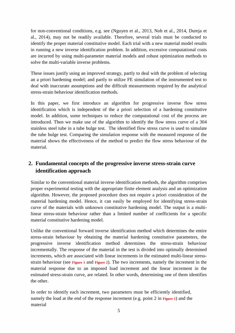
strain behaviour (see Figure 1 and Figure 2). The two increments, namely the increment in the

material response due to an imposed load increment and the linear increment in the

estimated stress-strain curve, are related. In other words, determining one of them identifies

the other.

In order to identify each increment, two parameters must be efficiently identified,

namely the load at the end of the response increment (e.g. point 2 in Figure 1) and the

material

6

hardening rate of the corresponding stress-strain increment, i.e. the slope of line

1’-2’ (in Figure 2).

The algorithm commences with the identification of the hardening behaviour by estimating

the initial yield point.. Then a multi-objective optimization algorithm determines the optimal

first hardening rate, slope of the line 1’-2’, and the first load increment, point 2. The next

yield point is determined as the maximum obtained simulated stress for the selected

increment, point 2’. Fixing the yield point at the maximum achieved stress has the benefit

that size and the slope of the next increment does not influence the estimated error of the last

identified increment. The algorithm continues this incremental procedure to identify the

multi-linear hardening model for the finite element simulation of the test which estimates

the response of the material.

Figure 1. Typical response of the material, and the estimated simulation response.

Figure 2. Actual and the estimated stress-strain curve.

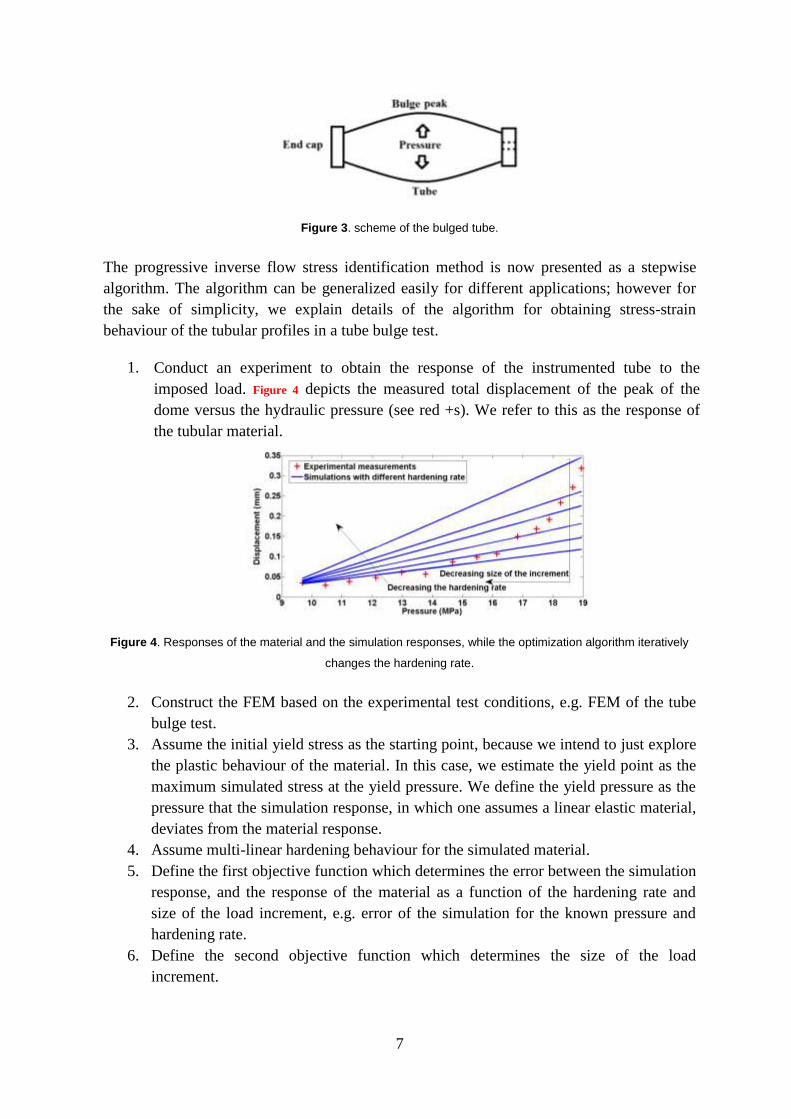
In this work, we select the total displacement of the tube’s bulge peak vs. internal

hydraulic pressure, see Figure 3, as the response of the material being tested. (Zribi et al.,

2013) and (Xu et al., 2008) already showed that the pressure-bulge height data contains

enough information for constructing an inverse problem to identify hardening parameters

of the material in a tube bulge test. Another objective function could be defined using,

strain or displacement of more points on the bulge surface. However, we preferred to use

the displacements of the other points on the surface for validating the results.

7

Figure 3. scheme of the bulged tube.

The progressive inverse flow stress identification method is now presented as a stepwise

algorithm. The algorithm can be generalized easily for different applications; however for

the sake of simplicity, we explain details of the algorithm for obtaining stress-strain

behaviour of the tubular profiles in a tube bulge test.

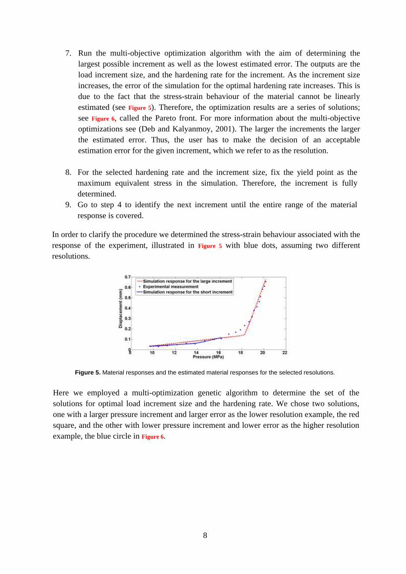
1. Conduct an experiment to obtain the response of the instrumented tube to the imposed load. Figure 4 depicts the measured total displacement of the peak of the

dome versus the hydraulic pressure (see red +s). We refer to this as the response of

the tubular material.

Figure 4. Responses of the material and the simulation responses, while the optimization algorithm iteratively

changes the hardening rate.

2. Construct the FEM based on the experimental test conditions, e.g. FEM of the tube

bulge test.

3. Assume the initial yield stress as the starting point, because we intend to just explore

the plastic behaviour of the material. In this case, we estimate the yield point as the

maximum simulated stress at the yield pressure. We define the yield pressure as the

pressure that the simulation response, in which one assumes a linear elastic material,

deviates from the material response.

4. Assume multi-linear hardening behaviour for the simulated material.

5. Define the first objective function which determines the error between the simulation

response, and the response of the material as a function of the hardening rate and

size of the load increment, e.g. error of the simulation for the known pressure and

hardening rate.

6. Define the second objective function which determines the size of the load

increment.

8

7. Run the multi-objective optimization algorithm with the aim of determining the largest possible increment as well as the lowest estimated error. The outputs are the load increment size, and the hardening rate for the increment. As the increment size increases, the error of the simulation for the optimal hardening rate increases. This is due to the fact that the stress-strain behaviour of the material cannot be linearly estimated (see Figure 5). Therefore, the optimization results are a series of solutions;

see Figure 6, called the Pareto front. For more information about the multi-objective

optimizations see (Deb and Kalyanmoy, 2001). The larger the increments the larger

the estimated error. Thus, the user has to make the decision of an acceptable

estimation error for the given increment, which we refer to as the resolution.

8. For the selected hardening rate and the increment size, fix the yield point as the

maximum equivalent stress in the simulation. Therefore, the increment is fully

determined.

9. Go to step 4 to identify the next increment until the entire range of the material

response is covered.

In order to clarify the procedure we determined the stress-strain behaviour associated with the

response of the experiment, illustrated in Figure 5 with blue dots, assuming two different

resolutions.

Figure 5. Material responses and the estimated material responses for the selected resolutions.

Here we employed a multi-optimization genetic algorithm to determine the set of the

solutions for optimal load increment size and the hardening rate. We chose two solutions,

one with a larger pressure increment and larger error as the lower resolution example, the red

square, and the other with lower pressure increment and lower error as the higher resolution

example, the blue circle in Figure 6.

9

Figure 6. Solutions of the multi-objective optimization.

We solved the algorithm for the first two increments. The resultant linearly estimated

stress-strain behaviours are illustrated in Figure 7, and the simulation responses using the

obtained stress-strain behaviour are superimposed on the experimental results already

depicted in Figure 5.

Figure 7. Estimated stress-strain behaviour for the selected resolutions.

Comparing the examples with higher and lower resolution shows how increasing the

resolution and size of the increments represent a trade-off. The former increases the

prediction accuracy, while the latter decreases the computational cost by estimating the

material hardening behaviour with fewer linear increments.

In order to apply the progressive inverse identification algorithm for identifying material

properties of the tubular material in the tube bulge test, the following observations are

noteworthy:

This method is used for characterizing the property of interest that is evolving with

load, e.g. hardening behaviour. When considering other properties as well (such as

friction and anisotropy) the relevant parameters describing these properties must be

determined separately (e.g. see (Zribi et al., 2013)). Alternatively an inverse

identification method which explores effects of the all parameters at the same time

must be employed. However, the latter needs a priori assumption of the constitutive

hardening model (e.g. see (Aguir et al., 2011, Prates et al., 2014, Bolzon and Talassi,

2013, Prates et al., 2015, Zhang et al., 2014)).

10

In the conventional forward inverse identification method, the suggested parameter

sets for every iteration of the optimization algorithm must be simulated considering

full load obtained by the experiment, e.g. point 4 in Figure 1. However, the stepwise

nature of the progressive inverse identification method allows simulating each

iteration with the pressure, lower than or equal to the maximum obtained load. This

results in a lower computational cost.

If the nature of the measurement error changes during the measurement, it is not

always possible to set an efficient fixed allowable error for linearly estimating all of

the increments. However, the obtained set of possible solutions always indicates the

minimum achievable error in contrast with the size of the increment. Note that it is

always advisable to select the measurement instrument based on the range of the

parameters of the interest, e.g. using a low range pressure gauge for beginning of the

tube bulge test and high range pressure gauge for the rest of the pressure

measurement. Therefore, the measurement noise is more consistent through the

entire range of the measurement.

If the selected increments are too short, the method models the noise rather than the

variation of the material properties.

In order to apply the method to obtain the material hardening behaviour after

instability, e.g. after occurrence of necking in uniaxial tensile test, we suggest using

imposed displacement as the load and measured reaction force as the response of the

material.

The aim of the next section of the paper is to demonstrate the application of the method to

obtain the stress-strain curve of a 304 stainless steel tube by conducting the tube bulge test

and applying the progressive inverse identification method to identify stress-strain

behaviour of the tube.

3. Stress-strain identification procedure for a 304 stainless steel tube

3.1 The tube bulge test

3.1.1 The experimental setup

In order to conduct the tube bulge test, a 63.5 mm × 1.4 mm laser-welded 304 stainless steel

tube was selected. One application of the selected tube is hydroforming of exhaust

manifolds in the automotive industry. Caps were welded to the ends of the sample tube. The

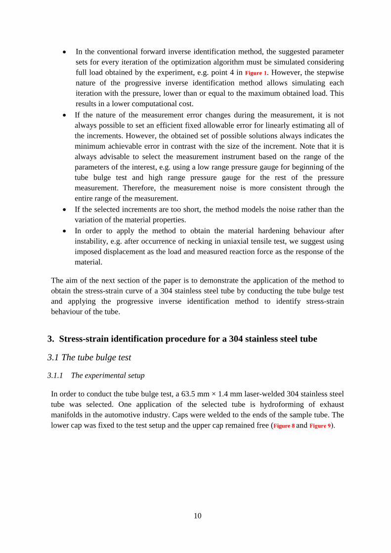
lower cap was fixed to the test setup and the upper cap remained free (Figure 8 and Figure 9).

11

Figure 8. Schematic of test sample

Initially a tube bulge forming die and a hand pump were employed to define the boundary

conditions of the test and to provide the pressure. However, high measurement noise caused

by the friction between the tube and the die, and also the pressure fluctuations, necessitated

a change in the setup.

Subsequently a single-stroke booster pump was devised to reduce the pressure fluctuations.

The pump comprised a single-stroke cylinder squeezed between the rams of a servo-

hydraulic universal testing machine. Since there is accurate velocity control on the actuator

speed, the bulge test could be conducted at a constant flow rate. By eliminating the

reciprocating motion inherent in the majority of positive-displacement hydraulic pumps,

the pressure noise could be reduced considerably (Figure 9).

A constant feeding rate of 233 ml/min for the bulge forming was selected. The measurement

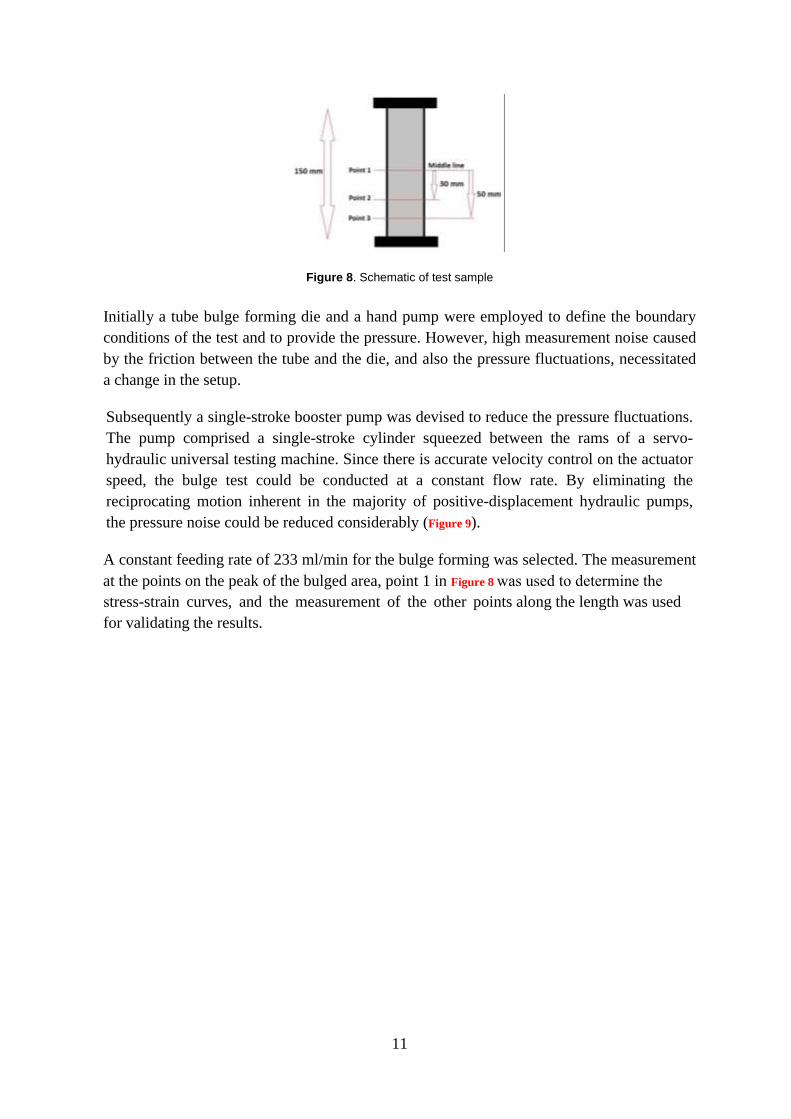
at the points on the peak of the bulged area, point 1 in Figure 8 was used to determine thestress-strain curves, and the measurement of the other points along the length was used

for validating the results.

12

Figure 9. The experimental setup.

3.1.2 Measurement methods

Because of the movement of the measuring points, a non-contact optical 3D measuring

system was employed. In order to measure displacement at the selected points, two high-

speed cameras were used to record the movement of the selected points on the surface of the

bulged area (see Figure 9 and Figure 10) with a frame rate of 3 frames per second (the high-

speed capability of the camera was not used in the current study). At the end of the test, the

results were exported to the GOM PONTOS software (2009) to calculate the displacement

of the points. The PONTOS software was used to detect the positions of the marked circles

on the surface of the tube.

An analogue pressure transducer (0-60 MPa) was coupled with the GOM to record the

applied pressure at the sampling times.

13

Figure 10. Test sample.

3.2 FEA of the tube bulge test

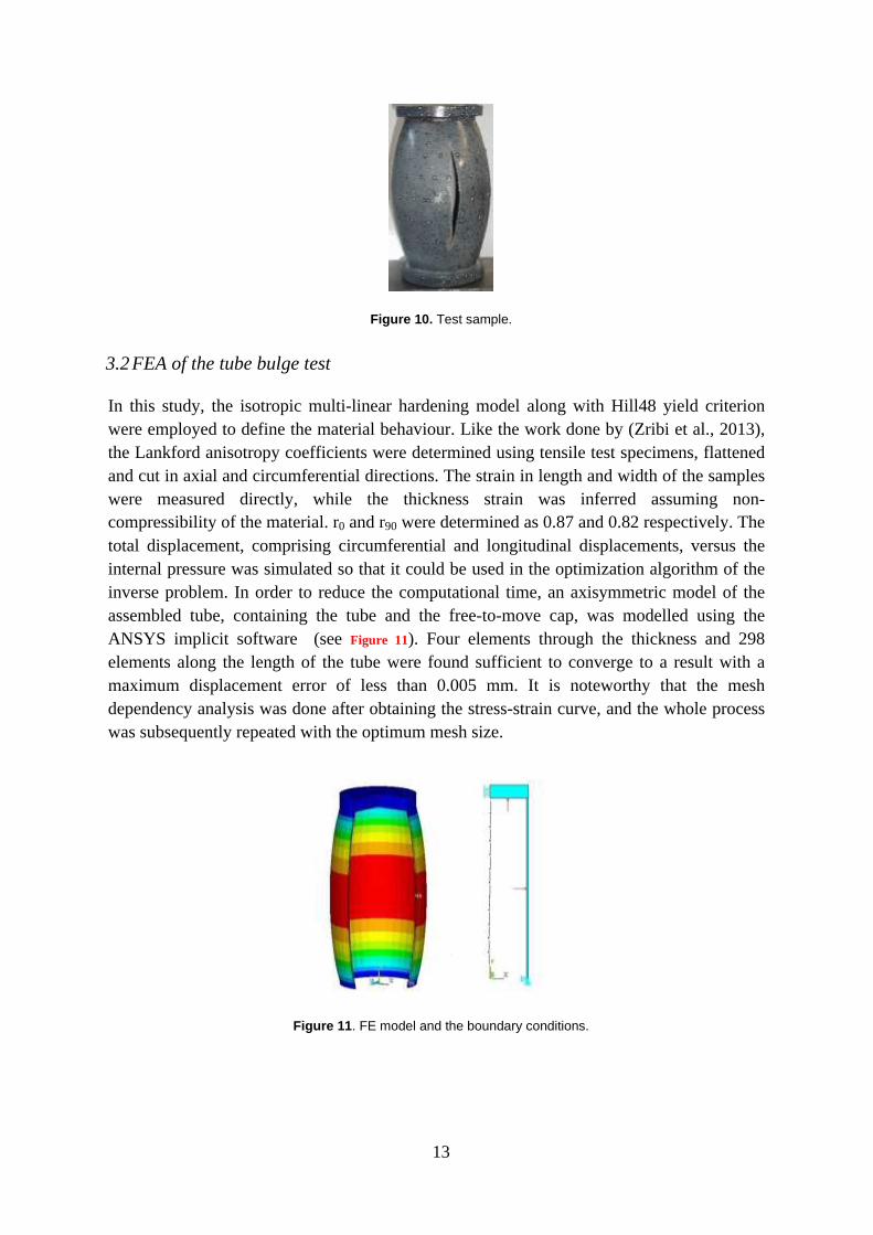
In this study, the isotropic multi-linear hardening model along with Hill48 yield criterion

were employed to define the material behaviour. Like the work done by (Zribi et al., 2013),

the Lankford anisotropy coefficients were determined using tensile test specimens, flattened

and cut in axial and circumferential directions. The strain in length and width of the samples

were measured directly, while the thickness strain was inferred assuming non-

compressibility of the material. r0 and r90 were determined as 0.87 and 0.82 respectively. The

total displacement, comprising circumferential and longitudinal displacements, versus the

internal pressure was simulated so that it could be used in the optimization algorithm of the

inverse problem. In order to reduce the computational time, an axisymmetric model of the

assembled tube, containing the tube and the free-to-move cap, was modelled using the

ANSYS implicit software (see Figure 11). Four elements through the thickness and 298

elements along the length of the tube were found sufficient to converge to a result with a

maximum displacement error of less than 0.005 mm. It is noteworthy that the mesh

dependency analysis was done after obtaining the stress-strain curve, and the whole process

was subsequently repeated with the optimum mesh size.

Figure 11. FE model and the boundary conditions.

14

3.3 Surrogate modelling

A genetic multi-objective optimization algorithm (implemented as ‘’gamultiobj’’ in Matlab

(2015) using the default parameters), was adopted to solve the multi-objective optimization

problem. The algorithm calls for multiple evaluations of the objective functions. Running a

finite element simulation to evaluate the objective functions for each call, drastically

increases the computational cost of the entire of the algorithm. To deal with this, we

employed a cheap-to-evaluate surrogate model of the FEM. In other words, the algorithm

calls the surrogate model for the objective function evaluation rather than calling the FEM.

The surrogate model used in this study is an Artificial Neural Network which was trained to

replace the computationally expensive FEM. Here the term training refers to identifying

parameters of the regression model (weights of the basis function used in the ANN). In order

to train the ANN, it is common practice to construct the set of the material parameters, and

the corresponding finite element simulation responses, and then the ANN is trained to

estimate the FEM response for the unseen parameter. e.g. see (Aguir et al., 2011). This set is

known as the training set.

In order to identify each increment, the ANNs are trained. We simulated the experiment

using six different hardening rates covering high and low hardening rates for each increment,

assuming an initial large increment size, e.g. see Figure 1. It is better to adjust the simulation

pressure high enough to ensure that the optimization algorithm can search for possible large

increments. However for the initial increments we set the simulation pressure lower than the

maximum obtained pressure in the experiment to reduce the computational costs. Selecting

these lower pressures for the simulations does not degrade the accuracy, but the

computational cost increases by imposing small increments to the algorithm, while it is not

necessary. The hardening rates were used as inputs in the training set.

We did not directly introduce the high dimensional displacement vectors from the simulated

responses as the outputs of the training set. Instead, the first principal component (PC) of the

simulation response vectors served as the output of the training set to construct the surrogate

model. We replaced the original simulation response vectors with the PCs to simplify the

ANN architecture. PCs were obtained by projecting the response vectors into the space of the

principal directions of the training set. For more information about principal component

analysis see (Jolliffe, 2002). This projection technique allows reducing the dimensionality of

the vectors, while most of the variance in the data is retained. For instance, using the first

principal component for the simulation responses shown in Figure 4 reduced the response

dimensions from 15 to 1, while it retained more than 99% of the variance. Hence, the authors

strongly suggest using PCs as substitute for the original vectors in constructing the surrogate

model to simplify the structure while maintaining the accuracy.

The constructed training set is then used to train the ANNs. This very simple network

contains one neuron for the input layer, two neurons N1 and N2 (see Figure 12) for the hidden

layer, and one neuron for the output layer. The selected training algorithm is the Bayesian

‘’trainbr’’ training function in Matlab. Figure 12 schematically illustrates

15

the procedure of constructing the cheap-to-evaluate surrogate model of the finite element

simulation.

Figure 12. Schematic of constructing the surrogate model.

Figure 13 illustrates the entire of the proposed computationally efficient inverse method, used

to estimate stress-strain behaviour of the tube, subjected to tube bulge test.

16

Figure 13. The efficient inverse identification procedure used to identify the stress-strain behaviour

of the tube in the tube bulge test.

17

4. Results and discussion

In order to provide a baseline for evaluating the efficacy of the newly proposed method, a

comparative study was done using the conventional forward inverse identification method.

This method assumes an a priori hardening model, to capture the stress-strain behaviour of

the tube. By way of example, the procedure used in (Zribi et al., 2013) was applied to

identify parameters of the Ludwik model for the response of the material obtained from the

bulge test. The FEA of the test was employed to simulate the response of the experiment.

In these calculations the simulation pressure was limited to 25.5 MPa, although the

maximum pressure obtained in the test was 26.4 MPa. The characterisation process was

therefore restricted to a part of the stress-strain curve associated with the tube bulge test

response. This was because the FEA of the material parameters suggested by the

optimization algorithm could not be made to converge for many of the material parameters

suggested by the optimization algorithm, due to the instability of the numerical model given

the material characteristic at the selected pressure. This is more severe when the suggested

stress-strain response approaches the stress-strain behaviour of the material. Non-

convergence of the FEA for the suggested parameters can therefore degrade the efficiency

of the optimization algorithm.

The best fitted Ludwik model is represented by

(1)

where σ and ε denote stress and plastic strain. Using this Ludwik model to simulate the

process, a simulated response may be found which is plotted on the measured material

response in Figure 14.

Figure 14. Simulation response of the identified Ludwik model and the measured material response.

The Ludwik material model is clearly not able to accurately predict the material response for

the selected part of the experiment. Other material hardening models could also be tried, and

the optimization algorithm could be restarted at different initial points to result in possibly a

more accurate stress-strain curve. This example was the first attempt of the authors to obtain

the stress-strain behaviour of the selected tube. However, the inaccurate result, and high

computational expense of each trial, restarting the optimization algorithm and selecting

18

different hardening models, motivated us to opt for a new inverse identification approach as

an alternative to the conventional inverse problem. We here employ the progressive inverse

stress-strain identification approach to estimate the material hardening behaviour.

In order to estimate the stress-strain characteristic of the tube, we limited the acceptable

estimation error for determining parameters of the first three increments to 4×10-4

mm2. This

error is the average of the squared differences of the measured displacements and the

simulated displacements of the measured points within each increment. In addition, the

acceptable estimation error for the rest of the increments is limited to 2×10-2

(dimensionless)

as the average of the squared relative error of the simulated and measured displacement

within each increment, as it is used in (Zribi et al., 2013, Aguir et al., 2011). We used

absolute error for the first three increments because the magnitude of some measurements in

the beginning of the response measurement is very small while their measurement noise is

of the same order as the values. Therefore, dividing the differences by a very small number

for calculating the relative error imposes a dominant error for calculating the average error

within the increment. This problem is mostly due to the fact that we use the same devices

for measuring very low and very high magnitudes during the test. The objective of this

paper is however not to study different types of error and variations of the error along the

experiment. More research could be conducted to assess the effects of the different objective

functions.

Applying the progressive inverse material identification method to the response of the bulge

test, the stress-strain behaviour of the material is identified. As it is illustrated in Figure 15 the

algorithm estimates the hardening behaviour with 7 linear increments.

Figure 15. Identified multilinear stress-strain curve against the best fitted Ludwik model.

In order to evaluate the accuracy of the stress-strain behaviour obtained, the identified

curve is used to simulate the experiment. Responses of the simulation and responses of the

experiment are compared in Figure 16. Measurements at point 1 (see Figure 8) were employedin the progressive inverse identification method. The responses of the tube at points 2 and 3

were not used in the calculations. They could therefore be used to validate the result.

Clearly, using the obtained stress-strain behaviour in the simulation process allows the

simulations to accurately follow the material responses at the selected points.

19

Figure 16. Response of the tube bulge simulation using the obtained material behaviour.

5. Conclusion

This study proposed an inverse identification approach to identify the flow stress of the

materials. The proposed approach estimates the stress-strain behaviour with a multi-linear

curve with adjustable resolution. In addition, a procedure to reduce the total computational

cost was explained. The proposed method retains the benefits of the both analytical and

conventional inverse flow stress identification approaches. On the one hand the method is

independent of selecting an a priori constitutive hardening model, and on the other hand

various simplifying assumptions and difficult measurements are avoided.

The presented method was employed to identify stress-strain behaviour of a 304 stainless

steel tube in a tube bulge test. The comparison between response of the simulation, using the

obtained material behaviour, and the response of the material showed the efficiency of the

method.

As a result, the progressive inverse identification method can be employed efficiently to

identify the stress-strain behaviour of the materials with an unknown hardening constitutive

model subjected to complicated stress states, within a reasonable time. This is possible

owing to the changes proposed to the conventional inverse forward identification method.

References

ANSYS® Academic Research,Release 14,5.

2009. GOM Optical Measuring Techniques. PONTOS User Manual – Software. PONTOS. 6.2 ed.

20

2015. Matlab. R2015 ed. Natick, Massachusetts: The Mathworks Inc.

AGUIR, H., BELHADJSALAH, H. & HAMBLI, R. (2011), ''Parameter identification of an elasto-

plastic behaviour using artificial neural networks-genetic algorithm method'', Materials and

Design, 32, 48-53.

BOCCIARELLI, M., BULJAK, V., MOY, C. K. S., RINGER, S. P. & RANZI, G. (2014), ''An

inverse analysis approach based on a POD direct model for the mechanical characterization of

metallic materials'', Computational Materials Science, 95, 302-308.

BOLZON, G. & TALASSI, M. (2013), ''An effective inverse analysis tool for parameter identification

of anisotropic material models'', International Journal of Mechanical Sciences, 77, 130-144.

BORTOT, P., CERETTI, E. & GIARDINI, C. (2008), ''The determination of flow stress of tubular

material for hydroforming applications'', Journal of Materials Processing Technology, 203,

381-388.

COONEY, G. M., MOERMAN, K. M., TAKAZA, M., WINTER, D. C. & SIMMS, C. K. (2015),

''Uniaxial and biaxial mechanical properties of porcine linea alba'', Journal of the Mechanical

Behavior of Biomedical Materials, 41, 68-82.

DEB, K. & KALYANMOY, D. (2001). Multi-Objective Optimization Using Evolutionary

Algorithms, John Wiley & Sons, Inc.

DUREJA, A. K., SINHA, S. K., PAWASKAR, D. N., SESHU, P., CHAKRAVARTTY, J. K. &

SINHA, R. K. (2014), ''Modelling flow and work hardening behaviour of cold worked r–

2. b pressure tube material in the temperature range of 3 – , Nuclear Engineering

and Design, 269, 52-56.

GERMAIN, G., MOREL, A. & BRAHAM-BOUCHNAK, T. (2013), ''Identification of material

constitutive laws representative of machining conditions for two titanium alloys: Ti6Al4V

and Ti555-3'', Journal of Engineering Materials and Technology, Transactions of the ASME,

135.

HWANG, Y. M., LIN, Y. K. & ALTAN, T. (2007), ''Evaluation of tubular materials by a hydraulic

bulge test'', International Journal of Machine Tools and Manufacture, 47, 343-351.

HWANG, Y. M. & WANG, C. W. (2009), ''Flow stress evaluation of zinc copper and carbon steel

tubes by hydraulic bulge tests considering their anisotropy'', Journal of Materials Processing

Technology, 209, 4423-4428.

JOLLIFFE, I. T. (2002). Principal component analysis, Springer-Verlag.

KANG, S.-H., LEE, Y.-S. & LEE, H. W. (2014), ''Evaluation of flow stress and damage index at large

plastic strain by simulating tensile test of Al6061 plates with various grain sizes'',

International Journal of Mechanical Sciences, 80, 54-61.

KOÇ, M., AUE-U-LAN, Y. & ALTAN, T. (2001), ''On the characteristics of tubular materials for

hydroforming - experimentation and analysis'', International Journal of Machine Tools and

Manufacture, 41, 761-772.

LI, G., XU, F., SUN, G. & LI, Q. (2014), ''Identification of mechanical properties of the weld line by

combining 3D digital image correlation with inverse modeling procedure'', International

Journal of Advanced Manufacturing Technology, 74, 893-905.

21

LIANFA, Y. & CHENG, G. (2008), ''Determination of stress-strain relationship of tubular material

with hydraulic bulge test'', Thin-Walled Structures, 46, 147-154.

LUCZYNSKI, K. W., STEIGER-THIRSFELD, A., BERNARDI, J., EBERHARDSTEINER, J. &

HELLMICH, C. (2015), ''Extracellular bone matrix exhibits hardening elastoplasticity and

more than double cortical strength: Evidence from homogeneous compression of non-tapered

single micron-sized pillars welded to a rigid substrate'', Journal of the Mechanical Behavior

of Biomedical Materials, 52, 51-62.

NEMAT-ALLA, M. (2003), ''Reproducing hoop stress-strain behavior for tubular material using

lateral compression test'', International Journal of Mechanical Sciences, 45, 605-621.

NGUYEN, N. T., LEE, M. G., KIM, J. H. & KIM, H. Y. (2013), ''A practical constitutive model for

AZ31B Mg alloy sheets with unusual stress-strain response'', Finite Elements in Analysis and

Design, 76, 39-49.

NOH, W., KOH, Y., SEOK, D.-Y., WAGONER, R. H., BARLAT, F. & CHUNG, K. (2014),

''Mechanical property of magnesium alloy sheet with hardening deterioration at warm

temperatures and its application for failure analysis: Part I - property characterization'',

International Journal of Material Forming, 1-9.

PRATES, P. A., OLIVEIRA, M. C. & FERNANDES, J. V. (2014), ''A new strategy for the

simultaneous identification of constitutive laws parameters of metal sheets using a single

test'', Computational Materials Science, 85, 102-120.

PRATES, P. A., OLIVEIRA, M. C. & FERNANDES, J. V. (2015), ''Identification of material

parameters for thin sheets from single biaxial tensile test using a sequential inverse

identification strategy'', International Journal of Material Forming, 1-25.

SABOORI, M., CHAMPLIAUD, H., GHOLIPOUR, J., GAKWAYA, A., SAVOIE, J. &

WANJARA, P. (2014), ''Evaluating the flow stress of aerospace alloys for tube hydroforming

process by free expansion testing'', International Journal of Advanced Manufacturing

Technology, 72, 1275-1286.

STRANO, M. & ALTAN, T. (2004), ''An inverse energy approach to determine the flow stress of

tubular materials for hydroforming applications'', Journal of Materials Processing

Technology, 146, 92-96.

SUN, G., XU, F., LI, G., HUANG, X. & LI, Q. (2014), ''Determination of mechanical properties of

the weld line by combining micro-indentation with inverse modeling'', Computational

Materials Science, 85, 347-362.

XU, Y., CHAN, L. C., TSIEN, Y. C., GAO, L. & ZHENG, P. F. (2008), ''Prediction of work-

hardening coefficient and exponential by adaptive inverse finite element method for tubular

material'', Journal of Materials Processing Technology, 201, 413-418.

ZHANG, S., LEOTOING, L., GUINES, D., THUILLIER, S. & ZANG, S.-L. (2014), ''Calibration of

anisotropic yield criterion with conventional tests or biaxial test'', International Journal of

Mechanical Sciences, 85, 142-151.

ZRIBI, T., KHALFALLAH, A. & BELHADJSALAH, H. (2013), ''Experimental characterization and

inverse constitutive parameters identification of tubular materials for tube hydroforming

process'', Materials & Design, 49, 866-877.