Flow rate evaluation in parallel pump arrangements: Two case … · · 2017-04-18Flow rate evaluation in parallel pump arrangements: Two case studies J. Lanzersdorfer y M. Schmidt

Flow rate evaluation in parallel pump

arrangements: Two case studies

J. Lanzersdorfer∗† M. Schmidt∗ J. Pichler∗

July 28, 2016

Abstract

Hydraulic tests on pumps for industrial applications pose several

challenges for measurement engineers. Among them, conditions for

pressure and �ow rate measurement do usually not comply with stan-

dards for precision measurements. It is therefore common to perform

factory acceptance tests to achieve high accuracy. In certain cases per-

formance testing on site remains inevitable. In here, we present two

case studies of o�-factory measurements using index testing on parallel

arranged pumps. The focus of these studies is on the �ow rate deter-

mination which comprises the choice and application of an adequate

measurement method, a �ow rate calibration strategy and a reliability

test of the results. It is �nally possible to determine the weights of

the measured branch �ow rates. Comparisons with accessible perfor-

mance data correlate very well and makes this kind of proceeding a

powerful tool for volumetric discharge determination at unfavorable

�ow conditions.

∗Andritz AG, Stattegger Strasse 18, 8045 Graz - Austria†Corresponding author: [email protected]

1

11th IGHEM Conference, Linz/Austria, August 24�26, 2016 2

1 Introduction

The industry typically demands reliability of the production process and lowpower consumption from a pump, the e�ciency is a minor matter. However,knowledge of the �ow rate is of major interest for cooling water purposes.Cooling water circuits are mostly equipped with several parallel arrangedpumps to avoid production losses and to adapt the number of operatingpumps to the actual needs. The latter premises the knowledge of two subse-quent facts to optimize the production process:

• the total �ow rate and

• the �ow proportion provided by an individual pump.

Pump testing at industrial facilities [1] challenges us since the structuralrequirements for proper measurement conditions are often inconsistent with�nancial aspects of the production. We therefore need to analyze the hy-draulic, the metrological and the production related aspects of a test cam-paign in advance. As a result, we end up with a tailor-made �ow rate cali-

bration strategy, whose aim is to regress certain branch �ow rates to availableindex parameters. The procedure of this strategy usually antecedes or goesalong with the main measurements. In order to show the application of such�ow rate calibrations we present two case studies of real test campaigns inthe subsequent sections. In both cases single-path ultrasonic �owmeters inre�ection mode were used which usually frown upon the turbine test com-munity. However, the application of clamp-on acoustic �owmeters representsa cheap and � if you know how to use them � a reliable method for �owindication in the pump business.

The �rst case study gives insight into simultaneous measurements on �veparallel arranged pumps which feed a re�nery and neighboring industrialplants with cooling water. We present here the metrological and mathemat-ical steps to determine the individual branch �ow rates under � what testcodes usually denote as � unfavorable measurement conditions.

The second study shows how the total �ow rate in a cooling water sys-tem of a thermal power plant was determined by calibrating the �ow ratemeasurements on three parallel system branches. Di�erent �ow functions

are investigated towards statistical �tness and physical plausibility. We usedthis information to check and optimize the operating points in single-pumpmode and dual-pump mode.


2 Case study: Determination of branch �ows of

�ve main cooling pumps without interrupt-

ing the production process

2.1 Description

In November 2015 we conducted a test campaign on the main cooling watercircuit of a re�nery, which is operated by OMV Deutschland GmbH, closeto the town of Burghausen/Germany. There the re�nery process plant andother neighboring industrial plants are continuously fed with cooling waterby up to �ve parallel-driven vertical line shaft pumps (VLSPs). The powerinput per pump unit is approximately 1 MW, their service life and their hy-draulic contour di�er. The main target of the campaign was to evaluate theindividual pump performance (i.e., Q-H-P ) without interrupting the produc-tion process. Here, we focus on the �ow rate evaluation of each pump branch.

Figure 1 shows a simpli�ed P&ID. The VLSPs suck in water from anopen basin and feed a collector pipe which provides cooling power to theindividual consumers. Downstream the consumers the heated water is trans-mitted to the cooling tower where the thermal energy dissipates into theforced circulating air. Finally, the water drops back into the suction basin.

v1 v2 v3 v4 v5 Qref

cooling

tower

consumers

Figure 1: Simpli�ed P&ID of the test setup on the main cooling water circuit at

Burghausen re�nery: Qref and vi denote permanently and temporarily installed

�ow measurements, respectively.


The hydraulic conduit downstream the high-pressure �ange of each VLSPis established by a horizontal part of 5D length, a 90◦ bend with 2D curva-ture radius, a vertical straight part with 10D length and another 90◦ bendleading to the horizontally aligned collector pipe. The initial, horizontal partcomprises a swing type check valve (CV) � except for the pipe branch ofpump #1 � followed by a manually operated butter�y valve (BV). There ex-ists no adequate tappings for pressure measurements downstream the pump�ange.

2.2 Test setup and procedure

Challenges and metrological strategy There is no general shutdown ofthe cooling circuit scheduled. The production lines need enough amount ofcooling water with a minimum of three cooling pumps running. The applica-tion of an accurate, absolute �ow measurement method on each pump branchwould require an intervention into the production process, which stands with-out question. The additional costs for installations and modi�cations alsomade it less attractive for the client.

A combination of collector pipe �ow measurement and secondary �owmeasurements on each branch as used for index tests [2] seemed to be bestin line with the targets and the requirements. If possible the use of propermeasurement of pressure losses along conduits represents a cheap and highlyreliable method for �ow indication. Unfortunately, there existed only fewtappings which were poorly positioned next to hydraulic obstacles. We con-sequently decided to indicate the branch �ow rates by means of the acoustictransit time method (ATTM) in single-path mode. We expected to ade-quately reduce the impact of the local cross �ow on the velocity measure-ments in axial direction by arranging the sensor pairs in re�ection mode. Butthe informative value of the measured velocity v remained questionable be-cause of the presence of an axially asymmetric �ow pattern. This was mainlycaused by the upstream 90◦ bend. However, the normalized �ow pattern atthe acoustic measurement section was considered to be independent underchanges of the branch �ow rate as long as the hydraulic contour downstreamthe pump's high-pressure �ange remained unchanged.1 The axial velocitymeasured along an arbitrarily oriented2 acoustic path is therefore alwaysproportional to the real �ow rate and a good estimate of the real branch �ow

1For instance, the �ow distribution is signi�cantly disturbed by changing the openingangle of the BV.

2We disregard the trivial cases of path angles parallel and perpendicular to the pipeaxis.


rate yieldsQi = ci · Aivi (1)

with the hydraulic cross section Ai and the unknown proportionality fac-tor ci. The total �ow Qref can be calculated by summing up the proportionsmeasured by the permanently installed devices (Venturi tube and ori�ce mea-surements).

Calibration strategy Since the water density at the measurement sectionsof the branch �ow rates and of the permanent �owmeters does not alter sig-ni�cantly, the continuity equation simpli�es to its volumetric representationand it yields

Qref∼=

5∑i=1

Qi (2)

or

Qref∼=

5∑i=1

ci · Aivi, (3)

respectively (view Figure 2). The right side of equation (3) represents amodel function � or simply called �ow function � whose unknown coe�cientshave to be determined by linear regressing the observations Qref to the in-dependent variables vi. At least six

3 di�erent operating points are required,where measurements of vi's and Qref have to be taken, to check the statisticalsigni�cance of the calculated coe�cients ci. There are three possibilities tochange the operating conditions, which also can be used simultaneously:

1. Changing the �ow resistance4 downstream collector pipe, for instance,by opening/closing one or more valves along the production lines.

2. Changing the �ow resistance of one or more pump branches by changingthe BV opening.

3. Changing the combination of pump units under operation.

We wanted to avoid possibility 1 because the complex pipe branching athand makes it almost impossible to eliminate any risk of failure indication

3The statistical degree of freedom need to be larger than zero:

df = n−m > 0

where n and m denote the number of observations and the number of regressors, respec-tively.

4More precisely: the dimensionless pressure loss coe�cient ζ.


Q1

Qref

Q2

Q3

Q4

Q5

Figure 2: Flow diagram

in the subsequent production lines. The second possibility would stronglyin�uence the �ow pattern at the acoustic measurement section and, thus,the determination of the axial �ow velocity v. The proportionality between�ow estimate and measured axial velocity could not be established anymore.Finally, changing the number and choice of running pumps units remainedthe only degree of freedom to adjust the operating conditions. With therequirements of three units running at minimum, we obtain the maximumnumber of di�erent operation points (= observations) by

nmax =5∑

k=3

(nk

)= 16 . (4)

That is, there are 1, 5 and 10 di�erent pump combinations under �ve-units,four-units and three-units operation, respectively. With in total

df = nmax −m = 11

degrees of freedom we �nally should end up with a low random uncertaintyof the calibration coe�cients ci if the model function in (3) described theobserved behavior well.


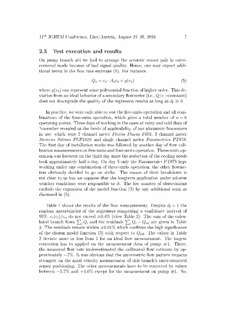
2.3 Test execution and results

On pump branch #4 we had to arrange the acoustic sensor pair in cater-cornered mode because of bad signal quality. Hence, one may expect addi-tional terms in the �ow rate estimate (1). For instance,

Q4 = c4 · A4v4 + g(v4) (5)

where g(v4) can represent some polynomial function of higher order. This de-viation from an ideal behavior of a secondary �owmeter (i.e., Q/v =constant)does not downgrade the quality of the regression results as long as df � 0.

In practice, we were only able to test the �ve-units operation and all com-binations of the four-units operation, which gives a total number of n = 6operating points. Three days of working in the open at rainy and cold days ofNovember revealed us the limits of applicability of our ultrasonic �owmetersin use, which were 2 channel meter Flexim Fluxus F601, 2 channel meterSiemens Sitrans FUP1010 and single channel meter Panametrics PT878.The �rst day of installation works was followed by another day of �ow cali-bration measurements on �ve-units and four-units operation. Three-units op-eration was foreseen on the third day since the reduction of the cooling needstook approximately half a day. On day 3 only the Panametrics PT878 keptworking under any combination of three-units operation, the other �owme-ters obviously decided to go on strike. The reason of their breakdown isnot clear to us but we suppose that the longterm application under adverseweather conditions were responsible to it. The low number of observationsexclude the expansion of the model function (3) by any additional term asdiscussed in (5).

Table 1 shows the results of the �ow measurements. Despite df = 1 therandom uncertainties of the regressors comprising a con�dence interval of95%, er(ci)/ci, do not exceed ±0.4% (view Table 2). The sum of the calcu-lated branch �ows

∑iQi and the residuals

∑iQi −Qref are given in Table

3. The residuals remain within ±0.01% which con�rms the high signi�canceof the chosen model function (3) with respect to Qref. The values in Table2 deviate more or less from 1 for an ideal �ow measurement. The largestcorrection has to applied on the measurement data of pump #4. There,the measured �ow rate underestimated the calibrated �ow estimate by ap-proximately −7%. It was obvious that the asymmetric �ow pattern impactsstrongest on the axial velocity measurement of this branch's cater-corneredsensor positioning. The other measurements have to be corrected by valuesbetween −5.7% and +4.0% except for the measurement on pump #1. So,


there is no clear tendency in adjusting the values in positive or in negativedirection. We installed the re�ection mode arranged sensor pairs similarilyin azimuthal and in longitudinal locations but we have used di�erent types ofsensors and �owmeters. Therefore, it is not possible to apportion the metro-logical quality among the test setup or the hydraulic �ow behavior.

Let us take a closer look onto the results of pump #1. Taking account ofthe random uncertainty the �ow measurement on this unit can be consideredas ideal measurement. We actually had better metrological conditions onthis unit compared to the setup on the other four units. The �ange tran-sitions are smooth at this unit, which made the head measurements morereliable. Pump #1 is smaller in geometry and the branch pipe has no CV.The nominal pipe lengths are longer which favors the in�ow conditions intothe acoustic measurement zone. Despite its age of more than 25 years nocavitation related abrasion damages were detected so far on the hydrauliccontour [3]. This gives us the opportunity to compare our �ow measure-ments with the factory acceptance test on this unit from 1990. Figure 3clearly shows that the acceptance test curve could be reproduced well sincethe largest absolute deviation in head is only 0.5%.

We conclude that the calibration procedure of each branch �ow velocitymeasurement vi with respect to reference �ow rate Qref was successful. Aproof of the correctness of the reference �ow rate by comparing it with anabsolute �ow measurement method is missing. However, the veri�cation ofthe pump characteristics of pump #1 gives an indication for the validityof the reference �ow. Within the �ow rate interval Qi ∈ [0.6, 0.8] ·Qrated theproportionality between axial velocity as measured and branch �ow rate couldbe ver�ed with high signi�cance. But outside this interval, the metrologicalbehavior may di�er and cannot be described by equation (1) anymore.


Table 1: Normalized measurement results

# A1v1Qrated

A2v2Qrated

A3v3Qrated

A4v4Qrated

A5v5Qrated

Qref

Qrated

- - - - - - -

1 0.00009 0.91725 0.97508 0.93403 0.99999 3.847162 0.59551 0.79763 0.89294 0.83381 0.89647 4.034053 0.79319 0.00022 1.00248 0.95711 1.03134 3.768914 0.79986 0.93167 0.00011 0.94415 1.03239 3.753895 0.80366 0.93415 1.01346 0.00149 1.04005 3.747876 0.79981 0.92718 0.99244 0.95106 0.00033 3.75090

Table 2: Results of the regression analysis (df = 1, con�dence interval 95%)

parameter unit value ± random uncertainty

c1 - 1.002± 0.004c2 - 1.040± 0.003c3 - 0.975± 0.003c4 - 1.069± 0.003c5 - 0.943± 0.003

Table 3: Comparison of reference and regression �ow rate

# Qref

Qrated

∑i Qi

Qrated

residual

- - - -

1 3.84716 3.84709 -0.000072 4.03405 4.03428 0.000233 3.76891 3.76887 -0.000054 3.75389 3.75386 -0.000045 3.74787 3.74782 -0.000046 3.75090 3.75086 -0.00004


Figure 3: Pump #1: Comparison of the branch-�ow-calibrated performance test

(circle) with the original factory acceptance test data from 1990 (line). Measure-

ment data are speed-converted.


3 Case study: Optimization of pump operation

points on main cooling circuit

3.1 Description

In April 2016 the Knippegroen gas power plant, which is located close toGhent/Belgium, was subject of general revision works. During the down timeof the power generation unit the operating points of the two main coolingpumps should be checked and � if necessary � it should be optimized forsingle-pump mode and for dual-pump mode. Referring to the P&ID in Figure4 cooling water is stored below the cooling tower in an open basin. Twoparallel arranged VLSPs pump the water into the subterranean, cold collectorpipe leading to the power house. There, the collector pipe subdivides into twomajor pipes, which feed the condenser to cool the water of the primary circuit,and a minor pipe providing cooling power to auxiliary devices. All threebranches unite subsequently in the hot collector pipe situated underground.It leads back to the cooling tower, where the water temperature is reduced byforced air-conditioning. The pumps require approximately 1 MW of electricalpower each. Both have identical hydraulic contours.

coolingtower

condenser

coolingtasks

v1

v2

v3

dp1

dp2

Figure 4: Simpli�ed P&ID of the test setup on the main cooling water circuit at

Knippegroen gas power plant: vi denote the temporarily installed �ow velocity

measurements, ∆pi are the permanently installed pressure devices.


3.2 Test setup and procedure

Challenges and metrological strategy The pipings of the cooling cir-cuit is made of glass-�ber reinforced plastic (GRP) except those parts usedfor direct heat-exchange. The automatic-operated BV downstream the high-pressure pump �ange is not designed for throttle purposes but only for start-ing and stopping the pump. There is no possibility in installing an acousticclamp-on �owmeter onto the pump branch anywhere between high-pressure�ange and the conjunction with the subterranean collector pipe. The acces-sible pipeworks outside and inside the powerhouse is very complex. A fewpressure tappings are available, but their positionings and the asymmetric�ow pattern give rise to distrust of the measurement quality. The two BVsdownstream the condenser are fully opened at dual-pump mode and partlyopened at single-pump mode. The cooling branch for auxiliary tasks is neverthrottled under normal plant operation.

There exists permanent measurement devices for the pressure losses ofeach condenser branch, ∆p1 and ∆p2, which can be used to indicate the�ow rate Q1 and Q2, respectively. The quality of theses measurements wasunknown beforehand. Therefore, we decided to record these pressures forbackup reasons but ATTM should be used as primary �ow indication. Wechose measurement sections upstream the condenser or any cooling task forthe axial �ow velocity measurements. On each branch pipe an ultrasonic sen-sor pair was mounted in re�ection mode. Here again, we made a simpli�edassumption that the normalized �ow pattern at the measurement sectionsremain independent from the �ow rate. And we avoid any unpredictableimpact onto the velocity distribution by �ow throttling at the manually op-

Q1

Q2

Q3

Qref

QA

QB

Figure 5: Flow diagram


erated BVs far downstream. Figure 5 shows a simpli�ed representation ofthe cooling water �ow. The down time of the power generating unit o�eredadditional possibilities in operating the cooling circuit. The auxiliary branchand at maximum one of the major branches could have been put out of ser-vice if desired. Anyhow, we did not want to perform any tests on operatingconditions for which the cooling water circuit maybe has not been designed.The calibration tests were partly done with a closed auxiliary pipe.

Calibration strategy Since it is impossible to measure any reference �owrate in the underground collector pipe we cannot proceed with the branch�ow calibration as described in the previous case study. We need to subdivideour calibration routine into three steps:

1. We keep one pump unit running under stable conditions and maintaina constant static pump head Hst by adjusting the openings of the BVsdownstream the acoustic measurement sections. Neglecting any exces-sive change of the �uid viscosity the stable pressure head guaranteesa constant volumetric �ow rate. We set this unknown total �ow rateQref = Qrated because � at this state � there is no need for the correctvalue. The continuity law under constant density yields

fi ∼= Qref = Qrated (6)

with the model functions of the �ow fi, which are introduced subse-quently.As described in the previous subsection there are several possibilitiesin indicating the branch �ow rates by clamp-on �owmeters and bymeasurements of pressure losses. Primarily, we use the acoustic mea-surements on all three branches, yielding the model function

f1 =3∑

i=1

c1i · Aivi. (7)

We assume discharge-independent, normalized velocity pro�les at allmeasurement sections with cross-section Ai. Together with the sensorarrangements in re�ection mode the simple representation of (7) is rea-sonable. Using the pressure loss parameters ∆p1 and ∆p2 and assuming(Qi)

2-dependency, we alternatively may de�ne

f2 =2∑

i=1

c2i ·(

∆pi1 bar

)0.5

+ c23 · A3v3. (8)


Finally, a more general representation of (8)

f3 =2∑

i=1

c3i ·(

∆pi1 bar

)ni

+ c33 · A3v3, (9)

is investigated in addition to (7) and (8). These three de�nitions aremost probable and physically relevant. Other �ow functions are notdiscussed in this paper.The number of regressors m equals 3 and 5 for the model functions(7)�(8) and 9, respectively. We hence need at least n = 6 calibrationmeasurements to evaluate all model functions statistically.

2. Here, the missing proportionality factor between the scaled model test�ow and the calibrated �ow has to determined. Additionally, a plausi-bility check of the model function is done within the normal operatingrange in single-pump mode. For this, an index test on a single pumpunit is executed. Comparing the measured pump characteristics withscaled model test data under assimilable NPSH values yields the pro-portionality coe�cient

ki =Qmodel

fi. (10)

Depending on the choice of the model function we obtain the total �owrate by

Q = ki · fi =3∑

j=1

Qij, (11)

where the indices i and j denote the choice of the model function (7)�(9) and the branch identi�cation number, respectively. The �ow ratesthrough the condenser branches (j ∈ {1, 2}) may consequently esti-mated by

Q1j = k1 · c1j · Ajvj, (12)

Q2j = k2 · c2j ·(

∆pj1 bar

)0.5

or (13)

Q3j = k3 · c3j ·(

∆pj1 bar

)nj

. (14)

The discharge estimates �owing through the auxiliary pipe yields

Qj3 = kj · cj3 · A3v3 ∀j ∈ {1, 2, 3}. (15)


We check the plausibility of each model function within the tested rangein single-pump mode by comparing the calibrated Q−H-charactersticswith the scaled model test data. If position and/or orientation of thecurves di�ered clearly the model function should be discarded. Finally,the characteristics of the other unit in single-pump mode has to bedetermined using calibration data of a plausible �ow function.

3. The reliability of each model function needs to be tested by using mea-surement data in dual-pump mode. We compare here the total �owrate (11) with the sum of the individual pump �ow rates. The latterare obtained by interpolating the corresponding index test data Q(Hst),which were provided in the previous enumeration point. The absolutemagnitude of the di�erence

∆Q = Q−Q[(Hst)A]−Q[(Hst)B] (16)

from zero is a measure of reliability at high �ow rates of the modelfunction under investigation.

3.3 Test execution and results

We equipped both main pipes upstream the condenser entrance with clamp-on sensor pairs of same type in re�ection mode arrangement. A 2-channelmeter Siemens Sitrans FUP1010 provided the axial �ow velocity data. Adi�erent pair of sensors in re�ection mode was �tted onto the auxiliary pipeand a Flexim Fluxus F601 �owmeter provided the axial �ow velocity data.

Determination of the model function coe�cients Step #1 of the cal-ibration procedure was executed with pump A in single-pump operation. Wechanged the openings of two BVs downstream the heat exchangers arbitrarilyand tuned the third one to get the same static head at all these measuringpoints. We recorded the parameters v1, v2, v3, ∆p1, ∆p2 and (Hst)A withn = 9 di�erent BV openings. The static heads could be kept constant within±0.20%, which ensures almost identical total �ow rates. The measurementdata are given in Table 4, the regression results follow in Tables 5-6 and inFigure 6.

The residuals remain within [−0.57%, 0.29%] but scatter most for modelfunction f1, which exclusively uses the acoustic velocity measurements. Mini-mal dispersion is obtained with model function f3 (i.e., [−0.07%, 0.11%]), butthe random uncertainty of the corresponding regressors exceeds the expecta-tions (see Table 5). The residuals of f2 scatter slightly more than those of f3.


Table 4: Normalized measurement results of calibration step #1

# A1v1Qrated

A2v2Qrated

A3v3Qrated

∆p1 ∆p2(Hst)AHrated

- - - - bar bar -

1 0.5458 0.5563 -0.0002 0.3044 0.2816 0.78002 0.4862 0.6087 -0.0001 0.3650 0.2276 0.77963 0.4272 0.6581 -0.0001 0.4270 0.1801 0.77984 0.6160 0.4850 -0.0005 0.2396 0.3552 0.77875 0.6959 0.4213 0.0000 0.1819 0.4375 0.78006 0.5088 0.5291 0.0545 0.2827 0.2549 0.77927 0.5940 0.4603 0.0545 0.2140 0.3316 0.77898 0.5297 0.4614 0.1094 0.2128 0.2771 0.78009 0.4743 0.5110 0.1107 0.2615 0.2252 0.7811

Table 5: Results of the regression analyses of model functions (7)�(9) (con�dence

interval 95%)

parameter unit value ± random uncertainty

c11 - 0.857± 0.021c12 - 0.962± 0.021c13 - 0.929± 0.063

c21 m3/s 0.942± 0.006c22 m3/s 0.904± 0.006c23 - 0.806± 0.016

c31 m3/s 0.905± 0.214n1 - 0.578± 0.213c32 m3/s 0.956± 0.194n2 - 0.444± 0.118c33 - 0.812± 0.136

Table 6: Comparison of reference and regression �ow rates

# Qref

Qrated

f1Qrated

f2Qrated

f3Qrated

residual1 residual2 residual3- - - - - - - -

1 1.0000 1.0029 0.9995 0.9993 0.0029 -0.0005 -0.00072 1.0000 1.0023 1.0005 1.0006 0.0023 0.0005 0.00063 1.0000 0.9993 0.9993 0.9997 -0.0007 -0.0007 -0.00034 1.0000 0.9943 0.9997 0.9994 -0.0057 -0.0003 -0.00065 1.0000 1.0019 1.0000 1.0000 0.0019 0.0000 0.00006 1.0000 0.9958 1.0014 1.0011 -0.0042 0.0014 0.00117 1.0000 1.0027 1.0005 1.0008 0.0027 0.0005 0.00088 1.0000 0.9996 0.9989 0.9994 -0.0004 -0.0011 -0.00069 1.0000 1.0011 1.0002 0.9996 0.0011 0.0002 -0.0004


Figure 6: Residuals of the model functions f1 (circle), f2 (cross) and f3 (triangle)compared to the reference �ow

However, it has the lowermost standard deviation owing to (df)f2 − (df)f3 = 2.This indicates, that the determination of the exponents n1 and n2 does notprovide any gain in accuracy. Its regressors c2j have lower random uncer-tainties than c1j. This can be explained by the low dispersion behavior oftypical pressure measurements compared to ATTM. It is worth mentioningthat the weight of auxiliary �ow rate as measured, ci3, which should be inde-pendent of the choice of model function di�ers signi�cantly in f1 comparedto the others. Whereas c23 ∼= c33 ∼= 0.81, the exclusive usage of ATTM inmodel function f1 weights the auxiliary �ow rate by c13 ∼= 0.93. This largedeviation creates doubts in the power of explaining the �ow behavior by f1or by f2(f3) or by the three model functions at all.

Index test and reliability in single-pump mode The BV of the auxil-iary branch was completely opened, which represents the default state duringplant operation. For index testing the �ap position of the condenser pipevalves were adjusted in the same manner to feed the main branches almostequally. First, we recorded the pump characteristics of pump A. Then the


calibration coe�cient ki can be determined, for instance, by minimizing

min

{n∑

j=1

[ki · fi(j)−Qsmt(Hst(j))]2

}. (17)

The parameter Qsmt(Hst(j)) denotes the pump �ow rate based on the scaledmodel test data as a function of the measured static head. We recorded intotal n = 10 di�erent operating points. In any case, the measurement datarequire speed-conversion for every comparison with model test data. Figure7 shows the static head as a function of pump �ow rate as expected by modeltesting and as measured, calibrated by �ow function fi and adjusted by ki.The minimum of (17) is obtained independently of the chosen function fi byalmost the same proportionality factor. This would be expectable if all �owfunctions scaled linearly with the real �ow rate. The scaling factor yields

k1 ∼= k2 ∼= k3 = k = 1.147± 2% (18)

The assigned uncertainty of ±2% is based on experience and takes into con-sideration the credibility of the model test scaling for pump types of that spe-ci�c speed. The individual curves give con�dence in relying on all three �owfunctions fi within the operating range in single-pump mode. Unfortunately,the current status does not allow us to explain the deviation c13 6= c23 ∼= c33stated previously.

Reliability in dual-pump mode For this purpose both main pumps wereoperated parallel and the parameters v1, v2, v3, ∆p1, ∆p2, (Hst)A and (Hst)Bwere recorded at three di�erent circuit characteristics. We calculate the total�ow rate by means of the �ow function fi to be tested and it yields

Q = k · fi(v1, v2, v3,∆p1,∆p2) (19)

The proportion of each pump is obtained by interpolating the already avail-able index test data. The sum of both pump �ow rates is consequentlysubtracted from (19) to obtain the residual ∆Q. Tables 7�9 reveal the cor-responding results of the three measured operating conditions at dual-pumpmode. We recognize that both �ow functions using the permanent pressureparameters, i.e., f2 and f3, explicitly fail in describing the �ow behaviorbeyond the operating range of a single pump. We face deviations of approx-imately 6%. It could be shown that each measured pressure di�erence doesnot scale with the squared branch �ow rate, which can be attributed to inad-equate positioning of one or both pressure measurement sections along each


Figure 7: Comparison of scaled model test data (line) with measured pump-

characteristics using the �ow rate de�nitions of k1 · f1 (circle), k2 · f2 (cross) and

k3 · f3 (triangle). Measurement data are speed-converted.

condenser branch. On the other hand the linearity of f1 could be demon-strated very well showing residuals within ±0.50% · {Q[(Hst)A] +Q[(Hst)B]}.That is, only the reliability of f1 using calibrated three, single-path ATTM inre�ection mode could be con�rmed and the regressor c13 seems to be trust-worthy. The coe�cients c23 ∼= c33 are identi�ed as doubtful. We �nallycalculate the total �ow rate (11) with Table 5 and equation (18) by

Q = κ1 · A1v1 + κ2 · A2v2 + κ3 · A3v3. (20)

The coe�cients κi = k·c1i are given in Table 10. The results show that the


measured �ow rate in condenser pipe 1 is almost identical to the calibrated�ow but the measured condenser pipe �ow 2 is considerably underestimatedby −10%. The measurements on the auxiliary pipe is underestimated from asubjective point of view taking into account the higher relative uncertainty.

Table 7: Reliability of �ow function f1 in dual-pump mode

# QQrated

QA+QB

Qrated

∆QQrated

- - - -

1 2.081 2.071 0.0102 2.031 2.034 -0.0023 1.981 1.989 -0.008


# QQrated

QA+QB

Qrated

residual

- - - -

1 1.938 2.068 -0.1302 1.900 2.027 -0.1273 1.862 1.982 -0.120


# QQrated

QA+QB

Qrated

residual

- - - -

1 1.951 2.068 -0.1172 1.912 2.028 -0.1153 1.872 1.983 -0.111

Table 10: Coe�cients of total �ow function (20)

parameter unit value ± uncertainty

κ1 - 0.983± 0.031κ2 - 1.104± 0.030κ3 - 1.065± 0.070


4 Conclusion

We described how to implement tailor-made calibration procedures success-fully on multi-branch �ow measurements. They o�er possibilities to com-bine di�erent methods of �ow indication such as ATTM, pressure losses orWinter-Kennedy di�erential pressure and to weigh their in�uence on the to-tal discharge adequately.

A single-path ATTM setup in re�ection arrangement could be veri�edas a reliable tool for discharge indication even under unfavorable measure-ment conditions. However, the measurement quality depends mainly on theindependence of the normalized velocity pro�le on the �ow rate. Changingthe hydraulic contour immediately upstream the acoustic measurement sec-tion disturbs the linearity between measured axial velocity and real �ow rate.

We could successfully use pressure loss measurements together with branch�ow calibrations to describe the �ow behavior in the typical operating rangeof a single cooling pump. But the choice of �ow function failed in dual-pumpmode which could be traced back to the improper positioning of the tappingsand the asymmetric velocity pro�les at hand.


Used symbols and abbreviations

Symbol Description Unit

A hydraulic cross-section of the pipe (m2)c calibration factor (-, m3/s)D reference pipe diameter (m)f model function of the reference �ow rate (m3/s)df statistical degrees of freedom (-)H total pump head (m)

Hrated rated pump head (m)Hst static pump head (m)k calibration factor (-)m number of regressors (-)n number of observations (-)n calibration exponent (-)Q calibrated branch �ow rate (m3/s)

Qrated rated �ow rate (m3/s)Qref reference �ow rate (m3/s)v axial velocity as measured (m/s)

∆p Pressure losses as measured (Pa)κ calibration factor (-)ρ Water density (kg/m3)

Abbreviation Description

ATTM acoustic transit time methodBV butter�y valveCV swing type check valve

VLSP vertical line shaft pump


References

[1] ISO, editor. ISO 9906 � Rotodynamic pumps � Hydraulic performance

acceptance tests � Grades 1, 2 and 3. ISO, 2 edition, 2012.

[2] IEC, editor. IEC 60041 � Field acceptance tests to determine the hydraulic

performance of hydraulic turbines, storage pumps and pump-turbines.IEC, 3 edition, 1991.

[3] Information provided by OMV Deutschland GmbH.

Documents

Flow rate evaluation in parallel pump arrangements: Two case … · · 2017-04-18Flow rate evaluation in parallel pump arrangements: Two case studies J. Lanzersdorfer y M. Schmidt