Flow phenomena and stability ofmicrofluidic networks

Problem presented by

John Melrose and Guoping Lian

Unilever Research

Problem statement

Steady two-phase flow in a microfluidic device is examined using a networkmodel. The generalisation of Kirchhoff’s laws from electric-circuit theoryto two-phase flow is demonstrated assuming no-slip between the phases.Missing equations at nodes can be replaced by realistic physical assumptionsbased on how the phases divide at these junctions. The stability of largeparallel microfluidic devices to manufacturing tolerances is also examinedand extensions to the model for future work are suggested.

Keywords: network, multiphase, nodal laws, droplets, meniscus, Kirchhofflaws.

Study Group contributors

John Billingham (University of Nottingham)Andrew Grief (University of Oxford)

John Hinch (University of Cambridge)David Leppinen (University of Cambridge)Shailesh Naire (Heriot-Watt University)John Ockendon (University of Oxford)

Nick Ovenden (University College London)1

Howell Peregrine (University of Bristol)Colin Please (University of Southampton)

Jean-Marc Vanden-Broeck (University of East Anglia)Gorden White (University of Oxford)Eddie Wilson (University of Bristol)

1Corresponding author, email nicko@math.ucl.ac.uk

G-1

Report prepared by

John Billingham (University of Nottingham)Andrew Grief (University of Oxford)David Leppinen (University of Cambridge)Nick Ovenden (University College London)

1 Introduction

Microfluidics is a relatively new and fast growing research area in fluid mechanics.The devices in question are thin wafers containing etched or printed interconnectingchannels through which fluids are pumped, which can mix and/or react at variousnodes to produce an output product. Microfluidic devices have applications in manymanufacturing and chemical detection processes. For example, they can be used tomanufacture monodisperse droplets with very well defined properties for pharmaceuticalapplications; or form the basis for miniaturised ‘lab-on-a-chip’ sensor arrays for detectingbiological substances or toxins. The potential applications include pharmaceuticals,biotechnology, the life sciences, defence, public health and agriculture (Ouellette, 2004).An excellent review of the current state knowledge is given by Stone et al. (2004).

The particular problem posed by Unilever to the 49th European Study Group withIndustry concerns the formation and transport of droplets in an interconnected networkof microchannels. Two streams, one of oil and one of water, feed into the device networkand interact, producing oil droplets of a controlled size as the output. This problem inmicrofluidics is closely related to multiphase transport in porous media (see the reviewsby Olbricht, 1995; Payatakes, 1982).

For manufacturing processes, Unilever wishes to parallelize massively a process such asdroplet formation with a large number of output channels producing droplets of equalsize. However, their experiments reveal that instabilities in the flow pattern lead to someoutput channels containing single-phase flow or at least inconsistent droplet formation.Unilever would like to understand what network design features lead to such behaviour.A further related question is how to make such a network robust, in order that foulingand blocking of one part of the system will not have catastrophic consequences on theentire manufacturing process.

From our discussions with Unilever, we have attempted to address the following issuesin this report:

• The generalisation of Kirchhoff’s laws of mass conservation and momentum(electric-circuit theory) to multiphase (immiscible) steady flows in complexnetworks of channels and nodes.

• The sensitivity of instabilities to the tolerances of chip manufacture (principallychannel width). What tolerances are required to suppress these instabilities?

• Advice on design principles to give robustness to the network.

G-2

Lubrication film

Bubble

Poiseuille flowPoiseuille flow

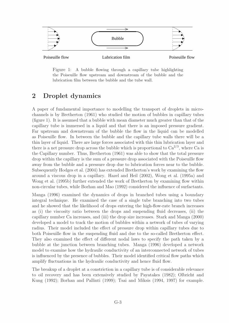
Figure 1: A bubble flowing through a capillary tube highlightingthe Poiseuille flow upstream and downstream of the bubble and thelubrication film between the bubble and the tube wall.

2 Droplet dynamics

A paper of fundamental importance to modelling the transport of droplets in micro-channels is by Bretherton (1961) who studied the motion of bubbles in capillary tubes(figure 1). It is assumed that a bubble with mean diameter much greater than that of thecapillary tube is immersed in a liquid and that there is an imposed pressure gradient.Far upstream and downstream of the bubble the flow in the liquid can be modelledas Poiseuille flow. In between the bubble and the capillary tube walls there will be athin layer of liquid. There are large forces associated with this thin lubrication layer andthere is a net pressure drop across the bubble which is proportional to Ca2/3, where Ca isthe Capillary number. Thus, Bretherton (1961) was able to show that the total pressuredrop within the capillary is the sum of a pressure drop associated with the Poiseuille flowaway from the bubble and a pressure drop due to lubrication forces near to the bubble.Subsequently Hodges et al. (2004) has extended Bretherton’s work by examining the flowaround a viscous drop in a capillary. Hazel and Heil (2002), Wong et al. (1995a) andWong et al. (1995b) further extended the work of Bretherton by examining flow withinnon-circular tubes, while Borhan and Mao (1992) considered the influence of surfactants.

Manga (1996) examined the dynamics of drops in branched tubes using a boundaryintegral technique. He examined the case of a single tube branching into two tubesand he showed that the likelihood of drops entering the high-flow-rate branch increasesas (i) the viscosity ratio between the drops and suspending fluid decreases, (ii) thecapillary number Ca increases, and (iii) the drop size increases. Stark and Manga (2000)developed a model to track the motion of bubbles within a network of tubes of varyingradius. Their model included the effect of pressure drop within capillary tubes due toboth Poiseuille flow in the suspending fluid and due to the so-called Bretherton effect.They also examined the effect of different nodal laws to specify the path taken by abubble at the junction between branching tubes. Manga (1996) developed a networkmodel to examine how the hydraulic conductivity of an interconnected network of tubesis influenced by the presence of bubbles. Their model identified critical flow paths whichamplify fluctuations in the hydraulic conductivity and hence fluid flow.

The breakup of a droplet at a constriction in a capillary tube is of considerable relevanceto oil recovery and has been extensively studied by Payatakes (1982); Olbricht andKung (1992); Borhan and Pallinti (1999); Tsai and Miksis (1994, 1997) for example.

G-3

Figure 2: Some challenging free boundary problems involving movingcontact lines between the oil (shaded) and water phases.

Tice et al. (2004) examined the influence of viscosity on the formation of dropletsin microfluidic channels while Anna et al. (2003); Ganan Calvo and Gordillo (2001)showed how flow focussing (forcing a capillary jet through a narrow orifice) can leadto monodisperse formation of bubbles and droplets. Song et al. (2003) and Thorsenet al. (2001) examined microfluidic formation of droplets at T-junctions while Sugiuraet al. (2001) and co-workers have experimented with different microfluidic geometries todevelop monodisperse droplets.

3 Parameter estimation

A typical microfluidic channel in the network has a length of approximately L = 1 cm anda width and height of around a = 100 µm. A typical flow rate of 1 ml/hr equates to a flowvelocity in such a channel of the order of 1 cm s−1. We take the dynamic and kinematicviscosities for water as µw = 10−3 kg m−1 s−1 and νw = 10−6 m2 s−1. respectively. Thedynamic viscosity of oil is taken to be µo = 10−2 kg m−1 s−1 and the surface tension at

G-4

the interface is assume to be roughly σ ≈ 50 dyn cm−1. From these values the Reynoldsnumber and Capillary number are calculated to be

Re =U a

νw

∼ 1, Ca =µwU

σ∼ 10−2.

Clearly, surface tension effects are very dominant and this leads to some very interesting,but difficult, free boundary problems at the nodes where the oil and water phases meet(figure 2). Due to the time constraints of the Study Group week, we decided not totackle these problems directly, but instead to concentrate on developing a multiphase(nonlinear) generalisation of an electric-circuit theory model. This is described in thesection below.

4 A network model

In this section we consider the flow in two model networks:

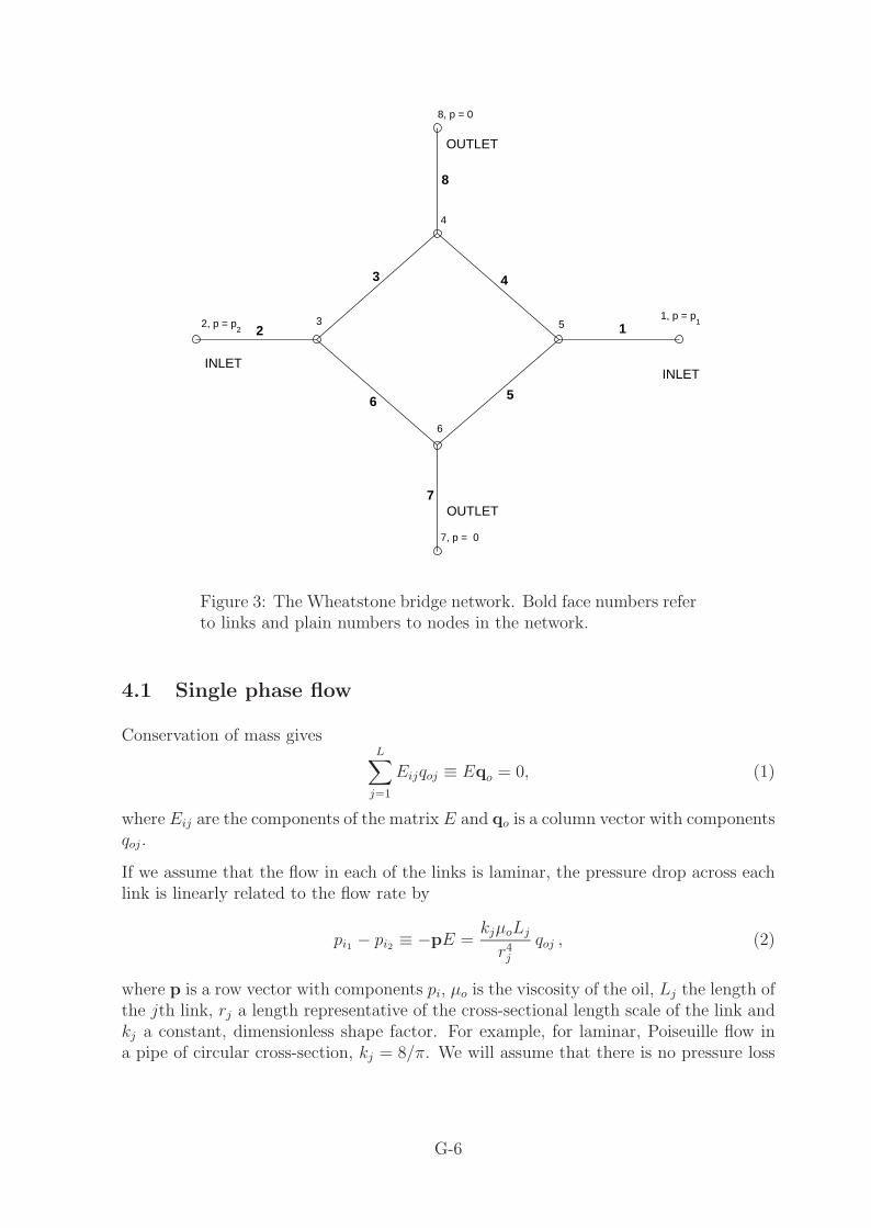
• A ‘Wheatstone bridge’ network, which has two inlets and two outlets, as illustratedin figure 3. This network has just 8 links and 8 nodes and has been studiedexperimentally by Unilever.

• A parallel mixing network, which has three inlets and m+1 outlets for some positivenumber m, as shown in figure 4. This produces droplets from single phase inletflows, and is an example of a possible application of the technology. The networkhas 8m + 5 links and 6m + 6 nodes. Water flows in through inlet node 2, whilstoil enters through inlet nodes 1 and 3. The idea is that oil droplets in water areformed at nodes 6, 11, . . . , 5m + 4, and that compound droplets of oil in water inoil form at nodes 8, 13, . . . , 5m + 5.

The volume flow rates of oil and water in each of the j = 1, 2, . . . , L links are qoj andqwj and the pressure at each of the i = 1, 2, . . . , N nodes is pi. Note that we will assumethat the pressure in each of the phases is equal. The effect of differing fluid pressures,due, for example, to surface tension, could be included in the model at a later date.

We describe the network using an N × L matrix E. If the jth link connects the i1thand i2th nodes, with i1 < i2, then the jth column of E has just two nonzero entries, −1in the i1th row and +1 in the i2th row. The matrix E is therefore sparse with just 2Lnonzero entries. We measure flow rates in each link to be positive in the direction fromthe i1th to the i2th node.

We will consider pressure-driven flows, which is more likely to be the arrangement usedin practice, with pressures prescribed at the I inlet and O outlet nodes and the inlet andoutlet flow rates to be determined.

G-5

1, p = p12, p = p

23

4

5

6

7, p = 0

8, p = 0

INLET INLET

OUTLET

OUTLET

8

1

7

2

5 6

3 4

Figure 3: The Wheatstone bridge network. Bold face numbers referto links and plain numbers to nodes in the network.

4.1 Single phase flow

Conservation of mass givesL∑

j=1

Eijqoj ≡ Eqo = 0, (1)

where Eij are the components of the matrix E and qo is a column vector with componentsqoj.

If we assume that the flow in each of the links is laminar, the pressure drop across eachlink is linearly related to the flow rate by

pi1 − pi2 ≡ −pE =kjµoLj

r4j

qoj , (2)

where p is a row vector with components pi, µo is the viscosity of the oil, Lj the length ofthe jth link, rj a length representative of the cross-sectional length scale of the link andkj a constant, dimensionless shape factor. For example, for laminar, Poiseuille flow ina pipe of circular cross-section, kj = 8/π. We will assume that there is no pressure loss

G-6

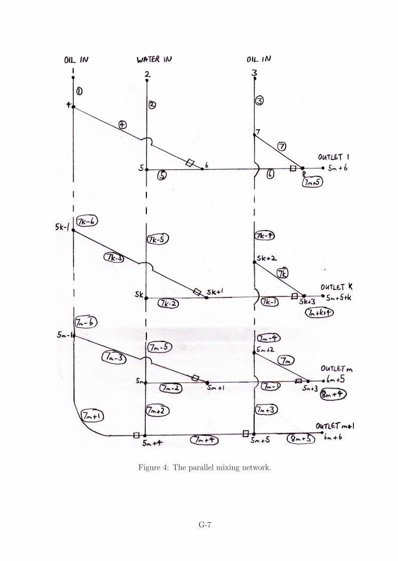
Figure 4: The parallel mixing network.

G-7

across the nodes, although this could be included in the model. Note that the matrix-vector multiplication form of (1) and (2) indicates that representing the network usingthe sparse matrix E is a sensible approach.

There are N −O − I unknown pressures and L unknown flow rates, whilst conservationof mass, (1), provides N −O− I equations, and the dynamical relation (2), L equations.Equations (1) and (2) therefore provide a linear system of N − O − I equations andN − O − I unknowns.

Rather than use the applied pressure as a basis for nondimensionalizing the system, wewill use the capillary pressure pc = 2σ/r due to a hemispherical oil/water meniscus ofradius r, with r a typical cross-sectional channel dimension. The reasons for this willbecome clear in the next section. The flow rate due to this pressure drop in a channel oflength L is qc = 2σr3/kµoL, where k is a typical shape factor. Typically, pc ≈ 1000Paand qc ≈ 4× 10−10m3s−1, in line with the typical values given in section 3. We thereforedefine dimensionless variables

pj =pj

pc

, qoj =qoj

qc

, (3)

in terms of which (1) and (2) become

L∑j=1

Eij qoj ≡ Eqo = 0, (4)

pi1 − pi2 ≡ −pE = Rj qoj, (5)

where

Rj =kj Lj r4

k L r4j

(6)

is the resistance of the jth link. Equations (4) and (5) are equivalent to Kirchhoff’s lawsfor an electrical network, with pressure difference equivalent to voltage difference, andflow rate equivalent to current. It is well known that the linear equations (4) and (5)subject to prescribed inlet and outlet pressures are linearly independent, and thereforehave a unique solution.

Figure 5 shows a typical solution for the Wheatstone bridge network illustrated infigure 3, with unit resistance in each link, driven by unequal inlet pressures. We shouldalso note that if one of the inlet pressures is too low, the flow may reverse and flow outthrough an inlet and possibly in through an outlet. For single phase flow, if we assumethat the outlets are attached to oil reservoirs at zero nominal pressure, this remains anacceptable solution. The situation is different for oil/water flows, as we shall see.

4.2 Oil/water flow

If both oil and water flow into a network and mix, we are faced with all the usualproblems associated with multiphase flow (see, for example, Drew and Passman, 1999).We need models for the forces that the two phases exert upon each other and upon the

G-8

1, p = 12, p = 2 3, p = 1.067

4, p = 0.6

5, p = 0.7333

6, p = 0.6

7, p = 0

8, p = 0

qw = 0, q

o = 0.2667q

w = 0, q

o = 0.9333

qw = 0, q

o = 0.4667 q

w = 0, q

o = −0.1333

qw = 0, q

o = 0.1333q

w = 0, q

o = 0.4667

qw = 0, q

o = 0.6, a = 1

qw = 0, q

o = 0.6, a = 1

INLET

INLET

OUTLET

OUTLET

Figure 5: A typical solution for the flow of oil in the network shownin figure 3.

channel walls. For steady flow, this amounts to knowledge about the rate at which onefluid moves relative to the other, and the frictional pressure gradient in the channel. Inthe work reported here, we make the simplest possible assumption, which is that thefluids do not slip relative to each other, and that the frictional pressure gradient is linearin the two fluid flow rates. Irrespective of these considerations, conservation of mass ateach node is given by

L∑j=1

Eij qoj ≡ Eqo = 0,L∑

j=1

Eij qwj ≡ Eqw = 0. (7)

The linearity of the frictional pressure gradient can be expressed as

pi1 − pi2 ≡ −pE = Rj (qoj + µqwj) , (8)

where µ = µw/µo ≈ 0.1.

In pressure-driven flows, which we study here, we must also specify the pressure at Iinlet and O outlet nodes, as we did for single phase flow. However, at the inlet nodes

G-9

we must also specify the composition of the incoming fluid to be either oil or water.There are N −O− I unknown pressures and 2L unknown flow rates, whilst conservationof mass (7) provides 2(N − O − I) equations, the dynamical relation (8) L equations,and knowledge of the inlet composition a further I equations. The number of unknownstherefore exceeds the number of equations by L−N+O. We can see where this imbalancecomes from by considering a simple network with I inlets and O outlets joined at a singleinterior node. In this case N = I + O + 1 and L = I + O, so that L − N + O = O − 1,and the number of extra equations required depends solely on the number of outlets.The extra equations are required to specify how the fluid phases divide as they leavethe node. This conclusion applies in general to any internal node in a network. If theflow leaves a given node through n links, then n− 1 extra equations must be applied atthat node. There is a simple, and plausible, way of obtaining these extra equations. Wecalculate the total oil and water flow rates into the ith node, Qoi and Qwi, and deducethe mean inlet oil fraction, αi = Qoi/(Qoi + Qwi). The new conditions are that the oilfraction should be αi in each of the links where the flow is directed out of the node. Thekey point is that once we have applied these equations in (n − 1) of the outflow links,applying it in the remaining outflow link is not necessary by conservation of mass (7).This means that these extra conditions, which we note are nonlinear, can be appliedat each node in the network without having to determine a priori which nodes havemore than one link with outflow. The “equal oil fraction” law agrees with the numericalexperiments of Stark and Manga (2000). Some of the constraints associated with tryingto apply different extra conditions are described later in section 6.

It was also felt that we should include the effect of an oil/water meniscus at junctionswhere drops are formed. The capillary pressure due to such a meniscus is around 2σ/rj,where σ is the surface tension. If the magnitude of the pressure drop across the link is lessthan this, no flow occurs. We can build this into the model by including an additionalpressure loss in links where we know a priori that the fluid is exiting into a single phaseflow of the fluid that does not form the continuous phase. We rewrite (8) as

pi1 − pi2 ≡ −pE = Rj (qoj + µqwj) + C sgn (qoj + qwj) for |qoj + qwj| > 0,

|pi1 − pi2| ≤ C for qoj + qwj = 0. (9)

Since we have nondimensionalized pressure on a capillary scale, we expect that C isO(1), and in the following results, we have taken C = 1 when using this modified flowlaw. In fact, we need to smooth out this discontinuous function to be able to use it in anumerical solver. We used

pi1 − pi2 = Rj (qoj + µqwj) + Csgn (qoj + qwj)(1 − e−|qoj+qwj |/qsm

), (10)

with qsm = 10−4. There are other possibilities that could be used as dynamic laws insteadof (10), which are discussed in section 6.

In order to solve the nonlinear system of equations (7) and (10), along with specifiedinlet and outlet pressures and inlet oil fractions (0 or 1), we used Newton iteration,implemented as a MATLAB function. The version of the code that solves for the parallelmixing network is fully annotated, and listed as appendix A. It should be noted that the

G-10

code could be made much more efficient by reusing the Jacobian to give a quasi-Newtonmethod, but we have not pursued this here. Even for a parallel mixing network withm = 100, the largest system tackled here, the solution can be obtained in about 15minutes on a 2.8GHz Pentium IV PC.

Before presenting some results, we should note that for both types of network, whetheror not the effect of oil/water menisci was included, we found no numerical evidence fornon-uniqueness of the solution. When we started by finding the solution for either singlephase oil, single phase water or an oil fraction of 0.5 in each inlet, and then used this asthe initial guess for the situations described below, the solution to which the iterationconverged was always the same. We have not, however, attempted to prove that thesolution is unique, although this is an interesting problem.

4.3 Results for the Wheatstone bridge network

In figure 6 we show the solution when single phase oil enters through node 1 and singlephase water through node 2. Mixing therefore occurs at nodes 4 and 6, but, to beginwith, we have not included the effect of the oil/water meniscus in links 4 and 5 (seefigure 3). In figure 6a, the outlet oil fraction is about 0.22 at node 7 and also, bysymmetry, at node 8. If we reduce the pressure at the water inlet, the water flow ratedecreases, as we would expect, until, when p ≈ 2.5, the water flow rate falls to zero.Only oil then flows through the network, as shown in figure 6b. If we drop the waterinlet pressure further, node 2 becomes an outlet for single phase oil.

Figure 7 shows the analogous results when we include the effect of the oil/water meniscusin links 4 and 5. As we would expect, the pressure losses across these links are higherthan those shown in figure 6, and the water inlet pressure can fall slightly more beforethe flow rate of water falls to zero.

4.4 Results for the parallel mixing network

Figures 8 to 10 show the outlet flow rates and outlet oil fractions for parallel mixingnetworks of various sizes. The effect of the oil/water meniscus in the appropriate links(see figure 4) has been included. In addition, the inlet flow lines for the single phaseoil and water (links 7k − 6, 7k − 5 and 7k − 4 for k = 1, 2, . . . , m and 7m + 1, 7m + 2and 7m + 3 in figure 4) have resistances 100 times smaller than that of each of the linkswithin the network. The reasons for this are discussed in section 5. In each network,the flow rates decrease the further the outlet is from the inlet, as the driving pressure isdecreased by the frictional pressure drop. In addition, the outlet oil fractions decreasealong the network, since the oil outlet flow rates fall more rapidly than the water outletflow rates, as a consequence of the higher viscosity of the oil. As the number of outletsincreases, the outlet conditions appear to converge towards a form that is independentof the number of outlets. This phenomenon could be investigated using an asymptoticapproach valid for large m, which could take the form of an effective medium theory, but

G-11

qw = 6.7, q

o = 2.3, a = 0.26

1, p = 102, p = 5 3, p = 3.7

4, p = 3

5, p = 5.3

6, p = 3

7, p = 0

8, p = 0

qw = 0, q

o = 4.7q

w = 13, q

o = 0

qw = 6.7, q

o = 0 q

w = 0, q

o = −2.3

qw = 0, q

o = 2.3q

w = 6.7, q

o = 0

qw = 6.7, q

o = 2.3, a = 0.26

qw = 0, q

o = 2.5, a = 1

1, p = 102, p = 2.5 3, p = 2.5

4, p = 2.5

5, p = 5

6, p = 2.5

7, p = 0

8, p = 0

qw = 0, q

o = 5q

w = 0, q

o = 0

qw = 0, q

o = 0 q

w = 0, q

o = −2.5

qw = 0, q

o = 2.5q

w = 0, q

o = 0

qw = 0, q

o = 2.5, a = 1

OUTLET

OUTLET

WATERINLET

OIL INLET

OUTLET

OUTLET

WATERINLET

OILINLET

a)

b)

Figure 6: Two solutions for the flow of oil and water in the networkshown in figure 3. In b), the inlet water pressure is too low to driveany flow, and single phase oil leaves the outlet. If p2 < 2.5, singlephase oil would also be driven out of inlet node 2.

G-12

qw = 7.3, q

o = 2.1, a = 0.22

1, p = 102, p = 5 3, p = 3.5

4, p = 2.8

5, p = 5.9

6, p = 2.8

7, p = 0

8, p = 0

qw = 0, q

o = 4.1q

w = 15, q

o = 0

qw = 7.3, q

o = 0 q

w = 0, q

o = −2.1

qw = 0, q

o = 2.1

qw = 7.3, q

o = 0

qw = 7.3, q

o = 2.1, a = 0.22

qw = 0, q

o = 2.25, a = 1

1, p = 102, p = 2.25 3, p = 2.25

4, p = 2.25

5, p = 5.5

6, p = 2.25

7, p = 0

8, p = 0

qw = 0, q

o = 4.5q

w = 0, q

o = 0

qw = 0, q

o = 0 q

w = 0, q

o = −2.25

qw = 0, q

o = 2.25q

w = 0, q

o = 0

qw = 0, q

o = 2.25, a = 1

OUTLET

OUTLET

WATERINLET

OILINLET

OUTLET

OUTLET

WATERINLET

OILINLET

a)

b)

Figure 7: Two solutions for the flow of oil and water in the networkshown in figure 3, including the effect of an oil/water meniscus inlinks 4 and 5. In b), the inlet water pressure is too low to driveany flow, and single phase oil leaves the outlet. If p2 < 2.25, singlephase oil would also be driven out of inlet node 2.

G-13

10 20 30 40 50 60 70 80 90 1000

0.5

1

1.5

2

2.5

3

3.5

4

4.5

5

output number

oil f

low

rate

m=1m=5m=10m=25m=50m=75m=100

Figure 8: The outlet oil flow rates for parallel mixing networks ofvarious sizes. All inlet pressures are equal to 10.

10 20 30 40 50 60 70 80 90 1000

5

10

15

output number

wat

er fl

owra

te

m=1m=5m=10m=25m=50m=75m=100

Figure 9: The outlet water flow rates for parallel mixing networksof various sizes. All inlet pressures are equal to 10.

G-14

we have not investigated this further here. We also found that if the inlet pressure wastoo low, it was not sufficient to drive a flow through the network, as we would expect.

The outlet oil flow rates can be increased by increasing the pressure at the oil inlets.However, for sufficiently high oil inlet pressures, the water is unable to hold back the oil,which flows into the water inlet line through link 5 (see figure 4). This is illustrated infigure 11. Once the inlet pressure at node 2 increases past 13.98, oil flows through node5. Of course, in this case there is now no longer an oil/water meniscus in link 4, butthere is in link 5.

5 Stability of parallel microfluidic networks

As mentioned in the introduction, it may be necessary to operate many microfluidicdevices simultaneously, for example in order to obtain a high production rate of droplets;or to test for the presence of many different chemicals at one time. Instead of utilisinga large number of self-contained microfluidic circuits, the component devices may beconnected in parallel, as shown in figures 4 and 12.

Microfluidic devices connected in parallel share a single fluid supply pump and othersupporting infrastructure. This greatly reduces the overall cost and physical complexityof the system. However, the user can only control the behaviour of the network byadjusting the fluid flow rate at the inlet, Qin, and the pressure at the outlet, pout. It isimportant that each branch of the network should operate reliably with this low level ofcontrol, even if the exact pressure-flow characteristics of the individual branches in thenetwork differ due to variations during the manufacture of the network. Therefore in thefollowing sections we consider how network design and device manufacturing tolerancesaffect the performance of a massively parallel microfluidic network, and show how thestability of networks can be improved.

5.1 A parallel array of nozzles

We will analyse a parallel array of nozzles shown in figure 12. This circuit could beused for a simple droplet production process. The network is made up of N parallelbranches which are fed with fluid from a single low-resistance supply vessel, and draininto a single large output vessel. Each branch contains a single nozzle, connected to themain fluid supply vessel by a channel with resistance Ri, as described by equation (5).The pressure-flow characteristics of the nozzles are represented by nonlinear resistances.The pressure drop across the ith nozzle, ∆p

(f)i , is related to the flux of fluid in the nozzle,

qi, by the expression∆p

(f)i = fi(qi) for i = 1, 2, . . . , N.

We now account for the small variations in the flow characteristics of the channels andnozzles which result from the manufacturing process. We express the resistances Ri andthe functions fi(q) as the sum of the average values, R and f(q) respectively, which are

G-15

10 20 30 40 50 60 70 80 90 1000.1

0.12

0.14

0.16

0.18

0.2

0.22

0.24

0.26

0.28

output number

oil f

ract

ion

m=1m=5m=10m=25m=50m=75m=100

Figure 10: The outlet oil fractions for parallel mixing networks of various sizes. All inletpressures are equal to 10.

5 10 15 20 25 30 35 40 45 500

1

2

3

4

5

6

7

outle

t vol

ume

flow

rate

output number

wateroil

5 10 15 20 25 30 35 40 45 500

0.2

0.4

0.6

0.8

1

oil f

ract

ion

output number

Figure 11: The outlet flow rates and outlet oil fractions for a parallel mixing networkwith m = 50. The water inlet pressure is 10, as is the oil inlet pressure at node 3, whilstthe oil inlet pressure at node 2 is 13.98. For higher pressures at node 2, oil enters thewater inlet flow line through node 5.

G-16

independent of i, and a small correction term which represents the variations betweenthe components:

Ri = R + εRi , fi(q) = f(q) + εfi(q) for i = 1, 2, . . . , N , (11)

where 0 < ε � 1 is a measure of the manufacturing tolerance, and

R =1

N

N∑i=1

Ri , f(q) =1

N

N∑i=1

fi(q) for all q.

Note that the definitions of Ri and fi imply that

N∑i=1

Ri = 0 ,N∑

i=1

fi(q) = 0 for all q.

The mathematical description of the system is straightforward. Conservation of mass inthe network requires

Qin =N∑

i=1

qi. (12)

Because the input and output vessels are assumed to have a very low resistance to flow,the total pressure drop across each branch of the network is equal to the difference ofthe inlet and outlet pressures. Therefore

pin − pout = Ri qi + fi(qi) for i = 1, 2, . . . , N. (13)

We seek a solution of (11)–(13), to determine the qi and pin, using regular perturbationanalysis. We expand the fluxes, qi, and the inlet pressure in powers of ε:

qi = q(0)i + ε q

(1)i + ε2 q

(2)i + . . . (14)

pin = p(0)in + ε p

(1)in + ε2 p

(2)in + . . . (15)

Substituting these expansions into (11)–(13) and collecting the leading order terms, wefind

Qin =N∑

i=1

q(0)i , (16)

p(0)in − pout = Rq

(0)i + f(q

(0)i ). (17)

The leading order problem is solved by an even distribution of the fluxes between thebranches,

q(0)i =

Qin

N, p

(0)in =

RQin

N+ f(Qin/N). (18)

G-17

At the next order, O(ε), the perturbations Ri and fi(q) enter the analysis. Equations for

q(1)i and p

(1)in are found by inserting the expansions (14) and (15) into equations (11)–(13)

and retaining terms of O(ε) only. We find

0 =N∑

i=1

q(1)i , (19)

p(1)in = R q

(1)i + Ri q

(0)i + fi(q

(0)i ) + q

(1)i

(df

dq

) ∣∣∣∣∣q=q

(0)i

. (20)

Solving equations (19) and (20), we obtain

q(1)i = −Ri Qin/N + fi(Qin/N)

R +(

dfdq

)∣∣∣q=(Qin/N)

, p(1)in = 0. (21)

Combining the leading order solution, (18), and the first correction, (21), we have shownthat the flux in the ith branch of the network is described by

qi =Qin

N− ε

Ri Qin/N + fi(Qin/N)

R +(

dfdq

)∣∣∣q=(Qin/N)

+ . . . , (22)

=Qin

N− (Ri − R) Qin/N + (fi(Qin/N) − f(Qin/N))

R +(

dfdq

)∣∣∣q=(Qin/N)

+ . . . . (23)

Equation (23) shows that the differences between the fluxes in the ith branch and theaverage flux q = Qin/N depends on (Ri − R) and (fi(q) − f(q)), as expected. However,(23) also shows (qi − q) may be reduced by making the average channel resistance, R,large. This occurs because the fluid flow divides between the branches according to theoverall flow resistance of the branch. By increasing R, the deviations in the resistance ofthe channels and nozzles become small compared to the overall resistance of the branch,and their effect on the division of the flow will be also small. However, it may onlybe possible to increase the mean resistance R of the vessels whilst keeping errors Ri

of the same order of magnitude by lengthening the channel (not by narrowing). Such arequirement of long input channels may create some difficulties in compact device design.

We can also consider the effect on the network operation of blocking some branches ofa parallel network. If a proportion p (0 ≤ p ≤ 1) of the channels become blocked, thechange in the flux per channel will be

∆q =Qin

N− Qin

N − pN(24)

=Qin

N

(p

1 − p

). (25)

Thus the change in the average flux per channel due to channel-blocking events decreasesas N → ∞. Therefore channel blocking will cause less disruption to the operating regimeof the remaining open channels if N is large.

G-18

(Branchesrepeated)

Flow in

Flux: Qin

vessel(low resistance)

Main output

Pressure:p = pout

Main supplyvessel(low resistance)

Pressure:p = pin

R1

R2

R2

RN−2

RN−1

f1

f2

f3

fN−2

fN−1

fN

Channels Nozzles

RN

q1

q2

q3

qN−2

qN−1

qN

Flux

Flow out

Figure 12: The parallel array of nozzles, analysed in Section 5.1.

G-19

6 Further comments

6.1 Imposing other nodal conditions

pin

p

p

πRin

R

R

Qo, Qw

Qo, qw

0, qw

Figure 13: Imposing other nodal laws: the case when all oil dropletsenter the same preferential outgoing channel.

In the derivation of our two-phase network model in section 4.2, extra conditions wererequired at nodes where flow splitting occurs, to specify how the phases divide as theyleave the node. For the subsequent calculations, the simple condition of equal oil/waterfraction into each outgoing channel was used. However, the work of Manga (1996) revealsthat the equal oil/water fraction is an oversimplification of the droplet dynamics at abifurcation. Indeed, droplet size and structure, viscosity ratio, capillary number as wellas the network vessel properties themselves all have the ability to alter the proportionof droplets entering a particular outgoing channel at a junction.

A natural question to now ask is: can other nodal conditions be imposed in our networkmodel? To test such an idea, we examine whether a nodal law for which every oil dropletis drawn down a single outgoing channel will lead to a consistent set of equations. Forsimplicity, we take a single bifurcating node (figure 13) where the incoming flow is amixed phase of oil droplets and water. The upstream and downstream pressures pin, pand p are set. The incoming oil and water volume flow rates are Qo and Qw respectivelyand the ratio of the two is fixed. Without loss of generality, we assume the pressuredrop into the upper branch (pin − p) is larger than the pressure drop into the lowerbranch (pin − p) and that all the oil droplets are thus drawn into the upper branch (ournew nodal condition). The resistances of the upstream mother vessel Rin, the upper

outgoing vessel R and the lower outgoing vessel R are known and the water phase splitsinto volume flow rates qw and qw in the upper and lower outgoing vessels respectively.

G-20

From the model in section 4, the following system of equations arises:

(pin − π) = Rin(µQw + Qo), (26)

(π − p) = R(µqw + Qo), (27)

(π − p) = Rµqw, (28)

Qw = qw + qw, (29)

where π is the internal pressure at the node itself. The first equation (26) is only requiredto determine the magnitude of the incoming volume flow rates; any possible constraintcan be found from the other equations. Eliminating π from (27) and (28) and solvingfor the water volume flow rate qw in the lower vessel, using (29), leads to

qw =R

µ(R + R)

(µQw + Qo − (p − p)

R

).

This solution is only physically sensible if the water volume flow rate into the loweroutgoing channel is less than the incoming water volume flow rate, qw � Qw. Otherwise,water would have to be drawn in from the upper channel, leading to the water and oilphases travelling in opposite directions there. Of course, qw < 0 is perfectly acceptable,resulting in the lower outgoing channel feeding water into the mixed phase upper channel,qw > Qw (so long as the lower outgoing channel is connected to a water reservoir).Applying the inequality to the expression above leads to the constraint

R

µR

(Qo − (p − p)

R

)� Qw.

This constraint only allows oil droplets to all take the same channel out of the node if

• the pressure drop in the oil-laden channel is large enough compared to otheroutgoing channel (possibly reversing the flow in the other outgoing channel forinstance);

• the resistance in the oil-laden channel (R) is much lower than the other outgoingchannel;

• the viscosity ratio µ is close to unity;

• the oil fraction is not too large (Qo < µQw appears to be a reasonable rule-of-thumb).

Whilst we have approached the nodal condition and necessary constraint from a networkpoint-of-view, it is worth noting that some of these observations above are similar to thosemade by Manga (1996) in terms of droplet dynamics and channel selection.

G-21

6.2 Alternative laws for the flow dynamics in the channels

Our network model is presently based on no-slip between the two phases, leading to alinear relationship between pressure and volume flux through a vessel. For single-phasecarrying vessels this relationship is perfectly valid, but for mixed-phase channel flow largeslip forces and nonlinear pressure-flux relationships must be considered. One example isthat of Bretherton (1961), which applies to long bubbles (of volume exceeding 4πr3/3where r is the cross-sectional radius of the vessel itself) where the viscosity of the bubblecan be neglected. In this case, the pressure-flux relation resembles (Stark and Manga,2000)

Q ∼ ∆P −∑

bubbles∆Pb(Q),

where Q is the mass flux, ∆P is the pressure drop across the vessel and ∆Pb is thepressure drop across each bubble, which is proportional Ca2/3. In fact, the work of Wonget al. (1995b) in polygonal capillary channels suggests in certain regimes the pressure-fluxrelation ∆P ∼ Q2/3. Future extensions to the network model could accommodate thisbehaviour depending on the oil fraction, capillary number, etc. However, it is importantto note that these analyses may predict well the behaviour of gaseous bubbles inside aliquid phase, but not oil droplets, as their internal viscosity is likely to have a significanteffect (see Hodges et al., 2004, for details).

7 Conclusions

By assuming no-slip between the two-phases, Kirchhoff’s laws, which form the basisof electric-circuit theory, can be generalised to model two-phase flow in a microfluidicnetwork of channels. For a network of N nodes and L links (channels), of which I nodesare inputs with pressure and phase composition specified and O are output nodes withpressure specified, L − N + O extra equations are required to explain how the phasesdivide at nodes. These equations must remain consistent with mass conservation of eachphase, possibly leading to constraints. The simplest consistent condition to impose atthe dividing nodes is that the volume fraction of each phase remains equal in each of theoutgoing channels. For n-phase flow, it is straightforward to extend this network theory,imposing only one momentum equation in each channel, leading to (n − 1)(L − N + O)extra equations being needed. As with two-phase flow, imposing an equal volume fractionin each of the outgoing channels for each phase leads to a complete system consistentwith mass conservation of each phase (proof by induction). Preliminary results for aWheatstone bridge and parallel-mixing network have been obtained, although no non-uniqueness in the flow field has been found.

On the issue of network stability, we have shown that by making the overall resistance ofthe branches of a parallel network of microfluidic devices large relative to the expectedvariation of resistance between the branches, the division of the fluid flow across thenetwork will become more uniform. This will allow consistent operation of the nozzles(or other components) in all branches of the network. Due to manufacturing tolerances,

G-22

however, this may only be possible by building long feeding channels, which will provedifficult to fit on to a compact device. We have also shown that large parallel networksare more resilient than small networks to blockages of some network branches. Overall,our work suggests that large parallel networks offer good prospects for boosting theefficiency and reliability of microfluidic circuits.

Microfluidics is clearly an important and growing area of research with many excitingquestions to be answered. At present, we have only had time to examine steady networkflow. The possibilities to look at unsteady drop formation at nodal junctions and theassociated pressure rises and falls over time, which generate feedback through the system,appear some of the exciting challenges for the future.

8 Acknowledgements

We would like to thank John Melrose and Guoping Lian for bringing such an interestingproblem to the Study Group. Many thanks are also due to the organisers for makingthe Study Group week such a highly enjoyable and successful event.

References

S. L. Anna, N. Bontoux, and H. A. Stone. Formation of dispersions using flow focussingin microchannels. Appl. Phys. Lett., 82:364–366, 2003.

A. Borhan and C. F. Mao. Effect of surfactants on the motion of drops through circulartubes. Phys. Fluids A - Fluid Dynamics, 4:2628–2640, 1992.

A. Borhan and J. Pallinti. Breakup of drops and bubbles translating through circularcapillaries. Phys. Fluids, 11:2846–2855, 1999.

F. P. Bretherton. The motion of long bubbles in tubes. J. Fluid Mech., 10:166–188,1961.

D. A. Drew and S. L. Passman. Theory of multicomponent fluids. Applied MathematicalSciences. Springer-Verlag, 1999.

A. M. Ganan Calvo and J. M. Gordillo. Perfectly monodisperse microbubbling bycapillary flow focussing. Phys. Rev. Lett., 87:274501, 2001.

A. L. Hazel and M. Heil. The steady propogation of a semi-infinite bubble into a tubeof elliptical or rectangular cross-section. J. Fluid Mech., 470:91–114, 2002.

S. R. Hodges, O. E. Jensen, and J. M. Rallison. The motion of a viscous drop througha cylindrical tube. J. Fluid Mech., 501:279–301, 2004.

M. Manga. Dynamics of drops in branched tubes. J. Fluid Mech., 315:105–117, 1996.

G-23

W. L. Olbricht. Pore-scale prototypes of multiphase flow in porous media. Ann. Rev.Fluid Mech., 292:71–94, 1995.

W. L. Olbricht and D. M. Kung. The deformation and breakup of liquid-drops in lowReynolds number flow through a capillary. Phys. Fluids A - Fluid Dynamics, 4:1347–1254, 1992.

J. Ouellette. A new wave of microfluidic devices. The Industrial Physicist, 9(4):14–17,2004.

A. C. Payatakes. Dynamics of oil ganglia during immiscible displacement in water-wetporous-media. Ann. Rev. Fluid Mech., 14:365–393, 1982.

H. Song, J. D. Tice, and R. Ismagilov. A microfluidic system for controlling reactionnetworks in time. Angew. Chem. Int. Ed., 42:768–772, 2003.

J. Stark and M. Manga. The motion of bubbles in a network of tubes. Transport inPorous Media, 40:210–218, 2000.

H. A. Stone, A. D. Stroock, and A. Ajdari. Engineering flows in small devices:Microfluidics toward a lab-on-a-chip. Ann. Rev. Fluid Mech., 36:381–411, 2004.

S. Sugiura, M. Nakajima, and M. Seki. Interfacial tension driven monodispered dropletformation from microfabricated channel array. Langmuir, 17:5562–5566, 2001.

T. Thorsen, R. W. Roberts, F. H. Arnold, and S. R. Quake. Dynamic pattern formationin a vesicle-generating microfuidic device. Phys. Rev. Lett., 86:4136–4166, 2001.

J. D. Tice, A. D. Lyon, and R. F. Ismagilov. Effects of viscosity on droplet formationand mixing in microfluidic channels. Analytica Chimica Acta, 507:73–77, 2004.

T. M. Tsai and M. J. Miksis. Dynamics of a drop in a constricted capillary tube. J.Fluid Mech., 274:197–217, 1994.

T. M. Tsai and M. J. Miksis. The effects of surfactants on the dynamics of bubblesnap-off. J. Fluid Mech., 348:349–376, 1997.

H. Wong, C. J. Radke, and S. Morris. The motion of long bubbles in polygonal capillaries.1. Thin-films. J. Fluid Mech., 292:71–94, 1995a.

H. Wong, C. J. Radke, and S. Morris. The motion of long bubbles in polygonal capillaries.2. Drag, fluid pressure and fluid-flow. J. Fluid Mech., 292:95–110, 1995b.

G-24

A MATLAB code to solve for flows in the parallel

mixing network

function [qw, qo] = networkm(m0, alphain0, pin0, valvesin, cont)

% NETWORKM: calculates flow in a parallel mixing network of m0 units.

% The output arguments qw and qo are the m0+1 outlet water and oil

% volume flow rates. There are three inlets with pressures pin0 and

% oil fractions alphain0, and m0+1 outlets at zero pressure.

% If cont==1, use initial guess saved in file networkmdata.mat, as

% provided by the previous run of networkm. If valvesin==1, the

% effect of menisci in the appropriate links is included.

% The water/oil viscosity ratio, mu, the link resistances, R, and

% index numbers of the links that have menisci, valves, are specified

% internally. If the solution cannot be obtained directly, calculate

% the flow for single phase inputs, then set cont=1, and try the

% required values.

global N L e I O alphain pin pout mu R n valves m

if (length(alphain0)~=3)|(length(pin0)~=3)|(m0<1)|...

(any(alphain0>1))|(any(alphain0<0))

disp(’Incorrect input data’)

qw=[]; qo=[]; return

end

alphain = alphain0; pin=pin0;

m = ceil(m0); % number of repeating units

N = 6*m+6; % number of nodes

L = 8*m+5; % number of links

I = 3; % number of inlets

O = m+1; % number of outlets

n = 2*L+N-O-I; % number of unknowns

% The matrix l specifies the 2 nodes joined by each link.

l = zeros(2,L);

l(:,1) = [1; 4]; l(:,2) = [2; 5]; l(:,3) = [3; 7];

l(:,4) = [4; 6]; l(:,5) = [5; 6]; l(:,6) = [6; 8];

l(:,7) = [7; 8];

for k = 2:m

l(:,7*k-6) = [5*k-6; 5*k-1]; l(:,7*k-5) = [5*k-5; 5*k];

l(:,7*k-4) = [5*k-3; 5*k+2]; l(:,7*k-3) = [5*k-1; 5*k+1];

l(:,7*k-2) = [5*k; 5*k+1]; l(:,7*k-1) = [5*k+1; 5*k+3];

l(:,7*k) = [5*k+2; 5*k+3];

G-25

end

l(:,7*m+1) = [5*m-1; 5*m+4]; l(:,7*m+2) = [5*m; 5*m+4];

l(:,7*m+3) = [5*m+2; 5*m+5]; l(:,7*m+4) = [5*m+4; 5*m+5];

for k = 1:m

l(:,7*m+k+4) = [5*k+3; 5*m+5+k];

end

l(:,8*m+5) = [5*m+5; 6*m+6];

% The sparse matrix e allows us to calculate pressure drops across

% links and total flow rates into nodes as a sparse matrix multiplication.

e=spalloc(N,L,2*L);

for i = 1:L

e(l(1,i),i) = -1; e(l(2,i),i) = 1;

end

pout = zeros(1,O); % outlet pressures

mu = 0.1; % water/oil viscosity ratio

R = ones(1,L); % link resistances

% inlet lines have low resistance

R([1:7:7*m-6 2:7:7*m-5 3:7:7*m-4]) = ...

0.01*R([1:7:7*m-6 2:7:7*m-5 3:7:7*m-4]);

valves = [];

if valvesin

% specify links with nonlinear valves

for k = 1:m

valves = [valves 7*k-3 7*k-1];

end

valves = [valves 7*m+1 7*m+4];

end

if cont

load networkmdata % load initial guess

if length(x)~=n

disp(’Stored data is not for this network’)

qw=[]; qo=[];

return

end

else

q = [(1-mean(alphain))*ones(1,L) mean(alphain)*ones(1,L)];

p = zeros(1,N-O-I); % simple initial guess

x = [q p];

end

G-26

nitermax = 50; niter=0;

% Newton iteration to get solution

f0=f(x); nf = norm(f0); nf0 = 1e16;

disp(sprintf(’Initial error norm is %3.3g’,nf))

while (nf>1e-8)&(niter<nitermax)&(nf<nf0)

nf0 = nf; J = jacobian(x,f0);

if isempty(J)

disp(’not physical’), return

end

dx = -J\f0’; x = x+dx’;

% Modify guess so that oil and water flow in the same direction

qw = x(1:L); qo = x(L+1:2*L);

for i = 1:L

if qw(i)*qo(i)<0

if abs(qw(i))<abs(qo(i))

qw(i) = -qw(i);

else

qo(i) = -qo(i);

end

end

end

x(1:L) = qw; x(L+1:2*L) = qo;

f0 = f(x); nf = norm(f0); niter = niter+1;

disp(sprintf(’New error norm is %3.3g’,nf))

end

if (niter<nitermax)&(nf<nf0)

qw = x(1:L); qo = x(L+1:2*L);

if any((qw(L-O:L)<0)|(qo(L-O:L)<0))

disp(’not physical’)

else

output(x); save networkmdata x

end

else

disp(’not converging’)

end

%%%%%%%%%%%%%%%%%%%%%%%%%%%%%%%%%%%%%%%%%%%%%%%%

function f = f(x)

global N L e I O alphain pin pout mu R valves

% extract pressures and flow rates and combine with inlet and outlet values

qw = x(1:L); qo = x(L+1:2*L);

p = [pin x(2*L+1:end) pout];

G-27

f =(e*qw’)’; f = f(I+1:end-O);

% sum of water flow rates is zero at interior nodes

f1 =(e*qo’)’; f = [f f1(I+1:end-O)]; ]

% sum of oil flow rates is zero at interior nodes

f1 = -p*e-(mu*qw+qo).*R; % pressure loss proportional to flow rates

% add in the effect of the valves

qt = qw(valves)+qo(valves); % total volume flow rate

f1(valves) = f1(valves) - fvalves(qt);

f = [f f1];

for i = I+1:N-O

qw0 = e(i,:).*qw; qo0 = e(i,:).*qo;

qwplus = qw0(qw0>0); qoplus = qo0(qo0>0);

% flows into the ith node

qwminus = qw0(qw0<0); qominus = qo0(qo0<0);

% flows out of the ith node

Qw = sum(qwplus); Qo = sum(qoplus); % total flows in

alpha = Qo/(Qo+Qw+eps);

% associated oil fraction -- factor of eps to avoid 0/0

% check to avoid problems associated with zero flow rate

if length(qominus)<length(qwminus)

qominus = qo0(qw0<0);

elseif length(qwminus)<length(qominus)

qwminus = qw0(qo0<0);

end

f1 = qominus-alpha*(qominus+qwminus);

f = [f f1(1:end-1)];

% oil fraction equal to alpha in outlet links

end

f1 = qo(1:I)-alphain.*(qo(1:I)+qw(1:I));

% specify the inlet oil fraction

f = [f f1];

%%%%%%%%%%%%%%%%%%%%%%%%%%%%%%%%%%%%%%%%%%%%%%%%

function J = jacobian(x0,f0)

global n L

% calculate the Jacobian associated with f0 at x=x0.

del = 1e-8; J = zeros(n,n);

dir = sign(sign(x0(1:L)) + sign(x0(L+1:2*L)));

dir = [dir dir ones(1,n-2*L)];

% we calculate dir to stop the perturbation of x0 changing the sign

% of a flow rate

for j = 1:n

G-28

del1 = dir(j)*del;

x0(j) = x0(j)+del1;

f1 = f(x0);

if length(f1)~=n

J = []; return

else

J(:,j) = (f1-f0)’/del1;

x0(j) =x0(j)-del1;

end

end

%%%%%%%%%%%%%%%%%%%%%%%%%%%%%%%%%%%%%%%%%%%%%%%%

function output(x)

global pin pout L I O N e X Y m

% plot solution

qw = x(1:L); qo = x(L+1:2*L);

alpha = [];

for j=L-O+1:L

alpha = [alpha qo(j)/(qw(j)+qo(j))];

end figure(100),clf subplot(2,1,1)

plot(1:m+1,qw(end-m:end),’b-x’,1:m+1,qo(end-m:end),’r.-’)

legend(’water’,’oil’,-1),ylabel(’outlet volume flow rate’) XLim([1

m+1]),xlabel(’output number’) subplot(2,1,2),plot(1:m+1,alpha,’k.-’)

ylabel(’oil fraction’) xlabel(’output number’),XLim([1 m+1])

%%%%%%%%%%%%%%%%%%%%%%%%%%%%%%%%%%%%%%%%%%%%%%%%

function dp = fvalves(qt)

% the pressure drop in links with a meniscus

dQ = 0.0001; % a small factor to give almost a step function.

dp = sign(qt).*(1-exp(-abs(qt)/dQ));

G-29