Flow and solute transport around injection wells through a single, growing fracture

$Page 1: Flow and solute transport around injection wells through a single, growing fracture$
Advances in Water Resources 26 (2003) 803–813

www.elsevier.com/locate/advwatres

Flow and solute transport around injection wellsthrough a single, growing fracture

Steven L. Bryant a,*, Ramoj K. Paruchuri a, K. Prasad Saripalli b

a Department of Petroleum and Geosystems Engineering, The University of Texas at Austin, Austin, TX 78712, USAb Pacific Northwest National Laboratory, Richland, WA 99352, USA

Received 22 November 2002; received in revised form 15 May 2003; accepted 23 May 2003

Abstract

During deep-well injection of liquids, the formation around an injection well is often fractured due to an imbalance between the

injection pressure and the minimum horizontal rock stress opposing fracturing. The resulting fractures can grow during injection,

which may span over several months to years. Earlier studies reported on solute transport in a single fracture in low permeability

fractured media, assuming that transport into the formation perpendicular to the face of the fracture is mediated by diffusion alone.

This may be valid for flow under natural gradients through fractured formations of low permeability. In contrast, due to the high

rates of injection through a fractured injection well, both advection and dispersion play an important role in the spread of con-

taminants around a fractured injection well. We present a model for the flow and reactive solute transport profiles around fractured

injection wells, through a single, two-winged vertical fracture created by injection at high rates and/or pressures and growing with

time. The fracture, of constant height and infinite conductivity, serves as a line source injecting fluids into the formation perpen-

dicular to its face via a uniform leak-off, resulting in an elliptical water flood front confocal with the fracture. Flow and solute

transport within the elliptical flow domain is formulated as a planar (two-dimensional) transport problem, described by the ad-

vection–dispersion equation in elliptical coordinates including retardation and 1st order radioactive nuclear decay processes. Results

indicate that transport at early times depends strongly on location relative to the fracture. Retardation has a more pronounced

influence on transport for the cases where advection is significant; whereas 1st order radioactive nuclear decay process is inde-

pendent of advective velocity. Flow and transport around an injection well with a vertical fracture exhibits important differences

from radial transport that neglects the presence of the fracture, and also from transport from a fracture of constant length. The

model and findings presented have applications in the calculation of the fate and transport of contaminants around fractured in-

jectors and modeling the resulting contaminant plumes down stream of the wells. Further, the model also serves as a basis for

modeling enhanced remediation of contaminated rock via injection well fracturing, a recently demonstrated technology.

� 2003 Elsevier Ltd. All rights reserved.

Keywords: Injection wells; Growing fracture; Elliptical flow field; Solute transport

1. Introduction

The objective of this paper is to model single-phase

flow and solute transport around a single, two-winged

vertical fracture, growing around an injection well. In

applications involving the deep-well injection of waste-

waters, oil-field produced waters and hazardous/nuclear

liquid wastes [7,24], the formation around the injectionwell is fractured, due to the imbalance between the in-

*Corresponding author. Tel.: +1-512-471-3250.

E-mail addresses: [email protected] (S.L. Bryant),

[email protected] (R.K. Paruchuri), [email protected]

(K. Prasad Saripalli).

0309-1708/03/$ - see front matter � 2003 Elsevier Ltd. All rights reserved.

doi:10.1016/S0309-1708(03)00065-4

jection pressure and the minimum horizontal rock stress

opposing fracturing. Length of such fractures grows

with the duration of injection, which may span over

several months to years.

There have been a number of theoretical and exper-

imental studies reported, which focused on the nature of

solute transport in a single fracture in low permeability

fractured media (usually in clay-rich aquitards). Ana-lytical solutions for solute transport in an idealized

fracture in a homogeneous porous medium were ob-

tained by reducing the two dimensional problem to two

coupled one-dimensional problems, namely flow along

the fracture and perpendicular to its face [9–

12,17,18,23,25]. There have been relatively fewer models

mail to: [email protected]

Nomenclature

a1 major axis of water flood ellipse (L)

b1 minor axis of water flood ellipse (L)aR minor axis of the elliptical zone extending to

the far-field (L)

bR major axis of the elliptical zone extending to

the far-field (L)

C concentration (ML�3)

C0 injected solute concentration (ML�3)

di position vector along i (L)D dispersion coefficient (L2T�1)Da DamKohler Number

D dispersion tensor (L2T�1)

E Young�s modulus (ML�1T�2)

hf formation thickness (L)

I injectivity (iw=Pw � PR) (M�1L4T)

iw volumetric flow rate (L3T�1)

K constant in the fracture growth power law

functionk formation permeability (L2)

kr radioactive nuclear decay constant (T�1)

Lf fracture half-length (L)

Lf init initial fracture half-length (L)

Lf0 initial fracture half-length (L)

n exponent in the fracture growth power law

function

P1 well flowing pressure (ML�1T�2)Pw bottom hole pressure (ML�1T�2)

PR far field, average reservoir pressure

(ML�1T�2)

Pe Peclet number

Pe� flux-dependent Peclet number

DP1 difference in pressure between water flood

and far-field boundaries (ML�1T�2)

DP2 difference in pressure between cooled frontand water flood front (ML�1T�2)

DP3 pressure difference between the boundary of

fracture and cooled front (ML�1T�2)

DPf pressure increase between the well bore and

fracture tip (ML�1T�2)

DPs pressure increase due to particle plugging of

fracture face (ML�1T�2)

Q flux (L2T�1)R retardation factor

rz radius of water flood zone (L)

rc radius of cooled flood zone (L)

rf radius of extending edge of the fracture

(smaller value of h and Lf ) (L)

s position vector

Sor residual oil saturationSwi irreducible water saturation

t time (T)

u darcy flux (LT�1)

U rock surface energy (MT�2)

Vw volume of water flood zone (L3)

Vc volume of cooled flood zone (L3)

Wi cumulative rate of water injected (L3)

Xgr specific heat of mineral grains (L�1T�2K�1)Xo specific heat of oil (L�1T�2K�1)

Xw specific heat of water (L�1T�2K�1)

x distance along Cartesian longitudinal axis (L)

y distance along Cartesian transverse axis (L)

z distance along depth of injection (L)

/T total formation porosity

/E ½/Tð1� Sor � SwrÞ� effective formation poros-

ityn elliptical coordinate

qgr density of mineral grains (ML�3)

qo density of oil (ML�3)

qw density of water (ML�3)

g elliptical coordinate

r1 total earth stress at the extending end of the

fracture (ML�1T�2)

ðrHÞmin minimum horizontal rock stress opposingfracture (ML�1T�2)

Dr1T change in average interior stress due to dif-

ference in temperature (ML�1T�2)

Dr1P change in average interior stress due to dif-

ference in pressure (ML�1T�2)

s tortuosity

k filtration coefficient (L�1)

l viscosity (ML�1T�1)m Poisson�s ratio

Subscripts

o Oil

gr grains

w waterH horizontal

f fracture

s skin damage

R far field

r residual

804 S.L. Bryant et al. / Advances in Water Resources 26 (2003) 803–813

reported which specifically address the flow and trans-

port around fractured injection wells. Feenstra et al. [8]

provided analytical solutions for the problem of radial

flow around a fractured injection well, ignoring longi-

tudinal dispersion within the fracture and advection–

dispersion perpendicular to the fracture face. Chen [4]

and Chen and Yates [5] presented analytical solutions to

the same problem considering longitudinal dispersion.

S.L. Bryant et al. / Advances in Water Resources 26 (2003) 803–813 805

A critical assumption of the reported analytical

models is that transport into the formation perpendic-

ular to the face of the fracture is mediated by diffusion

alone. This assumption may be valid in the case of flow

through fractured media under natural gradients informations of low permeability. In contrast, the high

rates of injection through a fractured injection well en-

sure that the area of review (defined as the planar area

around the injection well contacted by the injected fluid)

spreads around the well by advection, over several

hundred meters [2,3,6]. The rate of leak-off of injected

wastes perpendicular to the fracture also can be signifi-

cant. As a result, both advection and dispersion play animportant role in the spread of contaminants around a

fractured injection well.

Further, the analytical solutions reported for radial

flow problems [5,8] are applicable for flow around an

injector through a planar, horizontal fracture, as is the

case of water wells intersecting a fracture in a fractured

medium. In contrast, during injection well fracturing,

the vertical fracture grows as a line source in the planview. We present here solutions suitable for modeling

the water flood and solute concentration profiles

around a single, two-winged vertical fracture, which

grows around an injection well. Principal differences

between the present work and the earlier models are as

below:

(1) The fracture considered here is a two-winged, verti-cal fracture of constant height and infinite conduc-

tivity, created by injection at high rates and/or

pressures around an injection well.

(2) The fracture serves as a line source injecting fluids

into the formation perpendicular to its face via a

uniformly distributed leak-off [13,16].

(3) The water flood front around a fracture is elliptical,

rather than radial, in plan view.(4) Advection and longitudinal dispersion within the

matrix govern the solute transport within the ellipti-

cal flow domain growing around the fracture.

(5) Results are given both for static and growing frac-

tures.

It has been widely observed in the petroleum engi-

neering and hydrologic literature that the fracturesaround an injection well indeed develop as single, ver-

tical fractures. The linearity and symmetry of fracture

around the well are idealizations, to render the problem

mathematically tractable.

2. Fracture growth around injection wells

When injection pressures are sufficient to overcome

the minimum horizontal stress within the formation

rock around the wellbore, fractures are initiated in the

adjacent formation. Further, injection of cold water into

a high temperature reservoir can induce thermal stresses

in the near wellbore region, which facilitate fracturing.

This is termed �thermally induced fracturing�. Formationof fractures around the wellbore, which serve as highpermeability injection channels; can significantly facili-

tate the additional injection of water. The bottom hole

injection pressure required to maintain a fracture di-

vided by the reservoir depth is known as the fracture

gradient [22]. When water injection is conducted above

the fracture gradient, the injection wells tend to be

self-stimulating due to the fractures induced by the

temperature and pressure gradients associated with in-jection. The growth of these fractures is well docu-

mented [14–16,22]. Fracturing of wells is also employed

as a well stimulation mechanism as their existence will

counteract the damage incurred from the particle and oil

droplet deposition.

Fracture propagation due to injection is further fa-

cilitated by the difference between water temperature

and the in situ formation temperature with injectiontemperature less than the formation temperature. Such

thermally induced stresses could result in fracture

propagation at pressures smaller than typical formation

parting pressures. The fracture geometry and propaga-

tion rate strongly depend on the formation properties,

injection rate, the quality and chemistry of the water,

and any filtration of colloids from the injection water.

Modeling of fracture formation around injection wells,upon which the present work is based, is briefly dis-

cussed in the following sections. A more complete dis-

cussion of the same can be found in Perkins and

Gonzalez [15,16], Schechter [22] and Saripalli et al. [20].

The Nomenclature section at the end of this paper de-

scribes the notation of variables and symbols used in

this paper.

During water injection, a fracture will be initiated inthe near wellbore region, only when the well flowing

pressure ðP1Þ exceeds the sum of opposing earth stress

ðr1Þ and the rock surface energy contribution opposing

rupture, satisfying the following condition [16]:

P1 ¼ r1 þffiffiffiffiffiffiffiffiffiffiffiffiffiffiffiffiffiffiffiffiffiffi

pUE2ð1� m2Þrf

sð1aÞ

r1 ¼ ðrHÞmin þ Dr1T þ Dr1P ð1bÞ

During the initial stage of injection into an unfractured

formation, when the fracture gradient is insufficient to

initiate a fracture, the cooled and water flood zonesaround the injection well grow radially outward. How-

ever, once the injection pressures exceed the fracture

gradient and a fracture is initiated, the cooled and water

flood fronts grow from radial to increasingly elliptical

patterns, with a linear fracture aligned along the major

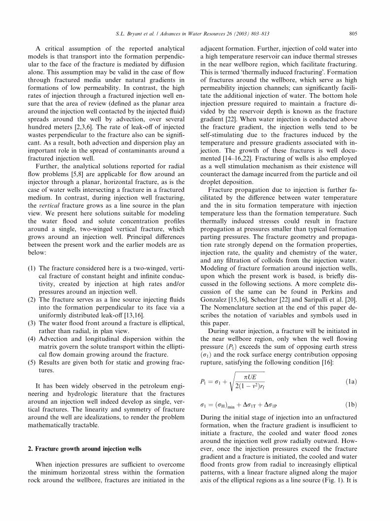
axis of the elliptical regions as a line source (Fig. 1). It is

Cooled front

Water flood front

Direction of min. horizontal stress

Lf

Injection well

Fracture

Fig. 1. Plan view of the flow-field around a growing, two-winged

fracture growing due to injection.


well established that the pressure profiles around the

well bore will be significantly different between the el-

liptical and radial geometries.Once a fracture is initiated, it will propagate as long

as the fracture extension criterion (Eq. (1a)) is satisfied.

The cooled region during this fracture growth can be

approximated as an elliptical zone confocal with the

fracture. The water flood zone is similarly represented as

a larger outer ellipse also confocal with the fracture. The

cooled front is smaller and contained within the water

flood front, since the convective heat transfer throughthe formation is retarded relative to the advective water

flow by the transfer of heat from the rock (Fig. 1). The

fracture grows as the cooled and water flood regions

grow as a result of water injection, and the length of the

fracture (2Lf ) is a function of the dimensions of these

elliptical regions.

During both radial injection and fractured injection,

the bottom hole pressure (Pw) will be equal to the sum ofthe far-field reservoir pressure (PR), and a series of

pressure increases due to the resistance to flow offered

between the wellbore and far-field radius:

Pw ¼ PR þ DP1 þ DP2 þ DP3 þ DPs þ DPf ð2Þ

Eq. (2) subdivides the overall flow resistance into a series

of resistances between successive constant pressureboundaries from the far-field to the injection well. These

resistances include a pressure increase at the boundaries

of cooled and water flood fronts (i.e., DP1 þ DP2 þ DP3)a pressure increase due to perforations (DPf ) and due to

the �skin resistance� near the well, which is a result of

formation damage by suspended particles (DPs). Calcu-lation of these individual pressure terms was discussed in

detail earlier [16,20].Perkins and Gonzalez [16] present a detailed analysis

of how the fracture half-length grows, consistent with its

dependence on the dimensions of the elliptical cooled

and water flood regions, and with Eq. (2). In their

analysis, Perkins and Gonzalez [16] demonstrate that

both the left hand side and right hand side terms of Eq.

(2), i.e., the flowing well pressure and the resisting earth

stress respectively, also critically depend on the dimen-

sions of the elliptical zones. The flowing pressure Pw is

calculated as a sum of a series of pressure increases from

the injection well, as shown in Eq. (2). The pressureincrease terms (DP1, DP2 etc.) depend on the dimensions

of the region in which the pressure increase is calculated.

We adapt the analysis of Perkins and Gonzalez [16] for

the calculation of Pw and r1 with time, and also the re-

sulting fracture length as a function of time. For ex-

ample, in the case of an initially water saturated

formation, the pressure rise DP1 is calculated at steady-

state as

DP1 ¼ iwlw lnð2rf=a1 þ b1Þ=ð2pkhfÞ ð3ÞThe approach presented by Perkins and Gonzalez [16] is

used to calculate the thermal stress and poroelastic stress

profiles during injection. At each time step, the current

values of P1 and r1 are compared to test if Eq. (1) issatisfied. If this condition is met, a fracture will be ini-

tiated and the fracture half-length is calculated as a

function of time, and the thermal and pore pressure

stresses induced. We have presented a complete analysis

of the fracture growth phenomenon around an injection

well injecting particle-laden waters [20]. In the present

work, we focus on modeling the water flood and solute

concentration profiles around the fractured injectionwells, assuming the fracture length––time relationship to

be known a priori.

2.1. Equations governing flow of fluids around the fracture

We seek solutions to model the flow and solute mass

transport profiles around an injection well, due to in-

jection through a single vertical fracture that is growing

with time. If water of constant viscosity is injected into avertical linear, two-winged fracture, the water flood

front will propagate outward, such that its outer

boundary at any time can be described as an ellipse that

is confocal with the fracture [13,16].

With the approximation of the water flood and

cooled flood zones growing as concentric elliptical cyl-

inders around the injection well, the total volumes of

water flood (Vw) and cooled flood (Vc) zones at any time tafter the initiation of injection are calculated as

Vw ¼ Wi

/Tð1� Sor � SwiÞð4Þ

and

Vc ¼qwXwWi

qgrXgrð1� /TÞ þ qwXw/Tð1� SorÞ þ qoXo/TSor

ð5Þwhere Wi , the cumulative volume of water injected at a

constant rate iw for time t, is equal to iwt. When there is

no fracture, the radii of the cooled and water flood


fronts are obtained as rc ¼ffiffiffiffiffiffiffiffiffiffiffiffiffiffiVc=phf

pand rw ¼

ffiffiffiffiffiffiffiffiffiffiffiffiffiffiVw=phf

prespectively. In the presence of a fracture of length 2Lf ,the major and minor axes dimensions of the water flood

ellipse (a1 and b1) can be obtained as

af ¼ LfffiffiffiffiffiF1

p�þ 1=

ffiffiffiffiffiF1

p �=2

bf ¼ LfffiffiffiffiffiF1

p�� 1=

ffiffiffiffiffiF1

p �=2

ð6aÞ

where

F1 ¼2Vw

pL2f hfþ 1

2

ffiffiffiffiffiffiffiffiffiffiffiffiffiffiffiffiffiffiffiffiffiffiffiffiffiffiffiffiffiffi4Vw

pL2f hf

� �2

þ 4

sð6bÞ

Eqs. (4)–(6) can be solved to determine the location of

the elliptical water flood (or liquid waste) front as a

function of injection time and the growing fracture

length.

The fracture can be approximated as an infinite

conductivity source, if the flow resistance in the fracture

itself is negligible compared to the flow resistance be-

tween the far-field boundary and the fracture surface.For such an infinite conductivity fracture, the fracture-

formation boundary is a constant pressure surface, and

the fluid pressure distribution in the formation can be

obtained by solving Laplace�s equation in elliptical co-

ordinates ðn; gÞ, which are related to the physical space

by

x ¼ Lf cosh n cos g ð7aÞ

y ¼ Lf sinh n sin g ð7bÞ

z ¼ z ð7cÞThe coordinate n that defines an isobaric elliptical sur-

face is related to the axes of the water flood ellipse by

n ¼ � 1

2ln

a1 � b1a1 þ b1

ð8Þ

As n approaches 0, the ellipse approaches the line source(fracture) and as n approaches values 1, the ellipse

approaches a circle of radius Lf cosh2 n.

Laplace�s operator in elliptical coordinates is

r2P ¼ 1

h2o2P

on2

�þ o2P

og2þ h2

o2Poz2

h ¼ Lf

ffiffiffiffiffiffiffiffiffiffiffiffiffiffiffiffiffiffiffiffiffiffiffiffiffiffiffiffiffiffiffisinh2 n þ sin2 g

q ð9Þ

Further, since pressure (P ) depends only on n and isindependent of g and z [26], Laplace�s equation reduces

to

o2P

on2¼ 0 ð10Þ

which, upon integration between the far-field and the

line source boundaries yields the pressure distribution:

P ðnÞ ¼ Pw � ðPw � PRÞnnR

ð11Þ

The flux Q ¼ iw=hf leaving the fracture line source is [13]

Q ¼ 2pkl

Pw � PR

ln aRþbRLf

� � ¼ 2pkl

Pw � PRnR

ð12Þ

Here aR and bR refer to the axes of the ellipse defining

the far-field. Eqs. (9)–(12) relates the injection rate and

pressure distribution within the growing elliptic flowdomain. For a constant injection rate iw, we see that theinjection pressure Pw decreases as the fracture grows:

Pw � PR ¼ iwhf

l2pk

lnaR þ bR

Lf

� �

Solute transport in this flow domain is described in the

following sections.

2.2. Equations governing transport of solutes

The general advection–dispersion equation for mass

transport in porous media is given as

/E

oCot

þr � ðuC �DrCÞ ¼ 0 ð13Þ

where u is the darcy flux and D is the dispersion tensor.

Eq. (13) must be formulated in elliptical coordinates in

order to solve for solute transport in the water flood

zone around the linear fracture, which serves as a line

source of injectate. For two-dimensional flow, gradientalong z is zero [1,13]. In planar (i.e., two-dimensional)

elliptical coordinates we have the following:

rs ¼ dn

hoson

þ dg

hosog

ð14aÞ

r2s ¼ 1

h2o2s

on2

�þ o2sog2

�ð14bÞ

r � v ¼ 1

h2o

onðhvnÞ

�þ o

ogðhvgÞ

�ð14cÞ

where di are unit vectors, h ¼ Lfffiffiffiffiffiffiffiffiffiffiffiffiffiffiffiffiffiffiffiffiffiffiffiffiffiffiffiffiffiffiffisinh2 n þ sin2 g

qand

2Lf is the distance between the foci of the ellipse, equal

to the length of the fracture. For a growing fracture, Lfis an increasing function of time, determined from

considerations in the preceding section, and we write

Lf ¼ Lf0LDðtÞ assuming Lf0 as non-zero initial fracture

length for any given time.

Flow from a line source in a homogeneous plane is

only along streamlines of constant g, whence

u ¼ � klrP ¼ � k

hloPon

dn ð15Þ

Using Eqs. (11) and (12), we find

u ¼ 1

hiw2phf

dn

For convenience, we use the darcy flux at the midpoint

of the initial fracture to define a reference speed u0 as


u0 ¼ juðn ¼ 0; g ¼ p=2Þj ¼ 1

Lf0

iw2phf

ð16Þ

Thus we have

u ¼ u0Lf0h

dn ¼u0

LDðtÞffiffiffiffiffiffiffiffiffiffiffiffiffiffiffiffiffiffiffiffiffiffiffiffiffiffiffiffiffiffiffisinh2 n þ sin2 g

q dn

Assuming that dispersion is significant only in the di-

rection of flow, i.e. along a streamline, the transport

equation in elliptical coordinates reduces to

/E

oCot

þ Lf0u0h2

oCon

� Dh2

o2C

on2¼ 0 ð17Þ

where D is the longitudinal dispersion coefficient givenby, D ¼ aLjuj ¼ aLu0Lf0=h, aL being the longitudinal

dispersivity. Because the darcy flux changes with posi-

tion along a streamline and with time in the case of a

growing fracture, the dispersion coefficient D also is a

function of time and space. Thus it is convenient to

separate an invariant ratio of length scales intrinsic to

the problem from the time- and space-dependent aspects

of advection and dispersion.Defining a Peclet number Pe, and a flux-dependent

Peclet number Pe� as

Pe ¼ Lf0aL

and Pe� ¼ u0Lf0D

¼ haL

¼ LfaL

ffiffiffiffiffiffiffiffiffiffiffiffiffiffiffiffiffiffiffiffiffiffiffiffiffiffiffiffiffiffiffisinh2 n þ sin2 g

q

¼ Lf0aL

LDðtÞffiffiffiffiffiffiffiffiffiffiffiffiffiffiffiffiffiffiffiffiffiffiffiffiffiffiffiffiffiffiffisinh2 n þ sin2 g

q

¼ PeLDðtÞffiffiffiffiffiffiffiffiffiffiffiffiffiffiffiffiffiffiffiffiffiffiffiffiffiffiffiffiffiffiffisinh2 n þ sin2 g

qrespectively, and a characteristic advective time scale t0by

t0 ¼/ELf0u0

¼ 2p/EL2f0hf

iw

we have

ðLDðtÞÞ2ðsinh2 n þ sin2 gÞ oCotD

þ oCon

� 1

Peffiffiffiffiffiffiffiffiffiffiffiffiffiffiffiffiffiffiffiffiffiffiffiffiffiffiffiffiffiffiffisinh2 n þ sin2 g

qLDðtÞ

o2C

on2¼ 0

ðvLDðtÞÞ2oCotD

þ oCon

� 1

vLDðtÞPeo2C

on2¼ 0

ð18Þ

where tD ¼ t=t0 and vðn; gÞ ¼ffiffiffiffiffiffiffiffiffiffiffiffiffiffiffiffiffiffiffiffiffiffiffiffiffiffiffiffiffiffiffisinh2 n þ sin2 g

q. Eq. (18)

shows that the transport becomes less dispersive with

increasing distance from the fracture and as the fracturelength increases. For the case of a growing fracture, the

half-length Lf changes with time; our approach for

handling this is described below.

It is important to note that, for systems with a dy-

namically changing extent of the injection boundary,

such as the present case of a growing fracture, Peclet

number is not constant with time nor with position. The

dispersion coefficient is a function of the fluid flux: Dincreases as u0 increases, following a power law [19].

Consequently, taking this dependence into account leads

to Pe� increasing when Lf increases, as will be illustratedbelow.

Eq. (18) is readily generalized to accommodate a re-

tardation factor and radioactive nuclear decay terms:

ðvLDðtÞÞ2RoCotD

þ oCon

� 1

vLDðtÞPeo2C

on2¼ � h2

u0Lf0/krRC

ð19Þ

where R is a dimensionless retardation factor RP 1 and

kr is the radioactive nuclear decay constant. The

(�krRC) term in the Eq. (19) corresponds to the as-

sumption of radioactive nuclear decay of the species in

flowing and sorbed phases. For this example we may

define a characteristic radioactive nuclear decay time tras tr ¼ 1=kr and a Damkohler number as Da ¼ t0=tr,yielding

ðvLDðtÞÞ2RoCotD

þ oCon

� 1

vLDðtÞPeo2C

on2

¼ �DaðvLDðtÞÞ2RC ð20Þ

At any given time, length of the fracture (Lf ) within theprofile, which is a required input for the present mass

transport solution, is obtained according to the proce-

dure explained earlier [20].

For convenience we assume injection into the well at

a constant rate. This translates to a constant flux

boundary condition on Eq. (20). Further, waste liquids

usually are injected for a finite duration t0. These con-ditions are formulated as

Cðn; 0Þ ¼ Ci ð21aÞ

Cð0; tÞ ¼ C0; 06 t6 t0 ð21bÞ¼ 0; t > t0 ð21cÞ

oCon

ð1; tÞ ¼ 0 ð21dÞ

where Ci is the initial concentration of the solute in the

formation; typically Ci ¼ 0. An analytical solution to

Eqs. (20) and (21) is difficult, due to the dependence of

coefficients in advection and dispersion terms on n and g(via h). As such, we solve Eq. (20) subject to (21) along

selected streamlines (g¼ constant) using a finite differ-

ence numerical scheme. It should be noted that the re-

sulting solution describes the flow and contaminant

transport around a static fracture. Presented below is its

extension to the case of a growing (dynamic) fracture.

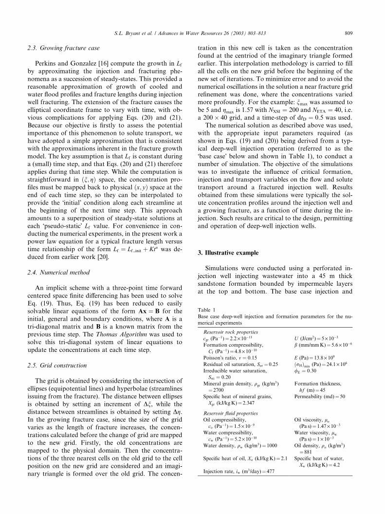
Table 1

Base case deep-well injection and formation parameters for the nu-

merical experiments

Reservoir rock properties

cgr (Pa�1)¼ 2.2 · 10�11 U (J/cm2)¼ 5 · 10�3Formation compressibility,

Cf (Pa�1)¼ 4.8 · 10�10

b (mm/mmK)¼ 5.6 · 10�6

Poisson�s ratio, m ¼ 0:15 E (Pa)¼ 13.8· 109Residual oil saturation, Sor ¼ 0.25 ðrHÞmin (Pa)¼ 24.1· 106Irreducible water saturation,

Swi ¼ 0:20

/E ¼ 0:30

Mineral grain density, qgr (kg/m3)

¼ 2700

Formation thickness,

hf (m)¼ 45

Specific heat of mineral grains,

Xgr (kJ/kgK)¼ 2.347

Permeability (md)¼ 50

Reservoir fluid properties

Oil compressibility,

co (Pa�1)¼ 1.5· 10�9Oil viscosity, lo

(Pa s)¼ 1.47· 10�3Water compressibility,

cw (Pa�1)¼ 5.2 · 10�10Water viscosity, lw

(Pa s)¼ 1· 10�3Water density, qw (kg/m3)¼ 1000 Oil density, qo (kg/m

3)

¼ 881

Specific heat of oil, Xo (kJ/kgK)¼ 2.1 Specific heat of water,

Xw (kJ/kgK)¼ 4.2

Injection rate, iw (m3/day)¼ 477


2.3. Growing fracture case

Perkins and Gonzalez [16] compute the growth in Lfby approximating the injection and fracturing phe-

nomena as a succession of steady-states. This provided areasonable approximation of growth of cooled and

water flood profiles and fracture lengths during injection

well fracturing. The extension of the fracture causes the

elliptical coordinate frame to vary with time, with ob-

vious complications for applying Eqs. (20) and (21).

Because our objective is firstly to assess the potential

importance of this phenomenon to solute transport, we

have adopted a simple approximation that is consistentwith the approximations inherent in the fracture growth

model. The key assumption is that Lf is constant duringa (small) time step, and that Eqs. (20) and (21) therefore

applies during that time step. While the computation is

straightforward in ðn; gÞ space, the concentration pro-

files must be mapped back to physical ðx; yÞ space at theend of each time step, so they can be interpolated to

provide the �initial� condition along each streamline atthe beginning of the next time step. This approach

amounts to a superposition of steady-state solutions at

each �pseudo-static� Lf value. For convenience in con-

ducting the numerical experiments, in the present work a

power law equation for a typical fracture length versus

time relationship of the form Lf ¼ Lf init þ Ktn was de-

duced from earlier work [20].

2.4. Numerical method

An implicit scheme with a three-point time forward

centered space finite differencing has been used to solve

Eq. (19). Thus, Eq. (19) has been reduced to easily

solvable linear equations of the form Ax ¼ B for the

initial, general and boundary conditions, where A is atri-diagonal matrix and B is a known matrix from the

previous time step. The Thomas Algorithm was used to

solve this tri-diagonal system of linear equations to

update the concentrations at each time step.

2.5. Grid construction

The grid is obtained by considering the intersection of

ellipses (equipotential lines) and hyperbolae (streamlines

issuing from the fracture). The distance between ellipses

is obtained by setting an increment of Dn, while the

distance between streamlines is obtained by setting Dg.In the growing fracture case, since the size of the grid

varies as the length of fracture increases, the concen-trations calculated before the change of grid are mapped

to the new grid. Firstly, the old concentrations are

mapped to the physical domain. Then the concentra-

tions of the three nearest cells on the old grid to the cell

position on the new grid are considered and an imagi-

nary triangle is formed over the old grid. The concen-

tration in this new cell is taken as the concentration

found at the centriod of the imaginary triangle formed

earlier. This interpolation methodology is carried to fill

all the cells on the new grid before the beginning of the

new set of iterations. To minimize error and to avoid thenumerical oscillations in the solution a near fracture grid

refinement was done, where the concentrations varied

more profoundly. For the example: nmax was assumed tobe 5 and gmax is 1.57 with NXSI ¼ 200 and NETA ¼ 40, i.e.

a 200� 40 grid, and a time-step of dtD ¼ 0:5 was used.

The numerical solution as described above was used,

with the appropriate input parameters required (as

shown in Eqs. (19) and (20)) being derived from a typ-ical deep-well injection operation (referred to as the

�base case� below and shown in Table 1), to conduct a

number of simulation. The objective of the simulations

was to investigate the influence of critical formation,

injection and transport variables on the flow and solute

transport around a fractured injection well. Results

obtained from these simulations were typically the sol-

ute concentration profiles around the injection well anda growing fracture, as a function of time during the in-

jection. Such results are critical to the design, permitting

and operation of deep-well injection wells.

3. Illustrative example

Simulations were conducted using a perforated in-

jection well injecting wastewater into a 45 m thick

sandstone formation bounded by impermeable layers

at the top and bottom. The base case injection and

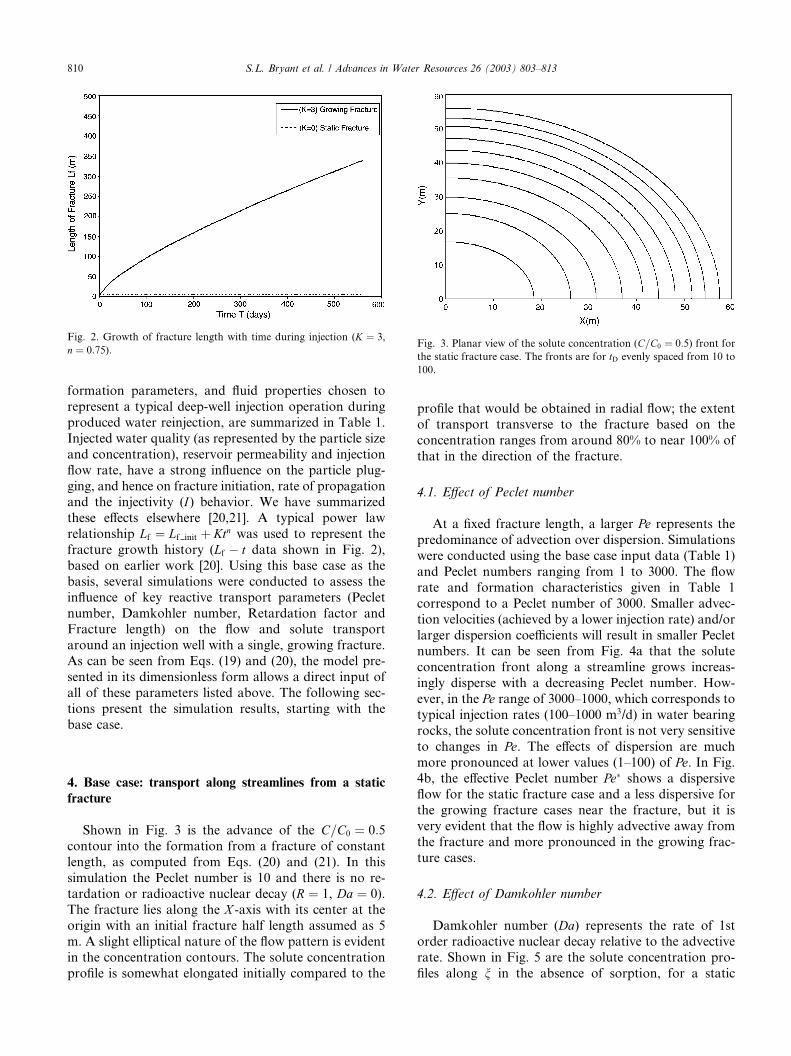
Fig. 2. Growth of fracture length with time during injection (K ¼ 3,

n ¼ 0:75).Fig. 3. Planar view of the solute concentration (C=C0 ¼ 0:5) front for

the static fracture case. The fronts are for tD evenly spaced from 10 to

100.


formation parameters, and fluid properties chosen to

represent a typical deep-well injection operation during

produced water reinjection, are summarized in Table 1.

Injected water quality (as represented by the particle size

and concentration), reservoir permeability and injection

flow rate, have a strong influence on the particle plug-

ging, and hence on fracture initiation, rate of propagationand the injectivity (I) behavior. We have summarized

these effects elsewhere [20,21]. A typical power law

relationship Lf ¼ Lf init þ Ktn was used to represent the

fracture growth history (Lf � t data shown in Fig. 2),

based on earlier work [20]. Using this base case as the

basis, several simulations were conducted to assess the

influence of key reactive transport parameters (Peclet

number, Damkohler number, Retardation factor andFracture length) on the flow and solute transport

around an injection well with a single, growing fracture.

As can be seen from Eqs. (19) and (20), the model pre-

sented in its dimensionless form allows a direct input of

all of these parameters listed above. The following sec-

tions present the simulation results, starting with the

base case.

4. Base case: transport along streamlines from a static

fracture

Shown in Fig. 3 is the advance of the C=C0 ¼ 0:5contour into the formation from a fracture of constant

length, as computed from Eqs. (20) and (21). In this

simulation the Peclet number is 10 and there is no re-tardation or radioactive nuclear decay (R ¼ 1, Da ¼ 0).

The fracture lies along the X -axis with its center at the

origin with an initial fracture half length assumed as 5

m. A slight elliptical nature of the flow pattern is evident

in the concentration contours. The solute concentration

profile is somewhat elongated initially compared to the

profile that would be obtained in radial flow; the extentof transport transverse to the fracture based on the

concentration ranges from around 80% to near 100% of

that in the direction of the fracture.

4.1. Effect of Peclet number

At a fixed fracture length, a larger Pe represents the

predominance of advection over dispersion. Simulations

were conducted using the base case input data (Table 1)

and Peclet numbers ranging from 1 to 3000. The flow

rate and formation characteristics given in Table 1

correspond to a Peclet number of 3000. Smaller advec-

tion velocities (achieved by a lower injection rate) and/or

larger dispersion coefficients will result in smaller Pecletnumbers. It can be seen from Fig. 4a that the solute

concentration front along a streamline grows increas-

ingly disperse with a decreasing Peclet number. How-

ever, in the Pe range of 3000–1000, which corresponds totypical injection rates (100–1000 m3/d) in water bearing

rocks, the solute concentration front is not very sensitive

to changes in Pe. The effects of dispersion are much

more pronounced at lower values (1–100) of Pe. In Fig.4b, the effective Peclet number Pe� shows a dispersive

flow for the static fracture case and a less dispersive for

the growing fracture cases near the fracture, but it is

very evident that the flow is highly advective away from

the fracture and more pronounced in the growing frac-

ture cases.

4.2. Effect of Damkohler number

Damkohler number (Da) represents the rate of 1st

order radioactive nuclear decay relative to the advective

rate. Shown in Fig. 5 are the solute concentration pro-

files along n in the absence of sorption, for a static

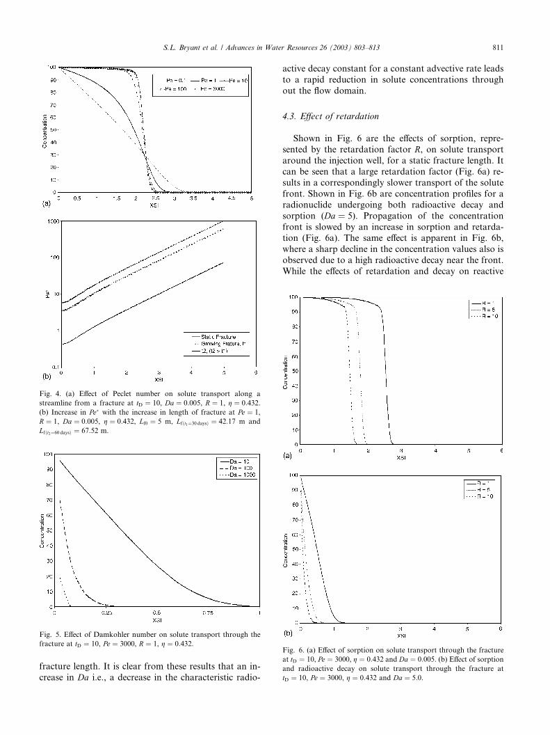
Fig. 5. Effect of Damkohler number on solute transport through the

fracture at tD ¼ 10, Pe ¼ 3000, R ¼ 1, g ¼ 0:432.Fig. 6. (a) Effect of sorption on solute transport through the fracture

at tD ¼ 10, Pe ¼ 3000, g ¼ 0:432 and Da ¼ 0:005. (b) Effect of sorption

and radioactive decay on solute transport through the fracture at

tD ¼ 10, Pe ¼ 3000, g ¼ 0:432 and Da ¼ 5:0.

Fig. 4. (a) Effect of Peclet number on solute transport along a

streamline from a fracture at tD ¼ 10, Da ¼ 0:005, R ¼ 1, g ¼ 0:432.

(b) Increase in Pe� with the increase in length of fracture at Pe ¼ 1,

R ¼ 1, Da ¼ 0:005, g ¼ 0:432, Lf0 ¼ 5 m, Lfðt1¼30 daysÞ ¼ 42:17 m and

Lfðt2¼60 daysÞ ¼ 67:52 m.


fracture length. It is clear from these results that an in-

crease in Da i.e., a decrease in the characteristic radio-

active decay constant for a constant advective rate leads

to a rapid reduction in solute concentrations through

out the flow domain.

4.3. Effect of retardation

Shown in Fig. 6 are the effects of sorption, repre-sented by the retardation factor R, on solute transport

around the injection well, for a static fracture length. It

can be seen that a large retardation factor (Fig. 6a) re-

sults in a correspondingly slower transport of the solute

front. Shown in Fig. 6b are concentration profiles for a

radionuclide undergoing both radioactive decay and

sorption (Da ¼ 5). Propagation of the concentration

front is slowed by an increase in sorption and retarda-tion (Fig. 6a). The same effect is apparent in Fig. 6b,

where a sharp decline in the concentration values also is

observed due to a high radioactive decay near the front.

While the effects of retardation and decay on reactive


transport along Cartesian co-ordinates are well known,

results such as shown in Fig. 6, which demonstrate the

same in an elliptical flow field along n are rare. It shouldbe noted that the distance along a streamline grows

exponentially with n. Thus one should see a difference inthe effects of retardation and Damkohler number when

plotted along the streamline distances, though qualita-

tively they have a similar effect.

4.4. Effect of fracture length: growing fracture case

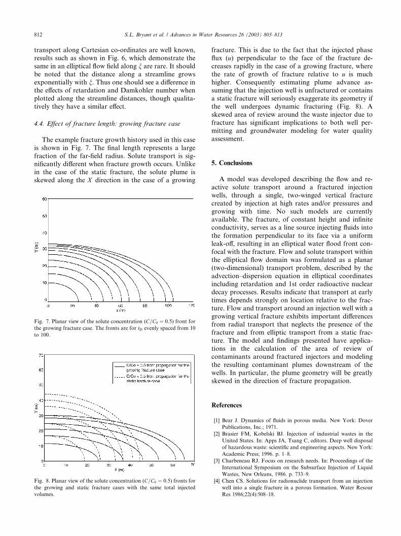
The example fracture growth history used in this case

is shown in Fig. 7. The final length represents a large

fraction of the far-field radius. Solute transport is sig-nificantly different when fracture growth occurs. Unlike

in the case of the static fracture, the solute plume is

skewed along the X direction in the case of a growing

Fig. 7. Planar view of the solute concentration (C=C0 ¼ 0:5) front for

the growing fracture case. The fronts are for tD evenly spaced from 10

to 100.

Fig. 8. Planar view of the solute concentration (C=C0 ¼ 0:5) fronts for

the growing and static fracture cases with the same total injected

volumes.

fracture. This is due to the fact that the injected phase

flux (u) perpendicular to the face of the fracture de-

creases rapidly in the case of a growing fracture, where

the rate of growth of fracture relative to u is much

higher. Consequently estimating plume advance as-suming that the injection well is unfractured or contains

a static fracture will seriously exaggerate its geometry if

the well undergoes dynamic fracturing (Fig. 8). A

skewed area of review around the waste injector due to

fracture has significant implications to both well per-

mitting and groundwater modeling for water quality

assessment.

5. Conclusions

A model was developed describing the flow and re-

active solute transport around a fractured injection

wells, through a single, two-winged vertical fracture

created by injection at high rates and/or pressures and

growing with time. No such models are currentlyavailable. The fracture, of constant height and infinite

conductivity, serves as a line source injecting fluids into

the formation perpendicular to its face via a uniform

leak-off, resulting in an elliptical water flood front con-

focal with the fracture. Flow and solute transport within

the elliptical flow domain was formulated as a planar

(two-dimensional) transport problem, described by the

advection–dispersion equation in elliptical coordinatesincluding retardation and 1st order radioactive nuclear

decay processes. Results indicate that transport at early

times depends strongly on location relative to the frac-

ture. Flow and transport around an injection well with a

growing vertical fracture exhibits important differences

from radial transport that neglects the presence of the

fracture and from elliptic transport from a static frac-

ture. The model and findings presented have applica-tions in the calculation of the area of review of

contaminants around fractured injectors and modeling

the resulting contaminant plumes downstream of the

wells. In particular, the plume geometry will be greatly

skewed in the direction of fracture propagation.

References

[1] Bear J. Dynamics of fluids in porous media. New York: Dover

Publications, Inc.; 1971.

[2] Brasier FM, Kobelski BJ. Injection of industrial wastes in the

United States. In: Apps JA, Tsang C, editors. Deep well disposal

of hazardous waste: scientific and engineering aspects. New York:

Academic Press; 1996. p. 1–8.

[3] Charbeneau RJ. Focus on research needs. In: Proceedings of the

International Symposium on the Subsurface Injection of Liquid

Wastes, New Orleans, 1986. p. 733–9.

[4] Chen CS. Solutions for radionuclide transport from an injection

well into a single fracture in a porous formation. Water Resour

Res 1986;22(4):508–18.


[5] Chen CS, Yates SR. Approximate and analytical solutions for

solute transport from an injection well into a single fracture.

Ground Water 1989;27(1):77–86.

[6] Donaldson EC, Rezaei AA. Analysis of the migration pattern of

injected wastes. In: Proceedings of the International Symposium

on the Subsurface Injection of Liquid Wastes, New Orleans, 1986.

p. 464–84.

[7] EPA/625/6-89/025a. Assessing the geochemical fate of deep-well

injected hazardous waste: a reference guide. R.S. Kerr Environ-

mental Research laboratory, Ada, OK, 1990.

[8] Feenstra S, Cherry JA, Sudicky EA, Haq Z. Matrix diffusion

effects on contaminant migration from an injection well in

fractured sandstone. Ground water 1984;22(3):307–16.

[9] Grisak GE, Pickns JF. An analytical solution for solute transport

through fractured media with matrix diffusion. J Hydrol 1981;

52:47–57.

[10] Grisak GE, Pickens JF. Solute transport through fractured media,

1. The effect of matrix diffusion. Water Resour Res 1980;16(4):

725–31.

[11] Moreno L, Rasmuson A. Contaminant transport through a

fractured porous rock: impact of the inlet boundary condition on

the concentration profile in the rock matrix. Water Resour Res

1986;22(12):1728–30.

[12] Moreno L, Neretnieks I, Eriksen T. Analysis of some laboratory

runs in natural fissures. Water Resour Res 1985;21(7):951–8.

[13] Muskat M. The flow of homogeneous fluids through porous

media. Ann Arbor, MI: J.W. Edwards, Inc.; 1946.

[14] Narasimhan TN, Witherspoon PA, Edwards AF. Numerical

model for saturated–unsaturated flow in deformable porous

media, 3, the algorithm. Water Resour Res 1978;14(2):255–61.

[15] Perkins TK, Gonzalez JA. Changes in earth stresses around a

wellbore caused by radially symmetrical pressure and temperature

gradients. SPE J 1984;(April):129–40.

[16] Perkins TK, Gonzalez JA. The effect of thermoelastic stresses on

injection well fracturing. SPE J 1985;(February):78–88.

[17] Rasmuson A, Neretnieks I. Migration of radionuclides in fissured

rock: the influence of micropore diffusion and longitudinal

dispersion. J Geophys Res 1981;86(B5):3749–58.

[18] Rowe RK, Booker JR. Contaminant migration through fractured

till into an underlying aquifer. Can Geotech J 1990;27(4):484–95.

[19] Sahimi M. Flow and transport in porous media and fractured

rock. VCH, NY: Weinheim; 1995. p. 482.

[20] Saripalli KP, Gadde B, Bryant SL, Sharma MM. Modeling the

role of fracture face and formation plugging in injection well

fracturing and injectivity decline. SPE Paper# 52731 presented at

the 1999 SPE/EPA Exploration and Production Conference,

Austin, TX, 1999.

[21] Saripalli KP, Sharma MM, Bryant SL. Modeling injection well

performance during deep-well injection of liquid wastes. J Hydrol

2000;227:41–55.

[22] Schechter RS. Oil well stimulaton. Englewood Cliffs, NJ: Prentice

Hall; 1985. p. 203–7.

[23] Sudicky EA, Frind EO. Contaminant transport in fractured

porous media: analytical solution for a system o parallel fractures.

Water Resour Res 1982;18(6):1634–42.

[24] Stow SH, Johnson KS. Environmental impacts associated with

deep-well disposal. In: LaMoreaux PE, Vrba J, editors. Hydrog-

eology and management of hazardous waste by deep-well

disposal. Hannover, Germany: International Association of

Hydrogeologists; 1990.

[25] Tang DH, Frind EO, Sudicky EA. Contaminant transport in

fractured porous media: analytical solution for a single fracture.

Water Resour Res 1983;19(6):1489–500.

[26] Wennberg E, Morgenthaler L, Sharma MM. Injectivity decline in

water injection wells: an offshore Gulf of Mexico case study.

Europ Form Dam Symp, The Hauge, 1997.

Documents

Flow and solute transport around injection wells through a single, growing fracture