The Output and Welfare Effects of Fiscal Shocks over

the Business Cycle∗

Eric Sims

University of Notre Dame

NBER, and ifo

Jonathan Wolff

University of Notre Dame

November 20, 2013

Abstract

How does the magnitude of the output response to a change in government spending vary

over the business cycle? What are the welfare effects of fiscal shocks? This paper studies the

state-dependence of the output and welfare effects of shocks to government purchases in a DSGE

model with real and nominal frictions and a rich fiscal financing structure. Both the output

multiplier (the change in output for a one dollar change in government spending) and the welfare

multiplier (the consumption equivalent change in welfare for the same change in spending) move

significantly across states, though movements in the welfare multiplier are quantitatively much

larger than for the output multiplier. The output multiplier is high in bad states of the world

resulting from negative “supply” shocks and low when bad states result from “demand” shocks.

The welfare multiplier displays the opposite pattern – it tends to be high in demand-driven

recessions and low in supply-driven downturns. In an historical simulation based on estimation

of the model parameters, the output multiplier is found to be countercyclical and strongly

negatively correlated with the welfare multiplier.

JEL Codes: E30, E60, E62

Keywords: fiscal policy, government spending shocks, business cycle, welfare

∗We are grateful to Rudi Bachmann, Bob Flood, Tim Fuerst, Jeff Thurk, and seminar participants at NotreDame, the University of Texas at Austin, and the Fall 2013 Midwest Macro Meetings for several comments whichhave substantially improved the paper.

1 Introduction

The recent “Great Recession” and period of near-zero interest rates have led to renewed interest in

fiscal stimulus as a tool to fight recessions. There nevertheless seems to be a lack of consensus con-

cerning some fundamental questions. How large are fiscal output multipliers? Do fiscal multipliers

vary in magnitude over the business cycle? What are the welfare implications of fiscal stimulus?

This paper seeks to address each of the above questions, with particular interest in the wel-

fare implications of fiscal stimulus. To do so, we employ a class of dynamic, stochastic, general

equilibrium (DSGE) models popular among central banks and academic economists. These models

have a real business cycle “backbone” in the sense of optimizing agents and market-clearing, but

feature monopolistic competition, price and/or wage rigidity, as well as other real and nominal

frictions. We focus on non-productive government purchases, from which households receive some

utility flow. We follow the standard definition of the fiscal output multiplier – the change in output

for a one dollar change in government purchases. We define the fiscal welfare multiplier as the one-

period consumption equivalent change in welfare for a one dollar change in government purchases.

In contrast to most of the literature studying fiscal policy within the context of DSGE models,

we solve these models using a second order approximation to the equilibrium conditions. Unlike a

linear approximation, the effects of shocks are state-dependent in a second order approximation.

This state-dependence allows us to study interesting questions concerning how fiscal output and

welfare multipliers vary over the business cycle, and, in turn, how they relate to one another.

We begin by studying a relatively simple sticky price New Keynesian model without capital.

The model features households who consume, supply labor, and save through government bonds.

In addition, the model features monopolistically competitive firms that produce and set prices, and

a government that sets spending exogenously. The government is presumed to have a rich array of

financing resources. They can raise revenue via some combination of lump sum and distortionary

taxation and have access to one period risk free bonds. The government also sets interest rates

according to a conventional Taylor rule. In addition to a government spending shock, the model

also features a productivity shock, which functions as a “supply” shock in that it moves prices and

output in opposite directions, and a preference shock, which acts as a “demand” shock in leading

output and prices to move in the same direction.

Before turning to quantitative analysis of the model, we first develop some intuition for how

government spending shocks should impact welfare at different points in the state space.1 In

particular, we analytically decompose the effect of a change in government spending on flow utility

into three separate terms, which we call the “inefficiency”, the “RBC” (standing for “Real Business

Cycle”), and the “price dispersion” components. The “inefficiency” term is equal to the the output

1Given that households receive utility from government purchases in the model, it is impossible to quantify themagnitude, or even the sign, of “the” fiscal welfare multiplier without making restrictive assumptions. If governmentspending is inefficiently low, then temporary but persistent increases in spending will be welfare-improving. Theconverse will be true when government spending is inefficiently high. Given that we do not know the parametersmapping government spending into utility, there is no straightforward way to determine whether government spendingis too high or too low from a welfare perspective. For this reason, we focus not on the sign or magnitude of “the”fiscal welfare multiplier, but rather on how it changes as the state of the economy varies.

1

multiplier times a term proportional to the “labor wedge,” which measures the extent to which the

marginal rate of substitution between consumption and leisure differs from the marginal product

of labor. Because of monopolistic competition, the labor wedge will be positive in steady state

absent a labor subsidy. Because of staggered price-setting, it will endogenously move across states

in the direction opposite inflation – e.g. average markups will be low in inflationary states, and

hence the overall distortion will be small. Holding the output multiplier fixed, we therefore expect

the inefficiency term to be relatively small during supply-driven recessions (when inflation is high),

and large during deflationary demand-driven recessions.

The second term in the approximation to household utility, or what we call the “RBC” com-

ponent, measures the difference between the marginal utilities of public and private consumption.

We call it the “RBC” effect because, in an undistorted flexible price model, a social planner would

equate these two marginal utilities. The “RBC” term will tend to be negative in states where

the marginal utility of private consumption is high. To the extent to which the marginal utility

of consumption is high during recessions, the “RBC” component will work to make the welfare

multiplier procylical. Finally, the “price dispersion” term measures the welfare costs arising from

staggered pricing. In the region of a zero inflation steady state, this term will be zero. Away from

the steady state, this will not be the case. Positive government spending shocks raise inflation.

How higher inflation affects price dispersion depends on whether inflation is initially high or low.

In an inflationary state, an increase in inflation raises price dispersion; in a deflationary state, more

inflation reduces price dispersion. In a supply-driven recession, where inflation is high, a positive

shock to government spending results in higher price dispersion, which works to lower welfare. The

converse is true in a demand-drive recession.

With no capital in the model, the output multiplier is equal to one plus the “consumption

multiplier.” Whether the output multiplier is greater or less than unity depends on the sign of

the consumption response to a spending shock, which could be positive or negative depending on

preferences. Gaining intuition for how the output multiplier ought to vary across the state space

is not as straightforward as in the case of the welfare multiplier. One might think that the output

multiplier would be larger in states where the marginal utility of consumption is high – in these

states, consumption is relatively dear, so consumption ought to increase by more (or decrease by

less) than when marginal utility is low. To the extent to which recessions are times of high marginal

utility, this channel would make the output multiplier countercyclical. On the other hand, because

of staggered pricing, the effective level of distortion in the economy is shock dependent: distortions

will be relatively low in inflationary states and high in deflationary states. One might reason that

output would be more responsive to spending shocks in less distorted states. This would make the

output multiplier larger in supply-driven recessions, but low in demand-driven downturns.

In quantitative simulations of the model, based on the preference specification and parameter-

ization in Christiano, Eichenbaum, and Rebelo (2011), we find that the output multiplier is high

in bad states caused by negative supply shocks, and low in recessions driven by demand shocks.

This means that there is no clear unconditional cyclicality to the output multiplier – its corre-

lation with the level of output is shock-dependent. Consistent with the analytical intuition from

2

the approximation to utility, the welfare multiplier is high in demand-driven recessions and low in

supply-driven downturns. This means that the output and welfare multipliers are negatively corre-

lated with one another – in states in which the output multiplier is high, the welfare multiplier is

low, and vice-versa. Output multipliers are significantly higher under an interest rate peg, such as

would characterize the recent zero lower bound period. Through the “inefficiency” term, which is

equal to the product of the labor wedge and the output multiplier, this also works to make welfare

multipliers larger in all states relative to when the central bank follows a standard Taylor rule. The

state-dependence owing to the “RBC” and “dispersion” terms remains, so that given a policy rule

of pegging the interest rate, the welfare multiplier stills tends to be smaller in recessions caused by

supply shocks and higher in bad times owing to negative demand shocks.

We then extend our analysis to a more realistic version of the model similar to the “medium

scale” DSGE models popularized by Christiano, Eichenbaum, and Evans (2005) and Smets and

Wouters (2003, 2007). In addition to a preference and a productivity shock, the medium scale

model includes a shock to the marginal efficiency of investment and a monetary policy shock, as

well as endogenous capital accumulation, variable capital utilization, nominal wage rigidity, and

a couple of other real frictions. Though the model is substantially more complicated, the basic

intuition for the state-dependence of the welfare multipliers is the same – the welfare effects of

a spending shock will tend to be large in relatively undistorted, inflationary states, and low in

distorted, deflationary states.

To conduct quantitative analysis, we first estimate several parameters of the medium scale

model via Bayesian maximum likelihood using observed data from the US for the period 1985-

2012. Evaluated in the non-stochastic steady state, the output multiplier is estimated to be about

1.2. Under baseline financing assumptions, the welfare multiplier evaluated in steady state is 3.37

units of one period’s consumption. As in the simpler model, the output multiplier is higher in

bad states of the world caused by “supply” shocks and lower in bad states owing to “demand.”

Consistent with our analytical intuition from the simpler model without capital, the reverse is true

for the welfare multiplier – it tends to be low during supply-drive recessions and high when output

is low due to deficient demand. Output multipliers can be significantly higher (in excess of 2) under

an interest rate peg. Owing largely to the positive “inefficiency” effect, the welfare multiplier tends

to be larger under an interest rate peg than not, but still moves in the same ways across the state

space.

We then turn to an historical simulation. Using the estimated parameter values and observed

data, we use the Kalman smoother to construct restrospective smoothed estimates of the unobserved

state variables in the model. The smoothed states are then used to construct output and welfare

multipliers at each point in time. In a simulation ignoring the zero lower bound, the output

multiplier ranges from a minimum of about 1.05 (at the height of the “dot-com bubble”) to a

maximum of 1.5 during the most recent recession. The welfare multiplier ranges from 1.10 to

4.81. The welfare multiplier is about 9 times more volatile than the output multiplier, as measured

by the standard deviations of each series. The estimated output and welfare multipliers have a

correlation coefficient of -0.90. The output multiplier is unconditionally countercyclical (correlation

3

with HP detrended output of -0.40), while the welfare multiplier is procyclical (correlation with

detrended output of 0.41). In a simulation taking the zero lower bound into account, the output

multiplier in the period 2009-2012 is estimated to be substantially higher, with a mean value of

2.0 during that period and a maximum value of 2.76. The welfare multiplier is also higher on

average, but continues to co-move negatively with the output multiplier (correlation during the

2009-2012 subsample of -0.42). The output multiplier during the zero lower bound episode is even

more strongly countercyclical than over the rest of the sample, while the welfare multiplier remains

mildly procylical.

Our paper is related to a growing literature on fiscal policy multipliers. There is a large em-

pirical literature that seeks to estimate fiscal output multipliers using reduced form techniques.

Using orthogonality restrictions in estimated vector auto-regressions (VARs), Blanchard and Per-

otti (2002) identify shocks by “ordering” government spending first in a recursive identification,

and report estimates of spending multipliers between 0.9 and 1.2. Mountford and Uhlig (2009) use

sign restrictions in a VAR and find a multiplier of about 0.6. Ramey (2011) uses narrative evidence

to construct a time series of government spending “news,” and reports multipliers in the range of

0.6-1.2. This range aligns well with a number of papers that make use of military spending as an

instrument for government spending shocks in a univariate regression framework (see, e.g. Barro,

1981; Hall, 1986 and 2009; Barro and Redlick, 2009; Ramey and Shaprio, 1988; and Eichenbaum

and Fisher, 2005). The bulk of this empirical literature suggests that spending multipliers are

around 1. Because these estimates are based on full sample averages, they cannot speak to any

form of state-dependence, and given non-observability of utility, these empirical papers cannot say

anything about welfare.

There is also a limited but growing literature that seeks to estimate state-dependent multi-

pliers using econometric techniques. A drawback of this approach is that there are limited time

series observations, particularly during periods of economic slack. Auerbach and Gorodnichenko

(2012) estimate a regime-switching VAR model and find that output multipliers are highly coun-

tercylical and as high as 3 during recessions and as low as 0 during expansions. Bachmann and

Sims (2012) and Mittnik and Semmler (2012) use similar methods and reach similar conclusions.

Owyang, Ramey, and Zubairy (2013) use newly constructed historical data and Jorda’s (2005) “lo-

cal projection” technique to study state-dependent multipliers. For the US they find no evidence

of countercyclical output multipliers, while for Canada they do. All of these papers measure the

state of the economy solely by the level of output relative to a trend. Our quantitative analysis

suggests that this may be a mistake: the magnitude of the output multiplier seems to depend on

the kind of shock driving output to a low or high level, not the level of output per se.

Another strand of the literature, closer to the current paper, looks at the magnitude of fiscal

output multipliers within the context of DSGE models. Baxter and King (1993) is an early contri-

bution. Monacelli and Perotti (2008) point out that multipliers can be greater or less than unity

depending on the exact preference specification. Zubairy (2013) estimates a medium-scale DSGE

model similar to the one presented in the current paper and finds the output multiplier to be about

1.1. Coenen, et al (2012) calculate fiscal multipliers in seven popular DSGE models, and conclude

4

that fiscal multipliers can be sizable. Cogan, Cwik, Taylor and Wieland (2010) draw a different

conclusion on the basis of a similar model. Drautzberg and Uhlig (2011) also find relatively small

multipliers in similar models. Leeper, Traum, and Walker (2011) use Bayesian prior predictive

analysis to try to provide plausible bounds on multipliers. As noted by Parker (2011), almost all

of the DSGE work, including that cited here, is based on linear approximations, which necessarily

cannot address the state-dependence of multipliers.

A third strand of the literature looks at output multipliers and their interaction with the

stance of monetary policy. In particular, there is a growing consensus that output multipliers can

be substantially larger than normal under “passive” monetary policy regimes, such as the recent

zero lower bound period. Early contributions in this regard are Christiano (2004) and Eggertson

(2004). Woodford (2011) conducts some analytical exercises in the context of a conventional New

Keynesian model without capital to study the fiscal output multiplier, both inside and outside of a

zero lower bound episode. Most recently, Christiano, Eichenbaum, and Rebelo (2011) analyze the

consequences of the zero lower bound for government spending multipliers in DSGE models similar

to the ones in the current paper, and find that multipliers can be very large, in excess of 2. Though

Christiano, Eichenbaum, and Rebelo (2011) are mostly focused on the output multiplier, they do

briefly examine welfare, and find that it is optimal to substantially increase government spending

at the zero lower bound. This conclusion accords with our finding that welfare multipliers are

typically larger at the zero lower bound because of a positive “inefficiency” effect. As their analysis

is based on linearization, they do not discuss other state-dependence of government spending shocks

on welfare. Nakata (2013) reaches a similar conclusion that it is optimal to increase government

spending when the zero lower bound binds. His is one of the only papers of which we are aware

which makes of non-linear solution techniques in the context of studying fiscal multipliers, though

he does not look at the kind of state-dependence that we do.

The contribution of our paper is to bring together some of these somewhat disparate literatures.

Even though there is some (contested) reduced-form empirical evidence about state-dependent

output multipliers, there has been little or no attempt to connect this evidence with micro-founded

models. Even though the tools for solving DSGE models through higher order approximations are

widely available, we are aware of no other paper which looks at the dependence of output multipliers

on the state of the economy in a DSGE context (other than the zero lower bound binding). In a

relatively standard medium scale model, we find that the output multiplier varies substantially –

from about 1 to 1.5 ignoring the zero lower bound, and from 1.5 to 2.75 when the interest rate is

pegged. Future work connecting this state-dependence from a standard DSGE model with some

of the reduced form evidence seems worthwhile. We are also one of only a few papers which look

at the welfare consequences of fiscal shocks, and the only, of which we are aware, that looks at

how the welfare effects of fiscal shocks are related to the output effects. Indeed, we find that the

welfare and output multipliers in these models are typically negatively correlated. To the extent

to which one wants to use a micro-founded DSGE model for policy analysis, one ought to look at

model-implied welfare effects of spending shocks, not the output effects. Our results suggest that

the output multiplier is likely a poor measure of the welfare effect of a fiscal shock.

5

2 The Basic New Keynesian Model

The first part of this section briefly describes a conventional New Keynesian model, which serves

as our laboratory for investigating the size of the fiscal welfare multiplier and its relation to the

output multiplier. The second part of the section provides some analytical intuition for how the

multipliers ought vary across the state space and with each other.

2.1 The Model

The model is comprised of a household, a continuum of intermediate goods firms, a final good firm

that aggregates the intermediates into a consumption good, and a government. Below we lay out

the decision problems facing each agent and define an equilibrium.

2.1.1 Household

There is a representative household which receives utility from consumption, leisure, and gov-

ernment purchases (which it takes as given); earns income from working; saves through risk-free

government bonds; and pays taxes to the government. It behaves as a price-taker. Its problem is:

maxCt,Nt,Bt

E0

∞∑t=0

βtνtU(Ct, 1−Nt) + Ω(Gt)

s.t.

(1 + τ ct )Ct +BtPt≤ (1− τnt )wtNt + Πt + Tt + (1 + it−1)

Bt−1

Pt

Ct is consumption, Nt is labor supply, and Gt is government purchases. Lt = 1−Nt is leisure.

Both U(·) and Ω(·) are increasing and concave in their arguments. Pt is the nominal price of

goods. We abstract from money. Bt−1 is the nominal quantity of government bonds with which a

household enters a period. it−1 is the interest rate that pays off in period t on bonds held between

t − 1 and t. Πt is redistributed profit from firms and Tt is lump sum taxes, both of which the

household takes as given. τ ct and τnt are consumption and labor income taxes, respectively. wt is

the real wage. νt is a preference shock and β is the discount factor.

First order necessary conditions for a solution to the problem are:

µt =νtUC(Ct, 1−Nt)

1 + τ ct(1)

UL(Ct, 1−Nt)

UC(Ct, 1−Nt)=

1− τnt1 + τ ct

wt (2)

µt = βEtµt+1(1 + it)(1 + πt+1)−1 (3)

Equation (1) defines the tax-adjusted marginal utility of consumption as µt, where µt is the

Lagrange multiplier on the budget constraint. (2) is the labor supply condition and (3) is the Euler

equation for bonds, where πt = PtPt−1− 1. Household welfare can be expressed recursively as:

6

Vt = νtU(Ct, 1−Nt) + Ω(Gt) + βEtVt+1 (4)

The preference shock is assumed to follow a mean zero stationary AR(1) process in the log,

with eν,t drawn from a standard normal distribution and sν the standard deviation of the shock:

ln νt = ρν ln νt−1 + sνeν,t (5)

2.1.2 Final Good Firm

There are a continuum of intermediate good firms, indexed by j ∈ (0, 1). A representative final

good firm aggregates these intermediates into a final good available for consumption using a CES

aggregator, where εp > 1 is the elasticity of substitution among intermediates:

Yt =

(∫ 1

0Yt(j)

εp−1

εp dj

) εpεp−1

(6)

Profit maximization gives rise to a demand curve for each intermediate and the zero profit

condition yields an expression for an aggregate price index:

Yt(j) =

(Pt(j)

Pt

)−εpYt (7)

P1−εpt =

∫ 1

0Pt(j)

1−εpdj (8)

2.1.3 Intermediate Goods Firms

Intermediate goods firms produce output using labor and a common productivity term, At, accord-

ing to a constant returns to scale technology:

Yt(j) = AtNt(j) (9)

Intermediate goods firms all face the same wage. Cost-minimization implies that all have a

common real marginal cost, equal to the ratio of the real wage to productivity:

mct =wtAt

(10)

The productivity variable is assumed to follow a stationary mean zero AR(1) process in the log.

The shock ea,t is drawn from a standard normal distribution with sa the standard deviation of the

shock:

lnAt = ρa lnAt−1 + saea,t (11)

Each firm faces a constant probability, 1−θp, of being able to adjust its price each period. This

probability is independent of when a firm’s price was last adjusted, and is therefore also equal to

7

the fraction of updating firms. The possibility of not being able to update price makes the pricing

problem of updating firms forward-looking. Updating firms discount future profits by the stochastic

discount factor of the household, equal to βs µt+sµt, as well as the probability of being stuck with the

current price, θsp. Non-updating firms can index their price in each period to lagged inflation at

ζp ∈ (0, 1). The pricing problem can be expressed:

maxPt(j)

Et

∞∑s=0

(βθp)s µt+sµt

(s∏

m=1

(1 + πt+m−1)ζp(1−εp)Pt(j)1−εpP

εp−1t+s Yt+s −

s∏m=1

(1 + πt+m−1)−ζpεpPt(j)−εpmct+sP

εpt+sYt+s

)

The first order condition is an optimal reset price that will be the same for all updating firms,

P#t . It can be written recursively, where π#

t =P#t

Pt−1− 1, in terms of only aggregate variables:

1 + π#t

1 + πt=

εpεp − 1

X1,t

X2,t(12)

X1,t = mctµtYt + θpβEt(1 + πt)−ζpεp(1 + πt+1)εpX1,t+1 (13)

X2,t = µtYt + θpβEt(1 + πt)ζp(1−εp)(1 + πt+1)εp−1X2,t+1 (14)

2.1.4 Government

We do not model an explicit Ramsey problem for the government. Rather, we postulate the

existence of simple rules for both monetary and fiscal policy. Monetary policy is set according to a

standard Taylor-type rule in which the interest rate reacts to deviations of inflation from exogenous

target, π∗, and to output growth. i∗ = β−1(1 + π∗) is the steady state nominal interest rate:

it = (1− ρi)i∗ + ρiit−1 + (1− ρi) (φπ(πt − π∗) + φy(lnYt − lnYt−1)) (15)

On the fiscal side, the government budget constraint is:

Gt + it−1Bg,t−1

Pt= τ ct Ct + τnt wtNt + Tt +

Bg,t −Bg,t−1

Pt(16)

Bg,t−1 is the stock of debt with which the government enters period t. Government expenditure

plus interest payments on outstanding debt must equal tax collections plus issuance of new debt.

The tax instruments follow AR(1) processes with a non-negative response to the deviation of

government debt from an exogenous long run target level, B∗g . Some or all of the tax instruments

must react sufficiently to debt so as to satisfy a no-Ponzi condition:

τ ct = (1− ρc)τ c + ρcτct−1 + (1− ρc)γc(Bg,t−1 −B∗g) (17)

τnt = (1− ρn)τn + ρnτnt−1 + (1− ρn)γn(Bg,t−1 −B∗g) (18)

Tt = T ∗ + γT (Bg,t−1 −B∗g) (19)

τ c, τn, and T are the steady state values of the tax rates. Because the exact timing of lump

8

sum taxes is irrelevant, it is without loss of generality to not include an AR(1) term in the process

for lump sum taxes. Government spending is assumed to follow a stationary AR(1) process in the

log, with G∗ the steady state level of spending, and eg,t a shock drawn from a standard normal

distribution and sg the standard deviation of the shock:

lnGt = (1− ρg)G∗ + ρg lnGt−1 + sgeg,t (20)

2.1.5 Market-Clearing and Equilibrium

The definition of equilibrium is standard: given exogenous processes and endogenous states, it is a

set of prices and non-explosive allocations such that all markets clear, household and firm first order

conditions are satisfied, and monetary and fiscal policy rules are obeyed. Labor market-clearing

requires that Nt =

∫ 1

0Nt(j)dj. Bond market-clearing requires that Bt = Bg,t. Any profits are

returned to households lump sum. Combining these conditions gives rise to a standard aggregate

resource constraint:

Yt = Ct +Gt (21)

Under the properties of Calvo (1983) pricing, the evolution of aggregate inflation can be written

without reference to intermediate subscripts:

1 + πt =(

(1− θp)(1 + π#t )1−εp + θp(1 + πt−1)ζp(1−εp)

) 11−εp (22)

The aggregate production function is:

Yt =AtNt

vpt(23)

Where vpt =

∫ 1

0

(Pt(j)

Pt

)−εpdj is a measure of price dispersion which is bound from below by

one. It can be written recursively without reference to intermediate subscripts as:

vpt = (1 + πt)εp(

(1− θp)(1 + π#t )−εp + θp(1 + πt−1)−εpζpvpt−1

)(24)

Equations (1)-(5), (10)-(14), (15)-(20), and (21)-(24) characterize an equilibrium in the vari-

ables:µt, Ct, Nt, Vt, Yt, v

pt , Gt, Tt, Bg,t, τ

ct , τ

nt , At, νt, wt, mct, X1,t, X2,t, πt, π

#t , it

.

2.2 Intuition

Before proceeding to a higher order numerical approximation to the solution of the model, it is

helpful to first try to gain some analytical intuition for how these multipliers will be affected by

the state of the economy.

Household welfare, written recursively in (4), is equal to the present discounted value of flow

utility. To gain intuition for how welfare reacts to changes in Gt, it is easiest to focus on how

9

increases in Gt affect current period utility, without regard to subsequent utility flows. Totally

differentiating flow utility about some point (not necessarily the non-stochastic steady state), re-

arranging terms, and using the aggregate accounting identity (21) and production function (23),

gives rise to the following expression for the fiscal “utility multiplier”:

dUtdGt

=

[dYtdGt

(UC − UL

vp

A

)]︸ ︷︷ ︸

Inefficiency

+

[Ω′(G)− UC

]︸ ︷︷ ︸

RBC

−

[ULN

d ln vptdGt

]︸ ︷︷ ︸Price Dispersion

(25)

In order to improve readability, we have suppressed the dependence of the marginal utilities

on the levels of consumption and leisure. We decompose the derivative into three components, set

off by brackets. We call these three terms the “Inefficiency” effect, the “RBC” or “Real Business

Cycle” effect, and the “Price Dispersion” effect. In an efficient flexible price allocation, a planner

would set UC = ULvp

A and there would be no price dispersion, so that the first and third terms

would drop out, leaving only Ω′(G)−UC , which we therefore label the “Real Business Cycle” effect.

In such a model, the welfare multiplier will only depend on the relative marginal utilities of public

and private consumption. If government spending is set such that Ω′(G) > UC , then increases

in Gt will be welfare-improving and vice-versa. Moving across the state space, the “RBC effect”

will tend to be smaller in periods when the marginal utility of consumption is high, such as in a

recession induced by a sequence of negative supply shocks. In contrast, in a recession resulting from

preference shocks, the “RBC effect” will be larger because the marginal utility of consumption is

low.

In general, the equilibrium of the New Keynesian model is inefficient because of monopoly

power in price-setting and endogenous movements in markups from sticky prices. Unless labor is

appropriately subsidized, UC −UL vp

A , which is proportional to a term sometimes referred to as the

“labor wedge” (Chari, Kehoe, and McGrattan, 2007), will be positive, making the “Inefficiency”

effect positive in the neighborhood of the steady state. In other words, if the allocation of labor in

equilibrium is inefficiently low, then increases in government spending, which raise hours, will have

a positive effect on utility. In bad states of the world caused by negative supply shocks, inflation

will be high and markups will be relatively low, so UC − UL vp

A will be small. Holding the output

multiplier fixed, the welfare effect of an increase in government spending will be lower than normal

in a recession caused by supply shocks. The converse will true in a deflationary demand-driven

recession.

The third term in the utility multiplier is proportional to the effect of a change in government

spending on price dispersion. Since UL > 0, increases in price dispersion will work to lower the

utility multiplier. Increases in government spending raise “demand,” which leads to an increase in

inflation. How an increase in inflation affects price dispersion depends on whether the economy is

initially in an inflationary or deflationary state. In states where inflation is close to zero,d ln vptdGt

≈ 0,

so there is no effect of government spending on price dispersion. In bad states of the world caused

by negative productivity shocks, inflation tends to be high. An increase in inflation when inflation

is already high increases price dispersion, which exerts a negative effect on the utility multiplier.

10

When output is low because of negative demand shocks, in contrast, inflation is low, and increases

in inflation lower price dispersion, which has a positive effect on the utility multiplier.

For a fixed value of the output multiplier, in our model all three of the “Inefficiency,” “RBC,”

and “price dispersion” terms will tend to be low in supply-induced recessions and high in demand-

induced recessions.2 The desirability of counteryclical government spending would thus be depen-

dent on the kind of shock driving output to be low. This conclusion is complicated by the fact that

the “Inefficiency” term is equal to the product of the output multiplier and the labor wedge – if the

output multiplier is high when the “labor wedge” is low, such as in a supply-induced recession, the

overall “Inefficiency” effect could actually be larger than normal. It is not straightforward to sign

the state-dependence of the output multiplier. Since the effect of a spending increase on output is

equal to one plus the “consumption multiplier” (which can be seen by totally differentiating the

resource constraint), one might expect the output multiplier to high when the marginal utility of

consumption is high, since consumption is relatively dear in such states. This would tend to make

the output mutliplier large in supply-driven recessions, and low in a preference-shock induced re-

cession. One might also imagine that the overall level of distortion in the economy could impact the

output multiplier: in states where the economy is relative undistorted (supply-driven recessions), it

may be that labor supply is more elastic, and so the output multiplier is larger, with the converse

true in demand-driven downturns where distortions are large. In any event, to the extent to which

there is state-dependence in the output multiplier, any intuition based on the “inefficiency” term

in the utility approximation is complicated. We therefore defer any definitive conclusions about

the state dependence of the output multiplier, and its correlation with the utility multiplier, to a

quantitative analysis of the model.

2.3 Intuition Under an Interest Rate Peg

Instead of assuming that the interest rate obeys the feedback rule (15), suppose that the central

bank chooses to peg the interest rate at a constant value for a finite (and known) period of time.

That is, it+j = it−1 for j = 0, . . . ,H, where H is the length of the peg. After H periods, the interest

rate is expected to obey the Taylor rule. The zero lower bound is a special case of an interest rate

peg, with it−1 = 0 where the Taylor rule would call for it+j < 0. In our terminology, H would

represent the expected duration of a zero lower bound episode.

As emphasized in Christiano, Eichenbaum, and Rebelo (2011), the output multiplier for a

change in government spending is typically much larger under an interest rate peg than when the

central bank follows a Taylor rule. The intuition for this result is straightforward and based on

the output multiplier. Under a standard Taylor rule, an increase in government spending leads to

higher inflation, but the interest rate reacts by more than the increase in inflation, leading to an

2That the “RBC” effect will be small in a demand-induced recession is conditional on a preference shock tomarginal utility being the source of a demand shock. If demand were low due to contractionary monetary shocks, forexample, UC would low, not high, making the “RBC” term larger than normal in a demand-driven recession. In thesection with the medium-scale model, we quantitatively show that the overall effect of a spending shock on welfareis lower in a bad state caused by monetary policy shocks.

11

increase in the real interest rate. The higher real interest rate works, other things being equal, to

reduce consumption, which keeps dCtdGt

down. When the nominal interest rate is unresponsive to

current conditions, in contrast, this process works in reverse. Higher inflation, rather than leading

to higher real rates, results in lower real rates, which works to simulate consumption and raises

the output multiplier. The longer is the interest rate peg, the more inflationary is a government

spending shock. This leads to even bigger declines in real rates and more stimulative effects on

consumption and hence output. Thus, one should expect the output multiplier to be increasing in

H.

Intuition for the welfare effect of an increase in government spending under an interest rate peg

can again be gleaned from (25). If the economy is distorted, so that UC − UL vp

A > 0, then the

higher output multiplier, dYtdGt

, that obtains under an interest rate peg means that the “inefficiency”

term in (25) is larger than under the Taylor rule. This effect on its own tends to make government

spending increases more attractive from a welfare perspective when the interest rate is pegged.

The “RBC” effect is not directly influenced by an interest rate peg, and will still work to make the

welfare multiplier small in states of the world in which the marginal utility of consumption is high.

As discussed above, government spending increases are inflationary, the moreso the longer is

the duration of the peg. If the economy sits in a state of the world in which inflation is not already

close to zero, this increase in inflation can have a substantial effect on price dispersion. In an

inflationary state, a government spending increase will lead to a large increase in price dispersion

under an interest rate peg, which exerts an even more negative effect on welfare than under the

standard Taylor rule. In contrast, in a deflationary state, an increase in inflation reduces price

dispersion, which has a positive effect on the utility multiplier. Since an interest rate peg works

to exacerbate the inflation response to a spending increase, the peg has the effect of magnifying

the price dispersion effect on welfare – in states of the world where the price dispersion effect is

positive under a Taylor rule, it is even more positive under an interest rate peg; whereas in states

where the price dispersion effect is negative, it is even more negative under a peg.

3 Quantitative Analysis in the Basic Model

In this section we conduct quantitative analysis of the basic New Keynesian model of the pre-

vious section. The quantitative results conform with the intuition discussed above. We begin

by discussing the functional form for the utility function, our parameterization, and our solution

methodology. We then analyze the output and welfare effects of government spending changes

under different fiscal financing regimes which correspond to different levels of distortion in the

economy. Lastly, we extend our quantitative analysis to the case of an interest rate peg.

3.1 Functional Form, Parameterization, and Solution Methodology

We assume that period utility from consumption and leisure takes the following form:

12

U(Ct, 1−Nt) =

(Cγt (1−Nt)

1−γ)1−σ − 1

1− σ, σ > 0, 0 < γ < 1 (26)

This is the functional form used by Christiano, Eichenbaum, and Rebelo (2011). It is consistent

with balanced growth for all permissible values of σ and γ. When σ → 1, the utility function reverts

to the popular log-log form of γ lnCt + (1− γ) ln(1−Nt). When σ > 1, consumption and labor are

complements, so UCN > 0. This means that the marginal utility of consumption is higher when

labor hours are higher. Since government spending increases raise hours, complementarity between

consumption and labor helps to keep consumption from falling too much when Gt increases or even

allows it rise, which means that the multiplier can be greater than one. With the conventional

separable specification of preferences, in contrast, it is difficult to get output multipliers in excess

of unity.

We assume that the function mapping government spending into period utility is logarithmic:

Ω(Gt) = ϕ lnGt, ϕ > 0 (27)

The parameter ϕ governs the extent to which the household derives utility from government pur-

chases.

We follow the parameterization in Christiano, Eichenbaum, and Rebelo (2011). We set σ = 2

and γ = 0.3. The discount factor is set to β = 0.99. We set the Calvo parameter for price-setting

at θp = 0.85. This is high relative to available micro evidence; we will use a more conventional

value of this parameter in the medium scale version of the model in the next section. The elasticity

of substitution among intermediate goods is set to εp = 10, which implies steady state markups

of about 10 percent. We assume no price indexation, so ζp = 0. The parameters of the Taylor

rule are ρi = 0.7, φπ = 1.5, and φy = 0.125. We assume zero trend inflation as a benchmark,

π∗ = 0. We assume that government financing is all lump sum, so γnb = γcb = ρc = ρn = 0. We

set γTb = 0.05 and target a steady state government debt-output ratio of 0.5. With lump sum

financing the magnitude of the debt-output ratio is irrelevant, and the value of γTb is also irrelevant

provided it is large enough to rule out explosive debt paths. Throughout we assume that the steady

state consumption tax is zero, τ c = 0, and is always unresponsive to economic conditions. The

assumption of a zero steady state consumption tax is without loss of generality conditional on the

assumption that γcb = 0; as long as the consumption tax is constant, it plays a role analogous to

the labor income tax in that it only distorts the intratemporal tradeoff between consumption and

leisure. We consider different values of the steady state labor tax, corresponding to differing levels

of steady state inefficiency, in the subsections below.

We take the following approach to picking steady state government consumption. We first set

ϕ = 0.15. Given our other parameterizations, this would imply an optimal steady state level of

government spending amounting to 20 percent of steady state output in an undistorted economy

(e.g. when εp → ∞, or when the steady state labor tax is used to offset the wedge associated

with monopoly power, as described below). This is in line with post-war US data. Our baseline

13

approach to calibrating G∗ is to set it such that Ω′(G∗) = UC(C∗, 1 − N∗). If the steady state

of the economy is distorted, where UC(C∗, 1 −N∗) − UL(C∗, 1 −N∗)vpA > 0, then this level of G∗

does not maximize steady state utility; to maximize steady state utility in a distorted economy

would require Ω′(G∗) < UC(C∗, 1 − N∗). We choose to take this approach, rather than assuming

that steady state government spending always maximizes steady state welfare, because it makes

the “RBC effect” in (25) equal to zero in steady state, which makes it easier to think about welfare

effects of government spending shocks. In the robustness section we analyze how different levels of

steady state government spending affect our analysis.

In terms of the shock processes, we set ρa = ρν = 0.95 and ρg = 0.8. The parameterization

of the persistence of government spending is taken from Christiano, Eichenbaum, and Rebelo

(2011). We set the shock magnitudes where sa = 0.01 and sν = 0.03. In a version of the model

without government spending shocks, this would produce HP filtered output volatility of about 1.1

percent, which is consistent with US data since the mid-1980s, with the productivity and preference

shocks each contributing a roughly equal amount to the total unconditional variance of output. In

computing output and welfare multipliers, we consider one percent shocks to government spending,

with sg = 0.01.

We solve for the policy functions of the model using a second order approximation about the

non-stochastic steady state. Let xt denote a stacked vector of all endogenous variables (states and

controls) observed at time t, expressed in deviations from the non-stochastic steady state. Let st

denote the vector of endogenous and exogenous state variables, also in deviation form. Let et be a

vector of shocks. The general form of the policy function is:

xt =1

2Υ0 + Υ1st−1 + Υ2et +

1

2Υ3 (st−1 ⊗ st−1) +

1

2Υ4 (et ⊗ et) + Υ5 (st−1 ⊗ et) (28)

⊗ is the Kronecker product operator. In a more standard first order approximation all but Υ1

and Υ2 are matrixes of zeros. The details of solving for the Υ coefficient matrixes can be found in

Schmitt-Grohe and Uribe (2004). We use the pruning alogorithm of Kim, Kim, Shaumberg, and

Sims (2003) to ensure the stability of the approximation.

We define the impulse response function as the change in the expected values of the endogenous

variables conditional on the realization of a particular shock equal to one standard deviation in

period t. In a higher order approximation the impulse responses to a shock depend on the initial

value of the state, st−1. Formally, the impulse response function to shock m is IRFm(h) = Etxt+h−Et−1xt+h | em,t = em,t + sm, st−1, where h ≥ 0 is the forecast horizon. Numerically, we compute

the impulse responses as follows. Given an initial value of the state, st−1, we compute two sets of

simulations of the endogenous variables using the same draws of shocks. In one simulation we add

sm to the realization of shock m in period t. We compute the simulations out to a forecast horizon

of H, which we set to 20. We repeat this process T times, average over the realized values of the

endogenous variables at forecast horizons up to H, and take the difference between the average

simulations with and without the extra sm shock in period t. We use a value of T = 150.

The output multiplier is defined as the change in output for a one unit change in government

14

spending. Since the variables in our numerical simulation are expressed in logs, we compute the

multiplier by taking the ratio of the impact response of output to the impact response of gov-

ernment spending (“impact” meaning h = 0), and multiply that by the inverse steady state ratio

of government spending to output to put it in “dollar” terms. In the basic model, the impact

response of output corresponds to the largest response to a spending shock at any forecast horizon.

A natural way to define the welfare multiplier would be to take the ratio of the response of welfare,

Vt, to the response of government spending to to a spending shock on impact. A complication is

that the units of welfare are not directly interpretable. We therefore define the welfare multiplier

as the consumption equivalent change in welfare for a one unit change in government spending. To

compute this, we divide the ratio of the impact response of Vt to the impact response of Gt by the

steady state marginal utility of consumption; e.g. dVtdGt

1µ∗ . This number gives the units of steady

state consumption in the period of the shock that would yield an equivalent change in welfare to the

spending shock. In making this transformation, we multiply by the marginal utility of consumption

evaluated in steady state, even when the impulse responses are evaluated outside of steady state.

This insures that the conversion to consumption units is constant across the state space, and that

the consumption equivalent welfare multiplier is monotonically related to dVtdGt

.

3.2 An Undistorted Steady State

To begin, we assume that the labor income tax rate is set so as to eliminate the steady state

distortion from monopoly power in price-setting. This requires τn = − 1εp−1 < 0. In other words,

to reach the efficient steady state, labor must be subsidized.3 While unrealistic, this assumption

eliminates the “inefficiency” effect in (25), thereby making it a little easier to analyze the welfare

effects of government spending shocks. Though we assume that the steady state labor tax is non-

zero, unless otherwise noted this tax rate is constant, so all other government finance comes through

lump sum taxes.

The first column of Table 1 shows the output and welfare multipliers evaluated in the steady

state. The output multiplier is 1.11. This is close to the baseline multiplier in Christiano, Eichen-

baum, and Rebelo (2011), from whom our parameterization is taken.4 Consumption rises after a

spending shock, and hence the multiplier is greater than one, due to a combination of the com-

plementarity between consumption and labor, the high degree of price rigidity, and the relatively

low level of persistence (ρg = 0.8) of the spending shock. Since the steady state is undistorted,

the “Inefficiency” effect in (25) ought to be zero. By assumption, since we choose steady state

government spending such that Ω′(G∗) = UC(C∗, 1 − N∗), the “RBC” effect will always be zero

in steady state. Finally, since we assume zero trend inflation, the “price dispersion” effect in (25)

ought to also be close to zero in the steady state. Hence, one should expect there to be no reaction

of flow utility to a spending shock starting from an undistorted, zero inflation steady state, and

hence the welfare multiplier ought to be zero. As shown in the table, this is in fact what we find.

3The elimination of this distortion could alternatively be accomplished with a consumption subsidy.4Their baseline output multiplier is 1.05. The slight discrepancy comes from a different parameterization of the

monetary policy rule.

15

The second and third columns show multipliers evaluated in states of the world where output is

low. In the second column, the economy is in a “recession” due to bad productivity shocks, while

in the third column the low level of output results from a sequence of adverse preference shocks.

We take the following approach to coming up with a starting position of the state from which to

calculate these multipliers. We first simulate 1000 periods of data starting from the non-stochastic

steady state using our baseline parameterization, conditional only on one of the non-government

spending shocks at a time (e.g. the standard deviation of the other shock is set to zero). Then we

average over realizations of the state vector when output is in its bottom decile across the 1000

periods, which in both cases corresponds to output being roughly 3-4 percent below steady state.

We then take the average position of the state vector in these periods when output is low as the

starting value of the state in computing impulse responses to a government spending shock. The

output and welfare multipliers are calculated based on these state-dependent impulse responses.

In a bad state of the world generated by productivity shocks, the output multiplier is 1.16,

higher than in steady state. The welfare multiplier, in contrast, is lower than in the steady state.

In particular, the change in welfare from the spending increase in the bad state is equivalent to a

one period reduction in consumption of 0.68. The third column shows multipliers when the bad

state arises from preference shocks. Here the output multiplier is smaller than in steady state –

1.07 vs. 1.11 – and the welfare multiplier is larger, with a consumption equivalent change in welfare

of positive 1.22. The upper row of Figure 1 plots impulse responses of flow utility (left column) and

price dispersion (right column) to a spending shock from three different starting points: (i) steady

state (solid lines), (ii) a recession induced by productivity shocks (dashed lines), and (iii) a recession

induced by preference shocks (dotted lines). The different behavior of the welfare multiplier across

the state space can be understood by focusing on the “RBC” effect and the “price dispersion” effect

from equation (25). In a recession caused by productivity shocks, Ω′(G∗)−UC(C∗, 1−N∗) < 0 and

inflation is high, so the extra inflation caused by the spending shock raises price dispersion. Hence,

both the “RBC” and “Dispersion” effects work to lower welfare conditional on bad productivity

shocks. The reverse is true in a preference shock induced recession, in which both the marginal

utility of consumption and inflation start out low, so that the extra inflation from the shock actually

leads to lower price dispersion.

3.3 A Distorted Steady State

We next drop the assumption that the steady state is undistorted by setting τn = 0. This will

have the effect of making UC − UL vp

A positive. This means that the welfare multiplier ought to be

positive evaluated in the steady state.

The appropriately labeled rows of Table 1 show output and welfare multipliers, in steady state

as well as in bad states generated by either “supply” or “demand” shocks, for the case of τn = 0.

Relative to the steady state, the output multiplier is again larger in a bad state generated by

productivity shocks, and smaller in a bad state generated by demand shocks. Even though the

output multipliers are slightly lower in all states when τn = 0 relative to the undistorted case, the

16

changes in the output multiplier across states are roughly the same. Because of the “inefficiency”

effect in (25) being positive, the welfare multiplier evaluated in steady state is now positive as

predicted, amounting to about 0.50 of one period’s consumption. The welfare multiplier is slightly

negative in a bad state generated by productivity shocks and is positive and higher than in steady

state in a bad state generated by preference shocks.

The bottom panel of Figure 1 shows impulse responses to a spending shock when τn = 0.

Evaluated in a zero inflation steady state (solid line), the spending increase generates a persistent

increase in flow utility, which is the source of the positive welfare multiplier. Starting from a bad

state of the world caused by productivity shocks (dashed lines), price dispersion increases. Flow

utility actually increases immediately on impact, but then turns negative. The present value of the

flow utility responses comes out to be slightly negative, consistent with the numbers from Table

1. Conditional on being in a bad state induced by preference shocks, price dispersion declines and

flow utility increases persistently and by more than when evaluated in the steady state.

Figure 2 shows scatter plots of the output multiplier, the welfare multiplier, and the level of

output (expressed as a deviation from steady state), based on simulations of the model. The upper

row shows simulations conditioning only on productivity shocks (e.g. the standard deviation of

the preference shock is set to 0). Consonant with the results in Table 1, we see that the output

and welfare multipliers are almost perfectly negatively correlated, the output multiplier is coun-

tercyclical (negatively correlated with the deviation of output from steady state), and the welfare

multiplier is procyclical. The middle panel shows scatter plots based on a simulation conditioning

only on preference shocks. The output and welfare multipliers are again almost perfectly negatively

correlated, but the cyclicalities of the output and welfare multipliers flip signs – now the output

multiplier is positively correlated with output while the welfare multiplier co-moves negatively with

output. The final row shows scatter plots when both productivity and preference shocks are used

in generating data from the model. The output and welfare multipliers are inversely related to one

another, with a correlation of -0.81. Finally, it is worth noting that the welfare multiplier appears

to be significantly more volatile than the output multiplier. Since both multipliers are expressed

in terms of one period’s worth of output or consumption, the units are the same and a direct

comparison of volatilities is appropriate. Whereas the output multiplier ranges from about 1-1.2

in these simulations, the welfare multiplier fluctuates between -2 and 2. This suggests that welfare

multiplier is more than an order of magnitude more volatile than the output multiplier.

The rows of Table 1 labeled “τn = 0.25” show multipliers when the steady state labor tax

is 0.25, which corresponds to the economy being highly distorted in steady state. Though this

results in lower output multipliers in all states, the change in the output multiplier across states is

unaffected – the output multiplier is higher in bad states caused by productivity shocks, while it

is lower in bad states resulting from preference shocks. With the greater steady state distortion,

the “inefficiency” effect from (25) is even larger, so the steady state welfare multiplier is even more

positive than when τn = 0. Though qualitatively they move in the same direction, quantitatively

the state-dependence of the welfare multipliers is smaller the more distorted is the steady state. The

change in the welfare multiplier moving from steady state to a bad state conditional on productivity

17

shocks is -0.6860, -0.5580, and -0.3170 for τn = − 1εp−1 , 0, and 0.25, respectively; conditional on

preference shocks, the changes are 1.2090, 1.0020, and 0.5960, respectively. In other words, the

state-dependence of the welfare multiplier seems to be smaller, conditional on either shock, the

more distorted is the steady state.

What is the intuition for the relationship between the steady state distortion and the movement

in the welfare multiplier across the state space? Figure 3 plots steady state utility as a function of

steady state hours, where steady state hours are in turn a function of the steady state labor tax.

Utility is its highest when τn = − 1εp−1 , which corresponds with steady state labor of about 0.35.

The important observation is that utility is concave in N , and flat near the region of the optimal

tax rate. Suppose that the economy is efficient in steady state, but finds itself in a bad state of

the world. Depending on the shock generating the bad state of the world, hours will be either

inefficiently low or high – in other words, UL − UC vp

A will be non-zero. But because utility is flat

in the region of the undistorted steady state, UL − UC vp

A will nevertheless be “small.” Hence, the

“inefficiency” effect in (25) will be small – the change in the welfare multiplier across the state space

will depend mostly on the “RBC” and “dispersion” effects, which are both negative for productivity

shocks and positive for preference shocks. But as the steady state of the economy becomes more

distorted (i.e. as τn rises), UL − UC vp

A gets more positive, which has the effect of working to move

the welfare multiplier in the same direction as the output multiplier. Since the output multiplier

gets larger in bad states caused by productivity shocks, the “inefficiency” effect gets increasingly

positive in such states as the steady state gets more distorted, which partially “undoes” the negative

welfare effects coming from the “RBC” and “dispersion” terms. The reverse is true for preference

shocks, where the output multiplier is smaller in bad states due to demand shocks. If the steady

state is very distorted, the lower output multiplier works to make the welfare multiplier smaller,

partially offsetting the positive influences from the “RBC” and “dispersion” terms.

3.4 An Interest Rate Peg

We next turn to an analysis of the output and welfare multipliers under an interest rate peg. In

particular, we assume that, when government spending changes, the interest rate is held fixed for

H periods.5 The length of the peg, H, is assumed to be known with certainty by the agents in the

economy.6

5To implement this, we augment the monetary policy rule, (15), with both current and anticipated policy shocks:it = (1 − ρi)i∗ + ρiit−1 + (1 − ρi) (φπ(πt − π∗) + φy(lnYt − lnYt−1)) + ei,t + ei,1,t−1 + · · · + ei,H,t−H . In the periodof a government spending shock, say period t, we numerically solve for a sequence of current and anticipated policyshocks, ei,t, , ei,1,t, . . . ei,H,t that will make the interest rate unresponsive, in expectation, to the spending shockfor the current and next H periods. The effect of a government spending shock under a peg is therefore effectively thesum of the “direct” effect of the spending shock along with the effects of the current and anticipated policy shocks.

6Some papers, notably Christiano, Eichenbaum, and Rebelo (2011), assume that the ex-post length of the peg,H, is itself stochastic – each period there is a given probability that the interest rate will remain fixed. While thisleads to a well-defined ex-ante expected length of the peg, there is some probability that the peg will last for a verylong time. Carlstrom, Fuerst, and Paustian (2013) argue that a deterministic exit from the interest rate peg, as weassume here, give rise to more reasonable results than a stochastic peg. In particular, under a deterministic peg, theoutput multiplier for a government spending increase is increasing in the length of the peg, but is bounded from aboveand stays within a plausible range even for very long peg lengths. Under a stochastic exit, in contrast, the output

18

Table 2 shows output and welfare multipliers under interest rate pegs of different length, H.

For the numbers shown in this table, we assume that τn = 0, so that the steady state is distorted.

We generate multipliers in “bad” states conditional on either productivity or preference shocks in

exactly the same way as earlier. Figuer 4 plots values of the multipliers graphically, both for an

undistorted steady state (τn = − 1εp−1) and a distorted steady state (τn = 0). Dashed lines plot

the multipliers for a bad state starting from an undistorted steady state, while dotted lines show

the multipliers evaluated in a bad state when the steady state is distorted. The left column shows

multipliers when the “bad state” is generated with productivity shocks. The right column does the

same when the bad state arises due to preference shocks.

There are several interesting observations. First, output multipliers are monotonically increasing

in the length of the peg in all states. Second, the welfare multiplier evaluated in an undistorted

steady state is zero and unaffected by the length of the peg. The intuition for this is straightforward

– if the steady state is undistorted, then UL − Uc vp

A is zero, and there is no relationship between

the larger output multiplier and the welfare multiplier. Third, when the steady state is distorted,

the welfare multiplier evaluated in the steady state is positive and increasing in the length of the

peg – when UL − UC vp

A is positive, the welfare and output multipliers move in the same direction

holding the “RBC” and “price dispersion” effects constant, so, as the output multiplier increases

with the length of the peg, so too does the welfare multiplier. Fourth, the welfare multipliers

evaluated in “bad” states move in the same direction as without an interest rate peg, and the state-

dependence of the welfare multipliers is larger the longer is the peg. The reason for this is related

to the price dispersion term and the magnitude of the inflation effect of a government spending

shock. Government spending increases raise inflation, the more so the longer is the amount of time

the interest rate is held fixed. If the economy initially sits in an inflationary, supply-driven state,

a larger response of inflation results in an even more negative dispersion effect on welfare. The

converse is true in a deflationary, demand-driven recessionary state.

Finally, the state-dependence of the output multiplier under an interest rate peg flips conditional

on preference shocks. Whereas under the Taylor rule output multipliers in “bad” states owing to

preference shocks were smaller than in steady state, the reverse is true under an interest rate peg.

This is related to the sensitivity of consumption to the real interest rate. Consumption is relatively

more sensitive to the changes in the real rate when the marginal utility of consumption is low under

our preference specification.7 Under a standard Taylor rule, increases in government spending raise

real interest rates. When marginal utility of consumption is low in a bad state of the world,

consumption rises by less (or declines by more) following an increase in G than it does in steady

state, given the heightened sensitivity to interest rates. This works to make the output multiplier

multiplier can grow unboundedly large with the expected duration of the peg. Erceg and Linde (2012) point outan issue that the length of the zero lower bound episode ought to be endogenous – for large enough fiscal stimulus,the expected duration of the zero lower bound will be lower, which works against larger fiscal multipliers under aninterest rate peg. We ignore this issue.

7If one totally differentiates the Euler equation, treating future consumption as constant, one gets: dct = 1UCC

drt.UCC < 0, so consumption is decreasing in the real interest rate. In our model, the third derivative of the utilityfunction is positive, UCCC > 0, meaning there is a precautionary motive. This means that UCC is relatively smaller(in absolute value) when UC is small, so consumption is more sensitive to the real interest rate when UC is small.

19

lower in a bad state of the world caused by preference shocks. Under an interest rate peg, the real

interest rate declines, rather than rises, after an increase in government spending. In a state of the

world in which the marginal utility of consumption is low, this decline in the real interest rate has

a relatively more expansionary effect on consumption, which results in higher output multipliers

in a bad state. For a similar reason, the state-dependence of the output multiplier in a supply-

driven recession is smaller under an interest rate peg than under the Taylor rule, though the output

multipliers remain larger in bad states than in steady state (i.e. there is no sign flip).

3.5 Robustness

The basic conclusions from our quantitative analysis of the model are quite robust. We first

discuss robustness to different parameter values, and then briefly touch on how different fiscal

financing regimes affect our conclusions. We also consider the effects of different specifications

of how government spending impacts utility, as well as the effects of an “automatic stabilizer”

component to government spending. Finally, we consider a third order approximation to examine

sensitivity to our solution technique.

At our baseline parameterization based on Christiano, Eichenbaum, and Rebelo (2011), the

steady state output multiplier is greater than unity. There are three key parameters that lead

to this result: the price stickiness parameter, θp; the parameter governing risk aversion, σ; and

the persistence of government spending shocks, ρg. θp and σ must be sufficiently high, and ρg

sufficiently low, for the output multiplier to be greater than one. σ > 1 is important for this result,

because it introduces complementarity between consumption and labor. σ also has interesting

effects on the magnitude of the output multiplier changes across the state space. When σ is small,

the variations in the marginal utility of consumption across states are smaller (because utility is

closer to linear), which leads to smaller differences in output multipliers across states. The output

multiplier is also increasing in γ, as is the change in the output multiplier across states. At first

pass this seems odd, as the Frisch labor supply elasticity is decreasing in γ. Given non-separability

in preferences, γ also affects the sensitivity of consumption to interest rates, with higher values of γ

resulting in consumption that is less sensitive to real rates. Since government spending shocks raise

real rates, higher γ results in larger increases/smaller declines in consumption, and hence bigger

increases in demand.8 In terms of the stance of monetary policy, output multipliers are larger in

all states when there is a smaller response to inflation, a smaller response to output growth, and

less smoothing in the Taylor rule. The amount of price indexation has little effect on the output

multiplier. Interestingly, output multipliers are larger in all states when there is positive trend

inflation.

The parameters of the model have interesting and intuitive effects on how the welfare multiplier

changes across states. Higher levels of price stickiness, which make output multipliers larger in all

states, tend to exacerbate the changes in welfare multipliers in moving from steady state to a bad

8If prices were flexible, the relationship between γ and the output multiplier would be reversed, with the outputmultiplier decreasing in γ (increasing in the labor supply elasticity). In our baseline parameterization, with θp = 0.85,output is mostly demand determined, so the demand effect of high γ outweighs the labor supply elasticity effect.

20

state. This comes in through the price dispersion effect – the bigger is θp, the more price dispersion

reacts to a spending shock. This exerts a bigger negative effect on the welfare multiplier in a supply-

induced bad state, while it works to have a larger positive effect on welfare in a demand-induced

recession. The state-dependence of the welfare multiplier is decreasing in the value of σ. This is

somewhat interesting in that higher values of σ imply more distaste for non-smooth streams of

consumption. The intuition for why the welfare multiplier is affected by σ in this way relates back

to the way in which σ impacts the output multiplier. When σ is small, the output multiplier varies

less across states. When the steady state is distorted, the “inefficiency” term in (25) is positive,

which works to make the output and welfare multipliers move in the same direction. In bad states

induced by supply shocks, the “RBC” and “dispersion” terms are negative; when σ is low, the

output multiplier increases by less than it would if σ were high, which means that total welfare

falls by more. The reverse is true in the case of a bad state caused by preference shocks. The

state-dependence of the welfare multiplier is increasing in γ. This obtains in spite of the fact that

higher values of γ result in greater state-dependence of the output multiplier, and arises because

higher values of γ imply a greater distaste for uneven streams of consumption and leisure.

Higher values of trend inflation exacerbate the state-dependence of the welfare multiplier. The

effect of an increase in inflation on price dispersion is increasing in the initial state of inflation. In

a supply induced recession, π > π∗, so there is an even bigger negative price dispersion effect on

welfare when trend inflation is positive. In a demand induced recession, π < π∗. The effect of an

increase in inflation on price dispersion is ambiguous, depending not on where current inflation is

relative to trend inflation, but rather where it is relative to zero. If inflation is positive the increase

in inflation from the government spending shock raises price dispersion, exerting a negative effect on

welfare. This tends to make the welfare benefits of a spending shock in a demand-induced recession

smaller. The state-dependence of the welfare multiplier conditional on either demand or supply

shocks is decreasing in the amount of price indexation, ζp. If prices are close to fully indexed, then

the increase in inflation from a government spending shock has smaller effects on price dispersion.

Positive steady state values of the consumption tax work very much like labor income taxes –

they increase the overall level of distortion in the economy, which works to make the “inefficiency”

effect larger. This has the effect of making welfare multipliers larger in all states, and reduces

the change in the welfare multipliers across states. In our baseline simulations, we assume that

all variable government finance comes through lump sum taxes. To that end, we instead suppose

that lump sum taxes are fixed, γT = 0, and that distortionary taxes react to debt, with γn > 0 or

γc > 0. Unless one or both of these are very large, there are not large noticeable affects on output

multipliers, which are measured on impact.9 Naturally, the welfare multipliers tend to be smaller

in all states when distortionary taxes are used for financing, but the overall direction of change

across the states and the magnitudes are similar. We also experimented with different values of

steady state government spending. In our baseline analysis, we pick G∗ so that the “RBC” effect

9Drautzberg and Uhlig (2011) note that “long run” multipliers can be negative under distortionary taxation, andindeed we see some of that in our simulations. The intuition is straightforward – distortionary taxes remain highlong after the spending increase is gone (to pay for the debt accumulated), which acts as a drag on the economy.

21

in (25) is zero. When G∗ is too low relative to this, the “RBC” effect is positive in steady state and

larger in bad states (less negative in the case of productivity-driven recessions, and more positive for

demand-driven slumps). This has the effect of making of making the welfare multipliers larger in all

states, and also leads to smaller changes in the welfare multipliers moving across states. The reverse

pattern obtains when G∗ is set “too high.” The state-dependence of the welfare multiplier in the

case of both supply- and demand-induced recessions is increasing in the persistence of government

spending shocks, ρg.

As in most of the literature, we assume that households receive utility from government spending

in an additively separable way. It may be more realistic to instead model government spending and

private consumption as utility complements. To that end, we consider an alternative specification

of preferences:

U(Ct, 1−Nt, Gt) =

[Gϕt exp

(νt

(Cγt (1−Nt)1−γ)1−σ−1

1−σ

)]1−χ− 1

1− χ(29)

The parameter χ ≥ 0 governs the degree of complementarity between government spending and

private consumption. When χ > 1, government spending and private consumption are utility

substitutes; they are complements when χ < 1. When χ → 1, utility reverts to being additively

separable in the log of government spending, as in our baseline specification. One would imagine

that lower levels of χ, corresponding to more complementarity, would yield larger output multipliers,

since demand will rise more when Gt increases. The approximation to the effect of government

spending changes on flow utility, (25), is fundamentally the same, though one needs to replace

Ω′(G) with UG.

The upper panel of Table 3 shows output and welfare multipliers, evaluated both in steady state

as well as “bad” states caused by either productivity or preference shocks, for different values of χ.

All the parameters are set at their benchmark values, and our procedure for producing “bad” states

is the same as above. We assume that tax rates are all zero, so that the steady state is distorted.

Hence, the first row, with χ = 1, is the same as the τn = 0 row in Table 1. As one might expect,

the output multiplier is higher for lower values of χ in all states of the world – lower values of χ

mean there is a stronger incentive for consumption to increase when government spending increases,

so demand rises more. For productivity shocks, the state-dependence of the output and welfare

multipliers is qualitatively the same as in the benchmark analysis: the output multiplier is higher

in bad states, and the welfare multiplier lower, though the changes in each multiplier across states

are smaller (e.g. the output multiplier only increases by about 0.03 in a bad supply state when

χ = 0.25, as opposed to 0.05 when χ = 1; and the welfare multiplier declines by about 0.45 when

χ = 0.25, as opposed to 0.55 when χ = 1). The effects of complementarity between consumption

and government spending are a little more complicated conditional on preference shocks. For values

of χ suitably close to 1, the output multiplier is lower in bad states caused by preference shocks,

but this flips at very low values of χ. Also, the increase in the welfare multiplier moving to a bad

state conditional on preference shocks is decreasing in χ. The reason for this is straightforward

22

– when consumption and government spending are utility complements, preference shock-driven

recessions are times when the marginal utility of government spending is low, so the gains from

increasing spending are smaller.

In our baseline analysis we assume that government spending is exogenous. We have also

experimented with a specification which allows for an automatic stabilizer component to government

spending. In particular, let actual government spending be the sum of an endogenous component

which reacts to the level of output and an exogenous component, Gt:

lnGt = γyg (lnYt − lnY ∗) + ln Gt (30)

γyg captures the idea that, for a variety of reasons, government spending reacts to the level of

economic activity. The exogenous component of spending, Gt, follows the same AR(1) process as

given in (20).

The lower panel of Table 3 presents output and welfare multipliers for different values of γyg ,

where we assume our benchmark preference specification. We restrict our attention to negative

values, so that the endogenous component of spending is countercyclical. The value of γyg has

little effect on the steady state multipliers. Moving to bad states, more negative values of γyg are

associated with modestly larger output multipliers relative to the case of γyg = 0. Welfare multipliers

in recessionary states, whether driven by supply or demand, are lower for more negative values of

γyg . The reason for this comes from the “RBC” term in (25). If government spending increases

when output is low, then Ω′(Gt) will be low during recessions, which will exert a negative effect on

the welfare multiplier.

Finally, we also have done a robustness check concerning the accuracy of a second order approx-

imation. In computing state-dependent impulse responses away from the point of approximation

(the steady state), it is important that the model not be too non-linear, otherwise these impulse

responses, and the multipliers based on them, could be inaccurate. We have solved the model using

a third order approximation to the equilibrium conditions, and our basic conclusions carry over –

output multipliers vary with the level of output according to shock leading to output being high or

low, and the welfare multiplier tends to move in the opposite direction of the output multiplier.

4 A Medium Scale Model

This section extends the model from Section 2 to include a number of realistic features, among

them capital, sticky wages, habit formation in consumption, and investment adjustment costs. The

model is thus similar to Christiano, Eichenbaum, and Evans (2005) and Smets and Wouters (2007).

4.1 The Model

Below we briefly describe the setup of the model, only highlighting areas where it is different than

the simpler model. The actors in the model are the same as above. The problem of the final goods

firm is identical and so we do not repeat that setup.

23

4.1.1 Household

There is a representative household with preferences over consumption, leisure, and government

spending. We allow for internal habit formation over consumption, with period utility: U(Ct −bCt−1, 1−Nt) + Ω(Gt), where b ∈ (0, 1) is the habit formation parameter. There are two important

modifications to the household budget constraint. First, the household can accumulate physical

capital, Kt, and chooses how intensively to utilize that capital, ut. It then rents capital services,

Kt = utKt, to firms at competitive real rental rate, rkt , potentially subject to a capital income tax

from the government, τkt . Second, the household has some market-power in wage-setting, though

it is subject to nominal frictions similar to that facing firms with regards to price-setting.

Capital obeys the following law of motion:

Kt+1 = Zt

(1− S

(ItIt−1

))It + (1− δ)Kt (31)

S (·) is a convex investment adjustment cost, with the properties that S(1) = S′(1) and S′′(1) > 0.

This specification of the adjustment cost follows Christiano, Eichenbaum, and Evans (2005). Zt

is a shock to the marginal efficiency of investment, as in Justiniano, Primiceri, and Tambalotti

(2010). This shock represents variation in the efficiency of transforming non-consumed output into

productive capital. It obeys a mean zero stationary AR(1) process in the log, with shock, ez,t drawn

from a standard normal distribution with standard deviation sz:

lnZt = ρz lnZt−1 + szez,t (32)

We assume that there is a convex resource cost of capital utilization, ut, given by the function

Γ(·). This function has properties such that Γ(1) = Γ′(1) and Γ′′(1) > 0. The cost of utilization is

proportional to the capital stock, and is expressed in consumption units by dividing by Zt.

Following Schmitt-Grohe and Uribe (2006), labor is supplied to a continuum of labor markets

of measure one, indexed by h ∈ (0, 1). The demand for labor in each market is given by:

Nt(h) =

(wt(h)

wt

)−εwNd,t (33)

wt(h) is the real wage charged in labor market h, wt is the aggregate real wage in the economy

as a whole, and Nd,t is a measure of aggregate labor demand from firms. The parameter εw > 1

is a measure of the elasticity of substitution among different varieties of labor. Each period, the

household can only adjust the wage in a fraction, θw ∈ (0, 1), of the labor markets. The probability

of being able to adjust the wage in a given labor market is independent of when the wage in that

market was last updated. Wages in non-updated markets may be full or partially indexed to lagged

inflation at rate ζw ∈ (0, 1). Total labor supply must satisfy Nt =

∫ 1

0Nt(h)dj. Combining this

with (33), we get:

24

Nt = Nd,t

∫ 1

0

(wt(h)

wt

)−εwdh (34)

The aggregate real wage is an index of wages in each labor market:

w1−εwt =

∫ 1

0wt(h)1−εwdh (35)

This setup differs slightly from models of wage rigidity based on Erceg, Henderson, and Levin

(2000). In those models, households are heterogenous and supply differentiated labor. Staggered

wage-setting plus differentiated labor leads to labor heterogeneity, which would in general spill over

into heterogeneity in consumption and capital accumulation decisions. To avoid this complication, it

is typically assumed that preferences in consumption and leisure are additively separable and that

there exist full state contingent securities which insure households against idiosyncratic income

risk, which means households will have identical consumption and investment, though different

labor supply. The Schmitt-Grohe and Uribe (2006) assumption allows us to consider non-separable

preferences without introducing this level of heterogeneity. The analysis to follow is nevertheless

similar with separable preferences and this alternative assumption on labor markets.

The household budget constraint is given by:

(1 + τ ct )Ct + It + Γ(ut)Kt

Zt+BtPt≤ (1− τkt )rkt utKt + (1− τnt )

∫ 1

0

wt(h)

(wt(h)

wt

)−εwNd,tdh+ (1 + it−1)

Bt−1

Pt+ Πt − Tt

The first order necessary conditions over consumption, utilization, investment, future capital,

labor supply, and bonds are, respectively:

(1 + τ ct )µ1,t = νtUc(Ct − bCt−1, Nt)− βbEtνt+1Uc(Ct+1 − bCt, 1−Nt+1) (36)

(1− τkt )rkt =Γ′(ut)

Zt(37)

1 = qtZt

[1− S

(ItIt−1

)− S′

(ItIt−1

)ItIt−1

]+ βEt

µ1,t+1

µ1,tqt+1Zt+1S

′(It+1

It

)(It+1

It

)2

(38)

qt = βEtµ1,t+1

µ1,t

[(1− τt+1)kRt+1ut+1 −

Γ(ut+1)

Zt+1+ (1− δ)qt+1

](39)

UL(Ct − bCt−1, 1−Nt) = µ3,t (40)

µ1,t = βEtµt+1(1 + it)(1 + πt+1)−1 (41)

Above, µ1,t is the multiplier on the flow budget constraint and µ3,t is the multiplier on (34), the

constraint that the household labor supply meets total demand. qt is the ratio of the multiplier on

the capital accumulation equation to the multiplier on the budget constraint, e.g. qt =µ2,tµ1,t

.

We consider the first order condition over wages separately. As noted above, wages can only

be changed in an exogenously chosen fraction of labor markets, θw ∈ (0, 1). Non-updated wages

25

can be partially or full indexed to lagged inflation by ζw ∈ (0, 1). Reproducing the parts of the

Lagrangian related to the choice of the real wage, the optimal choice of the wage in a particular

market in a period of adjustment must satisfy the first order conditions of:

L = Et

∞∑m=0

(βθw)m

µ1,t+m(1− τnt+m)wt(h)1−εwwεwt+mNd,t+m

(m∏n=1

(1 + πt+m−1)ζw

1 + πt+m

)1−εw

− . . .

µ3,t+mWt(h)−εwW εwt+mNd,t+m

(m∏n=1

(1 + πt+m−1)ζw

1 + πt+m

)−εw]

In this expression, discounting is by the product of β with θw to account for the probability

that a wage chosen in period t will still be in effect in subsequent periods. All updated wages will

be equal to one another, so we can drop h subscripts. We express the optimal updated wage, or

reset wage, as w#t . After some algebraic manipulations, and making use of some of the other first

conditions, the optimality condition over the wage can be written recursively as follows:

w#t =

εwεw − 1

F1,t

F2,t(42)

F1,t = UL(Ct − bCt−1, 1−Nt)Wεwt Nd,t + θwβEt(1 + πt)

−εwζw(1 + πt+1)εwF1,t+1 (43)

F2,t = µt(1− τnt )W εwt Nd,t + θwβEt(1 + πt)

ζw(1−εw)(1 + πt+1)εw−1F2,t+1 (44)

4.1.2 Intermediate Goods Firms

There are again a continuum of intermediate goods firms indexed by j along the unit interval. They

produce output using capital services and labor according to a constant returns to scale production

technology and face a common productivity shock. The productivity process obeys (11). The

production function is:

Yt(j) = AtKt(j)αNd,t(j)

1−α, 0 < α < 1 (45)

These firms are price-takers in input markets. Cost-minimization implies all intermediate goods

firms have the same real marginal cost and hire capital services and labor in the same ratio, which

is equal to the aggregate ratio:

Kt

Nd,t=

α

1− αwt

rkt(46)

mct =w1−αt

(rkt)α

At(1− α)α−1α−α (47)

Given these results from cost-minimization, the price-setting problem of the firm is the same as

described in Section 2.1.3. Hence, the optimal price-setting rule for updating firms is characterized

by (12) - (14).

26

4.1.3 The Government

The behavior of the government is similar to the model without capital. The Taylor rule is given

by (15), government spending obeys a stationary AR(1) as in (20), and consumption, labor, and

lump sum taxes follow (17)-(19).

The government budget constraint needs to be amended to take account of income from capital

taxation. It can be written:

Gt + it−1Bg,tPt

= τ ct Ct + τnt wtNd,t + τkt rkt Kt + Tt +

Bg,t −Bg,t−1

Pt(48)

The capital tax rate obeys the following process, where τk is the exogenous steady state capital

tax rate:

τkt = (1− ρk)τk + ρkτkt−1 + (1− ρk)γkb (Bg,t−1 −Bg) (49)

4.1.4 Market-Clearing and Equilibrium

The definition of equilibrium is the same as for the simpler model without capital. Labor market-

clearing requires that total demand for labor from firms equals the total amount supplied from the

continuum of labor markets; that is,

∫ 1

0Nt(j)dj = Nd,t. Capital market clearing necessitates that

utKt =∫ 1

0 Kt(j)dj. Bond market-clearing requires Bg,t = Bt. Any firm profits are returned lump

sum to the household. Combining these conditions yields the aggregate resource constraint:

Yt = Ct + It +Gt + Γ(ut)Kt

Zt(50)

Capital market clearing requires that:

Kt =

∫ 1

0Kt(j)dj = utKt (51)

Using the fact that all firms hire capital services and labor in the same ratio, as well as the

definition of labor-market clearing, yields the aggregate production function:

Yt =AtK

αt N

1−αd,t

vpt(52)

vpt is the same price dispersion term as in (24). Aggregate inflation obeys (22). The behavior of

the aggregate real wage can be written:

w1−εwt = (1− θw)w#,1−εw

t + θww1−εwt−1 (1 + πt)

εw−1(1 + πt−1)ζw(1−εw) (53)

Aggregate labor supply can be expressed using (34) recursively as:

Nt = Nd,tvwt (54)

27

Where vwt is a measure of wage dispersion:

vwt = (1− θw)

(w#t

wt

)−εw+ θw

(wtwt−1

)εw ((1 + πt−1)ζw

1 + πt

)−εwvwt−1 (55)

Using this, the value function of the representative household can be written without reference

to Nt:

Vt = U(Ct, 1−Nd,tvwt ) + Ω(Gt) + βEtVt+1 (56)

Given initial values of the exogenous variables and endogenous states, equations (5), (11)-(14),

(15), (17)-(19), (22), (24), (31)-(32) (36)-(39), (41)-(44), (46)-(47), (48)-(49), (50)-(53), and (55)-

(56) comprise an equilibrium in the variablesµ1,t, Ct, Nd,t, Vt, Yt, v

pt , Gt, Tt, Bg,t, τ

ct , τ

nt , At, νt, wt,

mct, X1,t, X2,t, πt, π#t , it, w

#t , v

wt , It, ut, Kt, Kt, F1,t, F2,t, τ

kt , r

kt , qt

.

4.2 Intuition

Before proceeding to estimation of the medium scale model and formal quantitative analysis, we

proceed similarly to the model without capital in trying to develop some intuition for the welfare

effects of spending shocks.

After some rearranging, totally differentiating (26) about a point (not necessarily the steady

state), yields:10

dUtdGt

=

[dYtdGt

UC − ULvw vp

(1− α)A(KNd

)α]

︸ ︷︷ ︸Inefficiency

+

[(Ω′(G)− Uc)

]︸ ︷︷ ︸

RBC

−

[ULNdv

w

(d ln vpt1− α

+ d ln vwt

)]︸ ︷︷ ︸

Price/Wage Dispersion

+Ψt

(57)

This approximation to flow utility has a similar interpretation to (25) but with an additional

term, Ψt. We again break the first three terms up into components which we label “Inefficiency,”

“RBC,” and “Dispersion.” The inefficiency effect is equal to the output multiplier times the a

term proportional to the labor wedge, with the only difference relative to (25) that the expression

for the marginal product of labor now depends on the quantities of capital services and labor. If

there is no subsidy to offset the role of monopoly power, this term will be positive in the region of

the steady state. The “RBC” effect is identical to the simpler model. The “Dispersion” term now

depends on both price and wage dispersion. Increases in either work to lower the utility multiplier.

The additional term, Ψt, arises due to the presence of investment and variable capital utilization.

It is given by:

10In taking the total derivative, the current period capital stock is pre-determined and hence does not show up inthis expression.

28

Ψt = −UCdItdGt−

UCΓ′(u)− α

1− αULv

w

(K

Nd

)−1 dutdGt

(58)

As in the simpler model, our basic quantitative approach will be to pick G∗ such that Ω′(G∗) =

UC(C∗, 1 − N∗). Though not necessarily optimal, this makes the “RBC” term equal to 0 in the

steady state. We will also assume that trend inflation is zero, which makes the price/wage dispersion

term equal to zero in the steady state. In general, the steady state of the economy will be distorted,

so that the inefficiency effect will be positive unless labor is appropriately subsidized. It is difficult

to sign Ψt. For most parameterizations of the model, investment will decline when government

spending increases, making the first term of Ψt positive. Utilization will tend to move in the same

direction as hours, and so dutdGt

> 0 for most parameterizations. In the region of a steady state in

which distortionary taxes and inflation are all zero, one can show that the term multiplying dutdGt

will be positive, making the overall sign of Ψt ambiguous.11

The intuition for how the output and welfare multipliers ought to vary across the state space is

essentially the same as in the simpler model without capital. As in the simpler model, the output

multiplier will tend to be high in depressed states of the world driven by supply shocks, and low

when recessions are the result of deflationary demand shocks. There are two additional effects at

play in accounting for movements in the output multiplier across the state space. First, the output

multiplier will tend to be high in states where capital utilization is low – because of convexity

in the utilization adjustment cost function, when utilization is low, it is relatively inexpensive

to ramp up utilization, allowing output to expand by more than in states when utilization is

high. Since utilization is procylical in the model, this effect will tend to make the output multiplier

countercyclical. Second, the lagged level of investment will affect by how much investment responds

to spending shocks through the investment adjustment cost function. For most parameterizations

of the model, investment declines when government spending increases. For a given change in

investment, the percentage change in investment is larger the lower is the initial level of investment.

Since the adjustment cost depends on the percentage change in investment, the absolute decline in

investment after an increase in government spending will be smaller the smaller is the initial level

of investment. With investment falling by less, from the accounting identity output will rise by

more when government spending increases. This effect will also tend to make the output multiplier

countercyclical.

An interest rate peg will have a similar effect on the output and welfare multipliers as in the

simpler model. In particular, under a peg a government spending shock will lower real interest

rates, which will make consumption and investment rise by more (or fall by less) than they do

under a Taylor rule. This works to make the output multiplier larger. The larger output multiplier

contributes to larger welfare multipliers, to the extent to which the steady state is distorted, through

11From (37), Γ′(u) = (1 − τk)rk. Combining this with (46), and assuming that τk = 0, one sees that Γ′(u) =

α1−α

(KNd

)−1

w. This means that the second term in (58) can be written: α1−α

(KNd

)−1

(UCw − ULvw). Evaluating

the steady states of (43) and (44), one sees that Ucw = εwεw−1

UL. As long as εw <∞, Ucw − UL will be positive.

29

the “inefficiency” term. The state-dependence of the welfare multiplier should otherwise be the

same, and if anything ought to be magnified due to a heightened price dispersion term.

5 Estimation and Historical Simulation

This section conducts quantitative analysis of the output and welfare multipliers in the medium

scale model. We begin by estimating some of the parameters of the model to match US data since

the mid-1980s. We then do some quantitative experiments. Finally, we use the estimated model to

back out smoothed values of the historical state vector, which allows us to compute an estimated

time series of output and welfare multipliers.

5.1 Estimation

We assume that period utility function is again given by (26). The investment adjustment cost

function takes the following form: S(·) = κ2

(ItIt−1− 1)2

, where κ ≥ 0. The utilization cost function

takes the form: Γ(·) = Γ0(ut − 1) + Γ12 (ut − 1)2. The parameter Γ1 > 0 is a free parameter. Γ0

is restricted to equal the steady state rental rate on capital, which ensures the normalization that

ut = 1 in steady state.

Our approach is to first calibrate a number of parameters that are closely tied to long run

moments of the data and/or are difficult to estimate. We then estimate the remaining parameters

via Bayesian maximum likelihood. As a benchmark, we assume that all distortionary taxes are

constant, which implies that the method of government finance is irrelevant. We can thus ignore the

parameters governing the tax processes. We assume zero trend inflation. The calibrated parameters

areβ, α, δ, εp, εw, ϕ, Γ1

. We set β = 0.99 and α = 1/3. The elasticity of substitution among

goods and labor are set to εp = εw = 10. We set δ = 0.025. Together, this calibration implies a

steady state investment-output ratio of 21 percent. We again set ϕ = 0.15, and pick G∗ such that

Ω′(G∗) = UC . This implies a steady state government spending-output ratio of 13.5 percent, which

is slightly lower than in the data. Finally, we calibrate Γ1 = 0.01. This parameter governs the

convexity of the utilization adjustment cost function. As in Christiano, Eichenbaum, and Evans

(2005), in our estimation this parameter is driven to 0, which implies that the cost of utilization is

very nearly linear. This leads to significant amplification of shocks.

For the purposes of estimation, we append the monetary policy rule (15) with a shock, siei,t,

where ei,t ∼ N(0, 1) and si the standard deviation of the shock. We split the remaining pa-

rameters into two groups. The first are related to preferences, policy, and technology. These

include:b, σ, γ, κ, θw, θp, ζw, ζp, ρi, φπ, φy

. The second group of parameters govern the exoge-

nous states and shocks. These are:ρa, ρz, ρν , ρg, sa, sz, sν , sg, si

. The model is estimated using

quarterly US data from the first quarter of 1985 to the final quarter of 2012.12 The observable series

included in our estimation are real output growth, real investment growth, real hours per capita

12The model is estimated by taking a first order approximation to the equilibrium conditions, forming a linear statespace system, and evaluating the likelihood using the Kalman filter. Below we will use the estimated parameters forthe first order approximation in solving and simulating the model using a second order approximation.

30

growth, real growth in government spending, and inflation. These series are all demeaned since the

model does not feature trend growth. The output, investment, inflation, and government spending

series are obtained from the BEA. The output growth series is the standard NIPA measure. Real

investment is constructed by chain-weighting growth in private fixed investment and purchases of

new consumer durables. Government spending is defined as total government consumption ex-

penditures and gross investment. Inflation is measured by the percentage change in the implicit

price deflator for GDP. We construct the measure of hours per capita using the BLS measure of

total hours worked in the non-farm business sector, dividing by the civilian non-institutionalized

population aged sixteen and older.

Estimation results are shown in Table 4. Our assumed prior distributions are standard and based

on the related literature, such as Smets and Wouters (2007). Overall, the estimated parameters are

in line with the results in a number of other papers. The habit formation parameter is estimated to

be b = 0.76. The estimated preference parameters, σ and γ, are very close to their assumed values

in the simpler model, at 1.89 and 0.30, respectively. The investment adjustment cost parameter is

1.76. The wage and price rigidity parameters imply that prices are adjusted once a year on average

and wages about once every two quarters. Wages are estimated to be roughly half-way indexed

to lagged inflation, while price indexation seems to be unimportant. The estimated parameters of

the Taylor rule are at conventional values, which are also close to the assumed values in Section

3. In terms of shock processes, neutral productivity and investment shocks are estimated to follow

highly persistent processes. The estimated autocorrelation of the government spending process is

estimated at ρg = 0.97, substantially higher than the 0.8 assumed in Section 3. The estimated

persistence of the preference shock process is ρν = 0.94. The shock processes take on relatively

conventional values.

The estimated model fits the data well. At the estimated parameter values, the standard

deviation of output growth is about 1 percent. Consumption growth is estimated to be about

60 percent as volatile as output growth, while investment growth is 2.5 times more volatile than

output growth. Investment and consumption growth are both procyclical. Both inflation and the

interest rate are mildly negatively correlated with output. These moments accord well with the

data. At the estimated parameter values, marginal efficiency of investment shocks are the most

important shock, accounting for about 50 percent of the unconditional forecast error variance of

output. This number is the same as that estimated in Justiniano, Primiceri, and Tambalotti (2010).

Neutral technology shocks account for about 10 percent of the variance of output growth, preference

shocks 15 percent, and monetary policy shocks 20 percent. The government spending shock plays

a negligible role in driving output growth on average.

31

5.2 Quantitative Analysis

We compute state-dependent output and welfare multipliers to a government spending shock at the

posterior mean parameter values from Table 4.13 As in the simpler model, we present multipliers

for both an undistorted steady state as well as a distorted steady state. One can show that a

labor subsidy equal to τn = 1 − εpεw(εp−1)(εw−1) will make the steady state of the economy efficient.

For these exercises we do not re-estimate the model under different steady state tax rates; we do

so below in the robustness section, and the estimated parameters are very similar. In generating

multipliers in “bad” states, we condition on those bad states being generated from each of the four

non-government spending shocks separately. As before, we generate data from a simulation of the

model with one shock at a time, and average over the state space in periods in which output is in

its bottom decile.14

The results are summarized in Table 5. In an undistorted steady state, the output multiplier

is 1.211 and the welfare multiplier 0.23. Starting from an undistorted steady state, each of the

“Inefficiency,” “RBC,” and “Dispersion” effects in (57) are zero. The reason that the welfare

multiplier is slightly positive in steady state is because of the Ψt term, which turns out to be

positive at the estimated parameter values. Moving from an undistorted to distorted steady state,

with τn = 0, the output multiplier is essentially unchanged. As would be expected, the welfare

multiplier is much higher in the distorted steady state, at 3.38. This means that an increase in G

generates an increase in welfare the equivalent of 3.38 units of one period’s consumption.

The remaining columns of the table show output and welfare multipliers in “bad” states of the

world generated by each of the four non-spending shocks. In both the distorted and undistorted

steady states, the output multiplier is larger in bad states caused by neutral productivity, marginal

efficiency of investment, and preference shocks. The output multiplier is lower relative to steady

state in a bad state generated by monetary policy shocks. The reverse patterns obtain for the

welfare multipliers. In bad states caused by the first three shocks, the welfare multiplier is smaller

in bad states relative to the steady state. Conditional on bad states caused by monetary policy

shocks, the welfare multiplier is higher than in steady state. In these states the marginal utility

of consumption is high, and so the “RBC” effect is positive; but inflation is low, and hence the

increase in inflation from the spending shock lowers price dispersion, which more than offsets the

positive “RBC” effect.

The movements in the output and welfare multipliers across states generated by preference

shocks are different in the estimated medium scale model than in the simpler model without capital.

In the simple model, the preference shock has the features of an aggregate “demand” shock in that

it moves inflation and output in the same direction. At the estimated parameter values in the

13As noted above, the model is estimated using a first order approximation. So as to compute state-dependentresponses, we take the estimated parameter values and solve the model via a second order approximation.

14An exception to this procedure is when conditioning on the investment shock. Because of the estimated highdegree of persistence and large shock magnitude, the bottom decile of output observations generated by investmentshocks includes realizations of output that are quite far from steady state. To avoid possible inaccuracy issues, wecompute the “bad” state by averaging over realizations of the state in which output is 5-10 percent below steadystate instead of in its bottom decile.

32

medium scale model, this is not the case – the preference shock actually looks more like a “supply”

shock in that it moves prices and output in opposite directions. At the estimated parameter values,

in the medium scale model a positive preference shock is inflationary but leads to a reduction in

output – the presence of capital allows the household to increase consumption without working

more, and so consumption and leisure both increase with output and investment falling. Hence,

in a bad state of the world generated by preference shocks, both inflation and the marginal utility

of consumption are high. The output multiplier will be high in such states because of the high

marginal utility of consumption, while the welfare multiplier will be low because both the “RBC”

and “dispersion” effects are negative.

The medium scale model with capital is capable of generating a simultaneous increase in output

and inflation after a positive preference shock if the shock is not too persistent. We show results

under the parameter restriction of ρν = 0.65 in the appropriately labeled rows of Table 5, where we

leave the remaining parameters at their estimated values. At this persistence value, both output

and inflation increase following a positive preference shock. Accordingly, in a bad state generated

by preference shocks, the output multiplier is lower than in steady state and the welfare multiplier

higher, just as in the model without capital.15 At this parameterization, both monetary policy

and preference shocks are “demand” shocks in that they move inflation and output in the same

direction, while neutral productivity and marginal efficiency of investment shocks are “supply”

shocks and move inflation and output in opposite directions. Just as in the simpler model without

capital, the output multiplier is high in bad states of the world generated by supply shocks, while

it is lower in bad states of the world brought on by demand shocks. Regardless of the shock on

which we condition, the output and welfare multipliers move in opposite directions across the state

space.

The estimated persistence of government spending shocks, ρg, is much larger in the estimated

model (0.97) than was assumed in the simpler model (0.80). Because of the wealth effect, the

magnitude of the consumption response to a spending increase varies inversely with the persistence

of the spending shock. In the model without capital, consumption increased when government

spending increased at a persistence level of 0.80, and so the output multiplier was greater than 1

in the region of the steady state. In the medium scale model with ρg = 0.97, consumption actually

declines when government spending increases. The reason that the output multiplier is still above

1 is because utilization increases, with the resource cost of utilization showing up on the right hand

side of the aggregate resource constraint (50).

The rows of the table labeled “ρg = 0.80” present multipliers when we fix ρg accordingly,

leaving the remaining parameters at their estimated values. At this persistence level consumption

increases following positive government spending shocks. This results in higher output multipliers

in all states. The welfare multipliers in all states are substantially smaller when ρg = 0.8. This is

because we assume in these exercises that the steady state is distorted, which works to make the

15Because these multipliers are based on a second order approximation, note that the steady state and “bad state”multipliers conditional on other shocks need not necessarily be the same when ρν (or ρg, to be discussed below) aredifferent.

33

period utility effect of an increase in G positive. The welfare multiplier is essentially the present

value of the period utility multipliers; hence less persistent government spending shocks result in a

lower present value of the positive utility effects. The changes in the output and welfare multipliers

across the state space are nevertheless qualitatively similar regardless of the value of ρg – the output

and welfare multipliers move in opposite directions, and the change in the output multiplier in bad

states depends on whether those bad states arise from “supply” or “demand” shocks.

Table 6 shows output and welfare multipliers under different length interest rate pegs, evaluated

in steady state as well as in “bad” states conditioning on each of the four non-spending shocks.

Our procedure for producing multipliers under an interest rate peg is the same as described in

Section 3.4. We set all distortionary tax rates to zero, including τn = 0, so that the steady state

is distorted. Comparing these multipliers with those in Table 5, one observes that both output

and welfare multipliers are larger under an interest rate peg relative to when the standard Taylor

rule is obeyed. Because the steady state is distorted, a higher output multiplier works to make

the welfare multipliers larger. One also observes that, like the simpler model without capital, the

output multipliers, and hence also the welfare multipliers, are increasing in the length of the interest

rate peg.

Turning to the state-dependence of multipliers under an interest rate peg, for relatively low

length pegs the multipliers move in the same directions across the state space as they do under a

Taylor rule. In particular, the output multipliers are higher in bad states caused by “supply” shocks

and lower in bad states caused by “demand” shocks for relatively low peg lengths. Exceptions

are the cases of preference and monetary policy shocks, where, for H larger than 4, the output

multipliers are smaller in bad states caused by preference shocks, and larger in bad states due

to monetary policy shocks. The welfare multipliers tend to move in the opposite direction of the

output multipliers – welfare multipliers are lower in bad states caused by “supply” shocks relative

to steady state, and are higher in bad states owing to adverse “demand” shocks. This is the same

pattern that we observe under a Taylor rule, and also the same pattern in the simpler model without

capital. Even though the welfare multipliers are larger under an interest rate peg than not, they

still move in the state space in exactly the same way they do under a Taylor rule.

5.3 Robustness

The parameter values we estimate in our benchmark model are quite reasonable, and are close to

estimates of similarly specified models (e.g. Smets and Wouters, 2007; and Christiano, Eichenbaum,

and Evans, 2005). In this section we briefly examine the robustness of our quantitative conclusions

to different model specifications.

In our baseline model we assume preferences that are not additively separable. It is more

common to see additive separability assumed. The first column of Table 7 shows posterior mean

estimates assuming additively separability, which corresponds to σ = 1. The estimated parameter

values are very similar to our baseline estimates – a minor exception is the standard deviation

of preference shocks, which is estimated to be a little smaller. Table 8 shows output and welfare

34

multipliers, evaluated both in steady state as well as in bad states conditional on each kind of

shock, under the additive separability assumption. The output multiplier tends to be slightly

smaller in all states when the model is estimated assuming additively separability, but its change

across states is otherwise consistent with our baseline estimates. The welfare multipliers in all

states are substantially larger in absolute value, but otherwise display similar movements across

states. The reason for the larger magnitudes is because, with a lower value of σ, a household needs

a larger consumption change to achieve a given change in utility – i.e., with our preferences the

marginal utility of consumption is decreasing in σ.

We next turn to looking at how the method of fiscal financing affects the multipliers. In our

baseline analysis steady state distortionary taxes are all set to zero, and all variable tax financing

is lump sum. We consider several different alterations on these assumptions. These are shown in

different columns of Table 7. “Var. Tax 1” continues to assume that steady state distortionary

taxes are set equal to zero, but allows distortionary capital and labor taxes to react to debt. In

particular, we set γnb = γkb = 0.1 and ρn = ρk = 0.9. These numbers are consistent with the

estimation in Traum and Yang (2013). As they do, we assume that consumption taxes do not react

to debt, so γcb = ρc = 0 in all of these exercises. The column labeled “Var. Tax 2” is similar to

“Var. Tax 1,” but sets ρn = ρk = 0. This has the effect of making distortionary taxes react to

debt more quickly. The column labeled “SS Tax” assumes that all variable government finance is

lump sum, but sets the steady state distortionary tax rates at empirically plausible values, with

τn = 0.20, τk = 0.10, and τ c = 0.05. The column labeled “SS Tax Var. 1” assumes these positive

steady state tax values, but allows distortionary taxes to also react to debt, with γnb = γkb = 0.1

and ρn = ρk = 0.9. Finally, “SS Tax Var. 2” is similar “SS Tax Var. 1,” but sets the smoothing

terms to zero, ρn = ρk = 0. As can be seen in the table, these different assumptions about tax

financing have very little effect on the estimated values of the other model parameters.

The appropriately labeled rows of Table 8 show output and welfare multipliers under these

different financing regimes. There are several interesting results. First, variable distortionary tax

finance leads to lower output multipliers. This is intuitive, as government spending increases (which

stimulate output) are accompanied by tax increases (which depress output).16 The effect on the

output multiplier is larger the more immediate is the reaction of distortionary taxes (i.e. in the

rows in which ρn = ρk = 0, so that taxes react quickly as opposed to with a long delay. The

movement in the output multiplier across states is otherwise quite similar to our baseline analysis.

Second, the output multipliers with positive steady state distortionary tax rates are lower than

when these tax rates are set to zero. Third, the welfare multipliers are larger in the row labeled

“SS Tax,” which corresponds to positive steady state distortionary tax rates, but where these tax

rates do not react to lagged debt. It makes sense that the welfare multipliers are larger in this

row than in the baseline analysis: with a bigger steady state distortion, the “inefficiency” term

in (57) is larger. Fourth, variable distortionary tax finance lowers welfare multipliers relative to

16It should be noted that, for the parameterizations we use, the economy is always to the left of the peak in the“Laffer curve” in the sense that increases in government spending are not self-financing: debt always increases, whichnecessitates higher taxes.

35

the baseline of lump sum finance, the more so the more immediate are the tax increases (e.g. in

rows in which ρn = ρk = 0). The intuition for this result is straightforward – higher government

spending results in higher distortionary taxes, which, on their own, work to lower welfare. Fifth,

variable distortionary tax finance has a bigger negative effect on welfare multipliers the bigger are

steady state distortionary taxes. The intuition for this result is similar to that discussed above in

reference to Figure 3 – the more distorted is the economy to start out, the more costly are increases

in tax rates from a welfare perspective. Changes in the welfare multiplier across states are very

similar to the baseline case of lump sum finance. Changes in the output multiplier are also similar

across the state space, with the exception bad states caused by monetary policy shocks, where

output multipliers in these states under distortionary taxation are actually somewhat higher than

in steady state.

We have also experimented with how variable distortionary tax finance interacts with an interest

rate peg, though we do not present additional results in a new table. In our baseline assumption

of lump sum finance, in both the simple and medium scale models welfare multipliers tend to

be higher under an interest rate peg than under a Taylor rule – this effect comes in through a

more positive “inefficiency” effect. Variable distortionary tax finance works against the beneficial

welfare effect – as long as the economy remains to the left of the peak in the “Laffer” Curve, higher

distortionary after government spending increases bring down the welfare multipliers. For each of

the peg lengths in Table 6, under variable distortionary tax finance with positive steady state taxes,

the welfare multipliers evaluated in steady state are negative, not positive. They are nevertheless

less negative than outside of the zero lower bound, so it remains the case that government spending

shocks are relatively more attractive from a welfare perspective under a peg than not, but whether

these shocks are welfare-increasing in an absolute sense depends on the method of finance. The

analyses in Christiano, Eichenbaum, and Rebelo (2011) and Nakata (2013), which argue that it

is optimal to increase government spending under an interest rate peg precisely because of the

positive “inefficiency” effect that we have highlighted, assume lump sum tax finance. Our analysis

suggest that it is probably important to consider distortionary tax finance in drawing such a policy

conclusion.

5.4 Historical Simulation

Finally, we turn to an analysis of historical output and welfare multipliers. As part of the estimation

of the model, we use the Kalman smoother to form estimates, or “smoothed values,” of the shocks

hitting the economy. We can then use those shocks to form retrospective estimates of the state

of the economy at each point in time. Based on these estimated values of the states, we can then

compute a time series of output and welfare multipliers.17 We form the smoothed shocks and states

17As noted in Footnote 12, the model is estimated using a first order approximation. To compute state-dependentmultipliers we must use a second order approximation. We proceed as follows. We solve the model using a secondorder approximation and the parameter estimates from the first order estimation. We then simulate the model usingthe second order policy functions taking the smoothed shocks and initial smoothed state from the first order estimationas given. This gives us a time series of states from which we can compute state-dependent impulse responses andmultipliers.

36

based on our benchmark estimates from the model where all distortionary tax rates are set to 0 and

all government finance is lump sum, which are shown in Table 4. We use the actual observed value

of the effective Federal Funds rate rather than the smoothed value from the estimation (which does

not condition on the interest rate as one of the observables) in computing multipliers. We initially

ignore the zero lower bound, but take that into consideration below.

Figure 5 plots the estimated historical output and welfare multipliers across time. Shaded gray

regions denote recessions as defined by the NBER. Table 9 shows some summary statistics on the

historical multipliers. The output multiplier ranges from a minimum of 1.05 (at the height of the

“dot-com bubble”) to a maximum of 1.46 (near the official “end” of the 2007-2009 recession). The

welfare multiplier ranges from a minimum of 1.10 (at the end of the 2009 recession) to a maximum of

4.81 (at the end of the 1990s). Visually, it is clear that the multipliers move in opposite directions

from one another. Indeed, the correlation between the multipliers is -0.90. One also observes

that the output multiplier tends to rise during and around recessions, while the welfare multiplier

falls. The correlation between the output multiplier and HP detrended real GDP is -0.40, while

its correlation with GDP growth is -0.26. Hence, the output multiplier is countercyclical. The

correlation of the welfare multiplier with detrended and first differenced GDP are roughly the

mirror image, at 0.41 and 0.19, respectively. The welfare multiplier is procyclical.

The historical simulation we have conducted does not take into account the zero lower bound

on interest rates. As discussed above, the zero lower bound tends to make output multipliers

significantly larger, and also tends to make welfare multipliers larger to the extent to which the

steady state of the economy is distorted. We therefore conduct a simulation in which we take the

zero lower bound into account in computing historical output and welfare multipliers. We condition

on the same smoothed sequence of state variables, but starting in 2009q1 we assume that, at each

point in time, agents expected the interest rate to remained pegged at zero for the subsequent four

quarters, where the four quarter peg is taken to be known.18 In reality, the interest rate has been

close to zero for over four years. Our simulation therefore assumes that agents were surprised,

ex-post, at the length of the zero lower bound episode. This seems plausible.

Figure 6 plots the historical output and welfare multipliers from 2007-2012. The peg period

starts in 2009 and is depicted by the gray shaded region. The output multiplier jumps significantly,

from about 1.4 before the peg to 2.4 afterwards. It reaches a peak value of 2.76 in the third quarter

of 2009, and then declines as the state of the economy improves. The welfare multiplier also jumps

in the first quarter of 2009, and continues to rise for several more quarters. It is estimated to rise

from 2010 through the end of 2012 as the state of the economy improves.

The section of Table 9 labeled “ZLB09−12” shows summary statistics for the output and welfare

multiplier taking into account the zero lower bound. These statistics are calculated based on the

2009-2012 period, not the whole sample. The average output multiplier is significantly higher than

18The effective funds rate at the beginning of the fourth quarter of 2008 was 0.97 at an annualized percentage rate,still far from zero, and had been as high as 2.00 just a few months earlier. By December 1 it had fallen to 0.16.Given that our simulation is at a quarterly frequency, starting the zero lower bound episode in the first quarter of2009, rather than the last quarter of 2008, seems reasonable.

37

in the baseline simulation (2.03 versus 1.26). The average welfare multiplier is slightly higher than

the baseline simulation which ignored the zero lower bound. Focusing on the correlations, we

observe that the output and welfare multipliers are still negatively correlated with one another, but

much less so than in the baseline simulation (correlation of -0.42 as opposed to -0.90). The output

multiplier is much more strongly countercyclical (correlation with HP filtered output of -0.87 as

opposed to -0.41), while the welfare multiplier is somewhat less positively correlated with output

(correlation with HP filtered output of 0.34 as opposed to 0.41). As discussed earlier, starting from

a distorted state the output and welfare multiplier both increase under an interest rate peg – the

higher output multiplier leads to a larger welfare multiplier through the “inefficiency” effect in (57).

However, conditional on the interest rate being pegged, the output and welfare multipliers still tend

to co-move negatively with one another across states for the same reasons they do so outside of an

interest rate peg. What one observes in the simulation is that, while the state of the economy was

poor, both the output and welfare multipliers increased together (during 2009). After the state of

the economy began to improve starting in 2010, the output multiplier started to decline and the

welfare multiplier increased.

6 Conclusion

Though there has been substantial research interest in the magnitude of the fiscal output multi-

plier, much less attention has been paid to the welfare effects of fiscal shocks. From a normative

perspective, policymakers ought to care about the welfare implications of fiscal expenditure, not

the effects on output.

The principal contribution of this paper is to study the welfare effects of government spending

shocks and how these relate to the output effects in a state-dependent context. Using a second order

approximation to the equilibrium conditions of conventional DSGE models, we have documented

a number of interesting results. First, output multipliers tend to be high in depressed states

caused by “supply” shocks and lower than normal in depressed states owing to adverse “demand”

shocks. Second, the welfare multiplier, defined as the consumption equivalent change in welfare

for a one dollar change in government purchases, tends to exhibit the opposite behavior – the

welfare multiplier tends to be low in depressed states due to “supply” shocks and high in recessions

caused by low “demand.” Put differently, the output and welfare multipliers tend to move opposite

one another across states of the economy. The degree of state-dependence is non-trivial – in an

estimated historical simulation of a medium scale model, we find that the output multiplier varies

from about 1 to 1.5 ignoring the zero lower bound, and gets near 3 during the recent zero lower

bound period. The welfare multiplier is substantially more volatile across states than the output

multiplier. It is strongly negatively correlated with the estimated historical output multiplier.

There are a number of potentially fruitful avenues for future research. First, there is a growing

literature that seeks to empirically identify state-dependence in fiscal multipliers using reduced

form techniques. To our knowledge, ours is one of the first papers to look at state-dependence

(other than at the zero lower bound) in the context of reasonably conventional DSGE models.

38

Better linking these two literatures seems likely to yield some useful insights, both in terms of

how one models state-dependence in reduced form models and in terms of how we specify DSGE

models. Second, our paper (and most of the literature) has focused on unproductive government

expenditure, from which households receive utility. This is a reduced form way to motivate a desire

for non-zero government purchases in the first place. It would be interesting to delve deeper and

model the utility benefits of spending in a less ad-hoc way. It would also be useful to look at the

effects of changes in productive government expenditure. Third, one could extend our analysis to

the welfare effects of changes in tax policy. Finally, there has been substantial recent interest in

the output effects of fiscal policies designed to reduce debt. In future work we plan to compare how

the output and welfare effects of fiscal consolidation plans differ.

39

References

[1] Adam, Klaus and Roberto B. Billi. 2007. “Discretionary Monetary Policy and the Zero Lower

Bound on Nominal Interest Rates.” Journal of Monetary Economics 54, 728-752.

[2] Auerbach, Alan and Yuriy Gorodnichenko. 2012. “Measuring the Output Responses to Fiscal

Policy.” American Economic Journal: Economic Policy 4(2), 1-27.

[3] Bachmann, Rudiger, and Eric R. Sims. 2012. “Confidence and the transmission of government

spending shocks.” Journal of Monetary Economics 59(3), 235-249

[4] Barro, Robert J. 1981. “Output effects of government purchases.” Journal of Political Economy

89(6)

[5] Barro, Robert J., and Charles J. Redlick. 2011. “Macroeconomic effects from government pur-

chases and taxes.” The Quarterly Journal of Economics 126(1), 51-102.

[6] Baxter, Marianne and Robert G. King. 1993. “Fiscal Policy in General Equilibrium.” American

Economic Review 83(3), 315-334

[7] Bernanke, Benjamin and Mark Gertler. 1989. “Agency Costs, Net Worth, and Business Fluc-

tuations.” American Economic Review 79(1), 14-31.

[8] Blanchard, Oliver, and Roberto Perotti. 2002. “An empirical characterization of the dynamic

effects of changes in government spending and taxes on output.” The Quarterly Journal of

Economics 117(4), 1329-1368.

[9] Calvo, Guillermo A. 1983. “Staggered Prices in a Utility-Maximizing Framework.” Journal of

Monetary Economics 12, 383-98

[10] Carlstrom, Charles and Timotyh Fuerst. 1997. “Agency Costs, Net Worth, and Business Fluc-

tuations: A Computable General Equilibrium Analysis.” American Economic Review 87(5),

893-910.

[11] Carlstrom, Charles, Timothy Fuerst, and Matthias Paustian. 2013. “Fiscal Multipliers Under

an Interest Rate Peg of Deterministic vs. Stochastic Duration.” Working paper.

[12] Chari, VV, Patrick J. Kehoe, adn Ellen R. McGrattan. 2007. “Business Cycle Accounting.”

Econometrica 75(3), 781-836.

[13] Christiano, Lawrence J., Martin Eichenbaum, and Charles L. Evans. 2005. “Nominal Rigidities

and the Dynamic Effects of a Shock to Monetary Policy.” Journal of Political Economy

113(1), 1-45

[14] Christiano, Lawrence J., Martin Eichenbaum, and Sergio Rebelo. 2011. “When is the Govern-

ment Spending Multiplier Large?” Journal of Political Economy 119(1), 78-121.

[15] Coenen, Gunter, Christopher Erceg, Charles Freedman, Davide Furceri, Michael Kumhof,

Rene Lalonde, Douglas Laxton, Jesper Lende, Annabelle Mourougane, Dirk Muir, Susanna

40

Mursula, Carlos de Resende, John Roberts, Werner Roeger, Stephen Snudden, Mathias Tra-

bandt, and Jan in ‘t Veld. 2012. “Effects of Fiscal Stimulus in Structural Models” American

Economic Journal: Macroeconomics 4(1), 22-68.

[16] Cogan, John F., Tobias Cwik, John B. Taylor, and Volker Wieland. 2010. “New Keynesian

Versus Old Keynesian Government Spending Multipliers.” Journal of Economic Dynamics

and Control 34(3), 281-295.

[17] Cwik, Tobias J. and Volker Wieland. 2011. “Keynesian Government Spending Multipliers and

Spillovers in the Euro Area.” Economic Policy 26(67), 493-549.

[18] Drautzburg, Thorsten and Harald Uhlig. 2011. “Fiscal Stimulus and Distortionary Taxation.”

ZEW-Centre for European Economic Research Discussion Paper No. 11-037.

[19] Eichenbaum, Martin and Jonas Fisher. 2005. “Fiscal Policy in the Aftermath of 9/11.” Journal

of Money, Credit, and Banking 37(1), 1-22.

[20] Eggertsson, Gauti B. and Michael Woodford. 2003. “ The Zero Bound on Interest Rates and

Optimal Monetary Policy.” Brookings Papers on Economic Activity 1:2003, 212-219.

[21] Eggertsson, Gauti B. 2011. “What fiscal policy is effective at zero interest rates?” NBER

Macroeconomic Annual 2010, University of Chicago Press, 2011.

[22] Erceg, Christopher J. and Jesper Linde. 2012. “Is There a Fiscal Free Lunch in a Liquidity

Trap.” Federal Reserve Board of Governers, International Finance Discussion Papers 1003r.

[23] Hall, Robert E. 1986. “The Role of Consumption in Economic Fluctuations” in Robert J.

Gordon, ed., The American Business Cycle: Continuity and Change, University of Chicago

Press for the National Bureau of Economic Research, pp. 237-255.

[24] Hall, Robert E. 2009 “By how much does GDP rise if the government buys more output?”

National Bureau of Economic Research No. w15496.

[25] Jorda, Oscar. 2005. “Estimation and inference of impulse responses by local projections.”

American Economic Review 95(1), 161-182

[26] Justiniano, Alejandro, Giorgio Primiceri, and Andrea Tambalotti. 2010. “Investment Shocks

and Business Cycles.” Journal of Monetary Economics 57(2), 132-145.

[27] Justiniano, Alejandro, Giorgio Primiceri, and Andrea Tambalotti. 2011. “Investment Shocks

and the Relative Price of Investment.” Review of Economic Dynamics 14(1), 101-121.

[28] Leeper, Eric M., Nora Traum, and Todd B. Walker. 2011. “Clearing up the Fiscal Multiplier

Morass.” Working Paper

[29] Mitnik, Stefan and Willi Semmler. 2012. “Regime Dependence of the Fiscal Multiplier.” Jour-

nal of Economic Behavior and Organization 83, 502-522.

[30] Monacelli, Tommaso, and Roberto Perotti. 2008. “Fiscal policy, wealth effects, and markups.”

National Bureau of Economic Research No. w14584.

41

[31] Mounford, Andrew, and Harald Uhlig. 2009. “What are the effects of fiscal policy shocks?”

Journal of Applied Econometrics 24(6), 960-992.

[32] Nakata, Taisuke. 2013. “Optimal fiscal and monetary policy with occasionally binding zero

bound constraints.” Working Paper

[33] Owyang, Michael T., Valerie A. Ramey, and Sarah Zubairy. “Are Government Spending Multi-

pliers Greater during Periods of Slack? Evidence from Twentieth-Century Historical Data.”

American Economic Review 103(3), 129-34.

[34] Parker, Jonathan. 2011. “On Measuring the Effects of Fiscal Policy in Recessions.” Journal of

Economic Literature 49(3), 703-718.

[35] Ramey, Valerie A., and Matthew D. Shapiro. 1998. “Costly capital reallocation and the effects

of government spending.” Carnegie-Rochester Conference Series on Public Policy 48.

[36] Ramey, Valerie A. 2011. “Identifying Government Spending Shocks: It’s all in the Timing.”

The Quarterly Journal of Economics 126(1), 1-50

[37] Schmitt-Grohe, Stephanie and Martin Uribe. 2006. “Optimal Fiscal and Monetary Policy in a

Medium-Scale Macroeconomic Model.” NBER Macroeconomics Annual 2005 Mark Gertler

and Kenneth Rogoff, eds. Cambridge, MA: 383-425.

[38] Smets, Frank, and Raf Wouters. 2003. ”An Estimated Dynamic Stochastic General Equilibrium

Model of the Euro Area.” Journal of the European Economic Association 1(5), 1123-1175

[39] Smets, Frank and Raf Waters. 2007. “Shocks and Frictions in US Business Cycles: A Bayesian

DSGE Approach.” American Economic Review 97(3), 586-606.

[40] Traum, Nora and Shu-Chun Yang. 2013. “When Does Government Debt Crowd Out Invest-

ment?” Forthcoming, Journal of Applied Econometrics.

[41] Woodford, Michael. 2003. Interest and Prices: Foundations of a Theory of Monetary Policy.

Princeton, NJ: Princeton University Press.

[42] Woodford, Michael. 2011. “Simple Analytics of the Government Expenditure Multiplier.”

American Economics Journal: Macroeconomics 3(1), 1-35

[43] Zubairy, Sarah. 2013. “On Fiscal Multipliers: Estimates from a Medium Scale DSGE Model.”

International Economic Review forthcoming.

42

Table 1: Output and Welfare MultipliersBasic Model

State Space

Labor Tax Steady State Bad State Bad State

Supply Demand

Output Mult. τn = − 1εp−1 1.106 1.160 1.068

τn = 0 1.091 1.142 1.057

τn = 0.25 1.059 1.104 1.036

Welfare Mult. τn = − 1εp−1 0.006 -0.680 1.215

τn = 0 0.499 -0.059 1.501

τn = 0.25 1.605 1.288 2.201

Note: This table shows output and welfare multipliers in the basic New Keynesian model

without capital as described in Section 2. The different labor taxes in the second column

correspond to diffferent levels of steady state distortion. To compute bad state multipliers,

we simulate 1000 periods of data from the model conditional on either productivity (supply)

or preference (demand) shocks. We then compute the average value of the state vector for

periods in which realized output is in its lowest decile. We use these average state vectors

as the starting positions in computing impulse responses and multipliers.

43

Table 2: Output and Welfare MultipliersBasic Model, Interest Rate Peg

State Space

Length of Peg Steady State Bad State Bad State

Supply Demand

Output Mult. H = 2 1.338 1.373 1.355

H = 3 1.392 1.418 1.441

H = 4 1.440 1.460 1.519

H = 5 1.485 1.500 1.589

H = 6 1.528 1.540 1.652

Welfare Mult. H = 2 0.575 -0.097 1.856

H = 3 0.600 -0.110 2.003

H = 4 0.622 -0.128 2.154

H = 5 0.641 -0.152 2.301

H = 6 0.663 -0.176 2.446

Note: This table shows output and welfare multipliers in the basic New Keynesian model

without capital as described in Section 2 under interest rate pegs of duration H. The steady

state labor tax is set to τn = 0, so that the steady state is distorted. To compute bad

state multipliers, we simulate 1000 periods of data from the model conditional on either

productivity (supply) or preference (demand) shocks. We then compute the average value

of the state vector for periods in which realized output is in its lowest decile. We use these

average state vectors as the starting positions in computing impulse responses and multipliers.

Table 3: Output and Welfare MultipliersBasic Model

Robustness: Complementary Preferences & Automatic Stabilizers

Output Multipliers Welfare Multipliers

Steady Bad State Bad State Steady Bad State Bad State

State Supply Demand State Supply Demand

χ = 1.00 1.091 1.142 1.051 0.499 -0.059 1.501

Complementary χ = 0.75 1.102 1.146 1.079 0.497 -0.014 1.347

Utility χ = 0.50 1.113 1.150 1.108 0.500 0.026 1.181

χ = 0.25 1.125 1.154 1.139 0.503 0.075 1.004

γyg = 0.00 1.091 1.142 1.050 0.499 -0.059 1.501

Automatic γyg = −0.25 1.090 1.149 1.053 0.502 -0.104 1.496

Stabilizer γyg = −0.50 1.089 1.156 1.055 0.504 -0.145 1.488

γyg = −0.75 1.088 1.163 1.057 0.506 -0.183 1.479

Note: The upper panel of the table shows output and welfare multipliers for different levels of the parameter χ, which governs the

complementary between government spending and private consumption. These numbers are computed using the baseline calibration

with the steady state tax rate on labor set to zero, so that there is no labor subsidy. The second panel shows multipliers for different

magnitudes of γyg , which governs the extent to which government spending reacts endogenously to the state of output. These numbers

are also computed using the baseline parameterization assuming no steady state labor subsidy.

44

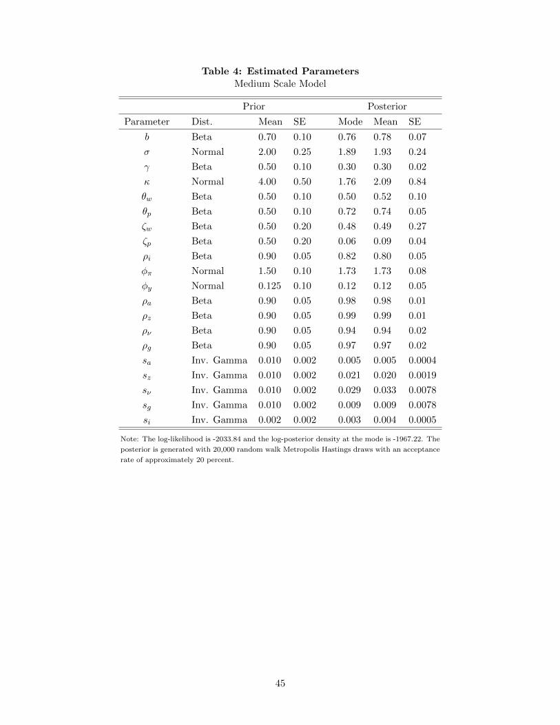
Table 4: Estimated ParametersMedium Scale Model

Prior Posterior

Parameter Dist. Mean SE Mode Mean SE

b Beta 0.70 0.10 0.76 0.78 0.07

σ Normal 2.00 0.25 1.89 1.93 0.24

γ Beta 0.50 0.10 0.30 0.30 0.02

κ Normal 4.00 0.50 1.76 2.09 0.84

θw Beta 0.50 0.10 0.50 0.52 0.10

θp Beta 0.50 0.10 0.72 0.74 0.05

ζw Beta 0.50 0.20 0.48 0.49 0.27

ζp Beta 0.50 0.20 0.06 0.09 0.04

ρi Beta 0.90 0.05 0.82 0.80 0.05

φπ Normal 1.50 0.10 1.73 1.73 0.08

φy Normal 0.125 0.10 0.12 0.12 0.05

ρa Beta 0.90 0.05 0.98 0.98 0.01

ρz Beta 0.90 0.05 0.99 0.99 0.01

ρν Beta 0.90 0.05 0.94 0.94 0.02

ρg Beta 0.90 0.05 0.97 0.97 0.02

sa Inv. Gamma 0.010 0.002 0.005 0.005 0.0004

sz Inv. Gamma 0.010 0.002 0.021 0.020 0.0019

sν Inv. Gamma 0.010 0.002 0.029 0.033 0.0078

sg Inv. Gamma 0.010 0.002 0.009 0.009 0.0078

si Inv. Gamma 0.002 0.002 0.003 0.004 0.0005

Note: The log-likelihood is -2033.84 and the log-posterior density at the mode is -1967.22. The

posterior is generated with 20,000 random walk Metropolis Hastings draws with an acceptance

rate of approximately 20 percent.

45

Table 5: Output and Welfare MultipliersEstimated Medium Scale Model

State Space

Labor Tax Steady State Bad State Bad State Bad State Bad State

Neutral Prod. Investment Preference MP

Output Mult. τn = 1− εpεw(εp−1)(εw−1) 1.211 1.282 1.298 1.280 1.204

τn = 0 1.217 1.289 1.306 1.313 1.213

τn = 0, ρν = 0.65 1.217 1.291 1.196 1.189 1.214

τn = 0, ρg = 0.8 1.306 1.390 1.400 1.413 1.314

Welfare Mult. τn = 1− εpεw(εp−1)(εw−1) 0.230 -0.592 -1.977 -0.369 0.797

τn = 0 3.376 2.678 1.450 2.926 3.847

τn = 0, ρν = 0.65 3.373 2.599 1.403 3.988 3.767

τn = 0, ρg = 0.8 0.835 0.664 0.477 0.747 0.939

This table shows output and welfare multipliers in the medium scale model. These multipliers are generated using the posterior

mean estimates of the parameters shown in Table 4. The different labor taxes in the second column correspond to different levels

of steady state distortion. To compute bad state multipliers, we simulate 1000 periods of data from the model conditional only on

neutral productivity, investment, preference, or monetary policy shocks. We then compute the average value of the state vector for

periods in which realized output is in its lowest decile. We use these average state vectors as the starting positions in computing

impulse responses and multipliers. See the discussion in Footnote 14 for a partial exception to this procedure.

Table 6: Output and Welfare MultipliersEstimated Medium Scale Model, Interest Rate Peg

State Space

Length of Peg Steady State Bad State Bad State Bad State Bad State

Neutral Prod. Investment Preference MP

Output Mult. H = 2 1.329 1.406 1.429 1.414 1.325

H = 3 1.397 1.476 1.503 1.472 1.393

H = 4 1.509 1.589 1.629 1.561 1.505

H = 5 1.742 1.820 1.892 1.724 1.737

H = 6 2.508 2.534 2.800 2.125 2.511

Welfare Mult. H = 2 3.4741 2.7748 1.5603 3.0447 3.9724

H = 3 3.5584 2.8507 1.6446 3.1290 4.0652

H = 4 3.6933 2.9856 1.7964 3.2639 4.2339

H = 5 3.9808 3.2588 2.1085 3.5170 4.5796

H = 6 4.8905 4.0705 3.1627 4.1495 5.7098

This table shows output and welfare multipliers in the medium scale model. We assume that the steady state is distorted,

with all taxes, included τn, equal to zero. These multipliers are generated using the posterior mean estimates of the

parameters shown in Table 4. These multipliers are computed assuming that the interest rate is pegged for H periods,

after which time it follows the standard Taylor rule. To compute bad state multipliers, we simulate 1000 periods of data

from the model conditional only on neutral productivity, investment, preference, or monetary policy shocks. We then

compute the average value of the state vector for periods in which realized output is in its lowest decile. We use these

average state vectors as the starting positions in computing impulse responses and multipliers. See the discussion in

Footnote 14 for a partial exception to this procedure.

46

Table 7: Estimated Parameters: Medium Scale ModelRobustness, Posterior Means

Parameter Add. Separable Var. Tax 1 Var. Tax 2 SS Tax SS Tax Var. 1 SS Tax Var. 2

b 0.74 0.77 0.79 0.76 0.72 0.79

σ n/a 1.87 1.92 1.91 1.88 1.86

γ 0.29 0.30 0.30 0.36 0.36 0.37

κ 2.11 2.12 2.12 2.16 1.74 1.71

θw 0.54 0.51 0.51 0.51 0.48 0.52

θp 0.74 0.74 0.74 0.73 0.70 0.72

ζw 0.48 0.47 0.47 0.46 0.44 0.47

ζp 0.09 0.09 0.08 0.09 0.11 0.13

ρi 0.83 0.81 0.80 0.80 0.80 0.79

φπ 1.75 1.74 1.73 1.75 1.75 1.71

φy 0.14 0.11 0.12 0.12 0.12 0.12

ρa 0.97 0.97 0.97 0.98 0.98 0.98

ρz 0.99 0.99 0.99 0.99 0.99 0.99

ρν 0.92 0.93 0.94 0.93 0.93 0.93

ρg 0.97 0.97 0.97 0.97 0.97 0.97

sa 0.005 0.005 0.005 0.006 0.006 0.005

sz 0.020 0.021 0.020 0.025 0.023 0.023

sν 0.027 0.033 0.033 0.032 0.028 0.032

sg 0.009 0.009 0.009 0.009 0.009 0.009

si 0.003 0.004 0.004 0.004 0.003 0.004

Note: This table shows posterior means for estimations of the medium scale model. In the column labeled “Rest.

pref/gov,” we restrict ρg = 0.8, ρν = 0.65, sg = 0.01, and sν = 0.03. In the columned labeled “Additively separable” we

restrict σ = 1. In the “Cons. Tax” column we assume that variable tax financing is via the distortionary consumption

tax, and estimate the parameters ρc and γc. The columns labeled “Labor Tax” and “Capital Tax” are analogous. The

column labeled “All Taxes” allows all distortionary taxes to react to lagged debt.

47

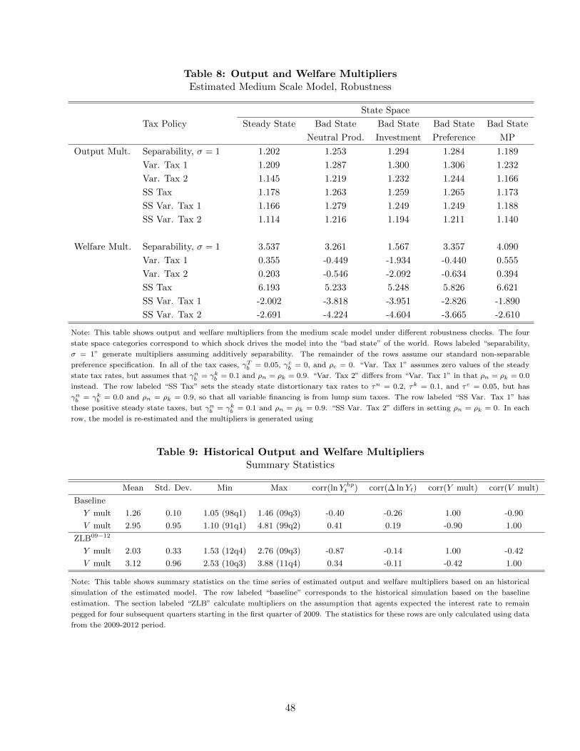
Table 8: Output and Welfare MultipliersEstimated Medium Scale Model, Robustness

State Space

Tax Policy Steady State Bad State Bad State Bad State Bad State

Neutral Prod. Investment Preference MP

Output Mult. Separability, σ = 1 1.202 1.253 1.294 1.284 1.189

Var. Tax 1 1.209 1.287 1.300 1.306 1.232

Var. Tax 2 1.145 1.219 1.232 1.244 1.166

SS Tax 1.178 1.263 1.259 1.265 1.173

SS Var. Tax 1 1.166 1.279 1.249 1.249 1.188

SS Var. Tax 2 1.114 1.216 1.194 1.211 1.140

Welfare Mult. Separability, σ = 1 3.537 3.261 1.567 3.357 4.090

Var. Tax 1 0.355 -0.449 -1.934 -0.440 0.555

Var. Tax 2 0.203 -0.546 -2.092 -0.634 0.394

SS Tax 6.193 5.233 5.248 5.826 6.621

SS Var. Tax 1 -2.002 -3.818 -3.951 -2.826 -1.890

SS Var. Tax 2 -2.691 -4.224 -4.604 -3.665 -2.610

Note: This table shows output and welfare multipliers from the medium scale model under different robustness checks. The four

state space categories correspond to which shock drives the model into the “bad state” of the world. Rows labeled “separability,

σ = 1” generate multipliers assuming additively separability. The remainder of the rows assume our standard non-separable

preference specification. In all of the tax cases, γTb = 0.05, γcb = 0, and ρc = 0. “Var. Tax 1” assumes zero values of the steady

state tax rates, but assumes that γnb = γkb = 0.1 and ρn = ρk = 0.9. “Var. Tax 2” differs from “Var. Tax 1” in that ρn = ρk = 0.0

instead. The row labeled “SS Tax” sets the steady state distortionary tax rates to τn = 0.2, τk = 0.1, and τc = 0.05, but has

γnb = γkb = 0.0 and ρn = ρk = 0.9, so that all variable financing is from lump sum taxes. The row labeled “SS Var. Tax 1” has

these positive steady state taxes, but γnb = γkb = 0.1 and ρn = ρk = 0.9. “SS Var. Tax 2” differs in setting ρn = ρk = 0. In each

row, the model is re-estimated and the multipliers is generated using

Table 9: Historical Output and Welfare MultipliersSummary Statistics

Mean Std. Dev. Min Max corr(lnY hpt ) corr(∆ lnYt) corr(Y mult) corr(V mult)

Baseline

Y mult 1.26 0.10 1.05 (98q1) 1.46 (09q3) -0.40 -0.26 1.00 -0.90

V mult 2.95 0.95 1.10 (91q1) 4.81 (99q2) 0.41 0.19 -0.90 1.00

ZLB09−12

Y mult 2.03 0.33 1.53 (12q4) 2.76 (09q3) -0.87 -0.14 1.00 -0.42

V mult 3.12 0.96 2.53 (10q3) 3.88 (11q4) 0.34 -0.11 -0.42 1.00

Note: This table shows summary statistics on the time series of estimated output and welfare multipliers based on an historical

simulation of the estimated model. The row labeled “baseline” corresponds to the historical simulation based on the baseline

estimation. The section labeled “ZLB” calculate multipliers on the assumption that agents expected the interest rate to remain

pegged for four subsequent quarters starting in the first quarter of 2009. The statistics for these rows are only calculated using data

from the 2009-2012 period.

48

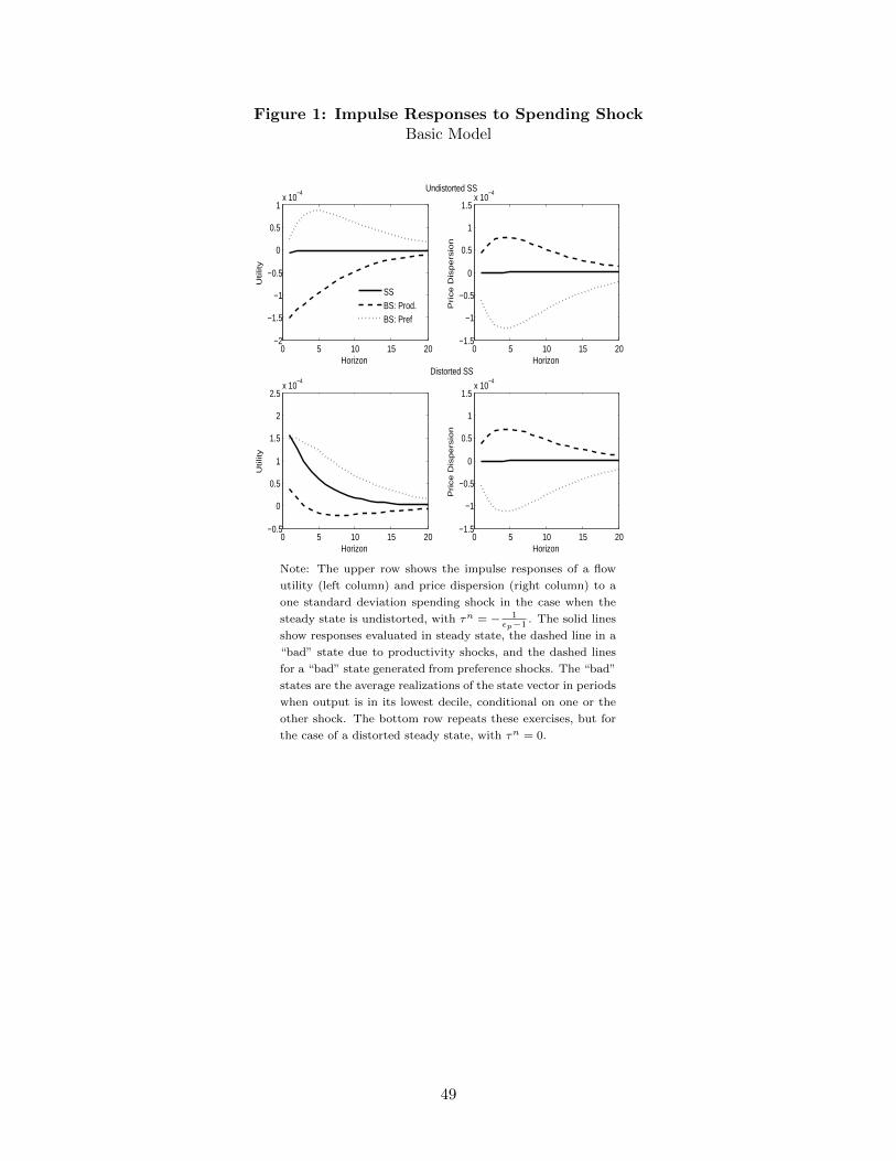
Figure 1: Impulse Responses to Spending ShockBasic Model

0 5 10 15 20−2

−1.5

−1

−0.5

0

0.5

1x 10

−4

Horizon

Utilit

y

SSBS: Prod.BS: Pref

0 5 10 15 20−1.5

−1

−0.5

0

0.5

1

1.5x 10

−4

Horizon

Price

Dis

pe

rsio

n

0 5 10 15 20−0.5

0

0.5

1

1.5

2

2.5x 10

−4

Horizon

Utilit

y

0 5 10 15 20−1.5

−1

−0.5

0

0.5

1

1.5x 10

−4

Horizon

Price

Dis

pe

rsio

n

Undistorted SS

Distorted SS

Note: The upper row shows the impulse responses of a flow

utility (left column) and price dispersion (right column) to a

one standard deviation spending shock in the case when the

steady state is undistorted, with τn = − 1εp−1

. The solid lines

show responses evaluated in steady state, the dashed line in a

“bad” state due to productivity shocks, and the dashed lines

for a “bad” state generated from preference shocks. The “bad”

states are the average realizations of the state vector in periods

when output is in its lowest decile, conditional on one or the

other shock. The bottom row repeats these exercises, but for

the case of a distorted steady state, with τn = 0.

49

Figure 2: Scatter PlotsBasic Model

−0.5 0 0.5 1 1.51

1.05

1.1

1.15

1.2

Welfare Multiplier

Ou

tpu

t M

ultip

lier

−0.1 −0.05 0 0.05 0.11

1.05

1.1

1.15

1.2

Ou

tpu

t M

ultip

lier

Output

Productivity Shocks

−0.1 −0.05 0 0.05 0.1−0.5

0

0.5

1

1.5

We

lfa

re M

ultip

lier

Output

−2 −1 0 1 21

1.05

1.1

1.15

1.2

Welfare Multiplier

Ou

tpu

t M

ultip

lier

−0.05 0 0.051

1.05

1.1

1.15

1.2

Ou

tpu

t M

ultip

lier

Output

Preference Shocks

−0.05 0 0.05−2

−1

0

1

2

We

lfa

re M

ultip

lier

Output

−4 −2 0 2 40.9

1

1.1

1.2

Welfare Multiplier

Ou

tpu

t M

ultip

lier

−0.1 −0.05 0 0.05 0.10.9

1

1.1

1.2

Ou

tpu

t M

ultip

lier

Output

Both Shocks

−0.1 −0.05 0 0.05 0.1−4

−2

0

2

4

We

lfa

re M

ultip

lier

OutputNote: This figures shows scatter plots based on simulations of the basic New Keynesian model

without capital. In all cases the steady state is distorted, with τn = 0. These scatter plots are based

on simulations of 300 periods. In the upper row we generate data when the standard deviation of

preference shocks is set to 0, in the middle panel data are generated conditioning when the standard

deviation of productivity shocks are 0, and the final row is based on a simulation in which both both

productivity and preference shocks are present.

50

Figure 3: Steady State Utility and DistortionsBasic Model

0.26 0.28 0.3 0.32 0.34 0.36 0.38−1.42

−1.415

−1.41

−1.405

−1.4

−1.395

−1.39

−1.385

−1.38

−1.375

N(τ)

U

Note: This figure plots steady state flow util-

ity as a function of steady state hours (which

is in turn a function of the steady state la-

bor tax). Utility is maximized at a tax rate

of τn = − 1εp−1

, which corresponds to steady

state labor hours of 0.347.

51

Figure 4: Multipliers and Length of Interest Rate PegBasic Model

2 4 6 8 10

1.3

1.4

1.5

1.6

1.7

1.8

1.9

2

Ou

tpu

t M

ultip

lier

Length of Peg

Productivity Shocks

SS, UndistortedSS, DistortedBS, UndistortedBS, Distorted

2 4 6 8 10

1.3

1.4

1.5

1.6

1.7

1.8

1.9

2

Ou

tpu

t M

ultip

lier

Length of Peg

Preference Shocks

2 4 6 8 10−1.5

−1

−0.5

0

0.5

1

We

lfa

re M

ultip

lier

Length of Peg2 4 6 8 10

−1

0

1

2

3W

elfa

re M

ultip

lier

Length of PegNote: These figures plot the output and welfare multipliers (vertical axes, output multipliers in the

upper row and welfare multipliers in the bottom row)) as a function of the length of an interest

rate peg (horizontal axis). The solid lines are the multipliers evaluated in an undistorted steady

state, where τn = − 1εp−1

. The solid lines with + signs are the multipliers evaluated in a distorted

steady state, where τn = 0. In the left column are multipliers evaluated in “bad” states generated

by productivity shocks. In the right column are multipliers in “bad” states generated by preference

shocks. The dashed lines show the multipliers in the bad state when the steady state is undistorted.

The dotted lines plot the multipliers as a function of the peg in a bad state where the steady state

is distorted.

52

Figure 5: Historical Output and Welfare MultipliersMedium Scale Model

0.9

1.0

1.1

1.2

1.3

1.4

1.5

1.6

1.7

1.0

1.5

2.0

2.5

3.0

3.5

4.0

4.5

5.0

86 88 90 92 94 96 98 00 02 04 06 08 10 12

Output MultiplierWelfare Multiplier

Outp

ut M

ulti

plie

rW

elfa

re M

ultip

lier

Note: This figure plots the estimated historical output and welfare multipliers. Shaded

gray regions are recessions as dated by the NBER. These simulations are based on using

the Kalman smoother from the estimated model to back out a history of states. Then at

each point in the state space, we compute the output and welfare multipliers.

53

Figure 6: Historical Output and Welfare MultipliersMedium Scale Model, Zero Lower Bound Period

1.2

1.4

1.6

1.8

2.0

2.2

2.4

2.6

2.8

2.0

2.4

2.8

3.2

3.6

4.0

4.4

4.8

5.2

I II III IV I II III IV I II III IV I II III IV I II III IV I II III IV

2007 2008 2009 2010 2011 2012

Output MultiplierWelfare Multiplier

Out

put M

ultip

lier W

elfare Multiplier

Zero lower bound period

Note: This figure plots the estimated historical output and welfare multipliers taking the

zero lower bound on interest rates into account. The shaded gray region corresponds to the

period in which we assume agents began to expect interest rates to remain fixed. These

simulations are based on using the Kalman smoother from the estimated model to back

out a history of states. Then at each point in the state space, we compute the output and

welfare multipliers assuming that, at each date, agents expected nominal interest rates to

be pegged at their lagged value for the ensuring four quarters.

54