6

EUROPEAN ECONOMY

Economic and Financial Affairs

ISSN 2443-8022 (online)

EUROPEAN ECONOMY

MacroeconomicEffects ofFiscal Shocksin Portugal

Elva Bova and Violeta Klyviene

DISCUSSION PAPER 096 | MAY 2019

European Economy Discussion Papers are written by the staff of the European Commission’s Directorate-General for Economic and Financial Affairs, or by experts working in association with them, to inform discussion on economic policy and to stimulate debate. The views expressed in this document are solely those of the author(s) and do not necessarily represent the official views of the European Commission. Authorised for publication by Carlos Martínez Mongay, Director for Economies of the Member States II.

LEGAL NOTICE Neither the European Commission nor any person acting on behalf of the European Commission is responsible for the use that might be made of the information contained in this publication. This paper exists in English only and can be downloaded from https://ec.europa.eu/info/publications/economic-and-financial-affairs-publications_en. Luxembourg: Publications Office of the European Union, 2019 PDF ISBN 978-92-79-77433-1 ISSN 2443-8022 doi:10.2765/100789 KC-BD-18-023-EN-N

© European Union, 2019 Non-commercial reproduction is authorised provided the source is acknowledged. For any use or reproduction of material that is not under the EU copyright, permission must be sought directly from the copyright holders.

European Commission Directorate-General for Economic and Financial Affairs

Macroeconomic Responses to Fiscal Shocks in Portugal Elva Bova and Violeta Klyviene Abstract This study analyses the impact of fiscal shocks on GDP, inflation and interest rates in Portugal over 1995-2017. In line with the relevant literature, we estimate multipliers using a structural VAR a' la Blanchard and Perotti (2002) based on OECD elasticities. As fiscal shocks, we include changes in direct and indirect taxes on the revenue side, and, on the expenditure side, changes in public consumption, investment and transfers. We find small tax multipliers and larger government consumption multipliers for growth, while short-term responses to shocks in transfer and investment spending are found to be negligible. We find an ambiguous impact of fiscal shocks on inflation, with both indirect and direct taxes having an inflationary impact but government consumption having the contrary impact. Fiscal shocks of an expansionary nature are found to trigger declines in real interest rates, possibly through the inflation channel. The results are robust to different orderings of the variables used in the structural VAR and to the selection of alternative time periods. Overall, the analysis of output multipliers compares well with some other studies conducted on the Portuguese economy and confirms the importance of the disposable income channel in the transmission of fiscal shocks to the rest of the economy. JEL Classification: E62, H3, C20. Keywords: Fiscal shocks, structural VAR, Portugal. Acknowledgements: The authors are grateful to Carlos Martínez-Mongay, Christian Weise and Martin Hallet for their very valuable comments. They also would like to thank Francisco De Castro and Aurelien Poissonnier for excellent peer review. Contact: Elva Bova, European Commission, Directorate-General for Economic and Financial Affairs, elva.bova@ec.europa.eu; Violeta Klyviene, European Commission, Directorate-General for Economic and Financial Affairs, violeta.klyviene@ec.europa.eu.

EUROPEAN ECONOMY Discussion Paper 096

CONTENTS

3

1. Introduction 5

2. Literature review 7

3. Methodology 13

4. Data 17

5. Empirical results 21

6. Conclusion 29

REFERENCES 31

ANNEX 1 35

LIST OF TABLES 2.1. Fiscal multipliers in Portugal 8 2.2. Fiscal multipliers in the OECD (selected studies) 9 4.1. Elasticities of revenue and spending components 18 5.1. Impulse response coefficients to a 1% shock 22 5.2. Cumulated fiscal multipliers: disaggregated approach 23 5.3. Impulse response coefficients with inverted order 25 5.4. Cumulated fiscal multipliers: 1995-2008 26 5.5. Impulse response coefficients: 1999-2017 26 A1.1. Unit root test results 35 A1.2. Lag determination test results 35

LIST OF GRAPHS 5.1. GDP impulse responses to tax shocks in the three SVARs model specifications 27 A1.1. Accumulated response of macro variables to a 1% shock in tax variables 36 A1.2. Accumulated response of macro variables to a 1% shock in expenditure variables 37

4

1. INTRODUCTION

5

This study analyses the impact of fiscal shocks on the Portuguese economy. We identify the response of GDP, inflation and interest rates to changes in public expenditure and revenue over 1995-2017. The study provides impulse responses over a horizon of four years, which allows examining the short-term impact and the persistence of the impact over time. In line with the relevant literature, we estimate multipliers using a structural VAR where restrictions have been imposed following Blanchard and Perotti (2002) and we use OECD elasticities for the estimation. While the analysis of output multipliers compares well with some other studies conducted on the Portuguese economy, our study is one of the first to focus also on the implications of fiscal shocks on inflation and long term interest rates. This side of the analysis is relevant for countries, like Portugal, that display high debt levels and volatile market sentiment and lack an independent monetary policy.

Our main findings are the following:

• Growth dynamics in Portugal are sensitive to shocks in government consumption, which are found to trigger positive, relatively large and persistent output responses. We find a negative reaction of output to increases in direct taxes, although this impact is small and short-lived. Increases in indirect taxes trigger unstable and largely insignificant output reactions, possibly due to quite inelastic consumption patterns in the country. Output responses to changes in public investment are found to be negligible, possible on account of the very short-term horizon within which the impact is estimated, while responses to transfers are small, short-lived and negative.

• The impact of fiscal shocks on inflation is ambiguous. Indirect tax shocks have some pass-through on prices, as expected, but also direct taxes are found to raise inflation. While government transfers and investments would trigger increases in inflation, public consumption is found to trigger decreases in inflation.

• Contrary to what is usually believed but consistent with previous studies (Perotti 2002), fiscal shocks of an expansionary nature are found to trigger declines in interest rate, which could be in part explained by the inflation impact on real interest rates.

The results are robust to different orderings of the variables used in the structural VAR, and also to the selection of an alternative time period which excludes the financial crisis. The results on growth dynamics are broadly consistent with findings from the literature, and also from other studies on Portugal which find disposable income to be an important channel through which fiscal policy is transmitted to output, mainly through government consumption. To our knowledge, the results on inflation and on the interest rates are indeed quite novel for Portugal and call for further investigation on the topic.

This study is structured as follows. Section two provides a review of the literature on fiscal shocks and multipliers with a focus on studies on Portugal and how they compare with studies on other OECD countries. Section three reviews the methodology employed while section four provides information on the data used for the estimation. In section five we provide the results of the empirical estimation and section six concludes the paper.

2. LITERATURE REVIEW

7

Understanding the size, sign and determinants of fiscal multipliers in a specific economy is a crucial tool for policy design, as it allows assessing the impact of discretionary revenue and expenditure policies on output and other macro-related variables. The literature defines fiscal multipliers as the ratio of a change in output to a discretionary change in government spending or tax revenue (Spilimbergo et al. 2009).

Output responses A vast literature has tried to identify fiscal multipliers on growth. Several methodologies have been considered, reflecting different attempts to distinguish between changes in automatic stabilisers and changes in discretionary fiscal policy responses. Distinguishing between the two types of changes in fiscal variables has made the estimation of multipliers extremely hard. As a consequence, consensus on the size of the multipliers is still lacking (Batini et al. 2014). In the context of advanced economies, the most common methodologies used to estimate fiscal multipliers have been Dynamic Stochastic General Equilibrium (DSGE) simulations (Coenen et al. 2012; Woodford 2011; Christiano et al. 2011), Structural Vector Autoregressive (SVAR) models and the narrative approach based on historical information on fiscal policy shocks (Romer and Romer 2010; Ramey 2011). The structural VAR methodology, used in this study, relies on empirical time series data to estimate the multipliers. To limit the endogeneity issue that could emerge from inverse causality from growth to fiscal variables rather than the direction examined from fiscal variables to growth, this methodology uses the elasticities of expenditure and revenue to separate the impact of automatic stabilisers from that one of exogenous fiscal shocks.

Despite the wide variety of results and specifications found by these studies, some common features can still be summarised (see also Mineshima et al. 2014). First year multipliers in normal times are found to range between 0 and 1. When the economy is undergoing a downturn, then the size of the multipliers is larger than under expansions, both for fiscal stimulus and consolidation (Auerbach and Gorodnichenko 2012). Also, the degree of monetary accommodation to fiscal shocks plays a role, as at the zero lower bound multipliers tend to be large (Woodford 2011). Studies converge regarding the different size of multipliers for each component of the fiscal balance. Spending multipliers tend to be larger than revenue multipliers. Within the former, investment spending has usually the largest impact on output, followed by government consumption of goods and services and the wage bill. On the contrary, evidence on transfers is mixed and might be due to the different impact of targeted transfers (high impact) and untargeted (low impact). On the revenue side, direct taxes have usually a higher multiplier (corporate taxes more than labour taxes), while indirect taxes, especially on consumption, have a lower impact (Batini et al. 2014).

Cross-country comparisons of multiplier estimates highlight how some specific characteristics can increase or reduce the impact of fiscal shocks on output. Looking at a sample of 44 countries, Ilzetzki et al. (2011) find that the level of development, the degree of flexibility of the exchange rate, trade openness and public indebtedness matter for the transmission of fiscal shocks to the economy. As such, they indicate that fiscal multipliers tend to be larger in advanced economies under fixed exchange rates, in closed economies rather than open ones and in low-debt countries. For the case of Portugal, this would imply a higher than average multiplier due to the fixed exchange rate, but probably a lower than average multiplier based on high debt and the high degree of openness.

Several studies have investigated the size and sign of fiscal multipliers in Portugal, reaching different results (Table 2.1). Using a Bayesian structural autoregression model, Afonso and Sousa (2011) find that an increase in government spending has a negative effect on real GDP. Such finding is contrary to most studies on the expenditure multipliers, which find instead a positive GDP impact

8

of an increase in spending and it is here justified by the crowding-out effect of public spending on the private sector and the impact that higher spending can have on financing costs for debt. At the same time, they also find that an increase in revenue has a negative impact on private consumption and private investment although with a much longer lag than the impact of spending on output. Based on a DSGE analysis, Castro et al. (2013) test for multipliers in Portugal under normal times and under crisis times, where the latter feature a higher share of budget-constrained households, stronger nominal rigidities, and more severe financial frictions. They find that fiscal multipliers can be twice as large in crisis times, especially for government consumption, where a decline would largely and more durably impact growth. They also find that government consumption multipliers are larger than transfers and taxes, but find no difference between labour and consumption taxes in the short-run. These findings are in line with Poirier (2014) who applies a threshold VAR to identify Portuguese fiscal multipliers at periods of recession and expansion. Examining quarterly data from 1991 to 2013, they find larger and more persistent spending multipliers than tax multipliers. In line with some other studies on regime switching (Auerbach and Gorodnichenko 2012), they also find that multipliers are much larger under recessions and that tax hikes can slow down growth.

Table 2.1: Fiscal multipliers in Portugal

(1) One-year impact only. (2)* For Castro et al. (2013) we report the multipliers of the baseline effect, hence net of financial frictions. The multipliers are here calculated as percentage change of real GDP to a one percent of GDP change in the fiscal variable. (3)** In Pereira and Wemans (2013) results are reported for shocks normalised to have the size of one euro (increase or decline). (4) ***In Pereira and Roca-Sagalés (2011), the multipliers are calculated with respect to a euro increase or decline in the fiscal variable and reflect the average long-term impact of a shock over 10 years. In our study we use the euro-based specification also used in Pereira and Roca-Sagalés. Although the size of the coefficients of the other two studies would not be directly comparable to ours, the relative size of each fiscal variable coefficient remains of interest for our analysis Source: Pereira and Roca-Sagalés (2011), Castro et al. (2013), Pereira and Wemans (2013), Poirier (2014)

To identify the impact of specific categories of spending and taxes, a study by Pereira and Roca-Sagalés (2011) applies an unrestricted VAR (using the recursive approach (1)) on annual data in real terms for the 1980-2005 period. On the spending side, they find a large multiplier for public wages, followed by public transfers while the multiplier for public investment is just more than half the one of wages. On the revenue side, they find a stronger multiplier for direct taxation, and a negligible effect of indirect taxes. These findings are in line with Pereira and Wemans (2013), who conduct an analysis on quarterly government account data for 1995-2011. Using a structural VAR, they look at multipliers per budget category and find stronger multipliers for compensation of employees and direct taxes. These are not only larger in size but more persistent over time, with salaries more persistent than taxes. On the contrary, transfers and indirect taxes are found to have a (1) A structural VAR is preferable to an unrestricted VAR which presents significant limitations. Unrestricted VARs

in fact tend to miss nonlinearities, conditional heteroskedasticity, and drifts or breaks in parameters.

Pereira and Roca-Sagalés (2011)***

Castro et al. (2013)*

Pereira and Wemans (2013)**

Poirier (2014)

Spending multiplier 1.2 1.2Government consumption 0.62 1.0

Transfers 1.81 0.5 0.5Government investment 4.7

Revenue multiplier -1.8 0.01Direct taxes -2.78 -0.6Labour taxes -0.5

Consumption taxes -0.18 -0.5 0.0

9

smaller impact. Interestingly, they find a counterintuitive sign for the impact of expenditure on goods and services (including also investment) on output. Overall, they conclude that disposable income is indeed an important transmission mechanism from fiscal policy to the economy in Portugal.

Table 2.2: Fiscal multipliers in the OECD (selected studies)

(1) The range for Blanchard and Perotti (2002) estimates depend on whether a deterministic or a stochastic trend is included Source: Blanchard and Perotti (2002), Perotti (2002), Mountford and Uhlig (2002), Perotti (2004), Biau and Girard (2005), De Castro (2006), Romer and Romer (2010), Baum and Koester (2011), Cleaud et al. (2013), Mertnes and Ravn (2013), Hayo and Uhl (2014)

How do the multipliers of these studies compare with multipliers found in other OECD countries? Table 2.2 presents a selection of studies whose methodologies and definition of multipliers are comparable in nature and whose samples are interesting for the case of Portugal.(2) With a first year spending multiplier around 1.21, the coefficient for Portugal is similar to what other studies find for Southern European countries (Table 2.2). For France, for example, Biau and Girard (2005) obtain a spending multiplier of 1.4 and Cleaud et al. (2013) obtain a multiplier of 1.1. For Italy, the spending multiplier is around 1.2 in Giordano et al. (2007), while for Spain it amounts to between 1.14 and 1.54 (De Castro 2006). For the US, the UK and Germany, the multipliers are lower than in Portugal. On the US, in particular, studies find a multiplier ranging from 0.01 and 0.3. For Germany, Perotti (2) By presenting the results in a different format than the ones reported in the tables, some other studies considered

in this paper have not been reported in the table, for example Guajardo et al. (2014) using a panel of 17 OECD economies, Favero and Giavazzi (2012) for the USA, Heppke-Falk et al. (2006) for Germany and de Castro and Hernández de Cos (2008) and de Castro and Fernandez (2013) for Spain.

Estimation Sample Country Revenue multipliers

Spending multiplier

Net tax multiplier

Blanchard and Perotti (2002) SVAR 1947-1997 USA -0.74*/-1.07* 0.45/0.55

Perotti (2002) SVAR 1964-2000 Australia 0.44* 0.01

Perotti (2002) SVAR 1961-2000 USA -0.66* 0.29

Perotti (2002) SVAR 1961-1989 West Germany -0.46* 0.96*

Perotti (2002) SVAR 1962-2001 Canada -0.48* 0.06

Perotti (2002) SVAR 1964-2001 UK 0.05 -0.04

Mountford and Uhlig (2002) SVAR 1955-2000 USA 1.95 0.5

Mertnes and Ravn (2013) narrative approach 1950-2006 USA -1

Romer and Romer (2010) narrative approach 1945-2007 USA -1.2

Perotti (2004) SVAR 1960-1974 Germany 0.53 0.29

Perotti (2004) SVAR 1975-1989 Germany 0.5 -0.04

Hayo and Uhl (2014) Germany -1

Baum and Koester (2011) Threshold-VAR 1976-2009 Germany -0.66 0.7

Biau and Girard (2005) SVAR 1978-2003 France 1.4 -0.1

Cleaud et al. (2013) SVAR 1980-2010 France 1.1

Giordano et al. (2007) SVAR 1982-2004 Italy 1.2 0.16

De Castro (2006) SVAR 1980-2001 Spain 1.14 - 1.54 0.05

Perotti (2002) UK 0.04

Cloyne (2013) narrative approach 1945-2009 UK -0.6

10

(2002, 2004) finds a multiplier between 0.5 and 0.96, and for the UK the multiplier is around 0.4 (Perotti 2004). The difference among these spending multiplier coefficients seems to invalidate the prediction that low debt countries would have a larger multiplier, as Southern European countries should then tend to have smaller multipliers. It actually reinforces the point in favour of the importance of a fixed exchange rate in the transmission mechanism from fiscal policy to the economy, as euro area countries have a higher multiplier. The picture is rather different for the revenue multiplier, which in the studies examined ranges largely from -1.8 to 0.01, hence limiting a sound comparison with other studies.

Price responses The literature on the impact of fiscal policy on prices and inflation is not as broad. A study by Henry et al. (2004) provides a comprehensive review. Their review of the literature points to inconclusive results regarding the impact of tax shocks, where taxes or even revenues are considered in aggregate and not distinguished by component. Several explanations are advanced to explain these mixed results. Considering direct taxation, an increase in taxes might on the one hand dampen aggregate demand by decreasing household income, hence decreasing prices, and, on the other hand, it can increase prices by raising labour costs for firms. For indirect taxes, the main underlying theoretical assumption is that their increase can directly be passed-through on consumers, hence on prices. This impact might also be strengthened if workers ask for wage adjustments to changes in prices, thereby increasing labour costs and in turn prices.

Regarding expenditure, Henry et al. (2004) report mixed results from the review of the literature. Some studies do indeed find a negative impact on prices after an increase in government spending (Fatas and Mihov 2001; Mountford and Uhlig 2009); while others find the opposite (Perotti 2002, Marcellino 2002 on France, Canova and Pappa 2002). Such difference in impact is explained by whether the shock is a supply or demand shock: whether an increase in expenditure would stimulate demand and hence a price increase, or it would instead stimulate production and, through this, it would lower prices.

Interest rate responses Like for inflation multipliers, the literature on the impact of fiscal policy on the interest rate is not as broad as the one on growth multipliers. Considering the deficit at large, the theory claims that an increase (decrease) in the deficit could at the same time result in an increase (decrease) in the interest rate or in a decrease (increase). In the first case, when deficits and interest rates move in the same direction, it is more commonly argued that fiscal profligacy could deteriorate market sentiment and investors would opt for other options than government bonds, hence increasing their interest rates. In extremis, this argument has been also labelled as the 'bond vigilantes' prediction (Krugman 2012), and applied to explain changes in the euro area spreads at the core of the euro area crisis. In the second case, when the deficit and interest rate move in opposite directions, the theory would interpret this finding as a result of a coordinated and contemporaneous change in fiscal and monetary policies, and not as the impact of changes in the deficit on interest rates. As expressed in Perotti (2002), increases in interest rates may go along with a reduction in expenditure when a country is undergoing a joint fiscal and monetary tightening; and the contrary would apply in case of a macroeconomic loosening. In the case of Portugal or any euro area country, this could clearly imply that fiscal policy is being tuned with the ECB monetary policy stance.

Such divergence in the theory justifies mixed evidence regarding the relationship between interest rates and fiscal policy, as reported by Gale and Orszag (2002) and more recently by Laubach (2011). Gale and Orszag in their review of the literature found a positive impact of an increase in the deficit on interest rates in about half of the studies examined and insignificant or mixed results for the rest

11

of the studies. Laubach found that there is a clear link between time variation in risk aversion and the sensitivity of EMU government bond spreads to the fiscal position of individual countries, but this non-linear effect is difficult to capture by standard models. On the other hand, not only fiscal variables but other country-specific factors not captured by our note might also be important. In some other cases, the relationship between fiscal policy and interest rates is better captured by using fiscal projections rather than actual data (Dell'Erba and Sola 2011). Arguably, when interest rates are expressed in real terms, as it is the case in this study, an important channel to take into account would be the inflation impact on the real rates.

3. METHODOLOGY

13

The basic VAR model includes six variables: GDP (Y), inflation (P), Interest rates (I), indirect taxes (T1), direct taxes and social contributions (T2) and government spending and transfers (G). All variables are seasonally adjusted and all fiscal variables expressed in real terms using the GDP deflator. We decide to specify the model in first difference to avoid any spurious regression that might emerge if one of the series is non-stationary. The standard VAR has the following formula:

𝑋𝑋𝑡𝑡 = Γ0 + ∑ ΓiXt−i𝑝𝑝𝑖𝑖=1 + 𝑈𝑈𝑡𝑡, (1)

where 𝑋𝑋𝑡𝑡 is a k×1 vector of the logs of endogenous variables and Γ0 is a k×1 vector of constants, 𝑈𝑈𝑡𝑡 is a k×1 vector of reduced form residuals (𝑢𝑢𝑡𝑡𝑌𝑌 𝑢𝑢𝑡𝑡𝑃𝑃 𝑢𝑢𝑡𝑡𝐼𝐼 𝑢𝑢𝑡𝑡𝑇𝑇1 𝑢𝑢𝑡𝑡𝑇𝑇2 𝑢𝑢𝑡𝑡𝐺𝐺)′ and Γi is a k×k matrix.

The standard VAR estimation cannot unravel the contemporaneous interrelations as the standard residuals are not pure random shocks to the relevant variables. In order to overcome this, we use structural VAR (SVAR) estimation methods and impose some restrictions.

The identification strategy used is based on the Blanchard-Perotti method (2002), according to which fiscal shocks are identified by imposing contemporaneous restrictions on the 𝑈𝑈𝑡𝑡 vector in order to derive a vector of ‘structural’ fiscal shocks, orthogonal to each other and to the other non-fiscal shocks of the model. In the context of fiscal policy, such identification procedure allows in turn to separate at least in part the reaction related to automatic stabilisers which would usually have a contemporaneous change to output and the one related to discretionary fiscal policy changes. From this point an AB model, where a linear relation is assumed to hold between the reduced form residuals and the structural shocks, is used:

𝐴𝐴𝑈𝑈𝑡𝑡 = 𝐵𝐵Ψ𝑡𝑡, (2)

where B is a 6 dimensional matrix of structural shock coefficients and Ψ𝑡𝑡 is a 6 dimensional vector of structural shocks (𝜀𝜀𝑡𝑡𝑌𝑌 𝜀𝜀𝑡𝑡𝑃𝑃 𝜀𝜀𝑡𝑡𝐼𝐼 𝜀𝜀𝑡𝑡𝑇𝑇1 𝜀𝜀𝑡𝑡𝑇𝑇2 𝜀𝜀𝑡𝑡𝐺𝐺)′ (see Lütkepohl 2005).

According to the Blanchard-Perotti approach, the estimation procedure of the SVAR model is divided into four steps: the estimation of the unrestricted VAR, the identification of its reduced form, the ordering of the variables and finally the estimation of the parameters. The estimation of the unrestricted VAR takes the form of six equations in our case and is estimated using a simple OLS. In the second step, we express the reduced form innovations of every fiscal variable as linear combinations of the three types of shocks: (a) the automatic response of the fiscal variables to GDP, inflation and interest rate innovations; (b) the discretionary response of fiscal variables to shocks to macro variables; and (c) structural shocks that are of the main importance to us. Thus, formula (2) can be transformed into these:

𝑢𝑢𝑡𝑡𝑇𝑇1 = 𝛼𝛼𝑌𝑌𝑇𝑇1𝑢𝑢𝑡𝑡𝑌𝑌 + 𝛼𝛼𝑃𝑃𝑇𝑇1𝑢𝑢𝑡𝑡𝑃𝑃 + 𝛼𝛼𝐼𝐼𝑇𝑇1𝑢𝑢𝑡𝑡𝐼𝐼 + 𝛽𝛽𝑇𝑇2𝑇𝑇1𝜀𝜀𝑡𝑡𝑇𝑇2 + 𝛽𝛽𝐺𝐺𝑇𝑇1𝜀𝜀𝑡𝑡𝐺𝐺 + 𝜀𝜀𝑡𝑡𝑇𝑇1, (3)

𝑢𝑢𝑡𝑡𝑇𝑇2 = 𝛼𝛼𝑌𝑌𝑇𝑇2𝑢𝑢𝑡𝑡𝑌𝑌 + 𝛼𝛼𝑃𝑃𝑇𝑇2𝑢𝑢𝑡𝑡𝑃𝑃 + 𝛼𝛼𝑇𝑇1𝑇𝑇2𝑢𝑢𝑡𝑡I + 𝛽𝛽𝑇𝑇1𝑇𝑇2𝜀𝜀𝑡𝑡𝑇𝑇1 + 𝛽𝛽𝐺𝐺𝑇𝑇2𝜀𝜀𝑡𝑡𝐺𝐺 + 𝜀𝜀𝑡𝑡𝑇𝑇2, (4)

𝑢𝑢𝑡𝑡𝐺𝐺 = 𝛼𝛼𝑌𝑌𝐺𝐺𝑢𝑢𝑡𝑡𝑌𝑌 + 𝛼𝛼𝑃𝑃𝐺𝐺𝑢𝑢𝑡𝑡𝑃𝑃1 + 𝛼𝛼𝐼𝐼𝐺𝐺𝑢𝑢𝑡𝑡I + 𝛽𝛽𝑇𝑇1𝐺𝐺 𝜀𝜀𝑡𝑡𝑇𝑇1 + 𝛽𝛽𝑇𝑇2𝐺𝐺 𝜀𝜀𝑡𝑡𝑇𝑇2 + 𝜀𝜀𝑡𝑡𝐺𝐺. (5)

The parameters αij are the exogenous elasticity of the fiscal variables to the macro variables (Y, P, I)

and represent the automatic response of fiscal variables to a changing macro environment. The parameters βi

jestimate the impact of the structural and fiscal shocks on each other. According to the Blanchard-Perotti methodology (2002), the fiscal authorities need more than one quarter to adjust

14

fiscal variables as a reaction to macroeconomic developments. Thus, the discretionary response of fiscal policy to macroeconomic conditions is restricted to 0. In order to compute cyclically adjusted reduced-form fiscal policy shocks based on the Blanchard and Perotti (2002) approach, exogenous elasticities αi

j are used. The elasticities of fiscal variables to interest rate innovations were set to zero, while to output and inflation innovations were calculated based on the OECD (see section 4).

To assess the size of fiscal multipliers, the change in a fiscal variable should be distinguished between the cyclical change, i.e. the change directly triggered by macroeconomic variables, and discretionary changes, which are those that can better capture fiscal policy shocks. This is the second step of the estimates. The parameters of equations 3-5 cannot be estimated by the usual OLS because the reduced form residuals and structural shocks are correlated. Instead, in the following step, exogenous elasticities α_i^j are used in order to compute cyclically adjusted reduced-form fiscal policy shocks. The cyclically adjusted and reduced-form fiscal policy shocks can be specified as follows:

𝑢𝑢𝑡𝑡𝑇𝑇1′ = 𝑢𝑢𝑡𝑡𝑇𝑇1 − 𝛼𝛼𝑌𝑌𝑇𝑇1𝑢𝑢𝑡𝑡𝑌𝑌 − 𝛼𝛼𝑃𝑃𝑇𝑇1𝑢𝑢𝑡𝑡𝑃𝑃 + 𝛼𝛼𝐼𝐼𝑇𝑇1𝑢𝑢𝑡𝑡𝐼𝐼 = 𝛽𝛽𝑇𝑇2𝑇𝑇1𝜀𝜀𝑡𝑡𝑇𝑇2 + 𝛽𝛽𝐺𝐺𝑇𝑇1𝜀𝜀𝑡𝑡𝐺𝐺 + 𝜀𝜀𝑡𝑡𝑇𝑇1, (6)

𝑢𝑢𝑡𝑡𝑇𝑇2′ = 𝑢𝑢𝑡𝑡𝑇𝑇2 − 𝑢𝑢𝑡𝑡𝑌𝑌 + 𝛼𝛼𝑃𝑃𝑇𝑇2𝑢𝑢𝑡𝑡𝑃𝑃 + 𝛼𝛼𝐼𝐼𝑇𝑇2𝑢𝑢𝑡𝑡I = 𝛽𝛽𝑇𝑇1𝑇𝑇2𝜀𝜀𝑡𝑡𝑇𝑇1 + 𝛽𝛽𝐺𝐺𝑇𝑇2𝜀𝜀𝑡𝑡𝐺𝐺 + 𝜀𝜀𝑡𝑡𝑇𝑇2, (7)

𝑢𝑢𝑡𝑡𝐺𝐺′ = 𝑢𝑢𝑡𝑡𝐺𝐺 − 𝛼𝛼𝑌𝑌𝐺𝐺𝑢𝑢𝑡𝑡𝑌𝑌 − 𝛼𝛼𝐼𝐼𝐺𝐺𝑢𝑢𝑡𝑡I = 𝛽𝛽𝑇𝑇1𝐺𝐺 𝜀𝜀𝑡𝑡𝑇𝑇1 + 𝛽𝛽𝑇𝑇2𝐺𝐺 𝜀𝜀𝑡𝑡𝑇𝑇2 + 𝜀𝜀𝑡𝑡𝐺𝐺. (8)

In the third step, in order to identify the structural shocks to fiscal variables, a decision with respect to the ordering of the fiscal variables can be taken. In this paper, it was assumed that the spending decision comes first. In general, there is no strong empirical evidence to support the priority of a tax decision. This seems to be however justified in Portugal because like in many other countries spending decisions are taken before information on the actual performance of the economy is available to the authorities. This ordering is consistent with Blanchard and Perotti (2002) and De Castro (2006). In particular, Blanchard and Perotti (2002) find that the correlation between government revenue and spending is rather small and hence, it does not have a great impact on the results. Taking into account the assumptions that the decision about expenditure is taken first, the following restriction has been imposed: 𝛽𝛽𝑇𝑇1𝑇𝑇2 = 𝛽𝛽𝑇𝑇1𝐺𝐺 = 𝛽𝛽𝑇𝑇2𝐺𝐺 = 0 (3). The first restriction means that any indirect tax shock cannot be quickly (at the same period) transmitted to the labour and capital taxes. The other two restrictions mean that both tax revenue shocks at the same time cannot affect public spending.

𝑢𝑢𝑡𝑡𝐺𝐺′ = 𝜀𝜀𝑡𝑡𝐺𝐺, (9)

𝑢𝑢𝑡𝑡𝑇𝑇2′ = 𝛽𝛽𝐺𝐺𝑇𝑇2𝜀𝜀𝑡𝑡𝐺𝐺 + 𝜀𝜀𝑡𝑡𝑇𝑇2, (10)

𝑢𝑢𝑡𝑡𝑇𝑇1′ = 𝛽𝛽𝑇𝑇2𝑇𝑇1𝜀𝜀𝑡𝑡𝑇𝑇2 + 𝛽𝛽𝐺𝐺𝑇𝑇1𝜀𝜀𝑡𝑡𝐺𝐺 + 𝜀𝜀𝑡𝑡𝑇𝑇1. (11)

The estimation of the non-restricted βs is made by carrying out OLS recursively.

In a final stage, after the fiscal shocks were defined, the remaining parameters of the macroeconomic variables (utI; utP; utY) were estimated using the following specification:

(3) This is a technical assumption and the inverse restriction is also possible without significant effects on the

estimates.

15

utI = αT1I utT1 +αT2I utT2 + αGI utG + εtI (12)

utP = αYPutY + αIPutI + αT1P utT1 +αT2P utT2 + αG PutG + εtP, (13)

utY = αPYutP + αIYutI + αT1Y utT1 + αT2Y utT2 + αGYutG + εtY. (14)

The regressions 12 to 14 cannot be estimated by the usual OLS because, again, the error terms are correlated with the regressors. Therefore, the estimation is carried out by applying the instrumental variables technique recursively using the structural shocks of previous equations as instruments. Since the structural shocks εt are orthogonal, they can be used as instruments.

4. DATA

17

In the benchmark SVAR model three macro and three fiscal variables have been used: real GDP, HICP inflation, the nominal interest rate of ten-year government bonds, direct taxes, indirect taxes and government spending. For tax revenue, it was decided to distinguish direct taxes from indirect taxes in order to capture differences in the potential economic efficiency gain/loss from the trade-off between direct and indirect taxes. Direct taxes in this paper do not meet the standard concept as they include not only corporate and personal income taxes but also social contributions. In general, social contributions could be treated as taxes due to the relatively large element of redistribution in the social security system. The indirect tax definition is in line with ESA 2010. As regards government spending, three separate shocks (hence three separate SVARs) were carried out including government consumption, investment and transfers. Within this, government consumption includes intermediate consumption (about 6% of GDP in 2016) and the public wage bill (about 11% of GDP). Public investment is about 2% of GDP and excludes investment conducted through PPPs, which for the period 1990-2011 amounted to about 1% of GDP, and was recorded either off balance sheet or if on balance sheet it was recorded as part of intermediate consumption. Transfers (about 19% of GDP in 2016) include low impact variables, such as transfers to SOEs, old age and disability pensions, while unemployment benefits are only a small component of it.

This study uses quarterly data covering the period from 1995Q1 to 2017Q4. It uses the seasonally-adjusted real gross domestic product at market prices from Eurostat's national account statistics, the HIPC inflation rate and the seasonally-adjusted 10-month nominal interest rates of bond yields also from Eurostat. We use the long-term interest rate, instead of the short-term rate, since the former is arguably a more important factor behind government investment decisions (Perotti 2004), and given Portugal's debt average maturity of 8 years, long-term interest rate gives a better understanding of the country's roll-over needs and related fiscal space. As fiscal variables, the study uses on the revenue side data of net social contributions, taxes on income (personal income and corporate income taxes) and taxes on production and imports from Eurostat's government statistics database. Data on social security contributions have been extrapolated from OECD annual data for the period 1995-99. On the expenditure side, we use real final consumption of the general government, investment and social transfers, all coming from Eurostat. The estimations are based on data in real terms (all fiscal variables are deflated by the GDP deflator). Following Giordano et al. (2007), data are seasonally adjusted by the Tramoseats procedure, except for real GDP and real government consumption which have been seasonally adjusted by the original sources and except for the interest rates which present no seasonality.(4)

We test for the stationarity of each variable, using the augmented Dickey Fuller and the Phillips-Perron tests under different specifications (with trend and constant, with constant only, and without trend and constant see table 1 in the Annex). Given the degree of significance accepted and the preferred variable specification selected on the basis of graphical examination, the series can be considered I(1), with the exception of the interest rate. On these grounds, the estimation uses first differences for all variables with the exception for the interest rate.

In order to employ the Blanchard-Perotti’s method, exogenous fiscal elasticities are calculated. As indicated in Blanchard and Perotti (2002), the choice of magnitude for elasticity bears crucial implications for the VAR estimates which tend to be sensitive to the value of elasticity included in the estimation. In this analysis, the elasticities of every single tax revenue group with respect to GDP are obtained using the OECD approach based on annual data. The OECD usually computes elasticity (4) The Tramoseats procedure is based on the Tramo (“Time Series Regression with ARIMA Noise, Missing

Observations, and Outliers”) and Seats (“Signal Extraction in ARIMA Time Series”) procedures, where with the former performs a linearisation of the series and the latter then decomposes the linearised series into unobserved components.

18

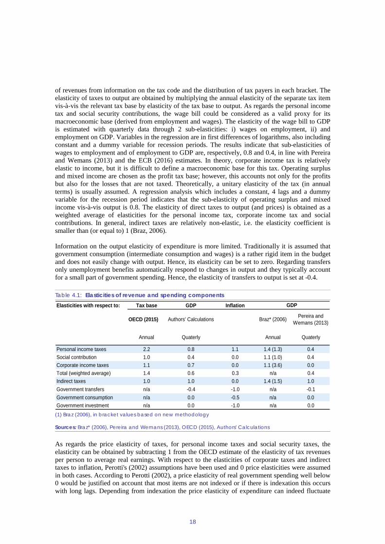
of revenues from information on the tax code and the distribution of tax payers in each bracket. The elasticity of taxes to output are obtained by multiplying the annual elasticity of the separate tax item vis-à-vis the relevant tax base by elasticity of the tax base to output. As regards the personal income tax and social security contributions, the wage bill could be considered as a valid proxy for its macroeconomic base (derived from employment and wages). The elasticity of the wage bill to GDP is estimated with quarterly data through 2 sub-elasticities: i) wages on employment, ii) and employment on GDP. Variables in the regression are in first differences of logarithms, also including constant and a dummy variable for recession periods. The results indicate that sub-elasticities of wages to employment and of employment to GDP are, respectively, 0.8 and 0.4, in line with Pereira and Wemans (2013) and the ECB (2016) estimates. In theory, corporate income tax is relatively elastic to income, but it is difficult to define a macroeconomic base for this tax. Operating surplus and mixed income are chosen as the profit tax base; however, this accounts not only for the profits but also for the losses that are not taxed. Theoretically, a unitary elasticity of the tax (in annual terms) is usually assumed. A regression analysis which includes a constant, 4 lags and a dummy variable for the recession period indicates that the sub-elasticity of operating surplus and mixed income vis-à-vis output is 0.8. The elasticity of direct taxes to output (and prices) is obtained as a weighted average of elasticities for the personal income tax, corporate income tax and social contributions. In general, indirect taxes are relatively non-elastic, i.e. the elasticity coefficient is smaller than (or equal to) 1 (Braz, 2006).

Information on the output elasticity of expenditure is more limited. Traditionally it is assumed that government consumption (intermediate consumption and wages) is a rather rigid item in the budget and does not easily change with output. Hence, its elasticity can be set to zero. Regarding transfers only unemployment benefits automatically respond to changes in output and they typically account for a small part of government spending. Hence, the elasticity of transfers to output is set at -0.4.

Table 4.1: Elasticities of revenue and spending components

(1) Braz (2006), in bracket values based on new methodology Sources: Braz* (2006), Pereira and Wemans (2013), OECD (2015), Authors' Calculations

As regards the price elasticity of taxes, for personal income taxes and social security taxes, the elasticity can be obtained by subtracting 1 from the OECD estimate of the elasticity of tax revenues per person to average real earnings. With respect to the elasticities of corporate taxes and indirect taxes to inflation, Perotti's (2002) assumptions have been used and 0 price elasticities were assumed in both cases. According to Perotti (2002), a price elasticity of real government spending well below 0 would be justified on account that most items are not indexed or if there is indexation this occurs with long lags. Depending from indexation the price elasticity of expenditure can indeed fluctuate

Elasticities with respect to: Tax base GDP Inflation

OECD (2015) Authors' Calculations Braz* (2006) Pereira and Wemans (2013)

Annual Quaterly Annual Quaterly

Personal income taxes 2.2 0.8 1.1 1.4 (1.3) 0.4Social contribution 1.0 0.4 0.0 1.1 (1.0) 0.4Corporate income taxes 1.1 0.7 0.0 1.1 (3.6) 0.0Total (weighted average) 1.4 0.6 0.3 n/a 0.4Indirect taxes 1.0 1.0 0.0 1.4 (1.5) 1.0Government transfers n/a -0.4 -1.0 n/a -0.1Government consumption n/a 0.0 -0.5 n/a 0.0Government investment n/a 0.0 -1.0 n/a 0.0

GDP

19

between 0 and -1. If expenditures are 'fixed in nominal terms this means no indexation and the elasticity would be around -1 as real expenditure declines when prices increase. In the case of indexed spending items, like drugs in the health service, then the elasticity can be around 0. To this end, an elasticity of -0.5 has been considered for government consumption. Similarly, the indexation of transfer programmes occurs usually with substantial lags, which would justify negative price elasticity for real government transfers. In Portugal only pension expenditure is due to automatic indexations but still taking into account the previous year's inflation (OECD, 2013), thus taking into account the indexation policy and share of pension in the total transfers, the price elasticity of government transfers was set to -1 (see Table 4.1).

Such adjustments done through the elasticities can help isolate the cyclical from the discretionary component of the fiscal variable. The analysis of the multipliers then uses the discretionary component. The elasticities used for each tax category and some spending items compare well with those estimated by Pereira and Wemans (2013) apart from the elasticity of the corporate income tax that in Pereira and Wemans (2013) is set to zero. According to .Pereira and Wemans (2013) the revenue from this tax in Portugal is primarily related to previous years’ profits, they posit a zero elasticity of the tax to quarterly GDP. However, the latter approach bears some limitations as only a part of the payments relates to the previous year. Given to its small weight, corporate tax revenue plays a little impact in the average elasticities for the overall capital and labour taxes. Income taxes and social contributions elasticities are here on the higher side if compared with Pereira and Wemans (2013), but mainly due to lower annual elasticities vis-à-vis tax bases (OECD recalculated new elasticities in 2015). The significantly higher Braz (2006) elasticities is explained by the use of annual data as, annual elasticities tend to be higher than quarterly.

5. EMPIRICAL RESULTS

21

A VAR of order 4 was selected for the SVAR identification for the period 1995-2017. The lag length was selected according to selection criteria tests for lags (see Table 2 in the annex), in particular the Akaike criterion whose results seemed to be more consistent with what performed by the literature. The reduced form residuals of the standard VAR are close to being Gaussian white noise disturbances, though correlated across the equations of endogenous variables. As the benchmark model, the one with the intercept vector was selected. The trend components were also tried but the former was shown to perform better. The analysis is made by investigating the orthogonal impulse-response functions of the estimated models. The focus is on the responses of macroeconomic variables: real output, HICP inflation and the interest rate of ten-year government bonds. The responses to a one-time shock to fiscal variables are presented in Table 5.1 and Graphs 1-3 in the Annex. As benchmark a shock of a 1% change to fiscal variables was applied and the two-standard deviation confidence bands have been obtained by Monte Carlo simulations with 1000 replications (5% significance level).(5) For many impulse responses, estimates point to weak statistical significance. This is largely due to the small dimension of the sample, a factor behind the common imprecision of impulse-response functions in VAR models and the consequently wide confidence intervals of the VAR estimates. Since the purpose of this paper is to analyse the impact of fiscal policy on GDP, output multipliers were calculated and are reported in Table 5.2. While Table 5.1 shows the reaction of GDP, inflation and interest rates to a 1% change in fiscal variables, Table 5.2 reports the reaction of GDP to a 1 euro change in fiscal variables.

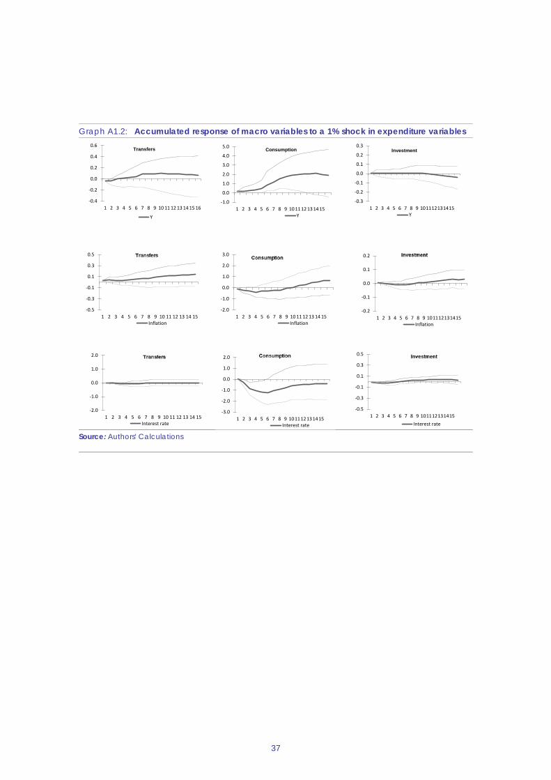
Output Overall we find positive small output responses to taxes, large and positive responses to government consumption, negligible responses to investment and a negative but small response to changes in public transfers. With the exception for government consumption, the impact is short-lived (maximum two quarters) and quite small (largely below unity). More specifically, the impact of an increase in direct taxes on GDP is negative, relatively small (below unity) and significant over only two quarters. The impulse response coefficient is initially 0.02 percent and slowly increases to 0.06 at quarter 6, suggesting a contained and sluggish impact of direct taxes on Portuguese GDP over the estimation horizon (Table 5.1). The effect of indirect taxes on GDP remains small throughout the estimation horizon and is unstable, as it starts as positive and significant at 0.02 in the first quarter to then turn to negative, insignificant and at around 0.01 at quarter 6. Such weak and unstable coefficient for indirect taxes in Portugal could be justified based on the relatively inelastic consumption patterns in the country, as reported by Pereira and Roca-Sagalés (2011). Output responses to shocks in government consumption are on the contrary quite large, significant and positive throughout the entire impulse response horizon (6). The impulse response coefficient increases substantially from 0.18 in the first quarter to 0.84 in the last quarter, showing high persistence of government consumption shocks on GDP. With public wages as the largest component of government consumption, such coefficient might support the argument of disposable income as an important channel for fiscal policy. However, the different reaction of output to changes in taxes and changes in wages may reflect differences in propensity to consume between those economic agents mostly affected by tax changes and those mostly affected by expenditure changes.

(5) Extending the number of bootstraps Montecarlo simulations to 10000 did not change the results. (6) Conclusions on the significance are based on the confidence bounds obtained from Monte Carlo simulations. If

the confidence interval includes 0, a response to the impulse can be considered as statistically insignificant.

22

Results from the SVAR on public investment(7) point to an almost zero output response to investment shocks. This could be primarily due to the fact that investment projects have a longer-term impact than the one of six quarters examined in this study. In addition, a specific explanation for the case of Portugal, is that most public investment in the country is done through public-private –partnerships (PPPs) which historically were not recorded in public investment. In general, the public investment conducted through PPPs tends to have particularly high multipliers (motorways, hospitals) compared to investments implemented by the general government.

Table 5.1: Impulse response coefficients to a 1% shock

(1)*represents 5% significance level Source: Authors' Calculations

Results from the SVAR for public transfers show an initially significant and small output response with a puzzling negative sign, at least for the first two quarters. Such result could be explained by the fact that a large component of this spending item in the form of transfers to companies may not have an immediate impact on aggregate demand, and actually the coefficient could potentially mask some reverse causality or omitted variable bias, in the case of a negative GDP shock which by affecting companies would call for government transfers.

The first year cumulative multipliers provide a better picture on the size of the impact of fiscal shocks on GDP (Table 5.2). Fiscal multipliers are calculated based on the Blanchard and Perotti's (7) Public investment here and transfers in the following paragraph have replaced government consumption in the

estimation.

Quarters 1 2 4 6GDP

Labour and capital taxes -0.02* -0.02* -0.02 -0.05Indirect tax 0.02* 0.02* -0.01 -0.01Government consumption 0.18* 0.21* 0.32* 0.84*Government investment 0.00* 0.00 0.00 0.00Government transfers -0.04* -0.04* 0.01 0.04

HICPLabour and capital taxes 0.01* 0.04* 0.06* 0.08*Indirect tax 0.02* 0.03* 0.04* 0.04Government consumption -0.11* -0.22* -0.42 -0.31Government investment 0.00* 0.00* -0.01* -0.01Government transfers 0.02* 0.03 0.02 0.05

Interest rateLabour and capital taxes 0.03* 0.06* 0.06 0.04Indirect tax -0.02* -0.04* -0.02 0.00Government consumption 0.01* -0.29* -1.02* -1.23Government investment -0.01* -0.02* -0.02* 0.00Government transfers -0.02* -0.03* -0.09 -0.01

23

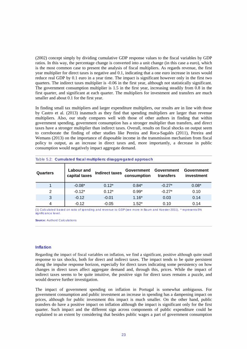
(2002) concept simply by dividing cumulative GDP response values to the fiscal variables by GDP ratios. In this way, the percentage change is converted into a unit change (in this case a euro), which is the most common case to present the analysis of fiscal multipliers. As regards revenue, the first year multiplier for direct taxes is negative and 0.1, indicating that a one euro increase in taxes would reduce real GDP by 0.1 euro in a year time. The impact is significant however only in the first two quarters. The indirect taxes multiplier is -0.06 in the first year, although not statistically significant. The government consumption multiplier is 1.5 in the first year, increasing steadily from 0.8 in the first quarter, and significant at each quarter. The multipliers for investment and transfers are much smaller and about 0.1 for the first year.

In finding small tax multipliers and larger expenditure multipliers, our results are in line with those by Castro et al. (2013) inasmuch as they find that spending multipliers are larger than revenue multipliers. Also, our study compares well with those of other authors in finding that within government spending, government consumption has a stronger multiplier than transfers, and direct taxes have a stronger multiplier than indirect taxes. Overall, results on fiscal shocks on output seem to corroborate the finding of other studies like Pereira and Roca-Sagalés (2011), Pereira and Wemans (2013) on the importance of disposable income in the transmission mechanism from fiscal policy to output, as an increase in direct taxes and, more importantly, a decrease in public consumption would negatively impact aggregate demand.

Table 5.2: Cumulated fiscal multipliers: disaggregated approach

(1) Calculated based on ratio of spending and revenue to GDP (see more in Baum and Koester 2011), * represents 5% significance level. Source: Authors' Calculations

Inflation Regarding the impact of fiscal variables on inflation, we find a significant, positive although quite small response to tax shocks, both for direct and indirect taxes. The impact tends to be quite persistent along the impulse response horizon, especially for direct taxes indicating some persistency on how changes in direct taxes affect aggregate demand and, through this, prices. While the impact of indirect taxes seems to be quite intuitive, the positive sign for direct taxes remains a puzzle, and would deserve further investigation.

The impact of government spending on inflation in Portugal is somewhat ambiguous. For government consumption and public investment an increase in spending has a dampening impact on prices, although for public investment this impact is much smaller. On the other hand, public transfers do have a positive impact on inflation although the impact is significant only for the first quarter. Such impact and the different sign across components of public expenditure could be explained to an extent by considering that besides public wages a part of government consumption

Quarters Labour and capital taxes Indirect taxes Government

consumptionGovernment

transfersGovernment investment

1 -0.08* 0.12* 0.84* -0.27* 0.08*2 -0.12* 0.12* 0.99* -0.27* 0.103 -0.12 -0.01 1.16* 0.03 0.144 -0.12 -0.05 1.52* 0.10 0.14

24

(and investment) is channelled to non-market production (like education, police, justice, army…) or to production with regulated prices (health care, administrative fees…). Thereby, the negative coefficient could reflect some crowding out of private demand, which would then decline as government consumption increases, hence reducing pressure on prices. On the contrary, as transfers are more likely channelled through market production (both transfers to companies and households) then inflationary pressure would mount. Combining these results with those of the output responses, however, seems to suggest that the output increases triggered by a higher wage bill, counterintuitively, would not be reflected into higher prices. Hence, we examine whether, as often claimed by the literature (Perotti 2002), such result could be sensitive to the choice of the elasticity used for spending. Overall, the interpretation of inflation responses to fiscal shocks remains inconclusive and as such in line with Henry et al. (2004), for whom the relationship between government demand and prices remains an open question as it is difficult to assess whether demand or supply channels would prevail.

Interest rate Portuguese interest rates show some negative reaction to shocks in government expenditure, especially for public investment and from Q2 for government consumption. Interest rate responses to tax shocks are more ambiguous as they are positive for direct taxes and negative for indirect taxes. We broadly find then that a deficit increase is followed by decreasing interest rates, which invalidates the argument of bond vigilantes, whereby investors are ready to buy or sell bonds according to fiscal policy changes. The direction of the impact is consistent with what found by Perotti (2002) for some EU countries, and might reflect a fiscal policy tuned to the ECB monetary policy, or, as we are looking at real interest rates, it can capture the impact of higher inflation on the real rates.

Robustness checks We performed a variety of robustness checks for our baseline SVAR model. First of all, we check whether the ordering of the variables in the restrictions might alter the results. Hence, we rerun the model by inverting the ordering which now goes from direct taxes to expenditure (T2, T1 and G). As reported in Table 5.3, the change in ordering does not affect our estimates, with only very few values (in bold) different from the baseline but for the second decimal. An explanation for this could be that as expressed in Perotti (2002), the correlation between the different reduced forms fiscal shocks is relatively low.

25

Table 5.3: Impulse response coefficients with inverted order

*represents 5% significance level Source: Authors' Calculations

Second we test to see whether the estimates are sensitive to the period selected. The period under examination (1995-2017) features several major events for the Portuguese economy which might in fact affect the estimation in case they produced a structural break in the series. To address the effect of potential structural breaks, which could have occurred in particular during the financial crisis, we performed the same analysis for the sub-set 1995-2008.(8) For the sub-set, a two-lag equation system was selected, instead of 4, as better performing for the estimation. Table 5.4 shows small tax multipliers, positive government consumption and investment multipliers, and negative transfer multipliers. These results are broadly consistent with the results for 1995-2017 as far as the signs are concerned, however, they tend to be less significant. Also, government consumption has a larger impact than estimated for the entire period. This could possibly be because of serious debt sustainability issues after the outbreak of the crisis in Portugal, which largely limited fiscal expansions.

(8) Due to data limitation, it was not possible to look separately at other important periods, as opposed to truncating

the series in 2008. An important structural break for Portugal could have been for example the adoption of the Euro in 1999, which is followed by a rapid build-up of Portuguese debt, starting in particular in 2001.

Quarters 1 2 4 6GDP

Labour and capital taxes -0.02* -0.02* -0.02 -0.06Indirect tax 0.01* 0.02* -0.01 -0.01Government consumption 0.17* 0.20* 0.31* 0.83*

HICPLabour and capital taxes 0.00* 0.03* 0.06* 0.07*Indirect tax 0.02* 0.03* 0.04* 0.04Government consumption -0.11* -0.22* -0.42 -0.31

Interest rateLabour and capital taxes 0.03* 0.06* 0.06 0.04Indirect tax -0.02* -0.04* -0.02 0.00Government consumption 0.01* -0.30* -1.03* -1.23

26

Table 5.4: Cumulated fiscal multipliers: 1995-2008

(1) * represents 5% significance level Source: Authors' Calculations

Third, we test to see whether the estimates are sensitive to the period selected from 1999 to 2017 as for quarterly data social security contributions have been extrapolated from OECD annual data for the period 1995-99. As reported in Table 5.5, the change in sample to 1999-2017 affects coefficients for directs taxes and government consumptions, the magnitude of impulse response increased for the direct taxes and decreased for government consumptions in the short-run, while for other variables it remained broadly in line with the baseline model.

Table 5.5: Impulse response coefficients: 1999-2017

(1) Impulse response coefficients: 1999-201 Source: Authors' Calculations

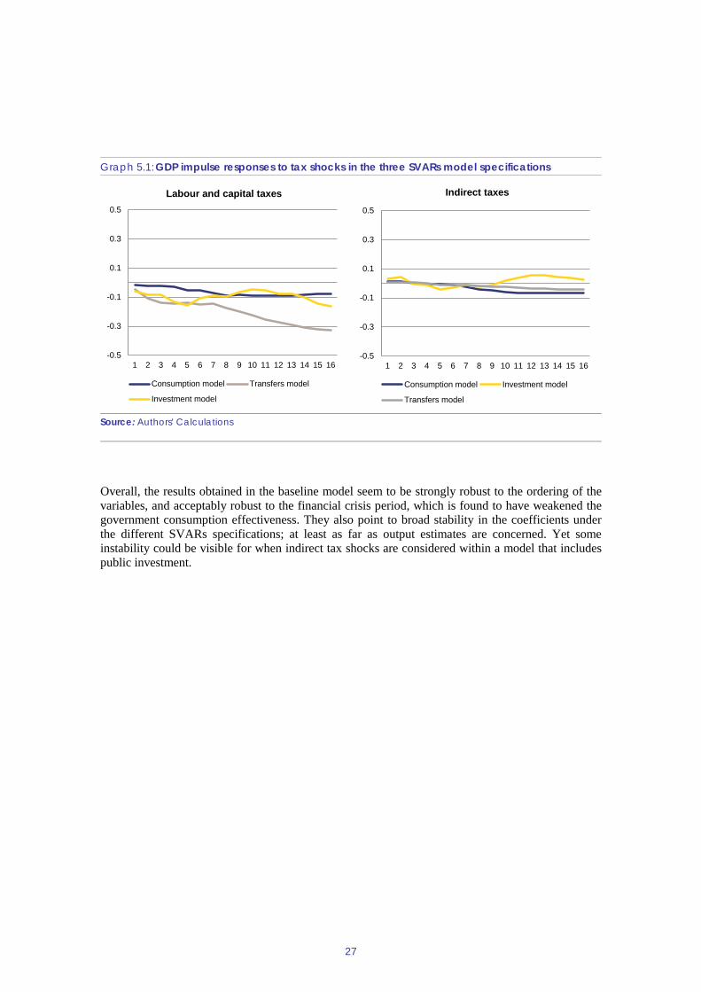
Finally, we look at the GDP impulse response charts to revenue shocks (direct and indirect taxes) obtained in the three SVARs estimation, namely the estimation with government consumption, the one with public investment and the one with transfers. Graph 5.1 here below shows no substantial difference in the behaviour of GDP impulse responses to direct tax shocks within the three models, as coefficients fluctuate between 0 and -0.2. More fluctuation is instead visible for the impulse responses to indirect tax shocks, in particular in the case of the investment model, as the coefficient is unstable in the sign.

Quarters Labour and capital taxes Indirect taxes Government

consumptionGovernment

transfersGovernment investment

1 -0.13* 0.09* 2.42* -0.64* 0.10*2 0.09 0.09 4.94 -0.52 0.203 0.01 0.10 9.29 -0.81 0.144 -0.09 0.27 15.82 -0.91 0.14

Quarters 1 2 4 6GDP

Labour and capital taxes -0.10* -0.13* -1.80 -0.18Indirect tax 0.01* 0.00* 0.01 0.03Government consumption 0.22* 0.18* 0.40 1.36

HICPLabour and capital taxes 0.01* 0.00* 0.00* -0.02*Indirect tax 0.02* 0.03* 0.04* 0.04Government consumption -0.13* -1.02* -1.02 -0.74

Interest rateLabour and capital taxes 0.08* 0.13* 0.14 0.10Indirect tax -0.02* -0.06* -0.08 -0.11Government consumption -0.04* -0.43 -1.13* -1.19

27

Overall, the results obtained in the baseline model seem to be strongly robust to the ordering of the variables, and acceptably robust to the financial crisis period, which is found to have weakened the government consumption effectiveness. They also point to broad stability in the coefficients under the different SVARs specifications; at least as far as output estimates are concerned. Yet some instability could be visible for when indirect tax shocks are considered within a model that includes public investment.

Graph 5.1: GDP impulse responses to tax shocks in the three SVARs model specifications

Source: Authors' Calculations

-0.5

-0.3

-0.1

0.1

0.3

0.5

1 2 3 4 5 6 7 8 9 10 11 12 13 14 15 16

Labour and capital taxes

Consumption model Transfers model

Investment model

-0.5

-0.3

-0.1

0.1

0.3

0.5

1 2 3 4 5 6 7 8 9 10 11 12 13 14 15 16

Indirect taxes

Consumption model Investment model

Transfers model

6. CONCLUSION

29

This paper sheds some light on the implications of fiscal policy on the Portuguese economy. This is done by using a restricted VAR model, which has become one of the most popular tool for investigating the effects of fiscal and monetary policy on growth. In the case of Portugal, empirical evidence on the effects of fiscal policy on macro variables is still limited and mostly concentrated on GDP multipliers. In addition to growth, the focus of this study encompasses the implications of fiscal policy on inflation and on long-term interest rates.

The analysis provides some interesting results that could be useful for policy making. Regarding the impact of fiscal policy shocks on growth, our findings do not depart much from the relevant literature. We indeed find that disposable income is an important channel for the transmission mechanism from fiscal policy to growth. Government consumption triggers relatively large and persistent positive output responses in Portugal, while the short-term impact of transfers and investment is small. Tax revenue has a significant and negative impact on output through direct taxes but the impact is small and short-lived. Indirect taxes display a pass-through on inflation that is persistent over time. We also find that the government consumption multiplier was larger before the financial crisis, pointing to some inefficiency in fiscal policy transmission channels during and after the crisis. The estimation results on the way inflation reacts to fiscal shocks would benefit from further analysis, as in particular the negative impact on inflation coming from government consumption hardly squares with the results from the output multiplier analysis.

Finally, the analysis presents the usual caveats associated with the use of restricted VARs. First, as noted the relatively small size of the sample affects the statistical significance of the results. In most cases the impulse response results are significant only over the short run. Second, the specification used for the structural VAR does not allow capturing structural breaks, besides the one of the financial crisis, accounted for in the robustness check part. As mentioned, other shocks could have occurred in the early 2000s with the introduction of the euro and may represent some structural breaks. Also, the specification used does not allow distinguishing for state-dependence. More research would be warranted in this direction as indeed the period under consideration displays important changes in the economic development of Portugal.

REFERENCES

31

Afonso A., Sousa R. M. (2011), "The macroeconomic effects of fiscal policy in Portugal: a Bayesian SVAR analysis", Portuguese Journal of Economics, vol. 10, pp. 61-82.

Auerbach, A.J., Gorodnichenko, Y. (2012), "Fiscal Multipliers in Recession and Expansion", in Fiscal Policy after the Financial Crisis, ed. by A. Alesina and F. Giavazzi (Chicago: University of Chicago Press).

Batini, N., Eyraud, L., Forni, L., Weber, A. (2014), Fiscal Multipliers: Size, Determinants, and Use in Macroeconomic Projections, IMF, Fiscal Affairs Department.

Baum, A., Koester, G. D. (2011), "The impact of fiscal policy on economic activity over the business cycle – evidence from a threshold VAR analysis", Deutsche Bundesbank, Discussion Paper Series 1: Economic Studies No 03/2011.

Biau O., Girard E. (2005), “Politique budgétaire et dynamique économique en France: l'approche VAR structurel”, Revue économique, Vol. 56, pp. 755-764

Blanchard, O. J., Perotti, R. (2002), “An Empirical Characterization of the Dynamic Effects of Changes in Government Spending and Taxes on Output”, The Quarterly Journal of Economics, 117, pp. 1329-1368.

Braz C R. (2006), "The Calculation of Cyclically Adjusted Balances at Banco de Portugal: an update", Banco de Portugal Economic Bulletin, Winter 2006.

Canova F., Pappa E. (2002), "Price Dispersions in Monetary Unions: the Role of Fiscal Shocks", paper presented at the CEPR- INSEAD conference on "Political, Institutional and Economic Determinants of Fiscal Policy", Fontainebleau, 7-10 November.

Castro G., Felix R. M., Julio P., Maria J. R. (2013), "Fiscal Multipliers in a Small Euro Area Economy: How big can they get in crisis times?", Banco de Portugal Working Paper 11/2013.

Christiano L., Eichenbaum M., Rebelo S. (2011) “When Is the Government Spending Multiplier Large?”, Journal of Political Economy, 119(1): 78–121.

Cléaud G., Lemoine M., Pionnier P.-A. (2013), “Which size and evolution of the government expenditure multiplier in France (1980-2010)?” mimeo.

Coenen G., Erceg C. J., Freedman C., Furceri D., Kumhof M., Lalonde R., Laxton D., Lindé J., Mourougane A., Muir D., Mursula S., de Resende C., Roberts J., Roeger W., Snudden S., Trabandt M., in't Veld J. (2012), "Effects of Fiscal Stimulus in Structural Models", American Economic Journal: Macroeconomics, 4 (1): 22-68.

De Castro F. (2006), “The macroeconomic effects of fiscal policy in Spain”, Applied Economics, 38, pp. 913-924.

De Castro F., Fernandez L. (2013), “The Effects of Fiscal Shocks on the Exchange Rate in Spain”, The Economic and Social Review, Vol 44, n. 2, pp. 151-180.

De Castro F., Hernandez de Cos P. (2008), “The Economic Effects of Fiscal Policy: The Case of Spain”, Journal of Macroeconomics, Vol. 30, pp. 1005-1028.

32

Dell'Erba S., Sola S. (2011), "Expected Fiscal Policy and Interest Rates in Open Economy", The Graduate Institute of International and Development Studies (IHEID) Working Paper, 07-2011.

ECB (2016), Economic Bulletin, Issue 6 / 2016.

Fatás A., Mihov I. (2001), "The Effects of Fiscal Policy on Consumption and Employment: Theory and Evidence", mimeo, INSEAD.

Favero C., Giavazzi F. (2012), "Measuring Tax Multipliers: The Narrative Method in Fiscal VARs", American Economic Journal: Economic Policy, Vol. 4, n. 2, pp. 69–94.

Gale W., Orszag P. (2002), "The economic effects of long term fiscal discipline", Tax Policy Center Discussion Paper, December.

Giordano R. S., Momigliano S., Neri S., Perotti R. (2007), "The effects of fiscal policy in Italy: Evidence from a VAR model", European Journal of Political Economy n. 23, pp. 707–733.

Guajardo J., Leigh D., Pescatori A. (2014), "Expansionary Austerity: International Evidence", Journal of the European Economic Association, Vol. 12, n. 4, pp. 949-968.

Henry J., Hernandez de Cos P., Momigliano S. (2004), "The short-term Impact of Government Budgets on Prices. Evidence from Macroeconometric Models", European Central Bank Working Paper Series, n. 396.

Heppke-Falk K. H., Tenhofen J., Wolff G. B. (2006), "The macroeconomic effects of exogenous fiscal policy shocks in Germany: a disaggregated SVAR analysis", Deutsche Bundesbank Discussion Paper Series 1, n 41.

Ilzetzki E., Mendoza E. G., Végh C. A. (2011), "How big (small?) are fiscal multipliers?", IMF Working Paper 11/52.

Krugman P. (2012), "The Simple Analytics of Invisible Bond Vigilantes," New York Times, November 9 2012, available at: https://krugman.blogs.nytimes.com/2012/11/09/the-simple-analytics-of-invisible-bond-vigilantes-wonkish/.

Laubach T. (2011), "Fiscal Policy and Interest Rates: The Role of Sovereign Default Risk", NBER International Seminar on Macroeconomics, University of Chicago Press, Vol. 7, n. 1, pp. 7-30.

Lütkepohl H. (2005), New Introduction to Multiple Time Series Analysis, Berlin, New York: Springer.

Marcellino M. (2002), "Markups and the Business Cycles: Real Facts and a Monetary Myth", Federal Reserve Bank of Minneapolis Quarterly Review, August.

Mertens R., Ravn M. O. (2012), "A Reconciliation of SVAR and Narrative Estimates of Tax Multipliers", CEPR Discussion Paper 8973 (London: Center for Economic Policy Research).

Mineshima A., Poplawski-Ribeiro M., Weber A. (2014), "Fiscal Multipliers", in Post-Crisis Fiscal Policy, eds. by C. Cottarelli, P. Gerson and A. Senhadji (Cambridge: MIT Press).

Mountford A., Uhlig H. (2009), "What Are the Effects of Fiscal Policy Shocks?", Journal of Applied Econometrics, Vol. 24, n.6, pp. 960-992.

33

OECD (2013), "Pensions at a Glance 2013: Portugal", http://www.oecd.org/els/public-pensions/PAG2013-profile-Portugal.pdf

Pereira A. M., Roca-Sagalés O. (2011),"Long-term effects of fiscal policies in Portugal", Journal of Economic Studies, Vol. 38, n. 1, pp. 114 – 127.

Pereira M. C., Wemans L. (2013), "Output Effects of Fiscal Policy in Portugal: a Structural Var Approach", Banco de Portugal Economic Bulletin, Spring 2013.

Perotti R. (2002), "Estimating the Effects of Fiscal Policy in OECD countries", ECB working paper 168.

Perotti R. (2004), "Estimating the effects of fiscal policy in OECD countries", Proceedings of Federal Reserve Bank of San Francisco.

Poirier R. (2014), "Fiscal Multipliers in Portugal Using a Threshold Approach", NOVA School of Business and Economics, mimeo.

Ramey V. (2011), "Identifying Government Spending Shocks: It's All in the Timing", Quarterly Journal of Economics, Vol. 126, n. 1, pp. 1-50.

Romer, C.D, Romer D. H. (2010), "The Macroeconomic Effects of Tax Changes: Estimates Based on a New Measure of Fiscal shocks", American Economic Review, Vol. 100, pp. 763-801.

Spilimbergo A., Symansky S., Schindler M. (2009), "Fiscal Multipliers", IMF Staff Position Note 09/11 (Washington: International Monetary Fund).

Woodford M., (2011), "Simple Analytics of the Government Expenditure Multiplier", American Economic Journal: Macroeconomics, Vol.3, n. 1, pp. 1-35.

ANNEX 1

35

Table A1.1: Unit root test results

* and ** represent the rejection of the null hypothesis at significance levels of 1% and 5% respectively. Source: Authors' Calculations

Table A1.2: Lag determination test results

(1) *Information criteria: AIC for Akaike; HQ for Hannan-Quinn; SC for Schwarz; FPE for forecast prediction error. ** represents the best lag length suggested by each criterion Source: Authors' Calculations

ADF testtrend+const. const. none const. none

Real GDP -2.42 -2.72 1.39 -3.037* -3.45HICP -0.81 -1.53 2.36 -0.75 -1.99 5.57Long term nominal interest rate -1.23 -3.33** -2.08** -2.57 -2.64 -1.95*Real direct taxes -2.88 -1.73 1.21 -8.47** -4.45** 0.76Real social contributions -1.61 -2.84* 2.44 -1.65 -2.65 2.04Real indirect taxes -2.21 -2.09 1.51 -3.23** -2.32 0.81Real public consumption -1.25 -1.65 -1.71 -1.18 -2.96* 1.48**Real public transfers -2.88 -1.73 1.21 -4.45** -8.47** 0.76Real public investment -5.05** -1.8 -1.19 -3.90** -2.39 -0.98

PP test

trend+const.

Criteria* 1 2 3 4 5 6Government consumption modelAIC 2.42 2.19 2.39 1.929** 1.96 2.06HQ 2.903** 3.09 3.71 3.66 4.11 4.62SC 3.625** 4.43 5.67 6.24 7.30 8.44FPE 11.25 9.09 11.48 7.662** 8.75 11.35Government investment modelAIC(n) 5.73 5.55 5.77 5.483** 5.54 5.40HQ(n) 6.219** 6.45 7.09 7.22 7.69 7.96SC(n) 6.939** 7.79 9.04 9.79 10.89 11.78FPE(n) 309.50 261.109** 335.06 267.87 315.91 320.76Government transfers modelAIC(n) 10.99 10.98 10.86 10.266** 10.66 10.45HQ(n) 11.568** 12.06 12.44 12.34 13.23 13.52SC(n) 12.479** 13.75 14.91 15.60 17.27 18.34FPE(n) 59485.06 61498.42 60430.86 41278.99** 89437.80 140488.18

36

Graph A1.1: Accumulated response of macro variables to a 1% shock in tax variables

Source: Authors' Calculations

-0.3

-0.2

-0.1

0.0

0.1

0.2

0.3

1 2 3 4 5 6 7 8 9 10 11 12 13 14 15

Indirect taxes

Y

-0.3

-0.2

-0.1

0.0

0.1

0.2

0.3

1 2 3 4 5 6 7 8 9 10 11 12 13 14 15

Labour and capital taxes

Inflation

-0.3

-0.2

-0.1

0.0

0.1

0.2

0.3

1 2 3 4 5 6 7 8 9 10 11 12 13 14 15

Labour and capital taxes

Interest rate

-0.3

-0.2

-0.1

0.0

0.1

0.2

0.3

1 2 3 4 5 6 7 8 9 10 11 12 13 14 15

Indirect taxes

Interest rate

-0.3

-0.2

-0.1

0.0

0.1

0.2

0.3

1 2 3 4 5 6 7 8 9 10 11 12 13 14 15

Indirect taxes

Inflation

-0.3-0.2-0.10.00.10.20.3

1 2 3 4 5 6 7 8 9 10 11 12 13 14 15 16

Labour and capital taxes

Y

37

Graph A1.2: Accumulated response of macro variables to a 1% shock in expenditure variables

Source: Authors' Calculations

-1.0

0.0

1.0

2.0

3.0

4.0

5.0

1 2 3 4 5 6 7 8 9 10 11 12 13 14 15

Consumption

Y

-2.0

-1.0

0.0

1.0

2.0

3.0

1 2 3 4 5 6 7 8 9 10 11 12 13 14 15Inflation

-3.0

-2.0

-1.0

0.0

1.0

2.0

1 2 3 4 5 6 7 8 9 101112131415Interest rate

-0.4

-0.2

0.0

0.2

0.4

0.6

1 2 3 4 5 6 7 8 9 10 11 12 13 14 15 16

Transfers

Y

-2.0

-1.0

0.0

1.0

2.0

1 2 3 4 5 6 7 8 9 10 11 12 13 14 15Interest rate

-0.3

-0.2

-0.1

0.0

0.1

0.2

0.3

1 2 3 4 5 6 7 8 9 101112131415

Investment

Y

-0.5

-0.3

-0.1

0.1

0.3

0.5

1 2 3 4 5 6 7 8 9 101112131415Interest rate

-0.5

-0.3

-0.1

0.1

0.3

0.5

1 2 3 4 5 6 7 8 9 10 11 12 13 14 15Inflation

-0.2

-0.1

0.0

0.1

0.2

1 2 3 4 5 6 7 8 9 101112131415Inflation

EUROPEAN ECONOMY DISCUSSION PAPERS European Economy Discussion Papers can be accessed and downloaded free of charge from the following address: https://ec.europa.eu/info/publications/economic-and-financial-affairs-publications_en?field_eurovoc_taxonomy_target_id_selective=All&field_core_nal_countries_tid_selective=All&field_core_date_published_value[value][year]=All&field_core_tags_tid_i18n=22617. Titles published before July 2015 under the Economic Papers series can be accessed and downloaded free of charge from: http://ec.europa.eu/economy_finance/publications/economic_paper/index_en.htm.

GETTING IN TOUCH WITH THE EU In person All over the European Union there are hundreds of Europe Direct Information Centres. You can find the address of the centre nearest you at: http://europa.eu/contact. On the phone or by e-mail Europe Direct is a service that answers your questions about the European Union. You can contact this service:

• by freephone: 00 800 6 7 8 9 10 11 (certain operators may charge for these calls),

• at the following standard number: +32 22999696 or • by electronic mail via: http://europa.eu/contact.

FINDING INFORMATION ABOUT THE EU Online Information about the European Union in all the official languages of the EU is available on the Europa website at: http://europa.eu. EU Publications You can download or order free and priced EU publications from EU Bookshop at: http://publications.europa.eu/bookshop. Multiple copies of free publications may be obtained by contacting Europe Direct or your local information centre (see http://europa.eu/contact). EU law and related documents For access to legal information from the EU, including all EU law since 1951 in all the official language versions, go to EUR-Lex at: http://eur-lex.europa.eu. Open data from the EU The EU Open Data Portal (http://data.europa.eu/euodp/en/data) provides access to datasets from the EU. Data can be downloaded and reused for free, both for commercial and non-commercial purposes.