Fiscal Stimulus in a Monetary Union:

Evidence from U.S. Regions

Emi Nakamura and Jon Steinsson∗

Columbia University

July 6, 2011

Abstract

We use rich historical data on military procurement spending across U.S. regions to estimate

the effects of government spending in a monetary union. Aggregate military build-ups and

draw-downs have differential effects across regions. We use this variation to estimate an open

economy relative government spending multiplier of approximately 1.5. We develop a framework

for interpreting this estimate and relating it to estimates of closed economy aggregate multipliers.

The closed economy aggregate multiplier is highly sensitive to how strongly aggregate monetary

and tax policy “leans against the wind.” In contrast, our estimate “differences out” these effects

because different regions in the union share a common monetary and tax policy. Our estimate

provides evidence in favor of models in which demand shocks can have large effects on output.

Keywords: Fiscal stimulus, Government Spending, Multiplier, Monetary Union.

JEL Classification: E62, E32

∗We thank Thuy Lan Nguyen for excellent research assistance. We thank Steve Davis, Gauti Eggertsson, JordiGali, Marcelo Moreira, James Stock, Michael Woodford, Pierre Yared, Motohiro Yogo and seminar participants atvarious institutions for helpful comments and conversations.

1 Introduction

The effect of government spending on output is often summarized by a multiplier—the percentage

increase in output that results when government spending is increased by 1% of GDP. There is a

wide range of views about this statistic in the literature. On the one hand, the recent American

Recovery and Reinvestment Act (ARRA)—perhaps the largest fiscal stimulus plan in U.S. history—

was motivated by a relatively high estimate of the multiplier of 1.6 (Romer and Bernstein, 2009).

Other studies argue that the multiplier is substantially less than one and potentially close to zero.

In particular, if the determination of output is dominated by supply-side factors, an increase in

government purchases to a large extent “crowds out” private sector consumption and investment.

The wide range of views on the multiplier arises in part from the difficulty of measuring it.

Changes in government spending are rarely exogenous, leading to a range of estimates depending

on the estimation approach.1 Two main approaches have been used to estimate the multiplier in

the academic literature. The first is to study the output effects of increases in military spending

associated with wars, which are plausibly unrelated to prevailing macroeconomic conditions (Ramey

and Shapiro, 1998; Edelberg, Eichenbaum and Fisher, 1999; Burnside, Eichenbaum and Fisher,

2004; Ramey, 2010; Barro and Redlick, 2011; Fisher and Peters, 2010). The main obstacle faced

by this approach is the relative infrequency of large wars.2 The second main approach used to

identify the multiplier is the structural VAR approach (Blanchard and Perotti, 2002; Perotti, 2007;

Mountford and Uhlig, 2008; Ilzetzki, Mendoza and Vegh, 2010). This approach relies on structural

assumptions about output and fiscal policy dynamics to estimate the multiplier.

The wide range of views on the multiplier also results from a lack of clear predictions in the the-

oretical literature. The government spending multiplier is not a deep structural parameter like the

elasticity of labor supply or the intertemporal elasticity of substitution. Different models, therefore,

differ in their implications about the multiplier depending on what is assumed about preferences,

technology, government policy and various “frictions.” Simple versions of the Neoclassical model

generally imply a small multiplier, typically smaller than 0.5 (see, e.g., Baxter and King, 1993).

1For surveys of the existing evidence, see for example Perotti (2007), Hall (2009), Alesina and Ardagna (2009)and Cogan et al. (2010).

2Most of the evidence from this approach derives from the U.S. experience during WWII and the Korean War, whenchanges in U.S. military spending were largest and most abrupt as a fraction of total output. However, confoundingvariation associated with wartime price controls, patriotism, tax increases, and other macroeconomic shocks remainsources of intense debate regarding the evidence from these episodes. Hall (2009) and Barro and Redlick (2011)emphasize that it is not possible to draw meaningful inference using aggregate data on military spending after 1955because there is insufficient variation in military spending in this period.

1

The multiplier is sensitive to how the spending is financed—smaller if it is financed by distortionary

taxes than lump sum taxes.3 In New Keynesian models, the size of the multiplier depends critically

on the extent to which monetary policy “leans against the wind.” Strongly counter-cyclical mon-

etary policy—such as that commonly estimated for the Volcker-Greenspan period—can generate

quite low multipliers—comparable to those for the Neoclassical model. However, when monetary

policy is less responsive—e.g., at the zero lower bound—the multiplier can exceed two.4 Clearly,

there is no “single” government spending multiplier. All estimates of the government spending

multiplier depend on the policy regime in place. This is likely one contributing factor for the wide

range of empirical estimates of the multiplier discussed above.

We analyze the effects of government spending in a monetary and fiscal union—the United

States. In this setting, we estimate the effect that an increase in government spending in one

region of the union relative to another has on relative output and employment. We refer to this as

the “open economy relative multiplier.” Studying a monetary union has the unique advantage that

the relative monetary policy is pinned down by the fact that the nominal interest rate is common

across the entire region (and the exchange rate is fixed). This implies that increased spending in

one region relative to another cannot lead to tighter monetary policy in that region relative to the

other. Also, federal spending is financed by federal taxes levied in the same way across regions. An

increase in federal spending in one region relative another, therefore, does not increase current or

future tax rates in that region relative to other regions. We show that an important advantage of

being able to precisely specify relative policy across regions is that we can more easily distinguish

between different models of the economy.

We use regional variation in military spending to estimate the multiplier. When national mili-

tary procurement rises by 1 percentage point of GDP, it rises on average by more than 3 percentage

points in defense-intensive states such as California and Connecticut, but by less than one-half of

one percent in defense-insensitive states such as Illinois. This heterogeneity in sensitivity to aggre-

gate military build-ups and draw-downs across regions is the source of variation we use to estimate

the effects of government spending shocks on output, employment and prices.5

3See, e.g., Baxter and King (1993), Ohanian (1997), Corsetti et al., 2009, and Drautzburg and Uhlig (2011).4Intuitively, at the zero lower bound, monetary policy is rendered impotent and a fiscal expansion is particularly

effective since it lowers real interest rates by raising inflation (Eggertsson, 2010; Christiano, Eichenbaum, and Rebelo,2010).

5Since regional variations in military procurement is much larger than aggregate variation, this approach allowsus to overturn the conclusion from the literature that focuses on aggregate data that little can be learned about fiscalmultipliers from the post-1960 data. Data from this period may be more informative about the size of the fiscalmultiplier for “normal times” and “normal purchases” than data from WWII and the Korean war. Several authors

2

A common identifying assumption in the empirical literature on the effects of military spending

is that variation in military spending is exogenous to the U.S. business cycle. Our key identifying

assumption is similar but weaker. We assume that the U.S. does not embark on military buildups—

such as those associated with the Vietnam war and the Soviet invasion of Afghanistan—because

defense oriented states are doing poorly relative to other states. We do not require that idiosyncratic

variations in military procurement—such as the increase in procurement spending in Texas during

the presidency of George W. Bush—are exogenous to local economic conditions.6 By including

time fixed effects, we control for aggregate shocks that affect all states at a particular point in

time—such as changes in distortionary taxes and aggregate monetary policy.

We estimate the “open economy relative multiplier” to be 1.5. In other words, when relative

per-capita government purchases in a region rises by 1% of regional output, relative per-capita

output in that region rises by 1.5%. As we emphasize above, our open economy relative multiplier

differs from a “closed economy aggregate multiplier” one might estimate using aggregate U.S. data.

We develop a theoretical framework to help us interpret our multiplier estimate and assess how it

relates to the closed economy aggregate multiplier for the United States. Our main conclusion is

that our estimate favors models in which demand shocks can have large effects on output. Our

estimate lines up well with the multiplier implied by an open economy New Keynesian model

in which consumption and work are complements.7 Benchmark New Keynesian and Neoclassical

models, however, yield lower open economy relative multipliers.

Our estimate of 1.5 for the open economy relative multiplier is perfectly consistent with much

lower existing estimates of the closed economy aggregate multiplier. A likely reason for the difference

is that the relative monetary policy across regions—fixed relative nominal rate and exchange rate—

is less counter-cyclical than aggregate monetary policy in the U.S.—which raises the real interest

rate substantially in response to inflationary shocks. Our open economy relative multiplier is thus

akin to an aggregate multiplier for a more accommodative monetary policy than the one seen in

the United States.

The logic for why the open economy relative multiplier is higher than the closed economy

suggest that the multiplier may be different for military versus non-military spending, but these findings rely heavilyon the WWII and Korean War experiences when aggregate variation in military spending was largest (e.g., Perotti2007; Auerbach and Gorodnichenko, 2010).

6The allocation of defense spending across U.S. regions is well-known to be influenced by political factors. SeeMintz (1992) for a discussion of political issues related to the allocation of military procurement spending.

7Another potential approach to matching our multiplier estimate would be to consider a model with “hand-to-mouth” consumers as in Gali, Lopez-Salido, and Valles (2007).

3

aggregate multiplier for normal monetary policy is the same as the logic for why the fiscal multiplier

is larger under a fixed exchange rate than a flexible exchange rate in the Mundell-Fleming model.

In fact, we show theoretically that the open economy relative multiplier is exactly the same as the

aggregate multiplier in a small open economy with a fixed exchange rate. This lines up well with

existing empirical evidence. Based on data from 44 countries, Ilzetzki, Mendoza, and Vegh (2010)

estimate a multiplier of 1.5 for countries that operate a fixed exchange rate regime, but a much

lower multiplier for countries operating a flexible exchange rate regime.8

Since the nominal interest rate cannot offset any changes in relative output or inflation across

regions in our setting, one might infer that our setting resembles that of a closed economy in which

the nominal interest rate is at its zero lower bound and New Keynesian models generate large

multipliers. However, this simple intuition ignores a crucial dynamic aspect of price responses in a

monetary union. Since purchasing power parity holds in the long run and the exchange rate is fixed

within the monetary union, any increase in prices in the short run in one region relative to the other

must eventually be reversed in the long run. This implies that even though relative short-term real

interest rates fall in response to government spending shocks in our model, relative long-term real

interest rates don’t (in contrast to the zero lower bound setting). Consumption (and thus output)

is determined by the behavior of the long-term real interest rate via the Euler equation.

An important difference between our open economy relative multiplier and the closed economy

aggregate multiplier is that the regions that receive spending don’t have to pay for it. Could this

perhaps explain the “large” relative multiplier we estimate? To the contrary, both Neoclassical and

New Keynesian business cycle models imply that negative wealth effects raise the fiscal multiplier

(since leisure is a normal good). The absence of a negative wealth effect in our setting should

thus lower the multiplier we estimate relative to a setting in which current and future taxes rise in

proportion to spending. Also, the multiplier that we estimate is not a “windfall” or “manna from

heaven” multiplier. Agents in our setting are getting paid for producing goods and services that

are used for defense of the union as a whole. If labor and product markets are competitive, they

are indifferent at the margin as to whether they get more or less such work.

The theoretical framework we describe may be used to interpret recent and ongoing research

on the effects of other forms of local government spending (Acconcia et al., 2011; Clemens and

Miran, 2010; Cohen et al., 2010; Fishback and Kachanovskaya, 2010; Serrato and Wingender, 2010;

8Kraay (2011) estimates a government spending multiplier or about 0.5 for 29 aid-dependent developing countriesusing variation in World Bank lending.

4

Shoag, 2010; Wilson, 2011). There are some potentially important differences between our study

and these. Some of these studies focus on windfall transfers rather than purchases. Also, military

spending represents government purchases that are much less substitutable for private spending

than most other government purchases. With these caveats in mind, several of these papers also

find large effects of regional government spending which can potentially be explained by similar

factors to those we emphasize in our theoretical model.

Our empirical approach builds on previous work by Davis, Loungani, and Mahidhara (1997),

who study several drivers of regional economic fluctuations, including military procurement.9 Sev-

eral other studies of the impact of defense spending on regional economic fluctuations are surveyed

in Braddon (1995). The most important difference in our empirical methodology relative to these

studies is our use of variation in aggregate military spending in creating instruments to account

for potential endogeneity of local procurement spending. Our work is also related to Canova and

Pappa (2007), who study the price effects of fiscal shocks in a monetary union. Our theoretical

analysis is related to earlier work on monetary and fiscal policy in a monetary union by Benigno

and Benigno (2003) and Gali and Monacelli (2008).

The remainder of the paper is organized as follows. Section 2 described the data we use. Section

3 presents our empirical results. Section 4 presents the model we use to interpret these empirical

results. Section 5 presents our theoretical results. Section 6 concludes.

2 Data

Our main source for military procurement data is the electronic database of DD-350 military

procurement forms available from the US Department of Defense. These forms document military

purchases of everything from repairs of military facilities to the purchase of aircraft carriers. They

cover purchases greater than $10,000 up to 1983 and greater than $25,000 thereafter.10 Relative to

other forms of federal government spending, the geographical distribution of military spending is

remarkably well-documented, perhaps because of the intense political scrutiny surrounding these

purchases. We have used the DD-350 database to compile data on total military procurement by

9Similarly, Hooker and Knetter (1997) estimate the effects of military procurement on subsequent employmentgrowth using a somewhat different specification. Blanchard and Katz (1992) also study the relationship betweenmovements in military procurement variables and subsequent employment growth.

10Purchases reported on DD-350 forms account for 90% of military purchases. Furthermore, our analysis of censusshipment data in section 3 suggests DD-350 purchases account for almost all of the time-series variation in totalmilitary procurement. DD-1057 forms are used to summarize smaller transactions but do not give the identity ofindividual sellers.

5

state and year for 1966-2006.11 DD-350 forms provide detailed information on individual military

procurement contracts, including the amount (and in some cases projected duration) of the contract,

and the location where the majority of the work was performed.12

We have also compiled data on shipments to the government from defense oriented industries.

The source of these data are the Annual Survey of Shipments by Defense-Oriented Industries

conducted by the US Census Bureau from 1963 through 1983. Since there is no electronic version

of these data, we digitized the data from microfilm. This source provides direct evidence on the

timing and location of production associated with military procurement. They allow us to assess

the extent to which some fraction of the prime military contracts reported on DD-350 forms may

have been subcontracted to manufacturers in other states. These data also provide information on

value-added for these manufacturers that we use to calibrate our theoretical model.

Our primary measure of state output is the GDP by state measure constructed by the U.S.

Bureau of Economic Analysis (BEA), which is available since 1963.13 We also make use of anal-

ogous data by major SIC/NAICS grouping.14 We use the BLS payroll survey from the Current

Employment Statistics (CES) program to measure state-level employment. We also present results

for the BEA measure of state employment which is available since 1969. We obtain state population

data from the Census Bureau.15

Finally, to analyze price effects, we construct state and regional inflation measures from several

sources. Before 1995, we rely on state-level inflation series constructed by Marco Del Negro (1998)

for the period 1969-1995 using a combination of BLS regional inflation data and cost of living

estimates from the American Chamber of Commerce Realtors Association (ACCRA).16 After 1995,

we construct state-level price indexes by multiplying a population-weighted average of cost of living

11The electronic military prime contract data file was created in the mid-1960’s and records military prime contractssince 1966. This occurred around the time Robert McNamara was making sweeping changes to the procurementprocess of the U.S. Department of Defense. While aggregate statistics are available before this point, they appearnot to be a reliable source of information on military purchases since large discrepancies arise between actual outlaysand procurement for the earlier period, particularly at the time of the Korean war. See the Department of DefenseGreenbook for aggregate historical series of procurement and outlays.

12These data are for the federal government fiscal year. Since 1976, this has been from October 1st to September30th. Prior to 1976, it was from July 1st to June 30th.

13As an alternative measure of output, we have analyzed BEA State Personal Income data. These data yield similarresults to our baseline measure.

14The data are organized by SIC code before 1997 and NAICS code after 1997. BEA publishes the data for bothsystems in 1997, allowing the growth rate series to be smoothly pasted together.

15Between census years, these data are estimated using a variety of administrative data sources. Since 1970, we arealso able to obtain population by age group, which allows us to adjust our estimates for the working age populationas opposed to the population as a whole.

16See Appendix A of Del Negro (1998) for the details of this procedure.

6

indexes from the American Chamber of Commerce Realtors Association (ACCRA) for each region

with the US aggregate Consumer Price Index. Reliable annual consumption data are unfortunately

not available at the state level for most of the time period or regions we consider.17

3 Government Spending Multiplier: Measurement

3.1 Empirical Specification and Identification

We use variation in military procurement spending across states and regions to identify the effects

of government spending on output. Our empirical specification is

Yit − Yit−2Yit−2

= αi + γt + βGit −Git−2

Yit−2+ εit, (1)

where Yit is per-capita output in region i in year t, Git is per-capita military procurement spending

in region i in year t, and αi and γt represent state and year fixed effects.18 We use panel data

on state and regional output and spending for 1966-2006. The regional data are constructed by

aggregating state-level data within Census divisions. We make one adjustment to the Census

divisions. This is to divide the “South Atlantic” division into two parts because of its large size.19

This yields ten regions made up of contiguous states.

Our interest focuses on the coefficient β in regression (1), which we refer to as the “open

economy relative multiplier.” The inclusion of state fixed effects implies that we are allowing for

state specific time trends in output and military procurement spending. The inclusion of time

fixed effects allows us to control for aggregate shocks that affect all states at a particular point in

time—such as changes in distortionary taxes and aggregate monetary policy. All variables in the

regression are measured in per capita terms. We run the regression on biannual data. This is a

crude way to capture dynamics in the relationship between government spending and output.20

Military procurement is notoriously political, suggesting that endogeneity in the timing of pro-

17Retail sales estimates from Sales and Marketing Management Survey of Buying Power have sometimes been usedas a proxy for state-level annual consumption. However, these data are constructed by using employment data toimpute retail sales between census years, rendering them inappropriate for our purposes. Fishback, Horrace, andKantor (2004) study the longer run effects of New Deal spending on retail sales using Census data.

18We deflate both regional output and military procurement spending using the national CPI for the U.S..19We place Delaware, Maryland, Washington DC, Virginia and West Virginia in one region, and North Carolina,

South Carolina, Georgia and Florida in the other.20An alternative approach would be to run the regression on annual data and include lags (and possibly also leads)

of government spending on the right hand side. We have explored this and found that our biannual regression capturesthe bulk of the dynamics in a parsimonious way. We find small positive coefficients on further leads and lags. Thissuggests that we are likely slightly underestimating the multiplier.

7

curement spending is an important concern.21 We therefore estimate equation (1) using an instru-

mental variables approach. To account for endogeneity in state military procurement spending, the

source of variation we exploit is variation in state military procurement spending associated with

variation in national military procurement spending. This approach has the additional benefit that

it eliminates attenuation bias associated with measurement error in state procurement spending.

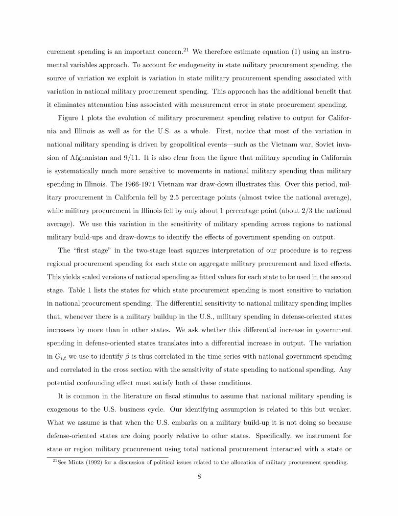
Figure 1 plots the evolution of military procurement spending relative to output for Califor-

nia and Illinois as well as for the U.S. as a whole. First, notice that most of the variation in

national military spending is driven by geopolitical events—such as the Vietnam war, Soviet inva-

sion of Afghanistan and 9/11. It is also clear from the figure that military spending in California

is systematically much more sensitive to movements in national military spending than military

spending in Illinois. The 1966-1971 Vietnam war draw-down illustrates this. Over this period, mil-

itary procurement in California fell by 2.5 percentage points (almost twice the national average),

while military procurement in Illinois fell by only about 1 percentage point (about 2/3 the national

average). We use this variation in the sensitivity of military spending across regions to national

military build-ups and draw-downs to identify the effects of government spending on output.

The “first stage” in the two-stage least squares interpretation of our procedure is to regress

regional procurement spending for each state on aggregate military procurement and fixed effects.

This yields scaled versions of national spending as fitted values for each state to be used in the second

stage. Table 1 lists the states for which state procurement spending is most sensitive to variation

in national procurement spending. The differential sensitivity to national military spending implies

that, whenever there is a military buildup in the U.S., military spending in defense-oriented states

increases by more than in other states. We ask whether this differential increase in government

spending in defense-oriented states translates into a differential increase in output. The variation

in Gi,t we use to identify β is thus correlated in the time series with national government spending

and correlated in the cross section with the sensitivity of state spending to national spending. Any

potential confounding effect must satisfy both of these conditions.

It is common in the literature on fiscal stimulus to assume that national military spending is

exogenous to the U.S. business cycle. Our identifying assumption is related to this but weaker.

What we assume is that when the U.S. embarks on a military build-up it is not doing so because

defense-oriented states are doing poorly relative to other states. Specifically, we instrument for

state or region military procurement using total national procurement interacted with a state or

21See Mintz (1992) for a discussion of political issues related to the allocation of military procurement spending.

8

region dummy.22 We estimate the effects of military spending on employment and inflation using

an analogous approach. For employment, the regression is analogous to equation (1) except that

the left-hand side variable is the two year percentage change in the employment rate—(Lit −

Lit−2)/Lit−2—where Lit is the employment rate (employment divided by population). For the

inflation regression, the left-hand side variable is the two-year inflation rate, (Pit − Pit−2)/Pit−2,

where Pit is the price level.

3.2 Effects of Government Spending Shocks

The results of these regressions are presented in the first row of table 2. For each specification,

the table reports the open economy relative multiplier β. Standard errors are in parentheses and

are clustered by regions or states.23 In the second row of Table 2, we present an analogous set of

results using a broader measure of military spending that combines military procurement spending

with compensation of military employees for each state or region. We present results for output

both deflated by national CPI and our measure of state CPI.

The point estimates of β for the output regression range from 1.4 to 1.9, while the point

estimates of β for the employment regression range from 1.3 to 1.8. The estimates using regional

data are, in general, slightly larger than those based on state data, though the differences are

small and statistically insignificant. The point estimates of the effects of military spending on

consumer prices are statistically insignificantly different from zero, ranging from small positive to

small negative numbers.24

The regressions above control for short-term movements in population associated with govern-

ment spending by looking for relationships among variables in per-capita terms. The last column

of Table 2 characterizes the nature of these population movements. The regression we estimate is

again analogous to equation (1) except that the left-hand side variable is the two year percentage

22Nekarda and Ramey (2010) use a similar approach to purge government purchases for particular industries ofpotentially endogenous responses to industry productivity. They use data at 5 year intervals to estimate the shareof aggregate government spending from different industries, as opposed to the responsiveness of industry output toaggregate spending.

23Our standard errors thus allow for arbitrary correlation over time in the error term for a given state. They alsoallow for heteroskedasticity. As we describe below, we have carried out an extensive Monte Carlo analysis of ourestimator to judge the robustness of our results. The Monte Carlo analysis indicates that while the standard errorfor the state-level regressions is unbiased, the standard errors for the region regressions are slightly downward-biased:the standard 95% confidence interval based on the standard errors reported in table 2 is in fact a 90% confidenceinterval. This adjustment arises from the well-known small-sample bias in clustered standard errors in the presenceof a small number of clusters.

24The difficulty in obtaining a precise estimate of the effect of military spending on inflation no doubt arises inpart from the paucity of the data involved—state and regional inflation data are likely to suffer from a large amountof measurement error. See section 2 for a discussion of the inflation data.

9

change in population—(Popit − Popit−2)/Popit−2—and the right-hand side government spending

variable as well as the instruments are constructed using the level of government spending and

output rather than per-capita versions of these variables. We find government spending shocks to

have small and statistically insignificant effects on population over the time horizon we consider.25

Figure 3 gives a visual representation of our main specification for output. The figure shows

averages of changes in output and predicted military spending (based on our first-stage regression),

grouped by 30 quantiles of the predicted military spending variable. Both variables are demeaned

by year and state fixed effects. The vast majority of points in the figure are located in the NE and

SW quadrants, leading to a positive coefficient in our IV regression. To assess the robustness of

our result, we have experimented with dropping states and regions with especially large estimated

sensitivity of spending to national spending and this slightly raises the estimated multiplier.26

Table 3 presents a number of alternative specifications for the effects of military procurement

on output and employment. We report the output multiplier when per-capita output is constructed

using a measure of the working age population as opposed to the total population.27 We add the

price of oil interacted with state dummies as controls to our baseline regression. We add the real

interest rate interacted with state dummies as controls to our baseline regression. We estimate

the employment regression using the BEA’s employment series (available from 1969) instead of

BLS payroll employment. This series includes estimated values of self-employment and other non-

payroll employment. The table shows that these specifications all yield similar results to our

baseline estimates.

An alternative way to construct instruments for state spending based on national spending is

to scale national spending by the average level of spending in each state relative to state output,

an approach sometimes referred to as constructing “Bartik instruments” (Bartik, 1991; Blanchard

and Katz, 1992). To construct these estimates, we use the average level of spending in the first

five years of our sample, implying that the fraction of military spending is pre-determined relative

to the majority of our sample period. Results for output and employment using this instrument

instead of our baseline instruments are presented in Table 3. For output, this approach yields a

25Blanchard and Katz (1992) show that population dynamics are important in determining the dynamics of unem-ployment over longer horizons.

26MO and CT have substantially higher estimated sensitivity of spending to national spending than other statesand ND has a substantially negative estimated sensitivity (alone among the states). Dropping any combination ofthese states from our baseline regression slightly raises the our multiplier estimate. Dropping all three yields 1.88(0.57).

27State-level measures of population by age-group are available from the Census Bureau starting in 1970. We definethe working age population as the population between the ages of 19 and 64.

10

multiplier of roughly 2.5 with a standard error of 0.9 for the states and 2.8 with a standard error of

0.7 for the regions. For employment, this approach also yields larger multipliers than our baseline

specification.

Table 3 also presents OLS estimates of our baseline specification for output. The OLS estimates

are substantially lower than our instrumental variables estimates. A natural explanation of this

is that states’ elected officials may find it easier to argue for spending at times when their states

are having trouble economically. There is a substantial literature in politics and political economy

supporting this notion (see, e.g. Mintz, 1992). Our instruments also likely correct for measurement

error in the data on state-level prime military contracts that does not arise at the national level.

Such measurement error causes an “attenuation bias” in the OLS coefficient toward zero that is

corrected for in our instrumental variables specifications.28

Table 4 presents the results for equation (1) estimated separately by major SIC/NAICS group-

ings. Statistically significant output responses occur in the construction, manufacturing, retail

and services sectors. The largest output response is in the construction sector, where an increase

in military procurement equal to 1% of state GDP is associated with a 5.4% increase in relative

sectoral output. Given the difficulties of measuring output in the government sector, one might

be concerned that our results on the effects of government spending shocks are driven in part by

increases in output in this sector.29 Table 4 shows that this is not the case; increases in govern-

ment sector output contribute negligibly to the overall effects we estimate. Table 4 also shows that

increases in relative procurement spending are not associated with increases in non-procurement

military output.

We have extensively investigated the small-sample properties of our estimation approach using

Monte Carlo simulations. Our analysis suggests no bias in the level of the region-level multiplier.

However, it suggests that our estimates of the state regressions are likely to be slightly conservative

in the sense of underestimating the fiscal multiplier for states by roughly 10% (implying that

the true state-level multiplier is 1.65 rather than 1.43). Intuitively, this downward bias arises

because instrumental variables does not fully correct for endogeneity in small samples, leading IV

28In section 3.3 below, we describe an alternative source of data on military procurement based on shipments tothe government from defense oriented industries. Notice that, despite the close correspondence between the primemilitary contract data and the shipments data, differences remain in the growth rates for the two series. Viewingthese as independent (but noisy) measures on the magnitude of spending, we can adjust for measurement error byusing one variable as an instrument for the other. We find that this significantly raises the multiplier relative to theOLS estimates.

29The measurement difficulties imply that output in the government sector is typically measured using input costs.

11

to be biased in the direction of OLS.30 The LIML estimator avoids this downward bias in the IV

estimator but yields larger standard errors in both the data (see Table 3) and our Monte Carlo

analysis.31

Our results show that output in defense oriented states and regions is differentially affected by

national military build-ups and draw-downs. A potential concern with interpreting this as evidence

for a large open economy relative multiplier is that defense oriented regions might just happen to

be generally more cyclically sensitive. As it turns out, this is not the case. The standard deviation

of output growth is the same for states and regions with above-median defense orientation as below

median (4.7% for regions and 6.1% for states). Furthermore, suppose we regress state output growth

∆Yit on scaled national output growth si∆Yt, where the scaling factor si is the average level of

military spending in each state relative to state output, as well as state and time fixed effects. If

state with high si are more cyclically sensitive, this regression should yield a positive coefficient on

si∆Yt. In fact, the coefficient is slightly negative in our data. In contrast, when si∆Yt is replaced

with si∆Gt, this regression yields a large positive coefficient.

Ramey (2011) argues that news about military spending leads actual spending by several quar-

ters and that this has important implications for the estimation of fiscal multipliers. When we

add future spending as a regressor in regression (1), the coefficient on this variable is positive and

the sum of the coefficients on the government spending rises somewhat. This suggests that our

baseline specification somewhat underestimates the multiplier by ignoring output effects associated

with anticipated future spending.

30See Stock, Wright, and Yogo (2002) for an overview of this issue. The concern is that the first-stage of the IVprocedure may pick up some of the endogenous variation in the explanatory variable in the presence of a large numberof instruments. In contrast to the canonical examples discussed in Stock, Wright, and Yogo (2002), this actuallybiases us away from finding a statistically significant result in small samples, since the OLS estimates in our caseare close to zero. Our Monte Carlo analysis is roughly consistent with the asymptotic results reported in Stock andYogo (2005). The partial R-squared of the excluded instruments, a statistic frequently used to gauge the “strength”of instruments is 12% for the state regressions and 18% for the region regressions. However, because we use a largenumber of instruments in our baseline case—one for each state or region—the Cragg-Donald (1993) first stage F-statistic suggested by Stock and Yogo (2005) is roughly 5 for our baseline specification of the state-level regressionsand 8 for the region-level regressions. (This statistic is, of course, much higher for the simpler Bartik specificationdiscussed above, since it includes only a single instrument.) Our Monte Carlo analysis indicates that while the largenumber of instruments in the state-level specification leads to a slight downward-bias in the coefficient on governmentspending, the standard error on this coefficient is unbiased because of the high R-squared of our instruments takenas a whole. We thank Marcelo Moreira and Motohiro Yogo for generous advice on this issue.

31See, e.g.,Stock and Yogo (2005) for a discussion of the LIML estimator.

12

3.3 Subcontracting of Prime Military Contracts

An important question with regard to the use of military procurement data is to what extent

the interpretation of these data might be affected by subcontracting of prime military contracts

to surrounding states. To investigate this issue, we use Census Bureau data on shipments to the

government from defense oriented industries. To our knowledge, these data have previously been

used only infrequently in studying the geographical distribution of military spending. They were

not previously available in digital form.32 The Census shipments data are available for the period

1963-1983. Figure 2 illustrates the close relationship between the state-level military procurement

data and the shipments data for several states over this period. To summarize this relationship,

we estimate the following relationship between shipments from a particular state and our measure

of military procurement spending,

MSit = αi + βMPSit + εit, (2)

where MSt is the value of shipments from the Census Bureau data and MPSit is our measure of

military procurement spending. Estimating this regression yields a point estimate of β = 0.96,

indicating that our measure of military procurement moves almost one for one with the value of

shipments from the Census Bureau.

3.4 Government Spending at High Versus Low Unemployment Rates

We next investigate whether the effects of government spending on the economy are larger in periods

when the unemployment rate is already high.33 There are a variety of reasons why this could be the

case. Most often cited is the idea that in an economy with greater slack, expansionary government

spending is less likely to crowd out private consumption or investment.34 In a closed economy, a

second potential source of such differences is the differential response of monetary policy—central

bankers may have less incentive to “lean against the wind” to counteract the effects of government

spending increases if unemployment is already high. This latter effect does not, however, influence

32We digitized these data from microfilm. See section 2 for a discussion of the shipments data.33Gordon and Krenn (2010) estimate substantially larger fiscal multiplier for 1940:Q2-1941:Q2 than for 1940:Q2-

1941:Q4. They attribute the fall in the estimated multiplier in the second half of 1941 to increasingly tight capacityconstraints associated with the large military buildup that was underway at that time.

34This might arise, for example, if unemployment leads to a higher labor supply elasticity (Hall, 2009). Such effectsmight also occur in an economy with downwardly-rigid wages. During a recession, wages lie above their market-clearing level in such a model, making output more sensitive to variation in government spending. These effects arebeyond the scope of the model we present in section 4.

13

the results we report below, since the open economy relative multipliers we consider “difference

out” aggregate monetary and tax policy shocks.

To investigate these issues, we estimate the following regression,

Yit − Yit−2Yit−2

= αi + γt + βhGit −Git−2

Yit−2+ (βl − βh)Il

Git −Git−2Yit−2

+ εit, (3)

where Il is an indicator for a period of low economic slack, and the effects of government spending

in high and low slack periods are given by βh and βl respectively. We define high and low slack

periods in terms of the unemployment rate at the start of the interval over which the government

spending occurs. Specifically, period t is defined as a high slack period if Ut−2 is above its median

value over our sample period.35

Table 5 presents our estimates of equation (3). The point estimates support the view that the

effects of government spending are larger when unemployment is high: depending on the specifi-

cation, the government spending multiplier lies between 2 and 3.5 in the high slackness periods,

substantially above our estimates for the time period as a whole. Given the limited number of

business cycles in our sample, we are not, however, able to estimate these effects with much statis-

tical precision. The difference in the multiplier in the high and low spending periods is moderately

statistically significant (with a P-value of 0.06) only in the case of the state-level output regression.

4 A New Keynesian Model of a Monetary Union

To aid interpretation of the open economy relative multiplier we estimate in section 3 and relate it

to the more conventional closed economy aggregate multiplier, we consider a model economy that

consists of two regions belonging to a monetary and fiscal union. Our model is a relatively standard

New Keynesian model that builds on the framework developed in, e.g., Obstfeld and Rogoff (1995),

Chari, Kehoe, and McGrattan (2002), Benigno and Benigno (2003), Woodford (2003), Benigno and

Woodford (2005) and Gali and Monacelli (2008).

We refer to the regions as “home” and “foreign.” The population of the entire economy is

normalized to one. The population of the home region is denoted by n. Household preferences,

market structure and firm behavior take the same form in both regions. Below, we describe the

economy of the home region.

35The high slack years t according to this measure are: 1966, 1967, 1972-1974, 1976-1988, 1993, 1994, 2004 and2005.

14

4.1 Households

The home region has a continuum of household types indexed by x. A household’s type indicates

the type of labor supplied by that household. Home households of type x seek to maximize their

utility given by

E0

∞∑t=0

βtu(Ct, Lt(x)), (4)

where β denotes the household’s subjective discount factor, Ct denotes household consumption of

a composite consumption good, Lt(x) denotes household supply of differentiated labor input x.

There are an equal (large) number of households of each type.

The composite consumption good in expression (4) is an index given by

Ct =

[φ

1η

HCη−1η

Ht + φ1η

FCη−1η

Ft

] ηη−1

, (5)

where CHt and CFt denote the consumption of composites of home and foreign produced goods,

respectively. The parameter η > 0 denotes the elasticity of substitution between home and foreign

goods and φH and φF are preference parameters that determine the household’s relative preference

for home and foreign goods. It is analytically convenient to normalize φH + φF = 1. If φH > n,

household preferences are biased toward home produced goods.

The subindices, CHt and CFt, are given by

CHt =[∫ 1

0 cht(z)θ−1θ dz

] θθ−1

and CFt =[∫ 1

0 cft(z)θ−1θ dz

] θθ−1 (6)

where cht(z) and cft(z) denote consumption of variety z of home and foreign produced goods,

respectively. There is a continuum of measure one of varieties in each region. The parameter θ > 1

denotes the elasticity of substitution between different varieties.

Goods markets are completely integrated across regions. Home and foreign households thus

face the same prices for each of the differentiated goods produced in the economy. We denote these

prices by pht(z) for home produced goods and pft(z) for foreign produced goods. All prices are

denominated in a common currency called “dollars”.

Households have access to complete financial markets. There are no impediments to trade in

financial securities across regions. Home households of type x face a flow budget constraint given

by

PtCt + Et[Mt,t+1Bt+1(x)] ≤ Bt(x) +Wt(x)Lt(x) +

∫ 1

0Ξht(z)dz − Tt, (7)

where Pt is a price index that gives the minimum price of a unit of the consumption good Ct,

Bt+1(x) is a random variable that denotes the state contingent payoff of the portfolio of financial

15

securities held by households of type x at the beginning of period t + 1, Mt,t+1 is the stochastic

discount factor that prices these payoffs in period t, Wt(x) denotes the wage rate received by home

households of type x in period t, Ξht(z) is the profit of home firm z in period t and Tt denotes lump

sum taxes.36 To rule out Ponzi schemes, household debt cannot exceed the present value of future

income in any state of the world.

Households face a decision in each period about how much to spend on consumption, how many

hours of labor to supply, how much to consume of each differentiated good produced in the economy

and what portfolio of assets to purchase. Optimal choice regarding the trade-off between current

consumption and consumption in different states in the future yields the following consumption

Euler equation:uc(Ct+j , Lt+j(x))

uc(Ct, Lt(x))=Mt,t+j

βjPt+jPt

(8)

as well as a standard transversality condition. Subscripts on the function u denote partial deriva-

tives. Equation (8) holds state-by-state for all j > 0. Optimal choice regarding the intratemporal

trade-off between current consumption and current labor supply yields a labor supply equation:

u`(Ct, Lt(x))

uc(Ct, Lt(x))=Wt(x)

Pt. (9)

Households optimally choose to minimize the cost of attaining the level of consumption Ct. This

implies the following demand curves for home and foreign goods and for each of the differentiated

products produced in the economy:

CH,t = φHCt

(PHtPt

)−ηand CF,t = φFCt

(PFtPt

)−η, (10)

cht(z) = CHt

(pt(z)PHt

)−θand cft(z) = CFt

(pt(z)PFt

)−θ, (11)

where

PHt =[∫ 1

0 pt(z)1−θdz

] 11−θ

and P ∗Ft =[∫ 1

0 p∗t (z)

1−θdz] 1

1−θ, (12)

and

Pt =[φHP

1−ηHt + φFP

1−ηF t

] 11−η

. (13)

As we noted above, the problem of the foreign household is analogous. We therefore refrain

from describing it in detail here. It is, however, useful to note that combining the home and foreign

36The stochastic discount factor Mt,t+1 is a random variable over states in period t + 1. For each such state itequals the price of the Arrow-Debreu asset that pays off in that state divided by the conditional probability of thatstate. See Cochrane (2005) for a detailed discussion.

16

consumption Euler equations to eliminate the common stochastic discount factor yields

uc(C∗t , L

∗t (x))

uc(Ct, Lt(x))= Qt, (14)

where Qt = P ∗t /Pt is the real exchange rate. This is the “Backus-Smith” condition that describes

optimal risk-sharing between home and foreign households (Backus and Smith, 1993). For simplic-

ity, we assume that all households—in both regions—initially have an equal amount of financial

wealth.

4.2 The Government

The economy has a federal government that conducts fiscal and monetary policy. Total government

spending in the home and foreign region follow an exogenous AR(1) process. Let GHt denote

government spending per capita in the home region. Total government spending in the home

region is then nGHt. For simplicity, we assume that government demand for the differentiated

products produced in each region takes the same CES form as private demand. In other words, we

assume that

ght(z) = GHt

(pht(z)PHt

)−θand gft(z) = GFt

(pft(z)PFt

)−θ. (15)

The government levies lump-sum taxes to pay for its purchases of goods. Our assumption of

perfect financial markets implies that any risk associated with variation in taxes and transfers across

the two regions is undone through risk-sharing. Ricardian equivalence holds in our model. Windfall

government transfers from one region to the other and lump-sum taxes to finance government

spending in one region, therefore, have no effect on equilibrium allocations in our model. Also, we

need not specify the time-path or regional incidence of taxes.

The federal government operates a common monetary policy for the two regions. This policy

consists of the following augmented Taylor-rule for the economy-wide nominal interest rate:

rnt = ρrrnt−1 + (1 − ρi)(φππ

agt + φyy

agt + φg g

agt ), (16)

where hatted variables denote percentage deviations from steady state. The nominal interest rate

is denoted rnt . It responds to variation in the weighted average of consumer price inflation in the

two regions πagt = nπt + (1 − n)π∗t , where πt is consumer price inflation in the home region and

π∗t is consumer price inflation in the foreign region. It also responds to variation in the weighted

average of output in the two regions yagt = nyt + (1 − n)y∗t . Finally, it may respond directly to the

weighted average of the government spending shock in the two regions gagt = ngt + (1 − n)g∗t .

17

4.3 Firms

There is a continuum of firms indexed by z in the home region. Firm z specializes in the production

of differentiated good z, the output of which we denote yt(z). In our baseline model, labor is the only

variable factor of production used by firms.37 Each firm is endowed with a fixed, non-depreciating

stock of capital. Labor is immobile across regions.38 We follow Woodford (2003) in assuming that

each firm belongs to an industry x and that there are many firms in each industry. The goods in

industry x are produced using labor of type x and all firms in industry x change prices at the same

time.

The production function of firm z is

yt(z) = f(Lt(z)). (17)

The function f is increasing and concave. It is concave because there are diminishing marginal

returns to labor given the fixed amount of other inputs employed at the firm.

Firm z acts to maximize its value,

Et

∞∑j=0

Mt,t+j [pt+j(z)yt+j(z) −Wt+j(x)Lt+j(z)]. (18)

Firm z must satisfy demand for its product. The demand for firm z’s product comes from three

sources: home consumers, foreign consumers and the government. It is given by

yt(z) = (nCHt + (1 − n)C∗Ht + nGHt)

(pht(z)

PHt

)−θ. (19)

Firm z is therefore subject to the following constraint:

(nCHt + (1 − n)C∗Ht + nGHt)

(pht(z)

PHt

)−θ≤ f(Lt(z)). (20)

Firm z takes its industry wage Wt(x) as given. Optimal choice of labor demand by the firm is

given by

Wt(x) = f`(Lt(z))St(z), (21)

where St(z) denotes the firm’s nominal marginal cost (the Lagrange multiplier on equation (20) in

the firm’s constrained optimization problem).

37Appendix B develops an extension of our baseline model with capital.38Our results in section 3, suggest that this is a reasonable assumption over the horizons we focus on. An extension

of our model that allows for an equal amount of labor and capital mobility yields virtually identical results for outputas long as all variables (output, employment, government spending, etc.) are defined in per-capita terms. Blanchardand Katz (1992) emphasize that labor mobility plays an important role in the adjustment to regional shocks overlonger horizons.

18

Firm z can reoptimize its price with probability 1 − α as in Calvo (1983). With probability α

it must keep its price unchanged. Optimal price setting by firm z in periods when it can change

its price implies

Et

∞∑j=0

αjMt,t+j(nCHt+j + (1 − n)CFt+j + nGHt+j)PθHt+j(1 − θ)[pt(z) −

θ

θ − 1St+j(z)] = 0. (22)

4.4 Calibration

We analyze the behavior of the economy for several specific sets of assumptions about the utility

function, production function, monetary policy and parameters of the model. We consider the

following two forms for the utility function:

u(Ct, Lt(x)) =C1−σ−1

t

1 − σ−1− χ

Lt(x)1+ν−1

1 + ν−1, (23)

u(Ct, Lt(x)) =(Ct − χLt(x)1−ν

−1/(1 − ν−1))1−σ

−1

1 − σ−1. (24)

In the first utility specification, consumption and labor enter separably. They are therefore neither

complements nor substitutes. The second utility function is adopted from Greenwood, Hercowitz,

and Huffman (1988). We refer to this utility function as GHH preferences. Consumption and

labor are complements for households with GHH preferences. Recently, Monacelli and Perotti

(2008), Bilbiie (2009), and Hall (2009) have emphasized the implications of consumption-labor

complementarities for the government spending multiplier.

For both specifications for utility, we must specify values for σ and ν (χ is irrelevant when utility

is separable and determined by other parameters in the GHH case). In both cases, ν is the Frisch

elasticity of labor supply. There is little agreement on the appropriate value for this parameter in

the literature. We set ν = 1. This value is somewhat higher than values estimated for employed

workers. The higher value is meant to capture variation in labor on the extensive margin—such as

variation in unemployment and retirement (Hall, 2009). We set σ = 1. For the separable utility

specification, σ denotes the intertemporal elasticity of substitution (IES). There is little agreement

within the macroeconomics literature on the appropriate values for the IES. Hall (1988) estimates

the IES to be close to zero, while Bansal and Yaron (2004), Gruber (2006) and Nakamura, et al.

(2011) argue for values above 1. For the model with separable preferences, σ = 1 yields balanced

growth.

We set the subjective discount factor equal to β = 0.99, the elasticity of substitution across

varieties equal to θ = 7 and the elasticity of substitution between home and foreign goods to η = 2.

19

We assume the production function f(Lt(z)) = Lt(z)a and we set a = 2/3. We set α = 0.75. This

implies that firms reoptimize there prices on average once a year.

We set the size of the home region to n = 0.1. This roughly corresponds to the size of the

average region in our regional regressions (where we divide the U.S. into 10 regions). We use

data from the U.S. Commodity Flow Survey (CFS) and the U.S. National Income and Product

Accounts (NIPA) to set the home-bias parameter φH . The CFS reports data on shipments of goods

within and between states in the U.S. It covers shipments between establishments in the mining,

manufacturing, wholesale and retail sectors. For the average state in 2002, 38% of shipments were

within state and 50% of shipments were within region. However, roughly 40% of all shipments in

the CFS are from wholesalers to retailers and the results of Hillberry and Hummels (2003) suggest

that a large majority of these are likely to be within region. Since the relevant shipments for our

model are those from manufacturers to wholesalers, we assume that 83% of these are from another

region (50 of the remaining 60 percent of shipments).

NIPA data indicate that goods represent roughly 30% of U.S. GDP. If all inter-region trade were

in goods—i.e., all services were local—imports from other regions would amount to 25% of total

consumption (30*0.83 = 25). However, for the U.S. as a whole, services represent roughly 20% of

international trade. Assuming that services represent the same fraction of cross-border trade for

regions, total inter-region trade is 31% of region GDP (25/0.8 = 31). We therefore set φH = 0.69.

This makes our regions slightly more open than Spain and slightly less open than Portugal. We

set φH∗ so that overall demand for home products as a fraction of overall demand for all products

is equal to the size of the home population relative to the total population of the economy. This

implies that φH∗ = (n/(1 − n))φF .

We consider three specifications of monetary policy. First, we consider a specification that is

meant to mimic the policy of the U.S. Federal Reserve during the Volcker-Greenspan period. Many

recent papers have estimated monetary rules similar to the one we adopt for the Volcker-Greenspan

period (see, e.g., Taylor, 1993 and 1999; Clarida, Gali and Gertler, 2000). Guided by this literature

we refer to ρ = 0.8, φπ = 1.5, φy = 0.5 and φg = 0 as the Volcker-Greenspan policy. Notice that

the Volcker-Greenspan policy is one in which the monetary authority “leans against the wind” in

the sense that it raises the real interest rate in response to inflationary shocks.

The second monetary policy we consider is one that responds directly to the fiscal policy shock

in such a way as to neutralize the effect that such shocks have on the real interest rate. In other

words, this policy maintains a constant real interest rate when fiscal policy shocks occur. We

20

refer to this policy as the constant real interest rate policy. This policy does not lean against the

wind in response to government spending shocks. To guarantee price level determinacy, we must

rule out self-fulfilling variation in inflation that is not driven by fundamental shocks (i.e., sunspot

equilibria). We do this by setting φπ = 1.5. This implies that the real interest rate will react to

any variation in inflation that is not caused by government spending shocks. Along the equilibrium

path, no such variation occurs in our model.

The third policy specification we consider is one that maintains a constant nominal interest rate

when fiscal policy shocks occur. We refer to this policy as the constant nominal interest rate policy.

This policy is meant to mimic monetary policy at the zero lower bound. Again, to guarantee price

level determinacy, the constant nominal interest rate policy has φπ = 1.5.

We set the steady state value of government purchases as a fraction of output to 0.2. We set

the AR(1) coefficient on the government spending shock such that the half-life of the government

spending shock is 2 years (i.e. an AR(1) coefficient of 0.51/8 ≈ 0.917) to roughly match the

persistence of aggregate military procurement spending in the data. We log-linearize the equilibrium

conditions of the model and use the methods of Sims (2001) to find the unique bounded equilibrium.

5 Government Spending in a New Keynesian Model

In this section, we analyze the effects of fiscal policy shocks in the model presented in section 4.

5.1 The Closed Economy Aggregate Multiplier

Consider first the standard closed economy aggregate multiplier, calculated as the response of

total output (combining home and foreign production) to total government spending. To estimate

the closed economy aggregate multiplier, we simulate data from the model described in section 4

and estimate a closed economy version of equation (1). Specifically, we use aggregate output and

aggregate government spending to construct the dependent and independent variables and we no

longer include fixed effects in the regression. To compute the same objects in the data and model,

we time-aggregate quarterly data from the model to an annual frequency to estimate equation (1).

The first panel of table 6 reports results for the model in section 4 for the standard case of

household preferences that are additively separable between consumption and labor. The first

column reports results on the closed economy aggregate multiplier. We present results for three

different monetary policies that differ in the degree to which movements in the interest rate are used

21

to “lean against the wind” in response to the government spending shock—a Volcker-Greenspan

monetary policy in which real interest rates are assumed to rise in response to increasing output

or inflation, a fixed real interest rate rule, and a fixed nominal interest rate rule meant to mimic

monetary policy at the zero lower bound.

The model with a Volcker-Greenspan monetary policy yields a closed economy aggregate output

multiplier of only 0.22. With the constant real interest rate monetary policy, the closed economy

multiplier is one. The multiplier is higher because monetary policy leans less against the wind—the

real interest rate remains constant rather than rising when spending increases. Woodford (2010)

shows that for a constant real interest rate monetary policy, the closed economy multiplier is one for

a broad set of parameter values in models without capital. Intuitively, consumption doesn’t change

since the real interest rate is constant. Output must therefore rise one-for-one with government

spending.

Finally, we report results for constant nominal interest rate monetary policy. This is a close

cousin of monetary policy at the zero-lower bound, a scenario analyzed in detail by Eggertsson

(2010), Christiano, Eichenbaum, and Rebelo (2010), and Mertens and Ravn (2010). This policy

has the potential to generate extremely large multipliers since expansionary fiscal policy, by raising

inflationary expectations, drives down real interest rates, leading to further increases in consumption

and output. In our framework, the closed economy aggregate multiplier is 1.70 if the nominal

interest rate is fixed and the government spending shock has a half-life of one year (i.e., ρg = 0.85).

This result is, however, sensitive to the persistence of the government spending shock. For our

baseline parameters, where government spending is slightly more persistent (ρg = 0.917), the

closed economy aggregate multiplier falls to -0.39.39

Needless to say, the rise in aggregate GDP that arises if the government buys more output is

highly sensitive to the stance of monetary policy. This sensitivity carries over to other variables.

Much recent work on the effects of fiscal policy has focused on consumption, real wages and markups

(Ramey, 2010; Perotti, 2007). Our closed economy New Keynesian model with Volcker-Greenspan

monetary policy generates a fall in all three of these variables in response to positive government

spending shocks, while the same exercise with the constant real interest rate monetary policy yields

39The sensitivity of the fixed nominal interest rate multiplier to the persistence of government spending is closelyrelated to issues discussed in Mertens and Ravn (2010). Intuitively, the government spending shock has both de-flationary effects (for a given level of output, it increases labor supply and thus reduces marginal costs by reducingconsumption) and inflationary effects (it increases demand at a given interest rate since households would like tosmooth consumption). Which effect is bigger depends on the persistence of the government spending shock. Withhighly persistent government spending shocks, the deflationary effect dominates (demand does not increase by muchbecause the shock has a large effect on permanent income).

22

an increase in real wages and markups, and leaves consumption unchanged.

This sensitivity of the multiplier to the stance of monetary policy may help to explain some

of the wide range of estimates of the multiplier in the empirical literature. Most economists agree

that the extent to which the Federal Reserve has “leaned against the wind” has varied substantially

over the last century. Many economists believe, for example, that monetary policy was far more

expansionary during the 2007-2009 financial crisis than in earlier financial crises such as the Great

Depression.

The sensitivity of the closed economy aggregate multiplier to the stance of monetary policy

makes it difficult to distinguish between alternative models of the economy. The last row in Panel

A Table 6 presents results for a version of our model with flexible prices. The closed economy

aggregate multiplier in this case is 0.39, which lies well within the range of multipliers for the New

Keynesian model for alternative monetary policies. While the Neoclassical and New Keynesian

models may yield similar government spending multipliers under responsive monetary policies such

as the Volcker-Greenspan policy, their implications can differ greatly when nominal interest rates

are fixed—such as when interest rates hit the zero lower bound. The Neoclassical model continues to

yield a small multiplier in this case, whereas the New Keynesian multiplier is potentially very large.

Thus, while the predictions of New Keynesian and Neoclassical models for the effects of government

spending may be difficult to tell apart in normal times, the distinction may be crucially important

in times of crisis.

5.2 The Open Economy Relative Multiplier

Contrast the wide range of different closed economy aggregate multipliers produced by our model

for different monetary policies with the complete stability of the open economy relative multiplier

reported in the second data column of Table 6. This open economy relative multiplier is calculated

by estimating equation (1) using the regional data from the model. For all three specifications of

monetary policy we consider, this open economy relative output multiplier is 0.85. In other words,

the open economy relative multiplier in our model is completely insensitive to the specification of

monetary policy.40

The intuition for this result rests on the fact that in estimating the open economy relative

multiplier we “difference out” aggregate shocks affecting the economy by including time fixed

40The open economy relative multiplier is, of course, not completely insensitive to other parameters of the model,such as the persistence of the government spending shock, as can be seen from the fourth row of the table.

23

effects in the regression. Since the different regions share the same monetary policy, this procedure

differences out the aggregate effects of monetary policy. What we measure is the differential effect of

government spending on output across regions. Since the two regions belong to a monetary union,

monetary policy in one region cannot differentially respond to regions spending shocks. This implies

that the open economy relative multiplier is akin to a closed economy aggregate multiplier for a

relatively accommodating aggregate monetary policy. Readers familiar with the Mundell-Fleming

model will recall that the fiscal multiplier in that model is larger under a fixed exchange rate than

a flexible exchange rate for the same reason.

The open economy relative multiplier we estimate turns out the be equal to the aggregate

multiplier in a small open economy with a fixed exchange rate. We have verified this by letting the

size of the home country go to zero and calculating the aggregate multiplier for that country in the

limit. Intuitively, if the home country is sufficiently small, it has a negligible effect on the currency

union as a whole. As a consequence, the ”relative” effect of government spending will be the same

as the aggregate effect on the home region—i.e., the time dummies will be zero in equation (1).

Since the relative nominal interest rate is constant in response to a government spending shock

in one region—i.e., the monetary authority cannot respond to the shock by making monetary policy

tighter in that region alone—it is tempting to assume that this situation is analogous to the response

of a close economy to a government spending shock at the zero lower bound. In fact, an increase in

government spending in the home region leads to a rise in expected inflation, lowering real interest

rates—just as in the closed economy case at the zero lower bound.

This logic turns out to ignore a crucial aspect of our setting. The crucial difference versus the

closed economy zero lower bound setting is that in our setting, the long-term real interest rate does

not fall in response to the fiscal shock, even though the short-term real interest rate does. The

fiscal shock leads to an immediate rise in prices and expectations of further rises in prices in the

short term. This lowers the short term real interest rate. However, since purchasing power parity

must hold in the long run, any short term increase in prices in one region relative to the other

region must be undone by a fall in prices in that region later on. This means that the long term

real interest rate does not fall in our setting. In fact, the initial jump up in prices implies that

going forward prices are anticipated to fall more in the long run than they are anticipated to rise

further in the short run. This implies that the relative long-term real interest rate actually rises

slightly in the home region in response to an increase in government spending.41

41Corsetti et al. (2011) explore this effect for the case of a small open economy with a fixed exchange rate.

24

Since the relevant interest rate—the long-term real interest rate—actually rises slightly in re-

sponse to an increase in government spending irrespective of the persistence of the shock and other

parameters, the fixed relative nominal interest rate policy in a monetary union is fundamentally

different from a fixed nominal interest rate policy in a closed economy setting with a Taylor rule

monetary policy. The response of long-term real interest rates in our setting is closest to the fixed

real interest rate case in the closed economy setting, where the output multiplier equals 1.0. Policy

in our case is slightly more contractionary (since long-term real interest rates actually rise a slight

bit). Table 6 shows that the open economy relative multiplier is, in fact, 0.85 for our baseline

parameter values—far below the fixed nominal rate multipliers emphasized by Eggertsson (2010)

and Christiano, Eichenbaum, and Rebelo (2010) and just slightly lower than the closed economy

aggregate multiplier for a fixed real rate monetary policy.

To more clearly see the intuition for this result, Figure 4 presents the impulse response of

the price level and the real interest rate in the home region relative to the foreign region after a

government spending shock in our model. The home price level rises for several periods, but then

falls back to its original level of purchasing power parity. This movement in prices implies that the

real interest rate in the home region initially falls, but then rises above its steady state level for a

prolonged period. Figure 5 shows what happens to consumption in the home region relative to the

foreign region after a government spending shock in our model. Despite the short-run fall in the

real interest rate, consumption falls. This is because households anticipate high real rates in the

future—equivalently, they face a high current long-term real interest rate—and therefore cut their

consumption.

5.3 GHH Preferences

The results discussed above show that both the Neoclassical model and the benchmark New Key-

nesian model yield open economy relative multiplier that are quite a bit smaller than our empirical

estimate. To bring our models better in line with the empirical evidence, we allow for comple-

mentarities between consumption and work. In particular, panel B of Table 6 reports results for

a model with consumption-labor complementarities in the form of GHH preferences. Recent work

by Monacelli and Perotti (2008), Bilbiie (2009), and Hall (2009) has shown that such complemen-

tarities have the potential to raise the government spending multiplier. Aguiar and Hurst (2005)

25

present empirical evidence for such complementarities.42

With GHH preferences, the closed economy aggregate multipliers are even more sensitive to

monetary policy: ranging from -1 to almost 9. The table makes clear, furthermore, that GHH

preferences can either raise or lower the closed economy aggregate multiplier in comparison to the

model with separable preferences. If monetary policy is relatively unresponsive to increases in

output as in the constant real rate case, we find that incorporating GHH preferences raises the

closed economy aggregate multiplier. However, if monetary policy is highly responsive to output

as in the Volcker-Greenspan policy, GHH preferences lead to lower multipliers. The Neoclassical

(flexible price) model yields a multiplier of zero since the wealth effect on labor supply is absent.43

This is well within the range of multipliers implied by the New Keynesian model for alternative

monetary policies as in the separable utility case.

The second data column of Panel B of Table 6 reports results for the open economy relative

multiplier. It is 1.48 for all three specifications of our benchmark model (ρg = 0.917) and 2.09

for the case of more transitory government spending shocks (ρg = 0.5). Incorporating GHH pref-

erences unambiguously raises our open economy relative multiplier. This arises because, as we

describe above, real interest rates rise only slightly to offset higher output in a particular region

in the monetary union. Since the monetary policy is effectively quite unresponsive to local shocks,

the complementarity between consumption and work embodied in GHH preferences raises the mul-

tiplier. Intuitively, since households are working more and consumption is complementary to labor,

their demand for consumption is larger than in the model with separable preferences. But to be

able to consume more, still more production must take place. Firms with rigid prices meet this

demand and bid up real wages in the process. This shifts the trade-off between more work and less

consumption further towards more work and thus increases the output multiplier—so long as real

interest rates do not rise too much in response to the increase in output.

Figure 6 plots relative output and consumption in our open economy model with GHH pref-

erences after a positive shock to home government spending. Both output and consumption rise

on impact by a little more than twice the amount of the shock. They then both fall more rapidly

than the shock. The fact that the initial rise in consumption is as large as the rise in output

implies that the home region responds to the shock by running a trade deficit in the short run.

42Schmitt-Grohe and Uribe (2009) estimate a rich business cycle model with Jaimovich and Rebelo (2009)preferences—which nests GHH and King and Rebelo (1988) preferences as special cases. Their estimates showthat the data strongly prefers parameters that give GHH preferences.

43With sticky prices government spending shocks affect the markup of prices over marginal costs and thereforeaffect output by shifting labor demand.

26

Consumption eventually falls below its steady state level for a period of time. During this time

the home region is running a trade surplus. Intuitively, the complementarity between consumption

and labor implies that home households want to shift their consumption towards periods of high

work effort associated with positive government spending shocks.

Summing up our results thus far, our estimates of equation (1) based on the military procure-

ment data yield an open economy relative multiplier of roughly 1.5. This lies far above the open

economy relative multipliers for the Neoclassical model—which are roughly 0.5 for both separable

preferences and GHH preferences. Our empirical estimate of 1.5 is also substantially higher than

the open economy relative multiplier of 0.85 implied by the New Keynesian model with separable

preferences. The New Keynesian model with GHH preferences, however, is able to match the open

economy relative multiplier we estimate in the data.44 The fact that the open economy relative

multiplier is not sensitive to aggregate monetary (or tax) policy implies that it is a powerful statis-

tic for distinguishing between different models of the economy. In contrast, the closed economy

aggregate multiplier is highly sensitive to aggregate policy and thus less easily used to distinguish

between models.

5.4 Model with Capital

Appendix B develops an extension of the model presented in section 4 that includes investment,

capital accumulation and variable capital utilization. The specification for these features that we

adopt mirrors closely that of Christiano, Eichenbaum, and Evans (2005). Open economy relative

multipliers for several calibrations of this model with GHH preferences are presented in Table 7.

The main conclusion is that introducing capital into the model lowers the multiplier somewhat.

Intuitively, in this model, government spending “crowds out” investment. One way to match the

multiplier in the data for this model is to raise the elasticity of labor substantially (to 25). Table 7

also presents open economy relative multiplier for employment and prices. The Neoclassical model

implies much larger movements in relative prices than does the New Keynesian model. We find

little evidence for large movements in relative prices in the data. This is thus another empirical

prediction that favors the New Keynesian model over the Neoclassical model.

44Models with hand-to-mouth consumers of the type studied by Gali, Lopez-Salido, and Valles (2007) may alsohave the potential to generate large open economy relative multipliers.

27

6 Conclusion

We study the effects of government spending on output in a monetary union. Our empirical

analysis makes use of historical data on military procurement spending across U.S. regions. We

measure the consequences of a differential increase in government spending in a particular region on

output, employment, and prices in that region relative to other regions in the union. Since regional

procurement spending potentially responds to underlying economic conditions in the region, we

focus only on the effects of relative changes in government spending that arise from aggregate

military build-ups or draw-downs. We use time fixed effects to control for aggregate shocks that

affect all regions. Our estimates imply an open economy relative output multiplier of approximately

1.5.

We develop a framework for interpreting this open economy relative multiplier and relating it

to estimates of closed economy aggregate multipliers. The closed economy aggregate multiplier

is highly sensitive to how strongly aggregate monetary and tax policy “leans against the wind.”

In contrast, the open economy relative multiplier “differences out” these effects because different

regions in the union share a common monetary and tax policy. Since the monetary authority

cannot raise interest rates differentially in one region relative to other regions in response to a

regions spending shock, our open economy relative multiplier is akin to an aggregate multiplier for

a more accommodative monetary policy than the monetary policy seen in the United States. This

implies that our open economy relative multiplier of 1.5 is not inconsistent with lower aggregate

multipliers found in the literature.

Our estimate provides evidence in favor of models in which demand shocks can have large effects

on output. We show that a New Keynesian model with complementarities between consumption

and work in the form of GHH preferences yields an open economy relative multiplier that matches

our empirical estimate. Baseline New Keynesian and Neoclassical models, however, yield lower

open economy relative multipliers.

28

A Constant Real Rate Monetary Policy

The paper considers specifications of monetary policy that hold the real or nominal interest rate

constant in response to a government spending shock. Here, we illustrate the method used to solve

for these monetary policy specifications. We do this for the case of separable preference and a

monetary policy that holds the real interest rate constant. The GHH preference case and the case

of holding the nominal interest rate constant are similar.

Consider the closed economy limit of our model. A log-linear approximation of the key equilib-

rium conditions of this model are

ct = Etct+1 − σ(rnt − Etπt+1), (25)

πt = βEtπt+1 + κζσ−1ct + κζψν yt, (26)

yt =

(C

Y

)ct + gt, (27)

where ζ = 1/(1 + ψνθ) and ψν = (1 − ν−1)/a− 1.

Using equation (27) to eliminate ct from equations (25) and (26) yields

yt = Etyt+1 −(C

Y

)σ(rnt − Etπt+1) + (gt − Etgt+1), (28)

πt = βEtπt+1 + κζyyt − κζg gt, (29)

where ζy = ζ(ψν + (C/Y )−1σ−1) and ζg = ζ(C/Y )−1σ−1.

An equilibrium with a fixed real interest rate must satisfy

yt = Etyt+1 + (gt − Etgt+1), (30)

πt = βEtπt+1 + κζyyt − κζg gt. (31)

We conjecture a solution of the form y∗t = ay gt, π∗t = aπ gt. Using the method of undetermined

coefficients, it is easy to verify that such an equilibrium exists with

ay = 1, aπ = κζy−ζg1−βρg ,

where ρg is the autoregressive coefficient of the AR(1) process for gt.

This equilibrium can be implemented with the following policy rule

rnt = Etπt+1 + φπ(πt − π∗t )

= aπρg gt + φππt − aπφπ gt

= φππt − aπ(φπ − ρg)gt. (32)

29

B Model with Capital

This appendix presents the an extension of the model presented in section 4 that incorporates

investment, capital accumulation and variable capital utilization. We adopt a specification for

these features that mirrors closely the specification in Christiano, Eichenbaum, and Evans (2005).

B.1 Households

Household preferences in the home region are given by equations (4)-(6) as before. Household

decisions regarding consumption, saving and labor supply are thus the same as before. However,

in addition to these choices, households own the capital stock, they choose how much to invest and

they choose the rate of utilization of the capital stock. Let Kt denote the physical stock capital of

capital available for use in period t and It the amount of investment chosen by the household in

period t. For simplicity, assume that It is a composite investment good given by an index of all the

products produced in the economy analogous to equations (5)-(6) for consumption. The capital

stock evolves according to

Kt+1 = (1 − δ)Kt + Φ(It, It−1), (33)

where δ denotes the physical depreciation of capital and Φ summarizes the technology for trans-

forming current and past investment into capital. Households choose the utilization rate ut of the

capital cost. The amount of capital services provided by the capital cost in period t is then given

by Kt = utKt.

The budget constrain of households’ in the home region is given by

PtCt + PtIt + PtA(ut)Kt + Et[Mt,t+1Bt+1(x)]

≤ Bt(x) +Wt(x)Lt(x) +Rkt utKt +

∫ 1

0Ξht(z)dz − Tt. (34)

The differences relative to the model presented in section 4 are: First, households spend PtIt

on investment. Second, they incur a cost PtA(ut)Kt associated with utilizing the capital stock.

Here A(ut) denotes a convex cost function. Third, they receive rental income equal to Rkt utKt for

supplying utKt in capital services. Here Rkt denotes the rental rate for a unit of capital services.

In addition to equations (8)-(11), (14) and a standard transversality condition, household op-

timization yields the following relevant optimality conditions. Optimal capital utilization sets the

marginal cost of additional utilization equal to the rental rate on capital,

A′(ut) =RktPt. (35)

30

Optimal investment and capital accumulation imply

DtΦ1(It, It−1) + βEt[Dt+1Φ2(It+1, It)] = uc(Ct, Lt(x)), (36)

Dt = β(1 − δ)EtDt+1 + βEt[(A′(ut+1)ut+1 −A(ut+1))uc(Ct+1, Lt+1(x))], (37)

where Dt is the Lagrange multiplier on equation (33) and Φj(·, ·) denotes the derivative of Φ with

respect to its jth argument.

B.2 Firms

The production function for firm z is

yt(z) = f(Lt(z),Kt(z)). (38)

The demand for firm z’s product is given by

yt(z) = (nCHt + (1 − n)C∗Ht + nIH,t + (1 − n)I∗H,t + nGHt)

(pht(z)

PHt

)−θ. (39)

Firm optimization then yields

Wt(x) = f`(Lt(z),Kt(z))St(z), (40)

Rkt = fk(Lt(z),Kt(z))St(z), (41)

and a firm price setting equation given by equation (22).

B.3 Calibration

We set the rate of depreciation of capital to δ = 0.025, which implies an annual depreciation rate

of 10 percent. The investment adjustment cost function is given by

Φ(It, It−1) =

[1 − φ

(ItIt−1

)]It, (42)

where φ(1) = φ′(1) = 0 and κI = φ′′(1) > 0. We set κI = 2.5. This is the value estimated by

Christiano et al. (2005). We require that capital utilization ut = 1 in steady state, assume that

the cost of utilization function A1 = 0 and set σa = A′′(1)/A′(1) = 0.01. Again, this is the value

estimated by Christiano et al. (2005). We assume that the production function is Cobb-Douglas

with a capital share of 1/3.

31

References

Acconcia, A., G. Corsetti, and S. Simonelli (2011): “Mafia and Public Spending: Evidenceon the Fiscal Multiplier from a Quasi-Experiment,” CEPR Discussion Paper No. 8305.

Aguiar, M., and E. Hurst (2005): “Consumption versus Expenditure,” Journal of PoliticalEconomy, 113(5), 919–948.

Alesina, A., and S. Ardagna (2009): “Large Changes in Fiscal Policy: Taxes versus Spending,”in Tax Policy and the Economy, Volume 24, ed. by J. R. Brown, pp. 35–68, Chicago IL. Universityof Chicago Press.

Auerbach, A. J., and Y. Gorodnichenko (2010): “Measuring the Output Responses to FiscalPolicy,” NBER Working Paper No. 16311.

Backus, D. K., and G. W. Smith (1993): “Consumption and Real Exchange Rates in DynamicEconomies with Non-Traded Goods,” Journal of International Economics, 35(3–4), 297–316.

Bansal, R., and A. Yaron (2004): “Risks for the Long Run: A Potential Resolution of AssetPricing Puzzles,” Journal of Finance, 59(4), 1481–1509.

Barro, R. J., and C. J. Redlick (2011): “Macroeconomic Effects from Government Purchasesand Taxes,” Quarterly Journal of Economics, 126, Forthcoming.

Bartik, T. J. (1991): Who Benefits from State and Local Economic Development Policies? W.E.Upjohn Institute for Employment Research, Kalamazoo, MI.

Baxter, M., and R. G. King (1993): “Fiscal Policy in General Equilibrium,” American EconomicReview, 83(3), 315–334.

Benigno, G., and P. Benigno (2003): “Price Stability in Open Economies,” Review of EconomicStudies, 70(4), 743–764.

Benigno, P., and M. Woodford (2005): “Inflation Stabilization and Welfare: The Case of aDistorted Steady State,” Journal of the European Economic Association, 3, 1185–1236.

Bilbiie, F. O. (2009): “Non-Separable Preferences, Frisch Labor Supply and the ConsumptionMultiplier of Government Spending: One Solution to a Fiscal Policy Puzzle,” Working Paper,Paris School of Economics.

Blanchard, O., and R. Perotti (2002): “An Empirical Characterization of the Dynamic Effectsof Changes in Government Spending,” Quarterly Journal of Economics, 117(4), 1329–1368.

Blanchard, O. J., and L. Katz (1992): “Regional Evolutions,” Brookings Papers on EconomicActivity, 1992(1), 1–75.

Braddon, D. (1995): “The Regional Impact of Defense Expenditure,” in Handbook of DefenseEconomics, ed. by K. Hartley, and T. Sandler, pp. 491–521, Amsterdam. Elsevier Science.

Burnside, C., M. Eichenbaum, and J. Fisher (2004): “Fiscal Shocks and their Consequences,”Journal of Economic Theory, 115, 89–117.

Calvo, G. A. (1983): “Staggered Prices in a Utility-Maximizing Framework,” Journal of MonetaryEconomics, 12, 383–398.

Canova, F., and E. Pappa (2007): “Price Differentials in Monetary Unions: The Role of FiscalShocks,” The Economic Journal, 117(520), 713–737.

32

Chari, V., P. J. Kehoe, and E. R. McGrattan (2002): “Can Sticky Price Models GenerateVolatile and Persistent Real Exchange Rates,” Review of Economic Studies, 69, 533–563.

Christiano, L., M. Eichenbaum, and S. Rebelo (2010): “When is the Government SpendingMultiplier Large?,” Working Paper, Northwestern University.

Christiano, L. J., M. Eichenbaum, and C. L. Evans (2005): “Nominal Rigidities and theDynamic Effects of a Shock to Monetary Policy,” Journal of Political Economy, 113(1), 1–45.

Clarida, R., J. Gali, and M. Gertler (2000): “Monetary Policy Rules and MacroeconomicStability: Evidence and Some Theory,” Quarterly Journal of Economics, 115, 147–180.

Clemens, J., and S. Miran (2010): “The Effects of State Budget Cuts on Employment andIncome,” Working Paper, Harvard University.

Cochrane, J. H. (2005): Asset Pricing. Princeton University Press, Princeton, NJ, second edn.

Cogan, J. F., T. Cwik, J. B. Taylor, and V. Wieland (2010): “New Keynesian VersusOld Keynesian Government Spending Multipliers,” Journal of Economic Dynamics and Control,34(3), 281–295.

Cohen, L., J. Coval, and C. Mallow (2010): “Do Powerful Politicians Cause CorporateDownsizing?,” Working Paper, Harvard Business School.

Corsetti, G., K. Kuester, and G. Muller (2011): “Floats, Pegs and the Transmission ofFiscal Policy,” CEPR Working Paper No. 8180.

Corsetti, G., A. Meier, and G. J. Muller (2009): “Fiscal Stimulus With Spending Reversals,”CEPR Discussion Paper No. 7302.

Cragg, J. G., and S. G. Donald (1993): “Testing Identifiability and Specification in Instru-mental Variable Models,” Econometric Theory, 9(2), 222–240.

Davis, S. J., P. Loungani, and R. Mahidhara (1997): “Regional Labor Fluctuations: OilShocks, Military Spending, and Other Driving Forces,” Working Paper, University of Chicago.

Del Negro, M. (1998): “Aggregate Risk Sharing Across US States and Across European Coun-tries,” Working Paper, Yale University.

Drautzburg, T., and H. Uhlig (2011): “Fiscal Stimulus and Distortionary Taxation,” WorkingPaper, University of Chicago.

Edelberg, W., M. Eichenbaum, and J. D. Fisher (1999): “Understanding the Effects of aShock to Government Purchases,” Review of Economic Dynamics, 2, 166–206.

Eggertsson, G. B. (2010): “What Fiscal Policy Is Effective at Zero Interest Rates?,” in NBERMacroeconomics Annual 2010, ed. by D. Acemoglu, and M. Woodford, Chicago IL. University ofChicago Press.

Fishback, P., and V. Kachanovskaya (2010): “In Search of the Multiplier for Federal Spendingin the States During the New Deal,” NBER Working Paper No. 16561.

Fishback, P. V., W. C. Horrace, and S. Kantor (2004): “Did New Deal Grant ProgramsStimulate Local Economies? A Study of Federal Grants and Retail Sales During the GreatDepression,” Working Paper, University of Arizona.

Fisher, J. D. M., and R. Peters (2010): “Using Stock Returns to Identify Government SpendingShocks,” Economic Journal, 120(544), 414–436.

33

Gali, J., D. Lopez-Salido, and J. Valles (2007): “Understanding the Effects of GovernmentSpending on Consumption,” Journal of the European Economic Association, 5(1), 227–270.

Gali, J., and T. Monacelli (2008): “Optimal Monetary and Fiscal Policy in a Currency Union,”Journal of International Economics, 76(1), 116–132.

Gordon, R. J., and R. Krenn (2010): “The End of the Great Depression 1939-41: PolicyContributions and Fiscal Multipliers,” NBER Working Paper No. 16380.

Greenwood, J., Z. Hercowitz, and G. W. Huffman (1988): “Investment, Capacity Utiliza-tion and the Real Business Cycle,” American Economic Review, 78(3), 402–417.

Gruber, J. (2006): “A Tax-Based Estimate of the Elasticity of Intertemporal Substitution,”NBER Working Paper No. 11945.

Hall, R. E. (1988): “Intertemporal Substitution in Consumption,” Journal of Political Economy,96(2), 339–357.

(2009): “By How Much Does GDP Rise if the Government Buys More Output?,” BrookingsPapers on Economic Activity, 2, 183–249.

Hillberry, R., and D. Hummels (2003): “Intranational Home Bias: Some Explanations,” Re-view of Economics and Statistics, 85(4), 1089–1092.

Hooker, M. A., and M. M. Knetter (1997): “The Effects of Military Spending on EconomicActivity: Evidence from State Procurement Spending,” Journal of Money, Credit and Banking,28(3), 400–421.

Ilzetzki, E., E. Mendoza, and C. Vegh (2010): “How Big (Small?) are Fiscal Multipliers?,”NBER Working Paper No. 16479.

Jaimovich, N., and S. Rebelo (2009): “Can News about the Future Drive the Business Cycle?,”American Economic Review, 99(4), 1097–1118.

King, R. G., and C. I. P. S. Rebelo (1988): “Production, Growth and Business Cycles: I. TheBasic Neoclassical Model,” Journal of Monetary Economics, 21((2/3)), 195–232.

Kraay, A. (2011): “How Large is the Government Spending Multiplier? Evidence from WorldBank Lending,” Working Paper, World Bank.

Mertens, K., and M. Ravn (2010): “Fiscal Policy in an Expectations Driven Liquidity Trap,”Working Paper, Cornell University.

Mintz, A. (ed.) (1992): The Political Economy of Military Spending in the United States. Rout-ledge, New York.

Monacelli, T., and R. Perotti (2008): “Fiscal Policy, Wealth Effects, and Markups,” NBERWorking Paper No. 14584.

Mountford, A., and H. Uhlig (2009): “What are the Effects of Fiscal Policy Shocks?,” Journalof Applied Econometrics, 24(6), 960–992.

Nakamura, E., J. Steinsson, R. Barro, and J. Ursua (2011): “Crises and Recoveries in anEmpirical Model of Consumption Disasters,” Working Paper, Columbia University.

Nekarda, C. J., and V. A. Ramey (2010): “Industry Evidence on the Effects of GovernmentSpending,” Working Paper, University of California, San Diego.

Obstfeld, M., and K. Rogoff (1995): “Exchange Rate Dynamics Redux,” Journal of PoliticalEconomy, 103(3), 624–660.

34

Ohanian, L. E. (1997): “The Macroeconomic Effects of War Finance in the United States: WorldWar II and the Korean War,” American Economic Review, 87(1), 23–40.

Perotti, R. (2007): “In Search of the Transmission Mechanism of Fiscal Policy,” in NBERmacroeconomics Annual 2007, ed. by D. Acemoglu, K. Rogoff, and M. Woodford, pp. 169–226,Chicago IL. University of Chicago Press.

Ramey, V. A. (2011): “Identifying Government Spending Shocks: It’s All in the Timing,” Quar-terly Journal of Economics, 126, Forthcoming.

Ramey, V. A., and M. D. Shapiro (1998): “Costly Capital Reallocation and the Effects ofGovernment Spending,” Carnegie-Rochester Conference Series on Public Policy, 48(1), 145–194.

Romer, C., and J. Bernstein (2009): “The Job Impact of the American Recovery and Rein-vestment Plan,” Council of Economic Advisers.

Schmitt-Grohe, S., and M. Uribe (2009): “What’s News in Business Cycles,” Working Paper,Columbia University.

Serrato, J. C. S., and P. Wingender (2010): “Estimating Local Fiscal Multipliers,” WorkingPaper, University of California at Berkeley.

Shoag, D. (2010): “The Impact of Government Spending Shocks: Evidence on the Multiplier fromState Pension Plan Returns,” Working Paper, Harvard University.

Sims, C. A. (2001): “Solving Linear Rational Expectations Model,” Journal of ComputationalEconomics, 20, 1–20.

Stock, J. H., J. H. Wright, and M. Yogo (2002): “A Survey of Weak Instruments and WeakIdentification in Generalized Method of Moments,” Journal of Business and Economic Statistics,20(4), 518–529.

Stock, J. H., and M. Yogo (2005): “Testing for Weak Instruments in Linear IV Regression,” inIdentification and Inference for Econometric Models: Essays in Honor of Thomas Rothemberg,ed. by D. W. K. Andrews, and J. H. Stock, pp. 80–108, Cambridge, U.K. Cambridge UniversityPress.

Taylor, J. B. (1993): “Discretion Versus Policy Rules in Practice,” Carnegie-Rochester Confer-ence Series, 39, 195–214.

(1999): “Staggered Price and Wage Setting in Macroeconomics,” in Handbook of Macroe-conomics, ed. by J. B. Taylor, and M. Woodford, pp. 1009–1050, Amsterdam, Holland. Elsevier.

Wilson, D. J. (2011): “Fiscal Spending Jobs Multipliers: Evidence from the 2009 AmericanRecovery and Reinvestment Act,” Working Paper, Federal Reserve Bank of San Francisco.

Woodford, M. (2003): Interest and Prices. Princton University Press, Princeton, NJ.

(2010): “Simple Analytics of the Government Expenditure Multiplier,” American Eco-nomic Journal: Macroeconomics, Forthcoming.

35

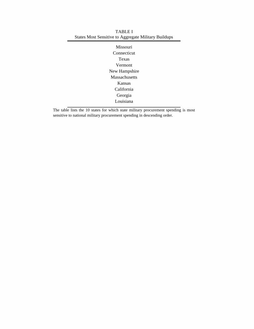
TABLE IStates Most Sensitive to Aggregate Military Buildups

MissouriConnecticut

TexasVermont

New HampshireMassachusetts

KansasCaliforniaGeorgia

Louisiana

The table lists the 10 states for which state military procurement spending is mostsensitive to national military procurement spending in descending order.

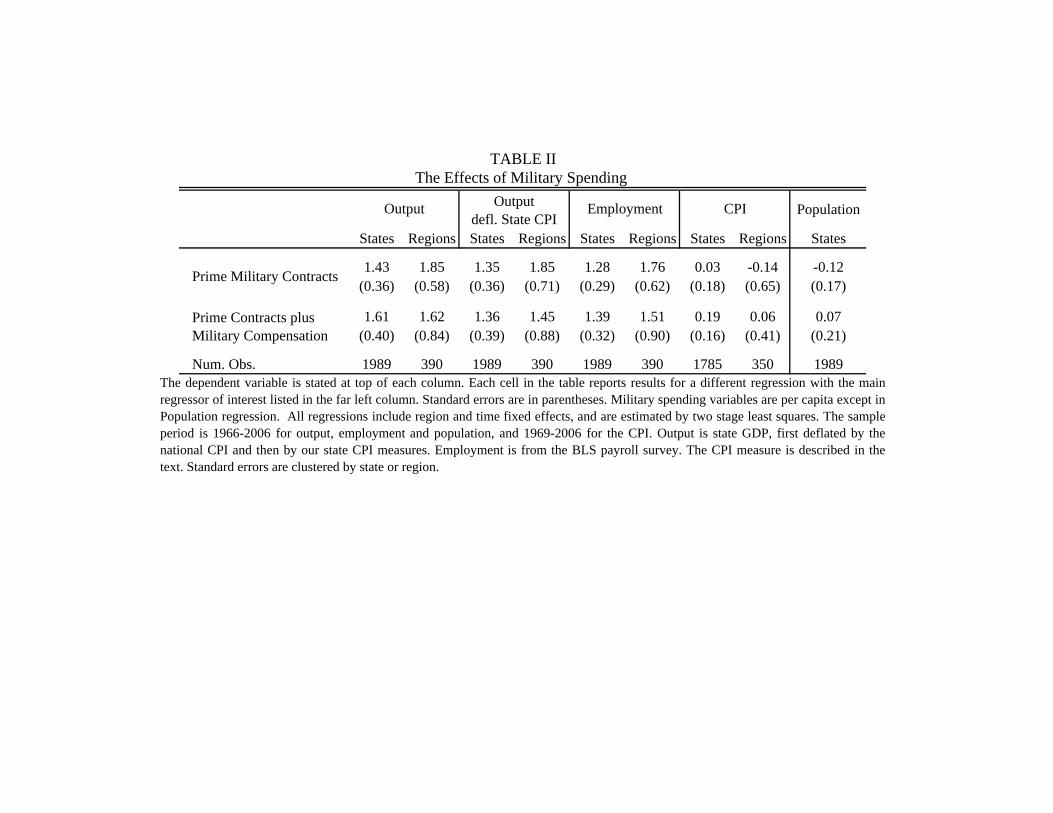
Population

States Regions States Regions States Regions States Regions States

1.43 1.85 1.35 1.85 1.28 1.76 0.03 -0.14 -0.12(0.36) (0.58) (0.36) (0.71) (0.29) (0.62) (0.18) (0.65) (0.17)

1.61 1.62 1.36 1.45 1.39 1.51 0.19 0.06 0.07(0.40) (0.84) (0.39) (0.88) (0.32) (0.90) (0.16) (0.41) (0.21)

Num. Obs. 1989 390 1989 390 1989 390 1785 350 1989

Prime Contracts plus Military Compensation

The dependent variable is stated at top of each column. Each cell in the table reports results for a different regression with the mainregressor of interest listed in the far left column. Standard errors are in parentheses. Military spending variables are per capita except inPopulation regression. All regressions include region and time fixed effects, and are estimated by two stage least squares. The sampleperiod is 1966-2006 for output, employment and population, and 1969-2006 for the CPI. Output is state GDP, first deflated by thenational CPI and then by our state CPI measures. Employment is from the BLS payroll survey. The CPI measure is described in thetext. Standard errors are clustered by state or region.

TABLE IIThe Effects of Military Spending

Output Employment CPI

Prime Military Contracts

Output defl. State CPI

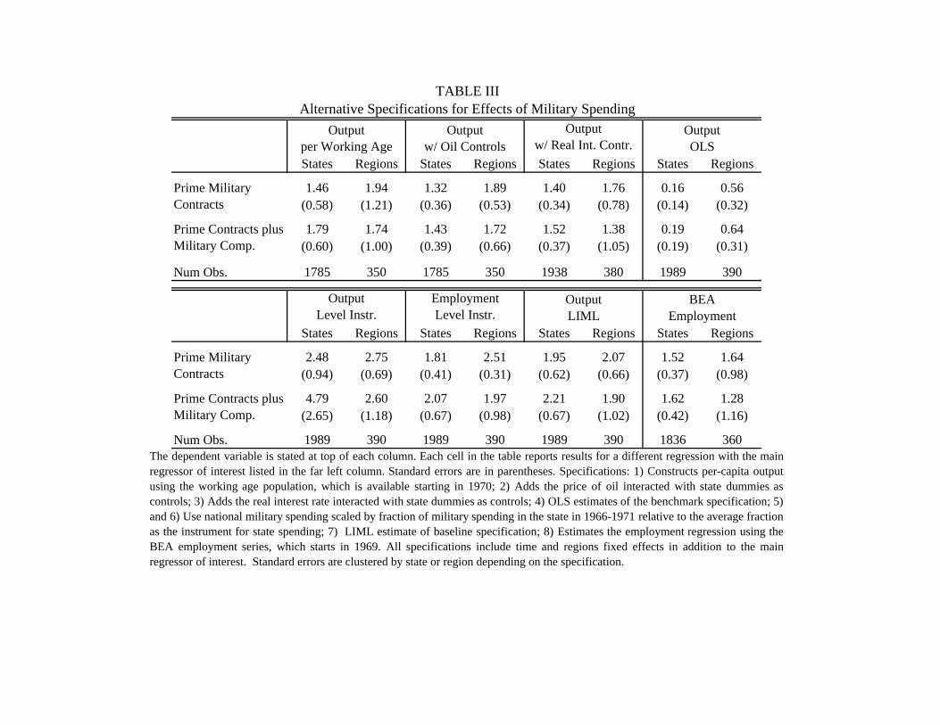
States Regions States Regions States Regions States Regions

1.46 1.94 1.32 1.89 1.40 1.76 0.16 0.56(0.58) (1.21) (0.36) (0.53) (0.34) (0.78) (0.14) (0.32)

1.79 1.74 1.43 1.72 1.52 1.38 0.19 0.64(0.60) (1.00) (0.39) (0.66) (0.37) (1.05) (0.19) (0.31)

Num Obs. 1785 350 1785 350 1938 380 1989 390

States Regions States Regions States Regions States Regions

2.48 2.75 1.81 2.51 1.95 2.07 1.52 1.64(0.94) (0.69) (0.41) (0.31) (0.62) (0.66) (0.37) (0.98)

4.79 2.60 2.07 1.97 2.21 1.90 1.62 1.28(2.65) (1.18) (0.67) (0.98) (0.67) (1.02) (0.42) (1.16)

Num Obs. 1989 390 1989 390 1989 390 1836 360

Prime Military Contracts

Prime Contracts plus Military Comp.

Output w/ Real Int. Contr.

Employment Level Instr.

The dependent variable is stated at top of each column. Each cell in the table reports results for a different regression with the mainregressor of interest listed in the far left column. Standard errors are in parentheses. Specifications: 1) Constructs per-capita outputusing the working age population, which is available starting in 1970; 2) Adds the price of oil interacted with state dummies ascontrols; 3) Adds the real interest rate interacted with state dummies as controls; 4) OLS estimates of the benchmark specification; 5)and 6) Use national military spending scaled by fraction of military spending in the state in 1966-1971 relative to the average fractionas the instrument for state spending; 7) LIML estimate of baseline specification; 8) Estimates the employment regression using theBEA employment series, which starts in 1969. All specifications include time and regions fixed effects in addition to the mainregressor of interest. Standard errors are clustered by state or region depending on the specification.

TABLE IIIAlternative Specifications for Effects of Military Spending

Output w/ Oil Controls

Output per Working Age

BEA Employment

Output OLS

Output LIML

Output Level Instr.

Prime Military Contracts

Prime Contracts plus Military Comp.

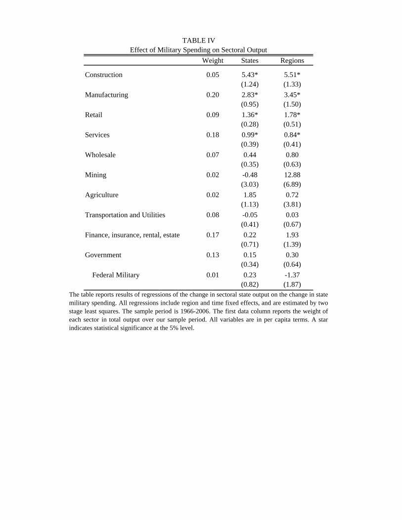
Weight States Regions

Construction 0.05 5.43* 5.51*(1.24) (1.33)

Manufacturing 0.20 2.83* 3.45*(0.95) (1.50)

Retail 0.09 1.36* 1.78*(0.28) (0.51)

Services 0.18 0.99* 0.84*(0.39) (0.41)

Wholesale 0.07 0.44 0.80(0.35) (0.63)

Mining 0.02 -0.48 12.88(3.03) (6.89)

Agriculture 0.02 1.85 0.72(1.13) (3.81)

Transportation and Utilities 0.08 -0.05 0.03(0.41) (0.67)

Finance, insurance, rental, estate 0.17 0.22 1.93(0.71) (1.39)

Government 0.13 0.15 0.30(0.34) (0.64)

Federal Military 0.01 0.23 -1.37(0.82) (1.87)

TABLE IVEffect of Military Spending on Sectoral Output

The table reports results of regressions of the change in sectoral state output on the change in statemilitary spending. All regressions include region and time fixed effects, and are estimated by twostage least squares. The sample period is 1966-2006. The first data column reports the weight ofeach sector in total output over our sample period. All variables are in per capita terms. A starindicates statistical significance at the 5% level.

States Regions States Regions

βh 3.54 3.27 1.85 2.20(1.51) (1.60) (0.85) (1.53)

βl ‐ βh -2.80 -1.85 -0.75 -0.57(1.49) (1.91) (0.89) (1.61)

Output EmploymentEffects of Military Spending in High Versus Low Unemployment Periods

TABLE V

The dependent variable is stated at top of each column. Standard errors are in parentheses. The tworegressors are 1) change in military spending and 2) change in military spending interacted with adummy indicating whether the national unemployment rate is below its median value over thesample period. This yields the effect of spending during high unemployment periods (βh) and thedifference between the effect of spending during low and high unemployment periods (βl - βh). Allregressions include region and time fixed effects, and are estimated by two stage least squares. Thesample period is 1966-2006. Output is state GDP. Employment is from the BLS payroll survey. Allvariables are per capita.

Closed Economy Agg. Multiplier

Open Economy Rel. Multiplier

Panel A: Separable PreferencesVolcker-Greenspan Monetary Policy 0.22 0.85Constant Real Rate 1.00 0.85Constant Nominal Rate -0.39 0.85Constant Nominal Rate (ρg=0.85) 1.70 0.90Flexible Prices 0.39 0.43

Panel B: GHH PreferencesVolcker-Greenspan Monetary Policy 0.15 1.48Constant Real Rate 7.00 1.48Constant Nominal Rate -0.64 1.48Constant Nominal Rate (ρg=0.50) 8.73 2.09Flexible Prices 0.00 0.30

TABLE VIGovernment Spending Multiplier in Business Cycle Models

The table reports the government spending multiplier for output deflated by the regional CPI for differentspecifications of the business cycle model presented in the text. Panel A presents results for the model withseparable preferences, while panel B presents results for the model with GHH preferences. The first threerows in each panel differ only in the monetary policy being assumed. The fourth row in each panel varies thepersistence of the government spending shock relative to the baseline parameter values. The fifth rowpresents results for a version of the model with flexible prices.

Output Employment CPI Inflation

No Capital 1.48 2.10 0.15w/ Capital, Baseline 1.10 0.79 0.10w/ Capital, High Labor Supply Elast. 1.47 1.44 0.02w/ Capital, Flexible Prices 0.45 0.23 0.30

Open Economy Relative Multipliers for Output, Employment and InflationTABLE VII

The table reports the open economy relative government spending multiplier for output, employmentand CPI inflation for the model with GHH preferences both excluding and including capital. Output isdeflated by the regional CPI. The first row presents results for the baseline specificaiton of the GHHmodel (same as in in table 5). The second row presents results for the baseline calibration of the modelwith capital. The third row presents results for the model with capital and with a labor supply elasticiyof 25. The last row presents results for the model with capital and flexible prices.

Figure I Prime Military Contract Spending as a Fraction of State GDP

0

0.01

0.02

0.03

0.04

0.05

0.06

0.07

0.08

1966 1970 1974 1978 1982 1986 1990 1994 1998 2002 2006

California

National

Illinois

Figure II Prime Military Contracts and Military Shipments

0

5

10

15

20

25

30

35

1966 1970 1974 1978 1982 1986 1990 1994 1998 2002 2006

Billion $ California

Prime Military Contracts

Military Shipments

012345678910

1966 1970 1974 1978 1982 1986 1990 1994 1998 2002 2006

Billion $ Conneticut

0

12

34

56

78

9

10

1966 1970 1974 1978 1982 1986 1990 1994 1998 2002 2006

Billion $ Massachusets

0

5

10

15

20

25

30

1966 1970 1974 1978 1982 1986 1990 1994 1998 2002 2006

Billion $ Texas

FIGURE III Quantiles of Change in Output Versus Predicted Change in Military Spending

The figure shows averages of changes in output and predicted military spending (based on our first-stage regression), grouped by 30 quantiles of the predicted military spending variable. Both variables are demeaned by year and state fixed effects.

-0.02

-0.01

0

0.01

0.02

-0.01 -0.005 0 0.005 0.01

Figure IV Prices and Real Interest Rates after a Government Spending Shock

The figure plots the relative price level and the relative real interest rate in the two regions for the model with separable preferences after a positive government spending shock to the home region.

-0.10

-0.05

0.00

0.05

0.10

0.15

0.20

0.25

0 5 10 15 20 25 30 35 40 45 50 55 60 65 70 75 80

Price LevelReal Interest Rate

Figure V Consumption and Real Interest Rate after a Government Spending Shock

The figure plots the relative consumption and the relative real interest rate in the two regions for the model with separable preferences after a positive government spending shock to the home region.

-0.25

-0.20

-0.15

-0.10

-0.05

0.00

0.05

0 5 10 15 20 25 30 35 40 45 50 55 60 65 70 75 80

ConsumptionReal Interest Rate

Figure VI Output and Consumption after a Government Spending Shock in GHH Model

The figure plots the relative output and consumption in the two regions for the model with GHH preferences after a positive government spending shock to the home region.

-0.50

0.00

0.50

1.00

1.50

2.00

2.50

0 5 10 15 20 25 30 35 40

Output

Consumption

Government Spending