Monetary and Fiscal Policy in the European Monetary Union · Monetary and Fiscal Policy in the European Monetary Union Jürgen von Hagen and Matthias Brückner ... monetary and fiscal

123

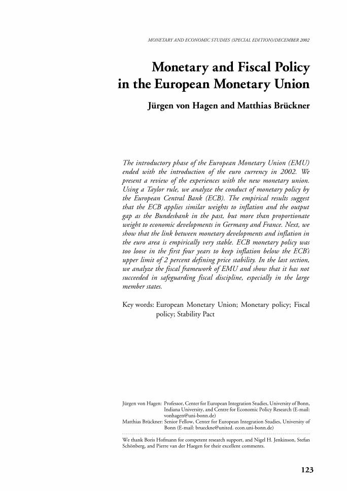
Monetary and Fiscal Policyin the European Monetary Union

Jürgen von Hagen and Matthias Brückner

MONETARY AND ECONOMIC STUDIES (SPECIAL EDITION)/DECEMBER 2002

The introductory phase of the European Monetary Union (EMU)ended with the introduction of the euro currency in 2002. We present a review of the experiences with the new monetary union.Using a Taylor rule, we analyze the conduct of monetary policy bythe European Central Bank (ECB). The empirical results suggestthat the ECB applies similar weights to inflation and the outputgap as the Bundesbank in the past, but more than proportionateweight to economic developments in Germany and France. Next, weshow that the link between monetary developments and inflation inthe euro area is empirically very stable. ECB monetary policy wastoo loose in the first four years to keep inflation below the ECB’supper limit of 2 percent defining price stability. In the last section,we analyze the fiscal framework of EMU and show that it has not succeeded in safeguarding fiscal discipline, especially in the largemember states.

Key words: European Monetary Union; Monetary policy; Fiscalpolicy; Stability Pact

Jürgen von Hagen: Professor, Center for European Integration Studies, University of Bonn,Indiana University, and Centre for Economic Policy Research (E-mail:[email protected])

Matthias Brückner: Senior Fellow, Center for European Integration Studies, University ofBonn (E-mail: brueckne@united. econ.uni-bonn.de)

We thank Boris Hofmann for competent research support, and Nigel H. Jenkinson, StefanSchönberg, and Pierre van der Haegen for their excellent comments.

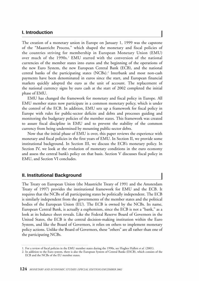
I. Introduction

The creation of a monetary union in Europe on January 1, 1999 was the capstone of the “Maastricht Process,” which shaped the monetary and fiscal policies of the countries striving for membership in European Monetary Union (EMU) over much of the 1990s.1 EMU started with the conversion of the national currencies of the member states into euros and the beginning of the operations of the new Euro System, the new European Central Bank (ECB), and the national central banks of the participating states (NCBs).2 Interbank and most non-cash payments have been denominated in euros since the start, and European financial markets quickly adopted the euro as the unit of account. The replacement of the national currency signs by euro cash at the start of 2002 completed the initialphase of EMU.

EMU has changed the framework for monetary and fiscal policy in Europe. AllEMU member states now participate in a common monetary policy, which is underthe control of the ECB. In addition, EMU sets up a framework for fiscal policy inEurope with rules for public-sector deficits and debts and processes guiding andmonitoring the budgetary policies of the member states. This framework was createdto assure fiscal discipline in EMU and to prevent the stability of the common currency from being undermined by mounting public-sector debts.

Now that the initial phase of EMU is over, this paper reviews the experience withmonetary and fiscal policies in the first years of EMU. In Section II, we provide someinstitutional background. In Section III, we discuss the ECB’s monetary policy. InSection IV, we look at the evolution of monetary conditions in the euro economyand assess the central bank’s policy on that basis. Section V discusses fiscal policy inEMU, and Section VI concludes.

II. Institutional Background

The Treaty on European Union (the Maastricht Treaty of 1991 and the AmsterdamTreaty of 1997) provides the institutional framework for EMU and the ECB. Itrequires that the NCBs of all participating states be politically independent. The ECBis similarly independent from the governments of the member states and the politicalbodies of the European Union (EU). The ECB is owned by the NCBs. Its name,European Central Bank, is actually a euphemism, since the ECB is not a “bank,” as alook at its balance sheet reveals. Like the Federal Reserve Board of Governors in theUnited States, the ECB is the central decision-making institution within the EuroSystem, and like the Board of Governors, it relies on others to implement monetarypolicy actions. Unlike the Board of Governors, these “others” are all rather than one ofthe participating NCBs.

124 MONETARY AND ECONOMIC STUDIES (SPECIAL EDITION)/DECEMBER 2002

1. For a review of fiscal policies in the EMU member states during the 1990s, see Hughes Hallett et al. (2001).2. In addition to the Euro system, there is also the European System of Central Banks (ESCB), which consists of the

ECB and the NCBs of the EU member states.

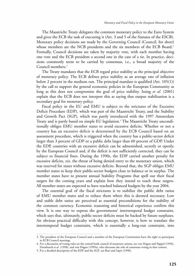
The Maastricht Treaty delegates the common monetary policy to the Euro Systemand gives the ECB the task of executing it (Art. 3 and 5 of the Statutes of the ESCB).Monetary policy decisions are made by the Governing Council (Council, for short)whose members are the NCB presidents and the six members of the ECB Board.3

Formally, Council decisions are taken by majority vote, with each member havingone vote and the ECB president a second one in the case of a tie. In practice, deci-sions commonly seem to be carried by consensus, i.e., a broad majority of theCouncil members.4

The Treaty mandates that the ECB regard price stability as the principal objectiveof monetary policy. The ECB defines price stability as an average rate of inflationbelow 2 percent in the medium run. The principal mandate is qualified (Art. 105(1))by the call to support the general economic policies in the European Community aslong as this does not compromise the goal of price stability. Issing et al. (2001)explain that the ECB does not interpret this as saying that output stabilization is asecondary goal for monetary policy.

Fiscal policy in the EU and EMU is subject to the strictures of the ExcessiveDeficit Procedure (EDP), which was part of the Maastricht Treaty, and the Stabilityand Growth Pact (SGP), which was partly introduced with the 1997 AmsterdamTreaty and is partly based on simple EU legislation.5 The Maastricht Treaty uncondi-tionally obliges EMU member states to avoid excessive deficits. Whether or not acountry has an excessive deficit is determined by the ECB Council based on anassessment procedure, which is triggered when the country has a public-sector deficitlarger than 3 percent of GDP or a public debt larger than 60 percent of GDP. Underthe EDP, countries with an excessive deficit can be admonished, secretly or openly, by the European Council and, if the deficit is not sufficiently corrected, they can besubject to financial fines. During the 1990s, the EDP carried another penalty forexcessive deficits, viz. the threat of being denied entry to the monetary union, whichwas reserved for states without excessive deficits. Beyond that, the SGP obliges EMUmember states to keep their public-sector budgets close to balance or in surplus. Themember states have to present annual Stability Programs that spell out their fiscal targets for the coming years and explain how they intend to reach these targets. All member states are expected to have reached balanced budgets by the year 2004.

The essential goal of the fiscal strictures is to stabilize the public debt ratios of EMU member states and to reduce them where this is deemed necessary. Low and stable debt ratios are perceived as essential preconditions for the stability of the common currency. Economic reasoning and historical experience confirm thisview. It is one way to express the governments’ intertemporal budget constraint,which says that, ultimately, public-sector deficits must be backed by future surpluses.An obvious practical difficulty with this concept, however, is how to translate theintertemporal budget constraint, which is essentially a long-run constraint, into

125

Monetary and Fiscal Policy in the European Monetary Union

3. The president of the European Council and a member of the European Commission have the right to participatein ECB Council meetings.

4. For a discussion of voting rules on the central bank council of monetary unions, see von Hagen and Süppel (1994),Dornbusch et al. (1998), and von Hagen (1999a), who discusses the role of consensus voting in that context.

5. For a detailed description of the EDP and the SGP, see Buti and Sapir (1998).

meaningful constraints on year-to-year fiscal policies (Perotti et al. [1998]). Focusingon the long run alone, the intertemporal budget constraint has no practical implica-tions for the short run, as governments can always promise future surpluses to excusecurrent deficits. The role of the annual deficit constraint in the EDP and SGP is tocreate the necessary link between the long and the short run. As we will see below,however, focusing too much on the annual deficit may undermine the credibility ofthe procedures, because the resulting constraints may keep countries from adoptingpolicies that would violate the deficit constraint initially but help reduce public debtin the medium and long run.

III. Monetary Policy in EMU

The ECB’s monetary policy evolves within a “two-pillar” strategy.6 The focal point of the first pillar is a “reference value” for the annual growth rate of a broad monetaryaggregate, M3. The reference value is derived from a simple quantity equation ofmoney. The second pillar consists of an analysis of short-run price movements usinga broad collection of data and a broad menu of alternative models. The ECB insiststhat the strategy is neither “monetary targeting” in a narrow sense of following a fixedmoney growth rule, nor “inflation targeting” in the sense of trying to achieve a giventarget rate of inflation over a specified time horizon. Instead, the two pillars serve toorganize monetary policy debates. The role of the first pillar is to focus attention onthe medium- and long-run consequences of monetary policy. In this regard, theECB’s strategy resembles the Bundesbank’s earlier practice of monetary targeting (vonHagen [1999b]). Short of an explicit intermediate target of monetary policy, theECB’s policy is best judged on the basis of its main policy instrument, the interestrate on its main repo operations.

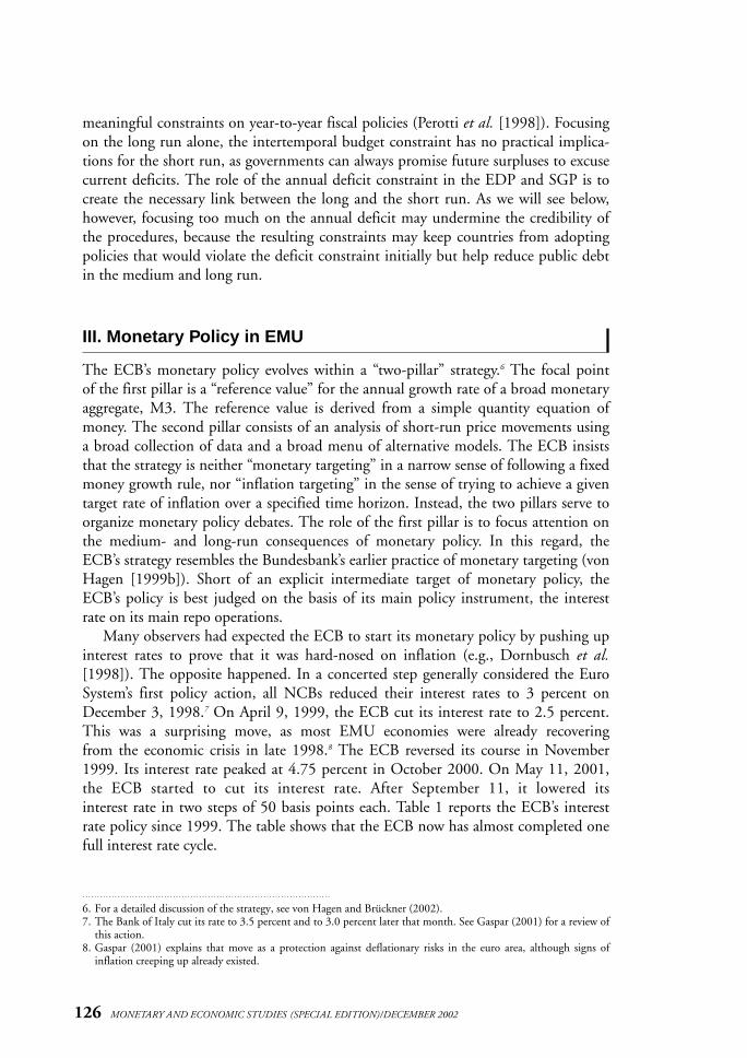
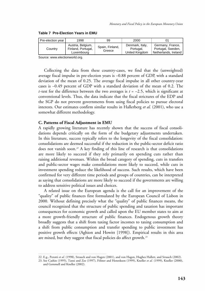
Many observers had expected the ECB to start its monetary policy by pushing upinterest rates to prove that it was hard-nosed on inflation (e.g., Dornbusch et al.[1998]). The opposite happened. In a concerted step generally considered the EuroSystem’s first policy action, all NCBs reduced their interest rates to 3 percent onDecember 3, 1998.7 On April 9, 1999, the ECB cut its interest rate to 2.5 percent.This was a surprising move, as most EMU economies were already recovering from the economic crisis in late 1998.8 The ECB reversed its course in November1999. Its interest rate peaked at 4.75 percent in October 2000. On May 11, 2001,the ECB started to cut its interest rate. After September 11, it lowered its interest rate in two steps of 50 basis points each. Table 1 reports the ECB’s interestrate policy since 1999. The table shows that the ECB now has almost completed onefull interest rate cycle.


6. For a detailed discussion of the strategy, see von Hagen and Brückner (2002).7. The Bank of Italy cut its rate to 3.5 percent and to 3.0 percent later that month. See Gaspar (2001) for a review of

this action.8. Gaspar (2001) explains that move as a protection against deflationary risks in the euro area, although signs of

inflation creeping up already existed.

Taylor rules have become a popular tool for describing and interpreting centralbank interest rate policies under very diverse circumstances. The simple Taylor rule (Taylor [1993]) found empirical support for the euro area already before the introduction of the euro (see, e.g., Gerlach and Schnabel [2000]). In view of that, it has received considerable attention as a benchmark for the ECB’s actual policy.9

Of course, we are fully aware of the fact that the ECB, like all central banks, has repeatedly affirmed that it does not follow a Taylor rule, and we do not want to suggestthat it blindly applies a technical relationship. Nevertheless, Taylor rules are a usefuldevice to summarize empirically observed patterns of central bank policy. Here, we follow the same approach. We base our exercise on the following specification:

it = 4.0 + 1.2(πt – πob) + 0.2yt , (1)

where it , πt , πob, and yt denote the main repo rate, the inflation rate, the inflationobjective, and the output gap, respectively. We set πob = 1.5 percent, the value implic-itly used by the ECB for its calculation of the reference value for M3, and assume anequilibrium interest rate of 4.0 percent, the sum of the ECB’s assumed long-run realGDP growth rate and the inflation objective. Since the measurement of the outputgap is particularly uncertain for the euro area due to data problems, we use a simpleaverage of the estimates provided by the Organisation for Economic Co-operationand Development (OECD [2002]), the International Monetary Fund (IMF [2002]),and the European Commission (EU [2001]) to obtain a robust measure.

The coefficients of the Taylor rule in equation (1) are chosen to resemble empiri-cal estimates for the Bundesbank prior to EMU, a plausible benchmark for the ECB(e.g., Faust et al. [2001]). This parameterization was also used in our previous study(von Hagen and Brückner [2002]), allowing for a simple robustness check of earlierresults. One advantage is that this parameterization yields a value of the Taylor rulefor the euro area of 3 percent in December 1998, which corresponds to the actualvalue at the start of EMU. We prefer to impose such a plausible parameterization toestimating it, because the short time span does not allow obtaining of estimates thatare robust against changes in the number of data points or changes in the series used

127


9. See Peersman and Smets (1999), Taylor (1998), Alesina et al. (2001), Faust et al. (2001), and von Hagen andBrückner (2002) as well as the financial press, e.g., Financial Times Deutschland.

Table 1 ECB Interest Rate Policy

Date Interest rate (percent) Date Interest rate (percent)

Jan. 1, 1999 3.00 Sep. 1, 2000 4.50

Apr. 9, 1999 2.50 Oct. 6, 2000 4.75

Nov. 5, 1999 3.00 May 11, 2001 4.50

Feb. 2, 2000 3.25 Aug. 31, 2001 4.25

Mar. 17, 2000 3.50 Sep. 18, 2001 3.75

Apr. 28, 2000 3.75 Nov. 9, 2001 3.25

June 9, 2000 4.25

Source: European Central Bank, Monthly Bulletin, various issues.

to obtain EMU-wide output gaps. In contrast to Faust et al. (2001), we concentrateon Taylor rules based on the current rather than on an expected future inflation rate. The main reason is that calculating expected inflation rates from the data would force us to shorten the sample. As we show below, this does not change theresults significantly.10

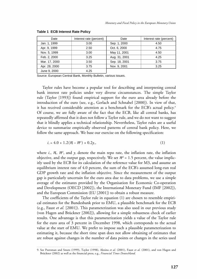
In Figure 1, we plot the Taylor rule from equation (1), labeled “euro,” togetherwith the ECB’s main policy instrument (“main rate”). The figure shows that the ECBkept its interest rate well below the benchmark from January 1999. If the benchmarkreflects what the Bundesbank would have done under similar circumstances, the figure suggests that the ECB’s monetary policy was consistently less tight thanBundesbank policy would have been. Note that the difference between the actual rateand the benchmark is not well explained by interest rate smoothing. With interestrate smoothing, the actual rate would adjust to the rate implied by the Taylor rulegradually, i.e.,

it = λit –1 + (1 – λ )(4.0 + 1.2(πt – πob) + 0.2yt), (2)

where λ > 0. Figure 1, however, shows that the actual rate and the rate calculatedfrom our Taylor rule move in opposite directions in at least two instances.


Figure 1 Taylor Rule and Interest Rates

7

6

5

4

3

2

1

0

Dec

. 199

8

Feb

. 199

9

Apr

. 199

9

June

199

9

Aug

. 199

9

Oct

. 199

9

Dec

. 199

9

Feb

. 200

0

Apr

. 200

0

June

200

0

Aug

. 200

0

Oct

. 200

0

Dec

. 200

0

Feb

. 200

1

Apr

. 200

1

June

200

1

Aug

. 200

1

Oct

. 200

1

Dec

. 200

1

Feb

. 200

2

Apr

. 200

2

June

200

2

Percent

Euro Main rate

10. The alternative way to proceed in the analysis would be to use EMU data for inflation and output gaps and the ECB’s interest rate and estimate the coefficients. Empirical studies doing this find a smaller coefficient on inflation and a larger coefficient on the output gap, suggesting that the ECB places more weight on outputstabilization and less on combating inflation than the Bundesbank did in the past (e.g., Neumann [2002]). Ourprocedure thus implicitly assumes that the ECB resembles the Bundesbank more strongly in its relative weightson output and inflation.

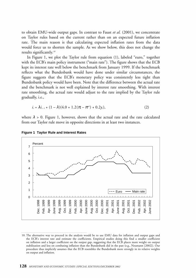
How can the difference between the actual rate and the benchmark be explained?It is sometimes argued that the ECB cares about (or should care about) core inflationinstead of headline inflation. In Figure 2, we show a Taylor rule with core inflationreplacing headline inflation. Core inflation is measured by excluding food and energyprices from the consumer price index (CPI) (“core 1”). This rule does not describethe ECB’s policy better than the benchmark. Since core inflation rose slowly butsteadily over most of the period under consideration, a Taylor rule based on coreinflation captures neither the tightening of monetary policy in 2000 nor the easing inlate 2001. A variant of this core inflation rule is to increase the weight on the outputgap. This follows the conjecture by Faust et al. (2001), namely, that the ECB placesmore weight on output stabilization than the Bundesbank did. Assuming a weight of 0.8 for output yields the rate labeled “core 2” in Figure 2. It describes the ECB’spolicy quite well until early 2000, even though it does not explain the low interestrates between April and October 1999. As the first Taylor rule based on core inflation, it does not capture the behavior of the interest rate from spring 2000onward. We conclude that the ECB does not aim at stabilizing core inflation. This isconsistent with recent results reported by Begg et al. (2002).11

129


11. In contrast, a former version of the CEPR Report, Alesina et al. (2001), claims that a core-inflation based Taylorrule performs well in describing ECB monetary policy.

Figure 2 Taylor Rules Based on Core Inflation

6

5

4

3

2

1

0

Dec

. 199

8

Feb

. 199

9

Apr

. 199

9

June

199

9

Aug

. 199

9

Oct

. 199

9

Dec

. 199

9

Feb

. 200

0

Apr

. 200

0

June

200

0

Aug

. 200

0

Oct

. 200

0

Dec

. 200

0

Feb

. 200

1

Apr

. 200

1

June

200

1

Aug

. 200

1

Oct

. 200

1

Dec

. 200

1

Feb

. 200

2

Apr

. 200

2

June

200

2

Percent

Core 1 Main rate Core 2

An alternative explanation is based on the decision-making structure in the ECB. If ECB Council decisions were taken by simple majority, the median NCB presidentwould have considerable influence on them. This is important, because national inflation rates in the EMU exhibited quite a large degree of cross-country variation

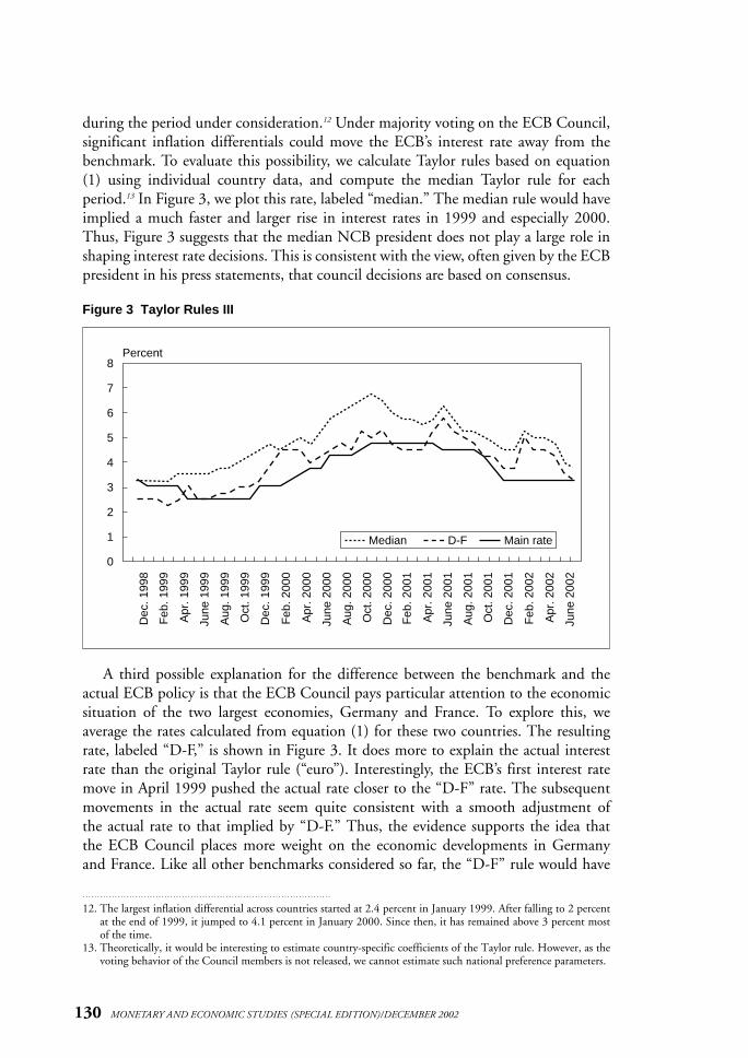
during the period under consideration.12 Under majority voting on the ECB Council,significant inflation differentials could move the ECB’s interest rate away from thebenchmark. To evaluate this possibility, we calculate Taylor rules based on equation (1) using individual country data, and compute the median Taylor rule for eachperiod.13 In Figure 3, we plot this rate, labeled “median.” The median rule would haveimplied a much faster and larger rise in interest rates in 1999 and especially 2000.Thus, Figure 3 suggests that the median NCB president does not play a large role inshaping interest rate decisions. This is consistent with the view, often given by the ECBpresident in his press statements, that council decisions are based on consensus.


12. The largest inflation differential across countries started at 2.4 percent in January 1999. After falling to 2 percentat the end of 1999, it jumped to 4.1 percent in January 2000. Since then, it has remained above 3 percent mostof the time.

13. Theoretically, it would be interesting to estimate country-specific coefficients of the Taylor rule. However, as thevoting behavior of the Council members is not released, we cannot estimate such national preference parameters.

Figure 3 Taylor Rules III

8

7

6

5

4

3

2

1

0

Dec

. 199

8

Feb

. 199

9

Apr

. 199

9

June

199

9

Aug

. 199

9

Oct

. 199

9

Dec

. 199

9

Feb

. 200

0

Apr

. 200

0

June

200

0

Aug

. 200

0

Oct

. 200

0

Dec

. 200

0

Feb

. 200

1

Apr

. 200

1

June

200

1

Aug

. 200

1

Oct

. 200

1

Dec

. 200

1

Feb

. 200

2

Apr

. 200

2

June

200

2

Median D-F Main rate

Percent

A third possible explanation for the difference between the benchmark and theactual ECB policy is that the ECB Council pays particular attention to the economicsituation of the two largest economies, Germany and France. To explore this, weaverage the rates calculated from equation (1) for these two countries. The resultingrate, labeled “D-F,” is shown in Figure 3. It does more to explain the actual interestrate than the original Taylor rule (“euro”). Interestingly, the ECB’s first interest ratemove in April 1999 pushed the actual rate closer to the “D-F” rate. The subsequentmovements in the actual rate seem quite consistent with a smooth adjustment of the actual rate to that implied by “D-F.” Thus, the evidence supports the idea thatthe ECB Council places more weight on the economic developments in Germanyand France. Like all other benchmarks considered so far, the “D-F” rule would have

called for a tighter monetary policy in the beginning of 2002 due to the jump in the inflation rate. However, most recently actual interest rates and the “D-F” rule coincide again.

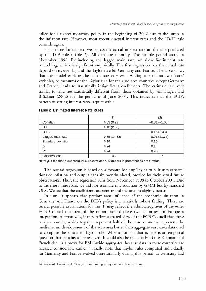
For a more formal test, we regress the actual interest rate on the rate predicted by the D-F rule (Table 2). All data are monthly. The sample period starts inNovember 1998. By including the lagged main rate, we allow for interest ratesmoothing, which is significant empirically. The first regression has the actual ratedepend on its own lag and the Taylor rule for Germany and France. The table showsthat this model explains the actual rate very well. Adding one of our two “core” variables, or measures of the Taylor rule for the euro-area countries except Germanyand France, leads to statistically insignificant coefficients. The estimates are very similar to, and not statistically different from, those obtained by von Hagen andBrückner (2002) for the period until June 2001. This indicates that the ECB’s pattern of setting interest rates is quite stable.

131


14. We would like to thank Nigel Jenkinson for suggesting this possible explanation.

Table 2 Estimated Interest Rate Rules

(1) (2)

Constant 0.03 (0.22) –0.31 (–1.65)

D-F 0.13 (2.58)

D-F+6 0.15 (3.48)

Lagged main rate 0.85 (14.33) 0.91 (21.75)

Standard deviation 0.19 0.19

ρ 0.24 0.1

R2 0.94 0.95

Observations 43 37

Note: ρ is the first-order residual autocorrelation. Numbers in parentheses are t -ratios.

The second regression is based on a forward-looking Taylor rule. It uses expecta-tions of inflation and output gaps six months ahead, proxied by their actual futureobservations. Thus, the regression runs from November 1998 to October 2001. Dueto the short time span, we did not estimate this equation by GMM but by standardOLS. We see that the coefficients are similar and the total fit slightly better.

In sum, it appears that predominant influence of the economic situation inGermany and France on the ECB’s policy is a relatively robust finding. There are several possible explanations for this. It may reflect the acknowledgment of the otherECB Council members of the importance of these two countries for European integration. Alternatively, it may reflect a shared view of the ECB Council that thesetwo economies, which together represent half of the euro economy, represent themedium-run developments of the euro area better than aggregate euro-area data usedto compute the euro-area Taylor rule. Whether or not that is true is an empiricalquestion that remains to be resolved. It could also be that the ECB uses German andFrench data as a proxy for EMU-wide aggregates, because data in these countries arereleased considerably earlier.14 Finally, note that Taylor rules computed individuallyfor Germany and France evolved quite similarly during this period, as Germany had

lower inflation rates but also a lower output gap than France. It remains an interest-ing question how ECB monetary policy might react when the German and theFrench economies call for interest rates moving in opposite directions.

IV. Monetary Relations in the Euro Area

In this section, we review the development of the relationship between money andprices in the euro area. First, we look at broad money and inflation since November1998 onward. Next, we estimate a long-run money demand function and use it todevelop a model for the long-run equilibrium price level. We then show that thismodel has considerable predictive power for price level movements in the euro area.

A. Monetary Developments and InflationMeasuring money growth is a difficult issue in EMU. The ECB’s key monetaryaggregate, M3, consists of cash, overnight deposits, deposits with fixed maturities ofup to two years, deposits with statutory maturity of up to three months, repurchaseagreements of financial institutions, money market fund shares, money market paper,bank certificates of deposit, and short-term obligations of maturities up to two years. Some of these elements are denominated in non-euro currencies, and others aretraded in secondary markets. These elements are subject to valuation changes as theirmarket prices change. In calculating the monthly growth rate of M3, the ECB purgesthe monetary data from these valuation changes. The ECB’s reasoning behind this is that changes in monetary assets caused by valuation changes rather than transactionsdo not cause portfolio adjustments and changes in private spending behavior (ECB [2001]), and therefore have no implications for inflation. The empiricalstrength of this conjecture, which is not in line with standard portfolio choice models, remains unclear.

A second issue is that the ECB’s original aggregate contained liabilities of euro-area financial institutions against non-banks residing outside the euro area.Noting that these liabilities were growing relatively fast from January 2000 onward,and very much so in early 2001, the ECB decided to redefine its aggregate excludingall liabilities against non-euro area residents. This introduces a potential measure-ment bias, however, as the relevant liabilities are not statistically measured in all euro-area countries. Unfortunately, the ECB has suppressed the publication of theearlier series, so that an assessment of its claim that this is a more relevant measure of “money” is impossible.

In Figure 4, we plot three measures of annual M3 growth rates. All three areadjusted for the reference value of 4.5 percent. Following ECB practice, they are calculated as centered three-month moving averages. The line labeled “ECB index” isthe ECB’s official money growth statistic. It shows money growth being roughly inline with the reference value at the start of EMU. The official money growth rate rosecontinually from the start of EMU to peak at about 2 percentage points above thereference value in April 2000. This confirms our earlier impression of a monetarypolicy stance that was too easy during 1999 and 2000. The official growth rate fell


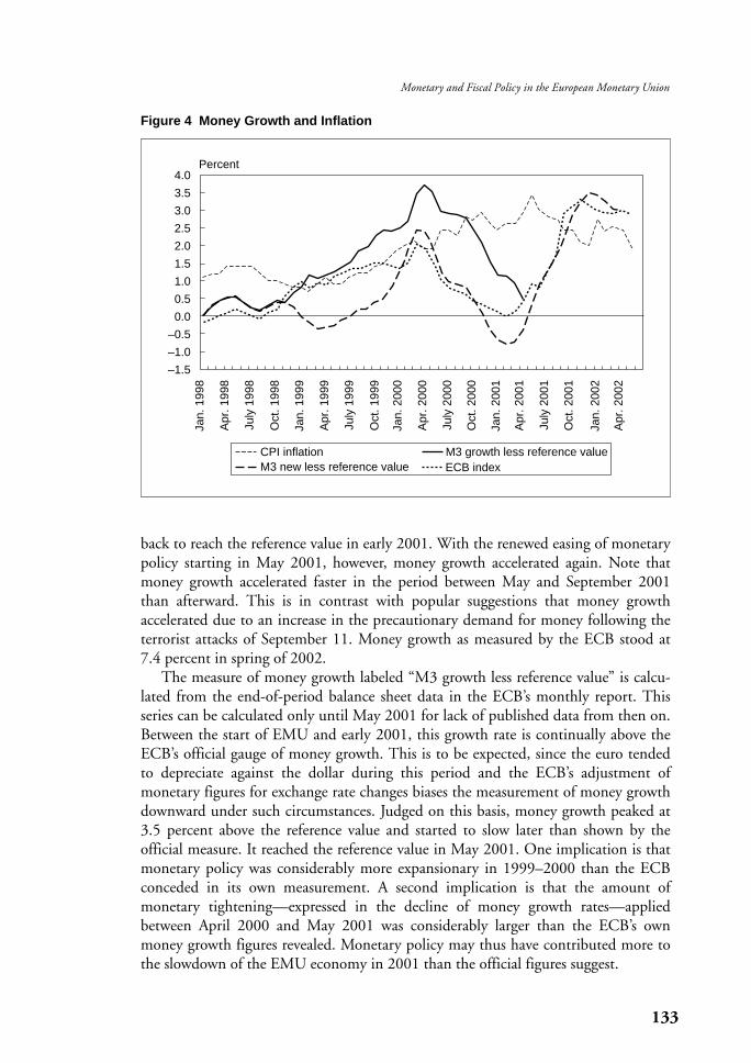
back to reach the reference value in early 2001. With the renewed easing of monetarypolicy starting in May 2001, however, money growth accelerated again. Note thatmoney growth accelerated faster in the period between May and September 2001than afterward. This is in contrast with popular suggestions that money growth accelerated due to an increase in the precautionary demand for money following theterrorist attacks of September 11. Money growth as measured by the ECB stood at7.4 percent in spring of 2002.

The measure of money growth labeled “M3 growth less reference value” is calcu-lated from the end-of-period balance sheet data in the ECB’s monthly report. Thisseries can be calculated only until May 2001 for lack of published data from then on.Between the start of EMU and early 2001, this growth rate is continually above theECB’s official gauge of money growth. This is to be expected, since the euro tendedto depreciate against the dollar during this period and the ECB’s adjustment of monetary figures for exchange rate changes biases the measurement of money growthdownward under such circumstances. Judged on this basis, money growth peaked at3.5 percent above the reference value and started to slow later than shown by the official measure. It reached the reference value in May 2001. One implication is thatmonetary policy was considerably more expansionary in 1999–2000 than the ECBconceded in its own measurement. A second implication is that the amount of monetary tightening—expressed in the decline of money growth rates—appliedbetween April 2000 and May 2001 was considerably larger than the ECB’s ownmoney growth figures revealed. Monetary policy may thus have contributed more tothe slowdown of the EMU economy in 2001 than the official figures suggest.

133


Figure 4 Money Growth and Inflation

4.0

3.5

3.0

2.5

2.0

1.5

1.0

0.5

0.0

–0.5

–1.0

–1.5

Jan.

199

8

Apr

. 199

8

July

199

8

Oct

. 199

8

Jan.

199

9

Apr

. 199

9

July

199

9

Oct

. 199

9

Jan.

200

0

Apr

. 200

0

July

200

0

Oct

. 200

0

Jan.

200

1

Apr

. 200

1

July

200

1

Oct

. 200

1

Jan.

200

2

Apr

. 200

2

CPI inflationM3 new less reference value

M3 growth less reference valueECB index

Percent

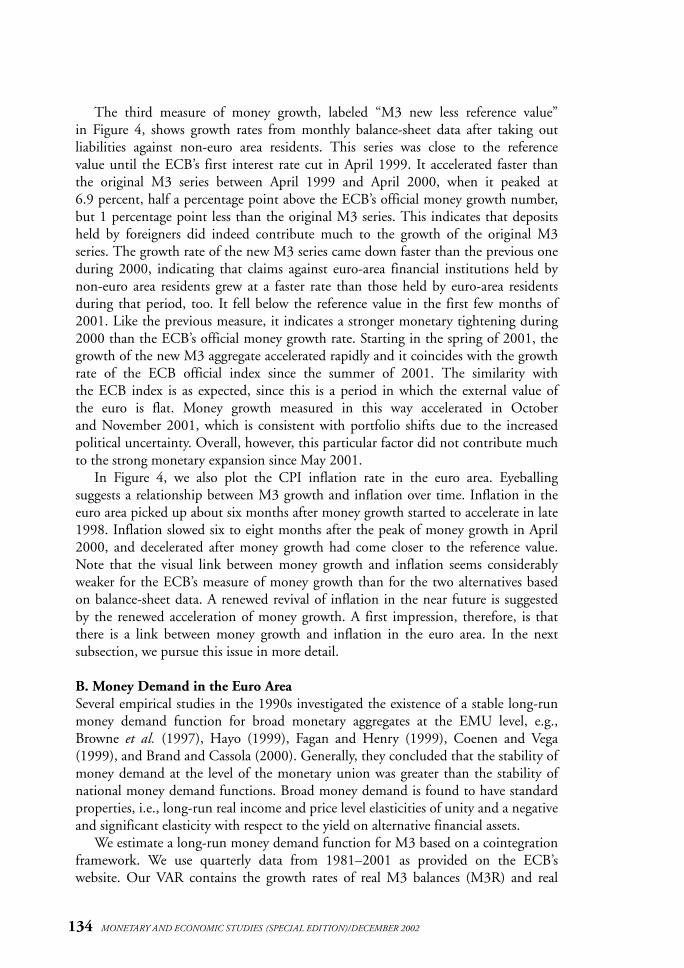
The third measure of money growth, labeled “M3 new less reference value” in Figure 4, shows growth rates from monthly balance-sheet data after taking out liabilities against non-euro area residents. This series was close to the reference value until the ECB’s first interest rate cut in April 1999. It accelerated faster than the original M3 series between April 1999 and April 2000, when it peaked at 6.9 percent, half a percentage point above the ECB’s official money growth number,but 1 percentage point less than the original M3 series. This indicates that depositsheld by foreigners did indeed contribute much to the growth of the original M3series. The growth rate of the new M3 series came down faster than the previous oneduring 2000, indicating that claims against euro-area financial institutions held bynon-euro area residents grew at a faster rate than those held by euro-area residentsduring that period, too. It fell below the reference value in the first few months of2001. Like the previous measure, it indicates a stronger monetary tightening during2000 than the ECB’s official money growth rate. Starting in the spring of 2001, thegrowth of the new M3 aggregate accelerated rapidly and it coincides with the growthrate of the ECB official index since the summer of 2001. The similarity with the ECB index is as expected, since this is a period in which the external value of the euro is flat. Money growth measured in this way accelerated in October and November 2001, which is consistent with portfolio shifts due to the increasedpolitical uncertainty. Overall, however, this particular factor did not contribute muchto the strong monetary expansion since May 2001.

In Figure 4, we also plot the CPI inflation rate in the euro area. Eyeballing suggests a relationship between M3 growth and inflation over time. Inflation in theeuro area picked up about six months after money growth started to accelerate in late1998. Inflation slowed six to eight months after the peak of money growth in April2000, and decelerated after money growth had come closer to the reference value.Note that the visual link between money growth and inflation seems considerablyweaker for the ECB’s measure of money growth than for the two alternatives basedon balance-sheet data. A renewed revival of inflation in the near future is suggestedby the renewed acceleration of money growth. A first impression, therefore, is thatthere is a link between money growth and inflation in the euro area. In the next subsection, we pursue this issue in more detail.

B. Money Demand in the Euro AreaSeveral empirical studies in the 1990s investigated the existence of a stable long-runmoney demand function for broad monetary aggregates at the EMU level, e.g.,Browne et al. (1997), Hayo (1999), Fagan and Henry (1999), Coenen and Vega(1999), and Brand and Cassola (2000). Generally, they concluded that the stability ofmoney demand at the level of the monetary union was greater than the stability ofnational money demand functions. Broad money demand is found to have standardproperties, i.e., long-run real income and price level elasticities of unity and a negativeand significant elasticity with respect to the yield on alternative financial assets.

We estimate a long-run money demand function for M3 based on a cointegrationframework. We use quarterly data from 1981–2001 as provided on the ECB’s website. Our VAR contains the growth rates of real M3 balances (M3R) and real


GDP (Y ) and the yield on 10-year government bonds (i ) in the euro area. Real M3is calculated using the seasonally adjusted CPI for the euro area. We also include a dummy variable (D90), which is zero before the third quarter of 1990 and onethereafter and which accounts for the level effects of German unification on moneyand income. The VAR system has one lag for each variable, and the error correctionterm (ECT) from the cointegrating relationship. The cointegration rank test and themaximum eigenvalue test both indicate the existence of at most one cointegratingrelationship in these data. A maximum likelihood test for the restriction implied byusing real M3 balances does not reject the hypothesis. Estimation yields the systemreported in Table 3. The ECT is estimated as

ECT = 3.9 + ln(M3R)t – lnYt + 0.037it . (3)

135


Table 3 VAR Estimates

Dependent Regressorvariable ∆M3R ∆Y ∆i ECT C D90 R2

∆M3R 0.26 0.14 –0.0001 –0.03 0.006 0.023 0.38(0.10) (0.11) (0.002) (0.01) (0.0013) (0.005)

∆Y 0.14 –0.14 0.004 –0.04 0.008 0.005 0.19(0.10) (0.12) (0.002) (0.01) (0.001) (0.005)

∆i 2.50 9.10 0.48 –1.16 –0.14 0.18 0.33(6.48) (7.48) (0.10) (0.79) (0.08) (0.52)

Note: Numbers in parentheses are standard errors.

15. P * is only a proxy, since the level of output might differ in the hypothetical equilibrium.

The standard error of the coefficient on the interest rate in the regression fromwhich it is derived is 0.004. The hypothesis of a unit long-run income elasticity ofreal money demand is not rejected. The estimated relationship can be interpreted as amoney demand function. The VAR estimates indicate that real money adjusts nega-tively to a gap between actual and long-run equilibrium balances. This supports theinterpretation of the model as a long-run money demand function. The estimate ispractically identical with that obtained by Hayo et al. (2000), who use data coveringthe period from 1981 to 1999. Our results thus confirm the impression that thelong-run money demand function of the euro area is stable. Note also that the veloc-ity of M3 implied by our long-run money demand function exhibits no exogenoustrend, and including a trend in our model does not improve the estimate. This is incontrast with the ECB’s claim that M3 velocity has a negative trend. That spurioustrend is most likely a result of the decline in long-run interest rates over the sampleperiod. Since the ECB adjusts its reference value for M3 growth for the supposedvelocity trend, the reference value is biased toward too-high money growth.

For a systematic analysis of the relationship between money and inflation, weapply the concept of an equilibrium price level (von Hagen [1995]) or P*-model(Hallman et al. [1991]) for the euro area. We solve the money demand function forthe equilibrium price level, pt*, that would result approximately if all prices adjustedimmediately to current output, money, and interest rates in each period.15

pt* = m t – y rt + 0.037it . (4)

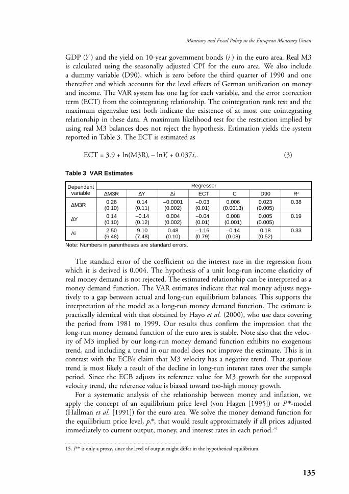
The equilibrium price level approach holds that the actual price level adjusts gradually to P* over time. Specifically, the rate of inflation follows the gap between theequilibrium price level and the actual price level with a lag. To test this hypothesis, weestimate a model explaining the annualized quarterly change in the CPI price index byits own lag, the change in oil prices, and the lagged gap between the equilibrium andthe actual price level.

Column (1) of Table 4 shows the estimate of this model for the period from 1981to 1998, just before the start of EMU. The model fits the data very well. TheDurbin-Watson statistic indicates no residual autocorrelation. The estimates showthat a 1 percent increase in the gap between the equilibrium and the actual price levelresults in an increase in the quarterly inflation rate of 0.11 percent in the followingperiod. Since the lagged inflation rate is significantly positive in this regression, themodel implies that the increase in the price gap feeds into inflation in the followingperiods, too. CPI inflation also adjusts gradually to changes in oil prices. Column (2)of Table 4 shows the estimate for the same model, but extending the sample periodto the end of 2001. The parameters are very stable, suggesting that the relationshipdid not change with the beginning of EMU. Column (3) of Table 4 presents thesame estimate including the output gap as an additional regressor. It shows that theoutput gap has no additional explanatory power over and above the price gap. Insum, the estimates confirm the visual link between money growth and inflation suggested by Figure 4.


Table 4 A Model for the Euro-Area Inflation Rate

(1) (2) (3)

Time period 1981/III–1998/IV 1981/III–2001/IV 1981/III–2001/IV

Constant 1.890 1.890 1.920(0.48)0 (0.44)0 (0.45)0

∆Pt –10.610 0.600 0.600

(0.09)0 (0.08)0 (0.08)0

P*t –1 – Pt –10.110 0.090 0.090

(0.04)0 (0.03)0 (0.03)0

∆poil,t0.006 0.007 0.007

(0.002) (0.002) (0.002)

D90 –1.2100 –1.0300 –1.0700(0.39)0 (0.22)0 (0.32)0

YGAP — —0.140

(0.13)0

Adj. R2 0.850 0.810 0.820

DW 2.300 2.300 2.300

F-test (joint) 89.8000 81.2000 65.5000

Note: Standard errors in parentheses.

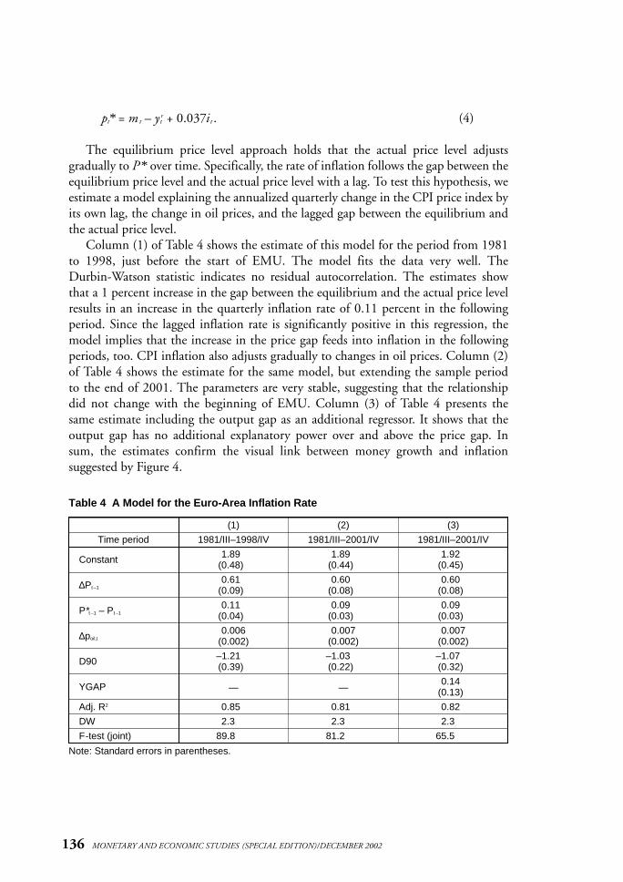
Figure 5 shows that actual, annualized quarterly change in the CPI (“CPI inflation”) together with its one-step-ahead forecast (“CPI inflation forecast”) derivedfrom this model for 1999–2001. In addition, the figure shows the estimated pricegap. The series shown in this figure are centered three-quarter moving averages. The figure indicates that the price gap rose quickly from the first quarter of 1999through the first quarter of 2000, reflecting the fact that monetary policy was overlyexpansionary in the first year of EMU. This confirms our earlier discussion.Reflecting the tightening of monetary policy, the price gap fell between mid-2000and early 2001, and returned to a rapid increase thereafter, Actual and predictedinflation tracks these movements with a lag and considerable smoothing. The empiri-cal analysis thus indicates that the rising inflation in the euro area in 1999–2000 canbe attributed in part at least to the ECB’s monetary policy. The temporary increase inactual inflation above the prediction of the model is consistent with the ECB’s viewthat non-monetary factors such as the spike in food prices following the outbreak ofhoof-and-mouth disease in Europe pushed prices upward during that period. Thewidening of the price gap since early 2001 signals that a further inflation potentialhas been building up in the euro area.16

137


16. Our model closely resembles the price-gap model proposed by Gerlach and Svensson (2001). An important difference, however, is that these authors include a measure of a moving trend inflation as an explanatory variable.This moving trend is calculated for each quarter as the slope of a Hodrick-Prescott filter for inflation. We find that,with our data, we can reproduce the Gerlach and Svensson estimates if we replace the D90 dummy by the inflationtrend. Essentially, the moving trend reproduces the shift in the relationship after 1990. Implicitly, their model thus explains only the deviation of the inflation rate from trend on the basis of the equilibrium price level.

Figure 5 Inflation and the Price Gap

3.5

3.0

2.5

2.0

1.5

1.0

0.5

0.0

8

7

6

5

4

3

2

1

0

–11999/I 1999/III 2000/I 2000/III 2001/I 2001/III

Inflation, percent Price gap

CPI inflation CPI inflation forecast Price gap

V. Fiscal Policy in EMU

In this section, we consider three issues. First, we review the fiscal consolidations of theEMU member states in the 1990s. We show that the consolidation experiences varygreatly for different member states. Second, we look at the fiscal performance since thestart of EMU. We show that the fiscal strictures did not prevent the reemergence of fiscal laxity. Furthermore, fiscal policy has been procyclical in the first years of EMUand has been driven by electoral considerations after the start of EMU. Third, we showthat there are very different patterns of fiscal adjustments. Countries that successfullyreduced their debt ratios did so relying predominantly on creating sufficient growth.The data suggest that fiscal policy contributed to that by restructuring spending awayfrom welfare spending and toward public investment. In contrast, countries that reliedpredominantly on reducing the growth of public debt did not achieve significantreductions in their debt burdens.

A. Fiscal Consolidations in the 1990s In 1992, the EU’s average debt ratio was almost 60 percent of GDP—hence the 60 percent limit foreseen in the Maastricht Treaty. This ratio climbed to almost 75 percent in 1997, the year whose fiscal data were the basis for the May 1998 decision on which countries could enter the monetary union. Since 1997, the averagedebt ratio has fallen to 62.8 percent. At first glance, these data suggest that the political process for fiscal consolidation started with the Maastricht Treaty was ratherunsuccessful until the start of EMU.

Several qualifications apply. First, it is important to note that the increase in theaverage debt ratio was driven mainly by the large debt expansions in five states:Germany (from 44 percent to 61 percent), France (from 40 percent to 56 percent),Spain (from 48 percent to 70 percent), Italy (from 109 percent to 124 percent), and the United Kingdom (from 42 percent to 55 percent). While Belgium andLuxembourg almost stabilized their debt ratios, the Netherlands and Ireland enjoyedfalling debt ratios during this period. The debt ratios of the other states were stabilized or fell after 1992.17

An institutional arrangement relying on enforcement by an external agent such asthe European Council and the European Commission presupposes that the internalpolitical processes of a country respond to external pressures. A country’s size is probably a first indicator of the importance of an external enforcement body. Smallcountries typically pay more attention to international organizations than largecountries do, and they do more so, the more they receive transfers from theseorganizations. This would suggest that the EDP works more powerfully in small EU states than in the large states. To assess this proposition, Table 5 reports thechanges in the debt-GDP ratios for states whose GDP in 1997 was at least 7 percentof EU GDP (large states Germany, Spain, France, Italy, and the United Kingdom),intermediate states, whose GDP was between 2 and 7 percent (Belgium, theNetherlands, Austria, and Sweden) and those whose GDP was less than 2 percent of


17. Austria’s and Finland’s debt ratios increased after 1992, but these countries were not bound by the EDP at the time.

EU GDP (small states Denmark, Greece, Ireland, Luxembourg, Portugal, andFinland). The combined GDP of the large states is 80 percent of EU GDP, that ofthe intermediate states 13 percent, and the small states have a combined GDP of7.7 percent of EU GDP. The table shows that, between 1992 and 1997, the averagedebt ratio of the small states increased by just 3.3 percent, much less than that of the large states, which rose by almost 19 percent. Between 1997 and 2001, the smallstates achieved a reduction in their debt ratios of almost 20 percent, much more thanthe 5.3 percent of the large states. Intermediate states behaved much like small states during this period.

This evidence suggests that the fiscal framework of EMU is more effective in thesmall than in the large states. But this means that the framework is most effectivewhere it matters the least. After all, a fiscal crisis in a small EMU member state wouldhardly pose a serious threat to the stability of the common currency. A fiscal crisis ina large state might do that, and the data suggest that the fiscal rules are much lesseffective in those member states. Recent anecdotal evidence confirms this impression.When the German government came under pressure in early 2002, an election yearin Germany, for not complying with its fiscal targets, the German finance ministerpromised to balance the budget by 2004. This is widely regarded as a commitmentthat Germany cannot achieve given economic and public revenue projections. Thus,the incident suggests that Germany expects to get away with making promises thatwill not be fulfilled. Shortly afterward, the newly appointed French governmentannounced that France plans to postpone balancing its budget until 2007, three yearslater than its commitments from the last two years had foreseen, and the Italian government stated a similar intention.

The second qualification is that the observation of fiscal consolidations in some EUstates during the 1990s does not mean that these can be attributed to the institutionalprovisions of the European Treaty. In fact, since most European countries experiencedsizeable fiscal expansions during the 1970s and 1980s, a period of consolidation couldbe expected in the 1990s in any case. In a study of European fiscal policy in the 1990s,Hughes Hallett et al. (2001) consider this argument in more detail. They estimateempirical models explaining the likelihood and duration of fiscal consolidations for allEU countries using data from the 1970s and 1980s. They then use the parameters estimated in this exercise to calculate the probability and the expected duration of fiscal consolidations using 1990s data. The results show that the empirical models predict almost all of the observed consolidations correctly. In other words, given thehigh debt ratios and the economic environment of the 1990s, the observed consolida-tions could be expected just by extrapolating the patterns of fiscal performance of EUstates in the 1970s and 1980s. This lends little force to the claim that the Maastricht

139


Table 5 Country Size and Government Debt in the 1990s

Change in debt ratio All EU countries Large states Intermediate Small states(percent) states

1992–97 15.8 18.8 4.1 3.3

1997–2001 –12.0 –5.3 –18.2 –19.8

Source: European Commission, Statistical Appendix of European Economy (Spring 2002).

process was important in making the EU countries embark on a process of fiscal consolidation.18 Hughes Hallett et al. (2001) find some weak evidence of a “Maastrichteffect” increasing the likelihood of fiscal consolidations in the years between 1992 and 1995. However, this effect only increased the likelihood of revenue-based con-solidations, which are less likely to last than expenditure-based consolidations. Thus, if the creation of the fiscal framework of the Maastricht Treaty had any positive effecton the governments’ willingness to undertake fiscal adjustments, the effect vanishedearly and its consequences were only short lived.

B. Fiscal Performance since the Start of EMUAfter 1997, the EU countries enjoyed a decline in their debt ratios. With the exception of 2001, the same years, however, were also a period of relatively stronggrowth in Europe. Since the fiscal performance is measured in terms of debt and surplus ratios relative to GDP, it is not clear to what extent the observed reductionsin government debt and deficit ratios can be attributed to government policy asopposed to windfall gains from strong economic growth. In this subsection, we assessthe recent performance, trying to separate policy from the effects of growth.

Separating the two requires making some assumptions about the contribution ofgrowth to the deficit ratio. To do this, we use a simple method of growth accounting.For each year, we estimate the change in the government surplus ratio due to economic growth and a “neutral” policy. Subtracting the two from the observedchange in the surplus ratio gives us an estimate of the active policy stance.19 Let theprimary surplus ratio, st , be

Rt – Gtst = ——— = (rt – gt), (5)Yt

where R denotes government revenues, G non-interest government spending, and YGDP. The change in this ratio over time then is

∆Rt – ∆Gt ∆Yt∆st = ———— – ——(rt – gt), (6)Yt –1 Yt –1

where r = R /Y, and g = G /Y. We define a “neutral” fiscal policy as one that keeps theaverage tax rate, r , and the ratio of government spending to trend GDP constant.With this definition, the contribution of the neutral policy to the change in the surplus ratio is

∆Yt ∆Y trend

∆stN = —–rt –1 – (——) gt –t . (7)

Yt –1 Y


18. An intriguing interpretation is that the governments wrote fiscal goals into the European Treaty that they werewilling to try to achieve anyway.

19. Alternatively, one might use the OECD’s cyclically adjusted budget balance and the OECD’s estimates of changesin structural balances. These estimates, however, are based on elasticities derived from past data and policies. If the1990s indeed brought a change in the fiscal policy regime in Europe, they could be quite misleading.

The contribution of the business cycle to the change in the surplus ratio is defined as

∆Yt ∆Y trend

∆stG = gt [ —– – (—–) ]. (8)

Yt –1 Y

This is the change that would occur in addition to the neutral change, if the government simply allowed economic growth above or below trend to change theexpenditure ratio. We estimate the trend growth rate as the average real growth rateduring the 1990s. We obtain the policy-induced change in the surplus ratio as

∆stP = ∆st – ∆st

N – ∆stG. (9)

This is our indicator of fiscal policy stance, since it measures the contribution ofany discretionary policy actions to observed changes in the surplus ratio. Table 6has our calculations for the years from 1998 to 2001. Columns labeled “observed”give the raw changes in surplus ratios, while columns labeled “policy” give the estimated policy stance from equation (9). Since the decision on EMU membershipwas taken in 1998 on the basis of fiscal data for 1997, 1998 was the first year after1992 in which the governments of the EMU member states were no longer under the risk of not making it into the monetary union due to excessively lax fiscal policies. In the table, a negative number indicates a fiscal expansion, a positive number a fiscal contraction.20

141


20. See Hughes Hallett et al. (2001) and Hallerberg et al. (2001) for similar calculations and results.

Table 6 Fiscal Policy Stance, 1998–2001

Country1998 99 2000 01

Observed Policy Observed Policy Observed Policy Observed Policy

Belgium 0.7 0.5 –0.3 –1.3 0.4 –1.5 –0.1 0.8Germany 0.5 0.4 0.6 0.7 0.0 –1.1 –1.5 –0.4Greece 1.1 0.2 0.9 –0.2 0.6 –1.1 0.1 –1.6Spain 0.1 –1.2 0.8 –0.4 0.4 –0.9 0.2 0.0France 0.2 –1.4 0.8 –0.3 0.2 –1.2 –0.1 –0.3Ireland 0.4 –1.0 –1.0 –3.8 1.9 –1.4 –3.4 –3.5Italy –1.5 –1.8 –0.2 –0.3 –0.3 –1.5 0.2 0.0Luxembourg 0.3 –0.5 0.6 –0.4 1.9 –0.4 –0.7 –1.0Netherlands 0.0 –1.4 0.8 0.0 0.5 –0.2 –1.8 –0.4Austria –0.6 –1.9 –0.1 –0.6 0.7 –0.0 1.4 2.6Portugal –0.5 –1.9 –0.2 –0.7 0.4 –0.1 –1.0 –0.2Finland 2.2 –1.3 0.1 –2.1 4.8 1.1 –2.2 –1.0Denmark 0.4 0.0 1.3 1.2 –1.1 –2.0 0.4 1.7Sweden 2.8 0.6 –1.4 –4.7 1.6 –0.6 0.3 0.8United Kingdom 2.5 1.9 0.1 0.2 0.3 –0.3 –1.0 –1.0EMU 0.0 –0.9 0.5 –0.1 0.0 –1.4 –0.4 –0.1


The table bears a number of interesting observations. The first is that the con-tribution of economic growth to the surplus ratios is large enough to hide the truepolicy stance in many cases. For example, France and Spain experienced risingobserved surplus ratios in 1998, while their policy stance was actually expansionary.On average, the EMU surplus ratio remained unchanged in 1998 and 2000, whilethe weighted average policy stance was negative. In 2001, the observed change in thesurplus ratio was negative in most countries and on average in the EMU, reflectingthe weak economic growth in that year.

The second, interesting observation is that “consolidation fatigue”—the loss ofpolitical interest in pursuing further consolidations—emerged in many countries inthe first year after the threat of not making it to EMU membership had disappeared.The (non-weighted) average fiscal impulse among the EMU member countries in1998 was –1.0 percent of GDP, with a standard deviation of the mean of 0.25. This compares to an average fiscal impulse in all other country-years of –0.5 percentof GDP with a standard deviation of 0.19. The t -test rejects the null hypothesis of equal means, which indicates that the 1998 fiscal impulses were significantly more expansionary among the EMU member states. Thus, these countries used thefirst opportunity to relax fiscal policies, even though 1998 was a year of relativelystrong economic growth. Interestingly, the countries that did not join EMU in 1999, Denmark, Greece, Sweden, and the United Kingdom all maintained tight orcontractionary fiscal policies in 1998.

The third observation from this table is a tendency for fiscal policy to be procyclical in the EMU.21 While the trend growth rate over the 1990s was 2 percent for the EMU, the actual growth rates were 2.9 percent, 2.6 percent, 3.4 percent, and 1.6 percent during 1998–2001. Thus, the two years with the strongest economicexpansions also saw the largest fiscal expansions, while the two years with less growthsaw a more or less neutral policy. Furthermore, Belgium, Austria, Denmark, andSweden all switched from a fiscal expansion in 2000 to a fiscal contraction in 2001,while Germany, Spain, France, Italy, and Portugal went from a fiscal expansion in2000 to a more or less neutral policy in 2001. Only Greece, Ireland, Luxembourg,the Netherlands, and Finland managed to achieve a countercyclical fiscal impulse inthe face of the incipient recession. The tendency to behave in a procyclical way mayindeed be a result of a fiscal policy that relaxes in times of strong economic growthand tightens in times of recession for fear of hitting the limits set by the EDP and theSGP. This tendency could be caused by the fact that the fiscal criteria of the EDP andthe SGP are related to raw surplus ratios unadjusted for cyclical effects.

A fourth observation emerges from considering the election dates in Europeancountries in recent years. If governments use fiscal policies to improve their chancesfor reelection, one should expect fiscal expansions in the year preceding the election.Table 7 indicates which years were pre-election years in which EU country. Here wecount both parliamentary and presidential elections where applicable.


21. Such a tendency was also noted by the European Commission (2000). Buti et al. (1998) show that procyclicalitywas already a property of EU fiscal policies in the 1980s.

Collecting the data from these country-cases, we find that the (unweighted) average fiscal impulse in pre-election years is –0.88 percent of GDP, with a standarddeviation of the mean of 0.25. The average fiscal impulse in all other country-yearcases is –0.49 percent of GDP with a standard deviation of the mean of 0.2. The t -test for the difference between the two averages is t = –2.5, which is significant atconventional levels. Thus, the data indicate that the fiscal strictures of the EDP andthe SGP do not prevent governments from using fiscal policies to pursue electoralinterests. Our estimates confirm similar results in Hallerberg et al. (2001), who use asomewhat different methodology.

C. Patterns of Fiscal Adjustment in EMUA rapidly growing literature has recently shown that the success of fiscal consoli-dations depends critically on the form of the budgetary adjustments undertaken. In this literature, success typically refers to the longevity of the fiscal consolidation:consolidations are deemed successful if the reduction in the public-sector deficit ratiodoes not vanish soon.22 A key finding of this line of research is that consolidations are more likely to succeed if they rely primarily on spending cuts rather than raising additional revenues. Within the broad category of spending, cuts in transfersand public-sector wages make consolidations more likely to succeed, while cuts ininvestment spending reduce the likelihood of success. Such results, which have beenconfirmed for very different time periods and groups of countries, can be interpretedas saying that consolidations are more likely to succeed if the governments are willingto address sensitive political issues and choices.

A related issue on the European agenda is the call for an improvement of the“quality” of public finances first formulated by the European Council of Lisbon in2000. Without defining precisely what the “quality” of public finances means, thecouncil recognized that the structure of public spending and taxation has importantconsequences for economic growth and called upon the EU member states to aim ata more growth-friendly structure of public finances. Endogenous growth theorybroadly suggests that a shift from taxing factor incomes to taxing consumption and a shift from public consumption and transfer spending to public investment has positive growth effects (Aghion and Howitt [1998]). Empirical results in this area are mixed, but they suggest that fiscal policies do affect growth.23

143


22. E.g., Perotti et al. (1998), Strauch and von Hagen (2001), and von Hagen, Hughes Hallett, and Strauch (2002).23. See Cashin (1995), Tanzi and Zee (1997), Fölster and Henrekson (1999), Kneller et al. (1999), Kneller (2000),

and Gemmell and Kneller (2002).

Table 7 Pre-Election Years in EMU

Pre-election year 1998 99 2000 01

Austria, Belgium, Spain, Finland, Denmark, Italy, Germany, France,Country Finland, Portugal, Greece Portugal, Portugal, Sweden,

Luxembourg United Kingdom Netherlands, Ireland

Source: www.electionworld.org.

Thus, the pattern of fiscal adjustment matters from a macroeconomic perspective.Subsequently, we characterize the fiscal policies of EMU member states to assess thestrength of this conjecture. We do this with a series of cross-section regressions focus-ing on the period since 1997. All data are taken from the Statistical Appendix ofEuropean Economy (Spring 2002), published by the European Commission. Whilethe cross-sections have obvious data limitations, the following bits of evidence add upto a picture that underscores the importance of the structure of fiscal adjustmentsmore generally.24

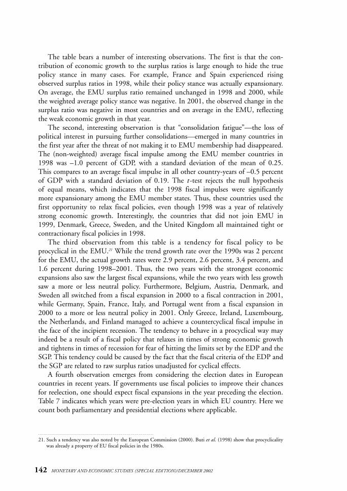
We start by noting that the fiscal rules of the EDP and SGP focus on a referencevalue for public debt relative to GDP. For countries with ratios exceeding the criticallimit, there are two ways to reduce it, by slowing the growth of nominal debt or byspeeding up the growth of GDP. Since inflation is no longer under the control ofdomestic monetary policy, the latter is equivalent to speeding up real GDP growth. Afirst question we look at considers the choice of the EMU governments betweenthese two options.

Let d = B /Y be the ratio of public debt, B , to GDP, Y. The relative contribution of growth in public debt and growth in real GDP to the change in this ratio in country i can be written as

1 + biCi = 100 (——– – 1), (10)1 + gi

where b is the growth rate of nominal debt and g is the growth rate of real GDP. If Ci > 0, the growth of public debt contributed more to the change in the debt ratiothan the growth of real GDP; otherwise, real GDP growth dominated.

Figure 6 plots Ci against the real growth rates of the EU countries for two timeperiods, 1992–97 and 1997–2001. Positive values on the x-axis indicate that thechange in the debt ratio during the period considered was due to growth rates ofpublic debt in excess of the growth rate of real GDP. This was true in almost all EUcountries in the first period. In contrast, public debt grew less than real GDP in allcountries since 1997. Significantly, the figure also shows a strong correlation betweenthe average real GDP growth rate over the post-1997 period and the relative contri-bution of GDP growth to the change in the debt ratio. Such a relationship did notexist in the first half of the 1990s.

Figure 7 plots the relative contributions of debt and real GDP growth against thechange in the debt ratio during the period under consideration. In the earlier period,when debt ratios increased, this was due to debt growing much faster than real GDP.In the later years, however, the pattern is reversed. Countries that achieved a largedecline in the debt ratio were countries that achieved high real GDP growth rates relative to the growth rate of debt over this period. Countries that achieved little real growth relative to debt growth also did not manage to reduce their debt ratios


24. To facilitate reading the following figures, note that an R-square of 0.20 in the following regressions correspondsto the 10 percent critical value, and an R-square of 0.26 to the 5 percent critical value of the F-distribution of atest for statistical significance.

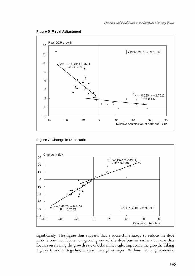
significantly. The figure thus suggests that a successful strategy to reduce the debtratio is one that focuses on growing out of the debt burden rather than one thatfocuses on slowing the growth rate of debt while neglecting economic growth. TakingFigures 6 and 7 together, a clear message emerges. Without reviving economic

145


Figure 6 Fiscal Adjustment

14

12

10

8

6

4

2

0

–2

y = –0.1553x + 1.9591R2 = 0.481

y = –0.0204x + 1.7212R2 = 0.1429

–60 –40 –20 0 20 40 60 80

Real GDP growth

Relative contribution of debt and GDP

1997–2001 1992–97

Figure 7 Change in Debt Ratio

–40 –20

30

20

10

0

–10

–20

–30

–40

–500 20 40 60 80–60

Change in B /Y

Relative contribution

1997–2001 1992–97

y = 0.4102x + 0.8444R2 = 0.6606

y = 0.6863x – 0.9152R2 = 0.7042

growth, a significant reduction in the debt burden is unlikely. Taking the two periodstogether, another message is that rising debt burdens come from a lack of controlover public-sector debt. But to reduce an excessive debt burden, controlling debt isonly a necessary condition. Without reviving economic growth, a significant declinein the debt burden seems unlikely. This suggests that the fiscal framework of EMU isill conceived. The focus on deficits and debt growth alone would be justified if EMUhad started in a period in which public debt burdens could be regarded as compatiblewith long-run equilibrium. Given that a reduction in the debt burden is necessaryparticularly in the large countries, the policy framework pays too little attention tothe role of economic growth in achieving sustainable public finances.

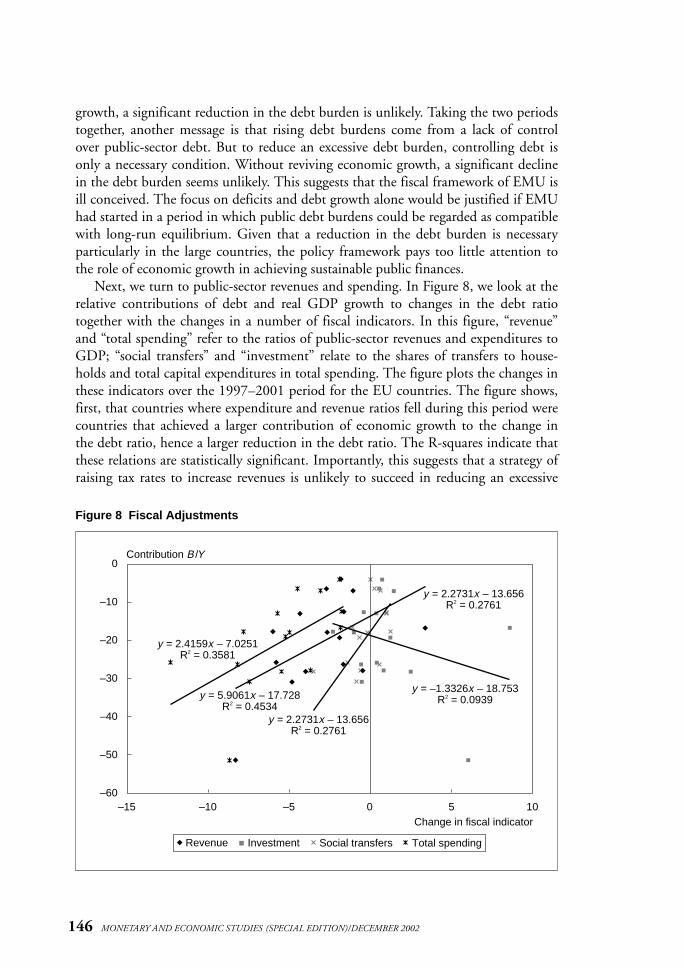
Next, we turn to public-sector revenues and spending. In Figure 8, we look at therelative contributions of debt and real GDP growth to changes in the debt ratiotogether with the changes in a number of fiscal indicators. In this figure, “revenue”and “total spending” refer to the ratios of public-sector revenues and expenditures toGDP; “social transfers” and “investment” relate to the shares of transfers to house-holds and total capital expenditures in total spending. The figure plots the changes inthese indicators over the 1997–2001 period for the EU countries. The figure shows,first, that countries where expenditure and revenue ratios fell during this period werecountries that achieved a larger contribution of economic growth to the change inthe debt ratio, hence a larger reduction in the debt ratio. The R-squares indicate thatthese relations are statistically significant. Importantly, this suggests that a strategy ofraising tax rates to increase revenues is unlikely to succeed in reducing an excessive


Figure 8 Fiscal Adjustments

0

–10

–20

–30

–40

–50

–60–15 –10 –5 0 5 10

Contribution B /Y

Change in fiscal indicator

Revenue Investment Social transfers Total spending

y = 5.9061x – 17.728R2 = 0.4534

y = 2.4159x – 7.0251R2 = 0.3581

y = 2.2731x – 13.656R2 = 0.2761

y = 2.2731x – 13.656R2 = 0.2761

y = –1.3326x – 18.753R2 = 0.0939

debt burden, because it slows economic growth. This is the German predicament offiscal policy after 1994. Repeated increases in tax rates only resulted in ever smallergrowth, with the result that Germany did not manage to approach budget balancenor reduce its debt burden sufficiently.25

The same figure also points to a critical role of investment spending and spendingon social transfers. Countries that increased the share of investment spending tendedto achieve a stronger contribution of GDP growth to the reduction in the debt burden, while the opposite is true for countries that increased the share of socialtransfers in total spending. We look at this issue in more detail below.

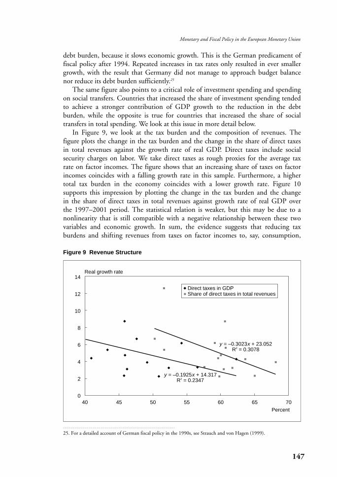
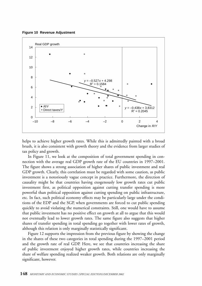
In Figure 9, we look at the tax burden and the composition of revenues. The figure plots the change in the tax burden and the change in the share of direct taxesin total revenues against the growth rate of real GDP. Direct taxes include social security charges on labor. We take direct taxes as rough proxies for the average taxrate on factor incomes. The figure shows that an increasing share of taxes on factorincomes coincides with a falling growth rate in this sample. Furthermore, a highertotal tax burden in the economy coincides with a lower growth rate. Figure 10supports this impression by plotting the change in the tax burden and the change in the share of direct taxes in total revenues against growth rate of real GDP over the 1997–2001 period. The statistical relation is weaker, but this may be due to anonlinearity that is still compatible with a negative relationship between these twovariables and economic growth. In sum, the evidence suggests that reducing tax burdens and shifting revenues from taxes on factor incomes to, say, consumption,

147


25. For a detailed account of German fiscal policy in the 1990s, see Strauch and von Hagen (1999).

Figure 9 Revenue Structure

14

12

10

8

6

4

2

0

y = –0.1925x + 14.317R2 = 0.2347

y = –0.3023x + 23.052R2 = 0.3078

Percent

Real growth rate

40 45 50 55 60 65 70

Direct taxes in GDPShare of direct taxes in total revenues

helps to achieve higher growth rates. While this is admittedly painted with a broadbrush, it is also consistent with growth theory and the evidence from larger studies oftax policy and growth.

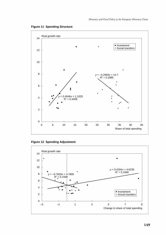
In Figure 11, we look at the composition of total government spending in con-nection with the average real GDP growth rate of the EU countries in 1997–2001.The figure shows a strong association of higher shares of public investment and realGDP growth. Clearly, this correlation must be regarded with some caution, as publicinvestment is a notoriously vague concept in practice. Furthermore, the direction ofcausality might be that countries having exogenously low growth rates cut publicinvestment first, as political opposition against cutting transfer spending is morepowerful than political opposition against cutting spending on public infrastructure,etc. In fact, such political economy effects may be particularly large under the condi-tions of the EDP and the SGP, when governments are forced to cut public spendingquickly to avoid violating the numerical constraints. Still, one would have to assumethat public investment has no positive effect on growth at all to argue that this wouldnot eventually lead to lower growth rates. The same figure also suggests that highershares of transfer spending in total spending go together with lower rates of growth,although this relation is only marginally statistically significant.

Figure 12 supports the impression from the previous figure by showing the changein the shares of these two categories in total spending during the 1997–2001 periodand the growth rate of real GDP. Here, we see that countries increasing the share of public investment enjoyed higher growth rates, while countries increasing the share of welfare spending realized weaker growth. Both relations are only marginallysignificant, however.


Figure 10 Revenue Adjustment

14

12

10

8

6

4

2

0–10 –8 –6 –4 –2 0 2 4

y = –0.527x + 4.298R2 = 0.1584

y = –0.438x + 3.8312R2 = 0.2045

Change in R/Y

Real GDP growth

R/YDirect taxes/Y

149


Figure 11 Spending Structure

14

12

10

8

6

4

2

00 5 10 15 20 25 30 35 40 45

Share of total spending

Real growth rate

y = –0.2959x + 14.7R2 = 0.1885

y = 0.4546x + 1.1525R2 = 0.4408

InvestmentSocial transfers

Figure 12 Spending Adjustment

14

12

10

8

6

4

2

0–3 –1 1 3 5 7 9

InvestmentSocial transfers

y = 0.4184x + 4.6235R2 = 0.1846

y = –0.7629x + 4.7805R2 = 0.1508

Real growth rate

Change in share of total spending

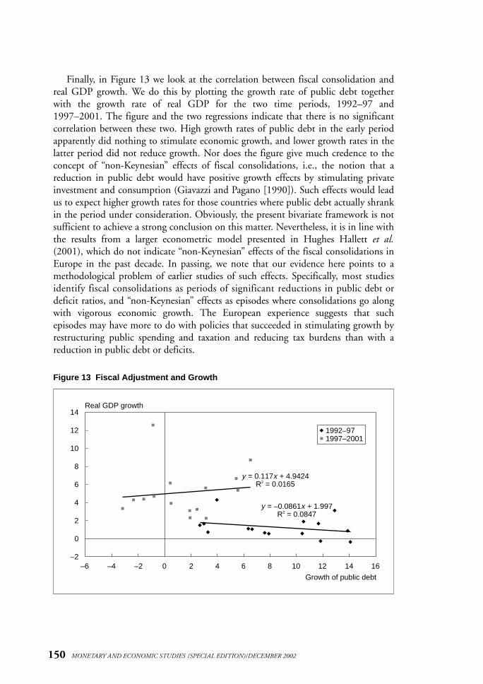
Finally, in Figure 13 we look at the correlation between fiscal consolidation andreal GDP growth. We do this by plotting the growth rate of public debt togetherwith the growth rate of real GDP for the two time periods, 1992–97 and1997–2001. The figure and the two regressions indicate that there is no significantcorrelation between these two. High growth rates of public debt in the early periodapparently did nothing to stimulate economic growth, and lower growth rates in thelatter period did not reduce growth. Nor does the figure give much credence to theconcept of “non-Keynesian” effects of fiscal consolidations, i.e., the notion that areduction in public debt would have positive growth effects by stimulating privateinvestment and consumption (Giavazzi and Pagano [1990]). Such effects would leadus to expect higher growth rates for those countries where public debt actually shrankin the period under consideration. Obviously, the present bivariate framework is notsufficient to achieve a strong conclusion on this matter. Nevertheless, it is in line withthe results from a larger econometric model presented in Hughes Hallett et al.(2001), which do not indicate “non-Keynesian” effects of the fiscal consolidations inEurope in the past decade. In passing, we note that our evidence here points to amethodological problem of earlier studies of such effects. Specifically, most studiesidentify fiscal consolidations as periods of significant reductions in public debt ordeficit ratios, and “non-Keynesian” effects as episodes where consolidations go alongwith vigorous economic growth. The European experience suggests that suchepisodes may have more to do with policies that succeeded in stimulating growth byrestructuring public spending and taxation and reducing tax burdens than with areduction in public debt or deficits.


Figure 13 Fiscal Adjustment and Growth

14

12

10

8

6

4

2

0

–2

Real GDP growth

Growth of public debt

–6 –4 –2 0 2 4 6 8 10 12 14 16

1992–971997–2001

y = 0.117x + 4.9424R2 = 0.0165

y = –0.0861x + 1.997R2 = 0.0847

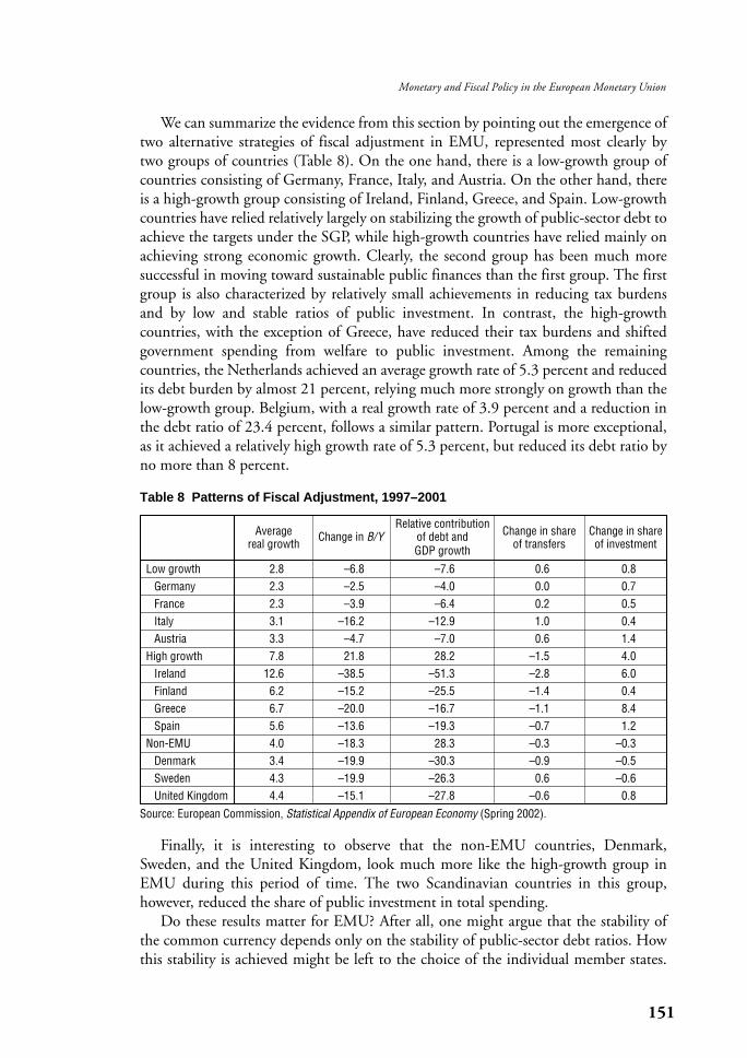
We can summarize the evidence from this section by pointing out the emergence oftwo alternative strategies of fiscal adjustment in EMU, represented most clearly by two groups of countries (Table 8). On the one hand, there is a low-growth group ofcountries consisting of Germany, France, Italy, and Austria. On the other hand, thereis a high-growth group consisting of Ireland, Finland, Greece, and Spain. Low-growthcountries have relied relatively largely on stabilizing the growth of public-sector debt toachieve the targets under the SGP, while high-growth countries have relied mainly onachieving strong economic growth. Clearly, the second group has been much moresuccessful in moving toward sustainable public finances than the first group. The firstgroup is also characterized by relatively small achievements in reducing tax burdensand by low and stable ratios of public investment. In contrast, the high-growth countries, with the exception of Greece, have reduced their tax burdens and shiftedgovernment spending from welfare to public investment. Among the remaining countries, the Netherlands achieved an average growth rate of 5.3 percent and reducedits debt burden by almost 21 percent, relying much more strongly on growth than thelow-growth group. Belgium, with a real growth rate of 3.9 percent and a reduction inthe debt ratio of 23.4 percent, follows a similar pattern. Portugal is more exceptional,as it achieved a relatively high growth rate of 5.3 percent, but reduced its debt ratio byno more than 8 percent.

151


Table 8 Patterns of Fiscal Adjustment, 1997–2001

AverageRelative contribution

Change in share Change in sharereal growth

Change in B/Y of debt and of transfers of investmentGDP growth

Low growth 2.8 –6.8 –7.6 0.6 0.8Germany 2.3 –2.5 –4.0 0.0 0.7France 2.3 –3.9 –6.4 0.2 0.5Italy 3.1 –16.2 –12.9 1.0 0.4Austria 3.3 –4.7 –7.0 0.6 1.4

High growth 7.8 21.8 28.2 –1.5 4.0Ireland 12.6 –38.5 –51.3 –2.8 6.0Finland 6.2 –15.2 –25.5 –1.4 0.4Greece 6.7 –20.0 –16.7 –1.1 8.4Spain 5.6 –13.6 –19.3 –0.7 1.2

Non-EMU 4.0 –18.3 28.3 –0.3 –0.3Denmark 3.4 –19.9 –30.3 –0.9 –0.5Sweden 4.3 –19.9 –26.3 0.6 –0.6United Kingdom 4.4 –15.1 –27.8 –0.6 0.8


Finally, it is interesting to observe that the non-EMU countries, Denmark,Sweden, and the United Kingdom, look much more like the high-growth group inEMU during this period of time. The two Scandinavian countries in this group,however, reduced the share of public investment in total spending.

Do these results matter for EMU? After all, one might argue that the stability ofthe common currency depends only on the stability of public-sector debt ratios. Howthis stability is achieved might be left to the choice of the individual member states.

The subsidiarity principle of the Treaty on European Union would then suggest thatthe EU should not interfere with these choices.

There are, however, at least two counterarguments to this. The first is that, ifEuropeans truly believe that public debt ratios must be low and sustainable, successin achieving this matters and is a valid concern for the EU. From this perspective, thecurrent fiscal framework is incomplete, because it does not give EMU member statesenough guidance for the choice of a successful fiscal strategy. Countries should beencouraged to adopt more growth-friendly policies by restructuring their tax andexpenditure systems.

Second, it is necessary to recognize that EMU did not start under conditions of along-run equilibrium as far as public finances are concerned. The low growth rates inGermany, France, and Italy in particular are the result of overregulated economiesplagued by high tax burdens and welfare systems that discourage employment. Thenarrow focus of the EDP and the SGP on annual deficits, however, may keep govern-ments from adopting reform policies that might result in larger deficits initiallybefore the desired growth and employment effects kick in. If so, the current design of the fiscal strictures risks keeping these countries in a state of low growth withinsufficient progress also as regards the reduction of debts and deficits. One may reasonably doubt that these large EMU states will continue to tolerate such a scenario, which is perceived as keeping them from adopting better economic policiesfor the sake of some fiscal targets imposed by the EU. The recent episodes involvingFrance and Germany clearly indicate that they will not. But if the outcome were thatthese countries simply began to ignore the goals of the EDP and the SGP, other stateswould follow and the fiscal framework of EMU would fall apart. A redesign of thisframework to account for the circumstances of the large states seems necessary toavoid such a development.

VI. Conclusions

In this paper, we have reviewed the monetary and fiscal policy experiences of the newmonetary union in Europe in its first few years. On the monetary side, the experienceis encouraging so far. Long-run monetary relations continue to be stable, and a focusof monetary policy on monetary developments is justified from the data. Still, 2002will be the third year in which inflation in the euro area is above the ECB’s 2 percentthreshold above which price stability does not prevail. This suggests that the ECB’spolicy was not sufficiently tight particularly in its first year, and that it should paymore attention to the developments under the “first pillar” of its strategy. In line with the ECB’s (and our) interpretation of its strategy, what we mean by this is notthat the ECB should blindly pursue a numerical target for M3 growth. It should,however, increase the weight of the implications for future inflation in its currentdecisions and reduce the weight given to the short-run considerations arising fromthe “second pillar.”

On the fiscal side, the picture is more mixed. The fiscal rules created by the EMUseem to be more effective where they matter less, namely in the small states. They did


not keep EMU states from relaxing fiscal discipline after the critical decision onEMU membership had been made, nor from using fiscal policies for electoral purposes. There is also a tendency for fiscal policy to be procyclical. Patterns of fiscal adjustment in recent years show that sustainable public finances need fiscalpolicies that stimulate and maintain sufficiently high long-run growth rates. The fiscal framework needs further improvements, taking this insight into account.

153


References

Aghion, Philippe, and Peter Howitt, Growth Theory. Boston: The MIT Press, 1998.Alesina, Alberto, Olivier Blanchard, Jordi Galì, Francesco Giavazzi, and Harald Uhlig, Defining a

Macroeconomic Framework for the Euro Area, Monitoring the European Central Bank 3,London: CEPR, 2001.

Begg, David, Fabio Canova, Paul De Grauwe, Antonio Fatás, and Philip Lane, Surviving the Slowdown,Monitoring the European Central Bank 4, London: CEPR, 2002.

Brand, Claus, and Nuno Cassola, “A Money Demand System for Euro Area M3,” ECB Working Paper,39, 2000.

Browne, F. X., Gabriel Fagan, and Jerome Henry, “Money Demand in EU Countries: A Survey,” EMIStaff Paper No. 7, Frankfurt, 1997.

Buti, Marco, Daniele Franco, and Hedwig Ongena, “Fiscal Discipline and Flexibility in EMU: TheImplementation of the Stability and Growth Pact,” Oxford Economic Review, 14 (3), 1998, pp. 81–97.

———, and André Sapir, Economic Policy in EMU, Oxford: Oxford University Press, 1998.Cashin, Paul, “Government Spending, Taxes, and Economic Growth,” IMF Staff Papers, 42, 1995,

pp. 237–269.Coenen, Günter, and Juan-Luis Vega, “The Demand for M3 in the Euro Area,” ECB Working Paper,

6, 1999. Dornbusch, Rudiger, Carlo Favero, and Francesco Giavazzi, “Immediate Challenges for the European

Central Bank,” Economic Policy, 26, 1998, pp. 17–64.European Central Bank, The Monetary Policy of the ECB, Frankfurt: European Central Bank, 2001.European Commission, Public Finance in EMU, Brussels, 2000.European Union, European Economy, Economic Trends (Supplement A) No. 3/4, 2001.Fagan, Gabriel, and Jerome Henry, “Long Run Money Demand in the EU: Evidence for Area-Wide

Aggregates,” in Helmut Lütkepohl and Jürgen Wolters, eds. Money Demand in Europe,Heidelberg: Physica-Verlag, 1999.

Faust, Jon, John H. Rogers, and Jonathan H. Wright, “An Empirical Comparison of Bundesbank andECB Monetary Policy Rules,” International Finance Discussion Papers, 705, Washington,D.C.: Board of Governors of the Federal Reserve System, 2001.

Fölster, Stefan, and Magnus Henrekson, “Growth and the Public Sector: A Critique of the Critics,”European Journal of Political Economy, 15, 1999, pp. 337–358.

Gaspar, Vítor, “Concluding Panel Discussion: The Role of Monetary Policy under Low Inflation,”Monetary and Economic Studies, 19 (S-1), Bank of Japan, Institute for Monetary and EconomicStudies, 2001, pp. 371–377.

Gemmell, Norman, and Richard Kneller, “Fiscal Policy, Growth and Convergence in Europe,”European Economy Group Working Papers, 14/2002, University of Madrid, 2002.

Gerlach, Stefan, and Gert Schnabel, “The Taylor Rule and Interest Rates in the EMU Area,”Economics-Letters, 67 (2), 2000, pp. 165–171.

———, and Lars E. O. Svensson, “Money and Inflation in the Euro Area: A Case for MonetaryIndicators?” BIS Working Paper, 98, 2001.

Giavazzi, Francesco, and Marco Pagano, “Can Severe Fiscal Contractions Be Expansionary?” NBERMacroeconomics Annual, 1990, pp. 75–116.

Hallerberg, Mark, Rolf Strauch, and Jürgen von Hagen, “Forms of Governance and the Design of FiscalRules in the EU Countries 1998–2000,” mimeo, Center for European Integration Studies,University of Bonn, 2001.

Hallman, Jeffrey J., Richard D. Porter, and David H. Small, “Is the Price Level Tied to the M2Monetary Aggregate in the Long Run?” American Economic Review, 81, 1991, pp. 841–858.

Hayo, Bernd, “Estimating a European Demand for Money,” Scottish Journal of Political Economy, 46 (3), 1999, pp. 221–244.

———, Manfred J. M. Neumann, and Jürgen von Hagen, “A Monetary Target for the ECB,” EMUMonitor Background Paper, Press conference on December 17, 2000 (available at www.zei.de).

Hughes Hallett, Andrew, Rolf Strauch, and Jürgen von Hagen, Budgetary Consolidations in EMU,European Commission Working Paper 148, Brussels, 2001.

International Monetary Fund, World Economic Outlook Database, Washington, D.C., 2002.Issing, Otmar, Vítor Gaspar, Ignazio Angeloni, and Oreste Tristani, Monetary Policy in the Euro Area:

Strategy and Decision-Making at the European Central Bank, Cambridge: Cambridge UniversityPress, 2001.

Kneller, Richard, “The Implications of the Comprehensive Spending Review for the Long-Run GrowthRate: A View from the Literature,” National Institute Economic Review, 171, 2000, pp. 94–105.

———, Michael F. Bleaney, and Norman Gemmell, “Growth, Public Policy, and the GovernmentBudget Constraint: Evidence from OECD Countries,” Journal of Public Economics, 74, 1999, pp. 171–190.

Neumann, Manfred J. M., “EMU Monitor: Outlook,” 2002 (available at http://www.zei.de).Organisation for Economic Co-operation and Development, Economic Outlook, Paris, 2002.Peersman, Geert, and Frank Smets, “The Taylor Rule: A Useful Monetary Policy Benchmark for the

Euro Area?” International Finance, 2 (1), 1999, pp. 85–116.Perotti, Roberto, Rolf Strauch, and Jürgen von Hagen, Sustainable Public Finances, London: CEPR,

1998.Strauch, Rolf, and Jürgen von Hagen, “Tumbling Giant: Germany’s Experience with the Maastricht

Criteria,” in David Cobham and George Zis, eds. From EMS to EMU: 1979 to 1999 andBeyond, Houndmills and London: MacMillan Press, 1999.

———, and ———, “Fiscal Consolidations: Quality, Economic Conditions, and Success,” PublicChoice, 109, 2001, pp. 327–346.

Tanzi, Vito, and Howell H. Zee, “Fiscal Policy and Long-Run Growth,” IMF Staff Papers, 44, 1997, pp. 179–209.

Taylor, John B., “Discretion versus Policy Rules in Practice,” Carnegie-Rochester Conference Series onPublic Policy, 39, 1993, pp. 195–214.

———, “The Robustness and Efficiency of Monetary Policy Rules as Guidelines for Interest RateSetting by the European Central Bank,” Sveriges Riksbank Working Paper, 58, 1998.

von Hagen, Jürgen, “Monetary and Inflation Targeting in Germany,” in Leonardo Leiderman and LarsE. O. Svensson, eds. Inflation Targeting, London: CEPR, 1995.

———, “La Union Economica y Monetaria: Cuestiones y Desafios de Economia Politica,” Moneda yCredito, 208, Secunda Epoca, 1999a, pp. 25–58 (in Spanish).

———, “Money Growth Targeting by the Bundesbank,” Journal of Monetary Economics, 43, 1999b,pp. 681–701.

———, and Matthias Brückner, “Monetary Policy in Unknown Territory: The ECB in the EarlyYears,” in David E. Altig and Bruce D. Smith, eds. Evolution and Procedures in CentralBanking, Cambridge: Cambridge University Press, 2002.

———, Andrew Hughes Hallett, and Rolf Strauch, “Quality and Success of Fiscal Consolidations,” inMarco Buti, Jürgen von Hagen, and Carlos Martinez Mongay, eds. The Behavior of FiscalAuthorities, Houndsmill: Palgrave, 2002.

———, and Ralph Süppel, “Central Bank Constitutions for Federal Monetary Unions,” EuropeanEconomic Review, 38, 1994, pp. 774–782.


Comment

NIGEL H. JENKINSON

Bank of England

Jürgen von Hagen and Matthias Brückner have produced a very interesting and comprehensive paper that surveys the experience of the European Monetary Union(EMU) in the first three and a half years of operation. The paper addresses well thekey monetary and fiscal policy issues over this period.26 Despite the limited data span,which inevitably affects all empirical analysis of EMU, the authors undertake a widerange of econometric testing to support their theories. As the authors acknowledge,some of the statistical analysis must inevitably be considered rather illustrative andtentative. Given that, there are risks that some of the results are not fully robust, particularly as analysis by other “EMU watchers,” such as the Centre for EconomicPolicy Research (CEPR) (Alesina et al. [2001] and Begg et al. [2002]) and the Centrefor European Policy Studies (CEPS) (Gros et al. [2002]) is sometimes at odds with the authors’ findings. Nonetheless, the empirical analysis is very welcome, as itprovides substance to the paper. It also challenges readers who may not necessarilyshare the authors’ views to come up with alternative explanations.

My comments will focus on four conclusions in the paper:• European Central Bank (ECB) monetary policy was consistently less tight than

Bundesbank policy would have been.• Germany and France carry a disproportionate weight in ECB decisions.• The ECB would do well to pay more attention to the first pillar of its monetary

policy strategy.• Sustainable public finances require fiscal policies that stimulate and maintain

sufficiently high long-run growth rates. The fiscal framework needs furtherimprovements.

I. The Tightness of Monetary Policy and the Weight of Germany and France

Based on a Taylor rule, which draws on estimates of a pre-EMU Bundesbank policyreaction function, von Hagen and Brückner argue that ECB policy was loose relativeto Bundesbank experience, particularly in the early stages of the Monetary Union in 1999. While some other authors share this view on monetary policy in the period immediately following the launch of the single currency (e.g., Faust et al.[2001] and Alesina et al. [2001]), there is little agreement on the analytical reasons.For example, Faust et al. (2001) and Peersman and Smets (1999) suggest that theimplicit weight on the output gap may be higher for the ECB than for theBundesbank. Alternatively, Alesina et al. (2001) suggest that the ECB was focusing

155

Comment

26. I am very grateful for discussions with colleagues at the Bank of England on this paper, particularly AndrewBailey, Gert Peersman, Vincent Labhard, Gabriel Sterne, Georgios Chortareas, and Karen Dury.

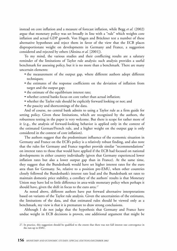
instead on core inflation and a measure of forecast inflation, while Begg et al. (2002)argue that monetary policy was set broadly in line with a “rule” which weights coreinflation and actual GDP growth. Von Hagen and Brückner test a number of thesealternative hypotheses and reject them in favor of the view that the ECB places disproportionate weight on developments in Germany and France, a suggestion considered and rejected by others (Alesina et al. [2001]).

To my mind, the various studies and their conflicting results are a salutaryreminder of the limitations of Taylor rule analysis: such analysis provides a usefulbenchmark for assessing policy, but it is no more than a benchmark. There are manyuncertain elements:

• the measurement of the output gap, where different authors adopt differenttechniques;

• the estimates of the response coefficients on the deviation of inflation from target and the output gap;

• the estimate of the equilibrium interest rate;• whether central banks focus on core rather than actual inflation;• whether the Taylor rule should be explicitly forward looking or not; and• the paucity and shortcomings of the data.And of course, no central bank admits to using a Taylor rule as a firm guide for

setting policy. Given these limitations, which are recognized by the authors, therobustness testing in the paper is very welcome. But there is scope for rather more ofit (e.g., the analysis of forward-looking behavior is applied only in the context of the estimated German/French rule, and a higher weight on the output gap is onlyconsidered in the context of core inflation).

The authors suggest that the predominant influence of the economic situation inGermany and France on the ECB’s policy is a relatively robust finding, and also notethat the rules for Germany and France together provide similar “recommendations”on interest rates to those that would have applied if the ECB had focused on nationaldevelopments in either country individually (given that Germany experienced lowerinflation rates but also a lower output gap than in France). At the same time, they suggest that the Bundesbank would have set higher interest rates for the euroarea than for Germany. So, relative to a position pre-EMU, when other countriesclosely followed the Bundesbank’s interest rate lead and the Bundesbank set rates tomaintain domestic price stability, a corollary of the authors’ results is that MonetaryUnion may have led to little difference in area-wide monetary policy when perhaps itshould have, given the shift in focus to the euro area.27

As noted above, different authors have put forward alternative interpretationsbased on variants of the Taylor rule analysis. Given the uncertainties of the estimates,the limitations of the data, and that estimated rules should be viewed only as abenchmark, my view is that it is premature to draw strong conclusions.

Although I do not judge that the hypothesis that Germany and France haveundue weight in ECB decisions is proven, one additional argument that might be


27. In practice, this suggestion should be qualified to the extent that there was not full interest rate convergence inthe run-up to EMU.

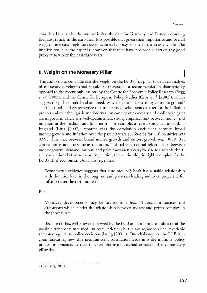
considered further by the authors is that the data for Germany and France are amongthe most timely in the euro area. It is possible that given their importance and overallweight, these data might be viewed as an early proxy for the euro area as a whole. Theimplicit result in the paper is, however, that they have not been a particularly goodproxy ex post over the past three years.

II. Weight on the Monetary Pillar

The authors also conclude that the weight on the ECB’s first pillar (a detailed analysisof monetary developments) should be increased—a recommendation diametricallyopposed to the recent publications by the Centre for Economic Policy Research (Begget al. [2002]) and the Centre for European Policy Studies (Gros et al. [2002]), whichsuggest the pillar should be abandoned. Why is this, and is there any common ground?

All central bankers recognize that monetary developments matter for the inflationprocess and that the signals and information content of monetary and credit aggregatesare important. There is a well-documented, strong empirical link between money andinflation in the medium and long term—for example, a recent study at the Bank ofEngland (King [2002]) reported that the correlation coefficient between broad money growth and inflation over the past 30 years (1968–98) for 116 countries was0.99, while that between broad money growth and output growth was –0.08. But correlation is not the same as causation, and stable structural relationships betweenmoney growth, demand, output, and price movements can give rise to unstable short-run correlations between them. In practice, the relationship is highly complex. As theECB’s chief economist, Otmar Issing, notes:

Econometric evidence suggests that euro area M3 both has a stable relationshipwith the price level in the long run and possesses leading indicator properties forinflation over the medium term.

But

Monetary developments may be subject to a host of special influences and distortions which render the relationship between money and prices complex inthe short run.28

Because of this, M3 growth is viewed by the ECB as an important indicator of thepossible trend of future medium-term inflation, but is not regarded as an invariableshort-term guide to policy decisions (Issing [2001]). One challenge for the ECB is incommunicating how this medium-term orientation feeds into the monthly policyprocess in practice, as that is where the main external criticism of the monetary pillar lies.

157

Comment

28. See Issing (2001).

The approach taken in the paper of estimating a P * or “money/price gap” modelappears to conform to the ECB’s broad framework quite well—a medium- or long-run divergence between the price level and its estimated (monetary) equilibrium provides explanatory power in an inflation equation. Again, though, there are dataand econometric challenges—the authors take issue with ECB on the measurementof money (in particular on the treatment of nonresident deposits) and also note thatwhile the euro-area money demand function appears relatively stable to date they do not identify a trend in velocity (in contrast to the ECB’s assessment). They alsoestimate a P * model without the long-run trend adopted by previous authors such asGerlach and Svensson (2001), on the reasonable premise that they wish to explaintrend inflation. But this approach may give rise to an econometric problem if there isan omitted trend that should be present in the equation, as the omission will affectthe estimated coefficients on the other variables.

The authors put forward two conclusions based on the P * analysis:• Excess money growth in 1999 contributed to higher inflation.• The inflationary spike of early 2001 was due to special factors.It would be helpful to provide additional information on the robustness of these

conclusions. Given the form of the preferred equation, it appears, by eye at least, fromFigure 5 (p. 137) that the lagged impact of the pickup in actual inflation during 1999and early 2000 might account for a considerable proportion of the rise in the consumerprice index (CPI) inflation forecast, with the price gap term making a relatively small contribution. To allay this concern, some statistics on the contributions of the pricegap term and the other terms to the within-sample fit over the past three years wouldbe useful. Is the price gap term providing much of the explanatory power in practiceover this period?

A major practical challenge with the authors’ recommendation is that it demandsa lot of the ECB in terms of being able to identify and interpret shocks in real time.At the start of Monetary Union in 1999, how easy was it to separate a genuine monetary shock from the possibility of a shock from the change in policy regime?And how easy was it to quantify the importance of special factors affecting inflationin 2001? The authors are attaching high weight to relatively simple money demandmodels. There are risks of over-reliance on such an approach, which may help toexplain the puzzle of why the study of the information content of money has faredrelatively poorly against a backdrop of a strong consensus that inflation is a monetaryphenomenon. More broadly, there are risks of asking too much of money demandmodels and condemning them when they fail to deliver, or—as in the currentpaper—having them deliver, but not in a fully convincing way.

I would be cautious in concluding from the evidence presented that more weightshould be added to the monetary pillar. I would nonetheless share much commonground with the authors. A broad conclusion among most central bankers is that estimates of long-run money demand and corresponding estimates of the excess stockof money are useful information variables. In turn, they pose important questionsand challenges on the sources of economic and financial shocks, which may providevaluable input to policy. But rarely can they act as a simple guide. I prefer to interpretthe authors’ results in that spirit.


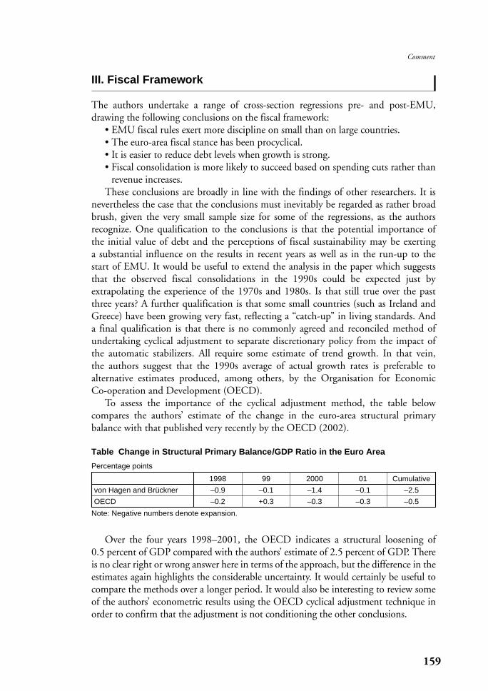
III. Fiscal Framework

The authors undertake a range of cross-section regressions pre- and post-EMU, drawing the following conclusions on the fiscal framework:

• EMU fiscal rules exert more discipline on small than on large countries.• The euro-area fiscal stance has been procyclical.• It is easier to reduce debt levels when growth is strong.• Fiscal consolidation is more likely to succeed based on spending cuts rather than

revenue increases.These conclusions are broadly in line with the findings of other researchers. It is

nevertheless the case that the conclusions must inevitably be regarded as rather broadbrush, given the very small sample size for some of the regressions, as the authors recognize. One qualification to the conclusions is that the potential importance ofthe initial value of debt and the perceptions of fiscal sustainability may be exerting a substantial influence on the results in recent years as well as in the run-up to thestart of EMU. It would be useful to extend the analysis in the paper which suggeststhat the observed fiscal consolidations in the 1990s could be expected just by extrapolating the experience of the 1970s and 1980s. Is that still true over the pastthree years? A further qualification is that some small countries (such as Ireland andGreece) have been growing very fast, reflecting a “catch-up” in living standards. Anda final qualification is that there is no commonly agreed and reconciled method ofundertaking cyclical adjustment to separate discretionary policy from the impact ofthe automatic stabilizers. All require some estimate of trend growth. In that vein, the authors suggest that the 1990s average of actual growth rates is preferable to alternative estimates produced, among others, by the Organisation for Economic Co-operation and Development (OECD).

To assess the importance of the cyclical adjustment method, the table below compares the authors’ estimate of the change in the euro-area structural primary balance with that published very recently by the OECD (2002).

159

Comment

Table Change in Structural Primary Balance/GDP Ratio in the Euro Area

Percentage points

1998 99 2000 01 Cumulative

von Hagen and Brückner –0.9 –0.1 –1.4 –0.1 –2.5

OECD –0.2 +0.3 –0.3 –0.3 –0.5

Note: Negative numbers denote expansion.

Over the four years 1998–2001, the OECD indicates a structural loosening of 0.5 percent of GDP compared with the authors’ estimate of 2.5 percent of GDP. Thereis no clear right or wrong answer here in terms of the approach, but the difference in theestimates again highlights the considerable uncertainty. It would certainly be useful tocompare the methods over a longer period. It would also be interesting to review someof the authors’ econometric results using the OECD cyclical adjustment technique inorder to confirm that the adjustment is not conditioning the other conclusions.

Von Hagen and Brückner end their paper by noting that “consolidation fatigue” issetting in and that winning support for further fiscal consolidation in a low-growthenvironment is proving difficult. As they note, the real challenge is to raise under-lying productivity growth in Europe through further structural reforms. The authorsargue that the fiscal rules are getting in the way—for example, by eliminating thescope to pursue reform programs that necessitate higher initial deficits, albeit withlower medium-term ones. More work in this area would be very welcome, as somereforms, for example, to increase work incentives by changes in benefit systems,would not appear to run foul of this critique.

To conclude, I think the paper is very interesting and raises much food forthought and further analysis. Any analysis of European Economic and MonetaryUnion is inevitably hampered by the lack of data to date. Many conclusions remainopen. The authors should be commended for attempting a rigorous study that setsout a useful route for further work as time progresses.


Alesina, Alberto, Olivier Blanchard, Jordi Galì, Francesco Giavazzi, and Harald Uhlig, “Defining aMacroeconomic Framework for the Euro Area,” Monitoring the European Central Bank, 3,Centre for Economic Policy Research, 2001.

Begg, David, Fabio Canova, Paul de Grauwe, Antonio Fatas, and Philip R. Lane, “Surviving theSlowdown,” Monitoring the European Central Bank, 4, Centre for Economic Policy Research,2002.

Faust, John, John H. Rogers, and Jonathan H. Wright, “An Empirical Comparison of Bundesbank andECB Monetary Policy Rules,” International Finance Discussion Paper No. 705, Board ofGovernors of the Federal Reserve System, 2001.

Gerlach, Stefan, and Lars E. O. Svensson, “Money and Inflation in the Euro Area: A Case for MonetaryIndicators,” Working Paper No. 98, Bank for International Settlements, 2001.

Gros, Daniel, Klaus Durrer, Juan Jimeno, Carlo Monticelli, and Roberto Perotti, “Fiscal and MonetaryPolicy for a Low-Speed Europe,” Fourth Annual Report of the CEPS Macroeconomic PolicyGroup, Centre for European Policy Studies, 2002.

Issing, Otmar, “The Importance of Monetary Analysis,” in Hans-Joachim Klöckers and CarolineWilleke, eds. “Monetary Analysis: Tools and Applications,” European Central Bank, 2001, pp. 5–7.

King, Mervyn, “No Money, No Inflation—The Role of Money in the Economy,” Bank of EnglandQuarterly Bulletin , 42 (2), 2002, pp. 162–177.

Organisation for Economic Co-operation and Development, OECD Economic Outlook, 71, 2002.Peersman, Gert, and Frank Smets, “The Taylor Rule: A Useful Monetary Benchmark for the Euro

Area,” International Finance, 2 (1), 1999, pp. 85–116.

References

Comment

STEFAN SCHÖNBERG

Deutsche Bundesbank

Most of Jürgen von Hagen and Matthias Brückner’s findings are plausible anddeserve support. This goes, in particular, for their conclusion that the experience

regarding monetary policy since the start of the European Monetary Union (EMU)has been more encouraging than with regard to fiscal policies. However, also in thearea of monetary policy, the first three and a half years of EMU give rise to a number of concerns:

(1) Due to the well-known time lags in the transmission process of monetary policy, the observed relatively low inflation rates in the euro area prevailingduring the first 12 to 18 months after entry into EMU have to be attributedlargely to the previous policy regime of the Bundesbank, which was de facto incharge of European monetary policy until the start of EMU. This means thatsince the point in time at which price developments in the euro area can berelated to the policy measures taken by the European Central Bank (ECB), theactual inflation rate, measured in terms of the harmonized consumer priceindex (HCPI), has been persistently above 2 percent, the upper bound of theECB’s definition of price stability over the medium term. Also worrying hasbeen the gradual rise in core inflation, which may be indicative of underlyingpressures gaining momentum. Should the ECB continue to miss its self-imposed target, it could be faced with a credibility problem—irrespective ofthe fact that the actual inflation rate has been strongly influenced by a numberof external shocks, notably the rise in oil prices. If such a sequence of “temporary” factors lasts long enough, it could become entrenched in Europe’sunderlying inflation rate and give rise to an increase in inflation expectations.Until now, however, this has not been the case, as inflation expectationsimplied by the pricing of inflation-indexed bonds and the recent rise of theeuro against other major currencies appear to suggest.

(2) Part of the explanation why consumer price index (CPI) inflation has beenovershooting the ECB’s target range is the fact that economic developments inthe euro area have continued to show significant divergences. This applies, inparticular, to the growth performance of euro-area member countries and to different cyclical patterns. Some of the inflationary pressures in the euro areaappear to reflect the fact that slow-growing countries have been experiencing a relatively sticky inflation rate and, hence, have not generated sufficient disinflation to offset the rise in inflation in the fast-growing ones. Under theseconditions, it has been difficult for the ECB to push average CPI inflation inthe euro area below the upper limit of its target range. A number of ECBobservers have suggested, therefore, that the target is too ambitious and shouldbe revised upward to take account of these difficulties. In more general terms, itcan be said that asymmetries and divergences in inflation developments amongmember countries raise additional problems for the conduct of the commonmonetary policy. Such problems can best be addressed by structural reformsaiming at raising the growth potential of countries that are lagging behind.

(3) Another problem relates to the ECB’s “two-pillar” strategy. The first pillar isdefined as a “reference value” for the annual growth rate of the broad monetary aggregate, M3. Since entry into EMU, M3 has grown at a rateconsistently higher than the reference value set by the ECB, except for a shortperiod at the end of 2000/beginning of 2001. Given the medium-term link

161

Comment

between money growth and inflation in the euro area von Hagen and Brücknerare referring to, their conclusion that the stance of monetary policy was too easyin 1999 and 2000 and that the resurgence of inflation in the euro area since the start of EMU must be attributed at least in part to the high money growthrates tolerated by the ECB appears prima facie correct.The ECB argues that a number of temporary factors have distorted M3 developments. Even if one follows this argument, the longer the ECB leaves interest rates unchanged whileM3 growth exceeds its preset reference value, the more the ECB’s two-pillarstrategy will come under pressure, giving renewed stimulation to public discussion about the relative importance of the two pillars. While the two-pillarstrategy offers a high degree of flexibility, it also entails a considerable amountof ambiguity and, hence, communication difficulties.

My conclusions arising from these considerations are similar to those drawn by von Hagen and Brückner: the ECB should be less concerned about short-termcyclical prospects and about the degree of capacity utilization in the euro area. Giventhat long-run monetary relations continue to be stable as observed by the authors,the ECB should give adequate weight to monetary developments in its decision-making process.

Von Hagen and Brückner’s assessment that on the fiscal side the picture duringthe first years of EMU is more mixed deserves support. However, some of the arguments the authors put forward for substantiating this judgment need to be qualified. Moreover, other factors that also explain the less satisfactory experiencewith fiscal policies in EMU are not mentioned.

(1) The authors’ finding that small countries typically pay more attention to thestrictures of the Stability and Growth Pact (SGP) appears to have been confirmed by recent events. A cause for concern is, above all, the expendituredrift in the three largest euro-area economies. If other member countries followthis behavior, the SGP could be rapidly undermined, with corresponding consequences for the functioning of EMU. The obvious conclusion for areform of the budgetary procedures of the European Union (EU) is to shift theaxis of power in economic policymaking by strengthening the role of the EUCommission and reducing the role of the national governments. Unfortunately,driven by member states’ desire to “move from technocracy to democracy,” theactual development goes rather in the opposite direction. Also, the authors’accurate observation that the fiscal rules introduced by EMU did not preventmember states from relaxing fiscal discipline after the decision on EMU membership had been taken is less the result of inappropriate rules than theconsequence of inherent weaknesses in the institutional arrangements. In particular, the fact that “sinners sit in judgment of other sinners” has madeenforcement of the rules difficult.

(2) The authors’ assertion that fiscal policy has been procyclical in the first years ofEMU deserves some qualification. First, while automatic fiscal stabilizers canmake some contribution to smoothing cyclical fluctuations, only EU membercountries that had not already achieved a fiscal position in balance or in surpluswere prevented from letting the automatic stabilizers operate fully. This effect,


however, was exactly what the fathers of the SGP had in mind when designingthe pact: the objective of reaching as quickly as possible a balanced budget wasconsidered more important than preserving fiscal room of maneuver for countries still running sizeable deficits. Second, it is often assumed that a loosening of fiscal policy has expansionary effects on the economy, at least inthe short term. In practice and under the conditions prevailing in the EU, the influence of fiscal policy on macroeconomic activity is uncertain, state-dependent, and generally small, and should therefore not be overestimated.This applies especially to an active anti-cyclical strategy by means of a discretionary fiscal policy that has additional well-known drawbacks.

(3) Von Hagen and Brückner also argue that the current fiscal framework isincomplete, because it does not give EMU member states enough guidance for the choice of a successful fiscal strategy. However, it should be stressed that the fiscal framework of the Maastricht Treaty was designed not to provide a framework for an optimal fiscal strategy under all circumstances but rather to provide safeguards against fiscal excesses to protect the commonmonetary policy. Insofar as the current fiscal framework respects the principles of the Maastricht Treaty, it leaves fiscal policy in the competence of individual member states and leaves the rights of national parliamentslargely untouched.

In summing up, it should be stated that the fiscal rules created by EMU are notperfect but appropriate enough to allow for the proper functioning of EMU. Thetrue risks derive from the inhibitions of national governments to fully implement theagreed rules. Several European governments have been calling for a “reinterpretation”of the SGP, ranging from applying the rules of the pact only to the EU as a whole (as opposed to individual member countries) to using cyclically adjusted figuresinstead of nominal figures, and/or to excluding certain expenditure categories fromthe calculation of the fiscal deficits. In the most recent instance, some governmentshave even made their commitment to further fiscal consolidation subject to achievingcertain growth objectives. All these explicit and implicit calls for an “SGP Lite”amount to a weakening of the pact. This could undermine confidence and in the endalso the proper functioning of EMU.

163

General Discussion

General Discussion

Responding to the comments of the discussants, Jürgen von Hagen stated that uncertainty has been taken into account in applying the Taylor rule by using variousspecifications to check the robustness of empirical results. He also emphasized therole of money supply in providing a guideline for medium- to long-term prices. Onfiscal issues, von Hagen commented that his basic results would not be altered by the use of alternative data, and that he was not arguing for the implementation ofprocyclical fiscal policy during an economic downturn as would be required understrict fiscal discipline.

In the general discussion, Pierre van der Haegen argued that actual policy decisions were based on a wide range of relevant available information, including thatrelated to money supply variables, and that the Taylor rule, which does not assignmonetary aggregates any roles in policymaking, cannot be used as a benchmark toassess the past record of the European Central Bank (ECB). Angel Palerm raiseddoubts about the stability of the inflation-unemployment relationship in Europe andstressed that without a stable Phillips curve the Taylor rule may not provide an adequate basis for comparative evaluations of monetary policy before and after theintroduction of the euro. Palerm and Gabriele Galati pointed out that changes haveoccurred in the transmission channel of monetary policies as a result of the launch ofthe European Monetary Union (EMU). In light of these structural changes, theyurged caution in using the Taylor rule in comparative evaluations.

Palerm and Masahiro Kawai (Ministry of Finance, Japan) both pointed out thatthe impact of interest rates on aggregate demand and the degree of synchronizationof a region’s business cycles would differ according to the level of economic integra-tion, and cast doubt on the justification of comparative evaluations based on theTaylor rule and the different evaluation results. Von Hagen responded to these pointsas follows. While it is too early to judge the degree of synchronicity of the region’sbusiness cycles, if major lags do in fact exist in these business cycles among membercountries, then the results of the analysis should be on the mark because the analysisfocuses on the major countries in terms of policy management, such as Germany andFrance. In this context, Palerm raised the question of whether the ECB’s 2 percentinflation ceiling was too low in light of the incomplete integration of the goods markets and the continued inflation rate differentials among EMU countries.

Regarding the monetary policy of the ECB, van der Haegen welcomed some ofthe results offered by von Hagen because they emphasize the importance of moneysupply, a key component of the ECB’s “two-pillar” strategy. Roberto Rinaldi (Bancad’Italia) addressed the policy action taken in early 2001, which has been interpretedas a measure toward monetary tightening by von Hagen, and asked how this could beconsistent with the International Monetary Fund’s (IMF’s) interpretation that thisaction represented monetary easing. Von Hagen argued that, at least in terms ofmoney supply, the policy action of early 2001 represented monetary tightening.Citing Germany’s high real interest rates and the views of market participants,Rinaldi then questioned the assertion that the economic situation of Germany hadbeen emphasized in the ECB’s policy.

Regarding fiscal policy, van der Haegen agreed with von Hagen’s statement thatthe credibility of fiscal policy commitments had an important bearing on confidencein the EMU. Rinaldi also expressed his agreement with von Hagen’s analysis. On theother hand, Maurice Obstfeld argued that it was necessary to mention the empiricalliterature on the importance of the structure of fiscal revenues and expenditures. As arationale for procyclical fiscal policies, Obstfeld argued that in addition to politicalfactors, there were certain economic factors which arose from the mutual interactionof fiscal discipline. On the question of how to improve fiscal discipline, von Hagenargued that while the fiscal authorities of member countries should be given more


discretion, the European Commission should be given the right to comment on thefiscal status of member countries.

Han Ming Zhi asked what the implications of the experiences of European Union(EU) integration were for Asian countries, which were in a very different stage of economic development.

In closing the session, Chairperson Jorge A. Braga de Macedo mentioned the importance of structural reform in the EMU member countries and argued that theEuropean experience presented other regions with the following two lessons: (1) theEuropean experience shows that economic integration is time consuming, althoughthe Americas and Asia might not need 50 years to achieve it; and (2) it is important forthe institutions involved in economic policy management to engage in cooperationand coordination on the international and regional levels.

165

General Discussion


Documents

Monetary and Fiscal Policy in the European Monetary Union · Monetary and Fiscal Policy in the European Monetary Union Jürgen von Hagen and Matthias Brückner ... monetary and fiscal