Fiscal Policy and Educational Attainment in the United States

IZA DP No. 1040

Fiscal Policy and Educational Attainmentin the United States - A GenerationalAccounting Perspective

Xavier ChojnickiFrédéric Docquier

DI

SC

US

SI

ON

PA

PE

R S

ER

IE

S

Forschungsinstitutzur Zukunft der ArbeitInstitute for the Studyof Labor

March 2004

Fiscal Policy and Educational

Attainment in the United States – A Generational Accounting Perspective

Xavier Chojnicki MEDEE, University of Lille 1

Frédéric Docquier CADRE, University of Lille 2,

IWEPS and IZA Bonn

Discussion Paper No. 1040 March 2004

IZA

P.O. Box 7240 53072 Bonn

Germany

Phone: +49-228-3894-0 Fax: +49-228-3894-180

Email: [email protected]

Any opinions expressed here are those of the author(s) and not those of the institute. Research disseminated by IZA may include views on policy, but the institute itself takes no institutional policy positions. The Institute for the Study of Labor (IZA) in Bonn is a local and virtual international research center and a place of communication between science, politics and business. IZA is an independent nonprofit company supported by Deutsche Post World Net. The center is associated with the University of Bonn and offers a stimulating research environment through its research networks, research support, and visitors and doctoral programs. IZA engages in (i) original and internationally competitive research in all fields of labor economics, (ii) development of policy concepts, and (iii) dissemination of research results and concepts to the interested public. IZA Discussion Papers often represent preliminary work and are circulated to encourage discussion. Citation of such a paper should account for its provisional character. A revised version may be available on the IZA website (www.iza.org) or directly from the author.

mailto:[email protected]

http://www.iza.org/

IZA Discussion Paper No. 1040 March 2004

ABSTRACT

Fiscal Policy and Educational Attainment in the United States - A Generational Accounting Perspective∗

In this paper, we investigate the consequences of the rise in educational attainment on the US generational accounts. We build on the 1995 accounts of Gokhale et al. (1999) and disaggregate them per schooling level. We show that low skill newborns are characterized by a negative generational account (-15.4% of their lifetime labor income) whilst medium and high skill newborns have positive accounts (26.8 and 32.3% of their lifetime labor income). Compared to Gokhale et al., our baseline forecast is more optimistic. Nevertheless, the rise in educational attainment is not strong enough to restore the generational balance. The current fiscal policy generates a long run deficit. Balancing the budget requires increasing taxes (by about 1.2%) or reducing transfers (by about 2.7%). These results are robust to growth and discounting assumptions, to the treatment of education spending. They are sensitive to assumptions about the schooling level of future generations. JEL Classification: E62, H6, J24 Keywords: generational accounting, human capital, fiscal policy Corresponding author: Frédéric Docquier CADRE University of Lille 2 1 Place Déliot 50984 Lille France Email: [email protected]

∗ We thank the participants to the Conference of the European Economic and Financial Society (Bologna, May 2003) for helpful comments. Suggestions from Gilles Duranton, Joël Hellier, and Philip Oreopoulos were very appreciated. We are grateful to Alan Auerbach, Tim Miller and Philip Oreopoulos for transmitting their program and dataset. The usual disclaimers apply.

mailto:[email protected]

1 Introduction

Since the seminal works of Auerbach, Gokhale and Kotliko¤ (1991, 1994), and Kot-

liko¤ (1992), generational accounting has usually been perceived as a meaningful way

to evaluate the sustainability of …scal policy. It builds on an original treatment of

the government’s intertemporal budget constraint: at any date, the present value of

government purchases must be covered by the current net public wealth, the present

value of net taxes which will be paid by living generations over the rest of their life-

time and the present value of net taxes which will be paid by future generations over

their whole lifetime. The basic questions are: what burden must the government leave

on future generations to remain solvent? Is the resulting …scal treatment of future

generations’ members identical to that of the current newborns?

Economically, there is no reason for equalizing individual taxes and transfers.

Most …scal regimes involve high taxes for high income individuals and low taxes for

less productive workers. The same rationale can be applied to intergenerational re-

distribution. If one generation is economically more productive than another (for

example because its proportion of rich agents is higher), it seems justi…ed to make it

pay more taxes or receive less transfers. The generational accounting methodology

partially takes account of di¤erences in generational wealth by comparing generations

in terms of …scal pressure rather than on gross burden. Using balanced growth as-

sumptions, the classical methodology de…nes the generationally balanced policy as a

situation in which individual taxes and transfers increase at the same pace as labor

3

productivity. However, existing generational accounting exercises rely on very simple

assumptions about the changes in labor productivity and/or lifetime labor income

across generations. Usually, these changes are related to a path of exogenous growth

rates that have no explicit link with the skill composition of the generations. Hence,

existing studies do not take account of an important source of heterogeneity within

and between generations, i.e. the rise in educational attainment of successive cohorts.

The purpose of this paper is to revisit the US accounts of Gokhale, Page and

Sturrock (1999)1 by introducing skill heterogeneity in the generational accounting

technique.2 GPS demonstrate that the US …scal policy is unsustainable and gener-

ationally imbalanced. They evaluate the …scal pressure imposed on a generation by

its lifetime net tax rate, i.e. the ratio of the present value (at birth) of net taxes one

generation has to pay to the government over its lifetime on the present value of its

lifetime labor income. They show that the lifetime net tax rate of future generations

amounts to 49.2%, to be compared with 28.6% for the current newborns. Such a

framework with a single representative agent within each generation fails to capture

the evolution of skills. In this paper, we demonstrate that it is crucial to introduce

skill heterogeneity for three main reasons:

1Henceforth GPS.2It should be noted that heterogeneity has already been introduced in the generational accounting

framework. Most existing works distinguish males and females. This can be important for illustrativepurpose but has a smaller incidence on long-run evaluations since the sex composition of living andfuture cohorts is extremely stable over time. Other studies such as Auerbach and Oreopoulos (2000)on the US, Bonin and al. (1999) on Germany or Collado and al. (2001) on Spain distinguishbetween natives and immigrants so as to evaluate the …scal e¤ect of immigration policies. This isobviously pertinent in countries where migrants represent a large share of the population and/orwhere selective immigration policies are explicit.

4

² …rstly, it concerns the US population as a whole;

² secondly, the age-pro…le of taxes and transfers is highly dependent on educa-

tional attainment. We distinguish three large categories of education: less than

high school (<HS), high school (HS) and more than high school (>HS). Ac-

cording to our estimations, the average lifetime income of a low skill individual

amounts to $81,373 to be compared to $174,293 for a medium skill worker and

$311,540 for a high skill worker. On the contrary, the present value of public

bene…ts received by an agent over her whole lifetime amounts to $58,063 for the

low skilled, $30,974 for the medium skilled and $21,373 for the high skilled;

² …nally, the skill composition of the population drastically changes over time

and is likely to evolve in future years. In 1995, numbers taken from Lee and

Miller (1997) reveal that 64 percent of the population aged 80 had a diploma

lower than high school, against 24 percent for those graduated from high school

and 12 percent for those higher than high school. For the cohort aged 55, these

numbers were respectively 21 percent, 38 percent and 41 percent. For the cohort

aged 30 in 1995, we have 13 percent, 35 percent and 52 percent. Obviously,

skill heterogeneity is very strong among living generations. According to the

forecasts of Lee and Miller (1997), these proportions are likely to change in

the future, respectively converging towards 10.9 percent, 28.9 percent and 60.2

percent for future cohorts of adults with completed schooling. Such a forecast

can be seen as a medium variant, lying between the ”low projection” and the

5

”high projection” of Cheeseman Day and Bauman (2000).

The rise in education attainment can be explained by several factors (public edu-

cation expenditures, rise in the skill premium...). For the next decades, the increase

in human capital per worker seems rather ineluctable as new educated cohorts will

progressively replace older less educated ones. These changes are likely to generate

…scal gains for the government. We argue that education is a key parameter for evalu-

ating the long-run sustainability of the current policy. By disregarding such changes,

the generational accounting technique induces two biases:

² extrapolating the living generation’s accounts on the basis of the current net tax

pro…le and common growth assumptions for taxes and bene…ts, the technique

is likely to lead to an underestimation of the net payments by living cohorts.

It makes little sense to assume that average net taxes of the generation aged

20 in 1995 can be projected on the basis on average net taxes paid by the

current older generations. Taking account of speci…c pro…les per schooling level

and changes in the skill composition of living cohorts allows to determine more

accurate path of net taxes for future years. This improves the evaluation of the

total burden left on future generations;

² evaluating the lifetime net tax rate of future generations must account for the

real lifetime labor income of these cohorts. These amounts obviously depend

on general assumption about total factor productivity but also on assumptions

about the skill composition of future generations. By disregarding the skill

6

structure of future generations, the accounting technique is likely to underesti-

mate the lifetime labor income of these cohorts.

In the rest of this paper, we show that the rise in educational attainment strongly

modi…es the conclusion of GPS. To make comparisons relevant, our analysis is also

based on the 1995 …scal year and our adjustment calculations rely on the counter-

factual hypothesis that all changes begin in 1995. Generally speaking, our paper

provides a sensitivity analysis to GPS benchmark assumptions. Our conclusions are

more optimistic and raise numerous issues about educational policies and social mo-

bility (how to increase the incentives to educate? Would the cost of increasing the

average schooling level exceed the …scal gains?), about the political sustainability of

current taxes and transfers (if the government de…cit decreases, will there be a …scal

pressure to reduce taxes or to increase transfers) and about the structure of the labor

market (can these …scal gains resist to the increasing supply of skills?). Nevertheless,

the only purpose of our contribution is to compute the impact of educational changes

on the government budget constraint all other things being constant, i.e. taking

the economic environment as given. Consequently, our results must exclusively be

appreciated in terms of …scal sustainability.

Section 2 discusses data issues and the calibration of net tax pro…les per age

and education level. It is shown that educational attainment a¤ects both taxes and

bene…ts. However, di¤erences in tax pro…les are stronger. Generational accounts

per skill are then computed in section 3. As in GPS, our basic assumptions about

7

the growth rates of per capita taxes and bene…ts build on the o¢cial projections

of the Congressional Budget O¢ce (CBO).3 The term ”…scal policy” then re‡ects

both the current age pro…le of net taxes (per age and educational level) and o¢cial

growth rates for per capita amounts. Our results indicate that low skill newborns are

characterized by a negative generational account (-15.4 percent of their lifetime labor

income). Lifetime net tax rates for medium and high skill newborns are positive and

amount to 26.8 percent and 32.3 percent.

Taking account of the rise in educational attainment has a strong impact on the

results. Compared to GPS, it is shown that the total burden left on future generations

is reduced by about 30.7 percent in our baseline scenario. Consequently, our results

are more optimistic. Nevertheless, we show that the drastic rise in educational attain-

ment do not restore the …scal sustainability. Balancing the long-run de…cit requires

increasing taxes (by about 1.2 percent) or reducing transfers (by about 2.7 percent).

This contrasts with the study of GPS which reveals that restoring the generational

balance in 1995 requires cutting all transfers by 17.5 percent or increasing all taxes

by 8.2 percent. Section 4 provides a similar exercise by considering public education

expenditures as transfers rather than a part of government purchases. Similar results

are obtained but the government de…cit becomes slightly higher than in the baseline

scenario. Restoring the balance allows to increase taxes by 1.4 percent or to cut

transfers by 2.4 percent. A sensitivity analysis is presented in section 5. Section 6

3See CBO (1997a, 1997b).

8

concludes. An appendix provides our mathematical tools for generational accounting

with heterogenous skills and an alternative simulation closer to the CBO aggregate

projections. However, we show that the latter scenario is rather inconsistent with

the assumption about labor productivity growth. We conclude that changes in edu-

cational attainment is a key parameter for analyzing the sustainability of the …scal

policy.

2 Data issues

Estimating the age pro…les of taxes and bene…ts for a reference year is the building

block for any longitudinal calculation. In this paper, we use GPS estimates of the

contemporary pro…les for men and women in 1995. We aggregate men and women

pro…les using sex composition data per age. These pro…les concern six types of tax

(Labor Income taxes, FICA taxes, Excise taxes, Capital Income taxes, Seignorage

taxes and Property taxes), seven types of bene…t (OASDI, Medicare, Medicaid, Un-

employment Insurance, General Welfare, AFDC and Food Stamps) and three items of

government purchases (Education expenditures, Federal government purchases and

State government purchases). These pro…les are scaled so as to match aggregated

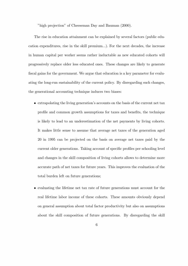
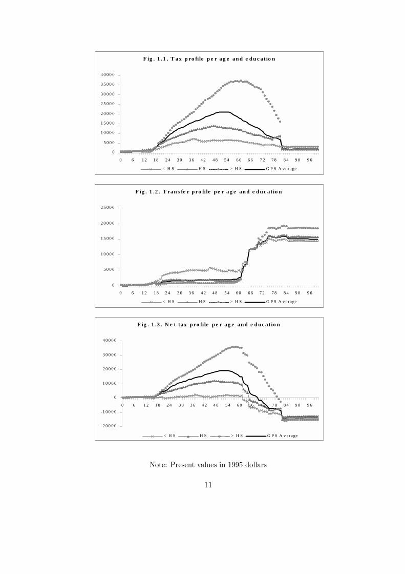
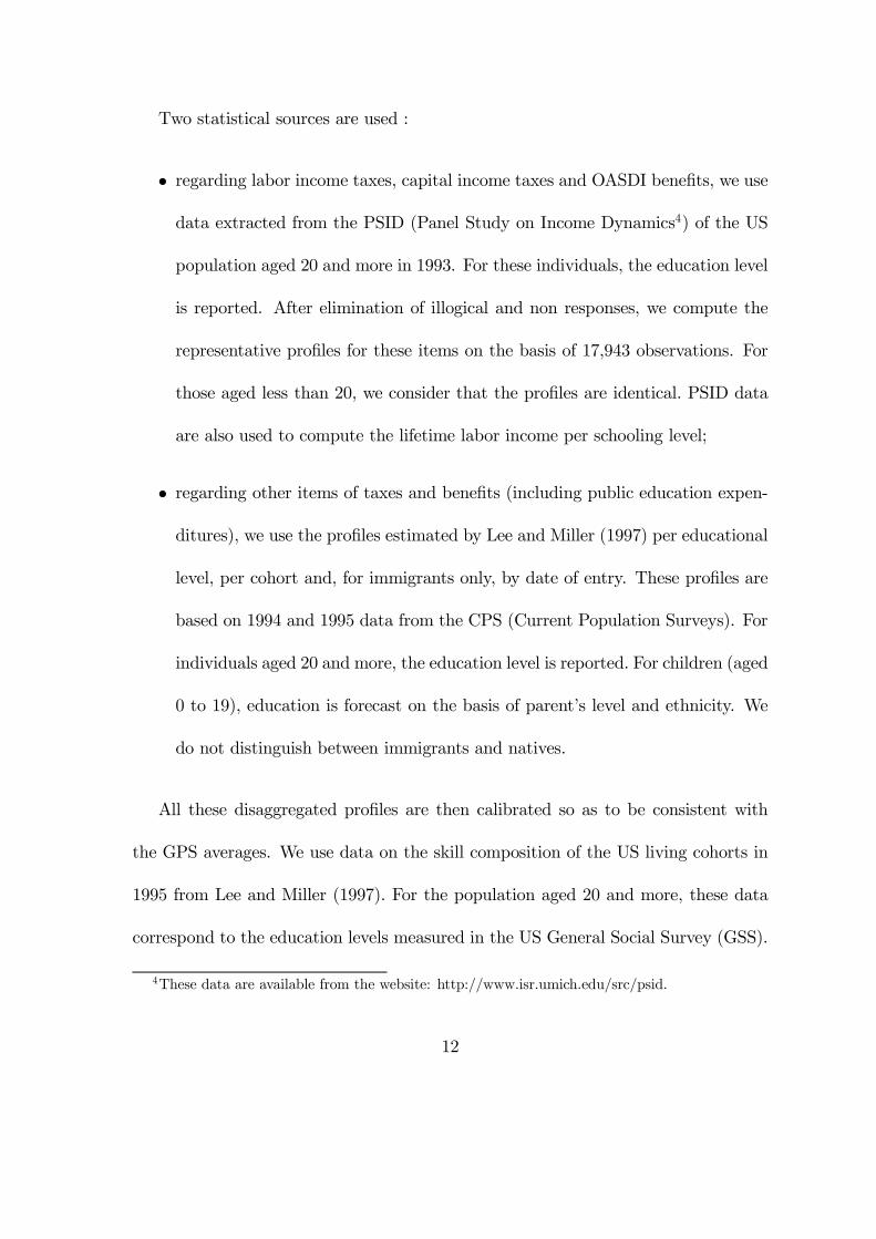
observations (i.e. the observed shares in GDP). The continuous lines (in black) on

…g. 1.1 and …g. 1.2 represent the total taxes and total bene…ts paid or received (ex-

cluding education spending) by the representative agent of each living cohort in 1995.

The continuous line (in black) on …g. 1.3 gives the di¤erence between taxes paid and

9

bene…ts received. It appears that net taxes are positive for individuals aged 15 to 70

(net contributors) and negative for individuals above age 70 (net bene…ciaries).

These representative pro…les represent the weighted average of net taxes paid

by all the US residents in 1995. These age-speci…c amounts are thus depending

on the average characteristics of living cohorts, i.e. on their sex composition, their

average skill levels, their nativity... In this paper, we disaggregate these amounts per

educational level. This requires disaggregating each tax or bene…t item of the GPS

dataset. Three educational levels are distinguished: individual with a less than high

school diploma (<HS), those with a high school diploma (HS) and those with a more

than high school diploma (>HS).

10

��

��

��

��

��

��

��

��

��

��

��

��

��

��

F ig . 1 .1 . T a x p ro file p e r a g e an d e d u c at io n

0

5 0 0 0

1 0 0 0 0

1 5 0 0 0

2 0 0 0 0

2 5 0 0 0

3 0 0 0 0

3 5 0 0 0

4 0 0 0 0

0 6 1 2 1 8 2 4 3 0 3 6 4 2 4 8 5 4 6 0 6 6 7 2 7 8 8 4 9 0 9 6

< H S H S��

> H S G P S A v erage

��

��

��

��

��

��

��

��

��

��

��

��

��

��

��

��

��

��

��

��

��

F ig . 1 .2 . T ran s fe r p ro file p e r ag e an d e d u c atio n

0

5 0 0 0

1 0 0 0 0

1 5 0 0 0

2 0 0 0 0

2 5 0 0 0

0 6 1 2 1 8 2 4 3 0 3 6 4 2 4 8 5 4 6 0 6 6 7 2 7 8 8 4 9 0 9 6

< H S H S��


��

��

��

��

��

��

��

��

��

��

��

��

F ig . 1 .3 . N e t tax p ro file p e r ag e an d e d u c a tio n

-2 0 0 0 0

-1 0 0 0 0

0

1 0 0 0 0

2 0 0 0 0

3 0 0 0 0

4 0 0 0 0

0 6 1 2 1 8 2 4 3 0 3 6 4 2 4 8 5 4 6 0 6 6 7 2 7 8 8 4 9 0 9 6

< H S H S��


Note: Present values in 1995 dollars

11

Two statistical sources are used :

² regarding labor income taxes, capital income taxes and OASDI bene…ts, we use

data extracted from the PSID (Panel Study on Income Dynamics4) of the US

population aged 20 and more in 1993. For these individuals, the education level

is reported. After elimination of illogical and non responses, we compute the

representative pro…les for these items on the basis of 17,943 observations. For

those aged less than 20, we consider that the pro…les are identical. PSID data

are also used to compute the lifetime labor income per schooling level;

² regarding other items of taxes and bene…ts (including public education expen-

ditures), we use the pro…les estimated by Lee and Miller (1997) per educational

level, per cohort and, for immigrants only, by date of entry. These pro…les are

based on 1994 and 1995 data from the CPS (Current Population Surveys). For

individuals aged 20 and more, the education level is reported. For children (aged

0 to 19), education is forecast on the basis of parent’s level and ethnicity. We

do not distinguish between immigrants and natives.

All these disaggregated pro…les are then calibrated so as to be consistent with

the GPS averages. We use data on the skill composition of the US living cohorts in

1995 from Lee and Miller (1997). For the population aged 20 and more, these data

correspond to the education levels measured in the US General Social Survey (GSS).

4These data are available from the website: http://www.isr.umich.edu/src/psid.

12

For the population aged 0 to 19 (those reaching age 20 between 1996 and 2015), Lee

and Miller (1997) forecast educational attainment on the basis of parents’ level of

education and ethnicity. Then, we consider that the skill structure of future cohorts

(aged 20 after 2015) is stationary. Compared to existing studies, our scenario can

be seen as a medium variant. It lies between the ”low projection” and the ”high

projection” provided in Cheeseman Day and Bauman (2000).

The …rst column of table 1 gives the cohort shares per educational level in 1995.

It appears that 52.0 percent of the population aged 30 has a diploma higher than high

school, against 35.0 percent for those graduated from high school and 13.0 percent

for those lower than high school. At 60 years old, these numbers were respectively

36.6 percent, 36.9 percent and 26.5 percent. For the newborns, they should be 60.2

percent, 28.9 percent and 10.9 percent.

The rest of table 1 thus provides age pro…les per educational level fully consistent

with the GPS estimates. We only report the main categories of taxes and transfers.

Fig. 1.1 to 1.3 give the disaggregation per schooling level of total taxes, total bene…ts

and net taxes for each living age group. The impact of educational attainment is

mainly perceptible for taxes: at 60 years old, the taxes paid by a high skill individual

are six times as large as the amount paid by a low skill individual. However, smaller

di¤erences are also appearing in bene…t pro…les. In terms of net taxes, low skill agents

are obviously the main bene…ciaries of the …scal policy whilst medium and high skill

agents are the contributors. At age 60, the ratio of net taxes between a high skilled

13

and a medium skilled is about 3.5. Hence, it makes no doubt that changes in the

educational structure strongly a¤ect the sustainability of the current …scal policy.

Table 1. Age profiles per educational level - 1995

Cohort Share

Labor Income Tax

Capital Income Tax FICA Tax

Other Taxes OASDI

Medicare & Medicaid

Other benefits

Less than High School0 10.9% 0 0 0 549 7 446 0

20 16.1% 336 -5 880 1545 13 669 145030 13.0% 1187 158 2086 1935 86 1863 246240 11.2% 1474 339 2185 2334 345 2406 225050 16.3% 1418 273 2288 2403 446 3109 143460 26.5% 995 490 1508 3172 1133 2995 86370 33.1% 153 692 211 3363 7320 5473 864100 64.0% 28 0 30 1472 7090 6787 450

High School0 28.9% 0 0 0 549 7 342 0

20 32.3% 1080 37 1365 2023 22 340 67530 35.0% 2655 262 3432 2749 67 786 108640 32.0% 3068 990 3761 4404 210 840 86050 35.2% 2963 1167 4036 5210 315 874 45760 36.9% 2015 1496 2472 5985 812 978 28270 36.5% 269 1851 301 6712 8870 5175 155100 24.0% 79 0 52 1918 8897 6666 140

More than High School0 60.2% 0 0 0 549 7 247 0

20 51.6% 1245 336 1332 2846 12 150 27230 52.0% 4439 1016 5001 5443 83 317 44440 56.8% 5356 2839 5955 9936 135 337 38550 48.6% 6019 4999 6184 15246 246 445 25760 36.6% 4211 7506 4434 20711 784 575 18070 30.4% 894 8690 952 22878 10012 5072 183100 12.0% 59 0 134 2973 11769 6593 116

Weighted average (a)0 - 0 0 0 549 7 296 0

20 - 1045 184 1270 2371 15 295 59130 - 3392 640 4073 4044 78 682 93140 - 4191 1969 4832 7318 183 729 74650 - 4196 2882 4795 9627 303 1029 51860 - 2549 3430 2935 10631 887 1365 39970 - 421 3547 469 10518 8704 5242 398100 - 44 0 48 1759 8085 6735 336

Note: (a) Weighted averages corresponding to GPS profilesSource: GPS; PSID; Lee and Miller (1997); Authors' calculations

14

3 Revisiting 1995 generational accounts

Let us now introduce the disaggregated net tax pro…les in the generational account-

ing framework. The starting point of generational accounting is the government’s

intertemporal budget constraint. At the base year 1995, the sum of the public net

wealth and the present value of prospective aggregate net payments by living and fu-

ture generations must equalize the present value of prospective public purchases. The

public net wealth is the only observable item of this constraint : it amounts to -$2.1

trillion in 1995. Regarding generational accounts of living and future generations, we

follow GPS and proceed as following.

Using assumptions about the time path of government purchases and individual

amounts of tax and transfer for living generations enables to derive the present value

of government purchases and payments by living generations. It is also possible to

compute the hypothetical generational accounts of future cohorts under the same

…scal policy than for living cohorts. Combining these amounts into the government

intertemporal budget constraint, we compute the …scal adjustment required to bal-

ance the budget. This adjustment a¤ects taxes and/or transfers from 1995 onwards.

Hence, it impacts on the situation of both living and future generations. Depending

on the type of adjustment we opt for, we compute the ”adjusted” generational ac-

counts of living and future generations that are budgetary sustainable. Finally, these

”adjusted” payments made by the newborns and individuals not yet born can be

compared on a lifetime basis. The technical appendix 8.1 describes our methodology.

15

The present value of government purchases (PVG). The PVG is the dis-

counted sum of government purchases (State and Federal purchases, including educa-

tional expenditures) from 1995 under the assumed …scal policy. Our baseline scenario

builds on GPS study. Through 2070, we then use the path of government purchases

simulated by the Congressional Budget O¢ce. Beyond 2070, government purchases

are supposed to grow by 1.2 percent per year. The baseline discount rate is 6 percent.

The present value of payments by living generations (PVL). The PVL

sums up generational accounts of all the members of living generations. By gener-

ational account, we mean the present value of net taxes that a member of a group

will pay over the rest of her life under the assumed …scal policy. Evaluating the ac-

counts of living generations then requires a long-run prospective calculations relying

on some crucial assumptions about the demographic size of each living generation, its

educational structure, the evolution of per capita taxes and bene…ts and the economic

environment. Here is a description of the main assumptions:

² our baseline scenario relies on the intermediate population projection of the

Social Security Administration (SSA), extended by GPS projections beyond

2070 (assuming that fertility, mortality and net immigration rates remain at

their 2070 level. This scenario implies a sharp deterioration of the old-age

dependency ratio (i.e. the ratio of people aged 65+ to people aged 15-64). The

ratio amounts to 19% in 2000 and is expected to reach more than 33% in 2050

and about 40% in 2100;

16

² the growth rates of per capita taxes and bene…ts are those used in GPS study,

themselves building on the reference projection of the Congressional Budget

O¢ce through 2070. A growth path is calculated for each item of tax and

bene…t. We equivalently apply these growth rates to per capita amounts paid

(or received) by the members of each educational category. For a given path of

growth rates, our …scal projections are a¤ected by the changes in educational

structure and in demographic size (while GPS/CBO aggregates are only a¤ected

by the demography). An alternative scenario would be to calibrate the growth

rates so as to match the CBO aggregate projections per item. Nevertheless,

appendix 8.2 shows that our baseline scenario is more consistent with the as-

sumption about labor productivity growth than aggregate budgetary forecasts5.

Consequently, our projections do not correspond to those of the Congressional

Budget O¢ce;

² the net tax pro…les are assumed to be stable over time. It could be argued that

the rise in educational attainment will impact on the return to skill and reduce

the gap between skilled and unskilled workers even if it did not happen in the

past decades (between 1970 and 2000, the return to skills has increased despite

a remarkable rise in educational attainment). It could also be argued that the

5The CBO projection does not take account of the rise in educational level of the population. Inappendix 8.2, we compare our baseline scenario (based on CBO growth rates for per capita taxesand transfers) with an alternative scenario based on CBO aggregated projections. This requirescalibrating the alternative growth rates of per capita taxes and bene…ts so as to match GPS/CBOaggregate amounts. Our calculations show that the resulting growth rates are hardly consistent withthe 1.2 percent growth rate of labor productivity.

17

rise in school attendance will change the average cost of education per student.

However, endogenizing the tax pro…les is beyond the scope of our accounting

study;

² the educational attainment of living generations in 1995 is depicted in table

1. For each living generation, the educational structure is assumed to be con-

stant over time. Given the absence of life table per educational attainment,

we disregard the e¤ect of heterogeneity in mortality (life expectancy is usually

higher for the high skilled) as well as the timing of immigration ‡ows (for young

generations, future immigration ‡ows are likely to reduce the share of skilled

workers over time);

² as for the PVG, the discount rate is set to 6 percent. The growth rate of indi-

vidual taxes and transfers beyond 2070 is set to 1.2 percent.

Generational accounts of living generations are given in table 2. It clearly appears

that the generational account of a low skill newborn is negative. On their whole

lifetime, unskilled agents are expected to receive more transfers than paying taxes to

the government. On the opposite, generational accounts of medium and high skill

individuals are positive. More particularly, the average generational account of a high

skill newborn is twice as large as the account of a medium skill newborn. It is also

worth noticing that generational accounts of low skill agents are always negative while

it is only the case after age 53 for the medium skilled and after age 64 for the high

skilled. To compare everyone on the same basis, GPS suggest to calculate the lifetime

18

net tax rates, i.e. the ratio of generational account on the present value of lifetime

labor income. This exercise can be done for each educational group. As it will appear

in table 3, the lifetime net tax rates of newborns amount to -15.4 percent for the low

skilled, 26.8 percent for the medium skilled and 32.3 percent for the high skilled. The

average lifetime net tax rate then amounts to 32.1% (against 28.6% in GPS study).

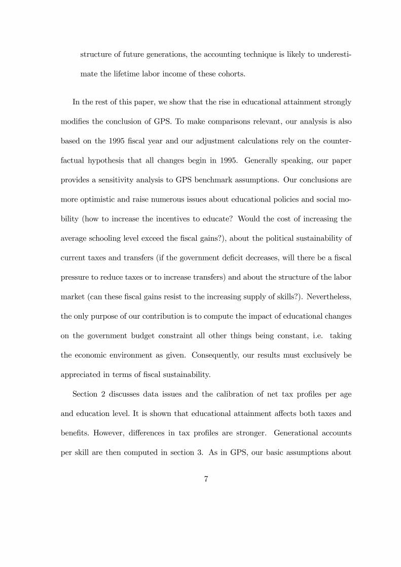
Given the changes in the skill composition of these living cohorts, our average

generational accounts per cohort are not identical to GPS amounts. This appears

on the bottom part of table 1 and on …g. 2. The di¤erences are small for old-age

cohorts rather large for young cohorts. Extrapolating the future taxes and transfers

of newborns on the sole basis of the contemporaneous pro…le, the classical method

underevaluates the newborns’ average account by 10.7 percent.

19

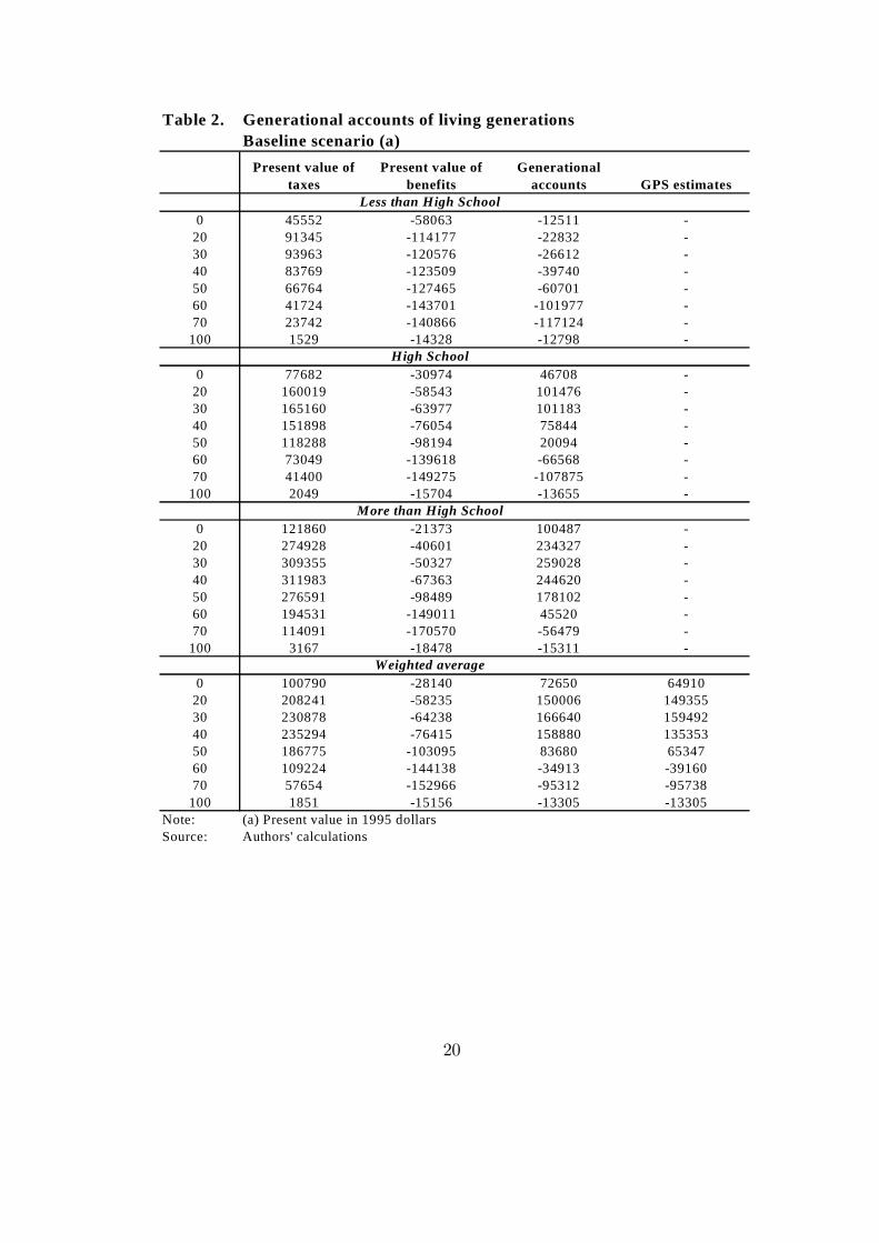
Table 2. Generational accounts of living generationsBaseline scenario (a)

Present value of taxes

Present value of benefits

Generational accounts GPS estimates

Less than High School0 45552 -58063 -12511 -

20 91345 -114177 -22832 - 30 93963 -120576 -26612 - 40 83769 -123509 -39740 - 50 66764 -127465 -60701 - 60 41724 -143701 -101977 - 70 23742 -140866 -117124 -

100 1529 -14328 -12798 - High School

0 77682 -30974 46708 - 20 160019 -58543 101476 - 30 165160 -63977 101183 - 40 151898 -76054 75844 - 50 118288 -98194 20094 - 60 73049 -139618 -66568 - 70 41400 -149275 -107875 -

100 2049 -15704 -13655 - More than High School

0 121860 -21373 100487 - 20 274928 -40601 234327 - 30 309355 -50327 259028 - 40 311983 -67363 244620 - 50 276591 -98489 178102 - 60 194531 -149011 45520 - 70 114091 -170570 -56479 -

100 3167 -18478 -15311 - Weighted average

0 100790 -28140 72650 6491020 208241 -58235 150006 14935530 230878 -64238 166640 15949240 235294 -76415 158880 13535350 186775 -103095 83680 6534760 109224 -144138 -34913 -3916070 57654 -152966 -95312 -95738

100 1851 -15156 -13305 -13305Note: (a) Present value in 1995 dollarsSource: Authors' calculations

20

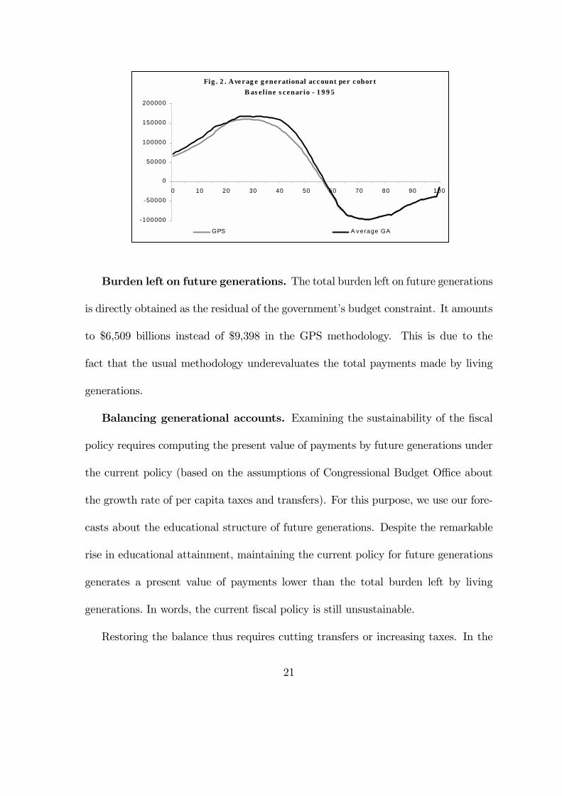
Fig . 2 . Ave rag e g ene rational acc ount per c ohor tB as e l ine s cenario - 1 9 9 5

-100000

-50000

0

50000

100000

150000

200000

0 10 20 30 40 50 60 70 80 90 100

GPS A v erage GA

Burden left on future generations. The total burden left on future generations

is directly obtained as the residual of the government’s budget constraint. It amounts

to $6,509 billions instead of $9,398 in the GPS methodology. This is due to the

fact that the usual methodology underevaluates the total payments made by living

generations.

Balancing generational accounts. Examining the sustainability of the …scal

policy requires computing the present value of payments by future generations under

the current policy (based on the assumptions of Congressional Budget O¢ce about

the growth rate of per capita taxes and transfers). For this purpose, we use our fore-

casts about the educational structure of future generations. Despite the remarkable

rise in educational attainment, maintaining the current policy for future generations

generates a present value of payments lower than the total burden left by living

generations. In words, the current …scal policy is still unsustainable.

Restoring the balance thus requires cutting transfers or increasing taxes. In the

21

classical method of generational accounting, such an adjustment is implemented by

multiplying net taxes of future generations by a constant adjustment factor. In our

case with heterogenous agents, such a rule would give rise to inconsistent results since

generational accounts are of opposite signs. For example, multiplying generational

accounts by 1.1 would induce more …scal e¤ort for individuals with a positive account

at birth, but a lower e¤ort for those with a negative account. Moreover, it seems quite

unrealistic to adjust the accounts of future generations only. As argued by Haveman

(1994), both living and future generations are likely to be concerned by …scal changes.

For these reasons, we use an adjustment method which concerns all the members of

all the generations. In a …rst step, we compute the present value of payments by

future generations under the current …scal policy. Comparing this amount to the

residual burden given by the budget constraint, we obtain the gap to be …nanced

by (in case of de…cit) or to be allocated to (in case of surplus) all living and future

generations. In a second step, we compute the proportional adjustment in all taxes

(or in all transfers) required to balance the budget. Finally, given the ”adjusted”

…scal policy, we derive the new generational accounts and lifetime net tax rate.6 Our

adjustment calculations rely on the counterfactual assumption that all changes begin

in 1995.

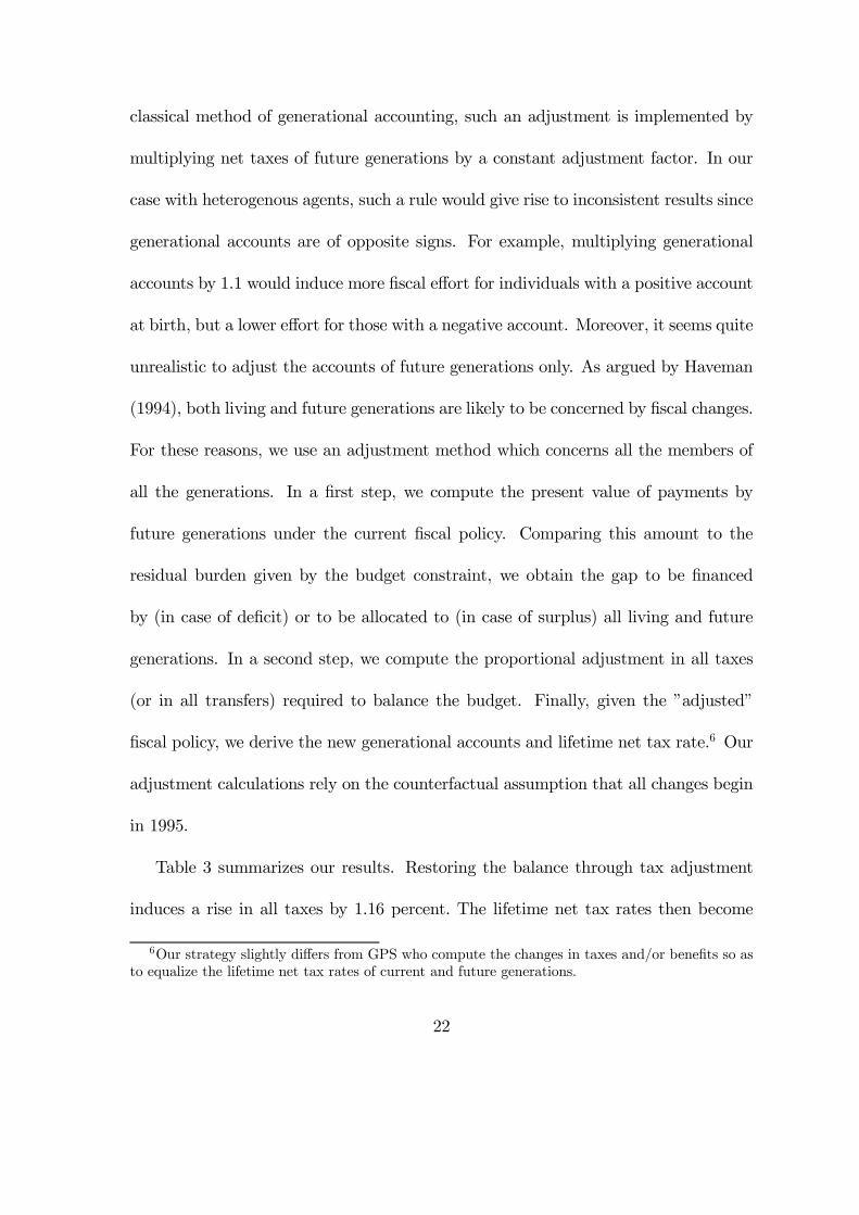
Table 3 summarizes our results. Restoring the balance through tax adjustment

induces a rise in all taxes by 1.16 percent. The lifetime net tax rates then become

6Our strategy slightly di¤ers from GPS who compute the changes in taxes and/or bene…ts so asto equalize the lifetime net tax rates of current and future generations.

22

-14.7 percent, 27.3 percent and 32.7 percent. Restoring the balance through transfer

adjustment induces a cut in all transfers by 2.68 percent. The lifetime net tax rates

then become -13.5 percent, 27.3 percent and 32.4 percent. These results contrast

with GPS who predict that generational balance requires increasing all taxes by 8.2

percent or reducing all bene…ts by 17.5 percent. This demonstrates the huge potential

impact of the rise in educational attainment in evaluating the long-run sustainability

of …scal policies.

Table 3. Generational imbalance and lifetime net tax ratesBaseline scenario (a)



Generational accounts

Lifetime Net Tax Rate (b)

Newborns' generational account and lifetime tax rate without policy adjustment<HS 45552 -58063 -12511 -15.4%HS 77682 -30974 46708 26.8%

>HS 121860 -21373 100487 32.3%Restoring the balance through tax adjustment (+1.16%)

<HS 46080 -58063 -11983 -14.7%HS 78582 -30974 47608 27.3%

>HS 123272 -21373 101899 32.7%Restoring the balance through transfer adjustment (-2.68%)

<HS 45552 -56504 -10952 -13.5%HS 77682 -30142 47540 27.3%

>HS 121860 -20800 101061 32.4%Note: (a) Present value in 1995 dollars

(b) Lifetime net tax rate = generational account / discounted lifetime labor incomeSource: Authors' calculations

23

4 Distributing education expenditures per age and

schooling level

In the line of GPS, let us now consider another scenario in which public education

expenditures (about one …fth of government purchases) are treated as individual

transfers. In our baseline scenario, education spending are evolving at the same pace

as the rest of government purchases such as defense or administration. In this new

scenario (labelled as ”Education Bene…t”), they evolve with the demography (the

number of individual in age of schooling), the educational composition of successive

cohorts (determining the length and the cost of schooling) and with common growth

assumption taken from GPS study. This scenario is then extremely important for our

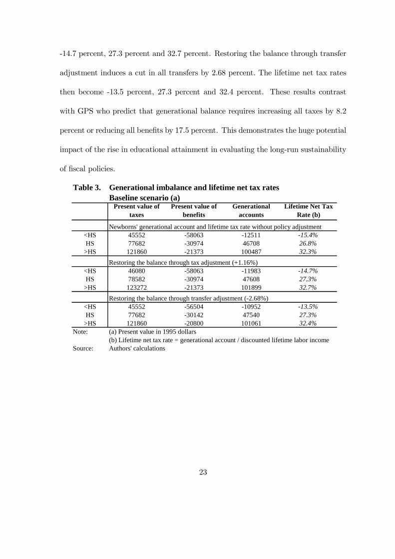
study. Table 4 gives the generational accounts of living generations.

24

Table 4. Generational accounts of living generationsEducation benefit scenario (a)



Generational accounts GPS estimates

Less than High School0 45552 -101081 -55529 -

20 91345 -117060 -25714 - 30 93963 -122286 -28322 - 40 83769 -124261 -40492 - 50 66764 -127653 -60888 - 60 41724 -143799 -102075 - 70 23742 -140893 -117151 -

100 1529 -14330 -12801 - High School

0 77682 -73246 4436 - 20 160019 -60986 99033 - 30 165160 -65687 99473 - 40 151898 -76805 75092 - 50 118288 -98381 19906 - 60 73049 -139715 -66666 - 70 41400 -149303 -107902 -

100 2049 -15707 -13658 - More than High School

0 121860 -80451 41409 - 20 274928 -56460 218468 - 30 309355 -52037 257318 - 40 311983 -68115 243868 - 50 276591 -98676 177915 - 60 194531 -149108 45423 - 70 114091 -170598 -56507 -

100 3167 -18480 -15313 - Weighted average

0 100790 -80613 20177 1315320 208241 -67668 140573 13986830 230878 -65948 164930 15778240 235294 -77166 158128 13460250 186775 -103282 83493 6515960 109224 -144235 -35011 -3925770 57654 -152993 -95339 -95765

100 1851 -15159 -13308 -13308Note: (a) Present value in 1995 dollarsSource: Authors' calculations

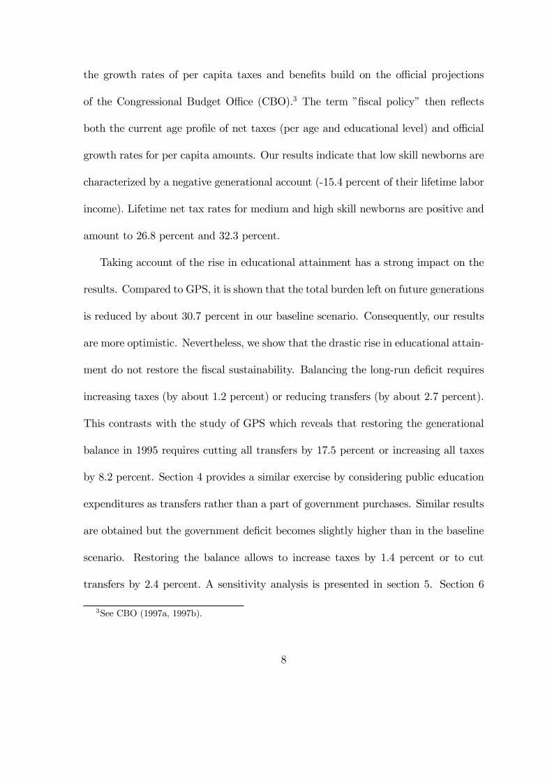
Treating education spending as bene…ts obviously reduces newborns’ accounts for

each schooling level. The di¤erences with the baseline scenario amounts to $43,000 for

the low skilled, $42,300 for the medium skilled and $59,000 for the high skilled. These

25

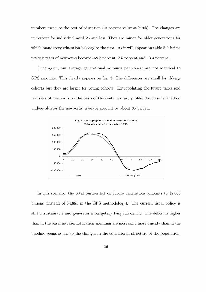
numbers measure the cost of education (in present value at birth). The changes are

important for individual aged 25 and less. They are minor for older generations for

which mandatory education belongs to the past. As it will appear on table 5, lifetime

net tax rates of newborns become -68.2 percent, 2.5 percent and 13.3 percent.

Once again, our average generational accounts per cohort are not identical to

GPS amounts. This clearly appears on …g. 3. The di¤erences are small for old-age

cohorts but they are larger for young cohorts. Extrapolating the future taxes and

transfers of newborns on the basis of the contemporary pro…le, the classical method

underevaluates the newborns’ average account by about 35 percent.

Fig . 3 . Averag e g enerational account per cohortEducation benefit s cenario - 1 9 9 5

-100000

-50000

0

50000

100000

150000

200000

0 10 20 30 40 50 60 70 80 90 100

GPS A v erage GA

In this scenario, the total burden left on future generations amounts to $2,063

billions (instead of $4,881 in the GPS methodology). The current …scal policy is

still unsustainable and generates a budgetary long run de…cit. The de…cit is higher

than in the baseline case. Education spending are increasing more quickly than in the

baseline scenario due to the changes in the educational structure of the population.

26

As depicted in table 5, restoring the balance through tax adjustment induces a rise in

all taxes by about 1.39 percent (against 5.0 percent in GPS framework). The lifetime

net tax rates then become -67.5 percent, 3.2 percent and 13.8 percent. Restoring

the balance through transfer adjustment induces a cut in all transfers by about 2.38

percent (against 13.0 percent in GPS framework). The lifetime net tax rates become

-65.3 percent, 3.5 percent and 13.9 percent.

Table 5. Generational imbalance and lifetime net tax ratesEducation benefit scenario (a)







<HS 46187 -101081 -54894 -67.5%HS 78766 -73246 5519 3.2%


<HS 45552 -98674 -53122 -65.3%HS 77682 -71502 6180 3.5%



5 Sensitivity analysis

Generational accounts depend on uncertain assumptions about demographic changes,

labor productivity growth rate, budgetary policy, interest rate and the future trends of

educational attainment. In this section, we analyze the sensitivity of our calculations

to alternative assumptions about growth and interest rates and about the educational

27

attainment of future cohorts.

As in GPS, our baseline scenario assumes a 6 percent discount rate and that

productivity increases by 1.2 percent a year. This discount rate is roughly equal to

the historical real rate of return on equity. A 1.2 percent productivity growth rate

is a reasonable value given the past trend of labor productivity. Table 6 reports

alternative projections when the interest rate amounts to 3 percent (a value closer

to the real return on government bonds) or 9 percent (a value closer to the return

on private capital) and when the labor productivity growth rate varies between 0.7

percent and 1.7 percent a year. These alternative scenarios are the same as those

used in GPS analysis. The results must be compared to the baseline scenario in

which education spending are included in government purchases.

Obviously, alternative assumptions about the rate of productivity growth have a

minor e¤ect on the results. Remember that the pure indexation of individual taxes

and bene…ts on productivity growth is implemented after the year 2070. Before that

date, the evolution of taxes and bene…ts relies on the CBO forecasts and is not

much a¤ected by the growth hypothesis. On the contrary, alternative assumptions

about the interest rate modify the calculations. The lifetime net tax rate of low skill

individuals is particularly a¤ected when the interest rate changes. However, interest

rates and growth rates do not modify the main result: in all cases, the current …scal

policy is unsustainable. The policy adjustments to restore the generational balance

are robust (especially when the interest rate increases). The tax variation ranges from

28

1.0 to 4.7 percent in the two extreme scenarios. Transfer cuts range from 2.5 to 9.0

percent.

Table 6. Generational accounts and budgetary adjustmentsSensitivity to discount and growth rate assumptionsNewborns' generational account and lifetime tax rate without policy adjustmentGenerational accounts Lifetime net tax rate

<HS g=0.007 g=0.012 g=0.017 g=0.007 g=0.012 g=0.017i=0.03 -88290 -89701 -91204 -34.4% -35.0% -35.5%i=0.06 -12391 -12511 -12638 -15.2% -15.4% -15.5%i=0.09 -1124 -1136 -1148 -3.8% -3.8% -3.9%

HS g=0.007 g=0.012 g=0.017 g=0.007 g=0.012 g=0.017i=0.03 88015 86535 84943 17.3% 17.0% 16.7%i=0.06 46840 46708 46565 26.9% 26.8% 26.7%i=0.09 22485 22470 22453 33.0% 33.0% 33.0%

>HS g=0.007 g=0.012 g=0.017 g=0.007 g=0.012 g=0.017i=0.03 278223 276415 274400 27.8% 27.7% 27.5%i=0.06 100677 100487 100270 32.3% 32.3% 32.2%i=0.09 40481 40453 40419 35.8% 35.8% 35.8%

Restoring the generational balance through…Tax change (in % of the current policy) Transfer change (in % of the current policy)

g=0.007 g=0.012 g=0.017 g=0.007 g=0.012 g=0.017i=0.03 3.5% 4.0% 4.7% -7.0% -7.8% -9.0%i=0.06 1.1% 1.2% 1.2% -2.5% -2.7% -2.9%i=0.09 1.0% 1.1% 1.1% -2.6% -2.7% -2.8%

Source: Authors' calculations

Finally, let us examine the sensitivity of our results to the assumptions about

educational attainment of young and future generations. Our baseline scenario is

based on Lee and Miller (1997). For the population aged 0 to 19 (those reaching age

20 between 1996 and 2015), Lee and Miller (1997) forecast educational attainment

on the basis of parents’ level of education and ethnicity. After 2015, we assume that

the skill structure of future cohorts (aged 20 after 2015) is stationary. Regarding

individuals who just completed schooling, the proportions of low, medium and high

skilled workers in 1995 are respectively 13, 35 and 52 percent. In 2005, Lee and

Miller forecast a slight decrease in educational attainment until 2005 (the proportions

become 16, 32 and 52 percent). Then the shares converge towards 10.9, 28.9 and 60.2

29

percent. These long-run proportion are reached in 2015. Compared to the study of

Cheeseman Day and Bauman (2000), the baseline scenario must be considered as a

reasonable medium variant.

Two alternative forecasts can be simulated. Building on the ”high projection”

of Cheeseman Day and Bauman (2000), the high variant is based on very optimistic

assumptions about future educational attainment. In the long-run, it assumes that

the proportions of high skilled workers aged 30 will reach 70.2 percent in 2030 (against

5.2 percent for low skilled workers and 24.6 for the medium skilled). Our ”low variant”

relies on the most pessimistic annual forecast from Lee and Miller. We keep the 2005

educational structure (16 percent for the low skilled, 32 and 52 percent for the medium

and high skilled) as constant after that year.

Table 7 gives the results. Clearly, newborns’ generational accounts and lifetime

net tax rates are quite stable. In terms of generational balance, the low variant

has a deep impact on the long run de…cit. Taxes must be increased by 5.69 percent

(instead of 1.16 in the baseline scenario) or transfers must be reduced by 12.52 per-

cent (instead of 2.68 in the baseline). Alternatively, the optimistic variant built on

Cheeseman Day and Bauman generates a long run budgetary surplus. A continued

rise in educational attainment would make the …scal policy sustainable: taxes could

be reduced by 1.3 percent or transfers could be increased by 3.13 percent. Of course,

reaching the high variant’s educational attainment would probably require a strong

expansionary education policy. If the marginal cost of education is increasing, the

30

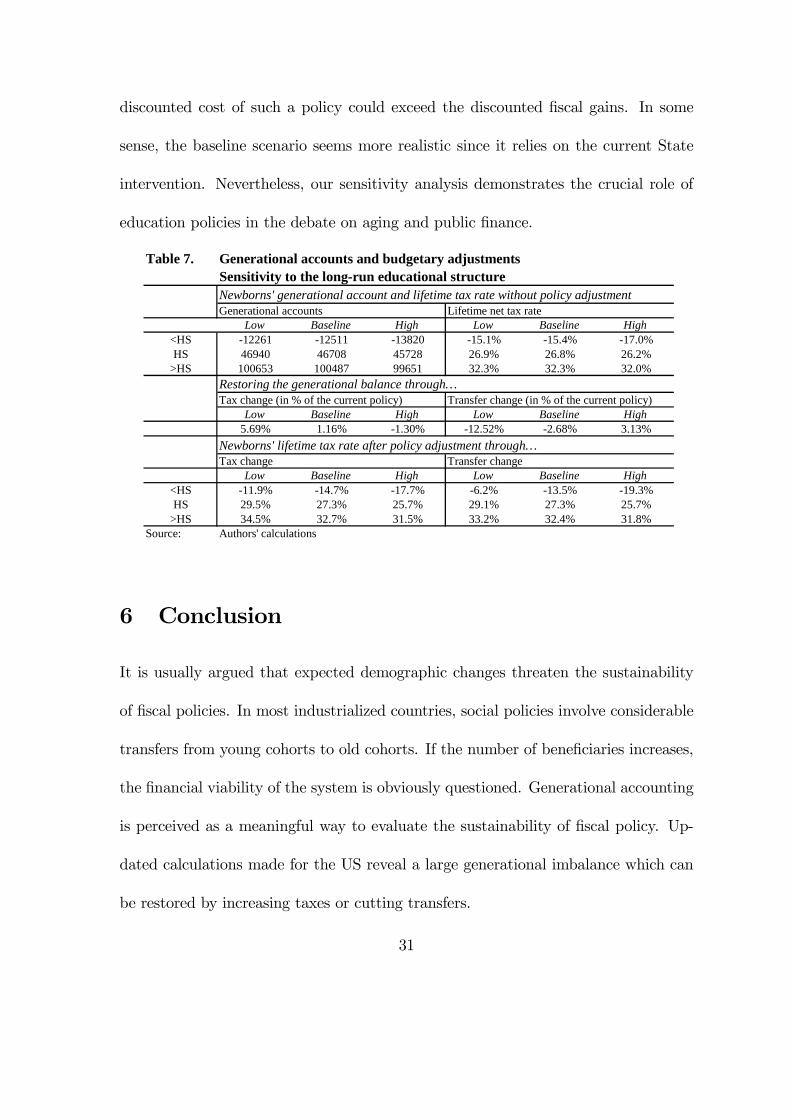
discounted cost of such a policy could exceed the discounted …scal gains. In some

sense, the baseline scenario seems more realistic since it relies on the current State

intervention. Nevertheless, our sensitivity analysis demonstrates the crucial role of

education policies in the debate on aging and public …nance.

Table 7. Generational accounts and budgetary adjustmentsSensitivity to the long-run educational structureNewborns' generational account and lifetime tax rate without policy adjustmentGenerational accounts Lifetime net tax rate

Low Baseline High Low Baseline High<HS -12261 -12511 -13820 -15.1% -15.4% -17.0%HS 46940 46708 45728 26.9% 26.8% 26.2%

>HS 100653 100487 99651 32.3% 32.3% 32.0%Restoring the generational balance through…Tax change (in % of the current policy) Transfer change (in % of the current policy)

Low Baseline High Low Baseline High5.69% 1.16% -1.30% -12.52% -2.68% 3.13%

Newborns' lifetime tax rate after policy adjustment through…Tax change Transfer change

Low Baseline High Low Baseline High<HS -11.9% -14.7% -17.7% -6.2% -13.5% -19.3%HS 29.5% 27.3% 25.7% 29.1% 27.3% 25.7%

>HS 34.5% 32.7% 31.5% 33.2% 32.4% 31.8%Source: Authors' calculations

6 Conclusion

It is usually argued that expected demographic changes threaten the sustainability

of …scal policies. In most industrialized countries, social policies involve considerable

transfers from young cohorts to old cohorts. If the number of bene…ciaries increases,

the …nancial viability of the system is obviously questioned. Generational accounting

is perceived as a meaningful way to evaluate the sustainability of …scal policy. Up-

dated calculations made for the US reveal a large generational imbalance which can

be restored by increasing taxes or cutting transfers.

31

To the best of our knowledge, these studies do not take account of a remarkable

change in the characteristics of people, the rise in educational attainment. This

change is budgetary important since it strongly modi…es the …scal means and needs of

successive generations. In this paper, we disaggregate tax and bene…t age-pro…les per

schooling level. This reveals strong di¤erences in net taxes among living generations.

Aggregating these net taxes on a whole lifetime basis, we show that the low skill

newborns’ account is negative (-15.4 percent of their lifetime labor income) whilst

medium and high skill newborns have positive accounts (26.8 percent and 32.3 percent

of their lifetime labor income). Taking account of the (past and expected) changes in

the educational structure avoids two sources of bias: the overestimation of the total

burden left on future generations and the underestimation of the …scal capacity of

these future generations.

Our results are more optimistic than those of existing studies. Our baseline sce-

nario indicates that the current …scal policy (de…ned by the current level of taxes

and transfers as well as by the growth assumptions of per capita taxes and bene-

…ts provided by the CBO) generates a long-run de…cit. However, the de…cit is much

lower than the GPS predictions. Restoring the generational balance requires cut-

ting transfers by 2.7 percent or increasing taxes taxes by 1.2 percent. These results

are quite robust to our assumptions about labor productivity growth, interest rate.

Treating education expenditures as transfers gives similar results. However, results

are sensitive to assumptions about the educational structure of future cohorts.

32

Is that a su¢cient reason to move from a highly pessimistic position to a highly

optimistic one? This strongly depends on the (at least relative) stability of net tax

pro…les per schooling level. We should keep in mind that generational accounting is a

pure mechanical projection tool which keeps these relative di¤erences as constant over

time. It does not take account of the interdependencies between the demography, the

changes in the educational structure and the economy. If young generations are more

and more educated, the average cost of education per student could be a¤ected. If

unskilled and skilled labor are imperfect substitutes on the labor market, an increase

in the supply of skills could give rise to a drop in the skill premium and a possible

rise in …scal needs of the highly skilled. We could then observe a shift of skilled

agents’ net taxes closer to unskilled agents’ ones. It is worth noticing that it did not

happen in the past. In spite of a huge rise in educational attainment, returns to skills

have also increased substantially over the last four decades. Moreover, recent theories

of endogenous technical biases suggest that a positive relationship between the skill

premium and the average level of schooling is likely to emerge in the long-run. As

argued by Acemoglu (2002), a rise in the education level of the labor force stimulates

investments in skill-consuming technical processes and increases the long run demand

for skilled workers. Compared to our predictions, this would reinforce the role of

education on public …nance. It is however di¢cult to forecast the evolution of the

skill premium without a long-run model of the US economy. Integrating generational

accounts and …scal policies in such a framework is obviously a promising issue that

33

we leave for further research.

7 References

² Acemoglu, D., 2002, ”Technical change, inequality and the labor market”, Jour-

nal of Economic Literature XL, 7-72.

² Auerbach, A.J., J. Gokhale and L.J. Kotliko¤, 1991, ”Generational accounts: a

meaningful alternative to de…cit accounting”, in Bradford, D. (ed.), Tax policy

and the economy, vol. 5, 55-110, Cambridge: MIT Press.

² Auerbach, A.J., J. Gokhale and L.J. Kotliko¤, 1994, ”Generational accounts:

a meaningful way to evaluate …scal policy”, Journal of Economic Perspectives

8(1), 73-94.

² Auerbach, A.J. and P. Oreopoulos, 1999, ”Analyzing the …scal impact of US

immigration”, American Economic Review 89, 176-180.

² Bonin, H., B. Ra¤elhüschen and J. Walliser, 2000, ”Can immigration alleviate

the demographic burden”, FinanzArchiv 57(1).

² Cheeseman Day, J. and K.J. Bauman, 2000, ”Have we reach the top? Ed-

ucational attainment projections of the US population”, Population Division

Working Paper, 43, US Census Bureau.

34

² Collado, M.D., I. Iturbe-Ormaetxe and G. Valera, 2001, ”Quantifying the im-

pact of immigration in the Spanish welfare state”, paper presented at the EEA

annual meeting, Lausanne.

² Congressional Budget O¢ce, 1997a, An economic model for long-run budget

simulations, CBO, July.

² Congressional Budget O¢ce, 1997b, The economic and budget outlook: an

update, US Government Printing O¢ce, September.

² Gokhale, J., B.R. Page and J.R. Sturrock, 1999, ”Generational accounts for

the United States: an update”, in Auerbach, A.J., L. J. Kotliko¤ and W.

Leibfritz (ed.), Generational Accounting Around the World, NBER Books, The

University of Chicago Press.

² Haveman, R., 1994, ”Should generational accounts replace public budgets and

de…cits?”, Journal of Economic Perspectives 8(1), 95-111.

² Kotliko¤, L.G., 1992, Generational accounting: knowing who pays, and when,

for what we spend, New York: The Free Press.

² Lee, R.D. and T. Miller, 1997, ”Immigrants and their descendants”, Project

on the economic demography of interage income reallocation, Demography, UC

Berkeley.

35

8 Appendix

8.1 Methodology with heterogenous agents

The starting point of the generational accounting technique is the government’s in-

tertemporal budget constraint. At the base year t, the sum of the public net wealth

and the present value of prospective aggregate net payments by living and future

generations must equalize the present value of prospective public purchases:

PV Lt + PV Ft +NWt = PV Gt (1)

where PV Lt measures the present value of net tax payments by living generations

over the rest of their life, PV Ft is the present value of net tax payments by future

generations, PV Gt stands for the present value of prospective government purchases

of goods and services and NWt is the net public wealth.

The net wealth at time t is observed. Two of the remaining terms are projected

using contemporaneous observations and o¢cial projections, PV Gt and PV Lt. The

fourth term, PV Ft, can thus be calculated as the residual burden bequeathed to

future generations.

The present value of government purchases is the discounted sum of public ex-

penditures:

PV Gt =1Xs=t

Gs(1 + i)s¡t

(2)

36

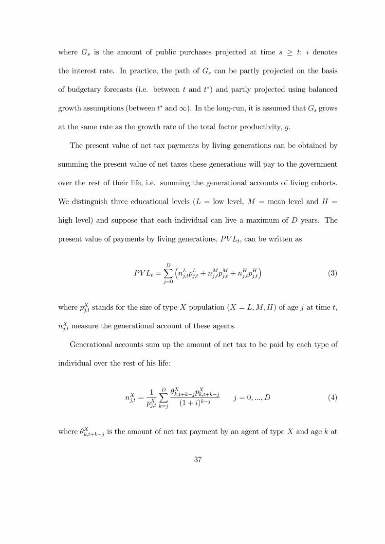
where Gs is the amount of public purchases projected at time s ¸ t; i denotes

the interest rate. In practice, the path of Gs can be partly projected on the basis

of budgetary forecasts (i.e. between t and t¤) and partly projected using balanced

growth assumptions (between t¤ and1). In the long-run, it is assumed that Gs grows

at the same rate as the growth rate of the total factor productivity, g.

The present value of net tax payments by living generations can be obtained by

summing the present value of net taxes these generations will pay to the government

over the rest of their life, i.e. summing the generational accounts of living cohorts.

We distinguish three educational levels (L = low level, M = mean level and H =

high level) and suppose that each individual can live a maximum of D years. The

present value of payments by living generations, PV Lt, can be written as

PV Lt =DXj=0

³nLj;tp

Lj;t + n

Mj;tp

Mj;t + n

Hj;tp

Hj;t

´(3)

where pXj;t stands for the size of type-X population (X = L;M;H) of age j at time t,

nXj;t measure the generational account of these agents.

Generational accounts sum up the amount of net tax to be paid by each type of

individual over the rest of his life:

nXj;t =1

pXj;t

DXk=j

µXk;t+k¡jpXk;t+k¡j

(1 + i)k¡jj = 0; :::; D (4)

where µXk;t+k¡j is the amount of net tax payment by an agent of type X and age k at

37

time t+ k ¡ j.

In practice, pXk;t+k¡j can be projected using demographic forecasts (including mor-

tality and net immigration ‡ows), data on schooling levels per age, and estimates for

the educational attainment of the young living generations after completion of their

education. The net taxes µXk;t+k¡j can be partly extrapolated on the basis of short-run

forecasts (taking account of o¢cial budgetary projections and potential …scal reforms

between t and t¤) and partly extrapolated using balanced growth assumptions (be-

tween t¤ and1). Typically, di¤erent assumptions can be considered for the items of

µXk;t+k¡j.

It should be noted that the generational accounts of the newborns, measuring the

present value of net taxes they expect to pay over their whole lifetime, need not to be

of the same sign. It can be negative for low skill individuals and positive for the high

skilled. These generational accounts can be expressed as percentage of the discounted

lifetime labor income, denoted by WX0;t for a newborn agent of type X. In the line of

GPS, this de…nes the lifetime net tax rate of the newborns:

LNRX0;t =nX0;tWX0;t

(5)

The basic issue of the generational accounting is the …nancial sustainability of

public policies. Given the generational account of the newborns at time t (nX0;t),

will it be possible to be so generous with future generations? The present value

of net tax payment by future generations, PV Ft, does not itself give an answer to

38

this question. To go further, one needs to transform this aggregate burden into an

individual amount, the average account of future cohorts.

One way to proceed is to compute the hypothetical generational accounts of future

cohorts under the current …scal policy. Using the same methodology than in (3) and

(4), we write:

PV F ¤t =1X

s=t+1

Min[s¡t¡1;D]Xj=0

µLj;spLj;s + µ

Mj;s+jp

Mj;s + µ

Hj;s+jp

Hj;s

(1 + i)s¡t(6)

where PV F ¤t measures the present value of net payments by future generations under

the assumption that the current …scal policy is sustainable.

This hypothetical value can then be compared to the residual value PV Ft com-

puted from (1):

² if PV F ¤t = PV Ft, the policy is sustainable and there is no need of …scal ad-

justment;

² if PV F ¤t > PV Ft, the government budget is in surplus so bene…ts could be

increased for the same levels of taxes;

² if PV F ¤t < PV Ft, the current policy is not sustainable or not generationally

balanced: it implies that either future generations must pay di¤erent net taxes

than current generations or current policy must be adjusted to restore sustain-

ability.

In case of unsustainability, the basic methodology suggest to adjust taxes and/or

39

transfers at some date. In this paper, we use an adjustment method which concerns

all the members of all the generations. If a gap has to be …nanced (in case of de…cit)

or allocated (in case of surplus), we compute the proportional adjustment in all taxes

(or in all transfers) required to balance the budget7.

Let us decompose the net taxes on all generations in two basic components, taxes

and bene…ts: µXj;s = µXT;j;s ¡ µXB;j;s. A time-invariant adjustment factor can be ap-

plied to each of these components (´T for taxes and ´B for bene…ts) so as to restore

sustainability. We then apply these proportional changes to both living generations

(over the rest of their lifetime) and future generations so as to balance the budget

constraint. Our adjustment rule is then summarized by the following set of equations:

PV Ladjt =DXj=0

DXk=j

XX=L;M;H

hµXT;k;t+k¡j(1 + ´T )¡ µXB;k;t+k¡j(1¡ ´B)

ipXk;t+k¡j

(1 + i)k¡j

PV F adjt =1X

s=t+1

Min[s¡t¡1;D]Xj=0

XX=L;M;H

hµXT;j;s(1 + ´T )¡ µXB;j;s(1¡ ´B)

ipXj;s

(1 + i)s¡t

PV Gt = PV Ladjt + PV F adjt +NWt

There is a continuum of pairs (´T ; ´B) restoring the balance. Two speci…c pairs

are usually considered, one with ´T = 0 if the balance is achieved through transfer

cuts and one with ´B = 0 if the balance is achieved through tax increases. For each

scenario, the lifetime tax rate of future generations can be computed and compared

to that of the current newborns.

7It should be noted that, in the line of GPS, the balance can also be restored through changesin government purchases

40

8.2 An alternative scenario: trusting CBO projections

The CBO projection does not take account of the rise in educational level of the pop-

ulation. Let us examine an alternative scenario where the growth rates of per capita

taxes and transfers are calibrated so as to match the CBO aggregated projections

(for each item). In that case, the average generational accounts of living generations

are almost identical to those reported in GPS study. Nevertheless, our methodology

allows to disaggregate living generations’ account by schooling level. In table A1, it

is shown that the lifetime net tax rate amounts to -26.0 percent for the low skilled,

22.7 percent for the medium skilled and 28.7 percent for the high skilled. Applying

CBO projections up to 2070 also determines the prospective contribution of future

generations. It is only after 2070 that the our calculations become highly sensitive

to the educational structure of the population. Our generational balanced policy is

thus very close to that suggested in GPS study. Restoring the balance requires in-

creasing all taxes by 8.16 percent or reducing all transfers by 17.54 percent (this is

not signi…cantly di¤erent from GPS).

Is this scenario based on CBO aggregated projections more consistent than our

baseline scenario? Our answer depends on the growth rates of per capita taxes and

bene…ts. Table A.2 compares the average growth rates per item for the period 2010-

2050. Our calculations indicate that the baseline growth rates are more consistent

with the 1.2 percent growth rate of labor productivity. This is especially the case for

individual taxes. In our baseline scenario, the growth rate of labor income tax, capital

41

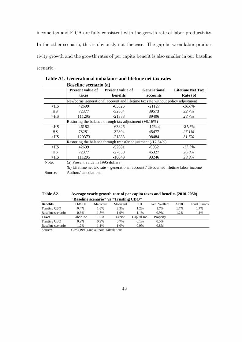
income tax and FICA are fully consistent with the growth rate of labor productivity.

In the other scenario, this is obviously not the case. The gap between labor produc-

tivity growth and the growth rates of per capita bene…t is also smaller in our baseline

scenario.

Table A1. Generational imbalance and lifetime net tax ratesBaseline scenario (a)







<HS 46182 -63826 -17644 -21.7%HS 78281 -32804 45477 26.1%


<HS 42699 -52631 -9932 -12.2%HS 72377 -27050 45327 26.0%



Table A2. Average yearly growth rate of per capita taxes and benefits (2010-2050)"Baseline scenario" vs "Trusting CBO"

Benefits OASDI Medicare Medicaid UI Gen. Welfare AFDC Food StampsTrusting CBO 0.4% 1.6% 2.3% 1.2% 1.7% 1.7% 1.7%Baseline scenario 0.6% 1.5% 1.9% 1.1% 0.9% 1.2% 1.1%Taxes Labor Inc. FICA Excise Capital Inc. PropertyTrusting CBO 0.9% 0.9% 0.7% 0.1% 0.5%Baseline scenario 1.2% 1.1% 1.0% 0.9% 0.8%Source: GPS (1999) and authors' calculations

42

Documents

Fiscal Policy and Educational Attainment in the United States