First Connectomics Challenge: From Imaging to Connectivityproceedings.mlr.press/v46/orlandi15.pdf · Orlandi Ray Battaglia Guyon Lemaire Saeed Statnikov Stetter Soriano methods, including

JMLR: Workshop and Conference Proceedings 46:1–22, 2015 ECML 2014

First Connectomics Challenge: From Imaging toConnectivity

Javier G. Orlandi∗ [email protected] i Constituents de la Materia, Univ. de Barcelona, Barcelona, Spain

Bisakha Ray∗ [email protected] for Health Informatics and BioinformaticsNew York University Langone Medical Center, New York, NY, USA

Demian Battaglia [email protected]. for Systems Neuroscience, Univ. Aix-Marseille, Marseille, FranceBernstein Ctr. for Computat. Neurosci., Gottingen, Germany

Isabelle Guyon [email protected], Berkeley, CA

Vincent Lemaire [email protected] Labs, Lannion, France

Mehreen Saeed [email protected]. Univ. of Computer Emerging Sci., Lahore, Pakistan

Alexander Statnikov [email protected] for Health Informatics and BioinformaticsNew York University Langone Medical Center, New York, NY, USA

Olav Stetter [email protected] Planck Inst. for Dynamics and Self-Organization, Gottingen, GermanyBernstein Ctr. for Computat. Neurosci., Gottingen, Germany

Jordi Soriano [email protected]

Estructura i Constituents de la Materia, Univ. de Barcelona, Barcelona, Spain

Editors: Demian Battaglia, Isabelle Guyon, Vincent Lemaire, Jordi Soriano

Abstract

We organized a Challenge to unravel the connectivity of simulated neuronal networks. Theprovided data was solely based on fluorescence time series of spontaneous activity in a net-work constituted by 1000 neurons. The task of the participants was to compute the effectiveconnectivity between neurons, with the goal to reconstruct as accurately as possible theground truth topology of the network. The procured dataset is similar to the one measuredin in vivo and in vitro recordings of calcium fluorescence imaging, and therefore the algo-rithms developed by the participants may largely contribute in the future to unravel majortopological features of living neuronal networks from just the analysis of recorded data,and without the need of slow, painstaking experimental connectivity labeling methods.Among 143 entrants, 16 teams participated in the final round of the challenge to competefor prizes. The winners significantly outperformed the baseline method provided by the or-ganizers. To measure influences between neurons the participants used an array of diverse

∗ The two first authors contributed equally.

c© 2015 J.G. Orlandi, B. Ray, D. Battaglia, I. Guyon, V. Lemaire, M. Saeed, A. Statnikov, O. Stetter & J. Soriano.

Orlandi Ray Battaglia Guyon Lemaire Saeed Statnikov Stetter Soriano

methods, including transfer entropy, regression algorithms, correlation, deep learning, andnetwork deconvolution. The development of “connectivity reconstruction” techniques isa major step in brain science, with many ramifications in the comprehension of neuronalcomputation, as well as the understanding of network dysfunctions in neuropathologies.

Keywords: neuronal networks, effective connectivity, fluorescence calcium imaging, re-construction, graph-theoretic measures, causality.

1. Introduction

All living neuronal tissues, from the smallest in vitro culture up to the entire brain, exhibitactivity patterns that shape the modus operandi of the network. Activity may take theform of spontaneous discharges, as occurs in the absence of stimuli, or in the form ofprecise patterns of activity during information processing, memory, or response to stimuli.A major paradigm in modern neuroscience is the relation between the observed neuronalactivity (function) and the underlying circuitry (structure). Indeed, activity in a livingneuronal network is shaped by an intricate interplay between the intrinsic dynamics of theneurons and their interconnectivity throughout the network.

In the quest for understanding the structure-function relationship, the neurosciencecommunity has launched a number of endeavors which, in an international and cooperativeeffort, aim at deciphering with unprecedented detail the structure of the brain’s circuitry(connectome) and its dynamics (Kandel et al., 2013; Yuste and Church, 2014). In Europe,the Human Brain project aspires at developing a large-scale computer simulation of thebrain, taking advantage of the plethora of data that is continuously being gathered. In theUnited States, the BRAIN Initiative aims at developing technologies to record neuronalactivity in large areas of the brain, ultimately linking single-cell dynamics, connectivity,and collective behavior to comprehend brain’s functionality. The difficulty and high costof these quests (Grillner, 2014) have called for parallel, more accessible strategies that cancomplement these large-scale projects.

With the hope to delineate parallel strategies in the understanding of neuronal circuits,we launched in April 2014 a ‘Connectomics Challenge’ aimed at developing computationaltools to answer a simple yet defying question: how accurately can one reconstruct theconnectivity of a neuronal network from activity data? To shape the challenge, we builta numerical simulation in which we first designed a neuronal circuit, therefore establishingits ground–truth topology, and later simulated its dynamics considering neurons as leakyintegrate-and-fire units. We also modeled the recording artifacts and noise associated withcalcium imaging.

The network that we simulated mimics the spontaneous activity observed in neuronalnetworks in vitro. Neuronal cultures, i.e. neurons extracted from brain tissue and grown ina controlled environment (Figure 1A), constitute one of the simplest yet powerful experi-mental platforms to explore the principles of neuronal dynamics, network connectivity, andthe emergence of collective behavior (Eckmann et al., 2007; Wheeler and Brewer, 2010).The relative small size of these networks, which typically contain a few thousand neurons,allows for the monitoring of a large number of neurons or the entire population (Spira andHai, 2013; Orlandi et al., 2013; Tibau et al., 2013). The subsequent data analysis —oftenin the context of theoretical models— provides the basis to understand the interrelationbetween the individual neuronal traces, neuronal connectivity, and the emergence of collec-

2

Connectomics Challenge

E+I

500 mm

Neuronal culture Detail FluoresenceA

100 mm

100 mm

1

2

3

10 s

Spontaneous activity traces

backgroundfluorescence

network burst500 mm

B

isolated firing events

Figure 1: Experimental motivation. (A) Example of a neuronal culture, derived from a ratembryonic cortex and containing on the order of 3000 neurons. The detail shows a small areaof the network in bright field and fluorescence, depicting individual neurons. In a typicalexperiment, neurons are identified as regions of interest (yellow boxes), and their analysisprovide the final fluorescence times series to be analyzed. (B) Fluorescence spontaneousactivity traces for 3 representative neurons. Data are characterized by a background signalinterrupted either by episodes of coherent activity termed network bursts, or by individualfiring events of relative low amplitude and occurrence.

tive behavior. Activity in cultures can be recorded by a number of techniques, from directelectrical measurements (Spira and Hai, 2013) to indirect measurement such as fluorescencecalcium imaging (Grienberger and Konnerth, 2012; Orlandi et al., 2013), which uses theinflux of Calcium upon firing to reveal neuronal activation (Figure 1B). Although Calciumimaging has a typical temporal resolution on the order of ms, its non-invasive nature andthe possibility to simultaneously access a large number of neurons with accurate spatialresolution (only limited by the optical system for measurements) have made it a very at-tractive experimental platform both in vitro and in vivo (Bonifazi et al., 2009; Grewe et al.,2010).

2. Challenge Design

The goal of the Challenge was to identify directed connections of a neuronal network fromobservational data. Using this kind of data constitutes a paradigm shift from traditionalapproaches based on interventional data and causal inference, where a planned experimentis required to perturb the network and record its responses. Although interventional ap-proaches are required to unambiguously unravel causal relationships, they are often costlyand many times technically impossible or unethical. On the other hand, observationaldata, which means recordings of an unperturbed system, can be used to study much largersystems and for longer periods.

The data for the challenge was generated using a simulator previously studied and vali-dated (Stetter et al., 2012; Orlandi et al., 2014) for neuronal cultures. As shown in Figure 1,mature neuronal cultures usually develop into a bursting regime, characterized by long peri-ods of very low neuronal activity and short periods of very high (bursting) activity (Orlandiet al., 2013; Tibau et al., 2013). This is a very interesting regime to check connectivity

3


A B

C

fluo

resc

en

ce (

a.u

.)

time(s)

ne

uro

n in

de

x

25 30 35 40 45

1

2

3

Figure 2: Simulated neuronal network for the Challenge. (A) The designed network con-tained 1000 neurons preferentially connected within 10 communities (marked with differentcolors in the figure), and with additional connections between communities. Each neuronconnected on average with 30 other neurons. (B) A detail of the connections of a single neu-ron. For clarity, only 50% of the connections are shown. (C) Top: Raster plot showing thespontaneous activity of 3 randomly chosen neurons in the network. Bottom: Correspondingfluorescence traces. Note the existence of both network bursts and isolated firings. Tracesare vertically shifted for clarity.

4


inference algorithms, since the system switches from a scenario where connections play al-most no role to another one where the system appears to be highly coherent with effectiveall-to-all connectivity profiles (Stetter et al., 2012). Although these two dynamic statesshape different effective connectivities, the actual structural connectivity layout remainsunchanged.

Connectivity inference techniques have usually focused on analyzing spiking data, withbinary signals identifying the presence (1) or absence (0) of neuronal firing. However,real spiking data are only available for a narrow set of experimental systems, and usuallyinvolve invasive electrode arrays or single-cell (path clamp) techniques. Recent advancesin imaging allow the simultaneous recording of thousands of neurons (Ohki et al., 2005;Panier et al., 2013). However, the identification of single spikes in imaging data cannotalways be accomplished and one has to directly analyze the fluorescence signals. Our dataalso take that into account and the signal given to participants models the fluorescencesignal of a calcium marker activated when a neuron fires. It also takes into account most ofthe experimental limitations, such as low acquisition speed, noisy data, and light scatteringartifacts (Stetter et al., 2012). The latter is important, since the fluorescence of a neuroninfluences the neighboring ones, giving rise to correlations between signals that are spurious.

The major features of the simulated networks for the Challenge are the following:

• Network structure. Our simulated data is inspired on experimental recordings inan area of roughly 1 mm2 (Stetter et al., 2012; Tibau et al., 2013). In that regionall neurons are able to physically reach any other neuron and the network can beconsidered as a random graph. For the small training datasets we used N = 100neurons with an average connectivity of 〈k〉 = 12 and varying levels of clustering1, from0.1 to 0.6, and the neurons were placed randomly in a 1× 1 mm square area (Guyonet al., 2014). For the larger datasets however, we used a different network structurethat was never revealed to the participants. This network is shown in Figure 2A,and its reconstruction by the participants shaped the overall goal of the challenge.Those datasets (including the ones used for the final scores) consisted of N = 1000neurons. The neurons were distributed in 10 subgroups of different sizes, and eachneuron connected with other neurons in the same subgroup with the same probability,yielding an internal average connectivity of 〈ki〉 = 10. Each subgroup had a differentinternal clustering coefficient, ranging from 0.1 to 0.6. Additionally, each neuron wasrandomly connected with 〈ko〉 = 2 other neurons of a different subgroup (Figure 2B).All the neurons were then randomly placed on a 1×1 mm square area and their indicesrandomized, so the network structure was not obvious in the adjacency matrix. Infact, none of the participants reported any knowledge of the real network topology.

• Neuron dynamics. We used leaky integrate and fire neurons with short term synap-tic depression, implemented in the NEST simulator (Gewaltig and Diesmann, 2007).For the small networks, N = 100, the synaptic weights were the same for any neuronand were obtained through an optimization mechanism to reproduce the observed ex-perimental dynamics with a bursting rate of 0.1 Hz. For the big networks, N = 1000,we ran the optimization mechanism independently for each subnetwork and then for

1. Understood as the “average clustering coefficient” in network theory, i.e. the number of triangles a neuronforms with its neighbors over the total number of triangles it could form given its connectivity.

5


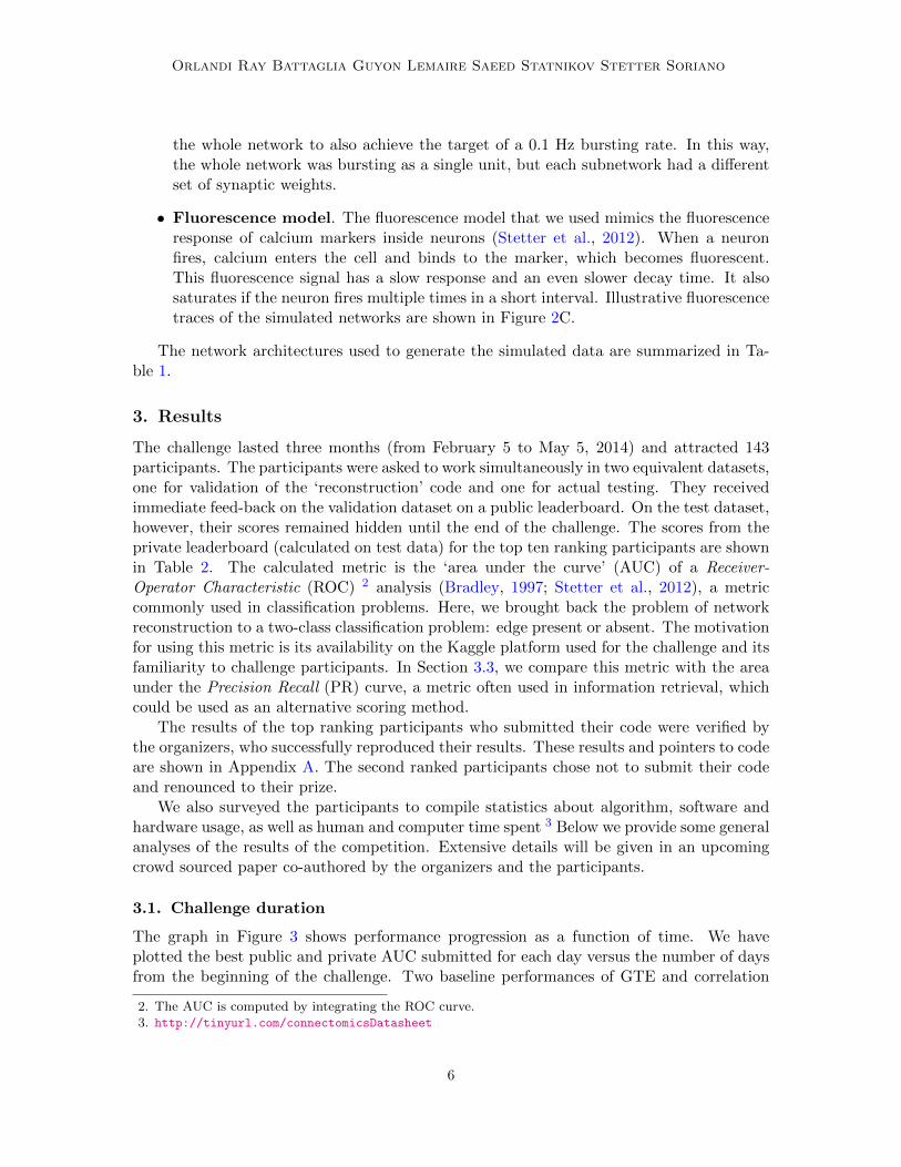
the whole network to also achieve the target of a 0.1 Hz bursting rate. In this way,the whole network was bursting as a single unit, but each subnetwork had a differentset of synaptic weights.

• Fluorescence model. The fluorescence model that we used mimics the fluorescenceresponse of calcium markers inside neurons (Stetter et al., 2012). When a neuronfires, calcium enters the cell and binds to the marker, which becomes fluorescent.This fluorescence signal has a slow response and an even slower decay time. It alsosaturates if the neuron fires multiple times in a short interval. Illustrative fluorescencetraces of the simulated networks are shown in Figure 2C.

The network architectures used to generate the simulated data are summarized in Ta-ble 1.

3. Results

The challenge lasted three months (from February 5 to May 5, 2014) and attracted 143participants. The participants were asked to work simultaneously in two equivalent datasets,one for validation of the ‘reconstruction’ code and one for actual testing. They receivedimmediate feed-back on the validation dataset on a public leaderboard. On the test dataset,however, their scores remained hidden until the end of the challenge. The scores from theprivate leaderboard (calculated on test data) for the top ten ranking participants are shownin Table 2. The calculated metric is the ‘area under the curve’ (AUC) of a Receiver-Operator Characteristic (ROC) 2 analysis (Bradley, 1997; Stetter et al., 2012), a metriccommonly used in classification problems. Here, we brought back the problem of networkreconstruction to a two-class classification problem: edge present or absent. The motivationfor using this metric is its availability on the Kaggle platform used for the challenge and itsfamiliarity to challenge participants. In Section 3.3, we compare this metric with the areaunder the Precision Recall (PR) curve, a metric often used in information retrieval, whichcould be used as an alternative scoring method.

The results of the top ranking participants who submitted their code were verified bythe organizers, who successfully reproduced their results. These results and pointers to codeare shown in Appendix A. The second ranked participants chose not to submit their codeand renounced to their prize.

We also surveyed the participants to compile statistics about algorithm, software andhardware usage, as well as human and computer time spent 3 Below we provide some generalanalyses of the results of the competition. Extensive details will be given in an upcomingcrowd sourced paper co-authored by the organizers and the participants.

3.1. Challenge duration

The graph in Figure 3 shows performance progression as a function of time. We haveplotted the best public and private AUC submitted for each day versus the number of daysfrom the beginning of the challenge. Two baseline performances of GTE and correlation

2. The AUC is computed by integrating the ROC curve.3. http://tinyurl.com/connectomicsDatasheet

6

http://tinyurl.com/connectomicsDatasheet


Table 1: Data procured to the participants. Each archive contained files with the fluores-cence time series (F) and the spatial location of the neurons (P). The adjacency matrix (N)was also provided in the archives used for training purposes.

Archive Description Providedfiles

validation Fluorescence and positional data for the validation phase ofthe challenge (results on ’public leaderboard’). Network ofN=1000 neurons.

F, P

test Fluorescence and positional data for the test phase of thechallenge (results on ’private leaderboard’). Network ofN=1000 neurons.

F, P

small Six small networks with N=1000 neurons. Each network hasthe same connectivity degree but different levels of clusteringcoefficient, intended for fast checks of the algorithms.

F, P, N

normal-1 Network of N=1000 neurons constructed similarly to the’validation’ and ’test’ networks.

F, P, N


F, P, N


F, P, N

normal-3-highrate

Same architecture as normal-3, but with highly active neu-rons, i.e. higher firing frequency.

F, P, N


F, P, N

normal-4-lownoise

Same network architecture as normal-4 (and same spikingdata) but with a fluorescence signal with a much better sig-nal to noise ratio.

F, P, N

highcc Network of N=1000 neurons constructed similarly to the’validation’ and ’test’ networks, but with a higher clusteringcoefficient on average.

F,P,N

lowcc Network of N=1000 neurons constructed similarly to the’validation’ and ’test’ networks, but with a lower clusteringcoefficient on average.

F,P,N

highcon Network of N=1000 neurons constructed similarly to the’validation’ and ’test’ networks, but with a higher numberof connections per neuron on average.

F,P,N

lowcon Network of N=1000 neurons constructed similarly to the’validation’ and ’test’ networks, but with a lower number ofconnections per neuron on average.

F,P,N

7


Table 2: Private leaderboard rankings for the top 10 participants (test AUC scores).

# Team Name Score

1 AAAGV 0.94161

2 Matthias Ossadnik 0.94102

3 Ildefons Magrans 0.94063

4 Lukasz 8000 0.93956

5 Lejlot and Rafal 0.93826

6 Sium 0.93711

7 Alexander N and Vopern 0.93666

8 gaucho 81 0.93385

9 killertom 0.93011

10 dhanson 0.92885

with discretization have also been added. The performances increased slowly throughoutthe challenge, but most notably in the first two months. However, the survey indicatesthat only one third of the participants estimated that they had sufficient time to completethe tasks of the challenge. One third also expressed their interest to continue refining themethods.

AUC publicAUC privateGTE (public)

Correlation with discretisation (public)

AU

C

challenge days0 10 20 30 40 50 60 70 80 90

0.95

0.93

0.91

0.89

0.87

Figure 3: Progression of the average performance of the participants along the duration ofthe challenge, comparing the AUC results on the validation dataset (public) with the resultson the test dataset (private). The blue and dashed red lines indicate baseline techniques,and correspond to GTE and correlation with discretization AUCs, respectively.

The graph in Figure 4 shows the number of submissions above baseline. The vertical redand green lines are the AUCs using baseline techniques GTE and correlation with discretiza-tion. Out of 1827 total submissions received, 321 were invalid submissions (AUC=0.0), 106had an AUC below 0.5, 116 had an AUC between 0.5 and 0.68946 (the first baseline ’cor-

8


relation with discretization’), 527 have an AUC between 0.68946 and 0.89252 (the secondbaseline ’GTE’), and 767 had an AUC above GTE. The median value of all the submissions(with an AUC above 0.5) was 0.89905.

0.5 0.55 0.6 0.65 0.7 0.75 0.8 0.85 0.9 0.950

0.01

0.02

0.03

0.04

0.05

0.06

0.07

0.08

0.09

0.1

AUC (public)

Per

cent

age

of s

ubm

issi

ons

Figure 4: Histogram of all the submissions received during the challenge. The green and redbars indicate baseline techniques, and correspond to GTE and correlation with discretiza-tion, respectively.

3.2. Overfitting

The graph in Figure 5 plots the results on test data vs. validation data for the final submis-sions, limited to scores exceeding the results obtained with plain correlation (i.e. Pearsoncorrelation coefficient with no lag and no preprocessing). We see a strong correlation be-tween the validation and test results. At low scores, the final test data seem “easier”(larger scores are obtained by most participants on test data than on validation data). Fewparticipants overfitted by obtaining better results on validation data than on test data.

3.3. PR curves

First, we compared ROC curves and precision-recall (PR) curves, as depicted in Figure 6.We show in orange the curves of the top ranking participants, in black those of the winner(team AAAGV) and in blue those of the baseline method based on Transfer Entropy. Weremind that the true positive ratio (TPR) is the fraction of correct connections found amongall true connections, false positive ratio (FPR) is the fraction of connections erroneouslyguessed among truly absent links, “recall” is a synonym of true positive ratio and “precision”is the fraction of correct connections found among all connections called significant.

9


0.87 0.89 0.91 0.93 0.950.87

0.89

0.91

0.93

0.95

validation data

final te

st data

Figure 5: Scatter plot of validation vs test AUC scores for the top participants.

10-4 10-2 100

10-2

10-1

100

false positive ratio

true

posi

tive

ratio

0 0.2 0.4 0.6 0.8 10

0.2

0.4

0.6

0.8

1

recall

prec

isio

n

A B

Figure 6: Performance of the Challenge winner (AAAGV team, shown in black), the rest ofparticipants (orange), and the performance procured by Transfer Entropy (blue) with twoclassical benchmarks: (A) Receiver operating characteristic (ROC) curve and (B) precisionrecall curve.

10


In many ways the PR curve is more useful for experimentalists to assess the accuracyof the networks. For instance, using the green curve, we can see that, if we are willing toaccept that 50% of the connections are wrong (precision of 0.5), we can retrieve 40% of theconnections of the network (recall or TPR of 0.4). In contrast, the readings of the ROCcurve may be deceivingly good: for a TPR of 0.4 (log 10(0.4) ' −0.4), we obtain an FPRin 0.01, but, we care much less about correctly identifying absent connections than missingtrue connections.

3.4. Edge orientation

Another important aspect of the problem we posed is the capability of network reconstruc-tion algorithms to identify the direction of the connection, not only the presence or absenceof a connection. Our metric of success did not emphasize connection orientation, making itpossible to obtain good results even with a symmetric matrix. To separate the algorithmswith respect to edge orientation, we computed the score of the challenge (AUC) limited tothe pairs of neurons having only one connection in either direction (“connected neurons”).The results are shown in Table 3. It illustrates that edge orientation is very difficult com-pared to merely detecting the presence of a connection: the best score drops from 0.94 forthe undirected network to 0.64 for the directed one. Team ranked number 4 (Lukasz 8000)performed best with respect to this metric. This team used a deep learning method basedon convolutional neural networks. Feature learning may have played an important role indetecting details of the time series that are useful to determine edge orientation.

Table 3: Analysis of edge orientation (AUC scores).

# Team Name Undirected Network Directed Network

1 AAAGV 0.94 0.61

2 Matthias Ossadnik 0.94 0.63

3 Ildefons Magrans 0.94 0.60

4 Lukasz 8000 0.94 0.64

5 Lejlot and Rafal 0.94 0.63

6 Sium 0.94 0.63

7 Alexander N and Vopern 0.94 0.61

8 gaucho 81 0.93 0.61

9 killertom 0.93 0.61

10 dhanson 0.93 0.61

Mean 0.94 0.62

3.5. Subnetworks

Unknown to the participants, the large networks that we used for validation and test datahad a substructure: they were organized in 10 subnetworks with varying clustering coef-ficients. We define the clustering coefficient as the average over the sub-network of localclustering coefficients. Local clustering coefficients (Watts and Strogatz, 1998) compute

11


the ratio of connected neighbors of a node over the total number of possible connections.In Figure 7 we show that the AUC scores of subnetworks (averaged over the top ten rankingparticipants) vary linearly with the log of the average clustering coefficients of the subnet-works.

We also computed the “long range” AUC score, i.e. the AUC score restricted to connec-tions between subnetworks. On average over all top 10 ranking participants we obtained0.8 (compared to 0.94 for the overall network).

0.1 0.2 0.3 0.4 0.50.70

0.75

0.80

0.85

0.90

0.95

average clustering coefficient

AUC

Figure 7: AUC scores of subnetworks (averaged over the top ten ranking participants) as afunction of clustering coefficient, drawn in log scale for clarity.

4. Methods

For each category of methods (pre-processing, feature selection, dimensionality reduction,classification etc.) we report the fraction of participants having used each method. Notethat the sum of these numbers do not necessarily add up to 100%, because the methods arenot mutually exclusive and some participants did not use any of the methods.

The algorithmic steps for network reconstruction could be very broadly divided into thefollowing steps:

1. Preprocessing of fluorescence signals: Figure 8A summarizes the different prepro-cessing techniques used by the participants. Some of the methods of the participantswere spike timing extraction using either filtering and thresholding techniques, orthrough deconvolution methods such as (Vogelstein, 2009; Vogelstein et al., 2009).

2. Feature extraction Figure 8B shows the different feature extraction techniques usedby the participants. Inverse correlation was used to filter out indirect interactions viafast partial correlations (Ryali et al., 2012).

12


3. Dimensionality reduction: The statistics in terms of number and percentage ofparticipants for the different techniques used for dimensionality reduction is shownin Figure 8C.

0 4 8 12

Linear manifold transformations(e.g. factor analysis, PCA, ICA)

Non-linear dimensionality reduction(e.g. KPCA, MDS, LLE, ...)Clustering (e.g. K-means,

hierarchical clustering)Deep Learning (e.g. stacks of

auto-encoders, RBMs)

Feature selection

Joint manifold data fusion

Other 37%

0%

30%

0%

13%

3%

23%

0 4 8 12

Independece of variables

Entropy

Derivatives

Residual to fitIndependence of input

and residual

Hand-crafted features

Trained feature extractorsDescripion length orcomplexity of model

Other 30%

3%

7%

40%

3%

7%

23%

27%

23%

0 8 16 24

Variable normalization

Smoothing

Binning or discretization

Functional transform

Spectral transform

Outlier removal

Remove average activity

Use neural positions

Other 27%

20%

23%

10%

3%

13%

73%

20%

33%

A B

C D

0 4 8 12

Nearest neighbor

Decision tress orrandom forests

Linear Classifier

Non-linear kernel method

Neural networks or deep learning

No trained classifier

Other 13%

37%

10%

7%

33%

27%

7%

Figure 8: Summary of the different methods used by the participants. Bars represent totalcount, and percentages the fraction of participants that used each method. (A) Prepro-cessing of fluorescence signals. (B) Feature extraction. (C) Dimensionality reduction. (D)Classification techniques.

4. Classification techniques: Some recurrent techniques used by the participants weredeep learning (Weston et al., 2012), generalizations of transfer entropy (Barnett et al.,2009; Orlandi et al., 2014) and information theoretical features, ad hoc topological fea-tures (e.g. geometric closure) and growing “a lot of trees” (random forests (Breiman,2001), boosting methods). The statistics in terms of number and percentage of par-ticipants for the different techniques used for classification are shown in Figure 8D.

We also analyzed the factsheets with respect to the hardware and software implemen-tations:

• Hardware: Many participants made use of parallel implementations (80% used mul-tiple processor computers and 13% ran analyses in parallel). Memory usage wassubstantial (50% used less than 32 GB and 27% less than 8 GB).

13


• Software: Most participants used Linux (50%), followed by Windows (40%) andMAC OS (30%). Python was the top choice (67%) for coding, followed by MATLAB(37%).

The amount of human effort involved in adapting the code to the problems of thechallenge varied but was rather significant because about 37% of the participants reportedspending more than two weeks of programming. The total machine effort varied, with 43%reporting more than a few hours while another 27% reported more than two weeks.

A brief description of the methods of the top four ranking participants is given in theAppendix. Common to all method was the importance of preprocessing, including signaldiscretization or inference of spike trains. But the network inference step was rather differ-ent in the various methods. The winners (AAAGV) inferred an undirected network obtainedthrough partial correlations, estimated with inverse covariance matrix, then post-processedthe network in an attempt to recover edge directions (see Sutera et al. (2014) for details).Hence this method is multivariate: it takes into account all neurons in the network, it is notsolely based on pairs of neurons like the baseline method used in Generalized Transfer En-tropy. Matthias Ossadnik (ranked second) used a different multivariate approach: he usedmultivariate logistic regression of inferred spike trains, followed by an AdaBoost classifierintegrating other information, including neuronal firing rates. Ildefons Magrans (rankedthird) used multiple pairwise connectivity indicators varying the preprocessing parame-ters, integrated by an overall classifier based on ensembles of trees (see de Abril and Nowe(2014) for details). Multivariate interactions were taken into account in that method bypost-processing the connectivity matrix with network deconvolution. Lukasz 8000 (rankedfourth) used deep convolutional neuronal networks (see Romaszko (2014) for details). Al-though the method is sophisticated in the sense that it is based on learned features of thetemporal signal, it is not multivariate in the sense that it treats pairs of neurons indepen-dently. The proceedings of the challenge also include descriptions of the method of teamLejlot and Rafal (Czarnecki and Jozefowicz, 2014), ranked 5, using several based predictorsintegrated with a Random Forest classifier and the method of killertom (Tao et al., 2014),ranked 9, using an improved version of Generalized Transfer Entropy (which was given asbaseline method).

It is promising to see that several of the top ranking participants obtained good perfor-mance based only on statistics of pairs of neurons. Although clearly multivariate methodsshould provide superior performance, pairwise methods promise to scale much better tolarger networks.

5. Conclusions

This first connectomics challenge allowed us to identify state-of-the-art methods to solvea difficult network reconstruction problem. The methods of the top ranking participantswere very diverse and will pave the way to further research, integrating key ideas andanalysis tools to increase performance. The participants performed better on the problemof edge detection than on edge orientation. More emphasis should be put on orientationin upcoming challenges. In an upcoming crowdsourced paper we intend to involve boththe challenge organizers and the participants in a deeper analysis of the devised strategiesand analysis tools. We are also in the process of applying the methods of the top ranking

14


participant to real biological data to assess their ability to reveal or predict key connectivityfeatures of living neuronal networks. In collaboration with biologists, we are also preparingnew data for a future connectomics challenge dedicated to the analysis of in vivo and invitro recordings.

Acknowledgments

This challenge is the result of the collaboration of many people. We are particularly gratefulto our advisors and beta-testers who contributed to the challenge website and/or to reviewthis manuscript: Gavin Cawley, Gideon Dror, Hugo-Jair Escalante, Alice Guyon, Sisi Ma,Eric Peskin, Florin Popescu, and Joshua Vogelstein. The challenge was part of the WCCI2014 and ECML 2014 competition programs. Prizes were donated by Microsoft. Thechallenge was implemented on the Kaggle platform, with funds provided by the EU FP7research program “Marie Curie Actions”. This work used computing resources at the HighPerformance Computing Facility of the Center for Health Informatics and Bioinformaticsat the NYU Langone Medical Center.

References

Lionel Barnett, Adam B Barrett, and Anil K Seth. Granger causality and transfer entropyare equivalent for gaussian variables. Physical review letters, 103(23):238701, 2009.

P Bonifazi, M Goldin, M A Picardo, I Jorquera, A Cattani, G Bianconi, a Represa, Y Ben-Ari, and R Cossart. GABAergic hub neurons orchestrate synchrony in developing hip-pocampal networks. Science (New York, N.Y.), 326(5958):1419–24, December 2009. ISSN1095-9203.

Y-Lan Boureau, Jean Ponce, and Yann LeCun. A theoretical analysis of feature poolingin visual recognition. In Proceedings of the 27th International Conference on MachineLearning (ICML-10), pages 111–118, 2010.

Andrew P Bradley. The use of the area under the roc curve in the evaluation of machinelearning algorithms. Pattern recognition, 30(7):1145–1159, 1997.

Leo Breiman. Random forests. Machine learning, 45(1):5–32, 2001.

Wojciech M. Czarnecki and Rafal Jozefowicz. Neural connectivity reconstruction fromcalcium imaging signal using random forest with topological features. JMLR, proceedingstrack, This volume, 2014.

Ildefons Magrans de Abril and Ann Nowe. Supervised neural network structure recovery.JMLR, proceedings track, This volume, 2014.

Alberto De La Fuente, Nan Bing, Ina Hoeschele, and Pedro Mendes. Discovery of meaningfulassociations in genomic data using partial correlation coefficients. Bioinformatics, 20(18):3565–3574, 2004.

J Eckmann, O Feinerman, L Gruendlinger, E Moses, J Soriano, and T Tlusty. The physics ofliving neural networks. Physics Reports, 449(1-3):54–76, September 2007. ISSN 03701573.

15


Soheil Feizi, Daniel Marbach, Muriel Medard, and Manolis Kellis. Network deconvolutionas a general method to distinguish direct dependencies in networks. Nature biotechnology,2013.

Yoav Freund and Robert E Schapire. A desicion-theoretic generalization of on-line learningand an application to boosting. In Computational learning theory, pages 23–37. Springer,1995.

Marc-Oliver Gewaltig and Markus Diesmann. Nest (neural simulation tool). Scholarpedia,2(4):1430, 2007.

Benjamin F Grewe, Dominik Langer, Hansjorg Kasper, Bjorn M Kampa, and Fritjof Helm-chen. High-speed in vivo calcium imaging reveals neuronal network activity with near-millisecond precision. Nature methods, 7(5):399–405, May 2010. ISSN 1548-7105.

Christine Grienberger and Arthur Konnerth. Imaging calcium in neurons. Neuron, 73(5):862–885, 2012.

Sten Grillner. Megascience efforts and the brain. Neuron, 82(6):1209–11, June 2014. ISSN1097-4199.

Isabelle Guyon, Demian Battaglia, Alice Guyon, Vincent Lemaire, Javier G Orlandi,Mehreen Saeed, Jordi Soriano, Alexander Statnikov, Olav Stetter, and Bisakha Ray.Design of the first neuronal connectomics challenge: From imaging to connectivity. Neu-ral Networks (IJCNN), 2014 International Joint Conference on, pages 2600–2607, July2014.

Eric R Kandel, Henry Markram, Paul M Matthews, Rafael Yuste, and Christof Koch.Neuroscience thinks big (and collaboratively). Nature reviews. Neuroscience, 14(9):659–64, September 2013.

Yann LeCun, Leon Bottou, Yoshua Bengio, and Patrick Haffner. Gradient-based learningapplied to document recognition. Proceedings of the IEEE, 86(11):2278–2324, 1998.

Andy Liaw and Matthew Wiener. Classification and regression by randomforest. R news,2(3):18–22, 2002.

Vinod Nair and Geoffrey E Hinton. Rectified linear units improve restricted boltzmannmachines. In Proceedings of the 27th International Conference on Machine Learning(ICML-10), pages 807–814, 2010.

Kenichi Ohki, Sooyoung Chung, Yeang H Ch’ng, Prakash Kara, and R Clay Reid. Functionalimaging with cellular resolution reveals precise micro-architecture in visual cortex. Nature,433(7026):597–603, February 2005. ISSN 1476-4687.

Javier G. Orlandi, Jordi Soriano, Enrique Alvarez-Lacalle, Sara Teller, and Jaume Casade-munt. Noise focusing and the emergence of coherent activity in neuronal cultures. NaturePhysics, 9(9):582–590, 2013.

16


Javier G Orlandi, Olav Stetter, Jordi Soriano, Theo Geisel, and Demian Battaglia. Trans-fer entropy reconstruction and labeling of neuronal connections from simulated calciumimaging. PLoS One, 9(6):e98842, 2014.

Thomas Panier, Sebastian a Romano, Raphael Olive, Thomas Pietri, German Sumbre,Raphael Candelier, and Georges Debregeas. Fast functional imaging of multiple brainregions in intact zebrafish larvae using Selective Plane Illumination Microscopy. Frontiersin neural circuits, 7(April):65, January 2013. ISSN 1662-5110.

Boris Teodorovich Polyak. Some methods of speeding up the convergence of iteration meth-ods. USSR Computational Mathematics and Mathematical Physics, 4(5):1–17, 1964.

Greg Ridgeway. Generalized boosted regression models. Documentation on the R Packagegbm, version 1· 5, 7, 2006.

Lukasz Romaszko. Signal correlation prediction using convolutional neural networks. JMLR,proceedings track, This volume, 2014.

Srikanth Ryali, Tianwen Chen, Kaustubh Supekar, and Vinod Menon. Estimation of func-tional connectivity in fmri data using stability selection-based sparse partial correlationwith elastic net penalty. Neuroimage, 59(4):3852–3861, 2012.

Juliane Schafer and Korbinian Strimmer. A shrinkage approach to large-scale covariancematrix estimation and implications for functional genomics. Statistical applications ingenetics and molecular biology, 4(1), 2005.

Thomas Schreiber. Measuring information transfer. Physical review letters, 85(2):461, 2000.

Micha E Spira and Aviad Hai. Multi-electrode array technologies for neuroscience andcardiology. Nature nanotechnology, 8(2):83–94, February 2013. ISSN 1748-3395.

Olav Stetter, Demian Battaglia, Jordi Soriano, and Theo Geisel. Model-free reconstructionof excitatory neuronal connectivity from calcium imaging signals. PLoS computationalbiology, 8(8):e1002653, 2012.

Antonio Sutera, Arnaud Joly, Vincent Francois-Lavet, Zixiao Aaron Qiu, Gilles Louppe,Damien Ernst, and Pierre Geurts. Simple connectome inference from partial correlationstatistics in calcium imaging. JMLR, proceedings track, This volume, 2014.

Chenyang Tao, Wei Lin, and Jianfeng Feng. Reconstruction of excitatory neuronal connec-tivity via metric score pooling and regularization. JMLR, proceedings track, This volume,2014.

Elisenda Tibau, Miguel Valencia, and Jordi Soriano. Identification of neuronal networkproperties from the spectral analysis of calcium imaging signals in neuronal cultures.Frontiers in neural circuits, 7(December):199, January 2013. ISSN 1662-5110.

Joshua T Vogelstein. OOPSI: A family of optimal optical spike inference algorithms forinferring neural connectivity from population calcium imaging. THE JOHNS HOPKINSUNIVERSITY, 2009.

17


Joshua T Vogelstein, Brendon O Watson, Adam M Packer, Rafael Yuste, Bruno Jedynak,and Liam Paninski. Spike inference from calcium imaging using sequential monte carlomethods. Biophysical journal, 97(2):636–655, 2009.

Duncan J. Watts and Steven H. Strogatz. Collective dynamics of ’small-world’ networks.Nature, 393(6684):440–442, June 1998.

Jason Weston, Frederic Ratle, Hossein Mobahi, and Ronan Collobert. Deep learning viasemi-supervised embedding. In Neural Networks: Tricks of the Trade, pages 639–655.Springer, 2012.

BC Wheeler and GJ Brewer. Designing neural networks in culture. Proceedings of theIEEE, 98(3), 2010.

Rafael Yuste and George M. Church. The New Century of the Brain. Scientific American,310(3):38–45, February 2014.

Appendix A. Challenge Verification Results

1. Winners prize #1 (first place, verified) 500 USD and 1000 USD travelaward + Award certificate

AAAGV

The code from the winning team AAAGV, publicly available at https://github.

com/asutera/kaggle-connectomics, was run successfully on a desktop PC, it used7 GB of RAM and it took 30h to run in single core mode on a 3 GHZ i7 CPU for eachdataset. The code is built in Python and only uses standard dependencies. Therewas a issue with a specific library version but this has been resolved. Also we onlyneed to run 1 script for the whole computation (main.py). From the valid dataset weobtained an AUC of 0.9426 and for the valid dataset and 0.9416 for the test dataset,which are the same as the ones reported in Kaggle.

2. Winners prize #2 (third place, verified) 250 USD and 750 USD travelaward + Award certificate

Ildefons

Ildefons code, publicly available at https://github.com/ildefons/connectomics

consisted of 6 separate scripts. The following are the time and memory requirementsfor each of the scripts. The main challenges were installing the required R packagegbm and his script makeFeatures.R which needed 128 G. This R script started aMATLAB server in the SGE (Sun Grid Engine) background. We had to executemakeFeatures.R separately for normal-1, normal-2, valid, and test. His code wasexecuted on the standard compute nodes on the cluster. The compute nodes have 2INTEL CPUs, 16 processing cores, and 128 GB RAM. The statistics for the executionof his code can be found in Table 4.

18

https://github.com/asutera/kaggle-connectomics

https://github.com/asutera/kaggle-connectomics

https://github.com/ildefons/connectomics


Table 4: Memory Requirements and Time for Ildefons’ code.

Script Time (dd:hh:mm:ss) Memory

makeMat.R 00:00:09:29 10.937G

makeoo.m 00:04:22:15 09.617G

makeFeatures.R

02:07:37:25 (normal-1)00:12:28:46 (normal-2)00:12:24:17 (valid)00:12:24:47 (test)

30.051G (normal-1)22.287G (normal-2)23.046G (valid)23.055G (test)

normalizeFeatures.R 00:00:48:44 44.541G

fitModels.R 00:02:05:38 12.339G

createSolution.R 00:00:10:23 27.082G

The code passed verification successfully. His AUC for the Kaggle submission gen-erated by us is 0.94066. This is better than his leader board score of 0.93900. Thedifference between the two scores is 0.00166.

3. Winners prize #3 (fourth place, verified) 100 USD and 400 USD travelaward + Award certificate

Lukasz Romaszko

The code of this team is found at: https://github.com/lr292358/connectomics.The details for Lukasz’s code can be found in Table 5. His solution involved predictingthe outcomes eight different times and averaging. All of his code passed verificationsuccessfully. The bottlenecks were installing theano (Python module) on the GPUunits and gaining access to the GPU units. We have 5 cluster nodes with GPUaccelerators. Each node has 1 accelerator. Each GPU has 2496 cores. The acceleratoris NVIDIA Tesla Kepler (K20).

After merging, his score is 0.93931, which is slightly better than his score of 0.93920on the leader board. The difference between the two is is 0.00011 or, in other words,negligible.

Appendix B. Description of Sample Methods and Sample Code

Matlab: We provide Matlab sample code to:

• read the data

• prepare a sample submission

• visualize data

• compute the GTE Stetter et al. (2012) coefficient and a few other causal directioncoefficients

• train and test a predictor based on such coefficients.

19

https://github.com/lr292358/connectomics


Table 5: Memory Requirements and Time for Lukasz’s code.

Seed MaxMemory

Time(dd:hh:mm:ss)

AUC

1 31.566 G 02:23:47:32 0.93618

2 31.566 G 02:23:24:37 0.93663

3 31.566 G 03:00:18:40 0.93646

4 31.566 G 03:00:28:06 0.93614

5 31.566 G 02:23:50:08 0.93618

6 31.566 G 02:23:52:20 0.93564

7 31.566 G 02:23:51:33 0.93658

8 31.566 G 02:23:42:50 0.93579

The Matlab sample code is suitable to get started. We provide a script (challengeFast-Baseline) that computes a solution to the challenge (big “valid” and “test” datasets) ina few minutes, on a regular laptop computer. This uses Pearson’s correlation coefficient(Correlation benchmark, AUC = 0.87322 on the public leaderboard). The data are firstdiscretized with a simple method. Using more elaborate discretization methods such asOOPSI may work better. The other network reconstruction methods, including GTE, arenot optimized: they are slow and requires a lot of memory.

C++: Network-reconstruction.org provides C++ code which would help participantsto:

• read the data

• prepare a sample submission

• compute the GTE coefficient and a few other causal direction coefficients

Note: The fluorescence matrices for small networks have dimension 179498 x 100 and oflarge networks 179500 x 1000. Even though the GTE code is “optimized” it is still slowand requires 10-12 hours of computation for the big 1000 neuron networks on a computecluster.

Python: We are providing scripts that:

• read the data

• discretizes

• prepare a sample submission using correlation.

One participant also made Python code available.The baseline network reconstruction method, which we implemented, is described in

details in (Stetter et al., 2012). It is based on Generalized Transfer Entropy (GTE), which isan extension of Transfer Entropy first introduced by Schreiber (Schreiber, 2000), a measure

20


that quantifies predictive information flow between stationary systems evolving in time.It is given by the Kulback-Leibler divergence between two models of a given time series,conditioned on a given dynamical state of the system, which in the case of fluorescencesignals corresponds to the population average. Transfer Entropy captures linear and non-linear interactions between any pair of neurons in the network and is model-free, i.e. it doesnot require any a priori knowledge on the type of interaction between neurons. Apart fromGTE, we have also provided the implementation of cross correlation and two informationgain (IG) measures based on entropy and gini for network reconstruction. Cross correlationgives best results when there are zero time delays, which reduces it to a simple correlationcoefficient measure. Hence, all these methods treat the data as independent instances/pointsin space instead of time series data. Another module that we have added to our softwarekit is a supervised learner, which extracts features from a network whose ground truthvalues are known and builds a simple linear classifier for learning whether a connection ispresent between two neurons or not. Currently, the features extracted are GTE, correlation,information gain using gini and information gain using entropy.

Appendix C. Description of the Algorithms of the Winners

We provide a high level description of the method of the top ranking participants providedin their fact sheets.

Team: AAAGVThe key point is building an undirected network through partial correlations, estimated

through inverse covariance matrix. As preprocessing they use a combination of low and highpass filters to filter the signals and they try to filter out bursts or peak neural activities.They stress that their main contribution is the preprocessing of the data. The calciumfluorescence signal is generally very noisy due to light scattering artifacts. In the firststep, a low pass filter is used to smooth the signal and filter out high frequency noise. Toonly retain high frequency around spikes, the time series is transformed into its backwarddifference. A hard-threshold filter is next applied to eliminate small variances and negativevalues. In a final step, another function is applied to magnify spikes that occur in cases oflow global activity.

For inference, this team assumed that the fluorescence of the neurons at each point canbe modeled as random variables independently drawn from the same time-invariant jointprobability distribution. They then used partial correlation to detect direct associations be-tween neurons and filter out spurious ones. Partial correlation measures contain dependencebetween variables and has been used for inference in gene regulatory networks De La Fuenteet al. (2004); Schafer and Strimmer (2005).

As the partial correlation matrix is symmetric, this method was not useful in detect-ing directionality. Some improvement was obtained by choosing an appropriate number ofprincipal components. The method was sensitive to the choice of filter parameters.

Team: Matthias OssadnikHe uses multivariate logistic regression of inferred spike trains (thresholded derivative

signals). Then the scores of the regressive model are fed into a modified AdaBoost Freund

21


and Schapire (1995) classifier together with other information, such as neuronal firing rates.

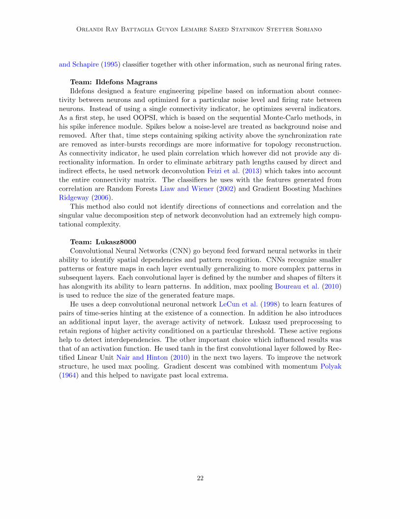
Team: Ildefons MagransIldefons designed a feature engineering pipeline based on information about connec-

tivity between neurons and optimized for a particular noise level and firing rate betweenneurons. Instead of using a single connectivity indicator, he optimizes several indicators.As a first step, he used OOPSI, which is based on the sequential Monte-Carlo methods, inhis spike inference module. Spikes below a noise-level are treated as background noise andremoved. After that, time steps containing spiking activity above the synchronization rateare removed as inter-bursts recordings are more informative for topology reconstruction.As connectivity indicator, he used plain correlation which however did not provide any di-rectionality information. In order to eliminate arbitrary path lengths caused by direct andindirect effects, he used network deconvolution Feizi et al. (2013) which takes into accountthe entire connectivity matrix. The classifiers he uses with the features generated fromcorrelation are Random Forests Liaw and Wiener (2002) and Gradient Boosting MachinesRidgeway (2006).

This method also could not identify directions of connections and correlation and thesingular value decomposition step of network deconvolution had an extremely high compu-tational complexity.

Team: Lukasz8000Convolutional Neural Networks (CNN) go beyond feed forward neural networks in their

ability to identify spatial dependencies and pattern recognition. CNNs recognize smallerpatterns or feature maps in each layer eventually generalizing to more complex patterns insubsequent layers. Each convolutional layer is defined by the number and shapes of filters ithas alongwith its ability to learn patterns. In addition, max pooling Boureau et al. (2010)is used to reduce the size of the generated feature maps.

He uses a deep convolutional neuronal network LeCun et al. (1998) to learn features ofpairs of time-series hinting at the existence of a connection. In addition he also introducesan additional input layer, the average activity of network. Lukasz used preprocessing toretain regions of higher activity conditioned on a particular threshold. These active regionshelp to detect interdependencies. The other important choice which influenced results wasthat of an activation function. He used tanh in the first convolutional layer followed by Rec-tified Linear Unit Nair and Hinton (2010) in the next two layers. To improve the networkstructure, he used max pooling. Gradient descent was combined with momentum Polyak(1964) and this helped to navigate past local extrema.

22

Documents

First Connectomics Challenge: From Imaging to Connectivityproceedings.mlr.press/v46/orlandi15.pdf · Orlandi Ray Battaglia Guyon Lemaire Saeed Statnikov Stetter Soriano methods, including