FIRST ORDER DYNAMIC SYSTEMS

MAPUA INSTITUTE OF TECHNOLOGY

School of Chemical Engineering & Chemistry

Process Control & Instrumentation

4 BASIC COMPONENTS IN A FEEDBACK CONTROL

LOOP

Refining Process (Plant)1. Process

3. Controller

Set Point (SV)

Controlled Variable (CV)

Operator

2. Measuring Element 4. Final Control Element

Process Variable (PV)

Manipulated Variable (MV)

Load Variable

Controller Output

OUTLINE

• General Equation• Transfer Function• Physical Examples• Step Response• Sample Problems

u

GENERAL EQUATION

where:

• u = input variable

• t = time

• K = steady state gain• y = output variable

• y0 = y intercept

y

= time constant

(dy/dt) + y = K(u) + y0

TF

DTF 1

us

Steady State

where:

• us = steady state value of u• ys = steady state value of y

ys(dy/dt) + ys = K(us) + y00 + ys = K(us) + y0

(dy/dt) = 0 during steady state

us

Steady State

ysys = K(us) + y0

u

y

K

y0DTF 1

U(s)

TRANSFER FUNCTIONTransfer Function = ratio of the Laplace Transform of

the output variable to that of the input variable

• Y(s) = Laplace Transform of the DEVIATION VARIABLE Y

Y(s)Y(s)

where:

• U(s) = Laplace Transform of the DEVIATION VARIABLE U

U(s)=

K

(s + 1)DTF 1

DTF 2

DTF 3

DTF 4

(5-3)

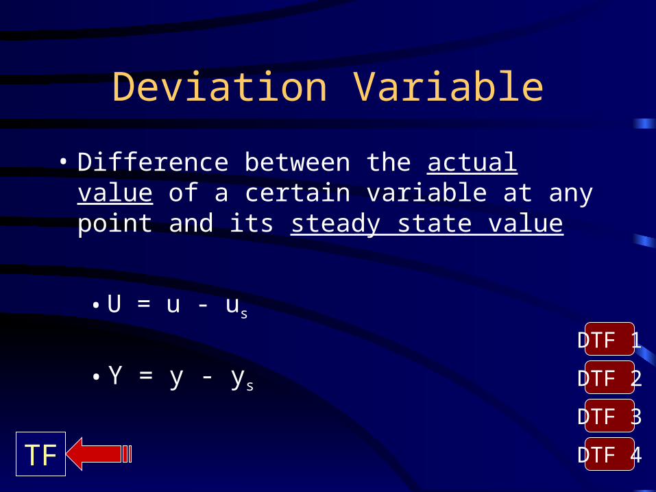
Deviation Variable

• Difference between the actual value of a certain variable at any point and its steady state value

• U = u - us

• Y = y - ys

TF

DTF 1

DTF 2

DTF 3

DTF 4

Deriving the Transfer Function (1/4)

• Subtract the Steady State Equation from the Unsteady State Equation:

(dy/dt) + y = K(u) + y0

ys = K(us) + y0-[

[ ]]

(dy/dt) + (y - ys) = K(u - us) + 0=

Unsteady State

Steady State

TF

DTF 2

DTF 3

DTF 4

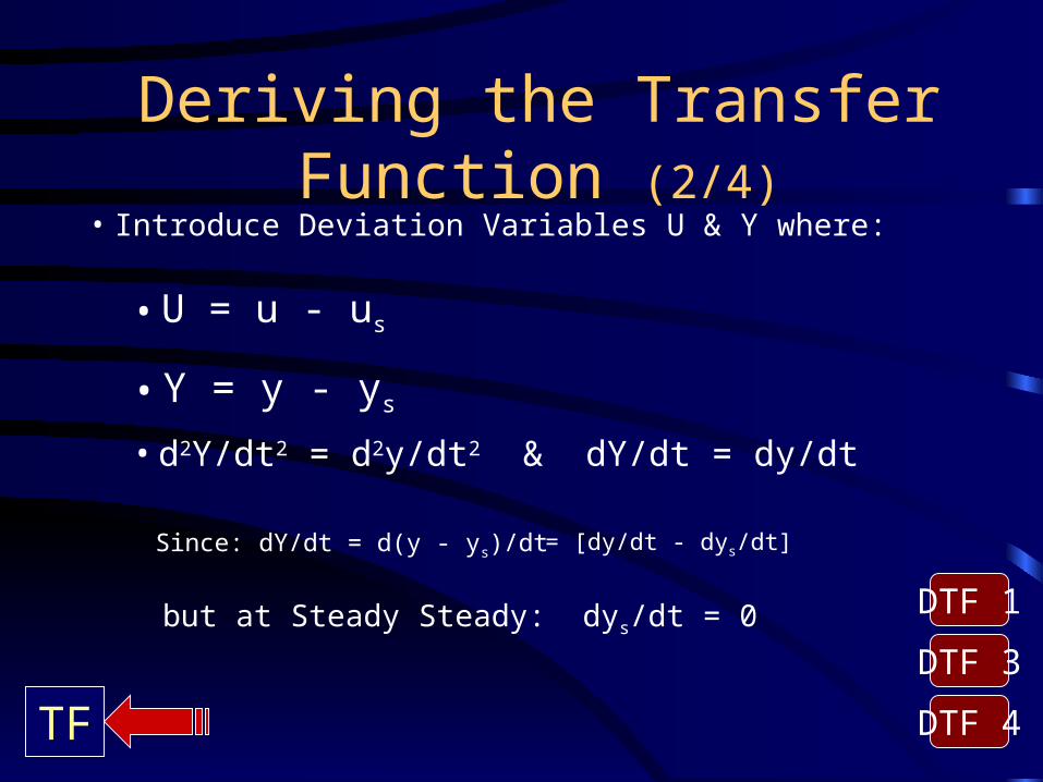
Deriving the Transfer Function (2/4)

• Introduce Deviation Variables U & Y where:

• U = u - us

• Y = y - ys

• dY/dt = dy/dt

Since: dY/dt = d(y - ys)/dt = [dy/dt - dys/dt]

but at Steady Steady: dys/dt = 0

TF

DTF 1

DTF 3

DTF 4

Deriving the Transfer Function (3/4)

• After introducing the Deviation Variables U & Y:

{sY(s) + Y(0)} + Y(s) = K{U(s)}

but at Steady Steady: y = ys therefore Y(0) = 0

sY(s) + Y(s) = K{U(s)}

(dY/dt) + Y = K(U) { }L

TF

DTF 1

DTF 2

DTF 4

Deriving the Transfer Function (4/4)

• Factoring out Y(s):

Y(s){s + 1} = K{U(s)}

• Rearranging:

Y(s)/U(s) = K/{s + 1} Transfer

Function for First Order Systems DTF 1

DTF 2

DTF 3

Step Change in U

0 time, t

u

us

M = magnitude of Step Change

u = us + M

Y(t) = ?

U(t) = M

Example 5.1

(5-4)

Y(t) = MK(1 - e-t/)

Step Response

0 time, t

y

ys

y = ys + MK

Y() = MK

Y = 63.2% of MK

Example 5.1

(5-18)

Y()

• Final Value of Y– value of Y as time t approaches infinity– ultimate value of Y

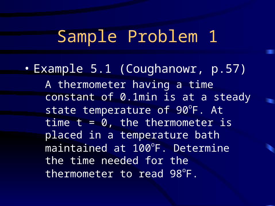
• Example 5.1 (Coughanowr, p.57)A thermometer having a time constant of 0.1min is at a steady state temperature of 90oF. At time t = 0, the thermometer is placed in a temperature bath maintained at 100oF. Determine the time needed for the thermometer to read 98oF.

Sample Problem 1

A well-stirred, continuous mixer has a single input and a single output stream with a variable solute concentration but fixed flow rate. The volume of the mixer is 1000L and the flow rate through it is 500L/min. Initially, the solute concentration is 0.1g/L and it has been constant at this value for a long time. If the inlet concentration were to suddenly increase to 0.15 g/L, and to remain at this new value, how long will it take for the exit concentration to reach 0.125 g/L? Determine the exit concentration 5 minutes after the inlet concentration changed.

Sample Problem 2

SECOND ORDER

DYNAMIC SYSTEMS

MAPUA INSTITUTE OF TECHNOLOGY

School of Chemical Engineering & Chemistry

Process Control & Instrumentation

OUTLINE

• General Equation• Transfer Function• Step Response• Underdamped 2nd Order Systems• Sample Problems

u

GENERAL EQUATION

where:

• u = input variable• K = steady state gain• y = output variable

• y0 = y intercept

y

= time constant

2(d2y/dt2) + 2(dy/dt) + y = K(u) + y0

TF

DTF 1 = damping factor

us

Steady State

where:

• us = steady state value of u

• ys = steady state value of y

ys2(d2y/dt2) + 2(dy/dt) + ys = K(us) + y0 0 + 0 + ys = K(us) + y0

(d2y/dt2)= (dy/dt) = 0 during steady state

us

Steady State

ysys = K(us) + y0

u

y

K

y0DTF 1

U(s)

TRANSFER FUNCTIONTransfer Function = ratio of the Laplace Transform of

the output variable to that of the input variable

• Y(s) = Laplace Transform of the DEVIATION VARIABLE Y

Y(s)Y(s)

where:

• U(s) = Laplace Transform of the DEVIATION VARIABLE U

U(s)=

K

(2s2 + 2s + 1)DTF 1

DTF 2

DTF 3

DTF 4

(5-40)

Deviation Variable

• Difference between the actual value of a certain variable at any point and its steady state value

• U = u - us

• Y = y - ys

TF

DTF 1

DTF 2

DTF 3

DTF 4

Deriving the Transfer Function (1/4)

• Subtract the Steady State Equation from the Unsteady State Equation:

2(d2y/dt 2) + 2(dy/dt) + y = K(u) + y0

ys = K(us) + y0-[

[ ]]

=

Unsteady State

Steady State

TF

DTF 2

DTF 3

DTF 4

2(d2y/dt 2) + 2(dy/dt) + (y - ys) = K(u - us)

Deriving the Transfer Function (2/4)

• Introduce Deviation Variables U & Y where:

• U = u - us

• Y = y - ys

• d2Y/dt2 = d2y/dt2 & dY/dt = dy/dt

Since: dY/dt = d(y - ys)/dt = [dy/dt - dys/dt]

but at Steady Steady: dys/dt = 0

TF

DTF 1

DTF 3

DTF 4

Deriving the Transfer Function (3/4)

• After introducing the Deviation Variables U & Y:

2{s2Y(s) + sY(0) + Y’(0)} + 2{sY(s) - Y(0)} + Y(s) = K{U(s)}

but at Steady Steady: y = ys therefore Y(0) = 0

{ }L

TF

DTF 1

DTF 2

DTF 4

2(d2Y/dt 2) + 2(dY/dt) + Y = K(U)

2s2Y(s) + 2sY(s) + Y(s) = K{U(s)}

Deriving the Transfer Function (4/4)

• Factoring out Y(s):

• Rearranging:

Y(s)/U(s) = K/ {2s2 + 2s + 1} Transfer

Function for Second Order

Systems DTF 1

DTF 2

DTF 3

Y(s){2s2 + 2s + 1} = K{U(s)}

Step Change in U

0 time, t

u

us

M = magnitude of Step Change

u = us + M

Y(t) = ?

U(t) = M

Problem 8.1

(5-4)

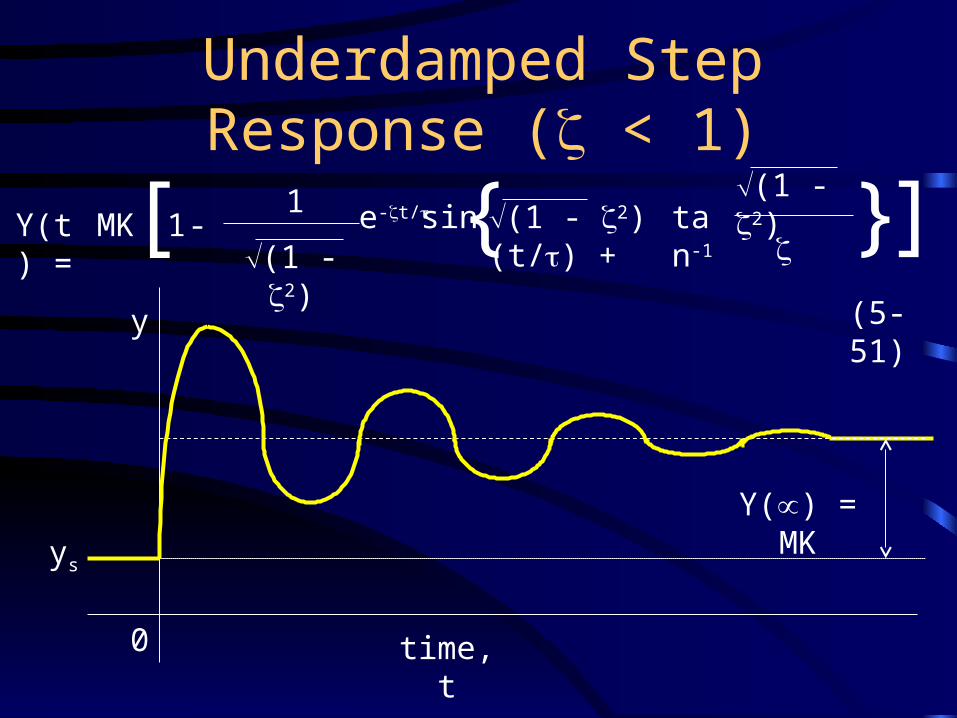
Underdamped Step Response ( < 1)

0 time, t

y

ys Y() = MK

Y(t) = MK1

(1 - 2)- (1 - 2)(t/) +e-t/[1

(1 - 2)

]sin{ }(5-51)

tan-1

Critically Damped Step Response

( = 1)

0 time, t

y

ys

Y() = MK

Y(t) = MKt

+ e-t/[ 1 ]{ }-1 (5-50)

Overdamped Step Response ( > 1)

0 time, t

y

ys

Y() = MK

Y(t) = MK e-t/2[ ]-1 (5-48)2

(2 - 1)}{-e-t/1

1

(1 - 2)}{

= 1

Overdamped Step Response

1 = { + (2 - 1) }

2 = { - (2 - 1) }

Underdamped Step Response ( < 1)

0 time, t

y

ys Y() = MK

BC

tr

Response Time

P

P

Terms Used to Describe an Underdamped 2nd Order Step

Response• Overshoot• Decay Ratio• Rise Time• Response Time• Period of Oscillation

Overshoot

• A measure of how much the response exceeds the ultimate value following a step change.

Overshoot = B/Y()

Overshoot = exp{-/(1 - 2)}(5-53)

Decay Ratio

• The ratio of the sizes of successive peaks.

Decay Ratio = C/B

Decay Ratio = (Overshoot)2 = exp{-2/(1 - 2)} (5-54)

Rise Time (tr)

• The time required for the response to first reach its ultimate value.

tr increases with increasing

Response Time

• The time required for the response to stabilize or to come within +/-5% of its ultimate value.

Period of Oscillation

• The time required to complete one cycle.

Period of Oscillation = 2/(1 - 2) (5-55)

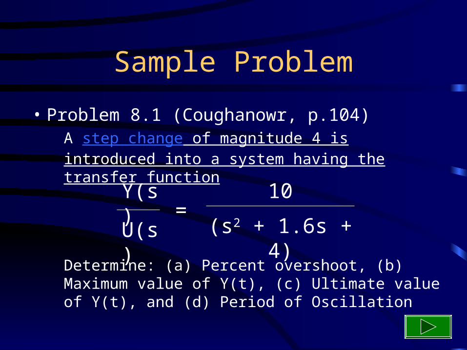
• Problem 8.1 (Coughanowr, p.104)A step change of magnitude 4 is introduced into a system having the transfer function

Determine: (a) Percent overshoot, (b) Maximum value of Y(t), (c) Ultimate value of Y(t), and (d) Period of Oscillation

Sample Problem

Y(s)

U(s)=

10

(s2 + 1.6s + 4)