Embed Size (px)
Citation preview
../ucsbwave-cmyk.png
1
Order Flow Dynamic Order Flow Model Two-Step Approximation Numerical Illustrations
Optimal Execution with Dynamic Order FlowImbalance
Kyle Bechler
UC Santa Barbara
WCMFSeptember 27, 2014
joint w/Mike Ludkovski
Bechler Execution & Order Flow
../ucsbwave-cmyk.png
1
Order Flow Dynamic Order Flow Model Two-Step Approximation Numerical Illustrations
Outline
1 Order Flow
2 Dynamic Order Flow Model
3 Two-Step Approximation
4 Numerical Illustrations
Bechler Execution & Order Flow
../ucsbwave-cmyk.png
2
Order Flow Dynamic Order Flow Model Two-Step Approximation Numerical Illustrations
Tale of Two Costs
When executing a large order in an electronic market, there are twoprimary concerns:
1 Price ImpactSpatial effect: consume liquidity in terms of standing limit orders“Walking through the book” – receive worse price than currentbest bid/ask
2 Information LeakageTemporal effect: executed trade appears on the order tapeOther traders react and adjust their behavior (eg “front-running”) –will receive worse price in the future
Bechler Execution & Order Flow
../ucsbwave-cmyk.png
3
Order Flow Dynamic Order Flow Model Two-Step Approximation Numerical Illustrations
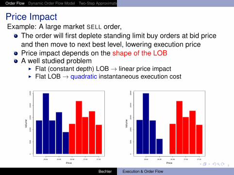
Price ImpactExample: A large market SELL order,
The order will first deplete standing limit buy orders at bid priceand then move to next best level, lowering execution pricePrice impact depends on the shape of the LOBA well studied problem
I Flat (constant depth) LOB→ linear price impactI Flat LOB→ quadratic instantaneous execution cost
26.94 26.96 26.98 27.00 27.02
050
0010
000
1500
020
000
2500
0
Price
Vol
ume
26.94 26.96 26.98 27.00 27.02
050
0010
000
1500
020
000
2500
0
Price
Vol
ume
Bechler Execution & Order Flow
../ucsbwave-cmyk.png
4
Order Flow Dynamic Order Flow Model Two-Step Approximation Numerical Illustrations
Information Leakage
Longer term impact causing others to behave differently (iepermanent market impact)Once other traders are aware of somebody selling, they will takeadvantageAdverse selection, predatory trading, etc.Algorithm should do the following:
I Attempt to hide overall intentionsI Consider the state of the liquidity provision process
Information cost requires looking at time series of orders
Bechler Execution & Order Flow
../ucsbwave-cmyk.png
5
Order Flow Dynamic Order Flow Model Two-Step Approximation Numerical Illustrations
Order Flow
Participants fear that other traders are better informed⇒ When order flow is toxic market makers provide less liquidity
Toxicity is about the ratio of noise/informed traders, aka flowimbalance (NOT the same as static/volume LOB order imbalance)Not directly observable, and not obvious how to measure
Economics: VPIN by Easley, Lopez de Prado, O’Hara (2012abcd)(patented; http://en.wikipedia.org/wiki/Talk:VPIN)
I VPIN has a complicated way of classifying trades as buys/sells. Notsuitable for LOB data
I Claim: MMs widen spreads in response to toxic flowFinMath: Cartea, Jaimungal, Ricci (2011)
I Short term price drift driven by market order arrivalsI Result: MMs shift order placement when market order flow is
one-sided
Bechler Execution & Order Flow
../ucsbwave-cmyk.png
5
Order Flow Dynamic Order Flow Model Two-Step Approximation Numerical Illustrations
Order Flow
Participants fear that other traders are better informed⇒ When order flow is toxic market makers provide less liquidity
Toxicity is about the ratio of noise/informed traders, aka flowimbalance (NOT the same as static/volume LOB order imbalance)Not directly observable, and not obvious how to measureEconomics: VPIN by Easley, Lopez de Prado, O’Hara (2012abcd)(patented; http://en.wikipedia.org/wiki/Talk:VPIN)
I VPIN has a complicated way of classifying trades as buys/sells. Notsuitable for LOB data
I Claim: MMs widen spreads in response to toxic flow
FinMath: Cartea, Jaimungal, Ricci (2011)I Short term price drift driven by market order arrivalsI Result: MMs shift order placement when market order flow is
one-sided
Bechler Execution & Order Flow
../ucsbwave-cmyk.png
5
Order Flow Dynamic Order Flow Model Two-Step Approximation Numerical Illustrations
Order Flow
Participants fear that other traders are better informed⇒ When order flow is toxic market makers provide less liquidity
Toxicity is about the ratio of noise/informed traders, aka flowimbalance (NOT the same as static/volume LOB order imbalance)Not directly observable, and not obvious how to measureEconomics: VPIN by Easley, Lopez de Prado, O’Hara (2012abcd)(patented; http://en.wikipedia.org/wiki/Talk:VPIN)
I VPIN has a complicated way of classifying trades as buys/sells. Notsuitable for LOB data
I Claim: MMs widen spreads in response to toxic flowFinMath: Cartea, Jaimungal, Ricci (2011)
I Short term price drift driven by market order arrivalsI Result: MMs shift order placement when market order flow is
one-sided
Bechler Execution & Order Flow
../ucsbwave-cmyk.png
6
Order Flow Dynamic Order Flow Model Two-Step Approximation Numerical Illustrations
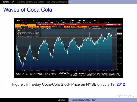
Waves of Coca Cola
Figure : Intra-day Coca-Cola Stock Price on NYSE on July 19, 2012
Bechler Execution & Order Flow
../ucsbwave-cmyk.png
7
Order Flow Dynamic Order Flow Model Two-Step Approximation Numerical Illustrations
Direction
ELO12: Flow imbalance, info leakage and optimal horizonI Static, one-period model
Aim: Incorporate concepts in a dynamic optimal executionframework
I Continuous trading rates (Almgren-Chriss,...)I Assume a parametric form for inventory risk (A-C, Gatheral-Schied)I No fill risk (in contrast to Cartea & Jaimungal, Gueant et al,
Bayraktar-L, ... )I Treat only market orders (in the future: hybrid models like in
Guilbaud & Pham, Carmona & Webster, ... )I (Order book resilience (Obizhaeva & Wang, Alfonsi et al))I (Empirical evidence: Farmer, Bouchaud, ... )
Bechler Execution & Order Flow
../ucsbwave-cmyk.png
8
Order Flow Dynamic Order Flow Model Two-Step Approximation Numerical Illustrations
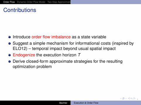
Contributions
Introduce order flow imbalance as a state variableSuggest a simple mechanism for informational costs (inspired byELO12) – temporal impact beyond usual spatial impactEndogenize the execution horizon TDerive closed-form approximate strategies for the resultingoptimization problem
Bechler Execution & Order Flow
../ucsbwave-cmyk.png
9
Order Flow Dynamic Order Flow Model Two-Step Approximation Numerical Illustrations
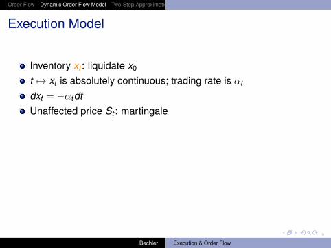
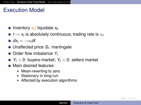
Execution Model
Inventory xt : liquidate x0
t 7→ xt is absolutely continuous; trading rate is αt
dxt = −αtdtUnaffected price St : martingale
Order flow imbalance Yt
Yt > 0: buyers-market; Yt < 0: sellers marketMain desired features:
I Mean-reverting to zeroI Stationary in long-runI Affected by execution algorithms
Bechler Execution & Order Flow
../ucsbwave-cmyk.png
9
Order Flow Dynamic Order Flow Model Two-Step Approximation Numerical Illustrations
Execution Model
Inventory xt : liquidate x0
t 7→ xt is absolutely continuous; trading rate is αt
dxt = −αtdtUnaffected price St : martingaleOrder flow imbalance Yt
Yt > 0: buyers-market; Yt < 0: sellers marketMain desired features:
I Mean-reverting to zeroI Stationary in long-runI Affected by execution algorithms
Bechler Execution & Order Flow
../ucsbwave-cmyk.png
10
Order Flow Dynamic Order Flow Model Two-Step Approximation Numerical Illustrations
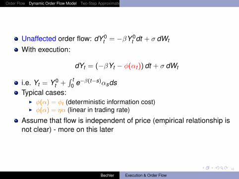
Unaffected order flow: dY 0t = −βY 0
t dt + σ dWt
With execution:
dYt = (−βYt − φ(αt))dt + σ dWt
i.e. Yt = Y 0t +
∫ t0 e−β(t−s)αsds
Typical cases:I φ(α) = φt (deterministic information cost)I φ(α) = ηα (linear in trading rate)
Assume that flow is independent of price (empirical relationship isnot clear) - more on this later
Bechler Execution & Order Flow
../ucsbwave-cmyk.png
11
Order Flow Dynamic Order Flow Model Two-Step Approximation Numerical Illustrations
Optimization Problem
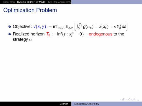
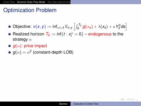
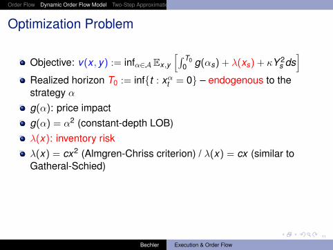
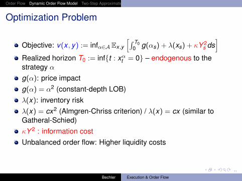
Objective: v(x , y) := infα∈A Ex ,y
[∫ T00 g(αs) + λ(xs) + κY 2
s ds]
Realized horizon T0 := inf{t : xαt = 0} – endogenous to thestrategy α
g(α): price impact
g(α) = α2 (constant-depth LOB)
λ(x): inventory risk
λ(x) = cx2 (Almgren-Chriss criterion) / λ(x) = cx (similar toGatheral-Schied)
κY 2 : information cost
Unbalanced order flow: Higher liquidity costs
Bechler Execution & Order Flow
../ucsbwave-cmyk.png
11
Order Flow Dynamic Order Flow Model Two-Step Approximation Numerical Illustrations
Optimization Problem
Objective: v(x , y) := infα∈A Ex ,y
[∫ T00 g(αs) + λ(xs) + κY 2
s ds]
Realized horizon T0 := inf{t : xαt = 0} – endogenous to thestrategy αg(α): price impactg(α) = α2 (constant-depth LOB)
λ(x): inventory risk
λ(x) = cx2 (Almgren-Chriss criterion) / λ(x) = cx (similar toGatheral-Schied)
κY 2 : information cost
Unbalanced order flow: Higher liquidity costs
Bechler Execution & Order Flow
../ucsbwave-cmyk.png
11
Order Flow Dynamic Order Flow Model Two-Step Approximation Numerical Illustrations
Optimization Problem
Objective: v(x , y) := infα∈A Ex ,y
[∫ T00 g(αs) + λ(xs) + κY 2
s ds]
Realized horizon T0 := inf{t : xαt = 0} – endogenous to thestrategy αg(α): price impactg(α) = α2 (constant-depth LOB)λ(x): inventory riskλ(x) = cx2 (Almgren-Chriss criterion) / λ(x) = cx (similar toGatheral-Schied)
κY 2 : information cost
Unbalanced order flow: Higher liquidity costs
Bechler Execution & Order Flow
../ucsbwave-cmyk.png
11
Order Flow Dynamic Order Flow Model Two-Step Approximation Numerical Illustrations
Optimization Problem
Objective: v(x , y) := infα∈A Ex ,y
[∫ T00 g(αs) + λ(xs) + κY 2
s ds]
Realized horizon T0 := inf{t : xαt = 0} – endogenous to thestrategy αg(α): price impactg(α) = α2 (constant-depth LOB)λ(x): inventory riskλ(x) = cx2 (Almgren-Chriss criterion) / λ(x) = cx (similar toGatheral-Schied)κY 2 : information costUnbalanced order flow: Higher liquidity costs
Bechler Execution & Order Flow
../ucsbwave-cmyk.png
12
Order Flow Dynamic Order Flow Model Two-Step Approximation Numerical Illustrations
HJB Equation
0 = −βYvY + 12σ
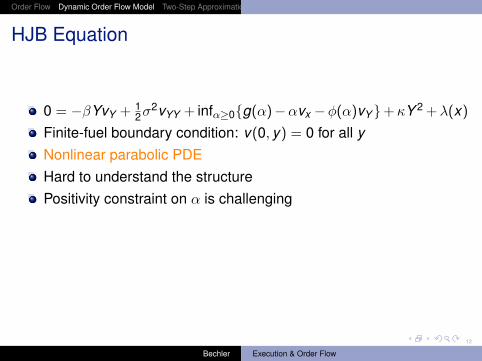
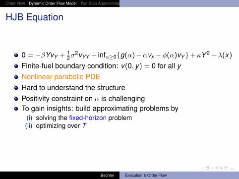
2vYY + infα≥0{g(α)−αvx −φ(α)vY}+κY 2 +λ(x)Finite-fuel boundary condition: v(0, y) = 0 for all yNonlinear parabolic PDEHard to understand the structurePositivity constraint on α is challenging
To gain insights: build approximating problems by(i) solving the fixed-horizon problem(ii) optimizing over T
Bechler Execution & Order Flow
../ucsbwave-cmyk.png
12
Order Flow Dynamic Order Flow Model Two-Step Approximation Numerical Illustrations
HJB Equation
0 = −βYvY + 12σ
2vYY + infα≥0{g(α)−αvx −φ(α)vY}+κY 2 +λ(x)Finite-fuel boundary condition: v(0, y) = 0 for all yNonlinear parabolic PDEHard to understand the structurePositivity constraint on α is challengingTo gain insights: build approximating problems by
(i) solving the fixed-horizon problem(ii) optimizing over T
Bechler Execution & Order Flow
../ucsbwave-cmyk.png
13
Order Flow Dynamic Order Flow Model Two-Step Approximation Numerical Illustrations
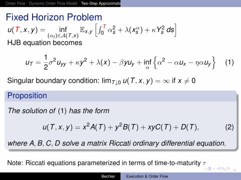
Fixed Horizon Problemu(T , x , y) = inf
(αt )∈A(T ,x)Ex ,y
[∫ T0 α2
s + λ(xαs ) + κY 2s ds
]HJB equation becomes
uT =12σ2uyy + κy2 + λ(x)− βyuy + inf
α
{α2 − αux − ηαuy
}(1)
Singular boundary condition: limT↓0 u(T , x , y) =∞ if x 6= 0
Proposition
The solution of (1) has the form
u(T , x , y) = x2A(T ) + y2B(T ) + xyC(T ) + D(T ), (2)
where A,B,C,D solve a matrix Riccati ordinary differential equation.
Note: Riccati equations parameterized in terms of time-to-maturity τ
Bechler Execution & Order Flow
../ucsbwave-cmyk.png
14
Order Flow Dynamic Order Flow Model Two-Step Approximation Numerical Illustrations
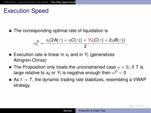
Execution Speed
The corresponding optimal rate of liquidation is
αDt =
xt(2A(τ) + ηC(τ)) + Yt(C(τ) + 2ηB(τ))
2.
Execution rate is linear in xt and in Yt (generalizesAlmgren-Chriss)The Proposition only treats the unconstrained case α ∈ R: if T islarge relative to x0 or Yt is negative enough then αD < 0As t → T , the dynamic trading rate stabilizes, resembling a VWAPstrategy.
Bechler Execution & Order Flow
../ucsbwave-cmyk.png
15
Order Flow Dynamic Order Flow Model Two-Step Approximation Numerical Illustrations
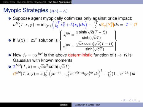
Myopic Strategies (φ(α) = φt )
Suppose agent myopically optimizes only against price impact:uM(T , x , y) := inf(xt )
(∫ T0 x2
s + λ(xs)ds)+∫ T
0 κEy [Y 2s ]ds =: I +O
If λ(x) = cx2 solution is
xMH
t =x sinh(
√c(T − t))
sinh(√
cT )
αMHt =
√cx cosh(
√c(T − t))
sinh(√
cT )
Now φt = ηαMH
t is the above deterministic function of t → Yt isGaussian with known momentsIMH(T , x) =
√cx2 coth(
√cT )
OMH(T , x , y) = κ∫ T
0
(ye−βt −
∫ t0 e−β(t−s)ηαMH
s ds)2
+ σ2
2β (1− e−2βt)dt
Similarly have closed-form expressions for cases λ(x) = cx(Quadratic) and λ(x) = 0 (VWAP)Next step: Take existing closed-form expressions uM and optimizeover T
Bechler Execution & Order Flow
../ucsbwave-cmyk.png
15
Order Flow Dynamic Order Flow Model Two-Step Approximation Numerical Illustrations
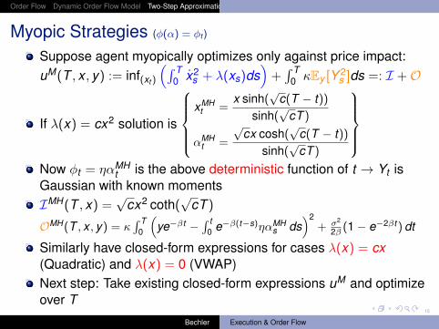
Myopic Strategies (φ(α) = φt )
Suppose agent myopically optimizes only against price impact:uM(T , x , y) := inf(xt )
(∫ T0 x2
s + λ(xs)ds)+∫ T
0 κEy [Y 2s ]ds =: I +O
If λ(x) = cx2 solution is
xMH
t =x sinh(
√c(T − t))
sinh(√
cT )
αMHt =
√cx cosh(
√c(T − t))
sinh(√
cT )
Now φt = ηαMH
t is the above deterministic function of t → Yt isGaussian with known momentsIMH(T , x) =
√cx2 coth(
√cT )
OMH(T , x , y) = κ∫ T
0
(ye−βt −
∫ t0 e−β(t−s)ηαMH
s ds)2
+ σ2
2β (1− e−2βt)dt
Similarly have closed-form expressions for cases λ(x) = cx(Quadratic) and λ(x) = 0 (VWAP)Next step: Take existing closed-form expressions uM and optimizeover T
Bechler Execution & Order Flow
../ucsbwave-cmyk.png
16
Order Flow Dynamic Order Flow Model Two-Step Approximation Numerical Illustrations
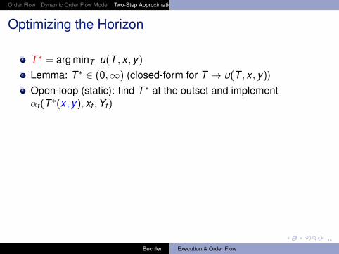
Optimizing the Horizon
T ∗ = arg minT u(T , x , y)Lemma: T ∗ ∈ (0,∞) (closed-form for T 7→ u(T , x , y))Open-loop (static): find T ∗ at the outset and implementαt(T ∗(x , y), xt ,Yt)
Closed-loop (dynamic): continuously recompute T ∗:
αMt (x , y) := αM(T ∗(xt ,Yt), xt ,Yt)
Realized horizon T0(x , y) becomes randomDynamically recomputing T ∗ - adapt to changing Yt without theindefinite horizon finite-fuel problem
Next up: we show these are in fact good approximations!
Bechler Execution & Order Flow
../ucsbwave-cmyk.png
16
Order Flow Dynamic Order Flow Model Two-Step Approximation Numerical Illustrations
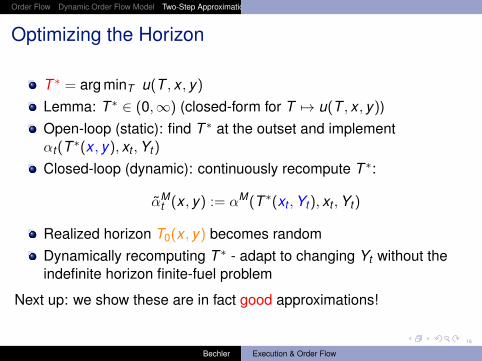
Optimizing the Horizon
T ∗ = arg minT u(T , x , y)Lemma: T ∗ ∈ (0,∞) (closed-form for T 7→ u(T , x , y))Open-loop (static): find T ∗ at the outset and implementαt(T ∗(x , y), xt ,Yt)
Closed-loop (dynamic): continuously recompute T ∗:
αMt (x , y) := αM(T ∗(xt ,Yt), xt ,Yt)
Realized horizon T0(x , y) becomes randomDynamically recomputing T ∗ - adapt to changing Yt without theindefinite horizon finite-fuel problem
Next up: we show these are in fact good approximations!
Bechler Execution & Order Flow
../ucsbwave-cmyk.png
17
Order Flow Dynamic Order Flow Model Two-Step Approximation Numerical Illustrations
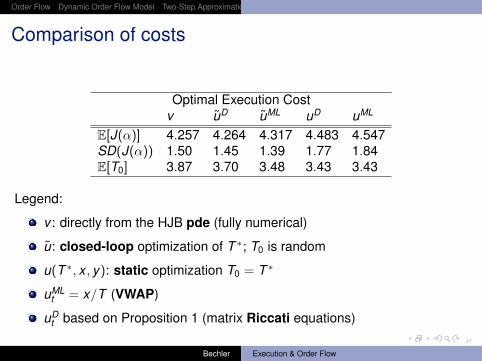
Comparison of costs
Optimal Execution Costv uD uML uD uML
E[J(α)] 4.257 4.264 4.317 4.483 4.547SD(J(α)) 1.50 1.45 1.39 1.77 1.84E[T0] 3.87 3.70 3.48 3.43 3.43
Legend:
v : directly from the HJB pde (fully numerical)
u: closed-loop optimization of T ∗; T0 is random
u(T ∗, x , y): static optimization T0 = T ∗
uMLt = x/T (VWAP)
uDt based on Proposition 1 (matrix Riccati equations)
Bechler Execution & Order Flow
../ucsbwave-cmyk.png
18
Order Flow Dynamic Order Flow Model Two-Step Approximation Numerical Illustrations
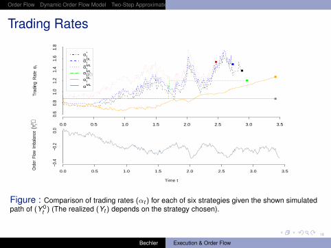
Trading Rates
0.0 0.5 1.0 1.5 2.0 2.5 3.0 3.5
Trad
ing
Rat
e α
t
αt*
α~tDL
α~tML
α(2)ML
αtDL
αML
0.6
0.8
1.0
1.2
1.4
1.6
1.8
0.0 0.5 1.0 1.5 2.0 2.5 3.0 3.5
Time t
Ord
er F
low
Imba
lanc
e (Y
t0 )
−0.4
−0.2
0.0
Figure : Comparison of trading rates (αt ) for each of six strategies given the shown simulatedpath of (Y 0
t ) (The realized (Yt ) depends on the strategy chosen).
Bechler Execution & Order Flow
../ucsbwave-cmyk.png
19
Order Flow Dynamic Order Flow Model Two-Step Approximation Numerical Illustrations
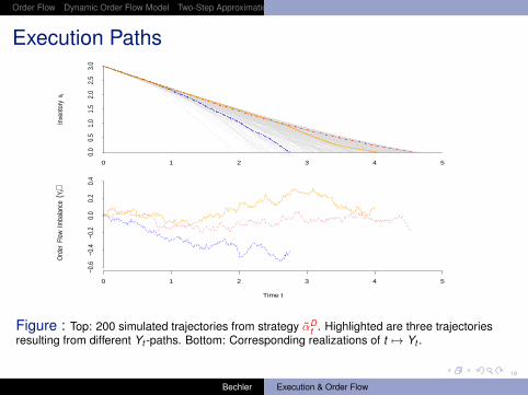
Execution PathsIn
vent
ory
x t
0 1 2 3 4 5
0.0
0.5
1.0
1.5
2.0
2.5
3.0
0 1 2 3 4 5
Time t
Ord
er F
low
Imba
lanc
e (Y
t)
−0.6
−0.4
−0.2
0.0
0.2
0.4
Figure : Top: 200 simulated trajectories from strategy αDt . Highlighted are three trajectories
resulting from different Yt -paths. Bottom: Corresponding realizations of t 7→ Yt .
Bechler Execution & Order Flow
../ucsbwave-cmyk.png
20
Order Flow Dynamic Order Flow Model Two-Step Approximation Numerical Illustrations
More on Static T ∗ (Optimal Execution Horizon byELO12)
ELO12 (essentially) considered minT≥0{Ex ,y [|YαT |] + c
√T}
⇒ myopic trading based on constant participation strategy αt = x/T ;explicit timing costs (rather than inventory risk)Only terminal information costs |YT |Discuss the statically optimized T ∗ aboveOur setup is effectively a dynamic extension of the aboveone-period model
Bechler Execution & Order Flow
../ucsbwave-cmyk.png
21
Order Flow Dynamic Order Flow Model Two-Step Approximation Numerical Illustrations
Work in Progress
http://arxiv.org/abs/1409.2618
Empirical measurement of order flow and its stylized featuresAt what time-scale is order flow imbalance to be measured?Perhaps information leakage φ(α) depends on Yt?Consider correlated St and Yt
Thank You!
Bechler Execution & Order Flow
../ucsbwave-cmyk.png
22
Order Flow Dynamic Order Flow Model Two-Step Approximation Numerical Illustrations
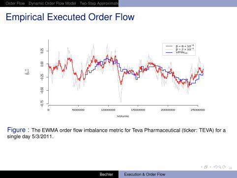
Empirical Executed Order Flow
0 500000 1000000 1500000 2000000 2500000
Volume
(I k)
−0.7
5−0
.50
−0.2
50.
000.
25β = 8 × 10⁻⁶
β = 2 × 10⁻⁵
VPIN10
Figure : The EWMA order flow imbalance metric for Teva Pharmaceutical (ticker: TEVA) for asingle day 5/3/2011.
Bechler Execution & Order Flow
../ucsbwave-cmyk.png
23
Order Flow Dynamic Order Flow Model Two-Step Approximation Numerical Illustrations
References
R. Cont, A. Kukanov and S. StoikovThe price impact of order book eventshttp://papers.ssrn.com/sol3/papers.cfm?abstract_id=1712822 (2012)
D. Easley, M. López de Prado and M. O’HaraFlow Toxicity and Liquidity in a High Frequency WorldReview of Financial Studies, (2012) 25, 1457–1493.
D. Easley, M. López de Prado and M. O’HaraOptimal Execution Horizonhttp://papers.ssrn.com/sol3/papers.cfm?abstract_id=2038387 (2012)
J. Gatheral and A. SchiedDynamical models of market impact and algorithms for order executionhttp://papers.ssrn.com/sol3/papers.cfm?abstract_id=2034178 (2013)
A. Cartea, S. Jaimungal and J. RicciBuy low sell high: a high frequency trading perspectivehttp://papers.ssrn.com/sol3/papers.cfm?abstract_id=1964781 (2011)
Bechler Execution & Order Flow