Embed Size (px)
Citation preview
Geophys. J. Int. (2007) 171, 368–389 doi: 10.1111/j.1365-246X.2007.03528.xG
JISei
smol
ogy
Finite-frequency sensitivity of body waves to anisotropy based uponadjoint methods
Anne Sieminski,1 Qinya Liu,2 Jeannot Trampert1 and Jeroen Tromp2
1Department of Earth Sciences, Utrecht University, PO Box 80021, TA 3058 Utrecht, the Netherlands. E-mail: [email protected] Laboratory, California Institute of Technology, Pasadena, CA 91125, USA
Accepted 2007 June 20. Received 2007 June 15; in original form 2007 March 19
S U M M A R YWe investigate the sensitivity of finite-frequency body-wave observables to mantle anisotropybased upon kernels calculated by combining adjoint methods and spectral-element modellingof seismic wave propagation. Anisotropy is described by 21 density-normalized elastic param-eters naturally involved in asymptotic wave propagation in weakly anisotropic media. In a 1-Dreference model, body-wave sensitivity to anisotropy is characterized by ‘banana–doughnut’kernels which exhibit large, path-dependent variations and even sign changes. P-wave travel-times appear much more sensitive to certain azimuthally anisotropic parameters than to theusual isotropic parameters, suggesting that isotropic P-wave tomography could be significantlybiased by coherent anisotropic structures, such as slabs. Because of shear-wave splitting, thecommon cross-correlation traveltime anomaly is not an appropriate observable for S wavespropagating in anisotropic media. We propose two new observables for shear waves. The firstobservable is a generalized cross-correlation traveltime anomaly, and the second a general-ized ‘splitting intensity’. Like P waves, S waves analysed based upon these observables aregenerally sensitive to a large number of the 21 anisotropic parameters and show significantpath-dependent variations. The specific path-geometry of SKS waves results in favourableproperties for imaging based upon the splitting intensity, because it is sensitive to a smallernumber of anisotropic parameters, and the region which is sampled is mainly limited to theupper mantle beneath the receiver.
Key words: adjoint methods, body waves, Frechet derivatives, seismic anisotropy, sensitivity,shear-wave splitting.
1 I N T RO D U C T I O N
Seismic anisotropy is an essential property of the elastic structure of the mantle. Many mantle minerals are anisotropic (Mainprice et al. 2000)and can be preferentially oriented by large-scale flow and deformation (Kaminski & Ribe 2002). It is therefore crucial to take anisotropy intoaccount when imaging the mantle. Comparing combined modelling in geodynamics and mineral physics with 3-D maps of seismic anisotropyprovides unique information about mantle dynamics and tectonic processes (Becker et al. 2006). The first body-wave signature of mantleanisotropy was found in azimuthal variations of Pn-wave speeds in oceanic regions (Hess 1964). Teleseismic P-wave residuals have also beenused to constrain anisotropy (Gresillaud & Cara 1996; Plomerova et al. 1996). However, recently, the most popular method to map anisotropyfrom body-wave observations has been to exploit shear-wave splitting. Being radially polarized in isotropic earth models, SKS waves areespecially well suited to this approach, and several techniques have been proposed to measure SKS splitting (Silver & Chan 1988; Vinniket al. 1989; Savage 1999; Chevrot 2000).
Body-wave studies of anisotropy are usually based on an asymptotic description of wave propagation (i.e. ray theory). Asymptoticbody-wave propagation in weakly anisotropic models is well developed (Jech & Psencık 1989; Farra 2001; Chen & Tromp 2007). There isfirm belief that significant progress in imaging Earth structure requires consideration of the finite-frequency aspects of wave propagation. Thishas motivated the development of numerical and analytical methods to calculate finite-frequency Frechet derivatives, or sensitivity kernels,representing changes in seismic observables due to changes in structure (Marquering et al. 1999; Dahlen et al. 2000; Zhao et al. 2005; Zhao& Jordan 2006). Thus far, the application of these methods to compute sensitivity kernels has been limited to isotropic structures, and it isnot well understood how finite-frequency seismic observables ‘sense’ anisotropy. For example, the precise region sampled by SKS-splittingmeasurements is still uncertain. SKS splitting is usually assumed to provide excellent lateral resolution but limited vertical resolution. Much ofthe interpretation consists of determining where the anisotropy should be located in depth (Alsina & Snieder 1995; Silver 1996; Savage 1999).
368 C© 2007 The Authors
Journal compilation C© 2007 RAS
Finite-frequency sensitivity of body waves 369
Recently, Favier & Chevrot (2003) have provided some answers to this question. They applied Born-scattering theory, using a plane-waveformalism, to analytically describe the sensitivity kernels of Chevrot’s (2000) ‘splitting intensity’ for SKS waves.
An alternative, but more general, approach to calculating the sensitivity of seismic waves to any structural parameter involves thecombination of adjoint methods with spectral-element modelling of seismic wave propagation (Tromp et al. 2005; Liu & Tromp 2006, 2007).This approach has proven to be a powerful tool to numerically compute sensitivity kernels in any 3-D earth model. In a previous paper(Sieminski et al. 2007), we used this tool to investigate the sensitivity to anisotropy of fundamental-mode surface waves. We continue thiswork for body waves in this paper.
We explain in Section 2 how we parametrize anisotropy and briefly review the adjoint spectral-element method for the computation ofanisotropic sensitivity kernels. In Section 3, we define the P- and S-wave traveltime observables before discussing their sensitivity kernels fordirect waves at teleseismic distances. The specific example of SKS splitting is addressed in Section 4, before concluding.
2 A N I S O T RO P Y A N D A D J O I N T S P E C T R A L - E L E M E N T S E N S I T I V I T Y K E R N E L S
2.1 Parametrization of anisotropy
The elastic structure of the mantle is described by a fourth-order elastic tensor relating the strain to the stress, whose components are denotedcijkl, i , j , k, l = 1, 2, 3. Due to symmetry properties, the elastic tensor has only 21 independent components (e.g. Babuska & Cara 1991). Toassess the effects of anisotropy, we must thus analyse the sensitivity to 21 model parameters. These 21 independent components of the elastictensor may be rewritten using Voigt’s notation with contracted indices as C IJ , I , J = 1, . . . , 6 (e.g. Babuska & Cara 1991). The definition ofthe parameters C IJ in terms of the corresponding elements cijkl of the elastic tensor in spherical coordinates is given in Appendix A. Specificcombinations of these C IJ appear naturally when considering asymptotic wave propagation. In this approximation, an anisotropic perturbationin surface-wave phase speed is determined by an even Fourier series in ξ , the local azimuth. As first demonstrated by Smith & Dahlen (1973),this series involves degrees zero, two and four. Montagner & Nataf (1986) and Larson et al. (1998) expressed the coefficients of the seriesin terms of a linear combination of perturbations of the C IJ for plane and spherical layercake models, respectively. The five parametersassociated with degree zero are the perturbations of the Love parameters {A, C, N , L, F} (Love 1911) corresponding to transverse isotropy(Appendix B). The azimuthal variation of surface waves is controlled by the parameters {B c,s , H c,s , G c,s} for the 2-ξ variations and {E c,s}for the 4-ξ variations, where the subscripts ‘c’ and ‘s’ refer to a cos nξ or sin nξ , n = 2, 4, dependence, respectively. Anisotropic surface-wave tomography usually describes the model in terms of the Love parameters and the eight azimuthal parameters. Jech & Psencık (1989)demonstrated that asymptotic body-wave propagation in weakly anisotropic media is similarly governed by a Fourier series in ξ involvingdegrees zero, two and four, but also degrees one and three. Chen & Tromp (2007) expanded on Jech & Psencık’s (1989) formulation. In additionto the previous 13 parameters for the 0-ξ , 2-ξ and 4-ξ dependence, they introduced eight new elastic parameters {J c,s , K c,s , M c,s} and {Dc,s}corresponding to linear combinations of C IJ describing the 1-ξ and 3-ξ variations, respectively. The five transversely isotropic parameters,the eight azimuthal surface-wave parameters, and the additional eight azimuthal body-wave parameters define a complete parametrizationof a general anisotropic medium. In the following, we will refer to these parameters as the ‘Chen & Tromp’ parameters. The relationshipbetween the Chen & Tromp parameters and the C IJ is given in Appendix A. Tromp et al. (2005) and Liu & Tromp (2006) showed thatseismic traveltimes are more efficiently described by wave speeds rather than elastic parameters and density. In this study, we are interestedin traveltime observables, and, therefore, we chose to analyse the sensitivity to the squared wave speeds associated with the Chen & Trompparameters. These 21 anisotropic squared wave speeds are simply the density-normalized elastic parameters. We denote them with a prime, forexample A′ = A/ρ. When studying anisotropy, seismologists often assume transverse isotropy. Only five elastic parameters are needed in thiscase. A transversely isotropic structure with a vertical symmetry axis may be described by the speeds αh , αv , β h , βv and the dimensionlessparameter η (Section B1 of Appendix B). The Preliminary Reference Earth Model (PREM, Dziewonski & Anderson 1981) is a widely usedexample of a transversely isotropic earth model with a vertical symmetry axis. The sensitivity to these transversely isotropic parameters willbe discussed as well.
2.2 Adjoint spectral-element method
Adjoint methods were introduced in seismic imaging by Tarantola (1984) for acoustic waves and by Tarantola (1987, 1988) for elastic waves.Recently, Tromp et al. (2005) drew connections between this method and finite-frequency (‘banana–doughnut’) sensitivity kernels (Marqueringet al. 1999; Dahlen et al. 2000). Based on this work, Tape et al. (2007) proposed a strategy for ‘adjoint tomography’. We will briefly summarizethe basis of Tromp et al.’s (2005) approach. Details regarding the mathematical aspects of adjoint methods and sensitivity kernels may alsobe found in Liu & Tromp (2006, 2007). In this study, we are interested in the kernels that describe, in a Born-scattering formalism, how afirst-order perturbation of a model parameter affects a seismic observable. Tromp et al. (2005) demonstrated that the sensitivity kernels K δcjklm
for a perturbation of the elastic parameters δcjklm at location x may be expressed as the interaction between a regular displacement wavefields, propagating from the source to the receiver, and an ‘adjoint’ wavefield s†, which propagates from the receiver to the source:
Kδc jklm (x) = −∫ T
0e†jk(x, T − t)elm(x, t) dt, (1)
C© 2007 The Authors, GJI, 171, 368–389
Journal compilation C© 2007 RAS
370 A. Sieminski et al.
where t denotes time, [0, T] the time interval of interest, and e†jk and elm the components of the strain tensors associated with the adjointwavefield s† and regular wavefield s, respectively. The definition of the adjoint wavefield is intimately linked to the type of observable underconsideration. Most seismic observables are constructed from the difference between observed and synthetic waveforms. They are expressedin terms of perturbations in displacement as
oi =∫ T
0ψi (xr , t)δsi (xr , t) dt (no summation over i), (2)
where oi denotes the observable, δs i the ith component of the perturbed displacement field, xr the receiver position and ψ i a functiondetermined by the kind of observable. The adjoint wavefield corresponding to the observable oi is generated at the receiver by the adjointsource
f †i (x, t) = ψi (xr , T − t)δ(x − xr ). (3)
In this paper, we calculate the wavefields s and s† with the spectral-element method developed by Komatitsch & Vilotte (1998) and furtherextended for global wave propagation in anisotropic models including 3-D crustal & mantle models, ellipticity topography and bathymetry,oceans, the Earth’s rotation and self-gravitation (Komatitsch & Tromp 2002a,b; Chen & Tromp 2007). The numerical implementation of theadjoint spectral-element method to calculate sensitivity kernels is detailed by Liu & Tromp (2006) for regional-scale problems and by Liu &Tromp (2007) at the scale of the globe. Other numerical methods can be used to simulate wave propagation and compute kernels. For example,Zhao et al. (2005) used a finite-difference method to calculate regional-scale, isotropic sensitivity kernels. Several analytical approaches havebeen developed to compute finite-frequency isotropic sensitivity kernels. For example, Dahlen et al. (2000) used a ray-based method, whileZhao & Jordan (2006) adopted a full-wave approach based upon a normal-mode formalism. With numerical methods, such as spectral-elementand finite-difference techniques, we can efficiently compute the sensitivity of any seismic observable, written in the form of eq. (2), for anyportion of the seismogram, for the full wavefield. We are not limited to the few seismic arrivals defined by classical ray theory. Normal-modemethods (e.g. Zhao & Jordan 2006) have the same advantage but, contrary to analytical approaches, numerical methods do not require 1-Dreference models, they can calculate sensitivity kernels in any 3-D model.
The computation of sensitivity kernels with the adjoint spectral-element method requires one forward simulation to build the adjointsource (eq. 3), and a combined forward and adjoint simulation to construct the kernels according to eq. (1). The results of this approach arekernels that reflect the sensitivity to anisotropic model perturbations δcjklm. We combine these ‘primary’ kernels to obtain kernels for theChen & Tromp parameters (Appendix A). The sensitivity kernels for the squared anisotropic wave speeds are then simply proportional to theelastic kernels, for example, K δA′ = ρK δA (Sieminski et al. 2007). Kernels for isotropic parameters (such as the isotropic P-wave speed α
and S-wave speed β) may be obtained by combining the anisotropic kernels according to eqs (B5) and (B6). This gives results in agreementwith the isotropic kernels of Zhao et al. (2005), Hung et al. (2000) and Liu & Tromp (2006, 2007), who calculated isotropic kernels directlyfrom the interaction between the regular and adjoint wavefields (eqs 17, 18 and 20 of Tromp et al. 2005).
In the next section we apply the adjoint spectral-element method to compute sensitivity kernels for teleseismic P and S waves. We will seethat S waves require the introduction of specific observables, and we will define a generalized traveltime anomaly and a generalized ‘splittingintensity’. Because the physical interpretation of S-wave sensitivity is not straightforward, we initially divide the S-wave analysis into pureSV - and SH-wave cases. These experiments allow us to describe the general sensitivity of body waves to anisotropy.
3 P - A N D S - WAV E S E N S I T I V I T Y
3.1 P wave
3.1.1 P-wave observable and adjoint source definition
The common observable for isotropic imaging is the traveltime anomaly δT of the selected wave relative to its theoretical arrival time in thereference model. It is often measured by cross-correlation between the observed signal d and the synthetic signal s calculated in the referencemodel. This technique assumes a small perturbation, that is, the traveltime anomaly is assumed to be small compared to the period of thesignal and the waveform of the observed pulse is similar to the synthetic one. The approach can be applied to study anisotropic quasi-P wavesbased upon an isotropic reference model, because P waveforms are only slightly affected by weak anisotropy (Chen & Tromp 2007). Usingthe notation of Jech & Psencık (1989) and Chen & Tromp (2007), we write the reference isotropic P-wave signal as
s(x, t) = s3(x, t) e3, (4)
where e3 denotes the unit vector corresponding to the P-wave polarization. The quasi-P-wave polarization is usually very close to the isotropicP-wave polarization (e.g. Farra 2001). The anisotropic quasi-P wave recorded at the receiver xr is thus to first order
d(xr , t) = s3(xr , t − δT3) e3 � [s3(xr , t) − δT3 s3(xr , t)] e3 = [s3(xr , t) + δs3(xr , t)] e3, (5)
where we have defined
δs3 = −δT3 s3, (6)
C© 2007 The Authors, GJI, 171, 368–389
Journal compilation C© 2007 RAS
Finite-frequency sensitivity of body waves 371
and where δT 3 denotes the P-wave traveltime anomaly and s3 the time derivative of the displacement. We use the convention of a positivetraveltime anomaly δT for a delay of the observed pulse relative to the synthetic one. The cross-correlation between the synthetic and observedP-wave signals,
3(τ ) =∫
s3(xr , t − τ )d3(xr , t) dt, (7)
reaches its maximum for τ � δT 3, where (Marquering et al. 1999; Dahlen et al. 2000; Tromp et al. 2005)
δT3 = − 1
N3
∫s3(xr , t)δs3(xr , t) dt. (8)
The normalization factor N 3 is defined by N3 = ∫s2
3 dt , and the time integral is over the P-wave time window. According to eqs (2) and (3),the adjoint source function associated with δT 3 is (Tromp et al. 2005)
f†3 (x, t) = − 1
N3s3(xr , T − t)δ(x − xr ) e3. (9)
3.1.2 P-wave adjoint kernels
We analyse P-wave adjoint sensitivity kernels for the squared wave speeds derived from the Chen & Tromp parameters. Throughout this study,the synthetic seismograms from which the adjoint sources are built are computed by spectral-element simulation (Section 2) in sphericallysymmetric, isotropic PREM (Dziewonski & Anderson 1981). For the P-wave analysis, the source is a vertical point force located at the SouthPole at 600 km depth, the source–time function is a Gaussian with a half duration of 11 s, and the epicentral distance is 75◦. To compute theadjoint source function we low-pass filter the seismograms with a corner at 14.5 s to limit the high-frequency signal in the adjoint wavefield.The time window used to isolate the wave of interest is a Welch taper defined as w(t) = 1 − (2t/�t − 1)2, with �t the width of the time-window(Press et al. 1992). The P-wave traveltime anomaly δT 3 is usually measured from vertical-component recordings. We follow this simplificationhere and consider a purely vertical adjoint source function f†3 . The adjoint source–time function and the selected vertical synthetic signal areshown in Fig. 1. We obtain very similar results if we use the signal on the P-wave polarization direction rather than the vertical component.Only the kernels for the azimuthally anisotropic ‘c-parameters’ (J ′
c, K ′c, M ′
c, B ′c, H ′
c, G ′c, D′
c and E ′c) are shown in Fig. 2, because the kernels
for the ‘s-parameters’ (J ′s , K ′
s , M ′s , B ′
s , H ′s , G ′
s , D′s and E ′
s) have the same characteristics. To avoid clutter, we will drop the subscripts c ands in the following, unless needed. The kernels are displayed in a vertical section throughout the mantle in the source–receiver great-circleplane. In this plane, the kernels for isotropic model perturbations are ‘banana’ shaped (Fig. 3), while a vertical section orthogonal to this planewould picture a ‘doughnut’ shape in a 1-D reference model (Marquering et al. 1999; Hung et al. 2000).
We still recognize the banana–doughnut pattern in the anisotropic kernels. P waves are sensitive to a finite volume around the geometricalray (Figs 2 and 3). The maximum sensitivity is off the ray path, while the sensitivity is zero along the ray path, like in Liu & Tromp (2007),Zhao & Jordan (2006), Hung et al. (2000) and Marquering et al. (1999), except in the vicinity of the source and the receiver because ofnear-field effects, as discussed by Favier et al. (2004). The high sensitivity close to the source and the receiver is partly due to a geometricalfocusing effect (Marquering et al. 1999; Dahlen et al. 2000). Anisotropy strongly affects this general pattern. We see large variations of thekernel amplitude along the ray path (Fig. 2) that cannot be explained by the source radiation. The sensitivity is minimal at the turning pointfor C′, L′, F ′, H ′ and G′. In addition to cancelling at the turning point, the sensitivity exhibits a sign change for the body-wave parameters J ′,K ′ and D′. The same J ′-anomaly thus causes opposite traveltime anomalies depending on whether the wave is going up or down. Except inthe vicinity of the source and the receiver, P waves are virtually insensitive to N ′ and M ′.
Adjoint kernels are Born kernels (eq. 1), and thus are fully consistent with Born-scattering theory (Zhou et al. 2006; Sieminski et al. 2007).In a Born-scattering formalism, the sensitivity patterns are partly due to variations in the scattering coefficients with the 3-D polarizations andpropagation directions of the incident and scattered wavefields (Dahlen et al. 2000). Contrary to the isotropic case, the radiation pattern of thescattering coefficients for an anisotropic perturbation varies with the orientation of the incident wave (Calvet et al. 2006). Asymptotically, this
550 600 650 700–2
0
2
4
6x 10
–4
time (s)
vert
ical
com
p. (
m)
Displacement seismogram
100 150 200 250 300–1000
–500
0
500
1000
time (s)
ampl
itude
Adjoint source–time function
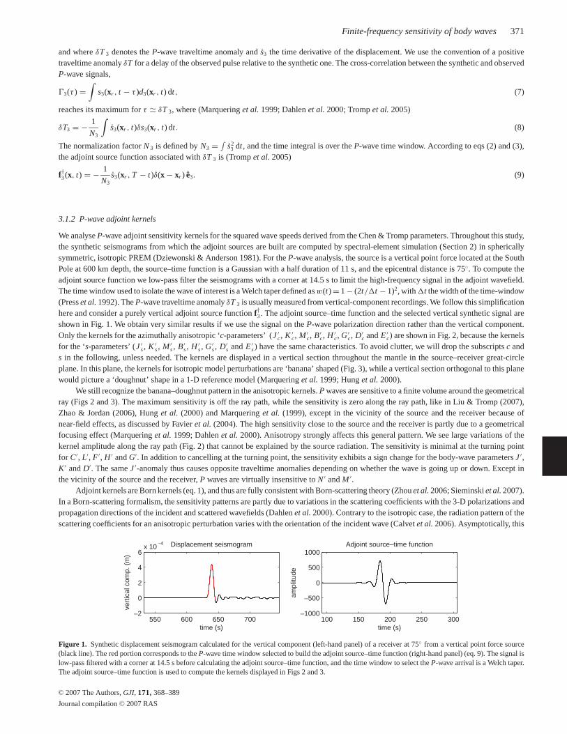
Figure 1. Synthetic displacement seismogram calculated for the vertical component (left-hand panel) of a receiver at 75◦ from a vertical point force source(black line). The red portion corresponds to the P-wave time window selected to build the adjoint source–time function (right-hand panel) (eq. 9). The signal islow-pass filtered with a corner at 14.5 s before calculating the adjoint source–time function, and the time window to select the P-wave arrival is a Welch taper.The adjoint source–time function is used to compute the kernels displayed in Figs 2 and 3.
C© 2007 The Authors, GJI, 171, 368–389
Journal compilation C© 2007 RAS
372 A. Sieminski et al.
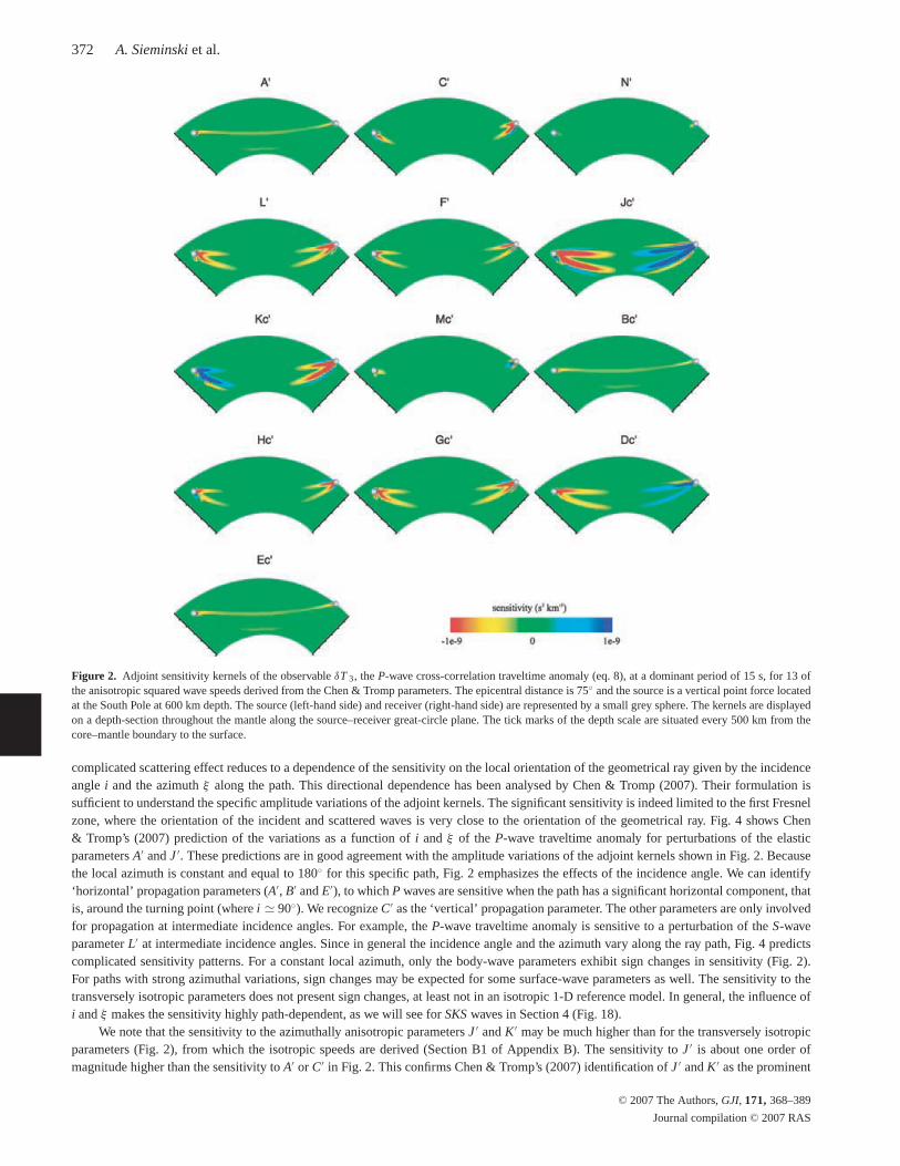
Figure 2. Adjoint sensitivity kernels of the observable δT 3, the P-wave cross-correlation traveltime anomaly (eq. 8), at a dominant period of 15 s, for 13 ofthe anisotropic squared wave speeds derived from the Chen & Tromp parameters. The epicentral distance is 75◦ and the source is a vertical point force locatedat the South Pole at 600 km depth. The source (left-hand side) and receiver (right-hand side) are represented by a small grey sphere. The kernels are displayedon a depth-section throughout the mantle along the source–receiver great-circle plane. The tick marks of the depth scale are situated every 500 km from thecore–mantle boundary to the surface.
complicated scattering effect reduces to a dependence of the sensitivity on the local orientation of the geometrical ray given by the incidenceangle i and the azimuth ξ along the path. This directional dependence has been analysed by Chen & Tromp (2007). Their formulation issufficient to understand the specific amplitude variations of the adjoint kernels. The significant sensitivity is indeed limited to the first Fresnelzone, where the orientation of the incident and scattered waves is very close to the orientation of the geometrical ray. Fig. 4 shows Chen& Tromp’s (2007) prediction of the variations as a function of i and ξ of the P-wave traveltime anomaly for perturbations of the elasticparameters A′ and J ′. These predictions are in good agreement with the amplitude variations of the adjoint kernels shown in Fig. 2. Becausethe local azimuth is constant and equal to 180◦ for this specific path, Fig. 2 emphasizes the effects of the incidence angle. We can identify‘horizontal’ propagation parameters (A′, B′ and E′), to which P waves are sensitive when the path has a significant horizontal component, thatis, around the turning point (where i � 90◦). We recognize C′ as the ‘vertical’ propagation parameter. The other parameters are only involvedfor propagation at intermediate incidence angles. For example, the P-wave traveltime anomaly is sensitive to a perturbation of the S-waveparameter L′ at intermediate incidence angles. Since in general the incidence angle and the azimuth vary along the ray path, Fig. 4 predictscomplicated sensitivity patterns. For a constant local azimuth, only the body-wave parameters exhibit sign changes in sensitivity (Fig. 2).For paths with strong azimuthal variations, sign changes may be expected for some surface-wave parameters as well. The sensitivity to thetransversely isotropic parameters does not present sign changes, at least not in an isotropic 1-D reference model. In general, the influence ofi and ξ makes the sensitivity highly path-dependent, as we will see for SKS waves in Section 4 (Fig. 18).
We note that the sensitivity to the azimuthally anisotropic parameters J ′ and K ′ may be much higher than for the transversely isotropicparameters (Fig. 2), from which the isotropic speeds are derived (Section B1 of Appendix B). The sensitivity to J ′ is about one order ofmagnitude higher than the sensitivity to A′ or C′ in Fig. 2. This confirms Chen & Tromp’s (2007) identification of J ′ and K ′ as the prominent
C© 2007 The Authors, GJI, 171, 368–389
Journal compilation C© 2007 RAS
Finite-frequency sensitivity of body waves 373
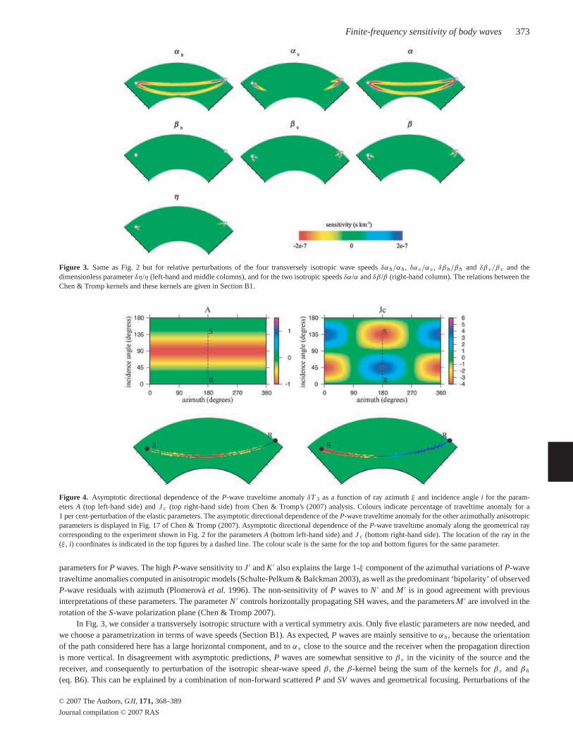
Figure 3. Same as Fig. 2 but for relative perturbations of the four transversely isotropic wave speeds δαh/αh , δαv/αv , δβ h/β h and δβv/βv and thedimensionless parameter δη/η (left-hand and middle columns), and for the two isotropic speeds δα/α and δβ/β (right-hand column). The relations between theChen & Tromp kernels and these kernels are given in Section B1.
Figure 4. Asymptotic directional dependence of the P-wave traveltime anomaly δT 3 as a function of ray azimuth ξ and incidence angle i for the param-eters A (top left-hand side) and J c (top right-hand side) from Chen & Tromp’s (2007) analysis. Colours indicate percentage of traveltime anomaly for a1 per cent-perturbation of the elastic parameters. The asymptotic directional dependence of the P-wave traveltime anomaly for the other azimuthally anisotropicparameters is displayed in Fig. 17 of Chen & Tromp (2007). Asymptotic directional dependence of the P-wave traveltime anomaly along the geometrical raycorresponding to the experiment shown in Fig. 2 for the parameters A (bottom left-hand side) and J c (bottom right-hand side). The location of the ray in the(ξ , i) coordinates is indicated in the top figures by a dashed line. The colour scale is the same for the top and bottom figures for the same parameter.
parameters for P waves. The high P-wave sensitivity to J ′ and K ′ also explains the large 1-ξ component of the azimuthal variations of P-wavetraveltime anomalies computed in anisotropic models (Schulte-Pelkum & Balckman 2003), as well as the predominant ‘bipolarity’ of observedP-wave residuals with azimuth (Plomerova et al. 1996). The non-sensitivity of P waves to N ′ and M ′ is in good agreement with previousinterpretations of these parameters. The parameter N ′ controls horizontally propagating SH waves, and the parameters M ′ are involved in therotation of the S-wave polarization plane (Chen & Tromp 2007).
In Fig. 3, we consider a transversely isotropic structure with a vertical symmetry axis. Only five elastic parameters are now needed, andwe choose a parametrization in terms of wave speeds (Section B1). As expected, P waves are mainly sensitive to αh , because the orientationof the path considered here has a large horizontal component, and to αv close to the source and the receiver when the propagation directionis more vertical. In disagreement with asymptotic predictions, P waves are somewhat sensitive to βv in the vicinity of the source and thereceiver, and consequently to perturbation of the isotropic shear-wave speed β, the β-kernel being the sum of the kernels for βv and β h
(eq. B6). This can be explained by a combination of non-forward scattered P and SV waves and geometrical focusing. Perturbations of the
C© 2007 The Authors, GJI, 171, 368–389
Journal compilation C© 2007 RAS
374 A. Sieminski et al.
isotropic shear-wave speed β do not cause forward scattering for P waves but they do produce P-to-P, SV -to-P and P-to-SV scattering in theplane of the ray path (Dahlen et al. 2000). These scattered waves are weak compared to the scattering effect of perturbations of the isotropicP-wave speed α. However, because of geometrical focusing, they can significantly influence the sensitivity in the vicinity of the source andthe receiver. Apart from this, P-wave sensitivity is well explained by P-to-P near-forward scattering.
A dominant period of 15 s is relatively long for body-wave data. Analysis of the dependence of the sensitivity on wave period showsthat the width of the finite-frequency kernels scales linearly with the square root of the wavelength (e.g. Hung et al. 2000). When theperiod decreases, the kernels will accordingly become narrower, while their overall amplitude will increase, as shown in, for example, Liu& Tromp (2007), Favier & Chevrot (2003) and Marquering et al. (1999). At shorter periods, the anisotropic kernels will however retainthe characteristics discussed above, because the directional dependence does not depend on the period (Dahlen et al. 2000; Calvet et al.2006).
3.2 S waves
3.2.1 S-wave observables and adjoint source definition
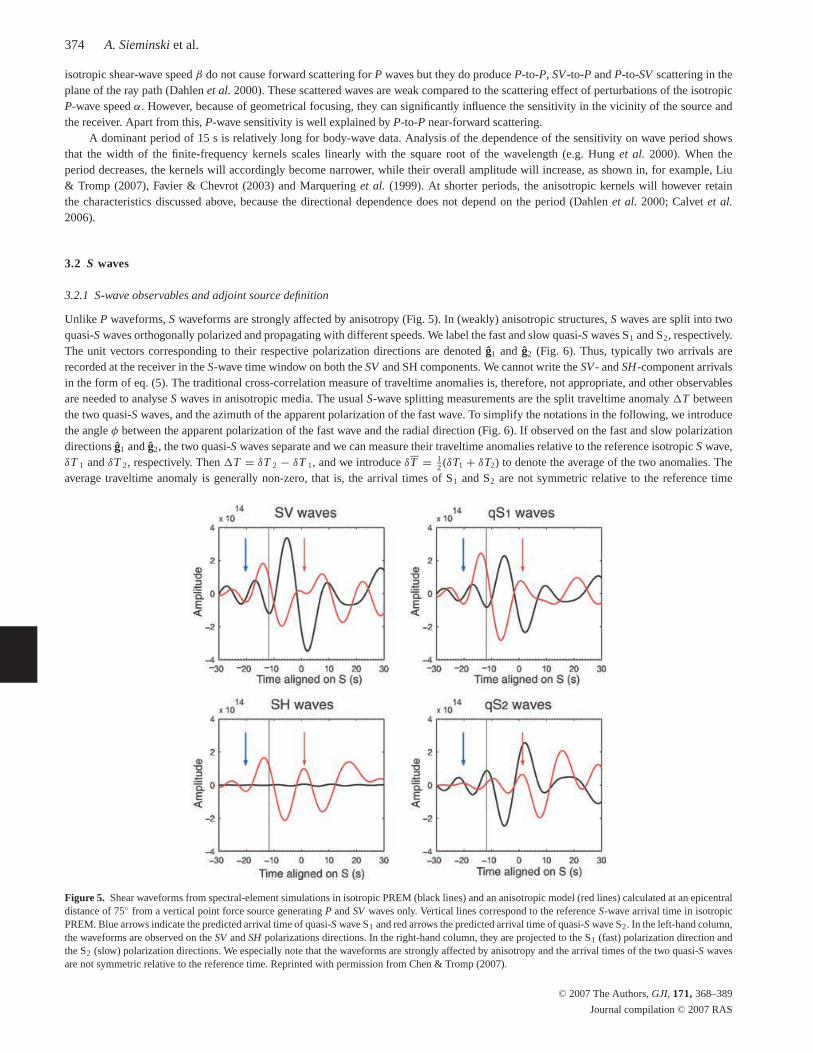
Unlike P waveforms, S waveforms are strongly affected by anisotropy (Fig. 5). In (weakly) anisotropic structures, S waves are split into twoquasi-S waves orthogonally polarized and propagating with different speeds. We label the fast and slow quasi-S waves S1 and S2, respectively.The unit vectors corresponding to their respective polarization directions are denoted g1 and g2 (Fig. 6). Thus, typically two arrivals arerecorded at the receiver in the S-wave time window on both the SV and SH components. We cannot write the SV - and SH-component arrivalsin the form of eq. (5). The traditional cross-correlation measure of traveltime anomalies is, therefore, not appropriate, and other observablesare needed to analyse S waves in anisotropic media. The usual S-wave splitting measurements are the split traveltime anomaly �T betweenthe two quasi-S waves, and the azimuth of the apparent polarization of the fast wave. To simplify the notations in the following, we introducethe angle φ between the apparent polarization of the fast wave and the radial direction (Fig. 6). If observed on the fast and slow polarizationdirections g1 and g2, the two quasi-S waves separate and we can measure their traveltime anomalies relative to the reference isotropic S wave,δT 1 and δT 2, respectively. Then �T = δT 2 − δT 1, and we introduce δT = 1
2 (δT1 + δT2) to denote the average of the two anomalies. Theaverage traveltime anomaly is generally non-zero, that is, the arrival times of S1 and S2 are not symmetric relative to the reference time
Figure 5. Shear waveforms from spectral-element simulations in isotropic PREM (black lines) and an anisotropic model (red lines) calculated at an epicentraldistance of 75◦ from a vertical point force source generating P and SV waves only. Vertical lines correspond to the reference S-wave arrival time in isotropicPREM. Blue arrows indicate the predicted arrival time of quasi-S wave S1 and red arrows the predicted arrival time of quasi-S wave S2. In the left-hand column,the waveforms are observed on the SV and SH polarizations directions. In the right-hand column, they are projected to the S1 (fast) polarization direction andthe S2 (slow) polarization directions. We especially note that the waveforms are strongly affected by anisotropy and the arrival times of the two quasi-S wavesare not symmetric relative to the reference time. Reprinted with permission from Chen & Tromp (2007).
C© 2007 The Authors, GJI, 171, 368–389
Journal compilation C© 2007 RAS
Finite-frequency sensitivity of body waves 375
e1 (SV)
e2 (SH)
^
^
e3 (P)^
g1 (S1)^
g2 (S2)^
(S)
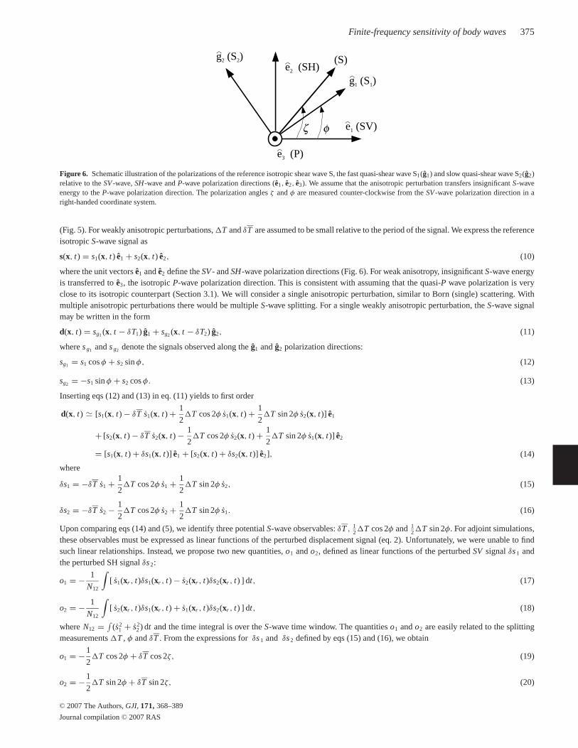
Figure 6. Schematic illustration of the polarizations of the reference isotropic shear wave S, the fast quasi-shear wave S1(g1) and slow quasi-shear wave S2(g2)relative to the SV -wave, SH-wave and P-wave polarization directions (e1, e2, e3). We assume that the anisotropic perturbation transfers insignificant S-waveenergy to the P-wave polarization direction. The polarization angles ζ and φ are measured counter-clockwise from the SV -wave polarization direction in aright-handed coordinate system.
(Fig. 5). For weakly anisotropic perturbations, �T and δT are assumed to be small relative to the period of the signal. We express the referenceisotropic S-wave signal as
s(x, t) = s1(x, t) e1 + s2(x, t) e2, (10)
where the unit vectors e1 and e2 define the SV - and SH-wave polarization directions (Fig. 6). For weak anisotropy, insignificant S-wave energyis transferred to e3, the isotropic P-wave polarization direction. This is consistent with assuming that the quasi-P wave polarization is veryclose to its isotropic counterpart (Section 3.1). We will consider a single anisotropic perturbation, similar to Born (single) scattering. Withmultiple anisotropic perturbations there would be multiple S-wave splitting. For a single weakly anisotropic perturbation, the S-wave signalmay be written in the form
d(x, t) = sg1 (x, t − δT1) g1 + sg2 (x, t − δT2) g2, (11)
where s g1 and s g2 denote the signals observed along the g1 and g2 polarization directions:
sg1 = s1 cos φ + s2 sin φ, (12)
sg2 = −s1 sin φ + s2 cos φ. (13)
Inserting eqs (12) and (13) in eq. (11) yields to first order
d(x, t) � [s1(x, t) − δT s1(x, t) + 1
2�T cos 2φ s1(x, t) + 1
2�T sin 2φ s2(x, t)] e1
+ [s2(x, t) − δT s2(x, t) − 1
2�T cos 2φ s2(x, t) + 1
2�T sin 2φ s1(x, t)] e2
= [s1(x, t) + δs1(x, t)] e1 + [s2(x, t) + δs2(x, t)] e2], (14)
where
δs1 = −δT s1 + 1
2�T cos 2φ s1 + 1
2�T sin 2φ s2, (15)
δs2 = −δT s2 − 1
2�T cos 2φ s2 + 1
2�T sin 2φ s1. (16)
Upon comparing eqs (14) and (5), we identify three potential S-wave observables: δT , 12 �T cos 2φ and 1
2 �T sin 2φ. For adjoint simulations,these observables must be expressed as linear functions of the perturbed displacement signal (eq. 2). Unfortunately, we were unable to findsuch linear relationships. Instead, we propose two new quantities, o1 and o2, defined as linear functions of the perturbed SV signal δs 1 andthe perturbed SH signal δs 2:
o1 = − 1
N12
∫[ s1(xr , t)δs1(xr , t) − s2(xr , t)δs2(xr , t) ] dt, (17)
o2 = − 1
N12
∫[ s2(xr , t)δs1(xr , t) + s1(xr , t)δs2(xr , t) ] dt, (18)
where N12 = ∫(s2
1 + s22 ) dt and the time integral is over the S-wave time window. The quantities o1 and o2 are easily related to the splitting
measurements �T , φ and δT . From the expressions for δs 1 and δs 2 defined by eqs (15) and (16), we obtain
o1 = −1
2�T cos 2φ + δT cos 2ζ, (19)
o2 = −1
2�T sin 2φ + δT sin 2ζ, (20)
C© 2007 The Authors, GJI, 171, 368–389
Journal compilation C© 2007 RAS
376 A. Sieminski et al.
where ζ is the angle between the polarization of the isotropic reference S wave and the radial direction (Fig. 6). In other words, if s(t) denotesthe S isotropic reference waveform, then s 1(t) = s(t) cos ζ and s 2(t) = s(t) sin ζ . The quantities o1 and o2 can be constructed from the splittingmeasurements and the fast polarization direction. We will see in what follows that o1 is a generalization of the traveltime anomaly and o2 ofthe ‘splitting intensity’ first introduced by Chevrot (2000) for SKS splitting.
The observables o1 and o2 have the additional advantage of being related to the two cross-correlations 1(τ ) and 2(τ ) defined by
1(τ ) =∫
s1(xr , t − τ )d1(xr , t) + s2(xr , t + τ )d2(xr , t) dt, (21)
2(τ ) = ∫s1(xr , t − τ )[d2(xr , t) − s2(xr , t) + s1(xr , t)]
+ s2(xr , t − τ )[d1(xr , t) − s1(xr , t) + s2(xr , t)] dt. (22)
The cross-correlations 1(τ ) and 2(τ ) reach their maximum for τ � o1 and τ � o2, respectively. These equations suggest an alternativetechnique to measure the observables o1 and o2 based upon cross-correlation. They confirm these quantities to be temporal observables, sincethey are measured by extracting time information contained in the seismograms.
From eqs (17) and (18) we can readily derive the adjoint source functions f†1 and f†2 associated with the observables o1 and o2,respectively:
f†1 (x, t) = − 1
N12[s1(xr , T − t) e1 − s2(xr , T − t) e2]δ(x − xr ), (23)
f†2 (x, t) = − 1
N12[s2(xr , T − t) e1 + s1(xr , T − t) e2]δ(x − xr ). (24)
For pure SV and SH waves the integral definitions of o1 and o2 and their relationships to the splitting measurements simplify, highlighting thelink with the traditional traveltime anomaly and the splitting intensity. Next, we investigate S-wave sensitivity through these new observablesfor pure SV and SH waves.
3.2.2 SV-wave adjoint kernels
For pure SV waves, the isotropic reference S wave is only observed on the SV -wave polarization direction, that is, s 2(xr , t) = 0 and ζ = 0◦.The integral definitions (17) and (18) of the observables o1 and o2 simplify to
o1 = − 1
N1
∫s1(xr , t)δs1(xr , t) dt, (25)
o2 = − 1
N1
∫s1(xr , t)δs2(xr , t) dt, (26)
with N1 = ∫s2
1 dt . The relationships (19) and (20) between o1 and o2 and the splitting measurements become
o1 = −1
2�T cos 2φ + δT , (27)
o2 = −1
2�T sin 2φ. (28)
In this case, we recognize o2 as the splitting intensity of Chevrot (2000). For vertically transversely isotropic perturbations (i.e. δA′, δC ′,δN ′, δL ′ and δF ′) Chen & Tromp’s (2007) asymptotic formulation predicts that φ = 0◦. Thus, only one S-wave arrival is expected on theSV -component, which leads to o1 = − 1
2 �T + δT = δT1, that is, the SV -wave traveltime anomaly.We compute adjoint sensitivity kernels for the SV -wave observables o1 and o2 for the same source–receiver configuration and parameters
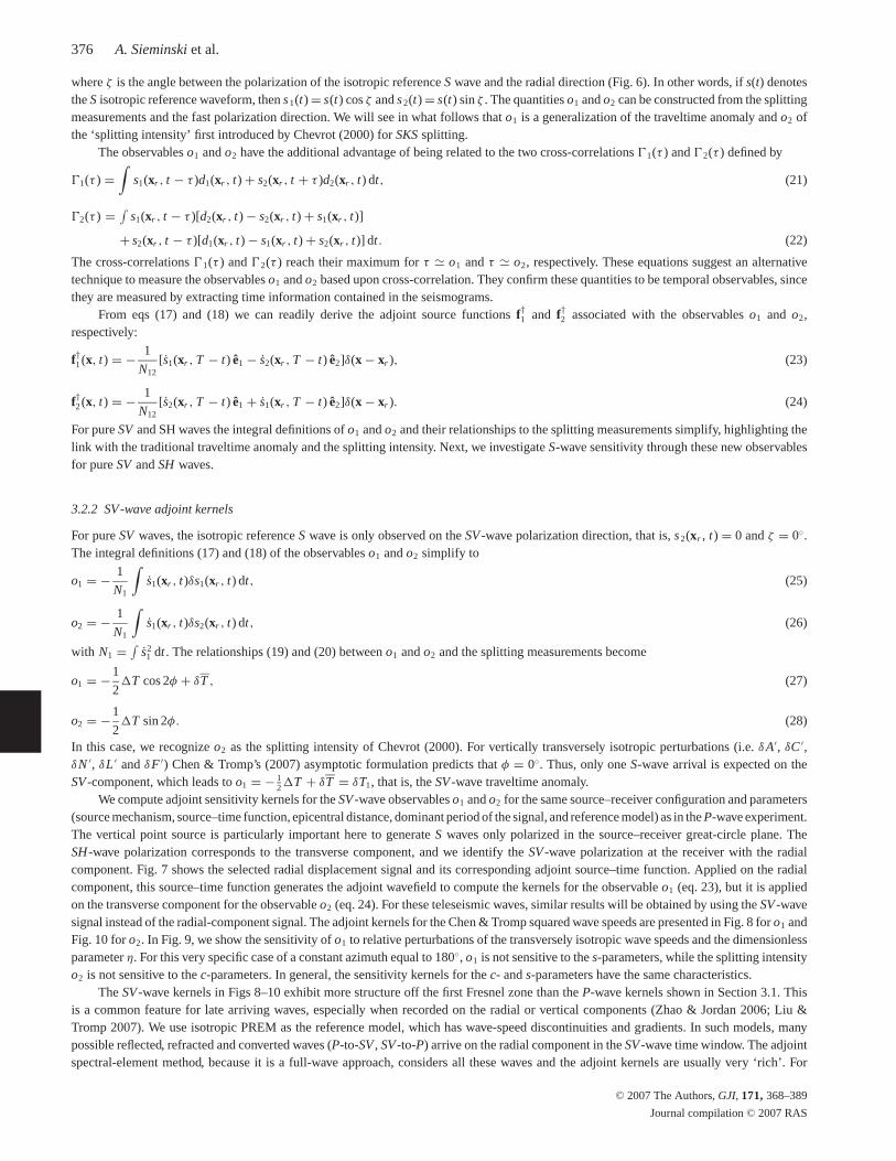
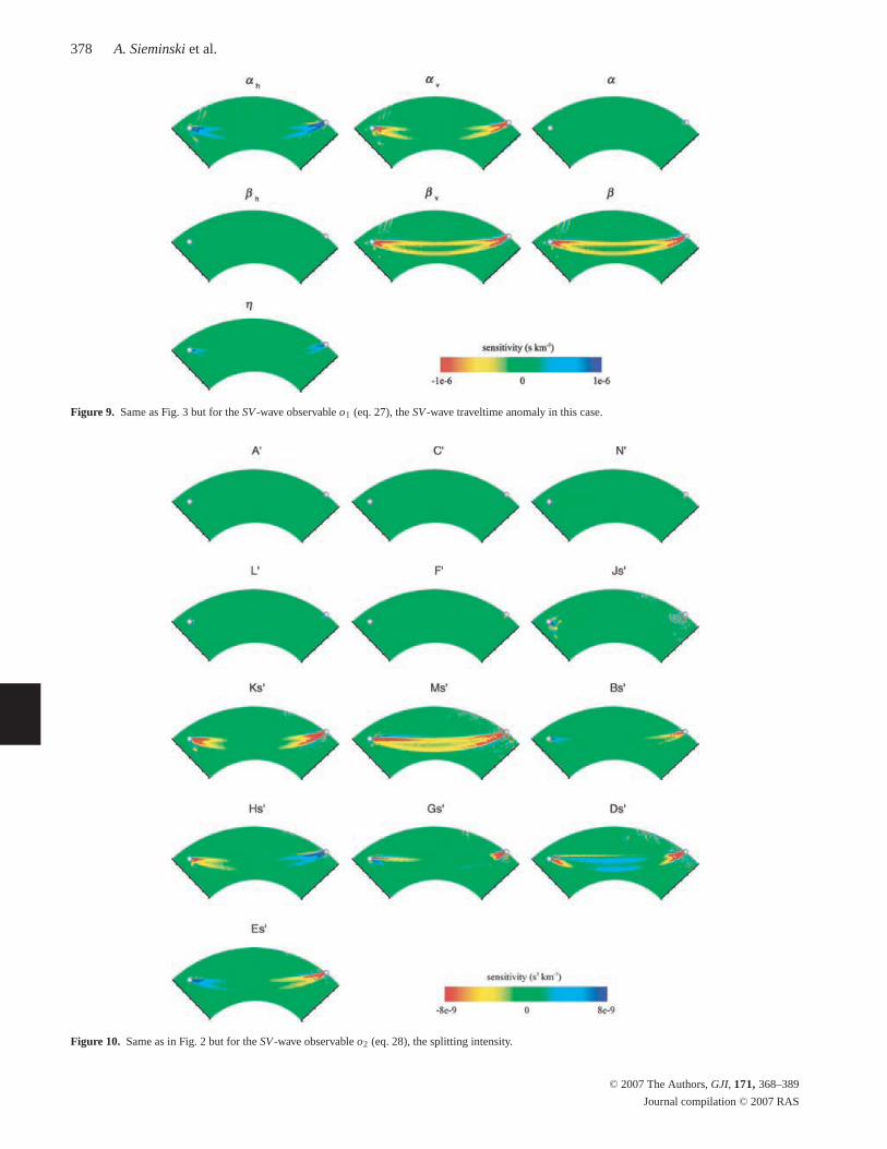
(source mechanism, source–time function, epicentral distance, dominant period of the signal, and reference model) as in the P-wave experiment.The vertical point source is particularly important here to generate S waves only polarized in the source–receiver great-circle plane. TheSH-wave polarization corresponds to the transverse component, and we identify the SV -wave polarization at the receiver with the radialcomponent. Fig. 7 shows the selected radial displacement signal and its corresponding adjoint source–time function. Applied on the radialcomponent, this source–time function generates the adjoint wavefield to compute the kernels for the observable o1 (eq. 23), but it is appliedon the transverse component for the observable o2 (eq. 24). For these teleseismic waves, similar results will be obtained by using the SV -wavesignal instead of the radial-component signal. The adjoint kernels for the Chen & Tromp squared wave speeds are presented in Fig. 8 for o1 andFig. 10 for o2. In Fig. 9, we show the sensitivity of o1 to relative perturbations of the transversely isotropic wave speeds and the dimensionlessparameter η. For this very specific case of a constant azimuth equal to 180◦, o1 is not sensitive to the s-parameters, while the splitting intensityo2 is not sensitive to the c-parameters. In general, the sensitivity kernels for the c- and s-parameters have the same characteristics.
The SV -wave kernels in Figs 8–10 exhibit more structure off the first Fresnel zone than the P-wave kernels shown in Section 3.1. Thisis a common feature for late arriving waves, especially when recorded on the radial or vertical components (Zhao & Jordan 2006; Liu &Tromp 2007). We use isotropic PREM as the reference model, which has wave-speed discontinuities and gradients. In such models, manypossible reflected, refracted and converted waves (P-to-SV , SV -to-P) arrive on the radial component in the SV -wave time window. The adjointspectral-element method, because it is a full-wave approach, considers all these waves and the adjoint kernels are usually very ‘rich’. For
C© 2007 The Authors, GJI, 171, 368–389
Journal compilation C© 2007 RAS
Finite-frequency sensitivity of body waves 377
1100 1150 1200 1250–5
0
5
10x 10
–4
time (s)ra
dial
com
p. (
m)
Displacement seismogram
50 100 150 200 250–500
0
500
time (s)
ampl
itude
Adjoint source–time function
Figure 7. Synthetic displacement seismogram calculated for the radial component (left-hand panel) of a receiver at 75◦ from a vertical point force source(black line). The red portion corresponds to the S-wave time window selected to build the adjoint source–time function (right-hand panel) associated withthe observables o1 and o2 (eqs 17 and 18). The signal is low-pass filtered with a corner at 14.5 s before calculating the adjoint source–time function.The adjoint source–time function is applied to the radial component to compute the kernels for o1 (Figs 8 and 9) and to the transverse component for o2
(Fig. 10).
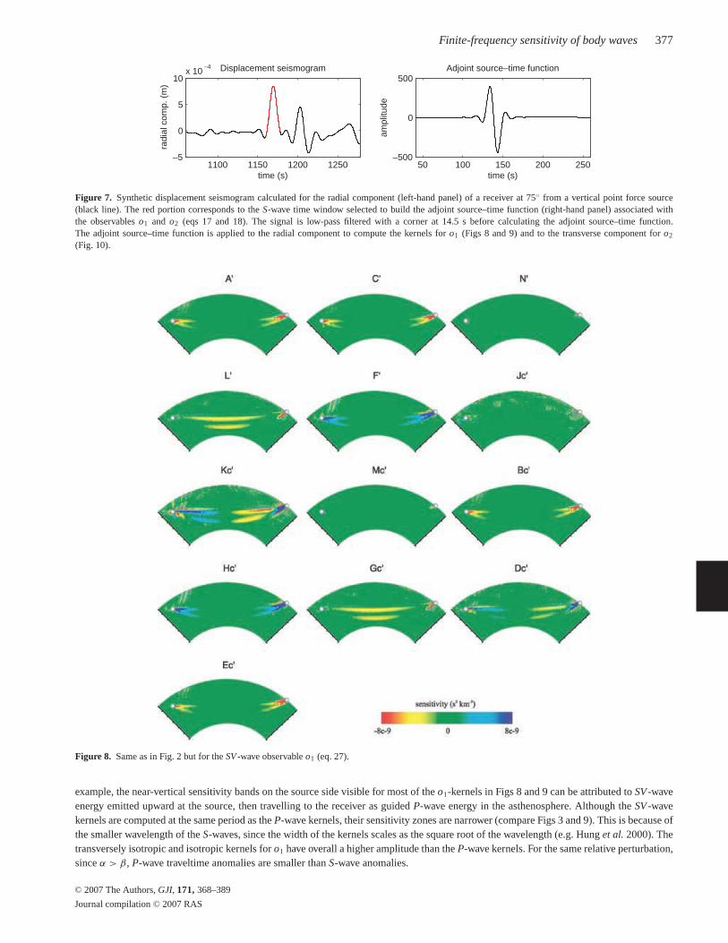
Figure 8. Same as in Fig. 2 but for the SV -wave observable o1 (eq. 27).
example, the near-vertical sensitivity bands on the source side visible for most of the o1-kernels in Figs 8 and 9 can be attributed to SV -waveenergy emitted upward at the source, then travelling to the receiver as guided P-wave energy in the asthenosphere. Although the SV -wavekernels are computed at the same period as the P-wave kernels, their sensitivity zones are narrower (compare Figs 3 and 9). This is because ofthe smaller wavelength of the S-waves, since the width of the kernels scales as the square root of the wavelength (e.g. Hung et al. 2000). Thetransversely isotropic and isotropic kernels for o1 have overall a higher amplitude than the P-wave kernels. For the same relative perturbation,since α > β, P-wave traveltime anomalies are smaller than S-wave anomalies.
C© 2007 The Authors, GJI, 171, 368–389
Journal compilation C© 2007 RAS
378 A. Sieminski et al.
Figure 9. Same as Fig. 3 but for the SV -wave observable o1 (eq. 27), the SV -wave traveltime anomaly in this case.
Figure 10. Same as in Fig. 2 but for the SV -wave observable o2 (eq. 28), the splitting intensity.
C© 2007 The Authors, GJI, 171, 368–389
Journal compilation C© 2007 RAS
Finite-frequency sensitivity of body waves 379
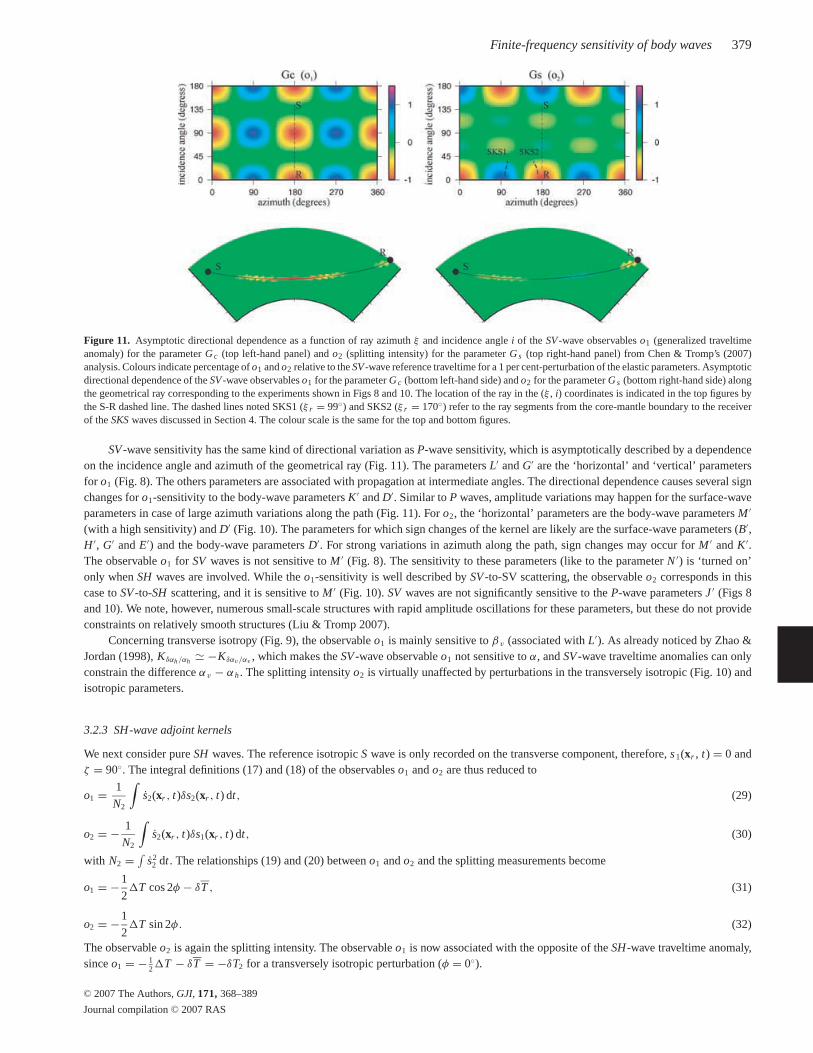
Figure 11. Asymptotic directional dependence as a function of ray azimuth ξ and incidence angle i of the SV -wave observables o1 (generalized traveltimeanomaly) for the parameter G c (top left-hand panel) and o2 (splitting intensity) for the parameter G s (top right-hand panel) from Chen & Tromp’s (2007)analysis. Colours indicate percentage of o1 and o2 relative to the SV -wave reference traveltime for a 1 per cent-perturbation of the elastic parameters. Asymptoticdirectional dependence of the SV -wave observables o1 for the parameter G c (bottom left-hand side) and o2 for the parameter G s (bottom right-hand side) alongthe geometrical ray corresponding to the experiments shown in Figs 8 and 10. The location of the ray in the (ξ , i) coordinates is indicated in the top figures bythe S-R dashed line. The dashed lines noted SKS1 (ξ r = 99◦) and SKS2 (ξ r = 170◦) refer to the ray segments from the core-mantle boundary to the receiverof the SKS waves discussed in Section 4. The colour scale is the same for the top and bottom figures.
SV -wave sensitivity has the same kind of directional variation as P-wave sensitivity, which is asymptotically described by a dependenceon the incidence angle and azimuth of the geometrical ray (Fig. 11). The parameters L′ and G′ are the ‘horizontal’ and ‘vertical’ parametersfor o1 (Fig. 8). The others parameters are associated with propagation at intermediate angles. The directional dependence causes several signchanges for o1-sensitivity to the body-wave parameters K ′ and D′. Similar to P waves, amplitude variations may happen for the surface-waveparameters in case of large azimuth variations along the path (Fig. 11). For o2, the ‘horizontal’ parameters are the body-wave parameters M ′
(with a high sensitivity) and D′ (Fig. 10). The parameters for which sign changes of the kernel are likely are the surface-wave parameters (B′,H ′, G′ and E′) and the body-wave parameters D′. For strong variations in azimuth along the path, sign changes may occur for M ′ and K ′.The observable o1 for SV waves is not sensitive to M ′ (Fig. 8). The sensitivity to these parameters (like to the parameter N ′) is ‘turned on’only when SH waves are involved. While the o1-sensitivity is well described by SV -to-SV scattering, the observable o2 corresponds in thiscase to SV -to-SH scattering, and it is sensitive to M ′ (Fig. 10). SV waves are not significantly sensitive to the P-wave parameters J ′ (Figs 8and 10). We note, however, numerous small-scale structures with rapid amplitude oscillations for these parameters, but these do not provideconstraints on relatively smooth structures (Liu & Tromp 2007).
Concerning transverse isotropy (Fig. 9), the observable o1 is mainly sensitive to βv (associated with L′). As already noticed by Zhao &Jordan (1998), Kδαh/αh � −Kδαv/αv
, which makes the SV -wave observable o1 not sensitive to α, and SV -wave traveltime anomalies can onlyconstrain the difference αv − αh . The splitting intensity o2 is virtually unaffected by perturbations in the transversely isotropic (Fig. 10) andisotropic parameters.
3.2.3 SH-wave adjoint kernels
We next consider pure SH waves. The reference isotropic S wave is only recorded on the transverse component, therefore, s 1(xr , t) = 0 andζ = 90◦. The integral definitions (17) and (18) of the observables o1 and o2 are thus reduced to
o1 = 1
N2
∫s2(xr , t)δs2(xr , t) dt, (29)
o2 = − 1
N2
∫s2(xr , t)δs1(xr , t) dt, (30)
with N2 = ∫s2
2 dt . The relationships (19) and (20) between o1 and o2 and the splitting measurements become
o1 = −1
2�T cos 2φ − δT , (31)
o2 = −1
2�T sin 2φ. (32)
The observable o2 is again the splitting intensity. The observable o1 is now associated with the opposite of the SH-wave traveltime anomaly,since o1 = − 1
2 �T − δT = −δT2 for a transversely isotropic perturbation (φ = 0◦).
C© 2007 The Authors, GJI, 171, 368–389
Journal compilation C© 2007 RAS
380 A. Sieminski et al.
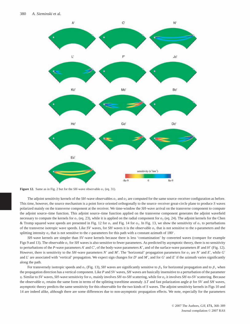
Figure 12. Same as in Fig. 2 but for the SH-wave observable o1 (eq. 31).
The adjoint sensitivity kernels of the SH-wave observables o1 and o2 are computed for the same source–receiver configuration as before.This time, however, the source mechanism is a point force oriented orthogonally to the source–receiver great-circle plane to produce S wavespolarized mainly on the transverse component at the receiver. We time-window the SH-wave arrival on the transverse component to computethe adjoint source–time function. This adjoint source–time function applied on the transverse component generates the adjoint wavefieldnecessary to compute the kernels for o1 (eq. 23), while it is applied on the radial component for o2 (eq. 24). The adjoint kernels for the Chen& Tromp squared wave speeds are presented in Fig. 12 for o1 and Fig. 14 for o2. In Fig. 13, we show the sensitivity of o1 to perturbationsof the transverse isotropic wave speeds. Like SV waves, for SH waves it is the observable o1 that is not sensitive to the s-parameters and thesplitting intensity o2 that is not sensitive to the c-parameters for this path with a constant azimuth of 180◦.
SH-wave kernels are simpler than SV -wave kernels because there is less ‘contamination’ by converted waves (compare for exampleFigs 9 and 13). The observable o1 for SH waves is also sensitive to fewer parameters. As predicted by asymptotic theory, there is no sensitivityto perturbations of the P-wave parameters A′ and C′, of the body-wave parameters K ′, and of the surface-wave parameters B′ and H ′ (Fig. 12).However, there is sensitivity to the SH-wave parameters N ′ and M ′. The ‘horizontal’ propagation parameters for o1 are N ′ and E′, while G′
and L′ are associated with ‘vertical’ propagation. We expect sign changes for D′ and M ′, and for G′ and E′ if the azimuth varies significantlyalong the path.
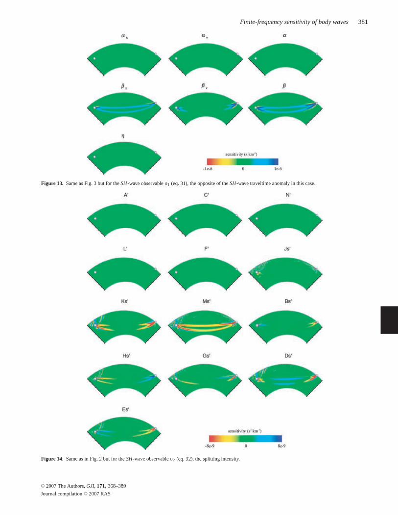
For transversely isotropic speeds and o1 (Fig. 13), SH waves are significantly sensitive to β h for horizontal propagation and to βv whenthe propagation direction has a vertical component. Like P and SV waves, SH waves are basically insensitive to a perturbation of the parameterη. Similar to SV waves, SH-wave sensitivity for o1 mainly involves SH-to-SH scattering, while for o2 it involves SH-to-SV scattering. Becausethe observable o2 retains the same form in terms of the splitting traveltime anomaly �T and fast polarization angle φ for SV and SH waves,asymptotic theory predicts the same sensitivity for this observable for the two kinds of S waves. The adjoint sensitivity kernels in Figs 10 and14 are indeed alike, although there are some differences due to non-asymptotic propagation effects. We note, especially for the parameters
C© 2007 The Authors, GJI, 171, 368–389
Journal compilation C© 2007 RAS
Finite-frequency sensitivity of body waves 381
Figure 13. Same as Fig. 3 but for the SH-wave observable o1 (eq. 31), the opposite of the SH-wave traveltime anomaly in this case.
Figure 14. Same as in Fig. 2 but for the SH-wave observable o2 (eq. 32), the splitting intensity.
C© 2007 The Authors, GJI, 171, 368–389
Journal compilation C© 2007 RAS
382 A. Sieminski et al.
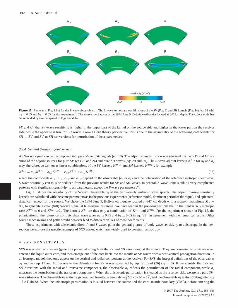
Figure 15. Same as in Fig. 3 but for the S-wave observable o1. The S-wave kernels are combinations of the SV (Fig. 9) and SH kernels (Fig. 14) (eq. 33 witha1 � 0.35 and b1 � 0.65 for this experiment). The source mechanism is the 1994 June 9, Bolivia earthquake located at 647 km depth. The colour scale hasbeen divided by two compared to Figs 9 and 14.
M ′ and G′, that SV -wave sensitivity is higher in the upper part of the kernel on the source side and higher in the lower part on the receiverside, while the opposite is true for SH waves. From a Born theory perspective, this is due to the asymmetry of the scattering coefficients forSH-to-SV and SV -to-SH conversions for perturbation of these parameters.
3.2.4 General S-wave adjoint kernels
An S-wave signal can be decomposed into pure SV and SH signals (eq. 10). The adjoint sources for S waves (derived from eqs 17 and 18) aresums of the adjoint sources for pure SV (eqs 25 and 26) and pure SH waves (eqs 29 and 30). The S-wave adjoint kernels K S1,2 for o1 and o2
may, therefore, be written as linear combinations of the SV kernels K SV1,2 and SH kernels K SH1,2 , for example
K S1,2 = a1,2 K SV1 + b1,2 K SH1 + c1,2 K SV2 + d1,2 K SH2 , (33)
where the coefficients a1,2, b1,2, c1,2 and d 1,2 depend on the observable (o1 or o2) and the polarization of the reference isotropic shear wave.S-wave sensitivity can thus be deduced from the previous results for SV and SH waves. In general, S-wave kernels exhibit very complicatedpatterns with significant sensitivity to all parameters, except the P-wave parameters J ′.
Fig. 15 shows the sensitivity of the S-wave observable o1 to the transversely isotropic wave speeds. The adjoint S-wave sensitivitykernels are calculated with the same parameters as in the previous experiments (reference model, dominant period of the signal, and epicentraldistance), except for the source. We chose the 1994 June 9, Bolivia earthquake located at 647 km depth with a moment magnitude M w =8.2, to generate a clear (full) S-wave signal at teleseismic distances. We have seen in the previous sections that in the transversely isotropiccase K SV2 � 0 and K SH2 �0 . The kernels K S1 are thus only a combination of K SV1 and K SH1 . For the experiment shown in Fig. 15, thepolarization of the reference isotropic shear wave gives a1 � 0.35 and b1 � 0.65 in eq. (33), in agreement with the numerical results. Othersource mechanisms and paths would however lead to different values of these coefficients.
These experiments with teleseismic direct P and S waves paint the general picture of body-wave sensitivity to anisotropy. In the nextsection we explore the specific example of SKS waves, which are widely used to constrain anisotropy.
4 S K S S E N S I T I V I T Y
SKS waves start as S waves (generally polarized along both the SV and SH directions) at the source. They are converted to P waves whenentering the liquid outer core, and then emerge out of the core back into the mantle as SV waves with a near-vertical propagation direction. Inan isotropic model, they only appear on the vertical and radial components at the receiver. For SKS, the integral definitions of the observableso1 and o2 (eqs 17 and 18) reduce to the definitions for SV waves governed by eqs (25) and (26) (s 2 = 0). If we identify the SV - andSH-directions with the radial and transverse components, the observable o1 reflects the perturbation of the radial component, while o2
measures the perturbation of the transverse component. When the anisotropic perturbation is situated on the receiver side, we are in a pure SV -wave situation. The observable o1 is then a generalized traveltime anomaly − 1
2 �T cos 2φ + δT , and the observable o2 is the splitting intensity− 1
2 �T sin 2φ. When the anisotropic perturbation is located between the source and the core–mantle boundary (CMB), before entering the
C© 2007 The Authors, GJI, 171, 368–389
Journal compilation C© 2007 RAS
Finite-frequency sensitivity of body waves 383
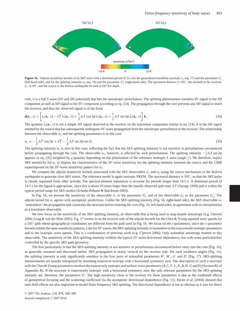
Figure 16. Adjoint sensitivity kernels of an SKS wave with a dominant period of 15 s for the generalized traveltime anomaly o1 (eq. 17) and the parameter G ′c
(left-hand side), and for the splitting intensity o2 (eq. 18) and the parameter G ′s (right-hand side). The epicentral distance is 105◦, the azimuth at the receiver,
ξ r , is 99◦, and the source is the Bolivia earthquake located at 647 km depth.
core, it is a full S wave (SV and SH polarized) that hits the anisotropic perturbation. The splitting phenomenon transfers SV signal to the SHcomponent as well as SH signal to the SV component according to eq. (14). The propagation through the core prevents any SH signal to reachthe receiver, and thus the observed signal is of the form
d(xr , t) �[
s1(xr , t) − δT s1(xr , t) + 1
2�T cos 2φ s1(xr , t) + 1
2�T sin 2φ ˙s2(xr , t)
]e1. (34)
The quantity s2(xr , t) is not a simple SH signal observed at the receiver on the transverse component similar to eq. (14). It is the SH signalemitted by the source that has subsequently undergone SV -wave propagation from the anisotropic perturbation to the receiver. The relationshipbetween the observable o1 and the splitting parameters is in this case
o1 = −1
2�T cos 2φ + δT − 1
4�T sin 2φ sin 2ζ. (35)
The splitting intensity o2 is zero in this case, reflecting the fact that the SKS-splitting intensity is not sensitive to perturbations encounteredbefore propagating through the core. The observable o1, however, is affected by such perturbations. The splitting intensity − 1
2 �T sin 2φ
appears in eq. (35) weighted by a quantity depending on the polarization of the reference isotropic S wave (angle ζ ). We therefore, expectSKS sensitivity for o1 to display the characteristics of the SV -wave sensitivity for the splitting intensity between the source and the CMBsuperimposed on the SV -wave sensitivity pattern for o1.
We compute the adjoint sensitivity kernels associated with the SKS observables o1 and o2 using the source mechanism of the Boliviaearthquake to generate clear SKS waves. The reference model is again isotropic PREM. The epicentral distance is 105◦, so that the SKS pulseis clearly separated from other arrivals. The spectral-element simulation is accurate for periods longer than 14.5 s. A dominant period of14.5 s for the signal is appropriate, since this is about 10 times larger than the usually observed split time �T (Savage 1999) and is within thetypical period range for SKS studies (Schulte-Pelkum & Balckman 2003).
In Fig. 16, we present the sensitivity of the observable o1 to the parameter G ′c and of the observable o2 to the parameter G ′
s . Theadjoint kernel for o1 agrees with asymptotic predictions. Unlike the SKS-splitting intensity (Fig. 16, right-hand side), the SKS observable o1
‘remembers’ the propagation and constrains the structure before entering the core (Fig. 16, left-hand side), in agreement with its interpretationas a traveltime observable.
We now focus on the sensitivity of the SKS-splitting intensity, an observable that is being used to map mantle anisotropy (e.g. Chevrot2006; Long & van der Hilst 2005). Fig. 17 zooms in on the receiver side of the adjoint kernels for the Chen & Tromp squared wave speeds fora 105◦ path whose geographical coordinates are different from the path used in Fig. 16. We focus on the s-parameters, since the c-parameterkernels exhibit the same sensitivity patterns. Like for SV waves, the SKS-splitting intensity is insensitive to the transversely isotropic parametersand to the isotropic wave speeds. This is a confirmation of previous work (e.g. Chevrot 2006). Only azimuthal anisotropy matters to thisobservable. The sensitivity of the SKS-splitting intensity exhibits the typical SV -wave directional dependence, but with some particularitiescontrolled by the specific SKS path-geometry.
The first particularity is that the SKS-splitting intensity is not sensitive to perturbations encountered before entry into the core (Fig. 16),as generally assumed and discussed earlier. SKS propagation is nearly vertical on the receiver side. For such incidence angles (Fig. 11),the splitting intensity is only significantly sensitive to the four pairs of azimuthal parameters K ′, M ′, G′ and D′ (Fig. 17). SKS-splittingmeasurements are usually interpreted by assuming transverse isotropy with a horizontal symmetry axis. The description of such a structurewith the Chen & Tromp parameters involves the transversely isotropic and surface-wave parameters (A, C, F, L, N , B, H , G and E) (Section B2 ofAppendix B). If the structure is transversely isotropic with a horizontal symmetry axis, the only relevant parameters for the SKS-splittingintensity are, therefore, the parameters G′. The high sensitivity close to the receiver for these parameters is due to the combined effectsof geometrical focusing and the scattering coefficient via the asymptotic directional dependence (Fig. 11). Favier et al. (2004) showed thatnear-field effects are also important to model finite-frequency SKS splitting. The directional dependence is not as obvious as it was for direct
C© 2007 The Authors, GJI, 171, 368–389
Journal compilation C© 2007 RAS
384 A. Sieminski et al.
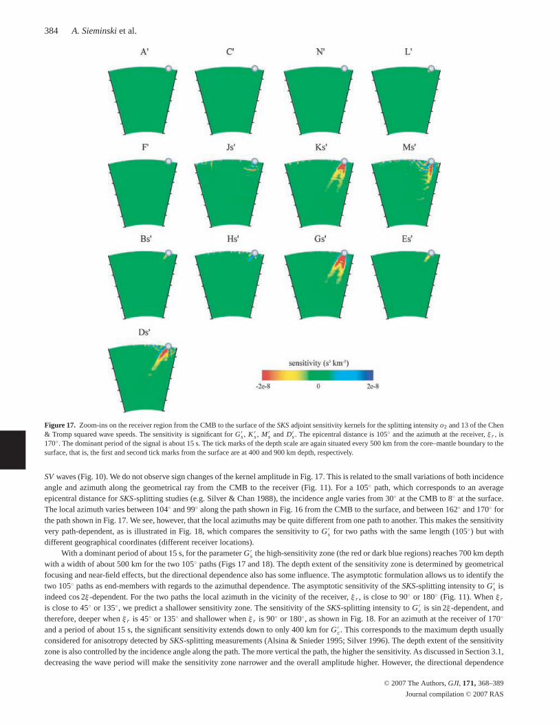
Figure 17. Zoom-ins on the receiver region from the CMB to the surface of the SKS adjoint sensitivity kernels for the splitting intensity o2 and 13 of the Chen& Tromp squared wave speeds. The sensitivity is significant for G ′
s , K ′s , M ′
s and D′s . The epicentral distance is 105◦ and the azimuth at the receiver, ξ r , is
170◦. The dominant period of the signal is about 15 s. The tick marks of the depth scale are again situated every 500 km from the core–mantle boundary to thesurface, that is, the first and second tick marks from the surface are at 400 and 900 km depth, respectively.
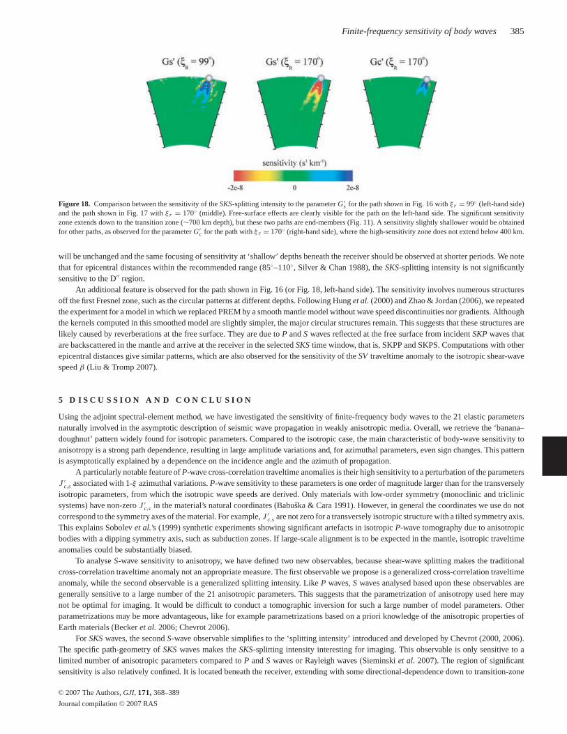
SV waves (Fig. 10). We do not observe sign changes of the kernel amplitude in Fig. 17. This is related to the small variations of both incidenceangle and azimuth along the geometrical ray from the CMB to the receiver (Fig. 11). For a 105◦ path, which corresponds to an averageepicentral distance for SKS-splitting studies (e.g. Silver & Chan 1988), the incidence angle varies from 30◦ at the CMB to 8◦ at the surface.The local azimuth varies between 104◦ and 99◦ along the path shown in Fig. 16 from the CMB to the surface, and between 162◦ and 170◦ forthe path shown in Fig. 17. We see, however, that the local azimuths may be quite different from one path to another. This makes the sensitivityvery path-dependent, as is illustrated in Fig. 18, which compares the sensitivity to G ′
s for two paths with the same length (105◦) but withdifferent geographical coordinates (different receiver locations).
With a dominant period of about 15 s, for the parameter G ′s the high-sensitivity zone (the red or dark blue regions) reaches 700 km depth
with a width of about 500 km for the two 105◦ paths (Figs 17 and 18). The depth extent of the sensitivity zone is determined by geometricalfocusing and near-field effects, but the directional dependence also has some influence. The asymptotic formulation allows us to identify thetwo 105◦ paths as end-members with regards to the azimuthal dependence. The asymptotic sensitivity of the SKS-splitting intensity to G ′
s isindeed cos 2ξ -dependent. For the two paths the local azimuth in the vicinity of the receiver, ξ r , is close to 90◦ or 180◦ (Fig. 11). When ξ r
is close to 45◦ or 135◦, we predict a shallower sensitivity zone. The sensitivity of the SKS-splitting intensity to G ′c is sin 2ξ -dependent, and
therefore, deeper when ξ r is 45◦ or 135◦ and shallower when ξ r is 90◦ or 180◦, as shown in Fig. 18. For an azimuth at the receiver of 170◦
and a period of about 15 s, the significant sensitivity extends down to only 400 km for G ′c. This corresponds to the maximum depth usually
considered for anisotropy detected by SKS-splitting measurements (Alsina & Snieder 1995; Silver 1996). The depth extent of the sensitivityzone is also controlled by the incidence angle along the path. The more vertical the path, the higher the sensitivity. As discussed in Section 3.1,decreasing the wave period will make the sensitivity zone narrower and the overall amplitude higher. However, the directional dependence
C© 2007 The Authors, GJI, 171, 368–389
Journal compilation C© 2007 RAS
Finite-frequency sensitivity of body waves 385
Figure 18. Comparison between the sensitivity of the SKS-splitting intensity to the parameter G ′s for the path shown in Fig. 16 with ξ r = 99◦ (left-hand side)
and the path shown in Fig. 17 with ξ r = 170◦ (middle). Free-surface effects are clearly visible for the path on the left-hand side. The significant sensitivityzone extends down to the transition zone (∼700 km depth), but these two paths are end-members (Fig. 11). A sensitivity slightly shallower would be obtainedfor other paths, as observed for the parameter G ′
c for the path with ξ r = 170◦ (right-hand side), where the high-sensitivity zone does not extend below 400 km.
will be unchanged and the same focusing of sensitivity at ‘shallow’ depths beneath the receiver should be observed at shorter periods. We notethat for epicentral distances within the recommended range (85◦–110◦, Silver & Chan 1988), the SKS-splitting intensity is not significantlysensitive to the D′′ region.
An additional feature is observed for the path shown in Fig. 16 (or Fig. 18, left-hand side). The sensitivity involves numerous structuresoff the first Fresnel zone, such as the circular patterns at different depths. Following Hung et al. (2000) and Zhao & Jordan (2006), we repeatedthe experiment for a model in which we replaced PREM by a smooth mantle model without wave speed discontinuities nor gradients. Althoughthe kernels computed in this smoothed model are slightly simpler, the major circular structures remain. This suggests that these structures arelikely caused by reverberations at the free surface. They are due to P and S waves reflected at the free surface from incident SKP waves thatare backscattered in the mantle and arrive at the receiver in the selected SKS time window, that is, SKPP and SKPS. Computations with otherepicentral distances give similar patterns, which are also observed for the sensitivity of the SV traveltime anomaly to the isotropic shear-wavespeed β (Liu & Tromp 2007).
5 D I S C U S S I O N A N D C O N C L U S I O N
Using the adjoint spectral-element method, we have investigated the sensitivity of finite-frequency body waves to the 21 elastic parametersnaturally involved in the asymptotic description of seismic wave propagation in weakly anisotropic media. Overall, we retrieve the ‘banana–doughnut’ pattern widely found for isotropic parameters. Compared to the isotropic case, the main characteristic of body-wave sensitivity toanisotropy is a strong path dependence, resulting in large amplitude variations and, for azimuthal parameters, even sign changes. This patternis asymptotically explained by a dependence on the incidence angle and the azimuth of propagation.
A particularly notable feature of P-wave cross-correlation traveltime anomalies is their high sensitivity to a perturbation of the parametersJ ′
c,s associated with 1-ξ azimuthal variations. P-wave sensitivity to these parameters is one order of magnitude larger than for the transverselyisotropic parameters, from which the isotropic wave speeds are derived. Only materials with low-order symmetry (monoclinic and triclinicsystems) have non-zero J ′
c,s in the material’s natural coordinates (Babuska & Cara 1991). However, in general the coordinates we use do notcorrespond to the symmetry axes of the material. For example, J ′
c,s are not zero for a transversely isotropic structure with a tilted symmetry axis.This explains Sobolev et al.’s (1999) synthetic experiments showing significant artefacts in isotropic P-wave tomography due to anisotropicbodies with a dipping symmetry axis, such as subduction zones. If large-scale alignment is to be expected in the mantle, isotropic traveltimeanomalies could be substantially biased.
To analyse S-wave sensitivity to anisotropy, we have defined two new observables, because shear-wave splitting makes the traditionalcross-correlation traveltime anomaly not an appropriate measure. The first observable we propose is a generalized cross-correlation traveltimeanomaly, while the second observable is a generalized splitting intensity. Like P waves, S waves analysed based upon these observables aregenerally sensitive to a large number of the 21 anisotropic parameters. This suggests that the parametrization of anisotropy used here maynot be optimal for imaging. It would be difficult to conduct a tomographic inversion for such a large number of model parameters. Otherparametrizations may be more advantageous, like for example parametrizations based on a priori knowledge of the anisotropic properties ofEarth materials (Becker et al. 2006; Chevrot 2006).
For SKS waves, the second S-wave observable simplifies to the ‘splitting intensity’ introduced and developed by Chevrot (2000, 2006).The specific path-geometry of SKS waves makes the SKS-splitting intensity interesting for imaging. This observable is only sensitive to alimited number of anisotropic parameters compared to P and S waves or Rayleigh waves (Sieminski et al. 2007). The region of significantsensitivity is also relatively confined. It is located beneath the receiver, extending with some directional-dependence down to transition-zone
C© 2007 The Authors, GJI, 171, 368–389
Journal compilation C© 2007 RAS
386 A. Sieminski et al.
depths. It is quite different from the surface-wave sensitivity zone (Sieminski et al. 2007), explaining the usual poor correlation betweensurface-wave and SKS-splitting studies (Montagner et al. 2000). Because SKS splitting samples the mantle deeper than fundamental-modesurface waves at intermediate periods, it seems interesting to combine surface-wave data and SKS-splitting measurements to better constrainthe anisotropic structure of the transition zone, for example. Measurements of the splitting intensity for teleseismic S waves are sometimesused to complement SKS-data sets (e.g. Savage 1999; Long & van der Hilst 2005). We cannot compute adjoint sensitivity kernels for theS-wave splitting intensity. However, from the analysis of the S-wave generalized splitting intensity, we expect S-wave splitting intensity to besensitive to structure all along the ray path. This may bias the results when using S-wave splitting to constrain anisotropy beneath the receiver.
The sensitivity of the SKS-splitting intensity has previously been described by the formulation of Favier & Chevrot (2003) and Favieret al. (2004). They applied Born-scattering theory with a plane-wave description and focused on the sensitivity to two perturbation parameters.These parameters are directly related to the parameters we used in this study (Section B2), so that the results can be compared. Working withplane waves misses the effects of variations of the incidence angle and azimuth along the path that partly control the sensitivity pattern (i.e. thedepth extent of the significant sensitivity zone), and it is also difficult to model free-surface effects. It is not clear yet whether these limitationsare significant for imaging. A full-wave approach, such as the adjoint spectral-element method, naturally models all these effects, as well asthe near field, which makes the technique, therefore, very promising for significant progress in anisotropic imaging.
A C K N O W L E D G M E N T S
We thank Sonja Greve, Martha Savage, an anonymous reviewer and editor Cindy Ebinger for helpful comments and suggestions. The adjointspectral-element computations discussed in this paper were performed on Caltech’s Division of Geological & Planetary Sciences Dell cluster.The source code for the adjoint spectral-element simulations is freely available from www.geodynamics.org . We gratefully acknowledgesupport from the European Commission’s Human Resources and Mobility Programme, Marie Curie Research Training Networks, FP6 and bythe National Science Foundation under grant EAR-0309576. This is contribution no 9170 of the Division of Geological & Planetary Sciencesof the Californian Institute of Technology.
R E F E R E N C E S
Alsina, D. & Snieder, R., 1995. Small-scale sublithospheric continental man-tle deformation: constraints from SKS splitting observations, Geophys. J.Int., 123, 431–448.
Babuska, V. & Cara, M., 1991. Seismic Anisotropy in the Earth, KluwerAcademic, Dordrecht.
Becker, T.W., Chevrot, S., Schulte-Pelkum, V. & Blackman, D.K., 2006.Statistical properties of seismic anisotropy predicted by upper man-tle geodynamic models, J. geophys. Res., 111, B08309, doi:10.1029/2005JB004095.
Calvet, M., Chevrot, S. & Souriau, A., 2006. P-wave propagation in trans-versely isotropic media I. Finite-frequency theory, Phys. Earth planet.Int., 156, 12–20.
Chen, M. & Tromp, J., 2007. Theoretical and numerical investigation ofglobal and regional seismic wave propagation in weakly anisotropic Earthmodels, Geophys. J. Int., 168, 1130–1152.
Chevrot, S., 2000. Multichannel analysis of shear wave splitting, J. geophys.Res., 105, 21 579–21 590.
Chevrot, S., 2006. Finite-frequency vectorial tomography: a new methodfor high resolution imaging of mantle anisotropy, Geophys. J. Int., 165,641–657.
Dahlen, F.A., Hung, S.-H. & Nolet, G., 2000. Frechet kernels for finite-frequency traveltimes-I. Theory, Geophys. J. Int., 141, 157–174.
Dziewonski, A.M. & Anderson, D.L., 1981. Preliminary Reference EarthModel, Phys. Earth planet. Inter., 25, 297–356.
Farra, V., 2001. High-order perturbations of the phase velocity and polar-ization of qP and qS waves in anisotropic media, Geophys. J. Int., 147,93–104.
Favier, N. & Chevrot, S., 2003. Sensitivity kernels for shear wave splittingin transverse isotropic media, Geophys. J. Int., 153, 213–228.
Favier, N., Chevrot, S. & Komatitsch, D., 2004. Near-field influence onshear wave splitting and traveltime sensitivity kernels, Geophys. J. Int.,156, 467–482.
Gresillaud, A. & Cara, M., 1996. Anisotropy and P-wave tomography: anew approach for inverting teleseismic data from a dense array of sta-tions, Geophys. J. Int., 126, 77–91.
Hess, H.H., 1964. Seismic anisotropy of the uppermost mantle under oceans,Nature, 203, 629–631.
Hung, S.-H., Dahlen, F.A. & Nolet, G., 2000. Frechet kernels for finite-frequency traveltimes-II. Examples, Geophys. J. Int., 141, 175–203.
Jech, J. & Psencık, I., 1989. First-order perturbation method for anisotropicmedia, Geophys. J. Int., 99, 369–376.
Kaminski, E. &Ribe, N.L.M., 2002. Timescales for the evolution of seis-mic anisotropy in mantle flow, Geochem. Geophys. Geosyst., 3(1),10.1029/2001GC000222.
Komatitsch, D. & Vilotte, J.P., 1998. The spectral-element method: an effi-cient tool to simulate the seismic reponse of 2D and 3D geological struc-tures, Bull. seism. Soc. Am., 88(2), 368–392.
Komatitsch, D. & Tromp, J., 2002a. Spectral-element simulations of globalseismic wave propagation-I. Validation, Geophys. J. Int., 149, 390–412.
Komatitsch, D. & Tromp, J., 2002b. Spectral-element simulations of globalseismic wave propagation-II. Three-dimensional models, oceans, rotationand self-gravitation, Geophys. J. Int., 150, 303–318.
Larson, E., Tromp, J. & Ekstrom, G., 1998. Effects of slight anisotropy onsurface waves, Geophys. J. Int., 132, 654–666.
Liu, Q. & Tromp, J., 2006. Finite-frequency kernels based upon adjointmethods, Bull. seism. Soc. Am., 96, 2383–2397.
Liu, Q. & Tromp, J., 2007. Finite-frequency sensitivity kernels for globalseismic wave propagation based upon adjoint methods, Geophys. J. Int.,in preparation.
Long, M.D. & van der Hilst, R.D., 2005. Estimating shear-wave splittingparameters from broadband recordings in Japan: a comparison of threemethods, Bull. seism. Soc. Am., 95, 1346–1358.
Love, A.E.H., 1911. Some Problems of Geodynamics, Cambridge UniversityPress, Cambridge.
Mainprice, D., Barruol, G. & Ben Ismaı l, W., 2000. The seismic anisotropyof the Earth’s mantle: from single crystal to polycrystal, Geophys. Mono-graph, 117, 237–264.
Marquering, H., Dahlen, F.A. & Nolet, G., 1999. Three-dimensional sensitiv-ity kernels for finie-frequency traveltimes: the banana-doughnut paradox,Geophys. J. Int., 137, 805–815.
Montagner, J.P. & Nataf, H.C., 1986. A simple method for inverting theazimuthal anisotropy of surface waves, J. geophys. Res., 91, 511–520.
Montagner, J.P., Griot-Pommera, D.A. & Lave, J., 2000. How to relate bodywave and surface wave anisotropy?, J. geophys. Res., 105, 19 015–19 027.
Plomerova, J., Sıleny, J. & Babuska, V., 1996. Joint interpretation of upper-mantle anisotropy based on teleseismic P-travel time delays and inversion
C© 2007 The Authors, GJI, 171, 368–389
Journal compilation C© 2007 RAS
Finite-frequency sensitivity of body waves 387
of shear-wave splitting parameters, Phys. Earth. planet. Int., 95, 293–309.
Press, W., Teukolsky, S., Vetterling, W. & Flannery, B., 1992. NumericalRecipes in FORTRAN: The Art of Scientific Computing, Cambridge Uni-verstity Press, Cambridge.
Savage, M.K., 1999. Seismic anisotropy and mantle deformation: whathave we learned from shear wave splitting?, Rev. Geophys., 37, 65–106.
Schulte-Pelkum, V. & Balckman, D.K., 2003. A synthesis of seismic P andS anisotropy, Geophys. J. Int., 154, 166–178.
Silver, P.G., 1996. Seismic anisotropy beneath the continents: Probing thedepths of geology, Annu. Rev. Earth Planet. Sci., 24, 385–432.
Silver, P.G. & Chan, W.W., 1988. Implications for continental structure andevolution from seismic anisotropy, Nature, 335, 34–39.
Sieminski, A., Liu, Q., Trampert, J. & Tromp, J., 2007. Finite-frequencysensitivity of surface waves to anisotropy based upon adjoint methods,Geophys. J. Int., 168, 1153–1174.
Smith, M.L. & Dahlen, F.A., 1973. The azimuthal dependence of Love andRayleigh wave propagation in a slightly anisotropic medium, J. geophys.Res., 78, 3321–3333.
Sobolev, S.V., Gresillaud, A. & Cara, M., 1999. How robust is isotropicdelay time tomography for anisotropic mantle?, Geophys. Res. Lett., 26,509–512.
Tape, C., Liu, Q. & Tromp, J., 2007. Finite frequency tomography usingadjoint methods—methodology and examples using membrane surfacewaves, Geophys. J. Int., 168, 1105–1129.
Tarantola, A., 1984. Inversion of seismic reflection data in acoustic approx-imation, Geophysics, 49, 1259–1266.
Tarantola, A., 1987. Inversion of travel times and seismic waveforms, inSeismic Tomography, pp. 135–157, ed. Nolet G., Reidel, Dordrecht.
Tarantola, A., 1988. Theoretical background for the inversion of seismicwaveforms, including elasticity and attenuation, Pure appl. Geophys., 128,365–399.
Tromp, J., Tape, C. & Liu, Q., 2005. Seismic tomography, adjoint meth-ods, time reversal and banana-doughnut kernels, Geophys. J. Int., 160,195–216.
Vinnik, L.P., Farra, V. & Romanowicz, B., 1989. Azimuthal anisotropy inthe Earth from observations of SKS at Geoscope and NARS broadbandstations, Bull. seism. Soc. Am., 79, 1542–1558.
Wessel, P. & Smith, W.H.F., 1995. New version of the Generic MappingTools released, EOS Trans. Am. geophys. Un., 76, 329.
Zhao, L. & Jordan, T.H., 1998. Sensitivity of frequency-dependent travel-times to laterally heterogenous, anisotropic Earth structure, Geophys. J.Int., 133, 683–704.
Zhao, L. & Jordan, T.H., 2006. Structural sensitivities of finite-frequencyseismic waves: a full-wave approach, Geophys. J. Int., 165, 981–990.
Zhao, L., Jordan, T.H., Olsen, K.B. & Chen, P., 2005. Frechet kernels forimaging regional Earth structure based on three-dimensional referencemodels, Bull. seism. Soc. Am., 95, 2066–2080.
Zhou, Y., Liu, Q. & Tromp, J., 2006. Finite-frequency surface wave sensitiv-ity kernels for 3-D earth models, EOS, Trans. Am. geophys. Un., 87(52),Fall Meet. Suppl.
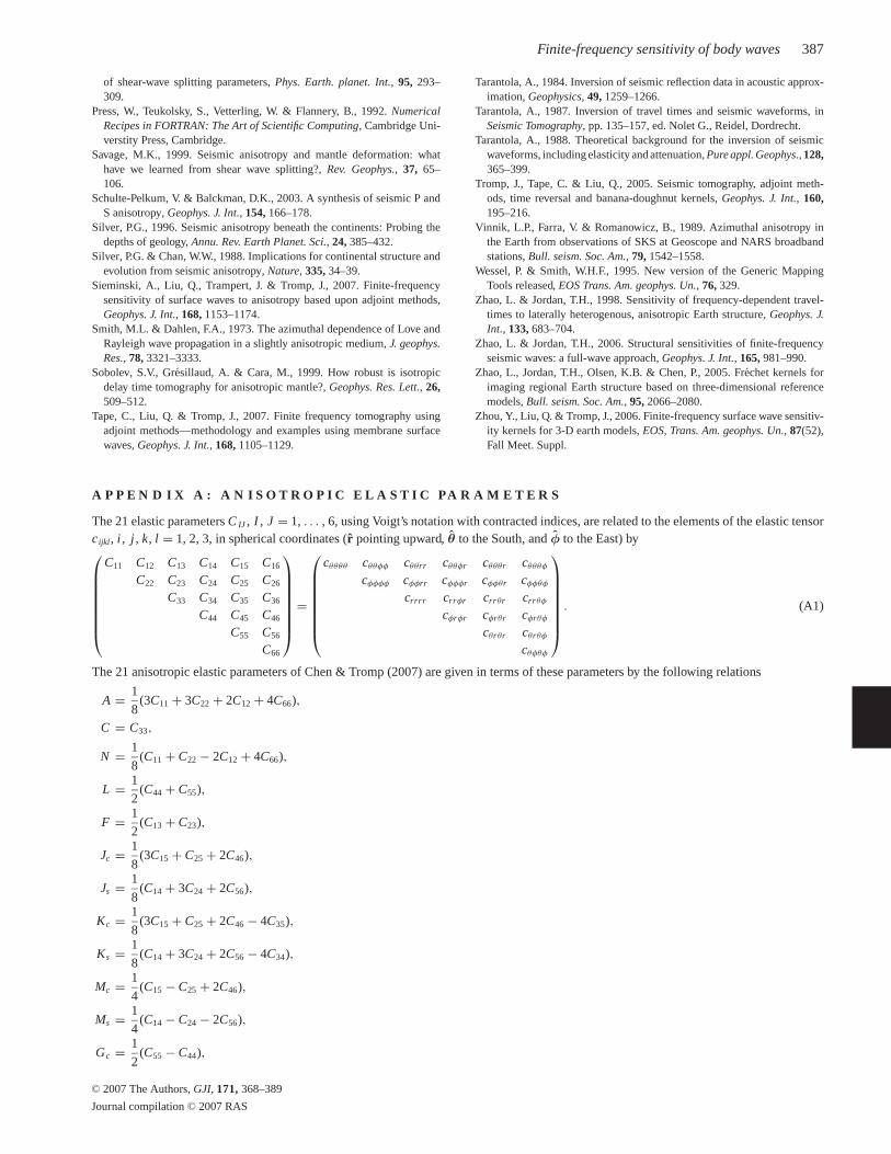
A P P E N D I X A : A N I S O T RO P I C E L A S T I C PA R A M E T E R S
The 21 elastic parameters C IJ , I , J = 1, . . . , 6, using Voigt’s notation with contracted indices, are related to the elements of the elastic tensorcijkl, i , j , k, l = 1, 2, 3, in spherical coordinates (r pointing upward, θ to the South, and φ to the East) by
C11 C12 C13 C14 C15 C16
C22 C23 C24 C25 C26
C33 C34 C35 C36
C44 C45 C46
C55 C56
C66
=
cθθθθ cθθφφ cθθrr cθθφr cθθθr cθθθφ
cφφφφ cφφrr cφφφr cφφθr cφφθφ
crrrr crrφr crrθr crrθφ
cφrφr cφrθr cφrθφ
cθrθr cθrθφ
cθφθφ
. (A1)
The 21 anisotropic elastic parameters of Chen & Tromp (2007) are given in terms of these parameters by the following relations
A = 1
8(3C11 + 3C22 + 2C12 + 4C66),
C = C33,
N = 1
8(C11 + C22 − 2C12 + 4C66),
L = 1
2(C44 + C55),
F = 1
2(C13 + C23),
Jc = 1
8(3C15 + C25 + 2C46),
Js = 1
8(C14 + 3C24 + 2C56),
Kc = 1
8(3C15 + C25 + 2C46 − 4C35),
Ks = 1
8(C14 + 3C24 + 2C56 − 4C34),
Mc = 1
4(C15 − C25 + 2C46),
Ms = 1
4(C14 − C24 − 2C56),
Gc = 1
2(C55 − C44),
C© 2007 The Authors, GJI, 171, 368–389
Journal compilation C© 2007 RAS
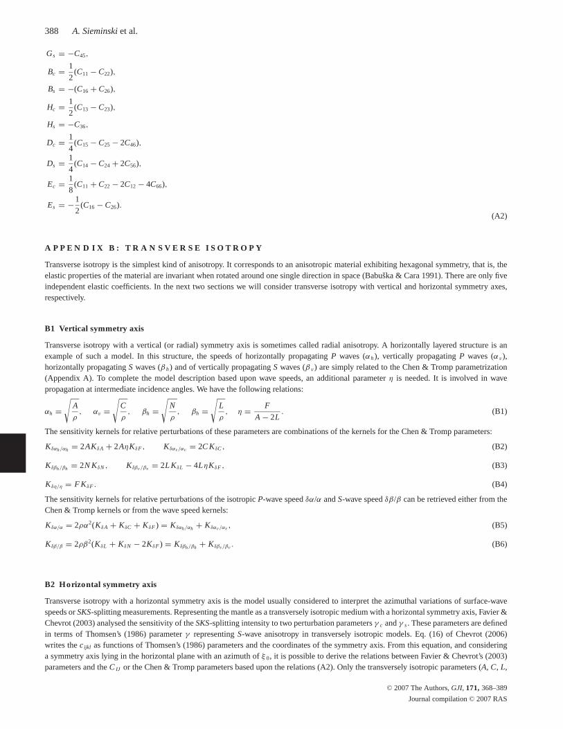
388 A. Sieminski et al.
Gs = −C45,
Bc = 1
2(C11 − C22),
Bs = −(C16 + C26),
Hc = 1
2(C13 − C23),
Hs = −C36,
Dc = 1
4(C15 − C25 − 2C46),
Ds = 1
4(C14 − C24 + 2C56),
Ec = 1
8(C11 + C22 − 2C12 − 4C66),
Es = −1
2(C16 − C26).
(A2)
A P P E N D I X B : T R A N S V E R S E I S O T RO P Y
Transverse isotropy is the simplest kind of anisotropy. It corresponds to an anisotropic material exhibiting hexagonal symmetry, that is, theelastic properties of the material are invariant when rotated around one single direction in space (Babuska & Cara 1991). There are only fiveindependent elastic coefficients. In the next two sections we will consider transverse isotropy with vertical and horizontal symmetry axes,respectively.
B1 Vertical symmetry axis
Transverse isotropy with a vertical (or radial) symmetry axis is sometimes called radial anisotropy. A horizontally layered structure is anexample of such a model. In this structure, the speeds of horizontally propagating P waves (αh), vertically propagating P waves (αv),horizontally propagating S waves (β h) and of vertically propagating S waves (βv) are simply related to the Chen & Tromp parametrization(Appendix A). To complete the model description based upon wave speeds, an additional parameter η is needed. It is involved in wavepropagation at intermediate incidence angles. We have the following relations:
αh =√
A
ρ, αv =
√C
ρ, βh =
√N
ρ, βh =
√L
ρ, η = F
A − 2L. (B1)
The sensitivity kernels for relative perturbations of these parameters are combinations of the kernels for the Chen & Tromp parameters:
Kδαh/αh = 2AKδA + 2AηKδF , Kδαv/αv= 2C KδC , (B2)
Kδβh/βh = 2N KδN , Kδβv/βv= 2L KδL − 4LηKδF , (B3)
Kδη/η = F KδF . (B4)
The sensitivity kernels for relative perturbations of the isotropic P-wave speed δα/α and S-wave speed δβ/β can be retrieved either from theChen & Tromp kernels or from the wave speed kernels:
Kδα/α = 2ρα2(KδA + KδC + KδF ) = Kδαh/αh + Kδαv/αv, (B5)
Kδβ/β = 2ρβ2(KδL + KδN − 2KδF ) = Kδβh/βh + Kδβv/βv. (B6)
B2 Horizontal symmetry axis
Transverse isotropy with a horizontal symmetry axis is the model usually considered to interpret the azimuthal variations of surface-wavespeeds or SKS-splitting measurements. Representing the mantle as a transversely isotropic medium with a horizontal symmetry axis, Favier &Chevrot (2003) analysed the sensitivity of the SKS-splitting intensity to two perturbation parameters γ c and γ s . These parameters are definedin terms of Thomsen’s (1986) parameter γ representing S-wave anisotropy in transversely isotropic models. Eq. (16) of Chevrot (2006)writes the cijkl as functions of Thomsen’s (1986) parameters and the coordinates of the symmetry axis. From this equation, and consideringa symmetry axis lying in the horizontal plane with an azimuth of ξ 0, it is possible to derive the relations between Favier & Chevrot’s (2003)parameters and the C IJ or the Chen & Tromp parameters based upon the relations (A2). Only the transversely isotropic parameters (A, C, L,
C© 2007 The Authors, GJI, 171, 368–389
Journal compilation C© 2007 RAS

Finite-frequency sensitivity of body waves 389
N and F) and the surface-wave parameters (B, H , G and E) are involved in these relations. The body-wave parameters (J , K, M and D) arezero in a transversely isotropic structure with a horizontal symmetry axis. We find that
Gc = −ρβ2γ cos 2ξ0, Gs = ρβ2γ sin 2ξ0, (B7)
where we recognize Favier & Chevrot’s (2003) parameters γ c = γ cos 2ξ 0 and γ s = γ sin 2ξ 0. It is then possible to construct the kernels forFavier & Chevrot’s (2003) parameters from the kernels for the Chen & Tromp parameters:
Kδγc = ρβ2(2KδHc − KδGc ), Kδγs = −ρβ2(2KδHs − KδGs ). (B8)
Our experiments indicate that K δH � 0 for the SKS-splitting intensity. We therefore, may write for this observable
Kδγc � −ρβ2 KδGc , Kδγs � ρβ2 KδGs . (B9)
With these last relations, our results can be readily compared to Favier & Chevrot’s (2003) analysis.
C© 2007 The Authors, GJI, 171, 368–389
Journal compilation C© 2007 RAS