Embed Size (px)
Citation preview
DEPARTMENT OF MANAGEMENT AND ENGINEERING
Finite Element Simulation of Roll Forming
Master Thesis carried out at Solid Mechanics Linköping University
January 2007
Simon Hellborg
LIU-IEI-TEK-A--07/0044--SE
Institute of Technology, Department of Management and Engineering, SE-581 83 Linköping, Sweden

URL för elektronisk version
Titel: Finite Element Simulation of Roll Forming Författare: Simon Hellborg
Sammanfattning A finite element model has been developed to simulate the forming of a channel section profile with the roll forming method. The model has been optimized to experimental results with respect to strains at the edge of the sheet and spring back of the sides of the profile. Finite element models with a coarse mesh have been compared to models with a finer mesh. The models with to fine mesh become instable and a model with a rather coarse mesh was finally chosen. Both the models with shell elements and the models with solid elements have been used in the simulations. The simulations with shell elements gave very good results both for the geometry shape and the strains at the edge of the sheet. The reaction forces at the tools found in the simulations was only half of the reaction forces fond in the experiments. The simulations with the solid element model showed very good results for the reaction forces while the geometry shape of the sheet was really bad. The spring back was much larger in the simulations than in the experiments. The shell element model was chosen because of the excessive spring back with the solid element model. The spring back of the sides of the sheet differs only a few percent between the simulation and the experiment results when using the shell element model. The reaction forces at the tools in the simulation are only half of the reaction forces measured in the experiments but the results from the simulations are linearly proportional to the results in the experiments. The model that finally was chosen describe both the spring back and the strains at the edge of the sheet very well. Like in the experiments there were no signs of wrinkles at the sheet in any of the simulations.
Nyckelord Rullformning, Simulering, Ultrahöghållfast stål, Rollforming, Finite Element Simulation.
Språk Svenska X Engelska Annat (ange nedan)
Rapporttyp Licentiatavhandling X Examensarbete C-uppsats D-uppsats Övrig rapport
ISBN: ISRN: LIU-IEI-TEK-A--07/0044--SE
Serietitel Serienummer/ISSN
Framläggningsdatum 2007-01-12 Publiceringsdatum (elektronisk version)
Avdelning, institution Division, Department Div of Solid Mechanics Dept of Management and Engineering SE-581 83 LINKÖPING

Finite Element Simulation of Roll Forming Author: Simon Hellborg A finite element model has been developed to simulate the forming of a channel section profile with the roll forming method. The model has been optimized to experimental results with respect to strains at the edge of the sheet and spring back of the sides of the profile.
Abstract Roll forming of sheet metal is an important forming process not least in the automotive industry. The increasing use of ultra high strength steel (UHSS) implies an even more extensive use of roll forming since this forming method is suitable in forming UHSS for its ability to obtain small bending radii among other things. Within this study a finite element model has been developed to simulate the forming of a channel section profile with the roll forming method. The model has been optimized to experimental results with respect to strains at the edge of the sheet and spring back of the sides of the profile.
Both models with shell elements and the models with solid elements have been used in the simulations. The simulations with shell elements gave very good results both for the geometry shape and the strains at the edge of the sheet. However the reaction forces at the tools found in the simulations was only half of the reaction forces found in the experiments. The simulations with the solid element model showed very good results for the reaction forces while the geometry shape of the sheet was poor. The spring back was in this case much larger in the simulations than in the experiments. The shell element model was preferred as a reference model and was further analysed because of the excessive spring back with the solid element model. The model that finally was chosen describe both the spring back and the strains at the edge of the sheet very well. Like in the experiments there were no signs of wrinkles at the sheet in any of the simulations.
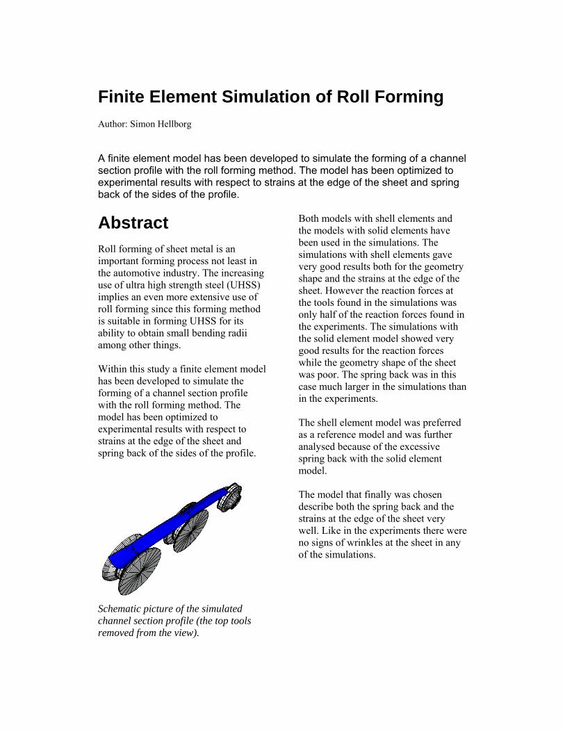
Schematic picture of the simulated channel section profile (the top tools removed from the view).

© Korrosions- och Metallforskningsinstitutet AB (KIMAB)
© Korrosions- och Metallforskningsinstitutet AB (KIMAB)
Table of contents 1. Introduction ................................................................................................................... 1 2. Finite Element Methods ................................................................................................ 4
2.1 Element Definition ................................................................................................ 4 2.2 Comparison of Implicit and Explicit Finite Element Methods ............................. 5
2.2.1 The Explicit Finite Element Method ............................................................. 5 2.2.2 The Implicit Finite Element Method ............................................................. 7 2.2.3 Comparison.................................................................................................... 7
3. Experimental Work ....................................................................................................... 8 3.1 The present roll forming series.............................................................................. 8
4. The Model ................................................................................................................... 10 4.1 Changes in the Model .......................................................................................... 11
4.1.1 Verification of the new tool geometry......................................................... 11 4.2 Description of the model ..................................................................................... 13
4.2.1 The tools ...................................................................................................... 13 4.2.2 The sheet...................................................................................................... 15
4.3 Reference case ..................................................................................................... 16 4.3.1 FEM-method................................................................................................ 16 4.3.2 Element Type............................................................................................... 16 4.3.3 Mesh ............................................................................................................ 18 4.3.4 Mass Scale ................................................................................................... 19 4.3.5 Integration points......................................................................................... 20 4.3.6 Solution time ............................................................................................... 22 4.3.7 Contact Conditions ...................................................................................... 22 4.3.8 Outputs ........................................................................................................ 22 4.3.9 Boundary Conditions................................................................................... 23 4.3.10 Verification of the reference case................................................................ 24
4.4 Materials .............................................................................................................. 25 4.4.1 Materials ...................................................................................................... 25 4.4.2 Spring back .................................................................................................. 26 4.4.3 Reaction forces ............................................................................................ 28 4.4.4 Docol reference material DC01................................................................... 30 4.4.5 HyTens 1200 ............................................................................................... 32 4.4.6 Docol 1200 M.............................................................................................. 34
5. Discussion.................................................................................................................... 36 6. Conclusion................................................................................................................... 37 7. Future work ................................................................................................................. 39 8. Acknowledgements ..................................................................................................... 40 9. Appendix A Tensile test and material data input files to ABAQUS........................... 44 10. Appendix B Results from the simulations............................................................... 54

© Korrosions- och Metallforskningsinstitutet AB (KIMAB)
© Korrosions- och Metallforskningsinstitutet AB (KIMAB)
1
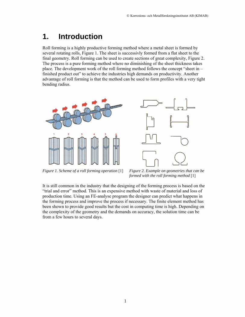
1. Introduction Roll forming is a highly productive forming method where a metal sheet is formed by several rotating rolls, Figure 1. The sheet is successivly formed from a flat sheet to the final geometry. Roll forming can be used to create sections of great complexity, Figure 2. The process is a pure forming method where no diminishing of the sheet thickness takes place. The development work of the roll forming method follows the concept “sheet in – finished product out” to achieve the industries high demands on productivity. Another advantage of roll forming is that the method can be used to form profiles with a very tight bending radius.
Figure 1. Scheme of a roll forming operation [1]
Figure 2. Example on geometries that can be formed with the roll forming method [1]
It is still common in the industry that the designing of the forming process is based on the “trial and error” method. This is an expensive method with waste of material and loss of production time. Using an FE-analyse program the designer can predict what happens in the forming process and improve the process if necessary. The finite element method has been shown to provide good results but the cost in computing time is high. Depending on the complexity of the geometry and the demands on accuracy, the solution time can be from a few hours to several days.
© Korrosions- och Metallforskningsinstitutet AB (KIMAB)
2
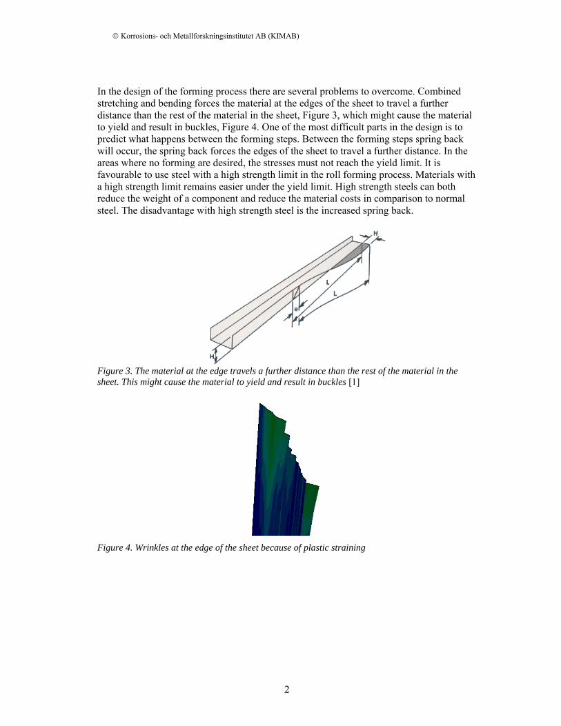
In the design of the forming process there are several problems to overcome. Combined stretching and bending forces the material at the edges of the sheet to travel a further distance than the rest of the material in the sheet, Figure 3, which might cause the material to yield and result in buckles, Figure 4. One of the most difficult parts in the design is to predict what happens between the forming steps. Between the forming steps spring back will occur, the spring back forces the edges of the sheet to travel a further distance. In the areas where no forming are desired, the stresses must not reach the yield limit. It is favourable to use steel with a high strength limit in the roll forming process. Materials with a high strength limit remains easier under the yield limit. High strength steels can both reduce the weight of a component and reduce the material costs in comparison to normal steel. The disadvantage with high strength steel is the increased spring back.
Figure 3. The material at the edge travels a further distance than the rest of the material in the sheet. This might cause the material to yield and result in buckles [1]
Figure 4. Wrinkles at the edge of the sheet because of plastic straining
© Korrosions- och Metallforskningsinstitutet AB (KIMAB)
3
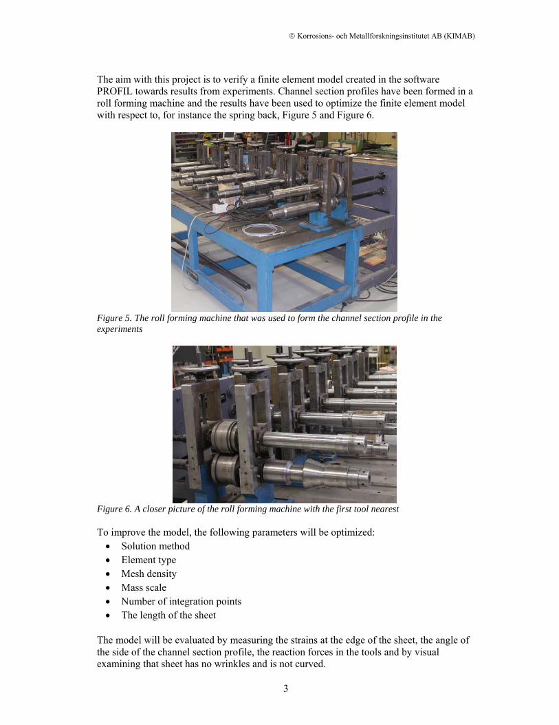
The aim with this project is to verify a finite element model created in the software PROFIL towards results from experiments. Channel section profiles have been formed in a roll forming machine and the results have been used to optimize the finite element model with respect to, for instance the spring back, Figure 5 and Figure 6.
Figure 5. The roll forming machine that was used to form the channel section profile in the experiments
Figure 6. A closer picture of the roll forming machine with the first tool nearest To improve the model, the following parameters will be optimized: • Solution method • Element type • Mesh density • Mass scale • Number of integration points • The length of the sheet
The model will be evaluated by measuring the strains at the edge of the sheet, the angle of the side of the channel section profile, the reaction forces in the tools and by visual examining that sheet has no wrinkles and is not curved.

© Korrosions- och Metallforskningsinstitutet AB (KIMAB)
4
2. Finite Element Methods
2.1 Element definition For a sheet, where the thickness is significantly smaller than the other sides, the stress in the thickness direction can be neglected. When the thickness is small and the stress in the thickness direction is negligible, shell and membrane elements can be used for modelling the sheet. The finite element program ABAQUS uses a surface to describe the contact and the interactions between the tools and the sheet in the model [2]. The surface in a shell element model can be defined in three different ways, by a node-based surface, element-based surface or an analytic curve. The element-based surface is continuous and therefore it contains more intrinsic information than a discontinuous nodal-based surface. The element-based surface gives in comparison to a nodal-based surface a more accurate contact calculation. The roll forming software PROFIL generates the sheet with a node-based surface as default. When a surface is defined based on the nodes, it will by default be placed in the centre plan. An element-based surface was placed at the actual surface of the sheet. The user of the FE-program must be aware of the surface definition when defining the contact conditions. ABAQUS uses the overclosure between the tools and the surface to calculate the contact pressure between the tools to the sheet surface. To verify the contact pressure the user must know the distance between the defined surface and the actual surface of the sheet.
© Korrosions- och Metallforskningsinstitutet AB (KIMAB)
5
2.2 Comparison of Implicit and Explicit Finite Element Methods
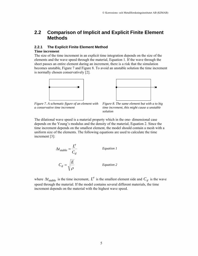
2.2.1 The Explicit Finite Element Method Time increment The size of the time increment in an explicit time integration depends on the size of the elements and the wave speed through the material, Equation 1. If the wave through the sheet passes an entire element during an increment, there is a risk that the simulation becomes unstable, Figure 7 and Figure 8. To avoid an unstable solution the time increment is normally chosen conservatively [2].
Figure 7. A schematic figure of an element with a conservative time increment
Figure 8. The same element but with a to big time increment, this might cause a unstable solution
The dilational wave speed is a material property which in the one- dimensional case depends on the Young’s modulus and the density of the material, Equation 2. Since the time increment depends on the smallest element, the model should contain a mesh with a uniform size of the elements. The following equations are used to calculate the time increment [3]:
d
e
stable CLt =Δ
Equation 1
ρECd =
Equation 2
where stabletΔ is the time increment, eL is the smallest element side and dC is the wave speed through the material. If the model contains several different materials, the time increment depends on the material with the highest wave speed.
© Korrosions- och Metallforskningsinstitutet AB (KIMAB)
6
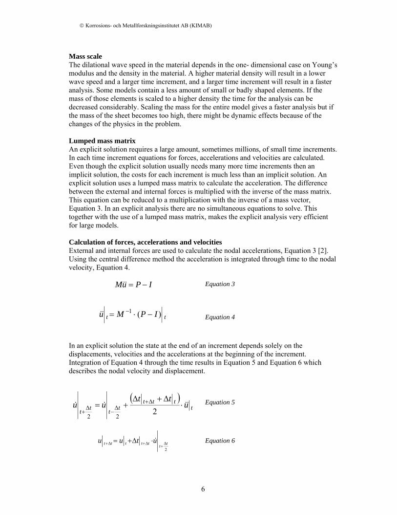
Mass scale The dilational wave speed in the material depends in the one- dimensional case on Young’s modulus and the density in the material. A higher material density will result in a lower wave speed and a larger time increment, and a larger time increment will result in a faster analysis. Some models contain a less amount of small or badly shaped elements. If the mass of those elements is scaled to a higher density the time for the analysis can be decreased considerably. Scaling the mass for the entire model gives a faster analysis but if the mass of the sheet becomes too high, there might be dynamic effects because of the changes of the physics in the problem. Lumped mass matrix An explicit solution requires a large amount, sometimes millions, of small time increments. In each time increment equations for forces, accelerations and velocities are calculated. Even though the explicit solution usually needs many more time increments then an implicit solution, the costs for each increment is much less than an implicit solution. An explicit solution uses a lumped mass matrix to calculate the acceleration. The difference between the external and internal forces is multiplied with the inverse of the mass matrix. This equation can be reduced to a multiplication with the inverse of a mass vector, Equation 3. In an explicit analysis there are no simultaneous equations to solve. This together with the use of a lumped mass matrix, makes the explicit analysis very efficient for large models. Calculation of forces, accelerations and velocities External and internal forces are used to calculate the nodal accelerations, Equation 3 [2]. Using the central difference method the acceleration is integrated through time to the nodal velocity, Equation 4.
IPuM −=&& Equation 3
tt IPMu )(1 −⋅= −&& Equation 4
In an explicit solution the state at the end of an increment depends solely on the displacements, velocities and the accelerations at the beginning of the increment. Integration of Equation 4 through the time results in Equation 5 and Equation 6 which describes the nodal velocity and displacement.
( )t
ttttttt
utt
uu &&&& ⋅Δ+Δ
+= Δ+Δ
−Δ
+ 222
Equation 5
2ttttttt utuu Δ
+Δ+Δ+ ⋅Δ+= &
Equation 6
© Korrosions- och Metallforskningsinstitutet AB (KIMAB)
7
2.2.2 The Implicit Finite Element Method Time step Implicit solutions, like the explicit solutions, use the equilibrium between external and internal forces to calculate the nodal accelerations. The distinction between the methods is in the way that the nodal accelerations are solved. The implicit solution determines the nodal acceleration by solving a nonlinear equation system in each time increment. Solving those equations has a relative high computational cost for large models relative the explicit way to solve the nodal acceleration. On the other hand, since the implicit method usually is unconditionally stable, it can use larger time increments. The size of a time increment for an implicit solution depends on the desired accuracy of the solution. ABAQUS/standard uses the full Newton iterative solution method, which means that it tries to find a dynamic equilibrium at the end of the increment at the same time as it computes the nodal displacements. Convergence of tolerance In an implicit solution, the relative error has a quadratic convergence for a linear problem, but a nonlinear problem needs several more iterations to converge to the user predetermined tolerance. A highly discontinuous problem might need shorter time increments for the solution to converge, this will result in a very high computational cost. 2.2.3 Comparison Contact conditions Complex contact conditions including interactions between several bodies give a highly discontinuous model that is more suitable for explicit analysis then for an implicit analysis. The short time increments in the explicit solution make the explicit solution well suited for rapidly changes of the contact conditions while an implicit solution might fail to converge. Accuracy and calculation time For highly nonlinear problems the implicit solution might not converge. In a problem with a lot of contacts the solution will probably not converge with the implicit solution method. The solution time for the implicit solution method increases with the square of the wave front times the number of degrees of freedom while the solution time for the explicit solver increases linearly with a factor eight for a 2-dimensional analysis [3].
© Korrosions- och Metallforskningsinstitutet AB (KIMAB)
8
3. Experimental work
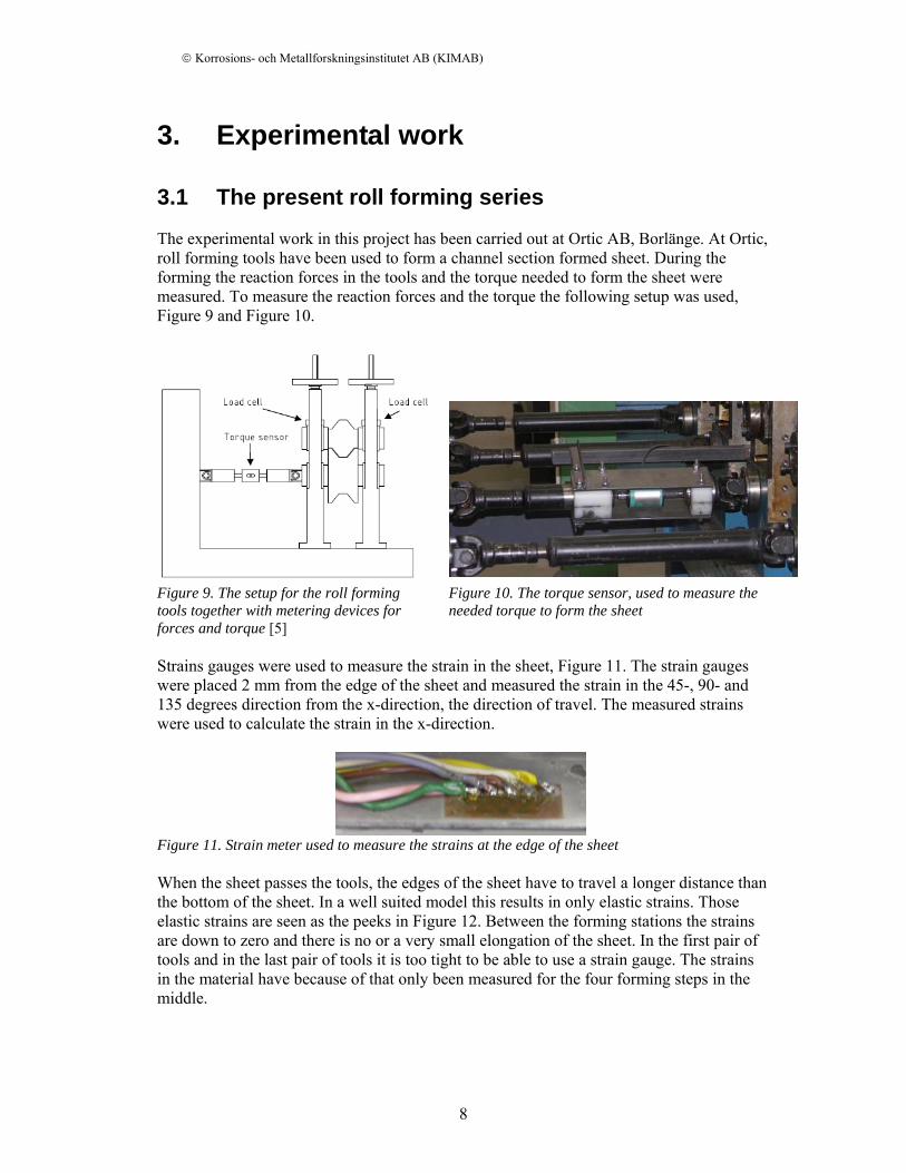
3.1 The present roll forming series The experimental work in this project has been carried out at Ortic AB, Borlänge. At Ortic, roll forming tools have been used to form a channel section formed sheet. During the forming the reaction forces in the tools and the torque needed to form the sheet were measured. To measure the reaction forces and the torque the following setup was used, Figure 9 and Figure 10.
Figure 9. The setup for the roll forming tools together with metering devices for forces and torque [5]
Figure 10. The torque sensor, used to measure the needed torque to form the sheet
Strains gauges were used to measure the strain in the sheet, Figure 11. The strain gauges were placed 2 mm from the edge of the sheet and measured the strain in the 45-, 90- and 135 degrees direction from the x-direction, the direction of travel. The measured strains were used to calculate the strain in the x-direction.
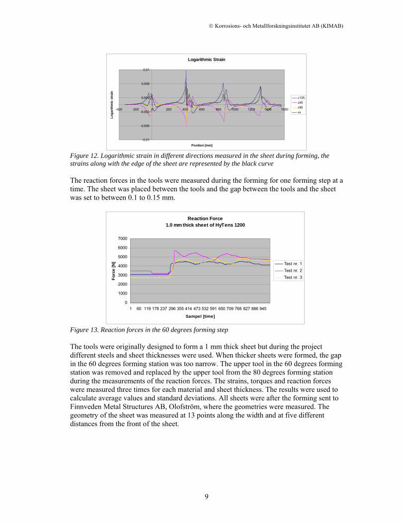
Figure 11. Strain meter used to measure the strains at the edge of the sheet When the sheet passes the tools, the edges of the sheet have to travel a longer distance than the bottom of the sheet. In a well suited model this results in only elastic strains. Those elastic strains are seen as the peeks in Figure 12. Between the forming stations the strains are down to zero and there is no or a very small elongation of the sheet. In the first pair of tools and in the last pair of tools it is too tight to be able to use a strain gauge. The strains in the material have because of that only been measured for the four forming steps in the middle.
© Korrosions- och Metallforskningsinstitutet AB (KIMAB)
9
Logarithmic Strain
-0,01
-0,006
-0,002
0,002
0,006
0,01
-400 -200 0 200 400 600 800 1000 1200 1400 1600
Position [mm]
Loga
rithm
ic s
train
ε135ε45ε90εx
Figure 12. Logarithmic strain in different directions measured in the sheet during forming, the strains along with the edge of the sheet are represented by the black curve The reaction forces in the tools were measured during the forming for one forming step at a time. The sheet was placed between the tools and the gap between the tools and the sheet was set to between 0.1 to 0.15 mm.
Reaction Force1.0 mm thick sheet of HyTens 1200
0
1000
2000
3000
4000
5000
6000
7000
1 60 119 178 237 296 355 414 473 532 591 650 709 768 827 886 945
Sampel [time]
Forc
e [N
] Test nr. 1Test nr. 2Test nr. 3
Figure 13. Reaction forces in the 60 degrees forming step The tools were originally designed to form a 1 mm thick sheet but during the project different steels and sheet thicknesses were used. When thicker sheets were formed, the gap in the 60 degrees forming station was too narrow. The upper tool in the 60 degrees forming station was removed and replaced by the upper tool from the 80 degrees forming station during the measurements of the reaction forces. The strains, torques and reaction forces were measured three times for each material and sheet thickness. The results were used to calculate average values and standard deviations. All sheets were after the forming sent to Finnveden Metal Structures AB, Olofström, where the geometries were measured. The geometry of the sheet was measured at 13 points along the width and at five different distances from the front of the sheet.
© Korrosions- och Metallforskningsinstitutet AB (KIMAB)
10
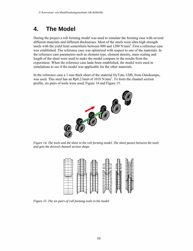
4. The Model During the project a roll forming model was used to simulate the forming case with several different materials and different thicknesses. Most of the steels were ultra high strength steels with the yield limit somewhere between 800 and 1200 N/mm2. First a reference case was established. The reference case was optimized with respect to one of the materials. In the reference case parameters such as element type, element density, mass scaling and length of the sheet were used to make the model compare to the results from the experiment. When the reference case hade been established, the model were used in simulations to see if the model was applicable for the other materials. In the reference case a 1 mm thick sheet of the material HyTens 1200, from Outokumpu, was used. This steel has an Rp0.2 limit of 1018 N/mm2. To form the channel section profile, six pairs of tools were used, Figure 14 and Figure 15.
Figure 14. The tools and the sheet in the roll forming model. The sheet passes between the tools and gets the desired channel section shape
Figure 15. The six pairs of roll forming tools in the model
© Korrosions- och Metallforskningsinstitutet AB (KIMAB)
11
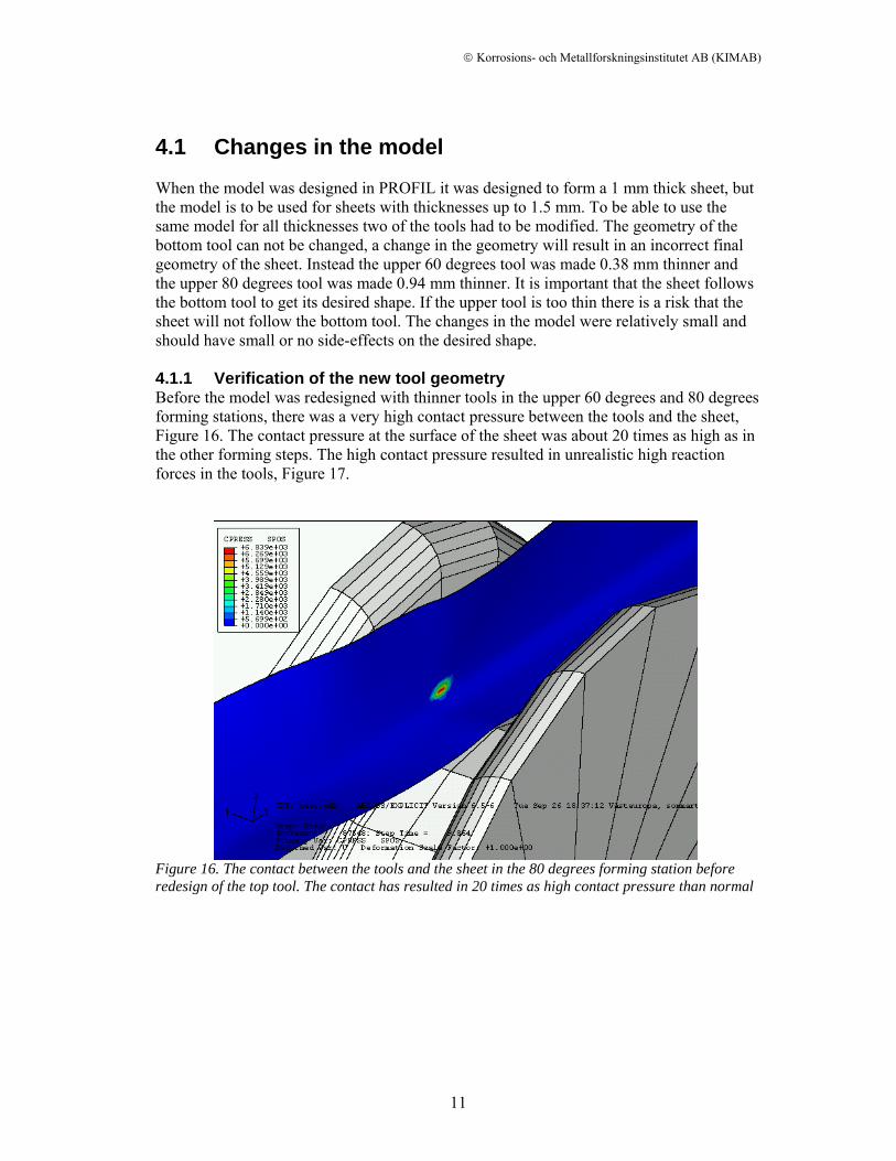
4.1 Changes in the model When the model was designed in PROFIL it was designed to form a 1 mm thick sheet, but the model is to be used for sheets with thicknesses up to 1.5 mm. To be able to use the same model for all thicknesses two of the tools had to be modified. The geometry of the bottom tool can not be changed, a change in the geometry will result in an incorrect final geometry of the sheet. Instead the upper 60 degrees tool was made 0.38 mm thinner and the upper 80 degrees tool was made 0.94 mm thinner. It is important that the sheet follows the bottom tool to get its desired shape. If the upper tool is too thin there is a risk that the sheet will not follow the bottom tool. The changes in the model were relatively small and should have small or no side-effects on the desired shape. 4.1.1 Verification of the new tool geometry Before the model was redesigned with thinner tools in the upper 60 degrees and 80 degrees forming stations, there was a very high contact pressure between the tools and the sheet, Figure 16. The contact pressure at the surface of the sheet was about 20 times as high as in the other forming steps. The high contact pressure resulted in unrealistic high reaction forces in the tools, Figure 17.
Figure 16. The contact between the tools and the sheet in the 80 degrees forming station before redesign of the top tool. The contact has resulted in 20 times as high contact pressure than normal
© Korrosions- och Metallforskningsinstitutet AB (KIMAB)
12
Reaction Forces
-20000
0
20000
40000
60000
80000
100000
1 3 5 7 9 11 13
Time (s)
Reac
tion
forc
es (N
)
20 degree40 degree60 degree80 degree
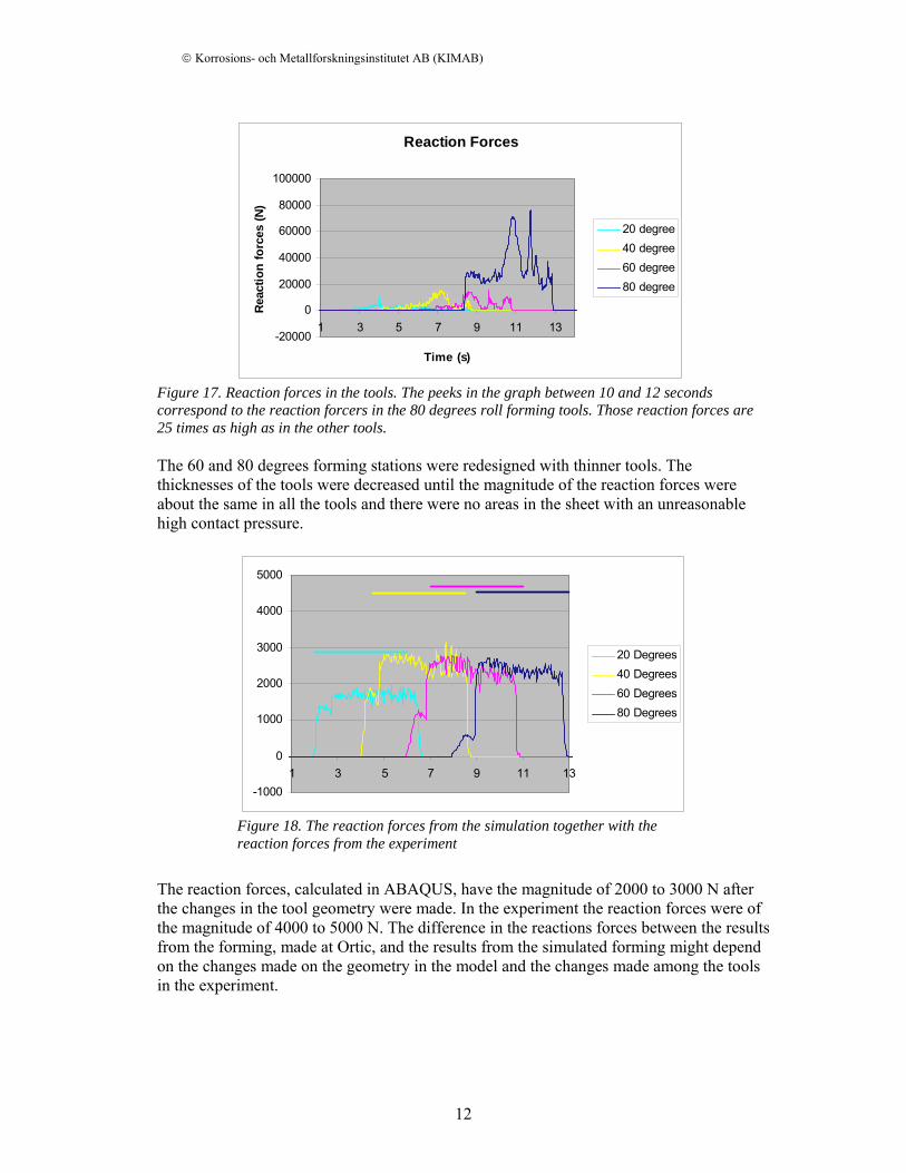
Figure 17. Reaction forces in the tools. The peeks in the graph between 10 and 12 seconds correspond to the reaction forcers in the 80 degrees roll forming tools. Those reaction forces are 25 times as high as in the other tools. The 60 and 80 degrees forming stations were redesigned with thinner tools. The thicknesses of the tools were decreased until the magnitude of the reaction forces were about the same in all the tools and there were no areas in the sheet with an unreasonable high contact pressure.
-1000
0
1000
2000
3000
4000
5000
1 3 5 7 9 11 13
20 Degrees40 Degrees60 Degrees80 Degrees
Figure 18. The reaction forces from the simulation together with the reaction forces from the experiment
The reaction forces, calculated in ABAQUS, have the magnitude of 2000 to 3000 N after the changes in the tool geometry were made. In the experiment the reaction forces were of the magnitude of 4000 to 5000 N. The difference in the reactions forces between the results from the forming, made at Ortic, and the results from the simulated forming might depend on the changes made on the geometry in the model and the changes made among the tools in the experiment.
© Korrosions- och Metallforskningsinstitutet AB (KIMAB)
13
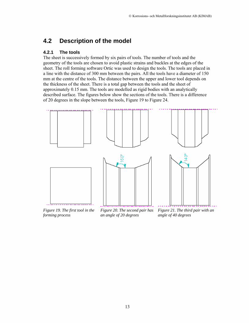
4.2 Description of the model 4.2.1 The tools The sheet is successively formed by six pairs of tools. The number of tools and the geometry of the tools are chosen to avoid plastic strains and buckles at the edges of the sheet. The roll forming software Ortic was used to design the tools. The tools are placed in a line with the distance of 300 mm between the pairs. All the tools have a diameter of 150 mm at the centre of the tools. The distance between the upper and lower tool depends on the thickness of the sheet. There is a total gap between the tools and the sheet of approximately 0.15 mm. The tools are modelled as rigid bodies with an analytically described surface. The figures below show the sections of the tools. There is a difference of 20 degrees in the slope between the tools, Figure 19 to Figure 24.
Figure 19. The first tool in the forming process
Figure 20. The second pair has an angle of 20 degrees
Figure 21. The third pair with an angle of 40 degrees
© Korrosions- och Metallforskningsinstitutet AB (KIMAB)
14
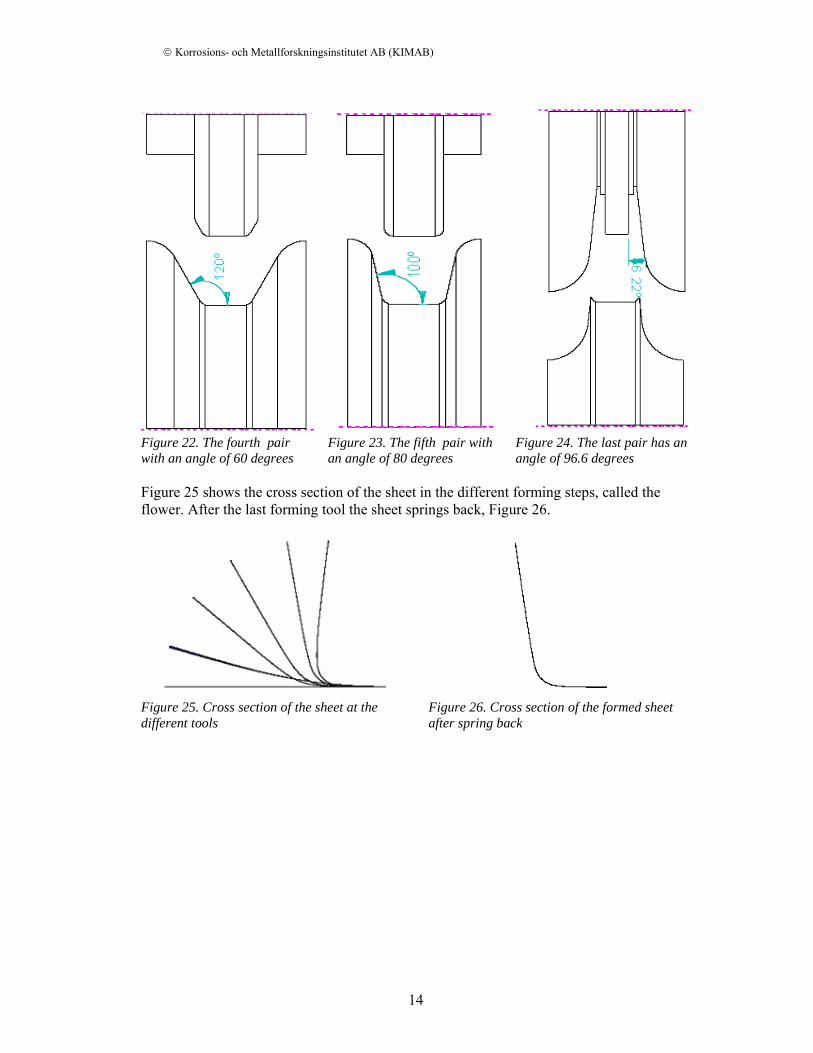
Figure 22. The fourth pair with an angle of 60 degrees
Figure 23. The fifth pair with an angle of 80 degrees
Figure 24. The last pair has an angle of 96.6 degrees
Figure 25 shows the cross section of the sheet in the different forming steps, called the flower. After the last forming tool the sheet springs back, Figure 26.
Figure 25. Cross section of the sheet at the different tools
Figure 26. Cross section of the formed sheet after spring back
© Korrosions- och Metallforskningsinstitutet AB (KIMAB)
15
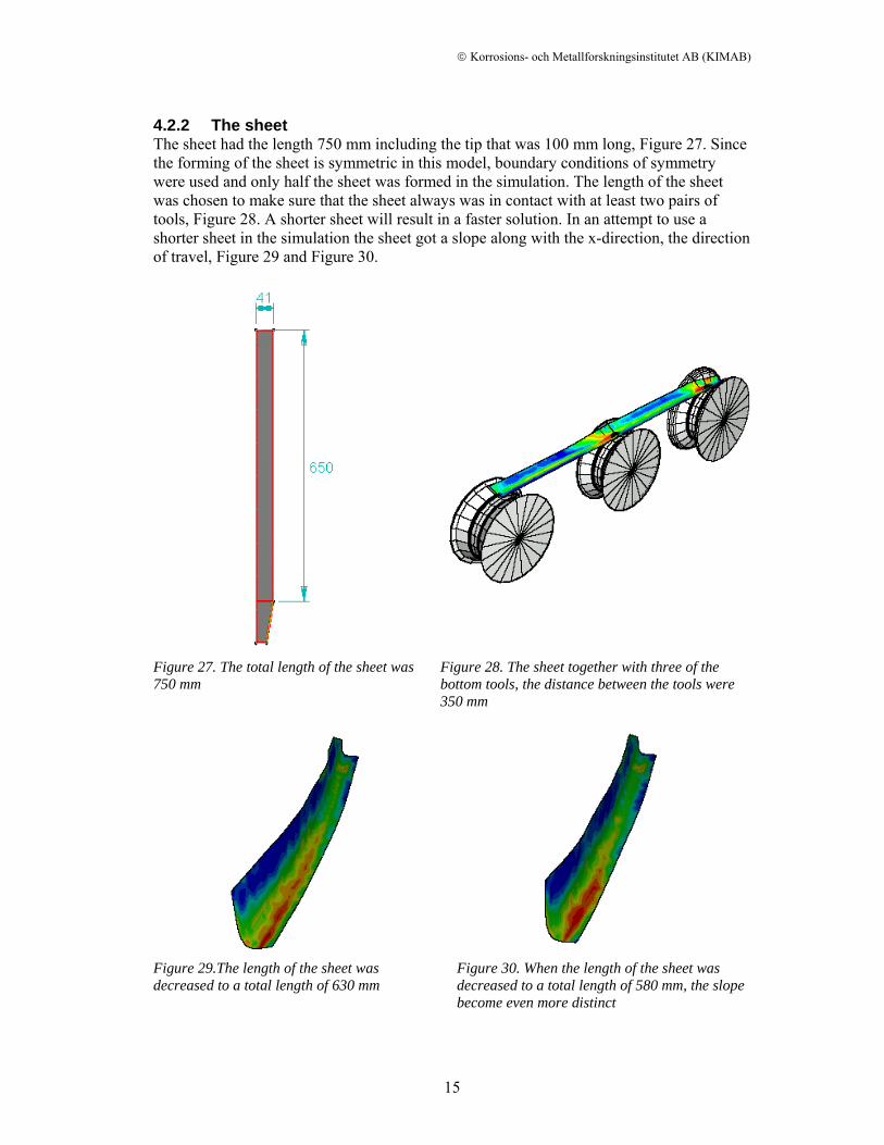
4.2.2 The sheet The sheet had the length 750 mm including the tip that was 100 mm long, Figure 27. Since the forming of the sheet is symmetric in this model, boundary conditions of symmetry were used and only half the sheet was formed in the simulation. The length of the sheet was chosen to make sure that the sheet always was in contact with at least two pairs of tools, Figure 28. A shorter sheet will result in a faster solution. In an attempt to use a shorter sheet in the simulation the sheet got a slope along with the x-direction, the direction of travel, Figure 29 and Figure 30.
Figure 27. The total length of the sheet was 750 mm
Figure 28. The sheet together with three of the bottom tools, the distance between the tools were 350 mm
Figure 29.The length of the sheet was decreased to a total length of 630 mm
Figure 30. When the length of the sheet was decreased to a total length of 580 mm, the slope become even more distinct
© Korrosions- och Metallforskningsinstitutet AB (KIMAB)
16
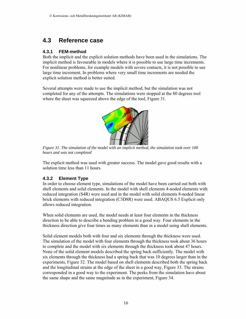
4.3 Reference case 4.3.1 FEM-method Both the implicit and the explicit solution methods have been used in the simulations. The implicit method is favourable in models where it is possible to use large time increments. For nonlinear problems, for example models with severe contacts, it is not possible to use large time increment. In problems where very small time increments are needed the explicit solution method is better suited. Several attempts were made to use the implicit method, but the simulation was not completed for any of the attempts. The simulations were stopped at the 80 degrees tool where the sheet was squeezed above the edge of the tool, Figure 31.
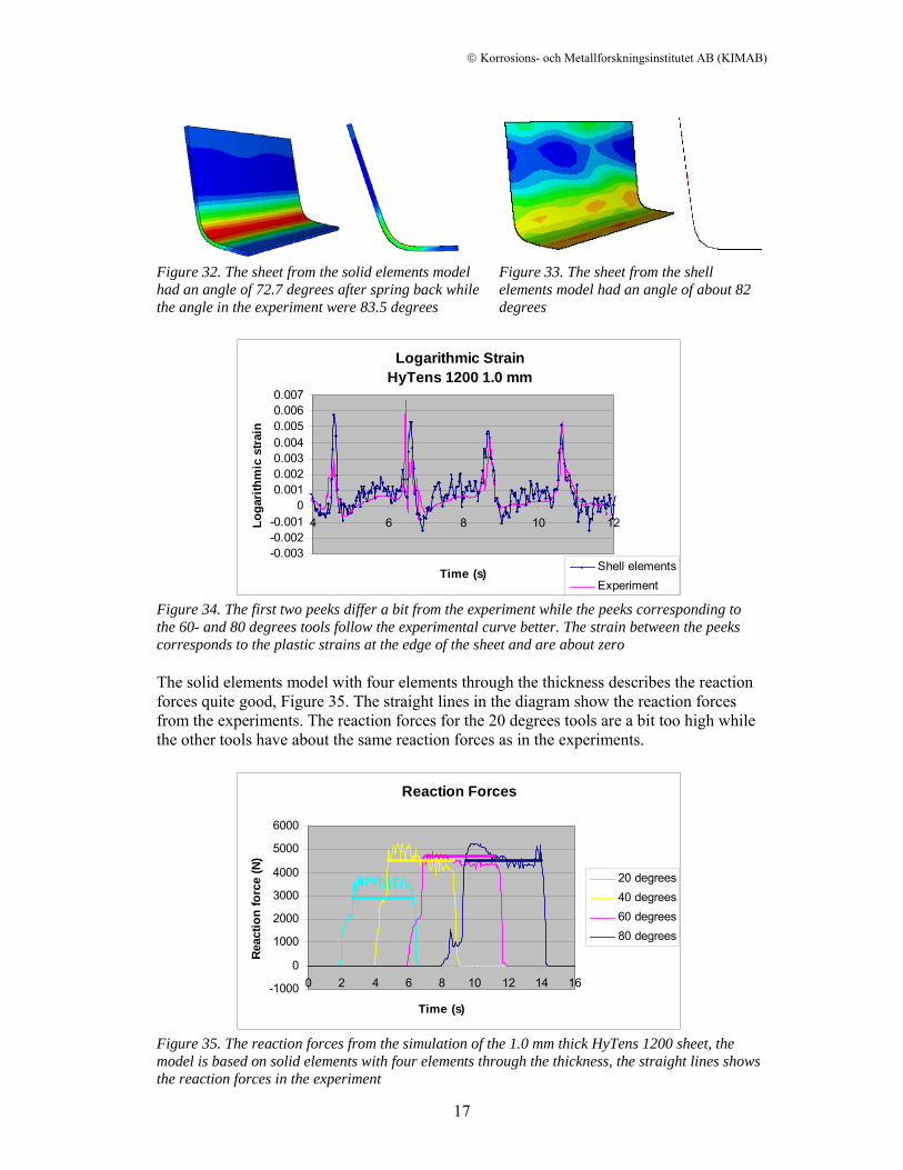
Figure 31. The simulation of the model with an implicit method, the simulation took over 100 hours and was not completed The explicit method was used with greater success. The model gave good results with a solution time less than 11 hours. 4.3.2 Element Type In order to choose element type, simulations of the model have been carried out both with shell elements and solid elements. In the model with shell elements 4-noded elements with reduced integration (S4R) were used and in the model with solid elements 8-noded linear brick elements with reduced integration (C3D8R) were used. ABAQUS 6.5 Explicit only allows reduced integration. When solid elements are used, the model needs at least four elements in the thickness direction to be able to describe a bending problem in a good way. Four elements in the thickness direction give four times as many elements than in a model using shell elements. Solid element models both with four and six elements through the thickness were used. The simulation of the model with four elements through the thickness took about 36 hours to complete and the model with six elements through the thickness took about 47 hours. None of the solid element models described the spring back sufficiently. The model with six elements through the thickness had a spring back that was 10 degrees larger than in the experiments, Figure 32. The model based on shell elements described both the spring back and the longitudinal strains at the edge of the sheet in a good way, Figure 33. The strains corresponded in a good way to the experiment. The peeks from the simulation have about the same shape and the same magnitude as in the experiment, Figure 34.
© Korrosions- och Metallforskningsinstitutet AB (KIMAB)
17
Figure 32. The sheet from the solid elements model had an angle of 72.7 degrees after spring back while the angle in the experiment were 83.5 degrees
Figure 33. The sheet from the shell elements model had an angle of about 82 degrees
Logarithmic StrainHyTens 1200 1.0 mm
-0.003-0.002-0.001
00.0010.0020.0030.0040.0050.0060.007
4 6 8 10 12
Time (s)
Loga
rith
mic
stra
in
Shell elementsExperiment
Figure 34. The first two peeks differ a bit from the experiment while the peeks corresponding to the 60- and 80 degrees tools follow the experimental curve better. The strain between the peeks corresponds to the plastic strains at the edge of the sheet and are about zero The solid elements model with four elements through the thickness describes the reaction forces quite good, Figure 35. The straight lines in the diagram show the reaction forces from the experiments. The reaction forces for the 20 degrees tools are a bit too high while the other tools have about the same reaction forces as in the experiments.
Reaction Forces
-1000
0
1000
2000
3000
4000
5000
6000
0 2 4 6 8 10 12 14 16
Time (s)
Reac
tion
forc
e (N
)
20 degrees40 degrees60 degrees80 degrees
Figure 35. The reaction forces from the simulation of the 1.0 mm thick HyTens 1200 sheet, the model is based on solid elements with four elements through the thickness, the straight lines shows the reaction forces in the experiment
© Korrosions- och Metallforskningsinstitutet AB (KIMAB)
18
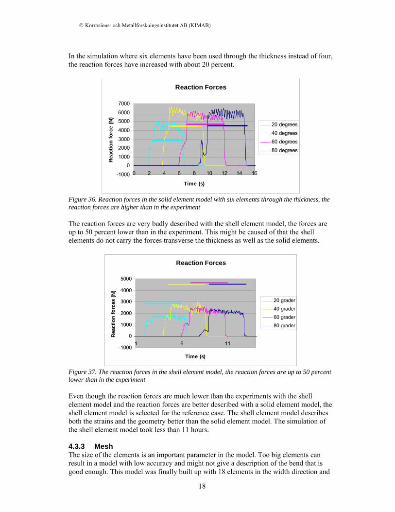
In the simulation where six elements have been used through the thickness instead of four, the reaction forces have increased with about 20 percent.
Reaction Forces
-1000
01000
20003000
4000
50006000
7000
0 2 4 6 8 10 12 14 16
Time (s)
Reac
tion
forc
e (N
)
20 degrees40 degrees60 degrees80 degrees
Figure 36. Reaction forces in the solid element model with six elements through the thickness, the reaction forces are higher than in the experiment The reaction forces are very badly described with the shell element model, the forces are up to 50 percent lower than in the experiment. This might be caused of that the shell elements do not carry the forces transverse the thickness as well as the solid elements.
Reaction Forces
-1000
0
1000
2000
3000
4000
5000
1 6 11
Time (s)
Rea
ctio
n fo
rces
(N)
20 grader40 grader60 grader80 grader
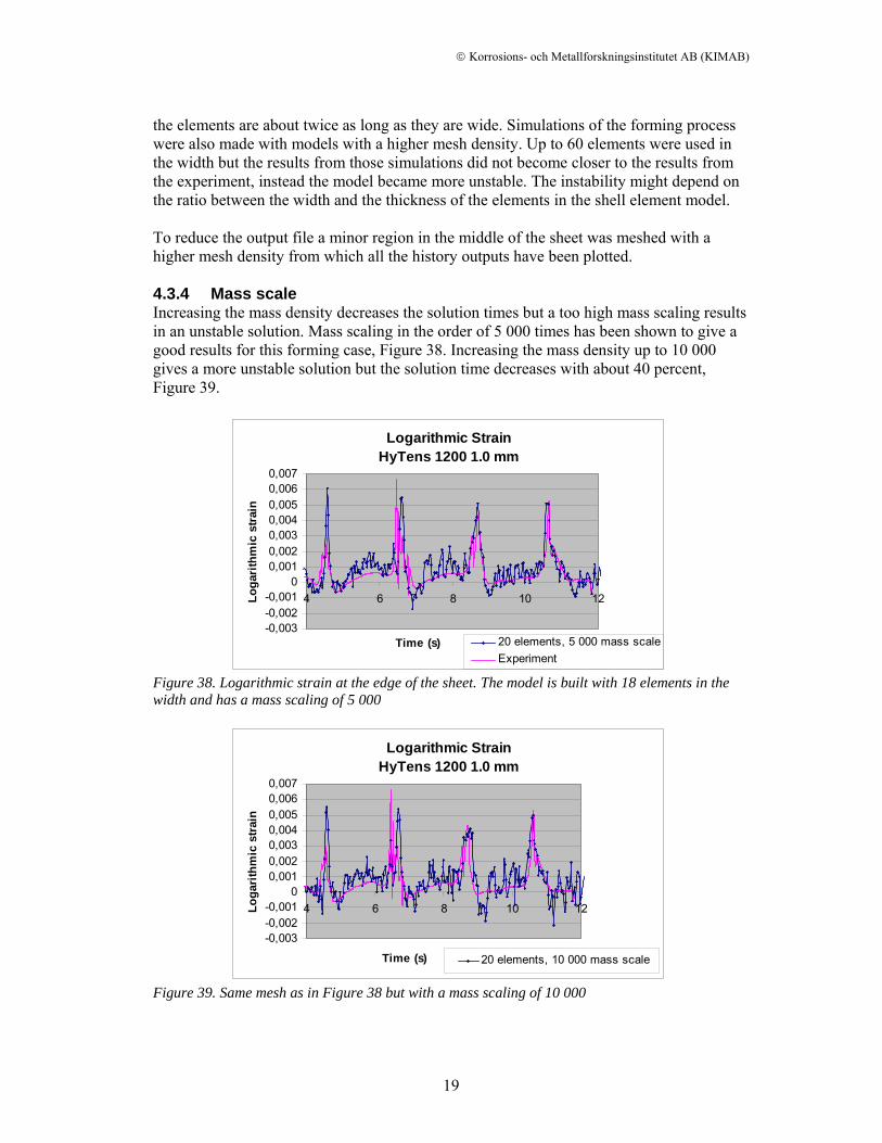
Figure 37. The reaction forces in the shell element model, the reaction forces are up to 50 percent lower than in the experiment Even though the reaction forces are much lower than the experiments with the shell element model and the reaction forces are better described with a solid element model, the shell element model is selected for the reference case. The shell element model describes both the strains and the geometry better than the solid element model. The simulation of the shell element model took less than 11 hours. 4.3.3 Mesh The size of the elements is an important parameter in the model. Too big elements can result in a model with low accuracy and might not give a description of the bend that is good enough. This model was finally built up with 18 elements in the width direction and
© Korrosions- och Metallforskningsinstitutet AB (KIMAB)
19
the elements are about twice as long as they are wide. Simulations of the forming process were also made with models with a higher mesh density. Up to 60 elements were used in the width but the results from those simulations did not become closer to the results from the experiment, instead the model became more unstable. The instability might depend on the ratio between the width and the thickness of the elements in the shell element model. To reduce the output file a minor region in the middle of the sheet was meshed with a higher mesh density from which all the history outputs have been plotted. 4.3.4 Mass scale Increasing the mass density decreases the solution times but a too high mass scaling results in an unstable solution. Mass scaling in the order of 5 000 times has been shown to give a good results for this forming case, Figure 38. Increasing the mass density up to 10 000 gives a more unstable solution but the solution time decreases with about 40 percent, Figure 39.
Logarithmic StrainHyTens 1200 1.0 mm
-0,003-0,002-0,001
00,0010,0020,0030,0040,0050,0060,007
4 6 8 10 12
Time (s)
Loga
rith
mic
stra
in
20 elements, 5 000 mass scaleExperiment
Figure 38. Logarithmic strain at the edge of the sheet. The model is built with 18 elements in the width and has a mass scaling of 5 000
Logarithmic StrainHyTens 1200 1.0 mm
-0,003-0,002-0,001
00,0010,0020,0030,0040,0050,0060,007
4 6 8 10 12
Time (s)
Loga
rithm
ic s
trai
n
20 elements, 10 000 mass scale
Figure 39. Same mesh as in Figure 38 but with a mass scaling of 10 000
© Korrosions- och Metallforskningsinstitutet AB (KIMAB)
20
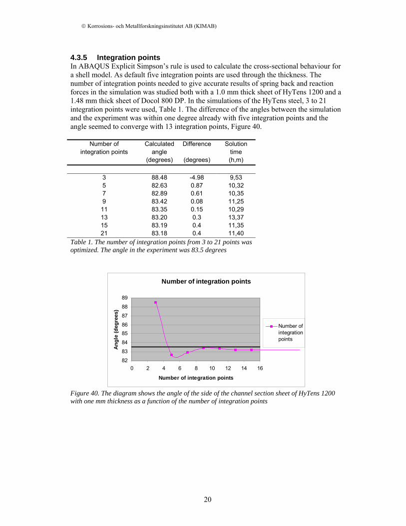
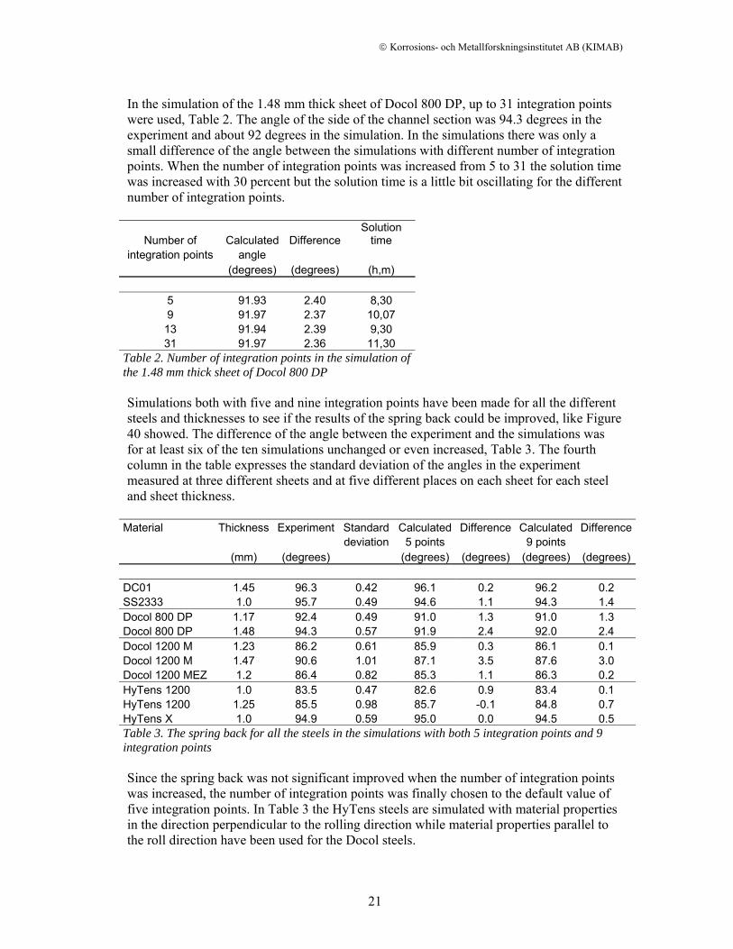
4.3.5 Integration points In ABAQUS Explicit Simpson’s rule is used to calculate the cross-sectional behaviour for a shell model. As default five integration points are used through the thickness. The number of integration points needed to give accurate results of spring back and reaction forces in the simulation was studied both with a 1.0 mm thick sheet of HyTens 1200 and a 1.48 mm thick sheet of Docol 800 DP. In the simulations of the HyTens steel, 3 to 21 integration points were used, Table 1. The difference of the angles between the simulation and the experiment was within one degree already with five integration points and the angle seemed to converge with 13 integration points, Figure 40.
Number of Calculated Difference Solution integration points angle time
(degrees) (degrees) (h,m)
3 88.48 -4.98 9,53 5 82.63 0.87 10,32 7 82.89 0.61 10,35 9 83.42 0.08 11,25
11 83.35 0.15 10,29 13 83.20 0.3 13,37 15 83.19 0.4 11,35 21 83.18 0.4 11,40
Table 1. The number of integration points from 3 to 21 points was optimized. The angle in the experiment was 83.5 degrees
Number of integration points
82
83
84
8586
87
88
89
0 2 4 6 8 10 12 14 16
Number of integration points
Ang
le (d
egre
es)
Number ofintegrationpoints
Figure 40. The diagram shows the angle of the side of the channel section sheet of HyTens 1200 with one mm thickness as a function of the number of integration points
© Korrosions- och Metallforskningsinstitutet AB (KIMAB)
21
In the simulation of the 1.48 mm thick sheet of Docol 800 DP, up to 31 integration points were used, Table 2. The angle of the side of the channel section was 94.3 degrees in the experiment and about 92 degrees in the simulation. In the simulations there was only a small difference of the angle between the simulations with different number of integration points. When the number of integration points was increased from 5 to 31 the solution time was increased with 30 percent but the solution time is a little bit oscillating for the different number of integration points.
Number of Calculated Difference Solution
time integration points angle
(degrees) (degrees) (h,m)
5 91.93 2.40 8,30 9 91.97 2.37 10,07 13 91.94 2.39 9,30 31 91.97 2.36 11,30
Table 2. Number of integration points in the simulation of the 1.48 mm thick sheet of Docol 800 DP Simulations both with five and nine integration points have been made for all the different steels and thicknesses to see if the results of the spring back could be improved, like Figure 40 showed. The difference of the angle between the experiment and the simulations was for at least six of the ten simulations unchanged or even increased, Table 3. The fourth column in the table expresses the standard deviation of the angles in the experiment measured at three different sheets and at five different places on each sheet for each steel and sheet thickness.
Material Thickness Experiment Standard Calculated Difference Calculated Difference deviation 5 points 9 points (mm) (degrees) (degrees) (degrees) (degrees) (degrees)
DC01 1.45 96.3 0.42 96.1 0.2 96.2 0.2 SS2333 1.0 95.7 0.49 94.6 1.1 94.3 1.4 Docol 800 DP 1.17 92.4 0.49 91.0 1.3 91.0 1.3 Docol 800 DP 1.48 94.3 0.57 91.9 2.4 92.0 2.4 Docol 1200 M 1.23 86.2 0.61 85.9 0.3 86.1 0.1 Docol 1200 M 1.47 90.6 1.01 87.1 3.5 87.6 3.0 Docol 1200 MEZ 1.2 86.4 0.82 85.3 1.1 86.3 0.2 HyTens 1200 1.0 83.5 0.47 82.6 0.9 83.4 0.1 HyTens 1200 1.25 85.5 0.98 85.7 -0.1 84.8 0.7 HyTens X 1.0 94.9 0.59 95.0 0.0 94.5 0.5 Table 3. The spring back for all the steels in the simulations with both 5 integration points and 9 integration points Since the spring back was not significant improved when the number of integration points was increased, the number of integration points was finally chosen to the default value of five integration points. In Table 3 the HyTens steels are simulated with material properties in the direction perpendicular to the rolling direction while material properties parallel to the roll direction have been used for the Docol steels.
© Korrosions- och Metallforskningsinstitutet AB (KIMAB)
22
4.3.6 Solution time All the simulations have been made using two 2.4 GHz Opteron processors. The simulation of the forming process of the reference case, with 18 elements in the width, a mass scaling of 5 000 and five integration points, took less than 11 hours, Table 4. Materials Thickness Solution time (mm) (h,m) DC01 1.45 9,15 SS2333 1 9,06 Docol 800DP 1.17 9,35 Docol 800DP 1.48 8,16 Docol 1200M 1.23 9,14 Docol 1200M 1.47 8,25 Docol 1200MEZ 1.2 8,36 HyTens 1200 1 10,32 HyTens 1200 1.25 9,04 HyTens X 1 9,23 Table 4. The solution time in the different simulations 4.3.7 Contact conditions The tools are modelled as rigid bodies with an analytic surface and the sheet is described with an element based surface. In ABAQUS the contact conditions can be described either by a kinematic or penalty contact algorithm. The penalty contact algorithm was chosen in PROFIL and is used in this model. ABAQUS uses the overclosure between the tools and the sheet surface to calculate the contact pressure from the tools to the sheet. The element based surface is defined at the actual surface of the sheet and the distance between the centre of the sheet and the surface is t/2. The surface-to-surface contact is defined by the type Pressure-Overclosure (Tabular).
Pressure (N/mm2)
Overclosure
0 0 87 500 t0/2
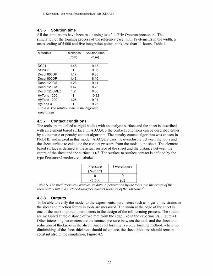
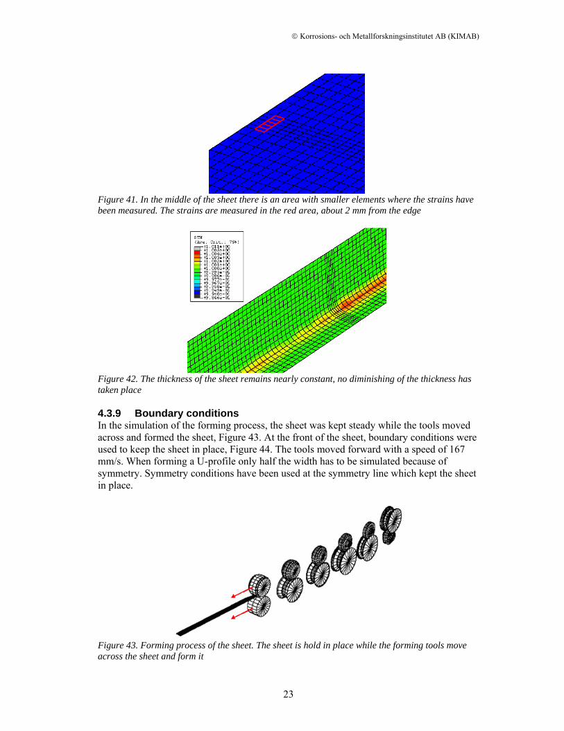
Table 5. The used Pressure-Overclosure data. A penetration by the tools into the centre of the sheet will result in a surface-to-surface contact pressure of 87 500 N/mm2 4.3.8 Outputs To be able to verify the model to the experiments, parameters such as logarithmic strains in the sheet and reaction forces in tools are measured. The strain at the edge of the sheet is one of the most important parameters in the design of the roll forming process. The strains are measured at the distance of two mm from the edge like in the experiments, Figure 41. Other interesting parameters are the contact pressure between the tools and the sheet and reduction of thickness in the sheet. Since roll forming is a pure forming method, where no diminishing of the sheet thickness should take place, the sheet thickness should remain constant also in the simulation, Figure 42.
© Korrosions- och Metallforskningsinstitutet AB (KIMAB)
23
Figure 41. In the middle of the sheet there is an area with smaller elements where the strains have been measured. The strains are measured in the red area, about 2 mm from the edge
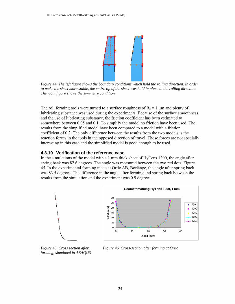
Figure 42. The thickness of the sheet remains nearly constant, no diminishing of the thickness has taken place 4.3.9 Boundary conditions In the simulation of the forming process, the sheet was kept steady while the tools moved across and formed the sheet, Figure 43. At the front of the sheet, boundary conditions were used to keep the sheet in place, Figure 44. The tools moved forward with a speed of 167 mm/s. When forming a U-profile only half the width has to be simulated because of symmetry. Symmetry conditions have been used at the symmetry line which kept the sheet in place.
Figure 43. Forming process of the sheet. The sheet is hold in place while the forming tools move across the sheet and form it
© Korrosions- och Metallforskningsinstitutet AB (KIMAB)
24
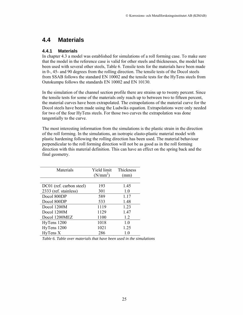
Figure 44. The left figure shows the boundary conditions which hold the rolling direction. In order to make the sheet more stable, the entire tip of the sheet was hold in place in the rolling direction. The right figure shows the symmetry condition The roll forming tools were turned to a surface roughness of Rz = 1 μm and plenty of lubricating substance was used during the experiments. Because of the surface smoothness and the use of lubricating substance, the friction coefficient has been estimated to somewhere between 0.05 and 0.1. To simplify the model no friction have been used. The results from the simplified model have been compared to a model with a friction coefficient of 0.2. The only difference between the results from the two models is the reaction forces in the tools in the opposed direction of travel. Those forces are not specially interesting in this case and the simplified model is good enough to be used. 4.3.10 Verification of the reference case In the simulations of the model with a 1 mm thick sheet of HyTens 1200, the angle after spring back was 82.6 degrees. The angle was measured between the two red dots, Figure 45. In the experimental forming made at Ortic AB, Borlänge, the angle after spring back was 83.5 degrees. The difference in the angle after forming and spring back between the results from the simulation and the experiment was 0.9 degrees.
Geometrimätning HyTens 1200, 1 mm
0
5
10
15
20
25
30
0 10 20 30 40
X-led (mm)
Y-le
d (m
m) 750
1000125015001750
Figure 45. Cross section after forming, simulated in ABAQUS
Figure 46. Cross-section after forming at Ortic
© Korrosions- och Metallforskningsinstitutet AB (KIMAB)
25
4.4 Materials 4.4.1 Materials In chapter 4.3 a model was established for simulations of a roll forming case. To make sure that the model in the reference case is valid for other steels and thicknesses, the model has been used with several other steels, Table 6. Tensile tests for the materials have been made in 0-, 45- and 90 degrees from the rolling direction. The tensile tests of the Docol steels from SSAB follows the standard EN 10002 and the tensile tests for the HyTens steels from Outokumpu follows the standards EN 10002 and EN 10130. In the simulation of the channel section profile there are strains up to twenty percent. Since the tensile tests for some of the materials only reach up to between two to fifteen percent, the material curves have been extrapolated. The extrapolations of the material curve for the Docol steels have been made using the Ludwiks equation. Extrapolations were only needed for two of the four HyTens steels. For those two curves the extrapolation was done tangentially to the curve. The most interesting information from the simulations is the plastic strain in the direction of the roll forming. In the simulations, an isotropic elasto-plastic material model with plastic hardening following the rolling direction has been used. The material behaviour perpendicular to the roll forming direction will not be as good as in the roll forming direction with this material definition. This can have an effect on the spring back and the final geometry.
Materials Yield limit (N/mm2)
Thickness (mm)
DC01 (ref. carbon steel) 193 1.45 2333 (ref. stainless) 301 1.0 Docol 800DP 589 1.17 Docol 800DP 533 1.48 Docol 1200M 1119 1.23 Docol 1200M 1129 1.47 Docol 1200MEZ 1100 1.2 HyTens 1200 1018 1.0 HyTens 1200 1021 1.25 HyTens X 286 1.0
Table 6. Table over materials that have been used in the simulations
© Korrosions- och Metallforskningsinstitutet AB (KIMAB)
26
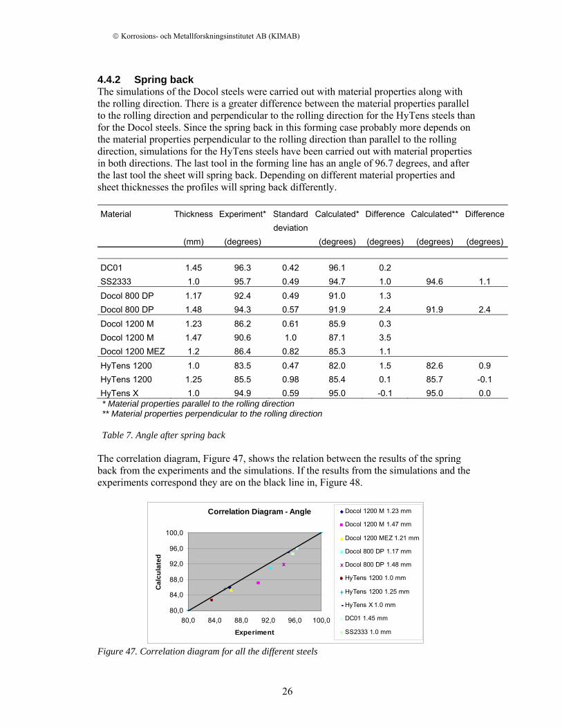
4.4.2 Spring back The simulations of the Docol steels were carried out with material properties along with the rolling direction. There is a greater difference between the material properties parallel to the rolling direction and perpendicular to the rolling direction for the HyTens steels than for the Docol steels. Since the spring back in this forming case probably more depends on the material properties perpendicular to the rolling direction than parallel to the rolling direction, simulations for the HyTens steels have been carried out with material properties in both directions. The last tool in the forming line has an angle of 96.7 degrees, and after the last tool the sheet will spring back. Depending on different material properties and sheet thicknesses the profiles will spring back differently. Material Thickness Experiment* Standard Calculated* Difference Calculated** Difference
deviation (mm) (degrees) (degrees) (degrees) (degrees) (degrees)
DC01 1.45 96.3 0.42 96.1 0.2 SS2333 1.0 95.7 0.49 94.7 1.0 94.6 1.1 Docol 800 DP 1.17 92.4 0.49 91.0 1.3 Docol 800 DP 1.48 94.3 0.57 91.9 2.4 91.9 2.4 Docol 1200 M 1.23 86.2 0.61 85.9 0.3 Docol 1200 M 1.47 90.6 1.0 87.1 3.5 Docol 1200 MEZ 1.2 86.4 0.82 85.3 1.1 HyTens 1200 1.0 83.5 0.47 82.0 1.5 82.6 0.9 HyTens 1200 1.25 85.5 0.98 85.4 0.1 85.7 -0.1 HyTens X 1.0 94.9 0.59 95.0 -0.1 95.0 0.0 * Material properties parallel to the rolling direction ** Material properties perpendicular to the rolling direction Table 7. Angle after spring back
The correlation diagram, Figure 47, shows the relation between the results of the spring back from the experiments and the simulations. If the results from the simulations and the experiments correspond they are on the black line in, Figure 48.
Correlation Diagram - Angle
80,0
84,0
88,0
92,0
96,0
100,0
80,0 84,0 88,0 92,0 96,0 100,0
Experiment
Cal
cula
ted
Docol 1200 M 1.23 mm
Docol 1200 M 1.47 mm
Docol 1200 MEZ 1.21 mm
Docol 800 DP 1.17 mm
Docol 800 DP 1.48 mm
HyTens 1200 1.0 mm
HyTens 1200 1.25 mm
HyTens X 1.0 mm
DC01 1.45 mm
SS2333 1.0 mm
Figure 47. Correlation diagram for all the different steels
© Korrosions- och Metallforskningsinstitutet AB (KIMAB)
27
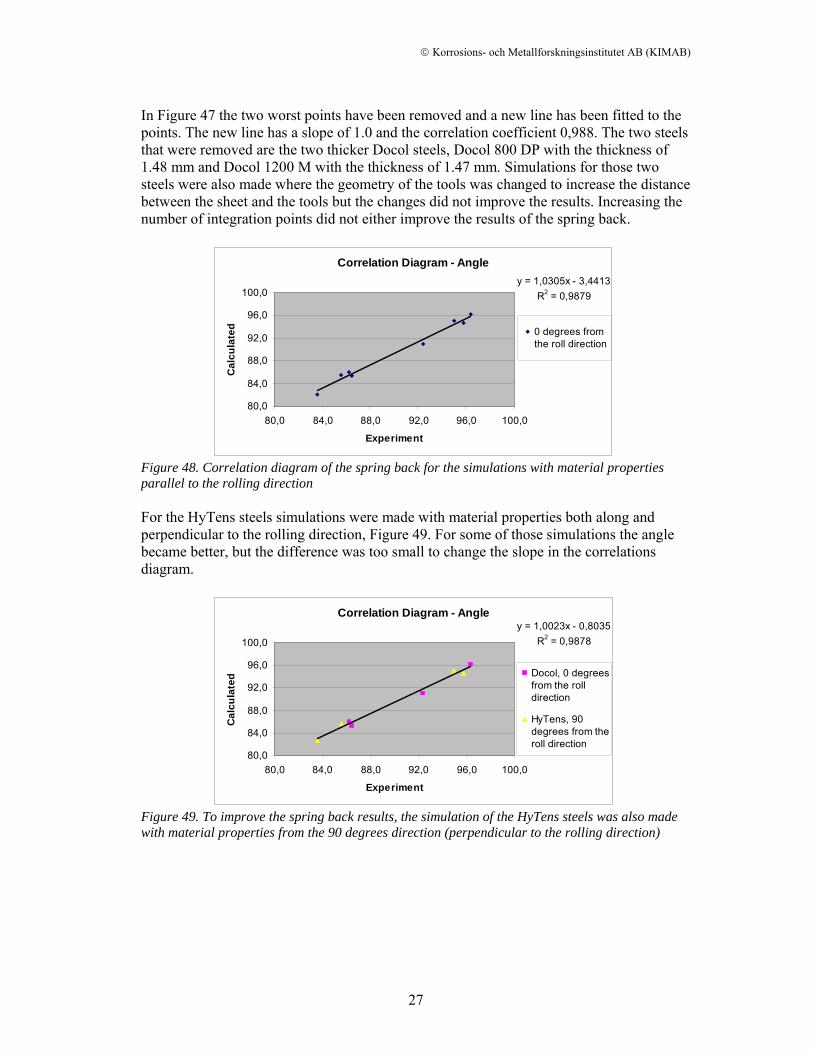
In Figure 47 the two worst points have been removed and a new line has been fitted to the points. The new line has a slope of 1.0 and the correlation coefficient 0,988. The two steels that were removed are the two thicker Docol steels, Docol 800 DP with the thickness of 1.48 mm and Docol 1200 M with the thickness of 1.47 mm. Simulations for those two steels were also made where the geometry of the tools was changed to increase the distance between the sheet and the tools but the changes did not improve the results. Increasing the number of integration points did not either improve the results of the spring back.
Correlation Diagram - Angley = 1,0305x - 3,4413
R2 = 0,9879
80,0
84,0
88,0
92,0
96,0
100,0
80,0 84,0 88,0 92,0 96,0 100,0
Experiment
Cal
cula
ted 0 degrees from
the roll direction
Figure 48. Correlation diagram of the spring back for the simulations with material properties parallel to the rolling direction For the HyTens steels simulations were made with material properties both along and perpendicular to the rolling direction, Figure 49. For some of those simulations the angle became better, but the difference was too small to change the slope in the correlations diagram.
Correlation Diagram - Angley = 1,0023x - 0,8035
R2 = 0,9878
80,0
84,0
88,0
92,0
96,0
100,0
80,0 84,0 88,0 92,0 96,0 100,0
Experiment
Cal
cula
ted Docol, 0 degrees
from the rolldirection
HyTens, 90degrees from theroll direction
Figure 49. To improve the spring back results, the simulation of the HyTens steels was also made with material properties from the 90 degrees direction (perpendicular to the rolling direction)
© Korrosions- och Metallforskningsinstitutet AB (KIMAB)
28
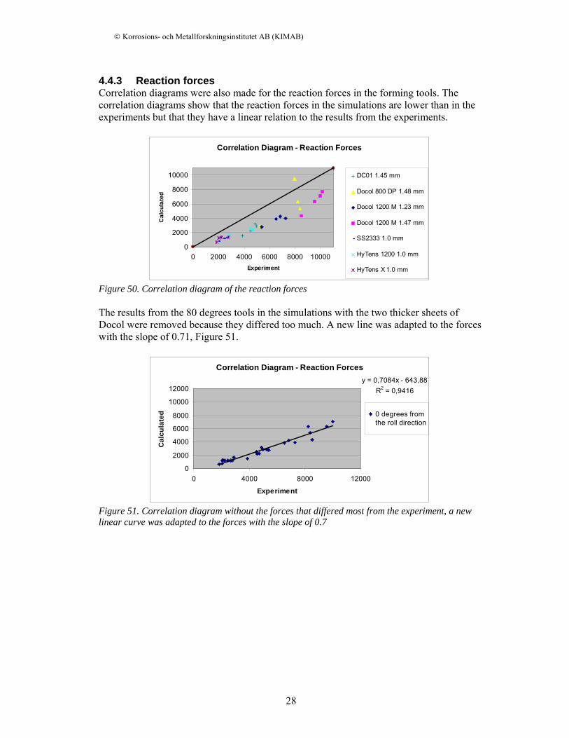
4.4.3 Reaction forces Correlation diagrams were also made for the reaction forces in the forming tools. The correlation diagrams show that the reaction forces in the simulations are lower than in the experiments but that they have a linear relation to the results from the experiments.
Correlation Diagram - Reaction Forces
0
2000
4000
6000
8000
10000
0 2000 4000 6000 8000 10000Experiment
Cal
cula
ted
DC01 1.45 mm
Docol 800 DP 1.48 mm
Docol 1200 M 1.23 mm
Docol 1200 M 1.47 mm
SS2333 1.0 mm
HyTens 1200 1.0 mm
HyTens X 1.0 mm
Figure 50. Correlation diagram of the reaction forces The results from the 80 degrees tools in the simulations with the two thicker sheets of Docol were removed because they differed too much. A new line was adapted to the forces with the slope of 0.71, Figure 51.
Correlation Diagram - Reaction Forcesy = 0,7084x - 643,88
R2 = 0,9416
0
2000
4000
6000
8000
10000
12000
0 4000 8000 12000
Experiment
Cal
cula
ted 0 degrees from
the roll direction
Figure 51. Correlation diagram without the forces that differed most from the experiment, a new linear curve was adapted to the forces with the slope of 0.7
© Korrosions- och Metallforskningsinstitutet AB (KIMAB)
29
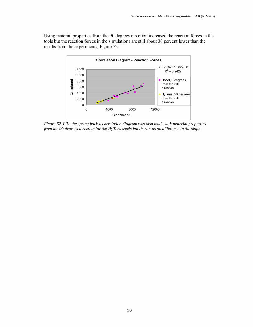
Using material properties from the 90 degrees direction increased the reaction forces in the tools but the reaction forces in the simulations are still about 30 percent lower than the results from the experiments, Figure 52.
Correlation Diagram - Reaction Forces
y = 0,7031x - 590,16R2 = 0,9427
0
2000
4000
6000
8000
10000
12000
0 4000 8000 12000
Experiment
Cal
cula
ted Docol, 0 degrees
from the rolldirection
HyTens, 90 degreesfrom the rolldirection
Figure 52. Like the spring back a correlation diagram was also made with material properties from the 90 degrees direction for the HyTens steels but there was no difference in the slope
© Korrosions- och Metallforskningsinstitutet AB (KIMAB)
30
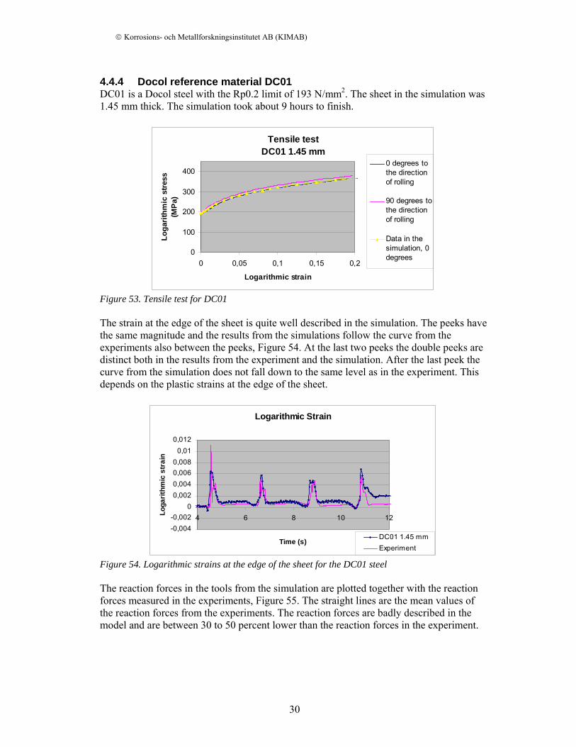
4.4.4 Docol reference material DC01 DC01 is a Docol steel with the Rp0.2 limit of 193 N/mm2. The sheet in the simulation was 1.45 mm thick. The simulation took about 9 hours to finish.
Tensile testDC01 1.45 mm
0
100
200
300
400
0 0,05 0,1 0,15 0,2
Logarithmic strain
Loga
rithm
ic s
tress
(M
Pa)
0 degrees tothe directionof rolling
90 degrees tothe directionof rolling
Data in thesimulation, 0degrees
Figure 53. Tensile test for DC01 The strain at the edge of the sheet is quite well described in the simulation. The peeks have the same magnitude and the results from the simulations follow the curve from the experiments also between the peeks, Figure 54. At the last two peeks the double peeks are distinct both in the results from the experiment and the simulation. After the last peek the curve from the simulation does not fall down to the same level as in the experiment. This depends on the plastic strains at the edge of the sheet.
Logarithmic Strain
-0,004-0,002
00,0020,0040,0060,008
0,010,012
4 6 8 10 12
Time (s)
Loga
rithm
ic s
trai
n
DC01 1.45 mmExperiment
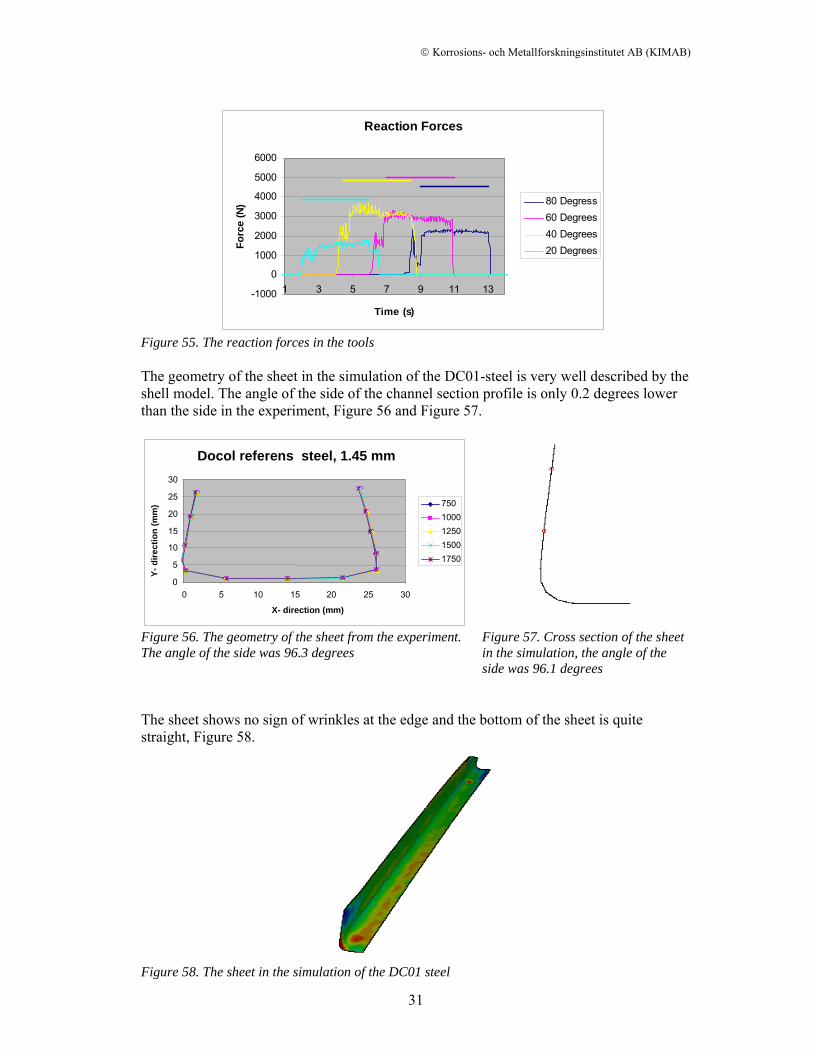
Figure 54. Logarithmic strains at the edge of the sheet for the DC01 steel The reaction forces in the tools from the simulation are plotted together with the reaction forces measured in the experiments, Figure 55. The straight lines are the mean values of the reaction forces from the experiments. The reaction forces are badly described in the model and are between 30 to 50 percent lower than the reaction forces in the experiment.
© Korrosions- och Metallforskningsinstitutet AB (KIMAB)
31
Reaction Forces
-1000
0
1000
2000
3000
4000
5000
6000
1 3 5 7 9 11 13
Time (s)
Forc
e (N
) 80 Degress60 Degrees40 Degrees20 Degrees
Figure 55. The reaction forces in the tools The geometry of the sheet in the simulation of the DC01-steel is very well described by the shell model. The angle of the side of the channel section profile is only 0.2 degrees lower than the side in the experiment, Figure 56 and Figure 57.
Figure 56. The geometry of the sheet from the experiment. The angle of the side was 96.3 degrees
Figure 57. Cross section of the sheet in the simulation, the angle of the side was 96.1 degrees
The sheet shows no sign of wrinkles at the edge and the bottom of the sheet is quite straight, Figure 58.
Figure 58. The sheet in the simulation of the DC01 steel
Docol referens steel, 1.45 mm
0
5
10 15 20 25 30
0 5 10 15 20 25 30
X- direction (mm)
Y- d
irect
ion
(mm
) 7501000125015001750
© Korrosions- och Metallforskningsinstitutet AB (KIMAB)
32
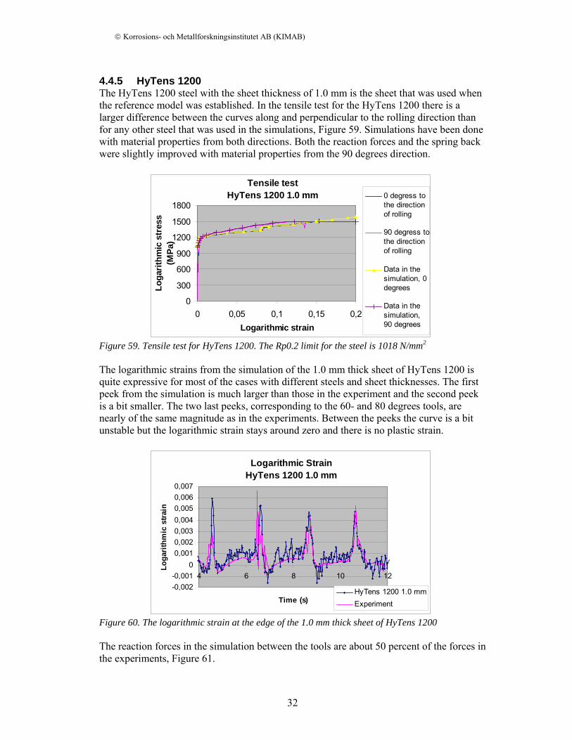
4.4.5 HyTens 1200 The HyTens 1200 steel with the sheet thickness of 1.0 mm is the sheet that was used when the reference model was established. In the tensile test for the HyTens 1200 there is a larger difference between the curves along and perpendicular to the rolling direction than for any other steel that was used in the simulations, Figure 59. Simulations have been done with material properties from both directions. Both the reaction forces and the spring back were slightly improved with material properties from the 90 degrees direction.
Tensile testHyTens 1200 1.0 mm
0
300
600
900
1200
1500
1800
0 0,05 0,1 0,15 0,2Logarithmic strain
Loga
rithm
ic s
tres
s (M
Pa)
0 degress tothe directionof rolling
90 degress tothe directionof rolling
Data in thesimulation, 0degrees
Data in thesimulation,90 degrees
Figure 59. Tensile test for HyTens 1200. The Rp0.2 limit for the steel is 1018 N/mm2 The logarithmic strains from the simulation of the 1.0 mm thick sheet of HyTens 1200 is quite expressive for most of the cases with different steels and sheet thicknesses. The first peek from the simulation is much larger than those in the experiment and the second peek is a bit smaller. The two last peeks, corresponding to the 60- and 80 degrees tools, are nearly of the same magnitude as in the experiments. Between the peeks the curve is a bit unstable but the logarithmic strain stays around zero and there is no plastic strain.
Logarithmic StrainHyTens 1200 1.0 mm
-0,002-0,001
00,0010,0020,0030,0040,0050,0060,007
4 6 8 10 12
Time (s)
Loga
rithm
ic s
train
HyTens 1200 1.0 mmExperiment
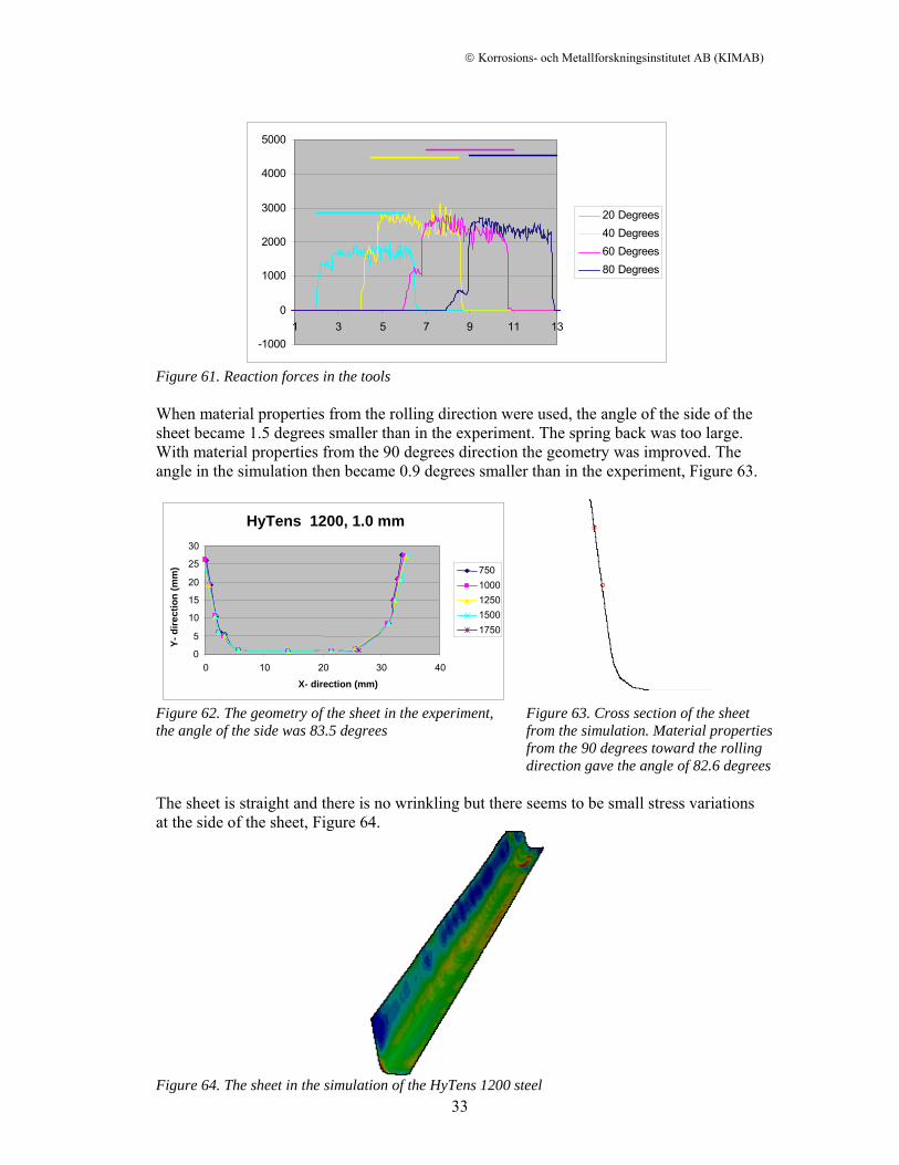
Figure 60. The logarithmic strain at the edge of the 1.0 mm thick sheet of HyTens 1200 The reaction forces in the simulation between the tools are about 50 percent of the forces in the experiments, Figure 61.
© Korrosions- och Metallforskningsinstitutet AB (KIMAB)
33
-1000
0
1000
2000
3000
4000
5000
1 3 5 7 9 11 13
20 Degrees40 Degrees60 Degrees80 Degrees
Figure 61. Reaction forces in the tools When material properties from the rolling direction were used, the angle of the side of the sheet became 1.5 degrees smaller than in the experiment. The spring back was too large. With material properties from the 90 degrees direction the geometry was improved. The angle in the simulation then became 0.9 degrees smaller than in the experiment, Figure 63.
Figure 62. The geometry of the sheet in the experiment, the angle of the side was 83.5 degrees
Figure 63. Cross section of the sheet from the simulation. Material properties from the 90 degrees toward the rolling direction gave the angle of 82.6 degrees
The sheet is straight and there is no wrinkling but there seems to be small stress variations at the side of the sheet, Figure 64.
Figure 64. The sheet in the simulation of the HyTens 1200 steel
HyTens 1200, 1.0 mm
0 5
10 15 20 25 30
0 10 20 30 40
X- direction (mm)
Y- d
irect
ion
(mm
) 7501000125015001750
© Korrosions- och Metallforskningsinstitutet AB (KIMAB)
34
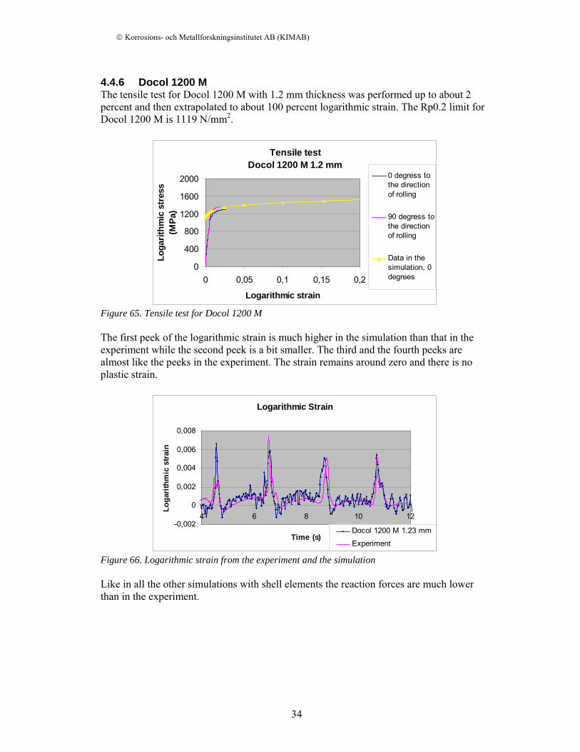
4.4.6 Docol 1200 M The tensile test for Docol 1200 M with 1.2 mm thickness was performed up to about 2 percent and then extrapolated to about 100 percent logarithmic strain. The Rp0.2 limit for Docol 1200 M is 1119 N/mm2.
Tensile testDocol 1200 M 1.2 mm
0
400
800
1200
1600
2000
0 0,05 0,1 0,15 0,2
Logarithmic strain
Loga
rithm
ic s
tres
s (M
Pa)
0 degress tothe directionof rolling
90 degress tothe directionof rolling
Data in thesimulation, 0degrees
Figure 65. Tensile test for Docol 1200 M The first peek of the logarithmic strain is much higher in the simulation than that in the experiment while the second peek is a bit smaller. The third and the fourth peeks are almost like the peeks in the experiment. The strain remains around zero and there is no plastic strain.
Logarithmic Strain
-0,002
0
0,002
0,004
0,006
0,008
4 6 8 10 12
Time (s)
Loga
rithm
ic s
train
Docol 1200 M 1.23 mm
Experiment
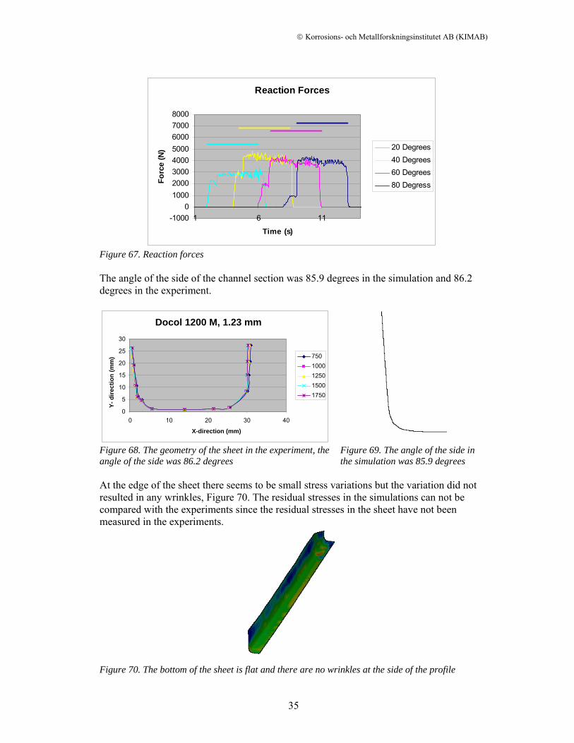
Figure 66. Logarithmic strain from the experiment and the simulation Like in all the other simulations with shell elements the reaction forces are much lower than in the experiment.
© Korrosions- och Metallforskningsinstitutet AB (KIMAB)
35
Reaction Forces
-10000
10002000300040005000600070008000
1 6 11
Time (s)
Forc
e (N
) 20 Degrees40 Degrees60 Degrees80 Degress
Figure 67. Reaction forces The angle of the side of the channel section was 85.9 degrees in the simulation and 86.2 degrees in the experiment.
Figure 68. The geometry of the sheet in the experiment, the angle of the side was 86.2 degrees
Figure 69. The angle of the side in the simulation was 85.9 degrees
At the edge of the sheet there seems to be small stress variations but the variation did not resulted in any wrinkles, Figure 70. The residual stresses in the simulations can not be compared with the experiments since the residual stresses in the sheet have not been measured in the experiments.
Figure 70. The bottom of the sheet is flat and there are no wrinkles at the side of the profile
Docol 1200 M, 1.23 mm
0
5
10 15 20 25 30
0 10 20 30 40
X-direction (mm)
Y- d
irect
ion
(mm
) 7501000125015001750

© Korrosions- och Metallforskningsinstitutet AB (KIMAB)
36
5. Discussion In the model with shell elements both the spring back of the side of the profile and the strains at the edge of the sheet corresponded very well to the experimental result, while the reaction forces in the tools were only half of the reaction forces measured in the experiments. An explanation of the low reaction forces could be that the shell elements do not carry the forces vertical to the plane good enough. In the solid element model with four elements through the thickness the reaction forces were very well described but when the number of elements through the thickness was increased to six elements, the reaction forces increased. Increasing the number of elements through the thickness gave a larger relation between the thickness of the element and the other sides, this might have resulted in an over stiff model. The solid element model did not describe the spring back in a good way. In the reference case, the solid element model showed a spring back nearly twice as high than in the experiment, while the spring back for the shell element model only differed a few percent from the experiment. The effective plastic strain at the bend in the solid element model is about half of the effective plastic strain at the bend in the shell element model, both measured at the bottom surface of the profile. The larger spring back of the solid element model could be caused by the low degree of plasticity. The spring back is generally well predicted for the different steels with the shell element model but in simulations with thicker sheets of high strength steels the spring back has become too large indicating that the model does not describe the behaviour of the thicker sheets accurately. Generally in the simulations, an isotropic elasto-plastic material model with plastic hardening following the rolling direction has been used. The behaviour of the material perpendicular to the roll forming direction will not be described as good as in the roll forming direction with this material definition. This can have an effect on the spring back and the final geometry. To improve the results for the spring back, a material model perpendicular to roll forming direction could be used. In the simulations performed with the implicit solution method none of the simulations was successfully completed. The reason for the failed simulation might be problems in the contact between the sheet and the tools. The implicit solution method is less suited for highly nonlinear problems than the explicit solution method. The simulations, which were performed with the explicit solution method, were accomplished with good results and a solution time within 11 hours. Increasing the number of integration points in the shell element model did not generally improved the spring back. In some simulations the spring back was improved while in some simulations the spring back was unchanged or even deteriorated when the number of integration points was increased from five to nine.

© Korrosions- och Metallforskningsinstitutet AB (KIMAB)
37
6. Conclusion Within this work, simulation of the roll forming of a channel section profile has been performed with several different models. Both implicit and explicit solution methods with both shell and solid elements have been used to optimize the model of the forming process. The results from the simulations have been compared with results from experiments performed by Ortic AB, Borlänge. The final choice of the model:
• The explicit solution method was chosen because no simulation was successfully completed with the implicit solution method.
• Four node shell elements with reduced integration were chosen since the shell
element model described the spring back and the strains at the edge of the sheet much better than the solid element model.
• 18 elements have been used along the width of the sheet. Increasing the number of
elements gave a more instable solution.
• The mass scaling was set to 5000. A higher mass scaling gave a shorter solution time but the solution became more unstable
• The default value of five integration points through the thickness has been used.
Increasing the number of integration points did only improve the results for some of the simulations while the results were unchanged or even deteriorated for the other simulations.
• The sheet length was chosen to 750 mm. In simulations with shorter sheets the
sheets became curved.
• No friction has been used between the sheet and the tools. Results:
• The shell element model gave excellent results of the spring back for the thinner sheets where the results from the simulations were within ±1.5° from experimental results. The spring back for the thicker sheets was slightly overestimated but even so within 3.5°from the experiments.
• The strains at the edge of the sheet were reasonably well described by the model.
The results from the simulations differed a bit from the experiments for the second and the third tool, while the strains in the sheet were very good at the fourth and the fifth tool. The remaining strains at the edge of the sheet were, after spring back, for most of the steels very close to the results in the experiments.
• The reaction forces in the tools were poorly described by the shell element model.
The forces were up to 50 percent lower in the simulations than in the experiments. Even though the reaction forces are too small, the results from the simulations are linearly proportional to the results from the experiments.

© Korrosions- och Metallforskningsinstitutet AB (KIMAB)
38
• There were no wrinkles on the final geometry of the sheet which corresponds to the experimental results.

© Korrosions- och Metallforskningsinstitutet AB (KIMAB)
39
7. Future work In the reference case the explicit solver was chosen since all simulations with the implicit solver failed. Due to the time constraint of this thesis project the further work was concentrated on using the explicit solver. Several of the commercial softwares for simulating roll forming uses the implicit solver. It would be interesting to see how the results and the solution time would be influenced by the different solution methods. The simulations from the solid element model showed very good results for the reaction forces while the geometry of the sheet was poor. Using a solid element model makes it easier to see how the sheet fits and forms between the tools. In the shell element model a penalty contact algorithm was used together with a pressure-overclosure definition to describe the surface-to-surface contact between the tools and the sheet. From the software PROFIL the pressure was chosen to 87 500 N/mm2, when the overclosure between the tools and the sheet was half of the sheet thickness. Further work could be done to see if the reaction forces would be improved if the parameter of 87 500 N/mm2 was changed.

© Korrosions- och Metallforskningsinstitutet AB (KIMAB)
40
8. Acknowledgements This master thesis project has been supervised by Professor Larsgunnar Nilsson, Division of Solid Mechanics, Linköping University. The author would like to thank the members of the project committee for their contribution to this project.
A special thanks to:
Maria Lundberg, Corrosion and Metal Research Institute, for guidance during the project.
Johannes Gårdstam, Corrosion and Metal Research Institute, for help with FE-modelling.
Michael Lindgren, Ortic AB, for all the experimental work.
© Korrosions- och Metallforskningsinstitutet AB (KIMAB)
41
References [1] Formningshandboken (1997) Styckskärande bearbetning och plastisk forming, Utgåva 2, SSAB Tunnplåt, Borlänge [2] ABAQUS version 6.5, Documentation [3] J.C. Nagtegaal, L.M. Taylor (1992) Comparison of Implicit and Explicit Finite Element Methods for Analysis of Sheet Forming Problems - Fundaments of Calculations. Blech Rohre Profile 39, pp. 298-305 [4] Lindgren, M., (2005) Modelling and simulation of the roll forming process, Licentiate Thesis, 2005:40 Luleå University of Technology, Luleå [5] Lindgren, M., (2006a) Formningskraft och Formningsmoment [6] Lindgren, M., (2006b) Formning av profil för mätning i mätmaskin [7] Lundberg, M., (2006) FEM simulation of roll forming - study of the influence of different simulation parameters, IM-2006-126, KIMAB, Stockholm [8] M. Lundberg, L. Gunnarsson, (2006) A benchmark study of available software for design and simulation of roll forming operations, IM-2006-504, KIMAB, Stockholm

© Korrosions- och Metallforskningsinstitutet AB (KIMAB)
42

© Korrosions- och Metallforskningsinstitutet AB (KIMAB)
43
© Korrosions- och Metallforskningsinstitutet AB (KIMAB)
44
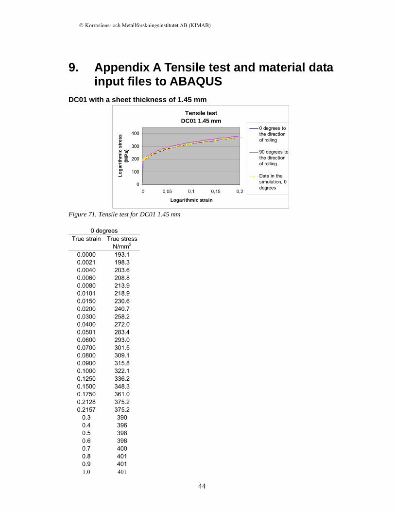
9. Appendix A Tensile test and material data input files to ABAQUS
DC01 with a sheet thickness of 1.45 mm
Tensile testDC01 1.45 mm
0
100
200
300
400
0 0,05 0,1 0,15 0,2
Logarithmic strain
Loga
rith
mic
stre
ss
(MP
a)0 degrees tothe directionof rolling
90 degrees tothe directionof rolling
Data in thesimulation, 0degrees
Figure 71. Tensile test for DC01 1.45 mm
0 degrees True strain True stress
N/mm2 0.0000 193.1 0.0021 198.3 0.0040 203.6 0.0060 208.8 0.0080 213.9 0.0101 218.9 0.0150 230.6 0.0200 240.7 0.0300 258.2 0.0400 272.0 0.0501 283.4 0.0600 293.0 0.0700 301.5 0.0800 309.1 0.0900 315.8 0.1000 322.1 0.1250 336.2 0.1500 348.3 0.1750 361.0 0.2128 375.2 0.2157 375.2
0.3 390 0.4 396 0.5 398 0.6 398 0.7 400 0.8 401 0.9 401 1.0 401
© Korrosions- och Metallforskningsinstitutet AB (KIMAB)
45
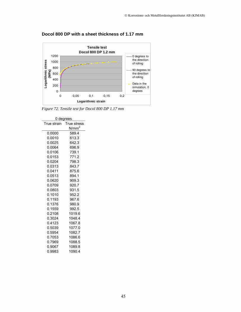
Docol 800 DP with a sheet thickness of 1.17 mm
Tensile testDocol 800 DP 1.2 mm
0
200
400
600
800
1000
1200
0 0,05 0,1 0,15 0,2
Logarithmic strain
Loga
rithm
ic s
tres
s (M
Pa)
0 degress tothe directionof rolling
90 degress tothe directionof rolling
Data in thesimulation, 0degrees
Figure 72. Tensile test for Docol 800 DP 1.17 mm
0 degrees True strain True stress
N/mm2 0.0000 589.4 0.0010 613.3 0.0025 642.3 0.0064 696.9 0.0106 739.1 0.0153 771.2 0.0204 798.3 0.0313 843.7 0.0411 875.6 0.0513 894.1 0.0620 909.3 0.0709 920.7 0.0803 931.5 0.1010 952.2 0.1193 967.6 0.1376 980.9 0.1559 992.5 0.2108 1019.6 0.3024 1048.4 0.4123 1067.8 0.5039 1077.0 0.5954 1082.7 0.7053 1086.6 0.7969 1088.5 0.9067 1089.8 0.9983 1090.4
© Korrosions- och Metallforskningsinstitutet AB (KIMAB)
46
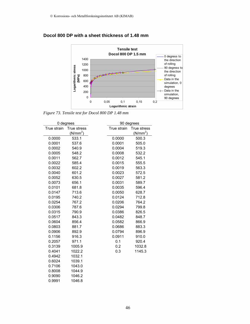
Docol 800 DP with a sheet thickness of 1.48 mm
Tensile testDocol 800 DP 1.5 mm
0
200
400
600
800
1000
1200
1400
0 0,05 0,1 0,15 0,2Logarithmic strain
Loga
rithm
ic s
tress
(M
Pa)
0 degress tothe directionof rolling90 degress tothe directionof rollingData in thesimulation, 0degreesData in thesimulation,90 degrees
Figure 73. Tensile test for Docol 800 DP 1.48 mm
0 degrees 90 degrees True strain True stress True strain True stress
(N/mm2) (N/mm2) 0.0000 533.1 0.0000 500.3 0.0001 537.6 0.0001 505.0 0.0002 540.9 0.0004 519.3 0.0005 548.2 0.0008 532.2 0.0011 562.7 0.0012 545.1 0.0022 585.4 0.0015 555.5 0.0032 602.2 0.0019 563.3 0.0040 601.2 0.0023 572.5 0.0052 630.5 0.0027 581.2 0.0073 656.1 0.0031 589.7 0.0101 681.8 0.0035 596.4 0.0147 713.6 0.0050 628.7 0.0195 740.2 0.0124 712.8 0.0254 767.2 0.0206 764.2 0.0306 787.6 0.0294 799.8 0.0315 790.9 0.0386 826.5 0.0517 843.3 0.0482 848.7 0.0604 856.4 0.0582 866.9 0.0803 881.7 0.0686 883.3 0.0906 892.9 0.0794 896.9 0.1156 916.3 0.0911 910.0 0.2057 971.1 0.1 920.4 0.3139 1005.9 0.2 1032.8 0.4041 1022.2 0.3 1145.3 0.4942 1032.1 0.6024 1039.1 0.7106 1043.0 0.8008 1044.9 0.9090 1046.2 0.9991 1046.8
© Korrosions- och Metallforskningsinstitutet AB (KIMAB)
47
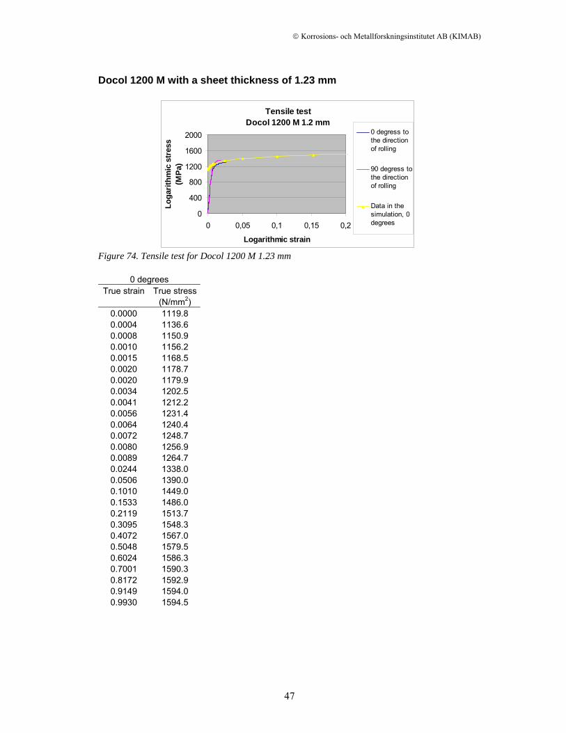
Docol 1200 M with a sheet thickness of 1.23 mm
Tensile testDocol 1200 M 1.2 mm
0
400
800
1200
1600
2000
0 0,05 0,1 0,15 0,2
Logarithmic strain
Loga
rithm
ic s
tres
s (M
Pa)
0 degress tothe directionof rolling
90 degress tothe directionof rolling
Data in thesimulation, 0degrees
Figure 74. Tensile test for Docol 1200 M 1.23 mm
0 degrees True strain True stress
(N/mm2) 0.0000 1119.8 0.0004 1136.6 0.0008 1150.9 0.0010 1156.2 0.0015 1168.5 0.0020 1178.7 0.0020 1179.9 0.0034 1202.5 0.0041 1212.2 0.0056 1231.4 0.0064 1240.4 0.0072 1248.7 0.0080 1256.9 0.0089 1264.7 0.0244 1338.0 0.0506 1390.0 0.1010 1449.0 0.1533 1486.0 0.2119 1513.7 0.3095 1548.3 0.4072 1567.0 0.5048 1579.5 0.6024 1586.3 0.7001 1590.3 0.8172 1592.9 0.9149 1594.0 0.9930 1594.5
© Korrosions- och Metallforskningsinstitutet AB (KIMAB)
48
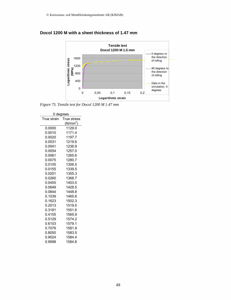
Docol 1200 M with a sheet thickness of 1.47 mm
Tensile testDocol 1200 M 1.5 mm
0
400
800
1200
1600
0 0,05 0,1 0,15 0,2
Logarithmic strain
Loga
rithm
ic s
tres
s (M
Pa)
0 degress tothe directionof rolling
90 degress tothe directionof rolling
Data in thesimulation, 0degrees
Figure 75. Tensile test for Docol 1200 M 1.47 mm
0 degrees True strain True stress
(N/mm2) 0.0000 1129.0 0.0010 1171.4 0.0020 1197.7 0.0031 1219.6 0.0041 1236.9 0.0054 1257.0 0.0061 1265.6 0.0075 1280.7 0.0105 1306.5 0.0155 1339.5 0.0201 1355.3 0.0260 1368.7 0.0455 1403.0 0.0649 1428.5 0.0844 1448.8 0.1039 1465.6 0.1623 1502.3 0.2013 1519.5 0.3181 1551.6 0.4155 1565.9 0.5129 1574.2 0.6103 1579.1 0.7076 1581.9 0.8050 1583.5 0.9024 1584.4 0.9998 1584.8
© Korrosions- och Metallforskningsinstitutet AB (KIMAB)
49
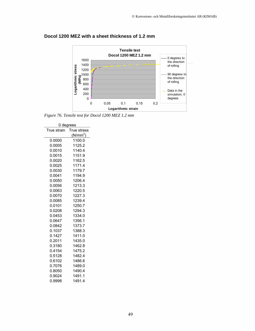
Docol 1200 MEZ with a sheet thickness of 1.2 mm
Tensile testDocol 1200 MEZ 1.2 mm
0200400600800
1000120014001600
0 0,05 0,1 0,15 0,2Logarithmic strain
Loga
rithm
ic s
tres
s (M
Pa)
0 degress tothe directionof rolling
90 degress tothe directionof rolling
Data in thesimulation, 0degrees
Figure 76. Tensile test for Docol 1200 MEZ 1.2 mm
0 degrees True strain True stress
(N/mm2) 0.0000 1100.0 0.0005 1125.2 0.0010 1140.4 0.0015 1151.9 0.0020 1162.5 0.0025 1171.4 0.0030 1179.7 0.0041 1194.9 0.0050 1206.4 0.0056 1213.3 0.0063 1220.5 0.0070 1227.3 0.0085 1239.4 0.0101 1250.7 0.0208 1294.3 0.0453 1334.0 0.0647 1356.1 0.0842 1373.7 0.1037 1388.3 0.1427 1411.0 0.2011 1435.0 0.3180 1462.8 0.4154 1475.2 0.5128 1482.4 0.6102 1486.6 0.7076 1489.0 0.8050 1490.4 0.9024 1491.1 0.9998 1491.4
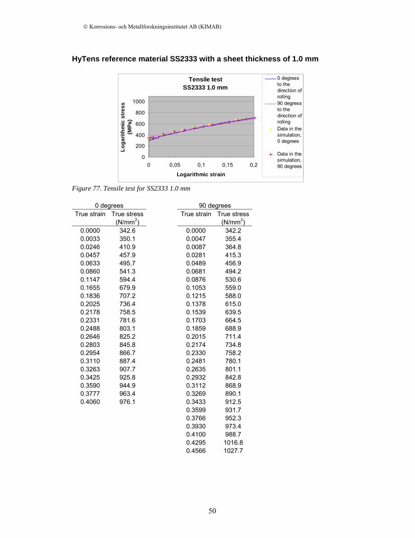
© Korrosions- och Metallforskningsinstitutet AB (KIMAB)
50
HyTens reference material SS2333 with a sheet thickness of 1.0 mm
Tensile testSS2333 1.0 mm
0
200
400
600
800
1000
0 0,05 0,1 0,15 0,2
Logarithmic strain
Loga
rithm
ic s
tres
s (M
Pa)
0 degressto thedirection ofrolling90 degressto thedirection ofrollingData in thesimulation,0 degrees
Data in thesimulation,90 degrees
Figure 77. Tensile test for SS2333 1.0 mm
0 degrees 90 degrees True strain True stress True strain True stress
(N/mm2) (N/mm2) 0.0000 342.6 0.0000 342.2 0.0033 350.1 0.0047 355.4 0.0246 410.9 0.0087 364.8 0.0457 457.9 0.0281 415.3 0.0633 495.7 0.0489 456.9 0.0860 541.3 0.0681 494.2 0.1147 594.4 0.0876 530.6 0.1655 679.9 0.1053 559.0 0.1836 707.2 0.1215 588.0 0.2025 736.4 0.1378 615.0 0.2178 758.5 0.1539 639.5 0.2331 781.6 0.1703 664.5 0.2488 803.1 0.1859 688.9 0.2646 825.2 0.2015 711.4 0.2803 845.8 0.2174 734.8 0.2954 866.7 0.2330 758.2 0.3110 887.4 0.2481 780.1 0.3263 907.7 0.2635 801.1 0.3425 925.8 0.2932 842.8 0.3590 944.9 0.3112 868.9 0.3777 963.4 0.3269 890.1 0.4060 976.1 0.3433 912.5
0.3599 931.7 0.3766 952.3 0.3930 973.4 0.4100 988.7 0.4295 1016.8 0.4566 1027.7
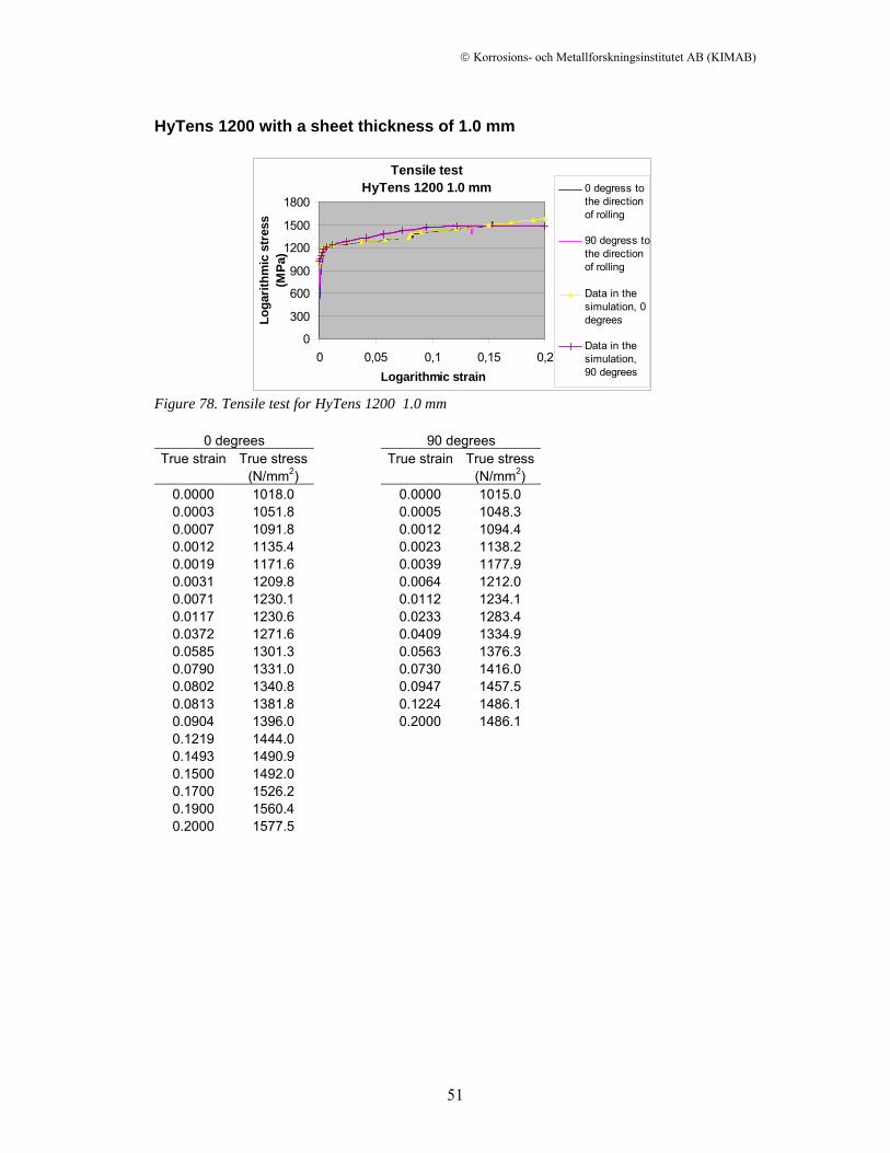
© Korrosions- och Metallforskningsinstitutet AB (KIMAB)
51
HyTens 1200 with a sheet thickness of 1.0 mm
Tensile testHyTens 1200 1.0 mm
0
300
600
900
1200
1500
1800
0 0,05 0,1 0,15 0,2Logarithmic strain
Loga
rithm
ic s
tres
s (M
Pa)
0 degress tothe directionof rolling
90 degress tothe directionof rolling
Data in thesimulation, 0degrees
Data in thesimulation,90 degrees
Figure 78. Tensile test for HyTens 1200 1.0 mm
0 degrees 90 degrees True strain True stress True strain True stress
(N/mm2) (N/mm2) 0.0000 1018.0 0.0000 1015.0 0.0003 1051.8 0.0005 1048.3 0.0007 1091.8 0.0012 1094.4 0.0012 1135.4 0.0023 1138.2 0.0019 1171.6 0.0039 1177.9 0.0031 1209.8 0.0064 1212.0 0.0071 1230.1 0.0112 1234.1 0.0117 1230.6 0.0233 1283.4 0.0372 1271.6 0.0409 1334.9 0.0585 1301.3 0.0563 1376.3 0.0790 1331.0 0.0730 1416.0 0.0802 1340.8 0.0947 1457.5 0.0813 1381.8 0.1224 1486.1 0.0904 1396.0 0.2000 1486.1 0.1219 1444.0 0.1493 1490.9 0.1500 1492.0 0.1700 1526.2 0.1900 1560.4 0.2000 1577.5
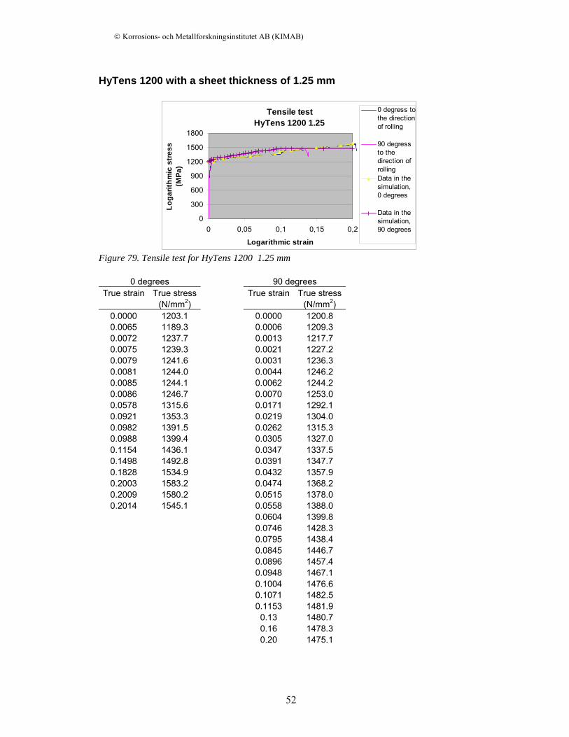
© Korrosions- och Metallforskningsinstitutet AB (KIMAB)
52
HyTens 1200 with a sheet thickness of 1.25 mm
Tensile testHyTens 1200 1.25
0
300
600
900
1200
1500
1800
0 0,05 0,1 0,15 0,2
Logarithmic strain
Loga
rithm
ic s
tres
s (M
Pa)
0 degress tothe directionof rolling
90 degressto thedirection ofrollingData in thesimulation,0 degrees
Data in thesimulation,90 degrees
Figure 79. Tensile test for HyTens 1200 1.25 mm
0 degrees 90 degrees True strain True stress True strain True stress
(N/mm2) (N/mm2) 0.0000 1203.1 0.0000 1200.8 0.0065 1189.3 0.0006 1209.3 0.0072 1237.7 0.0013 1217.7 0.0075 1239.3 0.0021 1227.2 0.0079 1241.6 0.0031 1236.3 0.0081 1244.0 0.0044 1246.2 0.0085 1244.1 0.0062 1244.2 0.0086 1246.7 0.0070 1253.0 0.0578 1315.6 0.0171 1292.1 0.0921 1353.3 0.0219 1304.0 0.0982 1391.5 0.0262 1315.3 0.0988 1399.4 0.0305 1327.0 0.1154 1436.1 0.0347 1337.5 0.1498 1492.8 0.0391 1347.7 0.1828 1534.9 0.0432 1357.9 0.2003 1583.2 0.0474 1368.2 0.2009 1580.2 0.0515 1378.0 0.2014 1545.1 0.0558 1388.0
0.0604 1399.8 0.0746 1428.3 0.0795 1438.4 0.0845 1446.7 0.0896 1457.4 0.0948 1467.1 0.1004 1476.6 0.1071 1482.5 0.1153 1481.9 0.13 1480.7 0.16 1478.3 0.20 1475.1
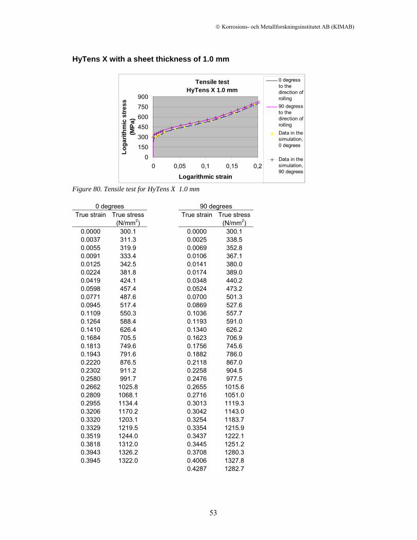
© Korrosions- och Metallforskningsinstitutet AB (KIMAB)
53
HyTens X with a sheet thickness of 1.0 mm
Tensile testHyTens X 1.0 mm
0150300450600750900
0 0,05 0,1 0,15 0,2
Logarithmic strain
Loga
rithm
ic s
tress
(M
Pa)
0 degressto thedirection ofrolling90 degressto thedirection ofrollingData in thesimulation,0 degrees
Data in thesimulation,90 degrees
Figure 80. Tensile test for HyTens X 1.0 mm
0 degrees 90 degrees True strain True stress True strain True stress
(N/mm2) (N/mm2) 0.0000 300.1 0.0000 300.1 0.0037 311.3 0.0025 338.5 0.0055 319.9 0.0069 352.8 0.0091 333.4 0.0106 367.1 0.0125 342.5 0.0141 380.0 0.0224 381.8 0.0174 389.0 0.0419 424.1 0.0348 440.2 0.0598 457.4 0.0524 473.2 0.0771 487.6 0.0700 501.3 0.0945 517.4 0.0869 527.6 0.1109 550.3 0.1036 557.7 0.1264 588.4 0.1193 591.0 0.1410 626.4 0.1340 626.2 0.1684 705.5 0.1623 706.9 0.1813 749.6 0.1756 745.6 0.1943 791.6 0.1882 786.0 0.2220 876.5 0.2118 867.0 0.2302 911.2 0.2258 904.5 0.2580 991.7 0.2476 977.5 0.2662 1025.8 0.2655 1015.6 0.2809 1068.1 0.2716 1051.0 0.2955 1134.4 0.3013 1119.3 0.3206 1170.2 0.3042 1143.0 0.3320 1203.1 0.3254 1183.7 0.3329 1219.5 0.3354 1215.9 0.3519 1244.0 0.3437 1222.1 0.3818 1312.0 0.3445 1251.2 0.3943 1326.2 0.3708 1280.3 0.3945 1322.0 0.4006 1327.8
0.4287 1282.7
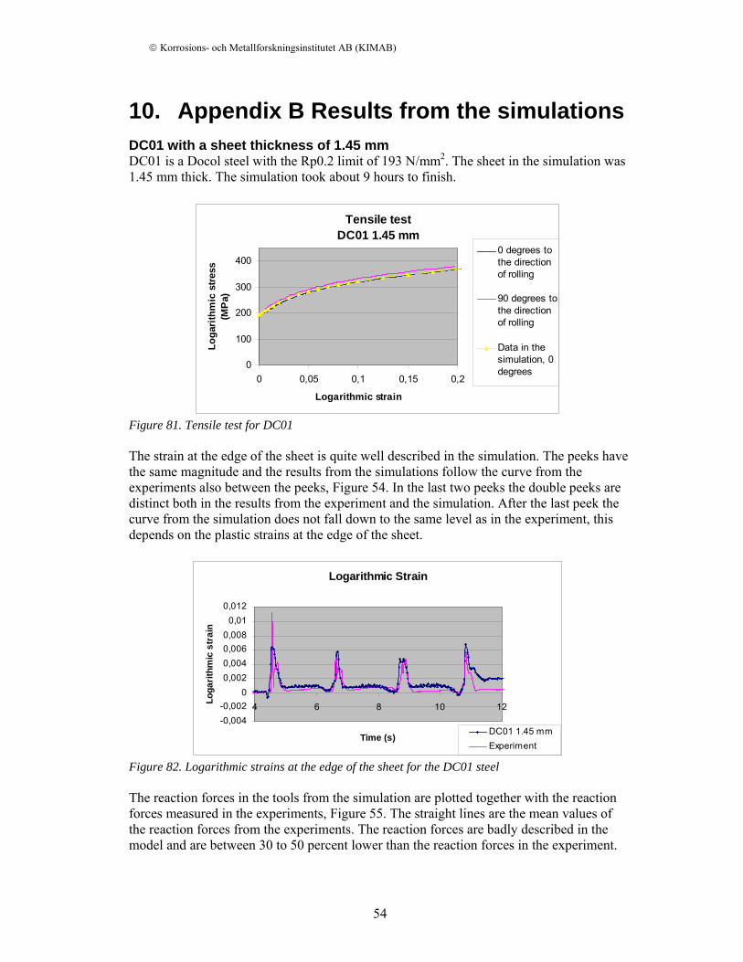
© Korrosions- och Metallforskningsinstitutet AB (KIMAB)
54
10. Appendix B Results from the simulations DC01 with a sheet thickness of 1.45 mm DC01 is a Docol steel with the Rp0.2 limit of 193 N/mm2. The sheet in the simulation was 1.45 mm thick. The simulation took about 9 hours to finish.
Tensile testDC01 1.45 mm
0
100
200
300
400
0 0,05 0,1 0,15 0,2
Logarithmic strain
Loga
rithm
ic s
tress
(M
Pa)
0 degrees tothe directionof rolling
90 degrees tothe directionof rolling
Data in thesimulation, 0degrees
Figure 81. Tensile test for DC01 The strain at the edge of the sheet is quite well described in the simulation. The peeks have the same magnitude and the results from the simulations follow the curve from the experiments also between the peeks, Figure 54. In the last two peeks the double peeks are distinct both in the results from the experiment and the simulation. After the last peek the curve from the simulation does not fall down to the same level as in the experiment, this depends on the plastic strains at the edge of the sheet.
Logarithmic Strain
-0,004-0,002
00,0020,0040,0060,008
0,010,012
4 6 8 10 12
Time (s)
Loga
rithm
ic s
trai
n
DC01 1.45 mmExperiment
Figure 82. Logarithmic strains at the edge of the sheet for the DC01 steel The reaction forces in the tools from the simulation are plotted together with the reaction forces measured in the experiments, Figure 55. The straight lines are the mean values of the reaction forces from the experiments. The reaction forces are badly described in the model and are between 30 to 50 percent lower than the reaction forces in the experiment.
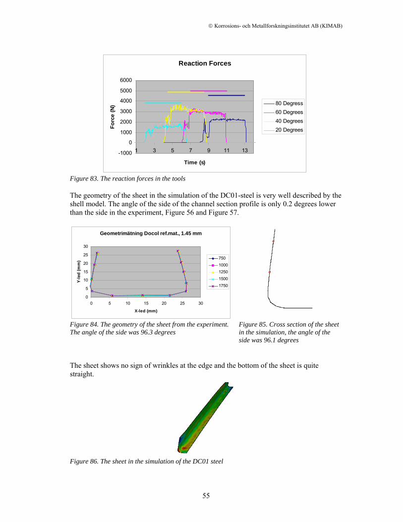
© Korrosions- och Metallforskningsinstitutet AB (KIMAB)
55
Reaction Forces
-1000
0
1000
2000
3000
4000
5000
6000
1 3 5 7 9 11 13
Time (s)
Forc
e (N
) 80 Degress60 Degrees40 Degrees20 Degrees
Figure 83. The reaction forces in the tools The geometry of the sheet in the simulation of the DC01-steel is very well described by the shell model. The angle of the side of the channel section profile is only 0.2 degrees lower than the side in the experiment, Figure 56 and Figure 57.
Geometrimätning Docol ref.mat., 1.45 mm
0
5
10
15
20
25
30
0 5 10 15 20 25 30
X-led (mm)
Y-le
d (m
m) 750
1000125015001750
Figure 84. The geometry of the sheet from the experiment. The angle of the side was 96.3 degrees
Figure 85. Cross section of the sheet in the simulation, the angle of the side was 96.1 degrees
The sheet shows no sign of wrinkles at the edge and the bottom of the sheet is quite straight.
Figure 86. The sheet in the simulation of the DC01 steel
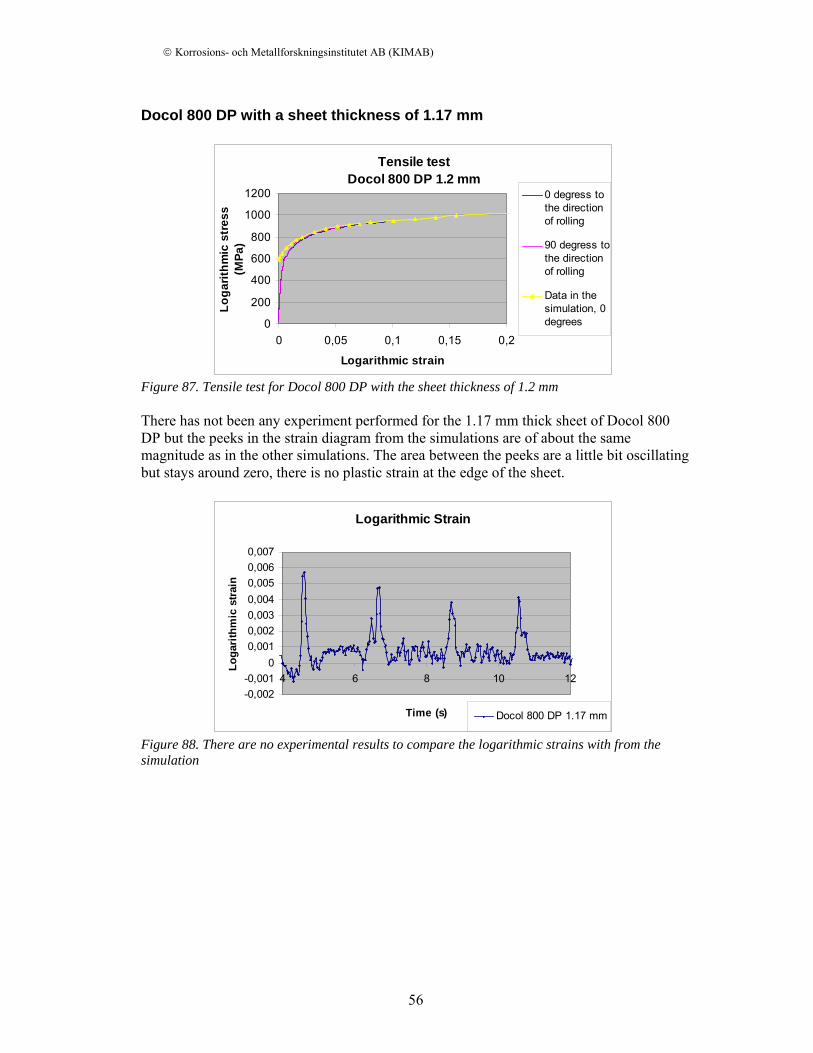
© Korrosions- och Metallforskningsinstitutet AB (KIMAB)
56
Docol 800 DP with a sheet thickness of 1.17 mm
Tensile testDocol 800 DP 1.2 mm
0
200
400
600
800
1000
1200
0 0,05 0,1 0,15 0,2
Logarithmic strain
Loga
rithm
ic s
tres
s (M
Pa)
0 degress tothe directionof rolling
90 degress tothe directionof rolling
Data in thesimulation, 0degrees
Figure 87. Tensile test for Docol 800 DP with the sheet thickness of 1.2 mm There has not been any experiment performed for the 1.17 mm thick sheet of Docol 800 DP but the peeks in the strain diagram from the simulations are of about the same magnitude as in the other simulations. The area between the peeks are a little bit oscillating but stays around zero, there is no plastic strain at the edge of the sheet.
Logarithmic Strain
-0,002-0,001
00,0010,0020,0030,0040,0050,0060,007
4 6 8 10 12
Time (s)
Loga
rithm
ic s
train
Docol 800 DP 1.17 mm
Figure 88. There are no experimental results to compare the logarithmic strains with from the simulation
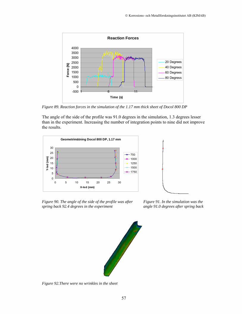
© Korrosions- och Metallforskningsinstitutet AB (KIMAB)
57
Reaction Forces
-5000
5001000150020002500300035004000
1 6 11
Time (s)
Forc
e (N
) 20 Degrees40 Degrees60 Degrees80 Degress
Figure 89. Reaction forces in the simulation of the 1.17 mm thick sheet of Docol 800 DP The angle of the side of the profile was 91.0 degrees in the simulation, 1.3 degrees lesser than in the experiment. Increasing the number of integration points to nine did not improve the results.
Geometrimätning Docol 800 DP, 1.17 mm
0
5
10
15
20
25
30
0 5 10 15 20 25 30
X-led (mm)
Y-le
d (m
m) 750
1000125015001750
Figure 90. The angle of the side of the profile was after spring back 92.4 degrees in the experiment
Figure 91. In the simulation was the angle 91.0 degrees after spring back
Figure 92.There were no wrinkles in the sheet
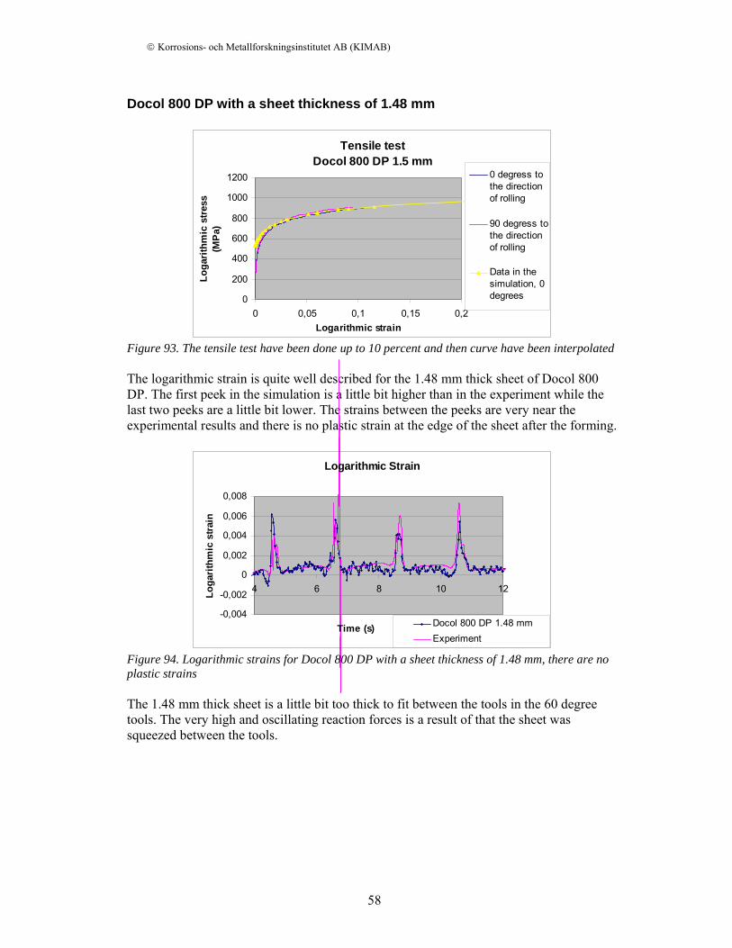
© Korrosions- och Metallforskningsinstitutet AB (KIMAB)
58
Docol 800 DP with a sheet thickness of 1.48 mm
Tensile testDocol 800 DP 1.5 mm
0
200
400
600
800
1000
1200
0 0,05 0,1 0,15 0,2Logarithmic strain
Loga
rithm
ic s
tress
(M
Pa)
0 degress tothe directionof rolling
90 degress tothe directionof rolling
Data in thesimulation, 0degrees
Figure 93. The tensile test have been done up to 10 percent and then curve have been interpolated The logarithmic strain is quite well described for the 1.48 mm thick sheet of Docol 800 DP. The first peek in the simulation is a little bit higher than in the experiment while the last two peeks are a little bit lower. The strains between the peeks are very near the experimental results and there is no plastic strain at the edge of the sheet after the forming.
Logarithmic Strain
-0,004
-0,002
0
0,002
0,004
0,006
0,008
4 6 8 10 12
Time (s)
Loga
rithm
ic s
train
Docol 800 DP 1.48 mmExperiment
Figure 94. Logarithmic strains for Docol 800 DP with a sheet thickness of 1.48 mm, there are no plastic strains The 1.48 mm thick sheet is a little bit too thick to fit between the tools in the 60 degree tools. The very high and oscillating reaction forces is a result of that the sheet was squeezed between the tools.
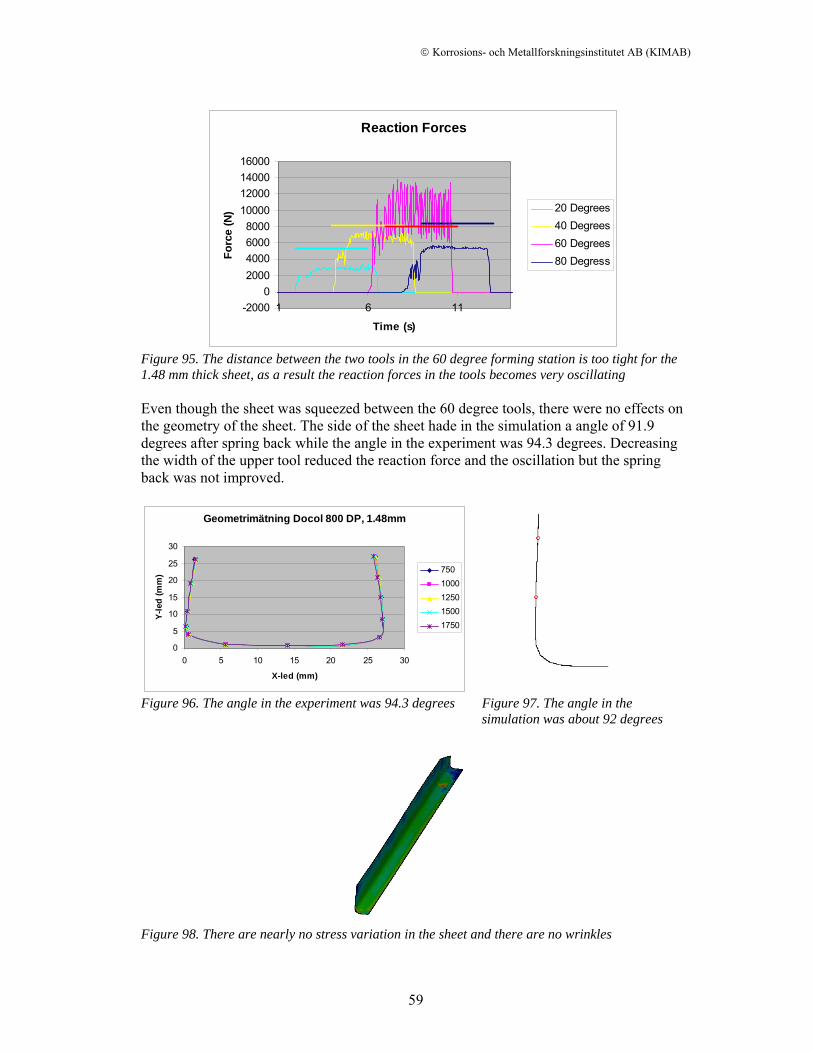
© Korrosions- och Metallforskningsinstitutet AB (KIMAB)
59
Reaction Forces
-20000
2000400060008000
10000120001400016000
1 6 11
Time (s)
Forc
e (N
) 20 Degrees40 Degrees60 Degrees80 Degress
Figure 95. The distance between the two tools in the 60 degree forming station is too tight for the 1.48 mm thick sheet, as a result the reaction forces in the tools becomes very oscillating Even though the sheet was squeezed between the 60 degree tools, there were no effects on the geometry of the sheet. The side of the sheet hade in the simulation a angle of 91.9 degrees after spring back while the angle in the experiment was 94.3 degrees. Decreasing the width of the upper tool reduced the reaction force and the oscillation but the spring back was not improved.
Geometrimätning Docol 800 DP, 1.48mm
0
5
10
15
20
25
30
0 5 10 15 20 25 30
X-led (mm)
Y-le
d (m
m) 750
1000125015001750
Figure 96. The angle in the experiment was 94.3 degrees Figure 97. The angle in the simulation was about 92 degrees
Figure 98. There are nearly no stress variation in the sheet and there are no wrinkles
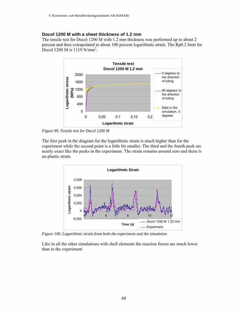
© Korrosions- och Metallforskningsinstitutet AB (KIMAB)
60
Docol 1200 M with a sheet thickness of 1.2 mm The tensile test for Docol 1200 M with 1.2 mm thickness was performed up to about 2 percent and then extrapolated to about 100 percent logarithmic strain. The Rp0.2 limit for Docol 1200 M is 1119 N/mm2.
Tensile testDocol 1200 M 1.2 mm
0
400
800
1200
1600
2000
0 0,05 0,1 0,15 0,2
Logarithmic strain
Loga
rithm
ic s
tres
s (M
Pa)
0 degress tothe directionof rolling
90 degress tothe directionof rolling
Data in thesimulation, 0degrees
Figure 99. Tensile test for Docol 1200 M The first peek in the diagram for the logarithmic strain is much higher than for the experiment while the second point is a little bit smaller. The third and the fourth peek are nearly exact like the peeks in the experiment. The strain remains around zero and there is no plastic strain.
Logarithmic Strain
-0,002
0
0,002
0,004
0,006
0,008
4 6 8 10 12
Time (s)
Loga
rithm
ic s
train
Docol 1200 M 1.23 mm
Experiment
Figure 100. Logarithmic strain from both the experiment and the simulation Like in all the other simulations with shell elements the reaction forces are much lower than in the experiment.
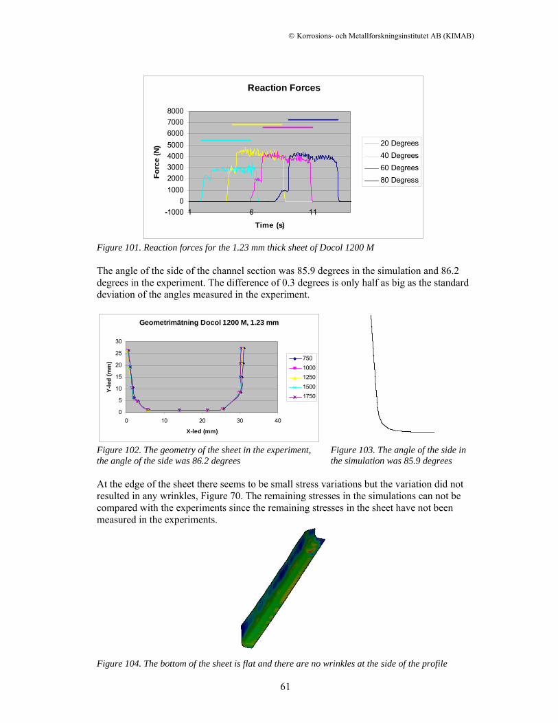
© Korrosions- och Metallforskningsinstitutet AB (KIMAB)
61
Reaction Forces
-10000
10002000300040005000600070008000
1 6 11
Time (s)
Forc
e (N
) 20 Degrees40 Degrees60 Degrees80 Degress
Figure 101. Reaction forces for the 1.23 mm thick sheet of Docol 1200 M The angle of the side of the channel section was 85.9 degrees in the simulation and 86.2 degrees in the experiment. The difference of 0.3 degrees is only half as big as the standard deviation of the angles measured in the experiment.
Geometrimätning Docol 1200 M, 1.23 mm
0
5
10
15
20
25
30
0 10 20 30 40
X-led (mm)
Y-le
d (m
m) 750
1000125015001750
Figure 102. The geometry of the sheet in the experiment, the angle of the side was 86.2 degrees
Figure 103. The angle of the side in the simulation was 85.9 degrees
At the edge of the sheet there seems to be small stress variations but the variation did not resulted in any wrinkles, Figure 70. The remaining stresses in the simulations can not be compared with the experiments since the remaining stresses in the sheet have not been measured in the experiments.
Figure 104. The bottom of the sheet is flat and there are no wrinkles at the side of the profile
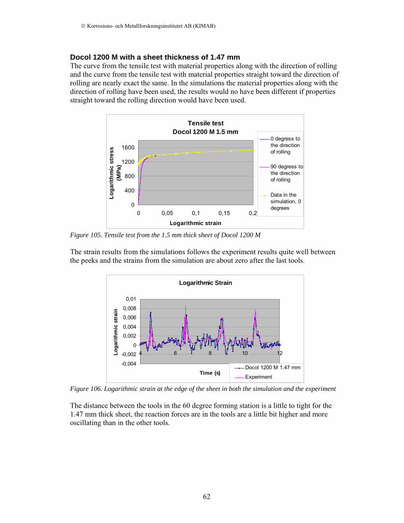
© Korrosions- och Metallforskningsinstitutet AB (KIMAB)
62
Docol 1200 M with a sheet thickness of 1.47 mm The curve from the tensile test with material properties along with the direction of rolling and the curve from the tensile test with material properties straight toward the direction of rolling are nearly exact the same. In the simulations the material properties along with the direction of rolling have been used, the results would no have been different if properties straight toward the rolling direction would have been used.
Tensile testDocol 1200 M 1.5 mm
0
400
800
1200
1600
0 0,05 0,1 0,15 0,2
Logarithmic strain
Loga
rithm
ic s
tres
s (M
Pa)
0 degress tothe directionof rolling
90 degress tothe directionof rolling
Data in thesimulation, 0degrees
Figure 105. Tensile test from the 1.5 mm thick sheet of Docol 1200 M The strain results from the simulations follows the experiment results quite well between the peeks and the strains from the simulation are about zero after the last tools.
Logarithmic Strain
-0,004
-0,002
0
0,002
0,004
0,006
0,008
0,01
4 6 8 10 12
Time (s)
Loga
rithm
ic s
train
Docol 1200 M 1.47 mm
Experiment
Figure 106. Logarithmic strain at the edge of the sheet in both the simulation and the experiment The distance between the tools in the 60 degree forming station is a little to tight for the 1.47 mm thick sheet, the reaction forces are in the tools are a little bit higher and more oscillating than in the other tools.
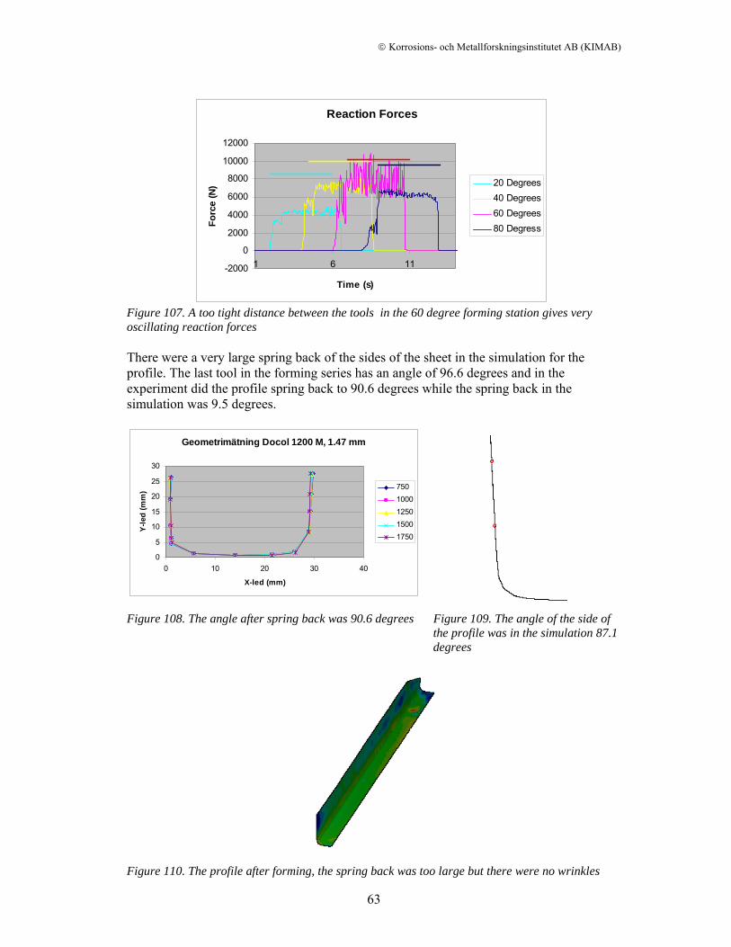
© Korrosions- och Metallforskningsinstitutet AB (KIMAB)
63
Reaction Forces
-2000
0
2000
4000
6000
8000
10000
12000
1 6 11
Time (s)
Forc
e (N
) 20 Degrees40 Degrees60 Degrees80 Degress
Figure 107. A too tight distance between the tools in the 60 degree forming station gives very oscillating reaction forces There were a very large spring back of the sides of the sheet in the simulation for the profile. The last tool in the forming series has an angle of 96.6 degrees and in the experiment did the profile spring back to 90.6 degrees while the spring back in the simulation was 9.5 degrees.
Geometrimätning Docol 1200 M, 1.47 mm
0
5
10
15
20
25
30
0 10 20 30 40
X-led (mm)
Y-le
d (m
m) 750
1000125015001750
Figure 108. The angle after spring back was 90.6 degrees Figure 109. The angle of the side of
the profile was in the simulation 87.1 degrees
Figure 110. The profile after forming, the spring back was too large but there were no wrinkles
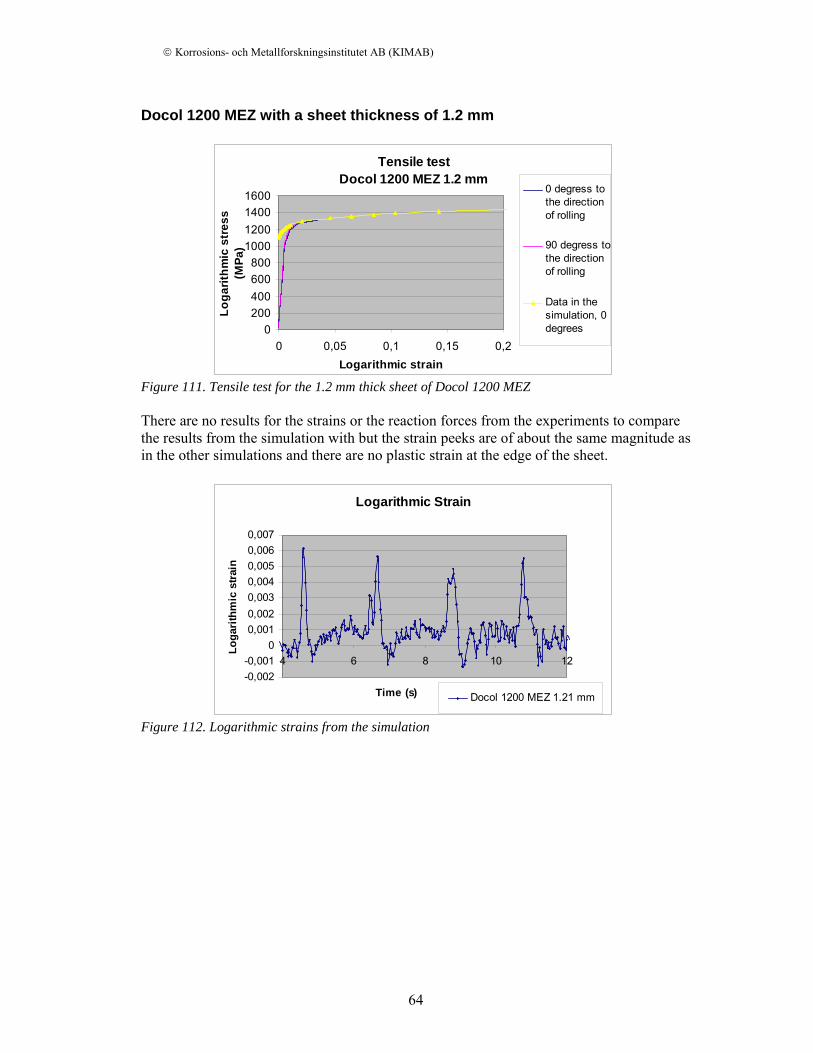
© Korrosions- och Metallforskningsinstitutet AB (KIMAB)
64
Docol 1200 MEZ with a sheet thickness of 1.2 mm
Tensile testDocol 1200 MEZ 1.2 mm
0200400600800
1000120014001600
0 0,05 0,1 0,15 0,2Logarithmic strain
Loga
rithm
ic s
tres
s (M
Pa)
0 degress tothe directionof rolling
90 degress tothe directionof rolling
Data in thesimulation, 0degrees
Figure 111. Tensile test for the 1.2 mm thick sheet of Docol 1200 MEZ There are no results for the strains or the reaction forces from the experiments to compare the results from the simulation with but the strain peeks are of about the same magnitude as in the other simulations and there are no plastic strain at the edge of the sheet.
Logarithmic Strain
-0,002-0,001
00,0010,0020,0030,0040,0050,0060,007
4 6 8 10 12
Time (s)
Loga
rithm
ic s
train
Docol 1200 MEZ 1.21 mm
Figure 112. Logarithmic strains from the simulation
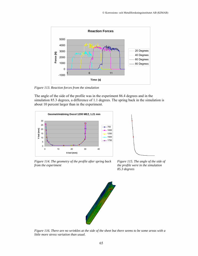
© Korrosions- och Metallforskningsinstitutet AB (KIMAB)
65
Reaction Forces
-1000
0
1000
2000
3000
4000
5000
1 6 11
Time (s)
Forc
e (N
) 20 Degrees40 Degrees60 Degrees80 Degress
Figure 113. Reaction forces from the simulation The angle of the side of the profile was in the experiment 86.4 degrees and in the simulation 85.3 degrees, a difference of 1.1 degrees. The spring back in the simulation is about 10 percent larger than in the experiment.
Geometrimätning Docol 1200 MEZ, 1.21 mm
0
5
10
15
20
25
30
0 10 20 30 40
X-led (mm)
Y-le
d (m
m) 750
1000125015001750
Figure 114. The geometry of the profile after spring back from the experiment
Figure 115. The angle of the side of the profile were in the simulation 85.3 degrees
Figure 116. There are no wrinkles at the side of the sheet but there seems to be some areas with a little more stress variation than usual.
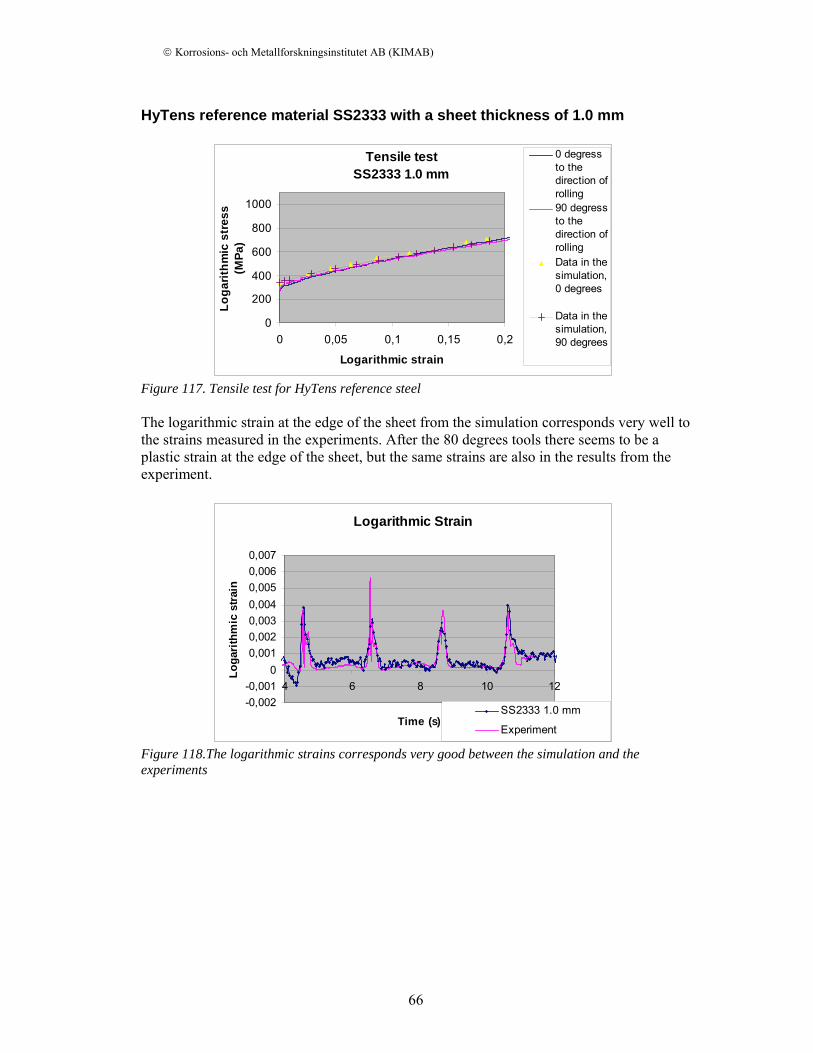
© Korrosions- och Metallforskningsinstitutet AB (KIMAB)
66
HyTens reference material SS2333 with a sheet thickness of 1.0 mm
Tensile testSS2333 1.0 mm
0
200
400
600
800
1000
0 0,05 0,1 0,15 0,2
Logarithmic strain
Loga
rithm
ic s
tres
s (M
Pa)
0 degressto thedirection ofrolling90 degressto thedirection ofrollingData in thesimulation,0 degrees
Data in thesimulation,90 degrees
Figure 117. Tensile test for HyTens reference steel The logarithmic strain at the edge of the sheet from the simulation corresponds very well to the strains measured in the experiments. After the 80 degrees tools there seems to be a plastic strain at the edge of the sheet, but the same strains are also in the results from the experiment.
Logarithmic Strain
-0,002-0,001
00,0010,0020,0030,0040,0050,0060,007
4 6 8 10 12
Time (s)
Loga
rithm
ic s
trai
n
SS2333 1.0 mm
Experiment
Figure 118.The logarithmic strains corresponds very good between the simulation and the experiments
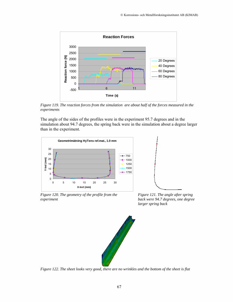
© Korrosions- och Metallforskningsinstitutet AB (KIMAB)
67
Reaction Forces
-500
0
500
1000
1500
2000
2500
3000
1 6 11
Time (s)
Reac
tion
forc
e (N
)20 Degrees40 Degrees60 Degrees80 Degrees
Figure 119. The reaction forces from the simulation are about half of the forces measured in the experiments The angle of the sides of the profiles were in the experiment 95.7 degrees and in the simulation about 94.7 degrees, the spring back were in the simulation about a degree larger than in the experiment.
Geometrimätning HyTens ref.mat., 1.0 mm
0
5
10
15
20
25
30
0 5 10 15 20 25 30
X-led (mm)
Y-le
d (m
m) 750
1000125015001750
Figure 120. The geometry of the profile from the experiment
Figure 121. The angle after spring back were 94.7 degrees, one degree larger spring back
Figure 122. The sheet looks very good, there are no wrinkles and the bottom of the sheet is flat
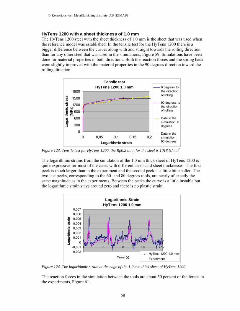
© Korrosions- och Metallforskningsinstitutet AB (KIMAB)
68
HyTens 1200 with a sheet thickness of 1.0 mm The HyTens 1200 steel with the sheet thickness of 1.0 mm is the sheet that was used when the reference model was established. In the tensile test for the HyTens 1200 there is a bigger difference between the curves along with and straight towards the rolling direction than for any other steel that was used in the simulations, Figure 59. Simulations have been done for material properties in both directions. Both the reaction forces and the spring back were slightly improved with the material properties in the 90 degrees direction toward the rolling direction.
Tensile testHyTens 1200 1.0 mm
0
300
600
900
1200
1500
1800
0 0,05 0,1 0,15 0,2Logarithmic strain
Loga
rithm
ic s
tres
s (M
Pa)
0 degress tothe directionof rolling
90 degress tothe directionof rolling
Data in thesimulation, 0degrees
Data in thesimulation,90 degrees
Figure 123. Tensile test for HyTens 1200, the Rp0.2 limit for the steel is 1018 N/mm2 The logarithmic strains from the simulation of the 1.0 mm thick sheet of HyTens 1200 is quite expressive for most of the cases with different steels and sheet thicknesses. The first peek is much larger than in the experiment and the second peek is a little bit smaller. The two last peeks, corresponding to the 60- and 80 degrees tools, are nearly of exactly the same magnitude as in the experiments. Between the peeks the curve is a little instable but the logarithmic strain stays around zero and there is no plastic strain.
Logarithmic StrainHyTens 1200 1.0 mm
-0,002-0,001
00,0010,0020,0030,0040,0050,0060,007
4 6 8 10 12
Time (s)
Loga
rithm
ic s
train
HyTens 1200 1.0 mmExperiment
Figure 124. The logarithmic strain at the edge of the 1.0 mm thick sheet of HyTens 1200 The reaction forces in the simulation between the tools are about 50 percent of the forces in the experiments, Figure 61.
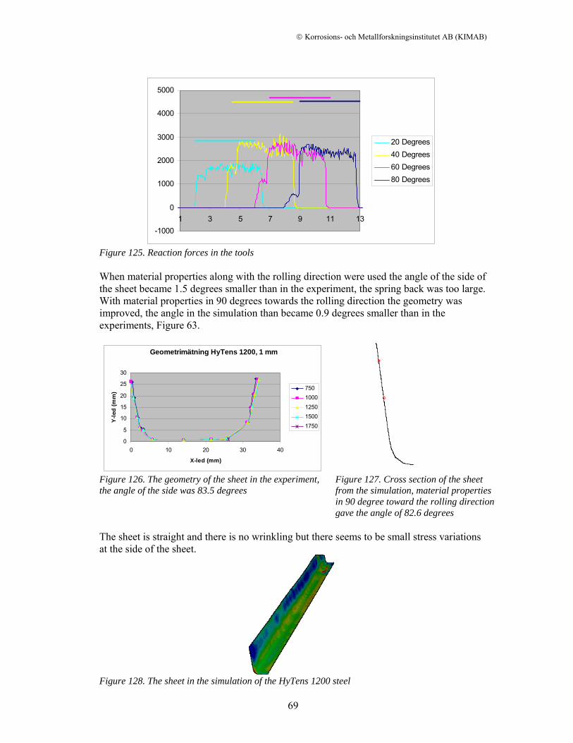
© Korrosions- och Metallforskningsinstitutet AB (KIMAB)
69
-1000
0
1000
2000
3000
4000
5000
1 3 5 7 9 11 13
20 Degrees40 Degrees60 Degrees80 Degrees
Figure 125. Reaction forces in the tools When material properties along with the rolling direction were used the angle of the side of the sheet became 1.5 degrees smaller than in the experiment, the spring back was too large. With material properties in 90 degrees towards the rolling direction the geometry was improved, the angle in the simulation than became 0.9 degrees smaller than in the experiments, Figure 63.
Geometrimätning HyTens 1200, 1 mm
0
5
10
15
20
25
30
0 10 20 30 40
X-led (mm)
Y-le
d (m
m) 750
1000125015001750
Figure 126. The geometry of the sheet in the experiment, the angle of the side was 83.5 degrees
Figure 127. Cross section of the sheet from the simulation, material properties in 90 degree toward the rolling direction gave the angle of 82.6 degrees
The sheet is straight and there is no wrinkling but there seems to be small stress variations at the side of the sheet.
Figure 128. The sheet in the simulation of the HyTens 1200 steel
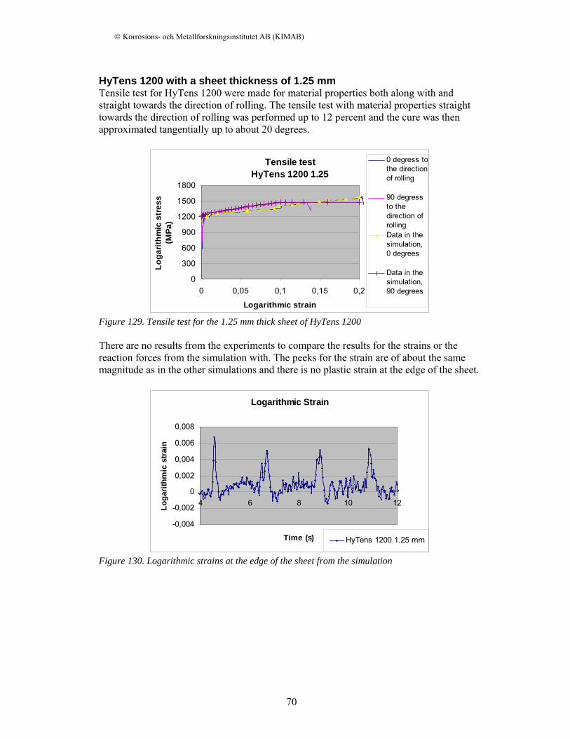
© Korrosions- och Metallforskningsinstitutet AB (KIMAB)
70
HyTens 1200 with a sheet thickness of 1.25 mm Tensile test for HyTens 1200 were made for material properties both along with and straight towards the direction of rolling. The tensile test with material properties straight towards the direction of rolling was performed up to 12 percent and the cure was then approximated tangentially up to about 20 degrees.
Tensile testHyTens 1200 1.25
0
300
600
900
1200
1500
1800
0 0,05 0,1 0,15 0,2
Logarithmic strain
Loga
rithm
ic s
tres
s (M
Pa)
0 degress tothe directionof rolling
90 degressto thedirection ofrollingData in thesimulation,0 degrees
Data in thesimulation,90 degrees
Figure 129. Tensile test for the 1.25 mm thick sheet of HyTens 1200 There are no results from the experiments to compare the results for the strains or the reaction forces from the simulation with. The peeks for the strain are of about the same magnitude as in the other simulations and there is no plastic strain at the edge of the sheet.
Logarithmic Strain
-0,004
-0,002
0
0,002
0,004
0,006
0,008
4 6 8 10 12
Time (s)
Loga
rithm
ic s
trai
n
HyTens 1200 1.25 mm
Figure 130. Logarithmic strains at the edge of the sheet from the simulation
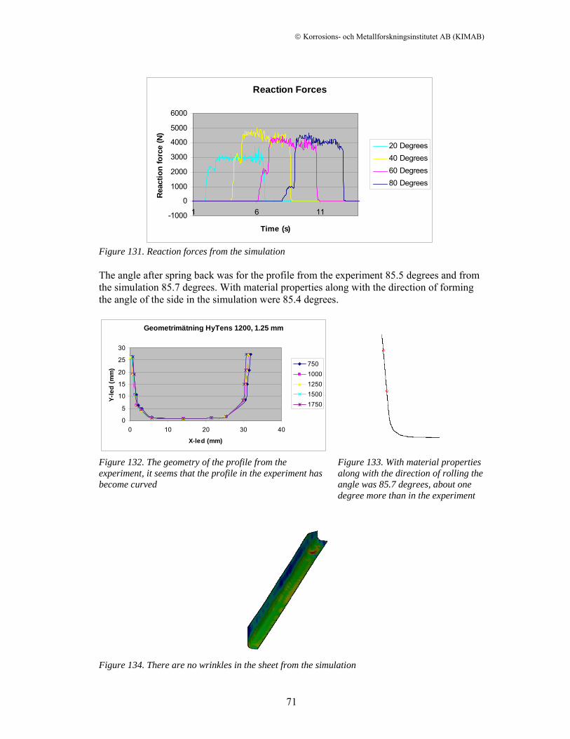
© Korrosions- och Metallforskningsinstitutet AB (KIMAB)
71
Reaction Forces
-1000
0
1000
2000
3000
4000
5000
6000
1 6 11
Time (s)
Reac
tion
forc
e (N
)
20 Degrees40 Degrees60 Degrees80 Degrees
Figure 131. Reaction forces from the simulation The angle after spring back was for the profile from the experiment 85.5 degrees and from the simulation 85.7 degrees. With material properties along with the direction of forming the angle of the side in the simulation were 85.4 degrees.
Geometrimätning HyTens 1200, 1.25 mm
0
5
10
15
20
25
30
0 10 20 30 40
X-led (mm)
Y-le
d (m
m) 750
1000125015001750
Figure 132. The geometry of the profile from the experiment, it seems that the profile in the experiment has become curved
Figure 133. With material properties along with the direction of rolling the angle was 85.7 degrees, about one degree more than in the experiment
Figure 134. There are no wrinkles in the sheet from the simulation
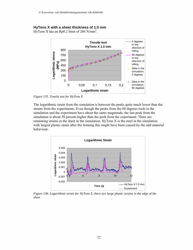
© Korrosions- och Metallforskningsinstitutet AB (KIMAB)
72
HyTens X with a sheet thickness of 1.0 mm HyTens X has an Rp0.2 limit of 286 N/mm2.
Tensile testHyTens X 1.0 mm
0150300450600750900
0 0,05 0,1 0,15 0,2
Logarithmic strain
Loga
rithm
ic s
tress
(M
Pa)
0 degressto thedirection ofrolling90 degressto thedirection ofrollingData in thesimulation,0 degrees
Data in thesimulation,90 degrees
Figure 135. Tensile test for HyTens X The logarithmic strain from the simulation is between the peeks quite much lower than the strains from the experiments. Even though the peeks from the 60 degrees tools in the simulation and the experiment have about the same magnitude, the last peek from the simulation is about 50 percent higher than the peek from the experiment. There are remaining strains in the sheet in the simulation. HyTens X is the steel in the simulation with largest plastic strain after the forming this might have been caused by the odd material behaviour.
Logarithmic Strain
-0,002
-0,001
0
0,001
0,002
0,003
0,004
0,005
4 6 8 10 12
Time (s)
Loga
rith
mic
stra
in
HyTens X 1.0 mmExperiment
Figure 136. Logarithmic strain for HyTens X, there are large plastic strains in the edge of the sheet
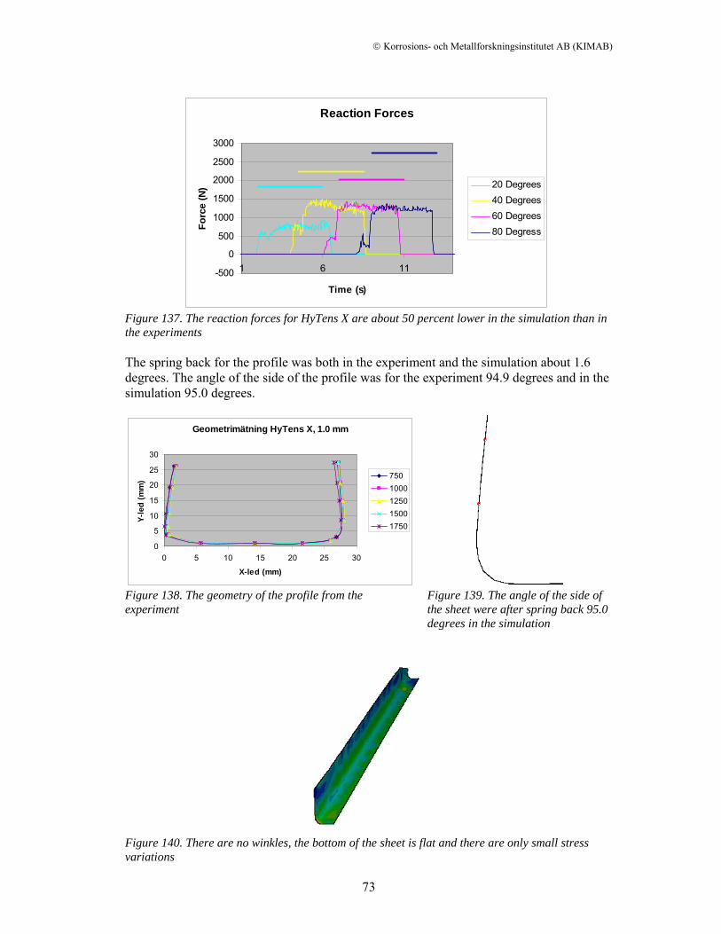
© Korrosions- och Metallforskningsinstitutet AB (KIMAB)
73
Reaction Forces
-500
0
500
1000
1500
2000
2500
3000
1 6 11
Time (s)
Forc
e (N
) 20 Degrees40 Degrees60 Degrees80 Degress
Figure 137. The reaction forces for HyTens X are about 50 percent lower in the simulation than in the experiments The spring back for the profile was both in the experiment and the simulation about 1.6 degrees. The angle of the side of the profile was for the experiment 94.9 degrees and in the simulation 95.0 degrees.
Geometrimätning HyTens X, 1.0 mm
0
5
10
15
20
25
30
0 5 10 15 20 25 30
X-led (mm)
Y-le
d (m
m) 750
1000125015001750
Figure 138. The geometry of the profile from the experiment
Figure 139. The angle of the side of the sheet were after spring back 95.0 degrees in the simulation
Figure 140. There are no winkles, the bottom of the sheet is flat and there are only small stress variations