Finite element method algorithm for geotechnical

This is an electronic reprint of the original article.This reprint may differ from the original in pagination and typographic detail.

Powered by TCPDF (www.tcpdf.org)

This material is protected by copyright and other intellectual property rights, and duplication or sale of all or part of any of the repository collections is not permitted, except that material may be duplicated by you for your research use or educational purposes in electronic or print form. You must obtain permission for any other use. Electronic or print copies may not be offered, whether for sale or otherwise to anyone who is not an authorised user.

Abed, Ayman A.; Sołowski, Wojciech T.Finite element method algorithm for geotechnical applications based on Runge-Kutta schemewith automatic error control

Published in:Computers and Geotechnics

DOI:10.1016/j.compgeo.2020.103841

Published: 01/12/2020

Document VersionPublisher's PDF, also known as Version of record

Published under the following license:CC BY

Please cite the original version:Abed, A. A., & Soowski, W. T. (2020). Finite element method algorithm for geotechnical applications based onRunge-Kutta scheme with automatic error control. Computers and Geotechnics, 128, [103841].https://doi.org/10.1016/j.compgeo.2020.103841

https://doi.org/10.1016/j.compgeo.2020.103841


Contents lists available at ScienceDirect

Computers and Geotechnics

journal homepage: www.elsevier.com/locate/compgeo

Research Paper

Finite element method algorithm for geotechnical applications based onRunge-Kutta scheme with automatic error controlAyman A. Abeda,b,⁎, Wojciech T. Sołowskiba Chalmers University of Technology, Department of Architecture and Civil Engineering, SE-412 96 Göteborg, SwedenbAalto University, Department of Civil Engineering, P.O. Box 12100, FI-00076 Aalto, Finland

A R T I C L E I N F O

Keywords:FEMExplicit methodsRunge-Kutta schemeAutomatic error control

A B S T R A C T

This paper introduces a novel explicit algorithm to solve the finite element equation linking the nodal dis-placements of the elements with the external forces applied via means of non-linear global stiffness matrix. Theproposed method solves the equation using Runge-Kutta scheme with automatic error control. The methodallows any Runge-Kutta scheme, with the paper demonstrating the algorithm efficiency for Runge-Kutta schemesof second to fifth order of accuracy. The paper discusses the theoretical background, the implementation stepsand validates the proposed algorithm. The numerical tests show that the proposed method is robust and stable.In comparison to the iterative implicit methods (e.g. Newton-Raphson method), the new algorithm overcomesthe problem of occasional divergence. Furthermore, considering the computation time, the fifth-order accuratescheme proves to be competitive with the iterative method. It seems that the proposed algorithm could be apowerful alternative to the standard solution procedures for the cases with strong nonlinearity, where the typicalalgorithms may diverge.

1. Introduction

The Finite Element Method approximates the solution of the con-tinuous mechanical balance equation by calculating the unknown dis-placement u at a set of discrete points only, typically at the elementnodes, as a response to the external load fext . This requires solving alarge set of equations, with coefficients given in the global stiffnessmatrix K where:

=Ku f 0ext (1)

In most engineering applications, the stiffness matrix K is changingin a non-linear fashion with the increment of external load fext . Thestiffness matrix nonlinearity can be a consequence of both the materialbehaviour and the geometric nonlinearity. In the common geotechnicalapplications, the material behaviour nonlinearity is dominant.Therefore, this paper disregards geometrical nonlinearity.

To solve Eq. (1), the Finite Element Method needs an efficient,stable and robust numerical algorithm. Typically the method of choicebelongs to the family of iterative Newton-Raphson scheme, for ex-ample: modified, initial stress or accelerated (Bathe, 2006), whichusually offers a satisfactory rate of convergence. Yet, the Newton-Raphson scheme requires the initial iteration result close enough (i.e.within the convergence radius) to the correct solution to converge and

an even closer result in order to get the quadratic rate of convergence.On the other hand, if the load increment is large compared to the non-linearity of the problem, the initial iteration result may fall outside ofthe convergence radius and the Newton-Raphson scheme may fail toreach the solution. If this happens, the codes after significant number ofiterations usually cut the load increment to half and repeat the process,hoping that the convergence will be reached. If that does not work,ultimately, the solution may be abandoned with an error (Section 8gives an example of such situation).

The method also requires the evaluation of the inverse of theJacobian (first order derivatives) matrix at each iteration which im-poses additional numerical expense and difficulties in a large system ofequations. To avoid the problems related to the repetitive calculation ofthe Jacobian, the quasi-Newton methods evolved (e.g. Broyden-Fletcher-Goldfarb-Shanno (BFGS)) (Matthies and Strang, 1979; Avriel,2003). The main idea behind this class of methods is that the Jacobianmatrix in Newton-Raphson scheme needs to be estimated only in thefirst iteration and then, in the subsequent iterations, it will be ap-proximated based on the Jacobian from the previous iteration. In theoriginal contribution, Brayden (Broyden, 1965) even proposed a for-mula to update the Jacobian inverse directly based on the inverse of thepreceding iteration which would further save the computational effort.Although the quasi-Newton methods offer occasionally successful

https://doi.org/10.1016/j.compgeo.2020.103841Received 4 March 2020; Received in revised form 10 September 2020; Accepted 12 September 2020

⁎ Corresponding author at: Chalmers University of Technology, Department of Architecture and Civil Engineering, SE-412 96 Göteborg, Sweden.E-mail address: [email protected] (A.A. Abed).

Computers and Geotechnics 128 (2020) 103841

0266-352X/ © 2020 The Author(s). Published by Elsevier Ltd. This is an open access article under the CC BY license (http://creativecommons.org/licenses/BY/4.0/).

T

http://www.sciencedirect.com/science/journal/0266352X

https://www.elsevier.com/locate/compgeo



mailto:[email protected]


http://crossmark.crossref.org/dialog/?doi=10.1016/j.compgeo.2020.103841&domain=pdf

alternative when the classical Newton-Raphson scheme fails, they stillrequire the initial guess to be close to the correct solution to ensureconvergence.

Gens and Potts (1988) carried out an early study on the differentmethods used to solve nonlinear equations in geotechnical applicationswith a constitutive model based on the critical state concept. The studyincluded, in addition to the iterative procedures, the explicit first-orderforward Euler scheme (tangent stiffness method). They concluded thatthere is no generic statement on the recommended method to be usedand it is necessary to equip the numerical code with different solutionmethods so that the most suitable one can be used depending on thesolved problem. In a later study, however, Potts and Ganendra (1992)concluded that the modified Newton-Raphson method is the most ro-bust and economical method, which is now the standard in most of theFinite Element codes. To improve the convergence of the scheme,several numerical techniques can be used, including the arc length

control and the line search method (Bathe, 2006; Crisfield, 1983).Abbo and Sloan (1996) provided an improved second-order explicit

scheme (Euler-modified Euler) with error control of the drift from theload path. Although, the scheme showed to be robust and stable even inapplications that involve critical state soil models (Sheng and Sloan,2001), the iterative methods were significantly faster, hence the schemewas not widely adopted. Recently, the numerical software started in-cluding the automatic (algorithmic) differentiation (AD) (Griewank andWalther, 2008), which means that the accurate derivation of the stiff-ness matrix is available without extra numerical burden. This opensnew possibilities for novel numerical algorithms, more stable and ro-bust than existing ones.

2. Importance and significance of the proposed method

This paper presents a novel alternative method which treats Eq. (1)

Nomenclature

Roman

DTol tolerated displacement errorErr error vectorError scalar error measurefext external forces vector, M LT−2

fint internal nodal forces vector, M LT−2

F yield functionITol tolerated error for iterative procedureK global stiffness matrixKo coefficient of at rest earth pressureKo

NC coefficient of at rest earth pressure for normally con-solidated soil

m number of nodes in the meshM slope of critical state linen Runge-Kutta scheme ordernsub number of sub-incrementsp' isotropic effective pressure, M L−1T−2

pc isotropic preconsolidation pressure, M L−1T−2

POP pre-overburden pressure, M L−1T−2

q deviatoric stress, M L−1T−2

r force residual, M LT−2

s number of stages in Runge-Kutta schemet time at the end of a loading incrementto time at the start of a loading incrementtref reference timeT dimensionless timev0 initial specific volume

Greek

factor to control the size of load increment growthkj Runge-Kutta scheme coefficient

factor to control substep sizesafety factor to control the size of load incrementunloading-reloading index

µ Poisson’s ratio' effective Cauchy stress tensor, M L−1T−2

plastic compression indexk Runge-Kutta scheme coefficientf force increment, M LT−2

t time incrementT dimensionless time incrementTmin minimum dimensionless time incrementu displacement increment vector, L

Fig. 1. Implicit methods: iterations per the ith load increment to estimate the corresponding displacement increment.

A.A. Abed and W.T. Sołowski Computers and Geotechnics 128 (2020) 103841

2

as a differential equation and applies Runge-Kutta explicit schemes withautomatic sub-incrementation (sub-stepping) and error control to solveit. The paper discusses first the theoretical background and the nu-merical implementation steps. Subsequently, the method is tested on atypical geotechnical problem of a shallow foundation resting on anelastoplastic soil. In the tests, the new method has been more stablethan most common existing solutions. The proposed algorithm based onthe 5th order Runge-Kutta scheme is also competitive with the iterativeschemes regarding the time of calculations.

The new method of solution builds on a well-tested, robust schemewith mathematically proven convergence properties. Consequently, itsadoption may be beneficial not only in the Finite Element software forgeotechnical engineering, but in all Finite Element codes used foranalysis of highly non-linear problems, for instance coupled thermo-hydro-mechanical-chemical analyses.

3. Solution algorithm

In the case of nonlinear material behaviour, the stiffness matrix inEquation (1) depends on stresses and strains. Those are related to dis-placements, hence the stiffness matrix is ultimately displacement de-pendent =K u f u( ) /int , where fint is the vector of internal nodalforces. This allows us to rewrite Equation (1) as a differential equation:

=t tu K u fd /d [ ( )] d /di i1 (2)

where ud i is the infinitesimal increment of displacements and fd i is theinfinitesimal increment of externally applied forces over an algorithmictime infinitesimal increment td . The dependency of stiffness matrix ondisplacements stems from the complex constitutive behaviour of soil(material) which, in most cases, involves nonlinear elasticity andplasticity. Typically, Eq. (2) is solved incrementally allowing for line-arization by applying the total external force in increments fi per eachtime increment t . To enhance the mathematical clarity of Eq. (2), oneintroduces the dimensionless time = t t tT ( )/d0 where t and t0 are thealgorithmic time at the end and at the start of the load increment re-sulting in 0 T 1. Then, following the chain rule, the incrementaldisplacements per time increment will be = ×t tu ud /d d /dT 1/di i .Substitution in Equation (2) yields:

=u K u fd /dT [ ( )] di i i1 (3)

Eq. (3) is a first-order ordinary nonlinear differential equationwhich can be solved using iterative methods (implicit) such as the

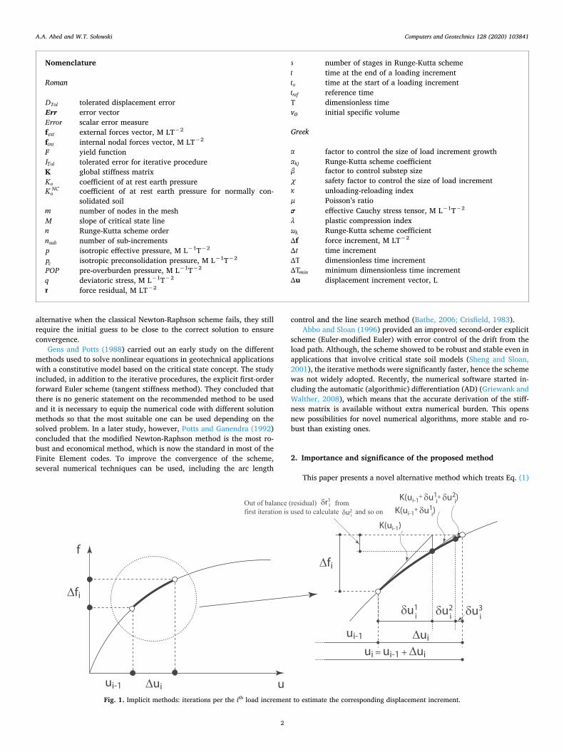
Newton-Raphson method. Other possibility is to use the explicitmethods that solve the equation directly without iterations but assumeload increments fi that satisfy certain accuracy condition. Fig. 1 andFig. 2 show, for a one-dimensional case, how both methods approachthe solution ui for the ith load increment fi. Based on Eq. (3), for eachload increment fi, one calculates the corresponding displacement in-crement ui and adds this value to the previously calculated total dis-placements ui 1 to determine the new ui. The solution starts withknown initial displacement u0, thus Eq. (3) is an initial value problem.

Despite the rapid convergence rate of the implicit methods, theirconvergence is conditional as the initial prediction needs to be suffi-ciently close to the correct solution. Therefore, the Newton-Raphsonmethod divergence happens especially often in the case of materialbehaviour with strong nonlinearity. Another major disadvantage of theimplicit methods is that they do not have any load path error controlmeaning that it could converge if big loading increments are adopted,but to a wrong answer (Abbo and Sloan, 1996). On the other hand, theexplicit methods are stable; however, the only explicit method com-monly used in the past, the Forward Euler method, tends to drift awayfrom the correct solution with the advancement of the solution. Tocontrol the drift, small load increments should be adopted which slowdown the solution tremendously and make the Forward Euler methodunattractive.

Although the explicit Runge-Kutta methods received wide recogni-tion for integrating constitutive laws on the Gauss point level (Sloan,1987; Sloan et al., 2001; Sołowski and Gallipoli, 2010), they got littleattention on their applicability for solving the global finite elementequations. Apart from the contribution by Abbo and Sloan (1996) whoproposed an explicit scheme with error control that can be consideredas a second-order scheme when compared to the first-order ForwardEuler scheme, the authors are not aware of any other major contribu-tion.

When solving Eq. (3) with Runge-Kutta method, the estimation ofui is taken as a weighted sum of explicit evaluations of ui

k( ) at pre-defined positions k along the given algorithmic time interval T. Thenumber of these evaluations is directly related to the required accuracyof the solution, yielding a scheme with different orders (e.g. first,second … fifth and higher). Employing a high order Runge-Kuttascheme leads to a fast convergence and an accurate solution with wellcontrolled errors. It should be noted that the Runge-Kutta method is astandard numerical method that can be reviewed elsewhere, see Leeand Schiesser (2003) for example.

Fig. 2. Explicit methods: (a) first-order forward Euler and (b) second-order estimate of displacement increment per the ith load increment.


3

4. Runge-Kutta explicit scheme for load-deflection estimation

The first-order Runge-Kutta method is equivalent to the forwardexplicit Euler method where the displacement increment is the directoutcome of Eq. (3) with =dT 1, see Fig. 2 and Eq. (4). Obviously, theaccuracy of the first-order scheme is heavily dependent on the loadincrement size. To achieve a sufficiently accurate solution, very smallincrements should be adopted leading to a numerically expensive so-lution. For Runge-Kutta second-order scheme, the estimation of thedisplacement increment ui needs two stages =k( 1, 2) of secondarydisplacement increment evaluations ui

k( ) (see Fig. 2 for a graphicalclarification):

Stage =k 1:

=u K u f[ ( )]i i i(1)

1(1) 1 (4)

Stage =k 2:

= +u K u u f[ ( )]i i i i(2)

1(1) 1 (5)

where K is the displacement-dependent tangent stiffness matrix with=K u f u( ) /i int i1

(1) (1)1 and + = +K u u f u u( ) / ( )i i int i i1

(1) (2)1

(1) . Notethat f int

(1) and f int(2) represent the internal forces at the corresponding

displacements ui 1 and +u ui i1(1) , respectively. Consequently, the

second order estimation of the displacement increment ui is:

= + = +u u u u u12

12

12

( )i i i i i(1) (2) (1) (2)

(6)

As can be noticed, the weighing factors are identical here for thetwo estimations and equal ½. One important aspect to mention is thatseveral Runge-Kutta methods have embedded a lower order solution,which can be used to estimate the error. This error is given as the dif-ference between the current scheme displacement estimation and theestimation with the one order lower scheme. For example, for thesecond-order scheme presented above, the error Err is given as:

= = + + +

=

Err u u u u u u u

u u

12

( ) [ ]

12

( )

i i i

second order estimate

i ifirst order estimate

i i

(2nd) (2nd) (1st)1

(1) (2)1

(1)

(2) (1)(7)

Runge-Kutta schemes with higher order of accuracy follow a similaralgorithm. By knowing the correct weights and positions to estimateeach secondary stage evaluation, the displacement increment is de-termined as a weighted sum of the performed evaluations. For an ar-bitrary high order method, Eq. (4) and Eq. (5) read:

=u K u f[ ( )]ik

ik

i( ) ( ) 1 (8)

where

= +=

u u uik

ij

k

kj ij( )

11

1( )

(9)

Here uik( ) represents the updated displacements according to the

adopted Runge-Kutta scheme. The stiffness matrix=K u f u u( ) ( )/i

kintk

ik

ik( ) ( ) ( ) ( ) where f u( )int

kik( ) ( ) indicates the corresponding

displacement dependent internal forces to the displacement’s evalua-tion ui

k( ) at the calculation stage k. In this contribution, the evaluation

of the stiffness matrix K u( )ik( ) is carried out using the automatic dif-

ferentiation (AD) during the finite elements assembly process as will bediscussed later. The estimated displacements are then calculated as:

= +=

u u uin

ik

s

k ik( )

11

( )

(10)

where s is the total number of evaluation stages that is dependent onthe scheme order n (Lee and Schiesser, 2003).

By subtracting the lower order solution from the one order highersolution, the error can be estimated as:

==

Err un

k

s

k ik( )

1

( )

(11)

Tables 1–6 give the coefficients kj, k and k for Eqs. (9), (10) and(11) for Runge-Kutta schemes of 2nd, 3rd, 4th and 5th order. Note thatany Runge-Kutta scheme, e.g. those given in (Lee and Schiesser, 2003),can be used – tables give only the coefficients for schemes tested in thispaper.

5. Runge-Kutta explicit scheme with error control

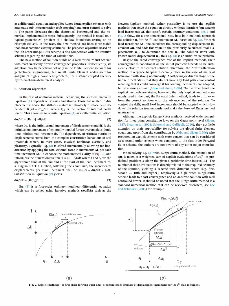
The error in the Runge-Kutta scheme is dependent on the size of theload increment fi. For the same increment size, the higher-orderschemes yield predictions that are more accurate. Additionally, themethod assesses the error which can be used to automatically choosethe next load increment size, so that the error is bound within a de-sirable range, similarly as in the case of stress integration (Abbo andSloan, 1996; Sloan, 1987; Sołowski and Gallipoli, 2010). The proposedsteps of the method to solve the global finite element equations areillustrated in Diagram 1 and listed in Table 7.

The scheme starts by assuming that the first load sub-increment= ×f fTj j i, where j = 1 is the number of the current sub-incre-

ment, equals the full load increment fi by using an initial sub-incre-ment size of Tj = 1. After calculating the corresponding displacementusing f j by employing Eq. (9) and Eq. (10), the occurred relative errorError is estimated by applying Eq. (11). If this error is less or equal tothe imposed tolerance DTol by the user, the current sub-increment isaccepted and the program moves to the next load increment (seeDiagram 1 and Table 7). On the other hand, if the error is greater thanDTol, the current sub-increment is rejected and instead of Tj = 1, a newsmaller value is estimated using Eq. (12). At this point the calculationsare repeated with the new sub-increment size. The algorithm willcontinue reducing the increment size until the error criterion is satisfiedand the step is accepted.

For both accepted and rejected sub-increments, a new sub-incre-ment size is estimated again using Eq. (12). The procedure continuesuntil the full increment is applied yielding = =f fi j

n1 j

sub where= ×f fTj j i, == T 1j

n1 j

sub and nsub is the resulted total number ofaccepted sub-increments.

The size of the new sub-increment Tnew is estimated based on theold given sub-increment size Told, the scheme order of accuracy n andthe estimated error Error in the current sub-increment. Thus, the new

Table 1Stages for the 2nd order scheme.

Item Estimate

Stage 1 displacement estimate: =u K u f[ ( )]i i i(1)

1 1

Stage 2 displacement estimate: = +u K u u f[ ( )]i i i i(2)

1(1) 1

Second order displacement estimate: = + +u u u u( )i i i ind(2 )

112

(1) (2)

Error =Err u u( )i ind(2 ) 1

2(2) (1)

Table 2Stages for the 3rd order scheme.

Item Estimate


1 1

Stage 2 displacement estimate:= +( )u K u u fi i i i

(2)1

23

(1) 1

Stage 3 displacement estimate:= +( )u K u u fi i i i

(3)1

23

(2) 1

Third order displacement estimate: = + + +u u u u ui i i i ird(3 )

128

(1) 38

(2) 38

(3)

Error =Err u u( )i ird(3 ) 3

8(3) (2)


4

sub-increment size is = ×T Tnew old where:

= DError

Toln(12)

Here, is the relative change in the next sub-increment size, DTol is

the required accuracy imposed by the user and is a safety factor, asthis sub-increment size estimation is approximate. Such a choice of thenew sub-increment size should keep the error in the next step below thetolerated value (Gustafsson, 1992). To reduce the chance of spuriousincrease/decrease of the steps due to random correlation between the

Table 3Stages for the 4th order scheme.

Item Estimate


1 1


1 21(1) 1

Stage 3 displacement estimate: = + +u K u u u f[ ( )]i i i i i(3)

1 31(1)

32(2) 1

Stage 4 displacement estimate: = + + +u K u u u u f[ ( )]i i i i i i(4)

1 41(1)

42(2)

43(3) 1

Fourth order displacement estimate: = + + + +u u u u u ui i i i i ith(4 )

1 1(1)

2(2)

3(3)

4(4)

Error = + + +Err u u u ui i i ith(4 ) 1

(1)2

(2)3

(3)4

(4)

*Table 4 lists the corresponding coefficients.

Table 4Coefficients for the 4th order scheme.

Item Coefficient value

Stage 2 21−0.4

Stage 3 31 320.6684895833 −0.2434895833

Stage 4 41 42 43−2.323685857 1.125483559 2.198202298

Displacement 1 2 3 40.03431372549 0.02705627706 0.7440130202 0.1946169772

Error 1 2 3 40.03431372549 −0.01262626262 −0.0289338397 0.00724637679

Table 5Stages for the 5th order scheme.

Item Estimate


1 1


1 21(1) 1

Stage 3 displacement estimate: = + +u K u u u f[ ( )]i i i i i(3)

1 31(1)

32(2) 1

Stage 4 displacement estimate: = + + +u K u u u u f[ ( )]i i i i i i(4)

1 41(1)

42(2)

43(3) 1

Stage 5 displacement estimate: = + + + +u K u u u u u f[ ( )]i i i i i i i(5)

1 51(1)

52(2)

53(3)

54(4) 1

Stage 6 displacement estimate: = + + + + +u K u u u u u u f[ ( )]i i i i i i i i(6)

1 61(1)

62(2)

63(3)

64(4)

65(5) 1

Fifth order displacement estimate: = + + + + + +u u u u u u u ui i i i i i i ith(5 )

1 1(1)

2(2)

3(3)

4(4)

5(5)

6(6)

Error = + + + + +Err u u u u u ui i i i i ith(5 ) 1

(1)2

(2)3

(3)4

(4)5

(5)6

(6)

* Table 6 lists the corresponding coefficients in the case of 5th order scheme.

Table 6Coefficients for the 5th order scheme.

Item Coefficient value

Stage 2 211/5

Stage 3 31 323/40 9/40

Stage 4 41 42 433/10 −9/10 6/5

Stage 5 51 52 53 54−11/54 5/2 −70/27 35/27

Stage 6 61 62 63 64 651631/55296 175/512 575/13824 44275/110592 253/4096

Displacement 1 2 3 4 5 637/378 0 250/621 125/594 0 512/1771

Error 1 2 3 4 5 6−277/64512 0 6925/370944 −6925/202752 −277/14336 277/7084


5

two solutions used for estimation of the error and to avoid unnecessaryfailed sub-increment sizes, the resulted from Eq. (12) is limited byvalue of and 0.1. Previous experience (Abbo and Sloan, 1996; Sloanet al., 2001) showed that the recommended values are in the range0.7 0.9 and 1.1 2.0. The authors used the values = 0.9 and

= 1.2, leading to 0.1 1.2 in the calculations. This means that theincrease of the next load sub-increment is capped at 120% of the cur-rent load sub-increment. As can be interpreted from Eq. (12), the newsub-increment size will be reduced in case of rejected step( >Error DTol).

6. Note on the evaluation of the global stiffness matrix byautomatic differentiation

The evaluation of the global stiffness matrix is an important stepduring the solution for displacement increment as given by Eq. (8).Typically, that would need the assembly of the global stiffness matrixfrom the individual finite element stiffness matrices respecting the

relevant degrees of freedom (Smith et al., 2013). Thebes code (Abedand Sołowski, 2017, 2019), based on Numerrin numerical solver(Laitinen, 2013), follows a different method to evaluate the stiffnessmatrix by the direct differentiation of the internal nodal forces withrespect to the current nodal displacements. That is carried out using theautomatic (algorithmic) differentiation (AD) (Griewank and Walther,2008) where the stiffness matrix is evaluated during the assembly of theinternal nodal forces. The main idea behind AD is that any function isexecuted as a sequence of basic operations (e.g. additions, subtractions,multiplications, etc.). By applying the chain rule repeatedly to theseoperations, the derivative of such a function can be computed with notruncation errors (i.e. to the machine precision). In order to achievethat, a parallel program translates the code of the respective function(that is not necessarily present in closed form but most of the time as acomputer program) into a new code that contains derivatives. The ap-plication of this method is not well recognized in the field of compu-tational geomechanics but has received full consideration in the generalfield of the finite element method (Tijskens et al., 2002; Rothe and

Diagram 1. A flow chart illustrates the required steps by the proposed Runge-Kutta scheme.


6

Hartmann, 2015; Zwicke et al., 2016; Mitusch, 2018). The theoreticaldetails of algorithmic differentiation are out of the scope of this paper,however the interested reader is referred to (Griewank and Walther,2008; Bischof et al., 1992, 1996) for more details. In any case, the waythe global stiffness matrix is determined does not affect the essence ofthe proposed method for solving the finite element equations.

7. Comparison of a single Newton-Raphson iteration versus oneRunge-Kutta calculation stage

To assess the efficiency of the proposed scheme, we compare it tothe Newton-Raphson scheme, typically used in Finite Element Methodcalculations. During a standard full Newton-Raphson iteration k withinthe load increment (step) i, the following operations are performed:

1. Form the tangent stiffness matrix KT (Jacobian matrix) at the esti-mated displacement from previous iteration:

=K u ru

( )ik i

k

ikT

2. Compute the improvement in displacement value uik

=u K u r[ ( )]ik

ik

ik

T1

3. Compute the new displacements +uik 1 to be used in the next iteration

+k 1

=+u u uik

ik

ik1

where =r f fext int is the force residual (out of balance) vector. Theiterations continue until the imposed convergence criterion is satisfied.

On the other hand, the operations for one stage k of Runge-Kuttaschemes follow the steps:

1. Evaluate the stiffness matrix for a stage k using the estimated dis-placements for that stage:

Table 7Required steps to integrate the global finite element equations using the Runge-Kutta scheme.

1. Enter with the estimated total displacements from the previous loading incrementui 1, the applied load fi 1, the new load increment fi. Provide values for thetolerated error DTol, the minimum load increment size ΔTmin, the safety factor forload increment size χ and the threshold value to control the maximum growth ofthe next load increment α. Choose the required order of the Runge-Kutta scheme(n). Initialize T = 0 and T1 = 1.2. Loop as long as < =T 1 and perform a to d, otherwise, go to Step 3a. Based on the chosen order of Runge-Kutta scheme (n), evaluate thedisplacements for each stage k using formula (9) together with the correspondingcoefficients in Tables 1–6. Use = ×f fTj j i in the formula. The subscript jindicates the number of the current sub-increment. Note that the global stiffnessmatrix at each stage k is evaluated directly by the algorithmic differentiation ofthe generated internal nodal forces f int

k( ) with respect to the correspondingupdated displacements ui

k( ) .b. Estimate the displacements at the end of the load sub-increment u j

n( ) using Eq.(10) depending on the scheme order n( ).

c. Estimate the error vector Err n( ) based on Eq. (11) depending on the chosenscheme order, then estimate the relative error:

=Error Err u/njn( ) ( )

For the 2D case, the error norm Err n( ) is calculated as:= + + + +Err Err Err ErrErr (0) (1) (0) (1)n n n

mn

mn( )

1( )2

1( )2 ( )2 ( )2

where Err is the displacement error component being estimated, according to eachorder, based on Tables 1–6 and m is the total number of nodes in the mesh. Note thatErr (0) and Err (1) represent the error in estimating the displacement increment of thecalculated node in x and y direction, respectively.d. Check the condition Error DTol:i. If yes, estimate the new load increment size +Tj 1 based on the factor , update

= ++T T Tj 1 and repeat from Step 2, where:= = = ×+; min( , ); T TDTol

Errorn j j1

Apply the following constraints on the new sub-increment to avoid very small sizes oroverloading once approaching the completion of the current load increment i.

= =+ + + +T max( T , T ); T min( T , 1.0 T)j j min j j1 1 1 1ii. If >Error DTol then reject the current load sub-increment, estimate a new “smaller”load sub-increment = ×T Tj j and repeat from Step 2.

= DTolError

n

Apply the following constraints on the new reduced sub-increment to avoid verysmall sizes.= = ×max( , 0.1); T max( T , T )j j min3. Exit with the new displacements = + =u u ui

ni j

nsub( )1 1 j, update stresses and state

variables and continue to the new load increment +i 1.

Fig. 3. Modified Cam Clay model: a) isotropic loading-unloading in v-ln p′ plane; b) yield surface in p′-q plane.

Table 8Modified Cam Clay parameters of the modelled clay layer.

μ κ λ M v0 POP [kPa]

0.3 0.02 0.2 1.0 2.3 20.0


7

=K u f uu

( ) ( )ik int

kik

ik

( )( ) ( )

( )2. Calculate the displacement increment using the estimated stiffnessmatrix in Step 1 and the provided loading increment:

=u K u f[ ( )]ik

ik

i( ) ( ) 1

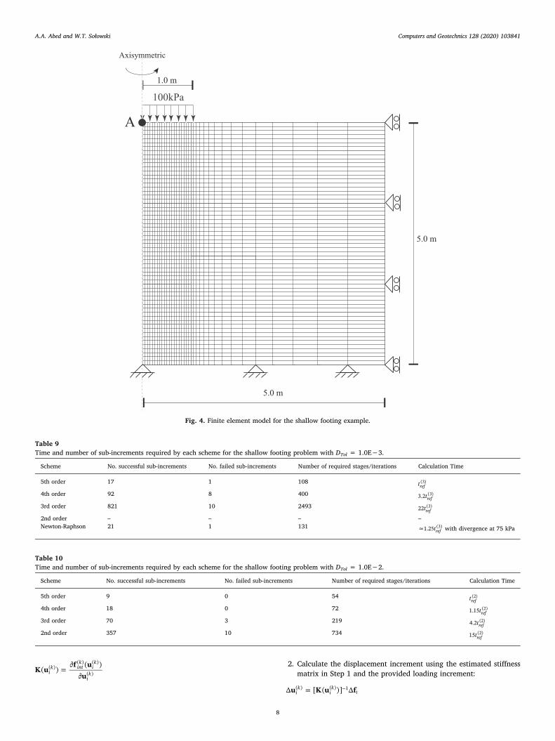
Fig. 4. Finite element model for the shallow footing example.

Table 9Time and number of sub-increments required by each scheme for the shallow footing problem with DTol = 1.0E−3.

Scheme No. successful sub-increments No. failed sub-increments Number of required stages/iterations Calculation Time

5th order 17 1 108 tref(3)

4th order 92 8 400 t3.2 ref(3)

3rd order 821 10 2493 t22 ref(3)

2nd order – – – –Newton-Raphson 21 1 131 ≈ t1.25 ref

(3) with divergence at 75 kPa




4th order 18 0 72 t1.15 ref(2)

3rd order 70 3 219 t4.2 ref(2)

2nd order 357 10 734 t15 ref(2)


8

3. Calculate the displacements to be used in the next stage +k 1:

= ++

=u u ui

ki

j

k

kj ij( 1)

11

( )

By comparison, one notices that the number of computational op-erations in a single iteration of Newton-Raphson method is roughlycomparable to that performed during one stage of a Runge-Kuttascheme (though the Runge-Kutta method does require more summationoperations in Step 3 to estimate the displacements at the required




4th order 16 0 64 t1.03 ref(1)

3rd order 17 0 51 t0.9 ref(1)

2nd order 43 3 92 t1.9 ref(1)

Fig. 5. Numerical results with 3rd order scheme and different tolerated errors.

Fig. 6. Numerical results with 4th order scheme and different tolerated errors.


9

position for evaluating the stiffness matrix). That gives us a way toapproximately compare the computational time in both methods bycomparing the number of required iterations and the required calcu-lation stages in order to solve a given problem.

8. Numerical applications

The following examples discuss the performance of the proposedmethod based on simulations of the behaviour of a shallow foundationon an elastoplastic soil. The section provides simulations results andcomputation time with both the proposed schemes and the Newton-Raphson iterative scheme.

It is worth noting that the steps of the proposed method are in-dependent of the adopted material behaviour model on Gauss pointlevel. Thus, in principle, any suitable constitutive model for soil beha-viour can be used including linear elasticity, nonlinear elasticity,

elastoplastic etc. However, in this paper, in order to test the con-vergence of the method in case of a challenging material behaviour, thesoil is modelled as Modified Cam Clay (MCC) which is an elastoplasticmodel based on the principles of critical state soil mechanics (Schofieldand Wroth, 1968; Wood, 1990). Assuming a constant Poisson’s ratio μ,the model requires the following soil parameters: 1) the initial specificvolume v0 at the reference isotropic effective pressure p′= 1 kPa; 2) theelastic unloading-reloading index κ to reproduce the elastic behaviour;3) the plastic compression index λ to capture the behaviour duringplasticity (both κ and λ are estimated in the plane v-ln p′, see Fig. 3a);and 4) the slope of the critical state line M to predict failure (seeFig. 3b). The MCC is a volumetric hardening model where the hard-ening parameter is the isotropic preconsolidation pressure pc and theyield function F is given as an ellipse in p′-q plane (see Fig. 3b):

= =F q M p p p( ) 0c2 2 ' ' (13)

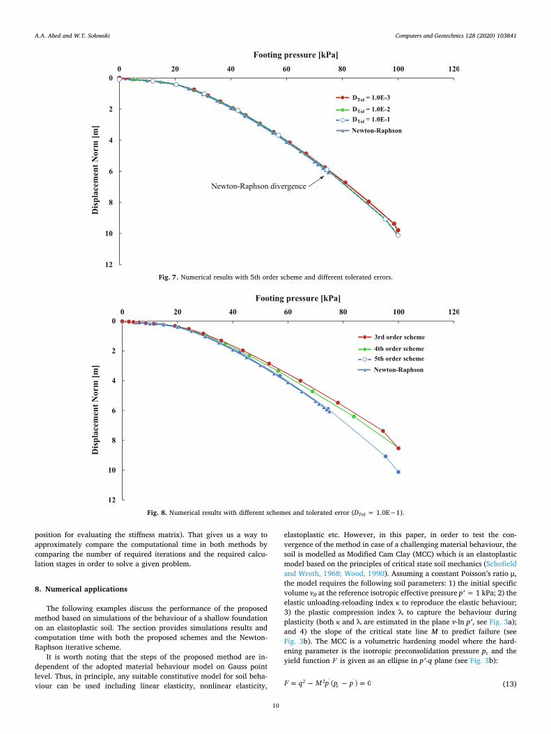
Fig. 7. Numerical results with 5th order scheme and different tolerated errors.

Fig. 8. Numerical results with different schemes and tolerated error (DTol = 1.0E−1).


10

where the isotropic pressure =p /3kk' ' and the deviatoric stress in-

variant = =s s sq p:ij ij ij ij ij32

' ' , with ij' being the effective Cauchy

stress tensor and ij is the Kronecker delta and i,j = 1,2,3. The modelassumes an associated flow rule.

In the case of overconsolidated clay, the initial isotropic pre-consolidation pressure is calculated based on the measured pre-over-burden pressure POP (the maximum vertical effective stress ever ex-perienced by the soil) and Eq. (13) yielding:

= × + ++

p POP M K KM K

[ (1 2 ) 9( 1) ]3 (1 2 )c

oNC

oNC

oNC

2 2 2

2 (14)

where KoNC is the coefficient of at-rest earth pressure as predicted by

MCC model for normally consolidated clay (Brinkgreve and Vermeer,1992):

+K M

M1.6 0.2

1oNC

(15)

The stress integration in case of MCC model can be carried out usingserval standard schemes including the explicit schemes with errorcontrol (Sloan, 1987; Sołowski and Gallipoli, 2010) and implicitschemes (Borja and Lee, 1990; Abed, 2008). Thebes code offers bothoptions to integrate MCC model, however in the following examplesonly the implicit scheme for the local stress integration is used.

8.1. Circular footing on Modified Cam Clay soil

The first example is an analysis of a circular shallow foundation. The1.0 m radius footing rests on a dry homogeneous slightly over-con-solidated clay with POP = 20 kPa. This POP value, based on Eqs. (14)and (15), leads to an initial isotropic overconsolidation pressure

=p 18.25c kPa. The unit weight of the clay is assumed to be 17.0 kN/m3

and the stresses were initialized with at rest soil pressure coefficient=K 0.5o . Table 8 lists the adopted MCC parameters in this analysis. The

footing applies a uniformly distributed stress of 100 kPa directly on the




11

soil in axisymmetric conditions, representing the case of a perfectlyflexible footing. The theoretical ultimate bearing capacity of the footingis around 110 kPa (Vesic, 1975). Fig. 4 shows the finite element modeland the problem geometry. The mesh consists of 2100 4-noded quad-rilateral finite elements with 4 stress integration points per element.Standard mechanical boundary conditions are applied to the problemboundaries with constrained horizontal deformations on the verticalboundaries and fully constrained deformations at the bottom boundary.The numerical analysis is carried out using the finite element codeThebes (Abed and Sołowski, 2017, 2019). Originally, the code used fullNewton-Raphson scheme to solve the finite element equations, whichwill be used here as a reference for comparison purposes. The 100 kPaexternal stress is applied as one loading increment, and then the au-tomatic scheme divided it into the appropriate sub-increments to satisfythe required accuracy using the desired order of the Runge-Kuttascheme. Automatic sub-incrementation is also used for the Newton-Raphson method to constrain the maximum relative error toITOL = 1.0E−3. It is worthwhile to mention that the Newton-Raphsonsub-incrementation follows similar steps to that in Table 7 with threemain differences: 1) The displacements in Step 2 are estimated usingNewton-Raphson iterations; 2) The “Error” estimation in phase (c) ofStep 2 bases on calculated forces instead of displacements where

=Error r f/i ext i, . Here ri is the norm of force residual (out-of-

balance) and fext i, is the applied external load at the current loadinglevel i and 3) the value of in the phase (d) of Step (2) is estimated as

= IError

Tol .

8.1.1. Discussion of the numerical resultsTables 9–11 report the numerical results of the analyses obtained

with a range of displacement error tolerance DTol and a range of Runge-Kutta schemes of different orders. The Tables give the number of re-quired sub-increments, the number of stages and the relative time withreference to tref - the time required by the 5th order scheme. Figs. 5–7graphically show the applied footing pressure versus the Euclidiannorm of displacement in the studied domain for the different methodsadopted in this study. Each graph includes the results using the Newton-Raphson method for the comparison purposes. For example Fig. 8,Fig. 9 and Fig. 10 illustrate the predictions of 3rd, 4th and 5th orderschemes with DTol = 1.0E−1, 1.0E−2 and 1.0E−3, respectively. Theresults show that for DTol = 1.0E−3, all Runge-Kutta schemes ap-proximated successfully the correct solution. However, the number ofthe required sub-increments to obtain the solution differs significantlyfrom one scheme to another. It is worth noting that in the case of the5th order scheme, the deviation from the correct solution is relativelysmall, no matter which tolerance is adopted. For this example, the fullNewton-Raphson algorithm diverged around the applied footing stress

Fig. 11. Sub-increment size variation in case of 5th order scheme with tolerated error (1.0E−3).

Fig. 12. The relative error in case of 5th order scheme with tolerated error (1.0E−3).


12

Fig. 13. Predictions of different available numerical codes for the vertical displacements under the centre of the footing.

Table 12Time and number of sub-increments required by the 5th order scheme with DTol = 1.0E−3 versus time and number of iterations required by full Newton-Raphsonmethod in case of normally consolidated clay.



Newton-Raphson 78 0 341 ≈ t1.25 ref(3) with divergence at 71 kPa

Fig. 14. Numerical results in case of normally consolidated clay.


13

of 75 kPa illustrating one of the significant merits of the new method,which always succeeded to complete the calculations and provide theresults without numerical difficulties. In addition, the 5th order schemeis considerably faster than the Newton-Raphson scheme as it succeededto compute the results for the full 100 kPa loading in about 25% fasterthan the time needed by the iterative scheme to reach 75 kPa loadingbefore diverging. That is confirmed by using the approximate assess-ment of the number of calculations based on count of the total numberof calculation stages and iterations. The 5th order scheme completedthe calculations with 108 calculation stages versus 131 iterations doneby the Newton Raphson scheme before it diverges and triggers con-tinuous unsuccessful attempts to converge by reducing consecutivelythe load increment size. Additionally, the Newton-Raphson schemecould easily reach 200 iterations if the iterative method would be ableto converge and compute the final results (corresponding to full loadincrement applied).

Table 9, Table 10, Table 11 and Fig. 8, Fig. 9, Fig. 10 illustrate theresults of the different schemes but with a similar tolerance. The graphsclearly show the significant differences in the required number of sub-increments (illustrated by dots) in each scheme to reach the prescribedaccuracy. It is also clear that the 5th order scheme is the most accurateand requires the lowest number of sub-increments which verifies thetheoretical expectations.

Fig. 11 shows the sub-increment sizes with loading for the case ofthe 5th order scheme and DTol = 1.0E−3. The graph illustrates thegeneral tendency of the error control scheme to accelerate the increaseof the load increment size as long as the load-displacement curve issmooth, and the slope is not changing dramatically (pure elasticity).Once the curve changes in a non-smooth manner (soil becomes plasticas stress reaches the preconsolidation pressure value, which is a non-smooth transition), the load increment size reduces in order to controlthe error. Once plastic behaviour is present, the load-displacementcurve becomes smooth again, the scheme starts accelerating and thestep size increases quickly again. Fig. 12 shows that the occurred re-lative error is kept below 1.0E−3 throughout the loading sequencewhich verifies the capability of the procedure to constrain the errorbelow the prescribed threshold.

8.1.2. Comparison to commercial codes resultsExactly the same problem was modelled using Plaxis2D (Brinkgreve

et al., 2016) and OptumG2 (Krabbenhoft et al., 2018), two well-es-tablished commercial software for finite element calculations in geo-technical applications. Fig. 13 depicts the results of the calculations interms of the predicted vertical displacements directly under the centrepoint of the footing (point A in Fig. 4). Plaxis could not advance furtherthan 60 kPa where the calculations stopped indicating soil collapse.Even after activating the arc-length control option, Plaxis code stilldiverges at that point. It is worth mentioning that Plaxis uses themodified Newton Raphson iterative scheme to solve the balanceequations. A similar observation applies to OptumG2 which shows evenearlier divergence around 50 kPa. The full Newton-Raphson method asimplemented in Thebes code diverged around 75 kPa while the newRunge-Kutta scheme succeeded to finish the calculations smoothly.These calculations demonstrate the potential of the new method to becompetitive if compared to the implicit iterative method.

8.2. Footing on normally consolidated (NC) clay

Table 12 and Fig. 14 report the results of the code predictions forthe same footing problem but with an overburden pressurePOP = 1.0 kPa to model a normally consolidated clay. The analysisinvolves the Newton-Raphson method and the 5th order explicitscheme. Similar observations to that in the previously discussed case ofhigher POP of 20 kPa (overconsolidated soil) apply here as well. Theanalysis run with the 5th order Runge-Kutta scheme completed suc-cessfully while the calculations with the iterative Newton Raphson

procedure failed under external stress of 71 kPa. In addition, the 5thorder scheme required 50 sub-increments and 300 calculations stages togo through the complete loading. The iterative scheme needed 341iterations to reach 71 kPa before the divergence. The actual relativetime needed by the Newton-Raphson method is again about 25% inexcess of the time needed by the 5th order scheme to carry out a similaranalysis. This example illustrates that for plasticity-dominant-problems,where the iterative procedures need an increasing number of iterationsto converge, the 5th order scheme possesses, besides the convergencemerits, competency with respect to the analysis efficiency and speed.

9. Conclusions

This paper introduced a new method to solve the load-displacementfinite element equations based on Runge-Kutta scheme. The method isimplemented with different local truncation errors up to 5th order.Additionally, the procedure includes a routine that automatically con-trols the load increment size to restrict the load path error within adesired range. The performance of the procedure is verified by solvingchallenging shallow foundation problems supported by an elastoplasticmaterial. The tackled numerical applications compared the proposedmethod with other common methods used for the solution, includingthe Newton-Raphson scheme and the arc-length method. The primaryfindings are: 1) in comparison to Newton Raphson iterative method, thenew explicit method proved to be not only more stable but also com-petitive with respect to the speed of solution especially when the 5thorder Runge-Kutta scheme is employed; 2) the convergence of theproposed scheme is assured even in highly nonlinear problems, whilethe other schemes fail; 3) the presented procedure is universal, and theproposed method can be extended to even higher-order Runge-Kuttaschemes easily. Finally, more research is needed to check whether thebenefits of the proposed method are also present in other highly non-linear problems. For example, those may involve coupled multi-physicswhere numerical instability and divergence are relatively common, forinstance in the case of coupled thermo-hydro-mechanical-chemical(THMC) problems.

CRediT authorship contribution statement

Ayman A. Abed: Methodology, Software, Validation, Writing -original draft, Visualization.Wojciech T. Sołowski: Conceptualization,Supervision, Writing - review & editing.

Declaration of Competing Interest

The authors declare that they have no known competing financialinterests or personal relationships that could have appeared to influ-ence the work reported in this paper.

Acknowledgement

The authors would like to acknowledge gratefully that the presentedresearch has been funded by the Civil Engineering Department’s basicresearch fund at Aalto University. The authors would also like to ac-knowledge inspiring discussions with Prof. Kristian Krabbenhoft(University of Liverpool), which led to the initiation of this research.

References

Abbo, A.J., Sloan, S.W., 1996. An automatic load stepping algorithm with error control.Int. J. Numer. Methods Eng. 39, 1737–1759.

Abed, A., 2008. Numerical modeling of expansive soil behavior. Instituts für Geotechnik(IGS).

Abed, A., Sołowski, W., 2017. A study on how to couple thermo-hydro-mechanical be-haviour of unsaturated soils: Physical equations, numerical implementation and ex-amples. Comput. Geotech. 92, 132–155.

Abed, A.A., Sołowski, W.T., 2019. Applications of the new thermo-hydro-mechanical-


14

http://refhub.elsevier.com/S0266-352X(20)30404-3/h0005







chemical coupled code ‘Thebes’. Environ. Geotech. https://doi.org/10.1680/jenge.18.00083.

Avriel, M., 2003. Nonlinear programming: analysis and methods. Courier Corporation.Bathe, K.-J., 2006. Finite element procedures. Klaus-Jurgen Bathe.Bischof, C., Carle, A., Corliss, G., Griewank, A., Hovland, P., 1992. ADIFOR–generating

derivative codes from Fortran programs. Sci. Program 1, 11–29.Bischof, C., Khademi, P., Mauer, A., Carle, A., 1996. ADIFOR 2.0: Automatic differ-

entiation of Fortran 77 programs. IEEE Comput. Sci. Eng. 3, 18–32.Borja, R.I., Lee, S.R., 1990. Cam-clay plasticity, part 1: implicit integration of elasto-

plastic constitutive relations. Comput. ApplMechEng. 78, 49–72.Brinkgreve, R., Kumarswamy, S., Swolfs, W., 2016. PLAXIS 2016. Plaxis bv, Delft.Brinkgreve, R.B.J., Vermeer, A., 1992. On the use of Cam-Clay models. Symp. Numer.

Models Geomech. Balkema Rotterdam Neth.Broyden, C.G., 1965. A class of methods for solving nonlinear simultaneous equations.

Math. Comput. 19, 577–593.Crisfield, M.A., 1983. An arc-length method including line searches and accelerations. Int.

J. Numer. Methods Eng. 19, 1269–1289.Gens, A., Potts, D.M., 1988. Critical state models in computational geomechanics. Eng.

Comput. 5, 178–197.Griewank, A., Walther, A., 2008. Evaluating derivatives: principles and techniques of

algorithmic differentiation, vol. 105. Siam.Gustafsson, K., 1992. Control of error and convergence in ODE solvers.Krabbenhoft, K., Lymain, A., Krabbenhoft, J., 2018. OptumG2. Optum Comput. Eng.Laitinen, M., 2013. Numerrin 4.0 Manual. Numerola Oy.Lee, H.J., Schiesser, W.E., 2003. Ordinary and partial differential equation routines in C,

C++, Fortran, Java, Maple, and Matlab. Chapman and Hall/CRC.Matthies, H., Strang, G., 1979. The solution of nonlinear finite element equations. Int. J.

Numer. Methods Eng. 14, 1613–1626.Mitusch, S.K., 2018. An Algorithmic Differentiation Tool for FEniCS.Potts, D.M., Ganendra, D., 1992. A comparison of solution strategies for non-linear finite

element analysis of geotechnical problems. Proc. 3rd Int. Conf. Comput. Plast. Barc.803–814.

Rothe, S., Hartmann, S., 2015. Automatic differentiation for stress and consistent tangentcomputation. Arch. Appl. Mech. 85, 1103–1125.

Schofield, A., Wroth, P., 1968. Critical state soil mechanics.Sheng, D., Sloan, S.W., 2001. Load stepping schemes for critical state models. Int. J.

Numer. Methods Eng. 50, 67–93.Sloan, S.W., 1987. Substepping schemes for the numerical integration of elastoplastic

stress–strain relations. Int. J. Numer. Methods Eng. 24, 893–911.Sloan, S.W., Abbo, A.J., Sheng, D., 2001. Refined explicit integration of elastoplastic

models with automatic error control. EngComput. 18, 121–194.Smith, I.M., Griffiths, D.V., Margetts, L., 2013. Programming the finite element method.

John Wiley & Sons.Sołowski, W.T., Gallipoli, D., 2010. Explicit stress integration with error control for the

Barcelona Basic Model: Part I: Algorithms formulations. ComputGeotech. 37, 59–67.Tijskens, E., Roose, D., Ramon, H., De Baerdemaeker, J., 2002. Automatic differentiation

for solving nonlinear partial differential equations: an efficient operator overloadingapproach. Numer. Algorithms 30, 259–301.

Vesic, A.S., 1975. Bearing capacity of shallow foundations. Found Eng. Handb.Wood, D.M., 1990. Soil behaviour and critical state soil mechanics. Cambridge University

Press.Zwicke, F., Knechtges, P., Behr, M., Elgeti, S., 2016. Automatic implementation of ma-

terial laws: Jacobian calculation in a finite element code with TAPENADE. Comput.Math. Appl. 72, 2808–2822.


15

https://doi.org/10.1680/jenge.18.00083

https://doi.org/10.1680/jenge.18.00083
















































Documents

Finite element method algorithm for geotechnical