Finite Element Analysis of Geotechnical Rehabilitation Works

地盤構造物の修復技術に関する有限要素解析

Annamaria Cividini *, Giorgio Borgonovo** and Giancarlo Gioda*

* Department of Structural Engineering, Politecnico di Milano Piazza Leonardo da Vinci 32, 20133 Milano, Italy

(e-mail: annamaria.cividini@polimi.it)

** Consulting Engineer Via Renato Serra 6, 20148 Milano, Italy

TECHNICAL PAPER（技術報告）

要約

有限要素法は、多くの工学の現場で応力解析に使われ、設計者が構造物の寸法や力学

挙動を設定するのに役立っている。 しかしながら、これらのやり方は数値解析の持つ潜在能力を十分に引き出していると

はいえない。実際、数値解析は応力解析における標準的な手計算や簡易手法を縛るだけ

ということになっている。 有限要素法は、構造物の数値モデルを開発するに際して様々な条件下における解を与

えることができる。このことによって、構造物の挙動をより深く理解し、設計や与えら

れた構成則、関連したパラメータなどを改良することが可能となろう。 原位置測定の結果に対する確定論的あるいは確率論的な逆解析は、地盤工学における

数値解析モデルのこのような“柔軟な”利用の良い例である。 本報告では、このような利用法を地盤構造物の修復作業に適用した例を示す。数値モ

デルは既存の情報（当初の寸法、力学特性、等）に基づいて開発されており、これらの

パラメータは可能な限り原位置測定の結果に従って修正される。 このキャリブレーションを経て数値モデルは、修復デザイナーによって提案される各

種の予備解析に適用される。キャリブレーションの結果は、可能な技術的選択肢を与え

る基礎になっており、最も適切な手法を選択する有益な補助手段となっている。 本報告では、数値解析法の２例の適用例を示す。これらは、それぞれ、橋脚のアンダ

ーピニングと斜面のゆっくりとした時間依存変形挙動の安定化に適用したものである。 著者紹介：Gioda 博士と Cividini 博士はご夫婦で同じ大学(ミラノ工科大学)の同じ学科で

教授職を務める魅力的なカップルであり、逆解析の先駆的な研究や地盤構造物の数値解

析で世界的に高名な研究者です。ミラノは、大理石造の大聖堂やスフォルツァ城、ミケ

ランジェロの最後の晩餐などの古い文化と、銀行業やファッションを始めとした現代産

業が調和した北イタリアの中心都市です。本報告にあるように、古い構造物の修復作業

はイタリアの大きな課題であり、日本の技術者とも交流が図られるよう期待されます。 （文責：市川康明）

1

1. INTRODUCTION

The finite element method is frequently used in engineering practice for solving stress analysis

problems the characteristics of which (e.g. dimensions, mechanical behaviour, etc.) have been a

priori chosen by the designer.

It should be observed, however, that this approach does not fully exploit the potentials of the

numerical method. In fact it restricts it to the same role of standard hand-calculations or simplified

methods for stress analysis.

The finite element method can be also used, in fact, to develop a numerical model of the struc-

ture that permits predicting its answer to a variety of different conditions. This leads to a deeper

understanding of its behaviour and to possible improvements of the design, of the adopted constitu-

tive laws, of their relevant parameters, etc.

The deterministic and probabilistic approaches to the back analysis of in situ measurements rep-

resent a notable example of this “flexible” use of numerical models in geotechnical engineering

[1,2,3,4].

Here this approach is applied to the design of geotechnical rehabilitation works. The numerical

model is developed on the basis of the available information (original geometry, mechanical prop-

erties, etc.) and, if possible, its parameters are calibrated through the back analysis of the measure-

ments performed in situ during time.

Upon its calibration the numerical model is then applied to the analysis of the provisions sug-

gested by the designer for rehabilitation. The results of calculations provide a basis for the com-

parative evaluation of possible alternative techniques and represent a valuable help in choosing the

most convenient among them.

This use of the numerical analysis is illustrated here through two case histories. They are re-

lated, respectively, to the underpinning of a bridge pier and to the stabilization of a slope undergo-

ing a slow time dependent movement.

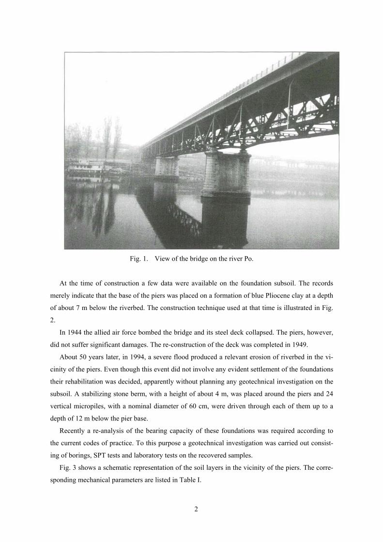
2. A BRIDGE ON THE RIVER PO

The first problem here discussed concerns the piers of a relatively old bridge on the river Po of the

Italian state road named Emilia connecting Milan to Bologna [5].

The bridge was completed in 1904. A steel truss structure forms the portion of its deck crossing

the river. Two concrete piers are located within the riverbed and are covered with stones for protec-

tion from the erosion of water. They reach a height of about 22 m from the riverbed (Fig. 1) and

have a 12 m x 4 m rectangular cross section with rounded corners.

2

Fig. 1. View of the bridge on the river Po.

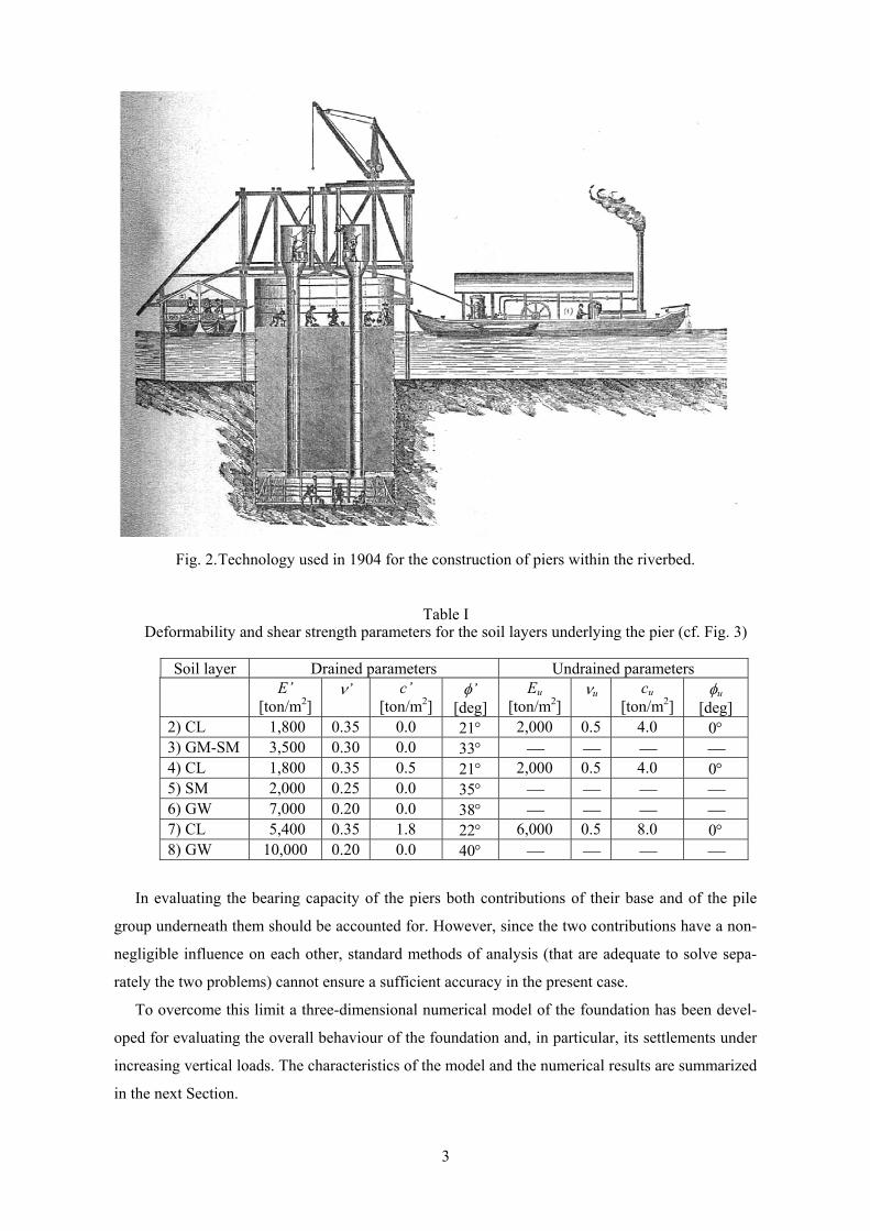
At the time of construction a few data were available on the foundation subsoil. The records

merely indicate that the base of the piers was placed on a formation of blue Pliocene clay at a depth

of about 7 m below the riverbed. The construction technique used at that time is illustrated in Fig.

2.

In 1944 the allied air force bombed the bridge and its steel deck collapsed. The piers, however,

did not suffer significant damages. The re-construction of the deck was completed in 1949.

About 50 years later, in 1994, a severe flood produced a relevant erosion of riverbed in the vi-

cinity of the piers. Even though this event did not involve any evident settlement of the foundations

their rehabilitation was decided, apparently without planning any geotechnical investigation on the

subsoil. A stabilizing stone berm, with a height of about 4 m, was placed around the piers and 24

vertical micropiles, with a nominal diameter of 60 cm, were driven through each of them up to a

depth of 12 m below the pier base.

Recently a re-analysis of the bearing capacity of these foundations was required according to

the current codes of practice. To this purpose a geotechnical investigation was carried out consist-

ing of borings, SPT tests and laboratory tests on the recovered samples.

Fig. 3 shows a schematic representation of the soil layers in the vicinity of the piers. The corre-

sponding mechanical parameters are listed in Table I.

3

Fig. 2. Technology used in 1904 for the construction of piers within the riverbed.

Table I Deformability and shear strength parameters for the soil layers underlying the pier (cf. Fig. 3)

Soil layer Drained parameters Undrained parameters

E’ [ton/m2]

ν’ c’ [ton/m2]

φ’ [deg]

Eu [ton/m2]

νu cu [ton/m2]

φu [deg]

2) CL 1,800 0.35 0.0 21° 2,000 0.5 4.0 0° 3) GM-SM 3,500 0.30 0.0 33° 4) CL 1,800 0.35 0.5 21° 2,000 0.5 4.0 0° 5) SM 2,000 0.25 0.0 35° 6) GW 7,000 0.20 0.0 38° 7) CL 5,400 0.35 1.8 22° 6,000 0.5 8.0 0° 8) GW 10,000 0.20 0.0 40°

In evaluating the bearing capacity of the piers both contributions of their base and of the pile

group underneath them should be accounted for. However, since the two contributions have a non-

negligible influence on each other, standard methods of analysis (that are adequate to solve sepa-

rately the two problems) cannot ensure a sufficient accuracy in the present case.

To overcome this limit a three-dimensional numerical model of the foundation has been devel-

oped for evaluating the overall behaviour of the foundation and, in particular, its settlements under

increasing vertical loads. The characteristics of the model and the numerical results are summarized

in the next Section.

4

Fig. 3. Schematic representation of the soil layers underneath the pier.

3. ANALYSIS OF THE BRIDGE FOUNDATION

A 3D finite element model, consisting of 8 node “brick” elements, was prepared to properly ac-

count for both interactions between the piles and between the piles and the pier base. Because of

the problem symmetry the discretization was extended only to one quarter of the pile group. The

calculations were carried assuming an elastic-perfectly plastic behaviour governed by Mohr-

Coulomb yield condition and neglecting the volume changes due to plastic dilatation.

A plane view of the base of the pier and a detail of the corresponding mesh are shown in Fig 4.

The entire three-dimensional mesh is depicted in Fig. 5. The top of the mesh coincides with the

base of the foundation and its bottom is located 40 m below it. The stabilizing berm and the soil

above the base were introduced as dead loads neglecting the lateral skin resistance of the pier. For

an accurate evaluation of the base resistance of the piles the mesh has been refined in the vicinity of

their tips.

5

Fig. 4. Distribution of piles on the pier base and detail of the finite element grid.

The evaluation of the load-settlement diagram of the pier (cf. Figs. 6 and 7) was subdivided into

a series of steps related to the different states of the foundation during its life. First the in situ stress

state in the soil mass prior to the bridge construction was estimated subjecting the 3D mesh to the

submerged own weight of soil. This analysis was performed in elastic regime adopting for all lay-

ers a value of Poisson ratio that corresponds to a coefficient of earth pressure at rest equal to 0.5.

The second step involved the application of the own weights of the pier, of the relevant parts of

the deck and of the stabilizing berm. This calculation was carried out in elasto-plastic regime

adopting the drained parameters for the cohesive layers.

This step led to the initial conditions from which the increase of the load on the pier was simu-

lated under different conditions, namely: a) no piles, b) 12 m long piles and, c) 15 m long piles. In

order to evaluate the short-term and the long-term behaviour of the foundation, the analyses were

repeated considering both drained and undrained parameters for the cohesive layers.

The results of calculations are summarized through the load-settlement diagrams in Figs. 6 and

7. It can be observed that under the permanent load the long-term settlement of the foundation is

relatively small. In fact, no appreciable settlements were reported during the construction of the

bridge and during the subsequent decades.

6

Fig. 5. Three-dimensional finite element grid.

Fig. 6. Load-settlement response of the pier in undrained conditions.

7

Fig. 7. Load-settlement response of the pier in drained conditions.

Beside the trivial observation that the undrained settlements are appreciably smaller than the

drained ones, the two sets of diagrams indicates that the piles with length of 12 m do not apprecia-

bly increase the overall stiffness of the foundation. Their limited influence depends on the fact that

they cross layers of relatively soft soils and barely reach a deeper layer of gravel.

Based on this observation, the analyses where repeated increasing the pile length to 15 m, so

that they penetrate well inside the mentioned gravel layer. The consequent marked increase of the

overall stiffness of the foundation is clearly shown in Figs. 6 and 7 and in Table II that reports the

variation of the tangent stiffness of the foundation (for a load increase starting from the permanent

load level) with increasing pile length.

Table II Variation of the overall stiffness of the foundation with the pile length

Foundation Stiffness

[ton/cm] Pile Length

L [m] Drained Undrained

0. 131.0 138.0 12. 143.0 157.0 15. 947.2 947.5

It can be observed that in the cases without piles and with 12 m long piles the drained stiffness

is lower than the undrained one. This means that the cohesive layers have a non-negligible influ-

ence on the foundation behaviour. On the contrary, the same stiffness was obtained in undrained

and drained conditions with 15 m long piles. In this case, in fact, the piles transmit the load in-

8

crease exceeding the permanent loads almost completely to the gravel layer and the influence of the

intermediate soft soils becomes negligible.

The contour lines of the square root of the second invariant of the deviatoric plastic strains in

Figs. 8, 9 and 10 provide a further insight into the influence of piles. These figures refer to the

drained results for an applied load equal to three times the permanent load and represent the men-

tioned contour lines on a vertical section through the foundation centreline. A large load level was

adopted to emphasize the spreading of the plastic zone.

In the case without piles (Fig. 8) the plastic zone involves the entire soil mass underneath the

foundation up to the gravel layer. The large plastic strains clearly indicate that the foundation is

close to collapse.

A similar condition is reached for the case with 12 m piles (Fig. 9). In this case the deep founda-

tion does not appreciably constrain the spreading of plasticity and the consequent displacements

(cf. Fig. 7).

Fig. 8. Drained analysis of the foundation without piles: contour lines of the square root of the second invariant of the deviatoric plastic strains γ* on the vertical section through the foundation centreline. (The applied load is equal to the permanent load multiplied by 3; the contour lines in the vicinity of the foundations are not shown).

9

Fig. 9. Contour lines of γ* for the pier with 12 m long piles (other characteristics as in Fig 8).

Fig. 10. Contour lines of γ* for the pier with 15 m long piles (other characteristics as in Fig 8).

10

However, a substantially different state is obtained for the 15 m piles that penetrate within the

gravel layer (Fig. 10). No plastic strains develop in the soil among the piles and quite limited plas-

tic strains are evaluated at the base of the group within the gravel layer. This implies that the base

bearing capacity of the pile group has not been reached yet.

Only the lateral skin resistance of the group has been attained. In fact, the permanent strains are

concentrated in a relatively thin portion of soil facing the external surface of the pile group.

It seems possible to conclude that, even though the 12 m long piles driven in 1994 increase the

bearing capacity of the pier, they have a limited influence on its overall behaviour under increasing

vertical loads.

If slightly longer (15 m) piles would have been used perhaps their effects could have been more

pronounced, obtaining a substantial increase of the overall stiffness of the foundation.

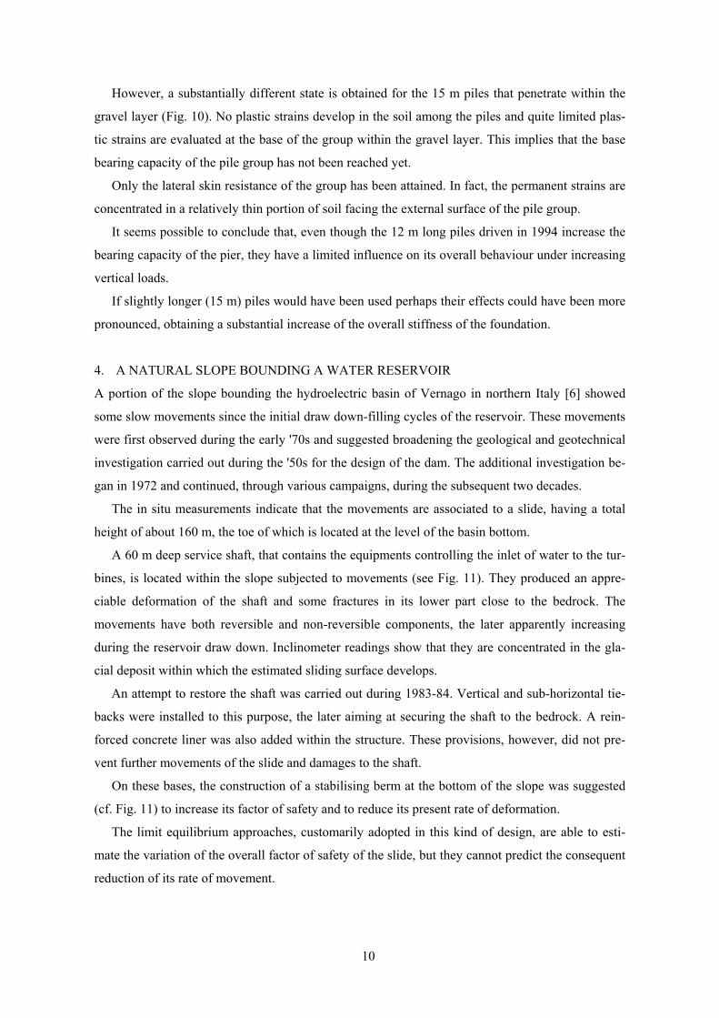
4. A NATURAL SLOPE BOUNDING A WATER RESERVOIR

A portion of the slope bounding the hydroelectric basin of Vernago in northern Italy [6] showed

some slow movements since the initial draw down-filling cycles of the reservoir. These movements

were first observed during the early '70s and suggested broadening the geological and geotechnical

investigation carried out during the '50s for the design of the dam. The additional investigation be-

gan in 1972 and continued, through various campaigns, during the subsequent two decades.

The in situ measurements indicate that the movements are associated to a slide, having a total

height of about 160 m, the toe of which is located at the level of the basin bottom.

A 60 m deep service shaft, that contains the equipments controlling the inlet of water to the tur-

bines, is located within the slope subjected to movements (see Fig. 11). They produced an appre-

ciable deformation of the shaft and some fractures in its lower part close to the bedrock. The

movements have both reversible and non-reversible components, the later apparently increasing

during the reservoir draw down. Inclinometer readings show that they are concentrated in the gla-

cial deposit within which the estimated sliding surface develops.

An attempt to restore the shaft was carried out during 1983-84. Vertical and sub-horizontal tie-

backs were installed to this purpose, the later aiming at securing the shaft to the bedrock. A rein-

forced concrete liner was also added within the structure. These provisions, however, did not pre-

vent further movements of the slide and damages to the shaft.

On these bases, the construction of a stabilising berm at the bottom of the slope was suggested

(cf. Fig. 11) to increase its factor of safety and to reduce its present rate of deformation.

The limit equilibrium approaches, customarily adopted in this kind of design, are able to esti-

mate the variation of the overall factor of safety of the slide, but they cannot predict the consequent

reduction of its rate of movement.

11

Fig. 11. Vertical section of the slope with the service shaft and the suggested stabilizing berm.

An attempt to evaluate this important design parameter has been based on a series of non-linear,

plane strain, finite element analyses adopting two alternative material models, namely: a visco-

plastic constitutive law and an elasto-plastic law allowing for strain softening effects. In both cases

the driving forces causing the deformation of the slope were related to the pore pressure changes

taking place during the reservoir rising and draw down.

For sake of briefness, only the strain-softening finite element model is described here. Its results

provided some insight into the physical mechanisms governing the time dependent deformation of

the slide and led to an apparently reliable estimation of the slope behaviour after the construction of

the berm.

5. NUMERICAL MODEL OF THE SLIDE

As previously observed, the incremental displacements of the slide are related to the annual cycles

of the reservoir. The diagrams in Fig. 12 show the variation with time of the reservoir level and of

the horizontal displacement of the top and bottom of the slide calculated from the inclinometer

readings.

It can be observed that the increase of the water level during filling does not induce appreciable

irreversible displacements. On the contrary, they become significant during draw down and tend to

stabilise only after the reservoir has reached its minimum level.

12

Fig. 12. Variation with time of the water level within the reservoir and of the horizontal displace-ment of the top and bottom of the slide calculated from the inclinometer measurements.

This indicates that the slide is substantially stable during filling and, hence, that its instability

cannot be related solely to the buoyancy effects induced by the rise of the water table within the

slope. It seems therefore reasonable to assume that the observed movements depend on the seepage

forces developing within the slide when the water level in the reservoir is lowered.

It should be also considered that, being the mechanical behaviour of the soil deposits markedly

non-linear, the observed deformation is influenced by the state of stress initially present in the

slope prior to the initiation of the reservoir cycles.

The above observations suggest that the numerical model of the slide should be based on a

proper non-linear constitutive law for the relevant materials and should take into account the initial

stress state within the slope and the effects of buoyancy and seepage.

A correct evaluation of the initial stress state of the slide would require a detailed finite element

simulation of its geological formation process. This, however, is not an easy task due to the diffi-

culty in defining the characteristics of this process.

Based on previous experience [7] the initial stress distribution was approximated by modelling

the deposition of the slope in a number of subsequent steps. Each of them requires an elasto-plastic

analysis of the "active" part of the mesh subjected only to the own weight of the zone added during

the current step.

13

This procedure was applied to the mesh in Fig. 13 subdividing the process in about 50 steps. At

the end of these analyses the sought distribution of initial effective stresses was obtained by apply-

ing the buoyancy forces that correspond to the water table located at the bottom of the reservoir.

The calculations described in the following were carried out in plane strain regime. The mesh

was prepared taking into account the shape and location of the sliding surface suggested by the in

situ measurements. The elements in the sliding zone have an almost constant size to limit the influ-

ence of the discretization on the results of the strain softening analyses [8].

Fig. 13. Plane strain finite element mesh of the slope (1221 quadrilateral, four node, isoparametric elements and 1256 nodes).

An uncoupled approach was adopted to evaluate the buoyancy and seepage forces acting on the

soil skeleton. It was in fact considered that the deformation of the skeleton, having a relatively

large granular fraction, could not induce a relevant variation of pore pressure with respect to the

distribution associated to the seepage flow. Consequently a coupled, or consolidation, analysis did

not seem necessary for the problem at hand.

On this basis, the nodal pore pressures were first evaluated through a finite element seepage cal-

culation adopting the same mesh used also for the stress analyses. Then, the nodal forces equiva-

lent, in the finite element sense, to the calculated pore pressures were determined and introduced as

external loads in the stress analysis of the slide.

In general terms the nodal pore pressures developing during the reservoir cycles should be

evaluated through unconfined, transient seepage analyses (see. e.g. [9]). This, however, would re-

quire a detailed description of the distributions of the hydraulic conductivity and void ratio within

14

the slope. Since this information is not available with a sufficient accuracy, the seepage analyses

were limited to confined, steady state conditions.

It was assumed, in particular, that during filling the water table within the slope is horizontal

and coincides at any instant of time with the level of the reservoir (cf. Fig. 14). Under this assump-

tion no seepage takes place and only the buoyancy forces should be accounted for. These forces

were evaluated in the conditions corresponding to the minimum and maximum water levels in the

reservoir, represented by lines I and II in Fig. 14. Then the difference between them was gradually

applied to the slope during a time span coinciding with the average time required by filling.

Fig. 14. Simplified variation of the phreatic surface assumed during the reservoir filling

The draw down process was simulated taking into account that the granular deposits close to the

slope surface have a relatively high permeability and that the drainage of water takes place from

them at a rate comparable to that of the lowering process within the reservoir. Consequently, during

draw down the phreatic level within these shallow deposits should approximately coincide with the

reservoir level.

On the contrary, since the deeper layers have a relatively low coefficient of hydraulic

conductivity, a certain delay is possible between the lowering processes of the water table within

them and in the reservoir.

On this basis a scheme for the draw down process was adopted (cf. Fig. 15) in which the “in-

clined” portion of the phreatic surface coincides with the lower boundary of the shallow deposits.

The lowering process was simulated through a series of confined steady state analyses. The seepage

forces corresponding to the steps in Fig. 15 were applied in sequence, gradually varying them with

time, in order to simulate the lowering of the water table from lines II to V.

15

Fig. 15. Simplified variation of the phreatic surface assumed during the reservoir draw down

6. ANALYSIS OF THE SLIDE

The shear strength parameters derived from the available geological and geotechnical data are re-

ported in Table III with reference to the various layers depicted in Fig. 11.

As to the elastic parameters, their characterization is not straightforward since the geotechnical

and geological investigation show an appreciable scatter in their values. In addition, a non-

negligible difference exists between the elastic moduli derived from the geophysical survey, from

in the situ tests and from the laboratory tests.

To overcome this drawback, a first approximation of the elastic parameters was derived from

the geotechnical data, then their values were refined through the back analysis of the inclinometer

measurements.

The non-reversible part of the slope displacements was eliminated before performing the back

analysis since the sought elastic parameters govern only its reversible response. This was obtained

by subtracting the displacement of the bottom of the shaft to those recorded along its height. These

relative displacements, that do not show a substantial increase with time, were used as input data of

the back analysis.

The comparison between the reversible part of the measured increments of displacements be-

tween the top and bottom of the slide and the corresponding numerical results, based on the back

analyzed elastic constants (cf. Table III), is shown in Fig. 16. These results refer to one filling-draw

down cycle of the reservoir

16

Table III Elastic and shear strength parameters for slope in Fig. 11.

Layer E’

[ton/m2] ν’ c’

[ton/m2] φ’

[deg] Talus 8.0⋅104 0.3 2. 36°

Glacial deposit 8.0⋅104 0.3 6. 35° Alluvial deposit 5.2⋅104 0.3 2. 33°

Deposit with organic content

2.0⋅104 0.3 2. 33°

Bedrock 4.0⋅106 0.3 40. 40°

Fig. 16. Reversible part of the horizontal displacements of the top of the slide calculated from the inclinometer measurements and results of the linear analysis based on the back calculated elastic constants.

To allow for the numerical simulation of the downward movement of the slide it was consid-

ered that the deformation developing within its failure zone could produce a loss of the shear

strength of the involved materials. This hypothesis leads to the use of a strain softening constitutive

law in the elasto-plastic calculations.

A key point in using such a law concerns the choice of the ratios between residual (cr, φr) and

peak (cp, φp) values of the effective shear strength parameter. Unfortunately, the available geotech-

nical data were not sufficient with this respect.

It should be also considered that, if a limited reduction from peak to residual parameters is

adopted, the permanent deformation would stabilise after a few cycles. On the other hand, if the re-

17

duction is too pronounced, a general collapse of the slope could occur during the initial filling-

draw down cycles. In these conditions it seemed advisable to perform a parametric study, based on a series of strain

softening analyses, to quantitatively assess the influence of the ratio between residual and peak

shear strength parameters on the numerically evaluated behaviour of the slope.

In these analyses a linear variation of the strength parameters with increasing deviatoric plastic

strains was assumed, as depicted in Fig. 17. The adopted finite element procedure was described in

[10]. Note that the shear strength parameters in Table III characterize the peak failure condition.

Fig. 17. Adopted variation of the shear strength parameters with increasing square root of the sec-ond invariant of deviatoric plastic strains γ*.

The first part of the parametric study was limited to one filling of the reservoir and did not con-

sider the stabilising berm. Different values of the ratios αc=cr/cp and αφ=tanφr/tanφp where adopted

for each analysis in the range between 0 and 1. They were kept constant for all materials in the

slide.

The results of these calculations are summarised in Fig. 18. The overall collapse of the slope

develops during filling (zone C) for exceedingly small values of the residual strength. Larger val-

ues produce plastic strains (zone B), but do not induce collapse. Finally, further increases of αc and

αφ lead to an elastic behaviour of the slope (zone A).

Quite obviously, to model the actual behaviour of the slope the parameters αc and αφ should not

correspond to points within zone C. In fact they should correspond to points on or above the line

separating zones C and B.

18

Fig. 18. Influence of the ratios αc and αφ between residual and peak shear strength parameters on the numerically evaluated behavior of the slope during the reservoir filling (A: overall elastic behavior; B: elastic-plastic behavior; C: collapse).

A second series of softening analyses was performed that simulate one filling-draw down cycle

of the reservoir. Also in this case different values of αc and αφ were used in each calculation, keep-

ing the corresponding points within zones B or A of Fig. 18.

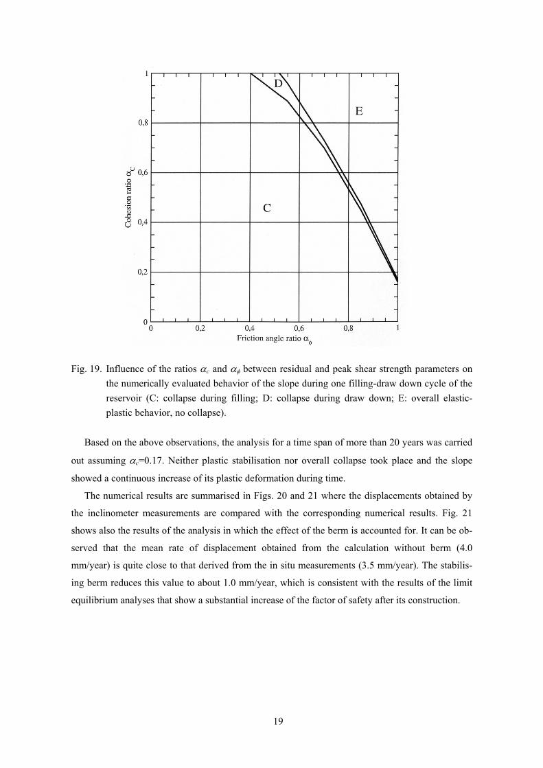
The results of this second parametric study are reported in Fig. 19. Here zone C coincides with

that in Fig. 18 and corresponds to the collapse of the slope during filling. Zones D and E corre-

spond, respectively, to the collapse during draw down and to the development of plastic deforma-

tion during draw down, but without reaching collapse.

Note that the behaviour of the slope during draw down is always in the plastic range (zone E),

even when no softening effects are introduced, i.e. when αc = αφ = 1.

From these results it appears that the values αc and αφ to be adopted in a cyclic analysis should

belong to zone E in Fig. 19, otherwise collapse would occur during the first filling (zone C) or dur-

ing the first draw down (zone D).

A unit value of αφ can be assumed since, as previously observed, the available geotechnical data

do not indicate a substantial reduction of the friction angle with increasing strains. As to αc, Fig. 19

shows that when αφ=1 the limit values of αc for which collapse occurs during the first filling or

during the first draw down almost coincide with each other, and that they are slightly smaller than

0.17.

19

Fig. 19. Influence of the ratios αc and αφ between residual and peak shear strength parameters on the numerically evaluated behavior of the slope during one filling-draw down cycle of the reservoir (C: collapse during filling; D: collapse during draw down; E: overall elastic-plastic behavior, no collapse).

Based on the above observations, the analysis for a time span of more than 20 years was carried

out assuming αc=0.17. Neither plastic stabilisation nor overall collapse took place and the slope

showed a continuous increase of its plastic deformation during time.

The numerical results are summarised in Figs. 20 and 21 where the displacements obtained by

the inclinometer measurements are compared with the corresponding numerical results. Fig. 21

shows also the results of the analysis in which the effect of the berm is accounted for. It can be ob-

served that the mean rate of displacement obtained from the calculation without berm (4.0

mm/year) is quite close to that derived from the in situ measurements (3.5 mm/year). The stabilis-

ing berm reduces this value to about 1.0 mm/year, which is consistent with the results of the limit

equilibrium analyses that show a substantial increase of the factor of safety after its construction.

20

Fig. 20. Incremental horizontal displacements measured at the service during 15 years and corre-sponding numerical results.

Fig. 21. Measured and calculated horizontal displacements of the top of the slide and variation of the water level in the reservoir during time. The numerical results refer to both cases with and without the stabilizing berm.

21

7. CONCLUDING REMARKS

The application of the finite element method for modelling the rehabilitation of pre-existing geo-

technical works has been discussed with reference to the underpinning of a bridge pier and to the

stabilization of a slope undergoing a time dependent movement.

In both cases the numerical model has been developed on the basis of the available information

on geometry, material properties, etc. For the slope problem, the material parameters were subse-

quently refined through the back analysis of the displacements measured in situ during time.

The calibrated numerical models were then applied to the analysis of the examined structures in

their original conditions and after completion of their rehabilitation.

The results permit a quantitative evaluation of the effectiveness of the suggested rehabilitation.

For instance, for the pier problem it turned out that the length of the installed piles does not guaran-

tee a significant increase of the overall stiffness of the foundation.

It can be concluded that the described approach could help the designer in assessing the effec-

tiveness of the chosen rehabilitation method or for identifying the most convenient method among

various possible alternatives.

REFERENCES

[1] Sakurai S., Takeuchi K. (1983): Back analysis of measured displacements of tunnels. Rock Mechanics and Rock Engineering, 16, 173-180.

[2] Asaoka A., Matsuo M. (1984): An inverse problem approach to the prediction of multi-dimensional consolidation behaviour. Soils and Fondations, 24(1), 49-62.

[3] Ichikawa Y., Ohkami T. (1992): A parameter identification procedure as a dual boundary con-trol problem for linear elastic materials. Soils and Foundations, 32(2), 35-44.

[4] Murakami A., Hasegawa T. (1993): Application of Kalman filtering to inverse problems. Theoretical and Applied Mechanics, 43, 3-14.

[5] Malerba P.G. (2000): Il Ponte sul Po di Piacenza. In “Infrastrutture di Trasporto nel Sistema Metropolitano tra la Regione Emilia e la Regione Lombardia”, Technical paper, Fondazione di Piacenza e Vigevano.

[6] Gioda G., Borgonovo G., (2004): Finite element modelling of the time-dependent deformation of a slope bounding a hydroelectric reservoir. To appear in International Journal of Geome-chanics.

[7] Forlati F., Gioda G., Scavia C. (2001): Finite element analysis of a deep-seated slope deforma-tion. Rock Mechanics and Rock Engineering, 34(2), 135-159.

[8] Pietruszczak S., Mroz Z. (1981): Finite element analysis of deformation of strain softening materials. Int.J.Numer.Meth.Engng., 17, 327-334.

[9] Cividini A., Gioda, G. (1989): On the variable mesh finite element solution of unconfined seepage problems. Geotechnique, 39(2),.251-267.

[10] Cividini A., Gioda G. (1992): Finite element analysis of direct shear tests on stiff clays, Int.J.Numer.Analyt.Meth.Geomechanics, 16, 869-886.