Embed Size (px)
Citation preview
Financial Lumpiness and Investment
Santiago Bazdresch∗
Yale University
November 2005
Abstract
This paper shows that non-convex costs of financial adjustment areimportant for rationalizing observed investment and financing choices offirms. Using the COMPUSTAT database it first shows firm’s financingactivity, like investment, can be characterized as lumpy. Financial adjust-ments are infrequent and a small fraction of observations account for mostof the external financing activity. The paper then presents a model whichshows that, in the presence of taxes and bankruptcy costs, non-convexcosts of investment and financing rationalize observed firm behavior, whilenon-convexities on investment alone do not. It then shows other predic-tions of the model are verified empirically: that when issuing debt orequity firms often increase their cash holdings and that when issuing debtor equity but not both, firms ’overadjust’, moving beyond their financialtargets. The paper also shows financial non-convexities help rationalizethe empirically documented convex relationship between investment andmandated investment — the investment that would take a firm to itsdesired capital stock in the absence of adjustment costs. Finally the pa-per uses the model to relate firm heterogeneity to the internal financingsensitivity of investment in the standard investment regression. In themodel, a firm’s higher expected growth rate is associated with a highercoefficient on internal finance, consistent with the empirical relationshipbetween growth and internal finance sensitivities. However, unexpecteddifferences in the rates of growth, the result of different observations ofthe same stochastic growth process, do not result in internal finance sen-sitivities consistent with the empirical evidence suggesting a big role forexpected growth rates for determining the optimal sources of investmentfinancing.
Keywords: Corporate Finance, Investment, Non-Convex Costs of Adjustment, Trade-
Off Model, Financial Frictions. JEL: E2;G3
∗email: [email protected]; Phone: 202 - 378 - 7228; Economics Department, 28Hillhouse Av. New Haven, CT, 06520. I am grateful to William Brainard, Eduardo Engel,George Hall, Tony Smith and Bjorn Bruggeman as well as seminar participants at Yale andthe Federal Reserve Board for helpful comments, suggestions and advice.
1

1 Introduction
Recent research has shown firm investment is lumpy, characterized by largeinfrequent movements, rather than continuous adjustment. This fact, ratio-nalized by the assumption that costs of adjusting capital are non-convex hasproven very important in understanding individual and aggregate investmentbehavior.1 This paper looks for evidence that non-convex costs are also impor-tant for the financial behavior of firms. Using COMPUSTAT data it documentsthe fact that financial behavior is indeed ’lumpy’, with 5% of debt issuing pe-riods accounting for 40% of the debt issuing activity for example. Where doesthis lumpiness come from? Is it a result of financial non-convexities? Or is thisobservation the direct result of investment lumpiness?
To understand how investment and financing interact in the presence ofnon-convex costs of adjustment, this paper analyzes a model of optimal firmbehavior, where the firm faces fixed costs of investment, of equity issuance andof debt issuance. The model shows that investment lumpiness is not sufficientto cause financial lumpiness. In the model the tradeoff between the risks ofbankruptcy created by debt and the tax benefits of debt financing imply thefirm would typically like to keep a capital structure aligned with its currentand future profitability. As productivity and profitability evolve, the optimalcomposition of liabilities changes and a costless adjustment firm would indeedadjust frequently even if investment were infrequent. Therefore some frictionlimiting financial adjustment is necessary to rationalize the observed behavior.The model shows that fixed debt issuing and equity issuing costs are one wayof achieving this result.
The paper then shows that other predictions of the model with non-convexitiesin investment and financing are also borne out by firm data in the COMPUS-TAT database. First, the fixed costs in the model imply that firms generally willnot finance incrementally from all their sources of financing, debt, equity andretained earnings, but will rather use them alternatively, either debt, equity orretained earnings, and, in fact, will often accumulate cash when issuing debt orequity. This is a markedly different implication from that of pecking order mod-els (Myers, 1984) which suggest that the firm exhausts each type of financingprogressively, not issuing debt or equity until it has no more internal financing.The paper verifies the prediction of the model empirically by comparing theaverage change in cash holdings of firms on debt issuing, equity issuing and nonissuing periods. It documents that, on average, there is a sizable increase thecash holdings of firms when they access external markets.
Second, the model implies that firms will sometimes ‘overadjust’, their cap-ital structures. An important question in the corporate finance literature iswhether firms adjust the structure of their liabilities towards a target leverage,defined as the ratio of debt to total assets, reversing the effect of debt mat-uration or of changes in the value of the firm’s equity (see Welch (2004) forexample). In this paper, non-convexities in the cost of adjustment functionsinduce the firm to take advantage of an equity or a debt issue and do a lotof it at once. Instead of issuing debt and equity to partially adjust capital
2
structure towards its target, firms end up overleveraged after issuing debt andunderleveraged after issuing equity. To clarify empirically the extent to whichadjustments are ‘over-shooting’ we estimate an equation for ‘desired’ leverageusing the firm’s growth process, past and current values of sales, profits, taxesand assets as explanatory variables, and including firm fixed effects. Using theimplied targets we find overshooting, in accord with the model’s predictions, inthe range of 7% of the firm’s assets. this result suggests estimates of the speed ofadjustment towards target capital structure derived from a partial adjustmentsetup, such as that in Shyam-Sunder and Myers (1999), might suffer from amis-specification problem.
Third, the paper provides a partial rationalization for the convex relation-ship between investment and ’mandated investment’ that has been documentedempirically (see Caballero and Engel, 1999), but rationalized as the result ofrandomness in the magnitude of a fixed adjustment cost. In our model thereare regions of the state space where the firm pays the fixed cost of investing,but not that of financing, and therefore invests only up to the the level allowedby retained earnings. This, along with the firm’s pattern of cash accumulation,causes the relationship between average investment and mandated investmentto have a convex region.
Finally, the paper discusses firm heterogeneity and the retained earningssensitivity of investment in the context of this non-convex costs of adjustmentmodel. In the data, low dividends to earnings which coincide with small sizefirms that grow quickly are associated with high investment- cash flow sensi-tivities, a relationship that has been interpreted to imply that small firms arefinancially constrained.
This paper shows that differences in the systematic rates of growth of firmssubject to non-convex costs of adjustment, explain the different sensitivitiesfound in the data. Estimating investment regressions using simulated data itshows that firms with high rates of expected growth appear more responsiveto internal finance than firms with low expected growth. Our intuition for thisresult is that firms with high growth are better able to match investment andavailability of internal finance.
The paper then shows that growth differences resulting from different ob-servations of the same underlying growth process do not explain the differentregression coefficients found empirically. It simulates the behavior of a set offirms with identical expected growth rates, and then sorts them by their averagegrowth rates over the simulation period to show that firms that grew faster hadlower internal finance sensitivities. Our intuition for this result is that firmsthat expect to grow accumulate cash flow sufficient to pay for their investment,while firms that simply receive unexpectedly high productivity shocks financethem as they can, with debt or equity.
These results suggest the findings by Fazzari, Hubbard, Petersen (1988)may reflect the endogenous retention of earnings for growing firms and non-convexities in the cost of adjustment rather than limited access to externalfinance.
After a brief review of related literature, section 2 presents the evidence of
3
financial lumpiness. Section 3 discusses the model which we propose to explainthis fact. Section 4 describes typical moments of the simulated data, discussesthe choice of parameter values for the model and presents intuition about thefirm’s optimal choices. Section 5 presents the first result of the paper, thatboth investment and financial non-convexities are necessary to explain finan-cial lumpiness, and discusses other model predictions for firm financing andtheir empirical support. Section 6 discusses the implications of the model forinvestment. Section 7 concludes.
1.1 Related Literature
Most research relating investment and financing has focused on whether finan-cial restrictions are important determinants of investment. In particular a setof papers develop models comparable to the one presented here. Cummins andNyman (2004) present a model with fixed costs of issuing debt, and show thesecosts are a liquidity retention motive. Cooley and Quadrini (2001) use persis-tent shocks and financial frictions in a model with debt, linear costs of externalfinance and entry and exit to rationalize the size and age dependence of firmgrowth and earnings volatility. Gomes (2001) constructs a general equilibriummodel of investment and financing to show Q is a sufficient variable for in-vestment even with dramatic financial constraints. Also, in a model withoutfinancial restrictions, he interprets higher R2 of regressions when adding cashflow as evidence that cash flow sensitivities are there in the absence of restric-tions. Cooper and Ejarque (2001) estimate a model with a convex revenuefunction to show that, in that context, financial constraints are not necessary toobtain a strong relationship between investment and profits and conclude thatmarket power might be the reason for high cash flow sensitivities of investmentin the data. These papers have generally confirmed the Kaplan and Zingales(1997) argument that internal finance sensitivity of investment does not have tobe monotonically related to firm’s financial restrictions. however, they have notbeen so successful at explaining the relationship between growth and internalfinance sensitivity in the data.
Also, in the context of studying firm’s capital structure, Henessy and Whited(2005) endogenize the investment decision in a financing model with taxes andbankruptcy costs but where the firm uses its debt margin to save internal re-sources for future investment. They then estimate the model’s parameters usingsimulated method of moments and show that in their simulations profitable firmsare less leveraged, which they interpret as rationalizing the capital structure’puzzle’ posed by Myers (1988). Similarly, Froot, Scharfstein and Stein (1993)study cash holdings as a means of hedging, and show that firms will optimallyhedge by accumulating cash to take advantage of investment opportunities whenexternal finance is more costly than internal finance.
This paper also connects with the classic public finance literature of Poterbaand Summers (1984) and Poterba (1987) which discuss the implications of taxes,and show that a firm’s current cost of capital is function of it’s future investmentdecisions and the marginal source of funds for them.
4
Clearly, the investment literature is one of the main sources on which webuild, specially regarding the recent non-convex costs of adjustment researchof Abel and Eberly (1994), Caballero and Engel (1999) and Dixit and Pindyck(1994).
This paper extends the models above by allowing for non-convexities onboth investment and financing decisions, studying a rich financial structure,with debt, equity and retained earnings, risk-adjusted required rates of returnson different financial instruments and by allowing bankruptcy costs and taxesto determine an optimal financial position for the firm.
2 Evidence of Financial Lumpiness
Although corporate finance research has studied the question of how quicklyfirms adjust to their financial targets, no research that we are aware of hasdocumented the fact that financial behavior is lumpy. Welch’s (2004) evidencethat firms do not adjust their capital structure after large changes in the marketvaluation of their equity is suggestive of important non-convex costs, but hedoes not model firm behavior explictly. Leary and Roberts (2004) estimatea duration model in which they show the likelihood of a financial adjustmentincreases over time but their estimation procedure does not explicitly allow fornon-convex costs of adjustment.
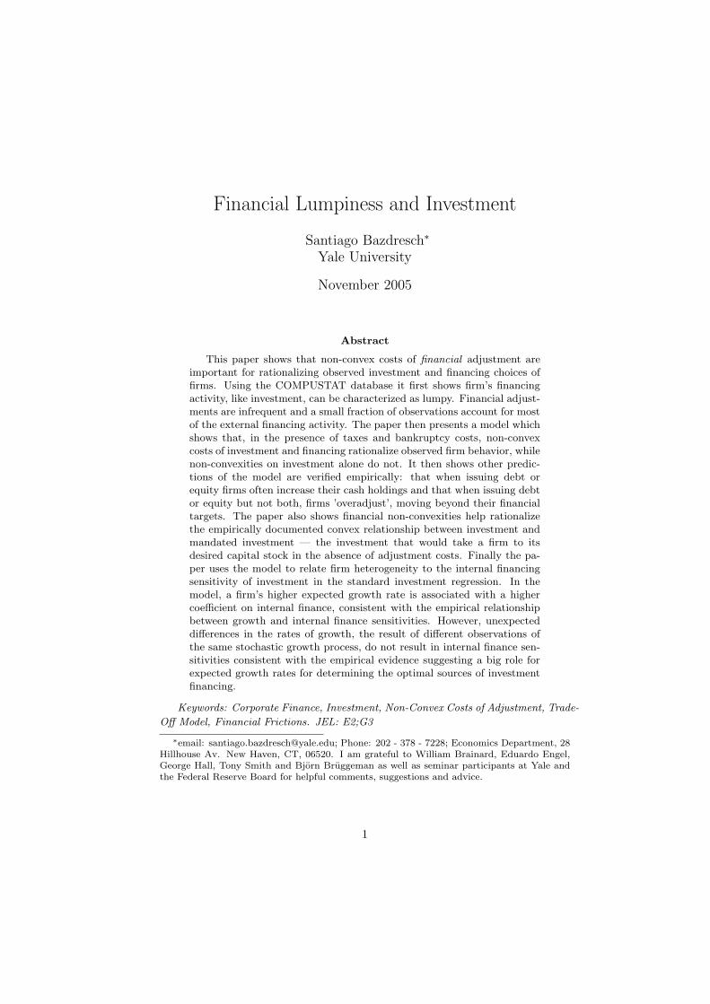
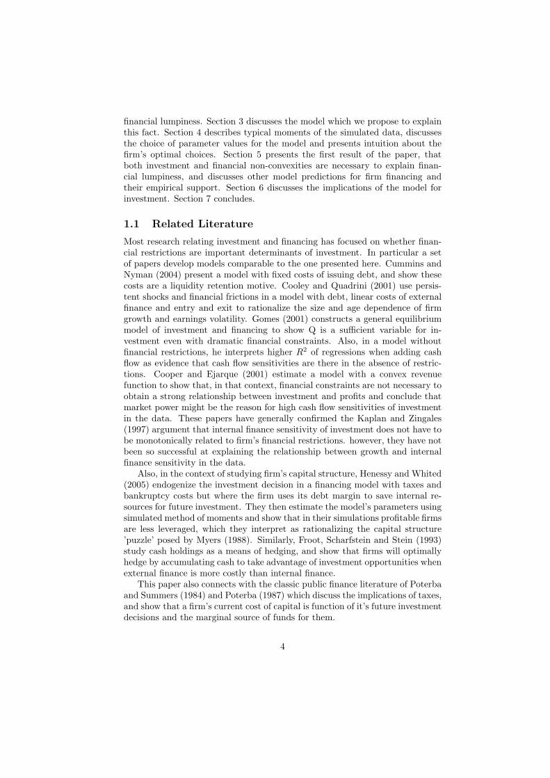
Figure 1 documents the fact that debt issuance of firms is lumpy.2 To con-struct this figure we obtain the ratio of debt issuance to assets for each firm-yearpair, for firms with continuous quarterly observations between 1984 and 2003.Within each firm we then rank these ratios from highest to lowest, and con-struct the averages over all firms by rank. The n’th bar in this figure representsthe average across firms of the n’th largest debt issuance to total assets ratio.The line in this figure represents the results of performing the same ranking andaveraging exercise for normal independent observations.3 As can be observed,in the data, a small number of periods account for most of the financial actionfor each firm, much more so than a normal distribution would imply. In 80% ofthe firm-year observations, debt issuance was less than 3% of total assets, while5% of the periods accounted for 40% of the total debt issuance observed. Thecorresponding figures for a normally distributed variable normalized to repre-sent the same gross issuance are 68% of observations below 3% of assets and 5%of observations accounting for 21% of debt issuance. The standard measure offat-tailedness, excess kurtosis, is 151 for firm’s debt issuance.
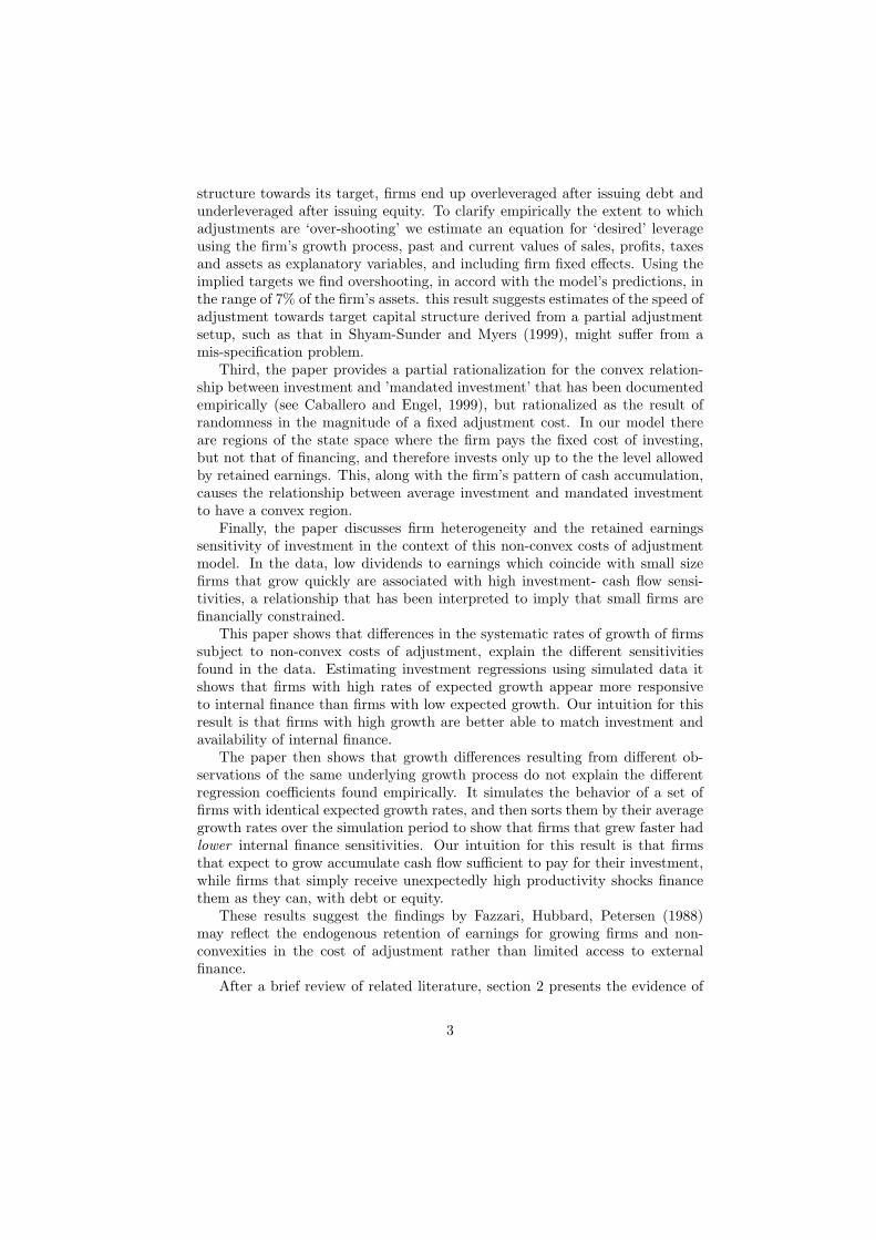
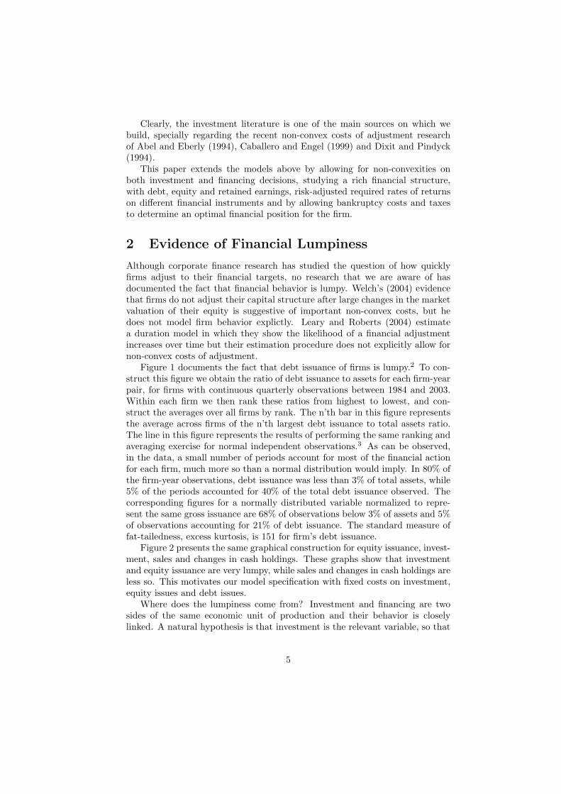
Figure 2 presents the same graphical construction for equity issuance, invest-ment, sales and changes in cash holdings. These graphs show that investmentand equity issuance are very lumpy, while sales and changes in cash holdings areless so. This motivates our model specification with fixed costs on investment,equity issues and debt issues.
Where does the lumpiness come from? Investment and financing are twosides of the same economic unit of production and their behavior is closelylinked. A natural hypothesis is that investment is the relevant variable, so that
5
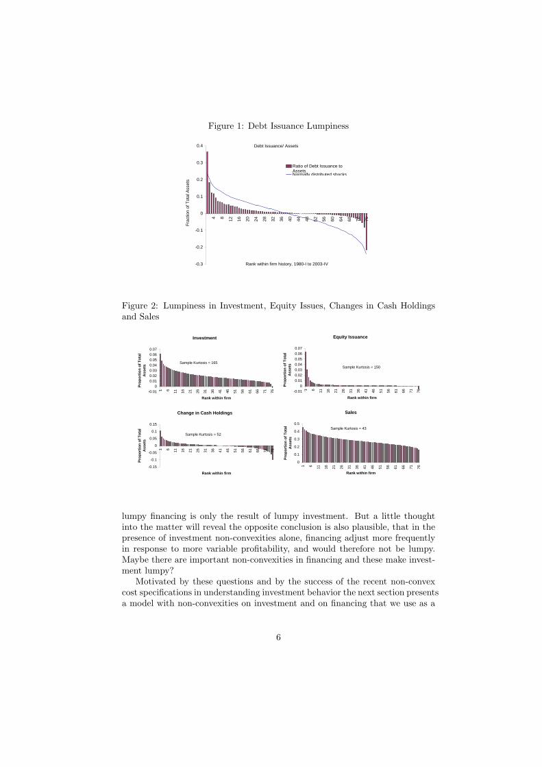
Figure 1: Debt Issuance Lumpiness
Debt Issuance/ Assets
-0.3
-0.2
-0.1
0
0.1
0.2
0.3
0.4
767268646056524844403632282420161284
Rank within firm history, 1980-I to 2003-IV
Fra
ctio
n of
Tot
al A
sset
s
Ratio of Debt Issuance toAssetsNormally distributed shocks
Figure 2: Lumpiness in Investment, Equity Issues, Changes in Cash Holdingsand Sales
year<2003 & year>1983
Freq.
Cash52
Change in Cash Holdings
-0.15
-0.1
-0.05
0
0.05
0.1
0.15
767166615651464136312621161161
Rank within firm
Pro
po
rtio
n o
f T
ota
l A
sset
s
Sample Kurtosis = 52
Sales
0
0.1
0.2
0.3
0.4
0.5767166615651464136312621161161
Rank within firm
Pro
po
rtio
n o
f T
ota
l A
sset
s
Sample Kurtosis = 43
Investment
-0.010
0.010.020.030.040.050.060.07
767166615651464136312621161161
Rank within firm
Pro
po
rtio
n o
f T
ota
l A
sset
s
Sample Kurtosis = 165
Equity Issuance
-0.010
0.010.020.030.040.050.060.07
767166615651464136312621161161
Rank within firm
Pro
po
rtio
n o
f T
ota
l A
sset
s
Sample Kurtosis = 150
lumpy financing is only the result of lumpy investment. But a little thoughtinto the matter will reveal the opposite conclusion is also plausible, that in thepresence of investment non-convexities alone, financing adjust more frequentlyin response to more variable profitability, and would therefore not be lumpy.Maybe there are important non-convexities in financing and these make invest-ment lumpy?
Motivated by these questions and by the success of the recent non-convexcost specifications in understanding investment behavior the next section presentsa model with non-convexities on investment and on financing that we use as a
6

laboratory to try out these hypothesis.
3 Investment and Financing Model
3.1 Overview
This paper presents a model of firm investment with an elaborate financialsetting that allows us to analyze the implications of non-convex costs of adjust-ment. The firm solves an infinite horizon problem, although its expected lifeis finite due to bankruptcy. It acts on behalf of its shareholders, choosing howmuch to invest in capital, how much equity to issue or dividends to pay, howmuch long term debt to issue, how much cash to accumulate and whether todeclare bankruptcy or not. Taxes, the risk of bankruptcy, and different requiredrates of return across financial instruments are modeled explicitly. Tax rateson corporate profits, dividend income and interest income imply debt financingis more ’tax efficient’ than equity financing. However, the risk of bankruptcy,which is assumed to have real costs, limits the proportion of financing that isoptimally obtained from debt. These factors are included for added realism, butalso because they imply that although funds are supplied elastically by investors,the firm is always in an interior point between all-debt and all-equity financing.Finally, cash accumulation allows the firm to retain earnings for investment ordebt repayment. Cash however is assumed to pay a liquidity premium implyingthe firm does not keep cash unless it plans to make use of it soon.
We then assume the firm cannot choose these variables freely. It pays costsof adjustment on gross investment, on debt issues or repurchases, net of matur-ing debt, and on equity issuance. It pays a fixed cost of undertaking positiveinvestment, and receives a fraction of the replacement cost of capital whendisinvesting. The costs of issuing or repurchasing debt and issuing equity areassumed to be fixed, but proportional to the scale of the firm.
3.2 Model Firm
Objective Function The firm’s objective is to obtain the highest returns forcurrent shareholders, maximizing the expected present value sum of after-taxdividends, discounted with the shareholders exogenous required rate of returnrE . The objective function of the firm is then:
max E
[Σ∞t=0
Dct
(1 + rE)t
]
where DCt denotes the current shareholder’s dividends in period t.
In addition to investment, the firm chooses debt (Bt), cash or retained earn-ings (Ct), equity issues (Xt) and dividend payments (Dt) subject to the cashflow constraint. The possibility of having contemporaneous debt and retainedearnings will allow the model to have predictions about retained earnings dis-tinct from that of a ’debt buffer’ as in Gross (1995). The firm will go bankrupt
7

if that is optimal for shareholders, in which case dividends are 0 from the timeof bankruptcy on.
In the model dividends and share repurchases are treated as equivalent,ignoring their potentially different tax implications for individual shareholders.All dividends are subject to a constant rate of taxation of τD. I assume all newequity issues are purchased by new investors and therefore constitute a ‘dilution’of original owners’ participation in the firm. In any period, the firm’s objectiveis equivalently stated as:
Vt = max(1− τD)Dt +E[Vt+1]1 + rE
(Vt
Vt + Xt
)(1)
Equation 1 expresses the value of the firm to existing shareholders as theexpected, after-tax, present discounted value of dividends allowing for the factthat equity issues will dilute the participation in future dividends. Currentstockholders only get Vt/(Vt + Xt) of the future value of the firm since theyare participating with only that proportion of the firms capital. For the firm tobe able to engage in positive equity issuance a further condition must be met,namely, that investors want to purchase this equity:
Xt ≤(
Xt
Vt + Xt
)E[Vt+1]1 + rE
(2)
The right hand side of the inequality in 2 is the value of the equity to thenew investors buying Xt of stock. The condition implies the maximum a firmcan obtain from issuing new equity issues is the actuarially fair value of the newshares.
Budget Constraint and Timing The firms budget constraint every periodis:
Dt + It + Ct+1 −BIt −Xt + (1− φ)ItId(It < 0) (3)+ Kt [ΓIId(It > 0) + ΓXId(Xt > 0) + ΓBIId(BIt 6= 0)]
= (AtKt)α − (rt + λ)Bt−1 − τC [(AtKt)α − rtBt−1 − δKt] + (1 + rF )Ct
(4)
where Id(·) represents the identifier function, rt stands for the rate of intereston debt outstanding at period t and BIt = Bt − λBt−1 stands for bond issuesnet of maturing principal.
The first two rows of equation 3 contain the firm’s decision variables, cashdeposits or retained earnings, debt issues, dividends, equity issues and grossinvestment as well as the adjustment costs associated with the firms’ decisions.The right hand side contains the predetermined variables in period t, the firm’srevenue, taxes, cash holdings and interest and principal payments to bondhold-ers.
Figure 3 details the time line of the model. Each period starts with an ob-servation of the stochastic productivity level. The firm then decides to continue
8
Figure 3: Time Line
t t+1
Firm decides to go bankrupt or not.
Productivity Atshock is observed
Firm sets investment It and financing: dividends Dt, equity issues Xt, debt
issues BIt, and cash Ct.
Firm produces (AtKt)α pays debt obligations (rt-1+λ)Bt-1
and taxes τc [(AtKt)α- rt-1Bt-1-δKt]
or to go bankrupt depending on the expected return to shareholders given thatproductivity level. If continuation is the optimal action, the firm engages inproduction, meets its debt payments, pays the corresponding taxes and makesinvestment and financing decisions that will determine the situation of the firmin the following period.
Output and Capital The source of firm income to pay dividends is thesale of output. In this model we assume, as is standard in the literature4
(i.e. Henessy and Whited, 2005), that the firm has a convex revenue func-tion R(At,Kt) = (AtKt)α. The firm’s capital evolves over time because ofinvestment (or disinvestment) and depreciation. We assume the economic rateof depreciation and the tax-related appraisal of this depreciation are equal andrepresent them with δ. 5
Investment It and depreciation then drive the evolution of capital: Kt+1 =Kt(1− δ)+ It. The firm invests and disinvests in response to changing ’produc-tivity’ level At. this productivity level is modeled as an exogenous stochasticprocess that follows a geometric random walk:
At = At−1 · ξt
ξt ∼ lognormal(µ, σ)
We define the ‘desired level of capital’ K∗t , as a function of productivity, the
cost of capital and the rate of capital depreciation, to be:
K∗t = arg max (AtKt)
α − (r + δ)Kt ⇐⇒ K∗t =
(αAα
t
r + δ
) 11−α
(5)
This desired level of capital corresponds to the optimal level of capital in aneo-classical, no cost of adjustment, single rate of discount model where At is
9

the expected value of productivity.
Cash Holdings Cash holdings (Ct) correspond to a firm’s bank deposits andare assumed to earn the risk free interest rate rf . Cash is crucial in this model. Itis a buffer stock that allows the firm to accumulate retained earnings for makinglarge, infrequent investments and avoiding frequent issues of debt or equity. Thisis a distinctive feature of our model. Others have proposed summarizing debtand cash in one variable and treating negative debt as cash (i.e. Bayer (2004)and Henessy and Whited (2005)), however that choice doesn’t permit an analysisof non-convex costs of debt issuance, nor can it account for internal financialresources explicitly in investment regressions.
Debt, bankruptcy and endogenous interest rates The crucial intuitionabout the firm’s optimal financial mix is that it is an interior point betweenall debt, all equity, and all retained earnings financing. This interior point isdetermined by taxes, the required rates of return on debt and equity, and thebankruptcy costs associated with debt. In the absence of costs of adjustment,the firm would always find it optimal to adjust to changes in current and futureexpected profitability, the main determinants of tax benefits and bankruptcycosts.
The firm issues debt with a face value of Bt and with a variable one periodinterest rate rt in period t. This rate of interest reflects the required rate ofreturn of bondholders rB the taxation of interest payments at a rate of τP
as well as the possibility that the firm will go bankrupt, defaulting on theseobligations. We set rf < rB < rE to reflect a liquidity premium on the cashholdings of the firm and a risk premium on the valuation of equity returns.Allowing for both debt and equity financing and then adjusting the valuationof debt and equity returns for their riskiness is also a non-standard feature ofthis model.
Equation 6 determines the interest rate paid by the firm on its outstandingdebt. It reflects the fact that we assume bondholders receive the scrap value ofthe firm’s capital, φKt in case of bankruptcy (Solventt = 0) and their promisedpayment if the firm is solvent (Solvent = 1).
rt =1
1− τP
(1 + rB)Bt − E[φKt ∗ (1− Solventt)]BtE[Solventt]
(6)
In the model debt is long term debt, but rather than keep track of debtissued at different times, we assume it has an exogenous rate of ’evaporation’ ormaturation of λ.6 This rate is the analogous of a depreciation rate for capital.The firm’s indebtedness then declines autonomously until the firm pursues debtissuance anew.
Although in the real world bankruptcy is a complicated legal process, in thismodel we use a simple specification for this event. The firm goes bankrupt whenits value would be negative in the absence of default. This corresponds to a sit-uation where there is nothing the firm can do — selling capital, issuing debt or
10
issuing equity, that results in a positive share value. Shareholders receive noth-ing from the point of default on, (Dt = 0, t > TBK), and bondholders receiveBP
TBK= ψKTBK
in return, with 0 < ψ < 1, which represents the liquidationvalue of assets when the firm is closed down.
Besides different required rates of return and costs of bankruptcy, the firmfaces a set of taxes that generally render debt a more ’tax efficient’ choice offinancing. The value of the firm’s revenue is affected by three taxes: as discussedabove, shareholders pay taxes on dividends at a rate τD so that only (1 − τD)of every dollar going out of the firm as payment to equity holders reaches them;debt holders also pay taxes on interest income at a rate τP , so that a bond withan interest rate of rB implies the after tax payment received by the bondholder(when the firm is solvent) is 1 + rB(1 − τP ); finally, the firm faces taxes onprofits net of depreciation and interest payments at a rate τC , so that it paysτC [(AtKt)α − δKt − rB
t Bt] in taxes to the government.This setup has important implications for firm behavior. First, it introduces
a ’wedge’ between inside and outside funds. A firm might take advantage ofan investment opportunity using retained earnings that it would not pursue ifit needed external financing for it. This also implies that the path of futureinvestment needs of a firm affect its current ‘cost of capital’. Second, note thatrevenues to bondholders are taxed once, with taxes on interest payments, whilereturns to shareholders are taxed twice, with taxes on corporate profits, andthen with taxes on dividends. Therefore, debt is more ’tax-efficient’ and thefirm will benefit from issuing debt by taking advantage of the lower tax on bondincome.
Note how an extra dollar of equity for an investment paying 1+r dollars afterdepreciation, assuming only the profits are returned to shareholders implies anet value for them of: r(1−τD)(1−τC)−rE
(1+rE). With a required rate of returns on
bonds of rB/(1− τP ), the same operation financed with debt has a net value toequity holders of (r−rB/(1−τP ))(1−τD)(1−τC)
(1+rE)that is, a 0 investment today and a
return net of interest payments tomorrow. The bond operation return is largerthan the equity operation one as long as rE(1− τP ) > rB(1− τD)(1− τC). Thisnon-neutrality of taxes which favors debt financing over equity financing is afeature of tax schedules common to many countries around the world.
Despite the three different tax rates considered, this is a gross simplificationof the tax code faced by firms. Among the important elements of the U.S.tax code for corporations which are not part of this model are the differencebetween economic depreciation rate and ‘depreciation allowances’, which let thefirm postpone its tax payments by assessing a fast rate of depreciation on itscapital; investment tax credits, which allow a firm to reduce or postpone itstax liabilities by a proportion of its investment; and loss carry back and carryforward provisions which allow the firm to ‘use’ losses from past or future periodsto reduce today’s tax liabilities.
Non-Convex Costs of Adjustment Non convexities are one of the distinc-tive features of this model and are the focus of this paper. The firm is assumed
11

to face non-convex costs of adjustment on its investment and external financing.It incurs a fixed cost of KΓIId(I > 0) when making a positive gross investment.It also faces a fixed cost KΓXId(x > 0) of issuing equity and a cost of issuingor repurchasing debt KΓBIId(BIt 6= 0).
Note that these three costs are fixed in the sense that they are independentof the size of the firm’s adjustment, and should be interpreted as the cost toproduction and to firm profitability of the adjustment process. This interpre-tation is intuitive for the cost of investment, it is easy to imagine a firm plantthat has to shut down for a ’retooling’, but they can be interpreted similarly astransaction costs and underwriting fees for equity and debt. We make the as-sumption of costs proportional to the scale of the firm for convenience in solvingthe model.
The last ’friction’ in the model is a cost of disinvestment represented by awedge between the original and the resale prices of capital. The firm can sellcapital at a fraction φ < 1 of its replacement cost. This assumption is groundedon a large body of empirical evidence documenting that firm capital is highlyindustry specific and that the scrap value and second hand values of capital aresubstantially below their depreciated value or replacement cost. 7
4 Calibration and Optimal Firm Behavior
4.1 Model Parameters
The standard parameters we use are comparable to those in the recent literature.
• α: Estimates of the degree of market power in the literature vary widely,with Hall (1988) reporting evidence of prices below marginal cost for arange of industries, Burnside (1996) reporting returns to scale being justunder 1 and Cooper and Ejarque (2001) estimating the convexity para-meter to be 0.689. A value of α closer to 1 has three main implications, alower ratio of profits to capital, a higher variance of this ratio and a higherelasticity of the firm’s desired capital level to changes in profitability. Inthe frictionless neoclassical setting, without taxes and with a fixed cost ofcapital r, the optimal capital level is K∗ = (αE[Aα]/(r + δ))(1/(1 − α))which then results in a ratio of revenues to capital of (r + δ)/α and anelasticity of desired capital to changes in E[Aα] of 1/(1−α). For the pur-pose of financial decisions of firms, a value of α closer to 1 implies the firmtends to use more external financing, first because it has less profits to useas internal financing, and second, because its desired capital level is morevolatile and it will find itself unable to finance investment out of retainedearnings more often. However, it also implies the firm has a lower averageleverage because lower profitability leads the firm to declare bankruptcyat lower relative levels of indebtedness.
• δ: Ramey and Shapiro (2001) estimate a rate of depreciation for capitalbetween 10% and 7% for their sample of aerospace firms, while Nadiri
12
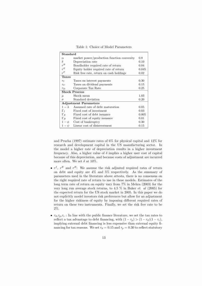
Table 1: Choice of Model Parameters
Standardα market power/production function convexity 0.8δ Depreciation rate 0.10rB Bondholder required rate of return 0.04rE Equity holder required rate of return 0.045rF Risk free rate, return on cash holdings 0.02
TaxesτI Taxes on interest payments 0.30τC Taxes on dividend payments 0.15τD Corporate Tax Rate 0.25
Shock Processµ Shock mean 1.03σ Standard deviation 0.20
Adjustment Parameters1− λ Assumed rate of debt maturation 0.05ΓI Fixed cost of investment 0.03ΓE Fixed cost of debt issuance 0.005ΓB Fixed cost of equity issuance 0.011− φ Cost of bankruptcy 0.301− ψ Linear cost of disinvestment 0.15
and Prucha (1997) estimate rates of 6% for physical capital and 12% forresearch and development capital in the US manufacturing sector. Inthe model a higher rate of depreciation results in a higher investmentfrequency. Also, a higher value of δ implies a higher user cost of capitalbecause of this depreciation, and because costs of adjustment are incurredmore often. We set δ at 10%.
• rf , rE and rB : We assume the risk adjusted required rates of returnon debt and equity are 4% and 5% respectively. As the summary ofparameters used in the literature above attests, there is no consensus onthe right required rate of return to use in these models. Estimates of thelong term rate of return on equity vary from 7% in Mehra (2003) for thevery long run average stock returns, to 4.5 % in Baker et. al (2005) forthe expected return for the US stock market in 2005. In this paper we donot explicitly model investors risk preferences but allow for an adjustmentfor the higher riskiness of equity by imposing different required rates ofreturn on these two instruments. Finally, we set the risk free rate to be2%.
• τd,τp,τc : In line with the public finance literature, we set the tax rates toreflect a tax advantage to debt financing, with (1− τp) > (1− τd)(1− τc),implying external debt financing is less expensive than external equity fi-nancing for tax reasons. We set τd = 0.15 and τp = 0.30 to reflect statutory
13
tax rates for individuals on dividends and interest income and τc = 0.20which is below the firm’s income tax rate, to reflect the widespread use ofcorporate tax shelters. In our model the average debt to capital ratio is45% comparable to the leverage ratio in the data of 33%.
• σ and µ: We set µ to reflect the average growth rate of assets of COM-PUSTAT firms from 1983 to 2002 under the assumption that α = 0.70.We set σ to imply a standard deviation of sales to capital of 15%.
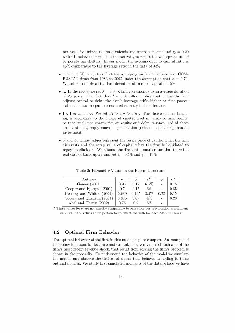
• λ: In the model we set λ = 0.95 which corresponds to an average durationof 25 years. The fact that δ and λ differ implies that unless the firmadjusts capital or debt, the firm’s leverage drifts higher as time passes.Table 2 shows the parameters used recently in the literature.
• ΓI , ΓBI and ΓX : We set ΓI > ΓX > ΓBI . The choice of firm financ-ing is secondary to the choice of capital level in terms of firm profits,so that small non-convexities on equity and debt issuance, 1/3 of thoseon investment, imply much longer inaction periods on financing than oninvestment.
• φ and ψ: These values represent the resale price of capital when the firmdisinvests and the scrap value of capital when the firm is liquidated torepay bondholders. We assume the discount is smaller and that there is areal cost of bankruptcy and set φ = 85% and ψ = 70%.
Table 2: Parameter Values in the Recent Literature
Authors α δ rE φ σ∗
Gomes (2001) 0.95 0.12 6.5% - 0.15Cooper and Ejarque (2001) 0.7 0.15 6% - 0.85Henessy and Whited (2004) 0.689 0.145 2.5% 0.75 0.15Cooley and Quadrini (2001) 0.975 0.07 4% - 0.28
Abel and Eberly (2002) 0.75 0.9 5% -* These values for σ are not directly comparable to ours since our specification is a random
walk, while the values above pertain to specifications with bounded Markov chains.
4.2 Optimal Firm Behavior
The optimal behavior of the firm in this model is quite complex. An example ofthe policy functions for leverage and capital, for given values of cash and of thefirm’s most recent revenue shock, that result from solving the firm’s problem isshown in the appendix. To understand the behavior of the model we simulatethe model, and observe the choices of a firm that behaves according to theseoptimal policies. We study first simulated moments of the data, where we have
14
attempted to replicate our empirical sample by simulating 3 thousand firms overa 20 year period. Then we analyze the time series of choices of a particular firm.
4.2.1 Simulated Moments
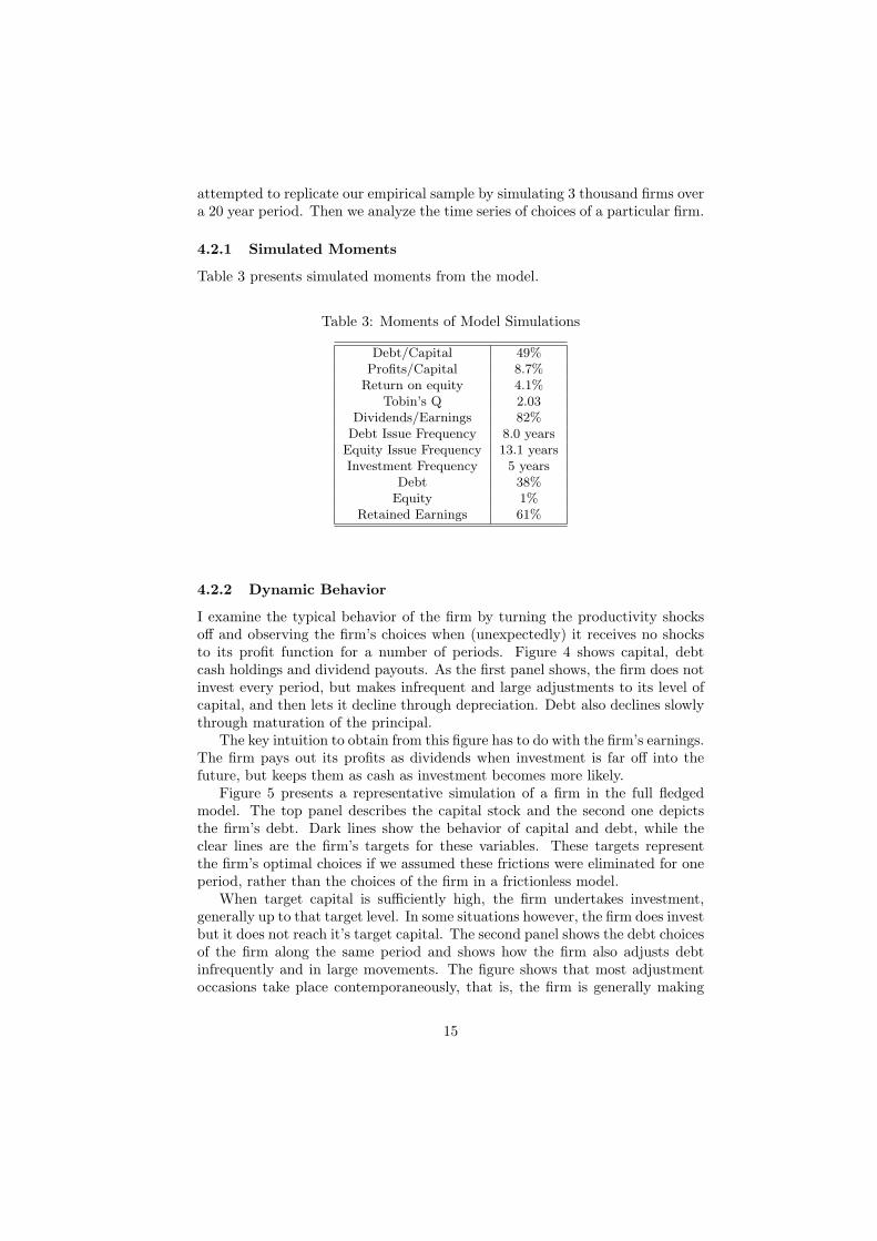
Table 3 presents simulated moments from the model.
Table 3: Moments of Model Simulations
Debt/Capital 49%Profits/Capital 8.7%
Return on equity 4.1%Tobin’s Q 2.03
Dividends/Earnings 82%Debt Issue Frequency 8.0 years
Equity Issue Frequency 13.1 yearsInvestment Frequency 5 years
Debt 38%Equity 1%
Retained Earnings 61%
4.2.2 Dynamic Behavior
I examine the typical behavior of the firm by turning the productivity shocksoff and observing the firm’s choices when (unexpectedly) it receives no shocksto its profit function for a number of periods. Figure 4 shows capital, debtcash holdings and dividend payouts. As the first panel shows, the firm does notinvest every period, but makes infrequent and large adjustments to its level ofcapital, and then lets it decline through depreciation. Debt also declines slowlythrough maturation of the principal.
The key intuition to obtain from this figure has to do with the firm’s earnings.The firm pays out its profits as dividends when investment is far off into thefuture, but keeps them as cash as investment becomes more likely.
Figure 5 presents a representative simulation of a firm in the full fledgedmodel. The top panel describes the capital stock and the second one depictsthe firm’s debt. Dark lines show the behavior of capital and debt, while theclear lines are the firm’s targets for these variables. These targets representthe firm’s optimal choices if we assumed these frictions were eliminated for oneperiod, rather than the choices of the firm in a frictionless model.
When target capital is sufficiently high, the firm undertakes investment,generally up to that target level. In some situations however, the firm does investbut it does not reach it’s target capital. The second panel shows the debt choicesof the firm along the same period and shows how the firm also adjusts debtinfrequently and in large movements. The figure shows that most adjustmentoccasions take place contemporaneously, that is, the firm is generally making
15

Figure 4: Firm Behavior Without Shocks
0 10 20 30 40 50 60 70 80 90 1000.2
0.4
0.6
0.8
1
K
Capital and Target
0 10 20 30 40 50 60 70 80 90 1000
0.1
0.2
0.3
0.4
0.5
B
Debt
0 10 20 30 40 50 60 70 80 90 1000
0.1
0.2
0.3
0.4
C
Cash
0 10 20 30 40 50 60 70 80 90 1000
0.05
0.1
D
Dividends
an investment when it issues debt and vice versa. When the firm undertakesadjustment in both variables it attains its costless adjustment targets. However,there are periods in which the firm adjusts debt or capital but not both. Inthose situations the firm does not go all the way towards its one period costlessadjustment target. The next two panels complete the picture by showing thecontemporaneous movements in cash holdings, dividend payments. Two thingsstand out from these panels. First, the firm pays high dividends just afterincreasing it’s capital stock, and second the firm saves cash in order to investor to reduce its outstanding debt.
5 Results
5.1 Financial Lumpiness
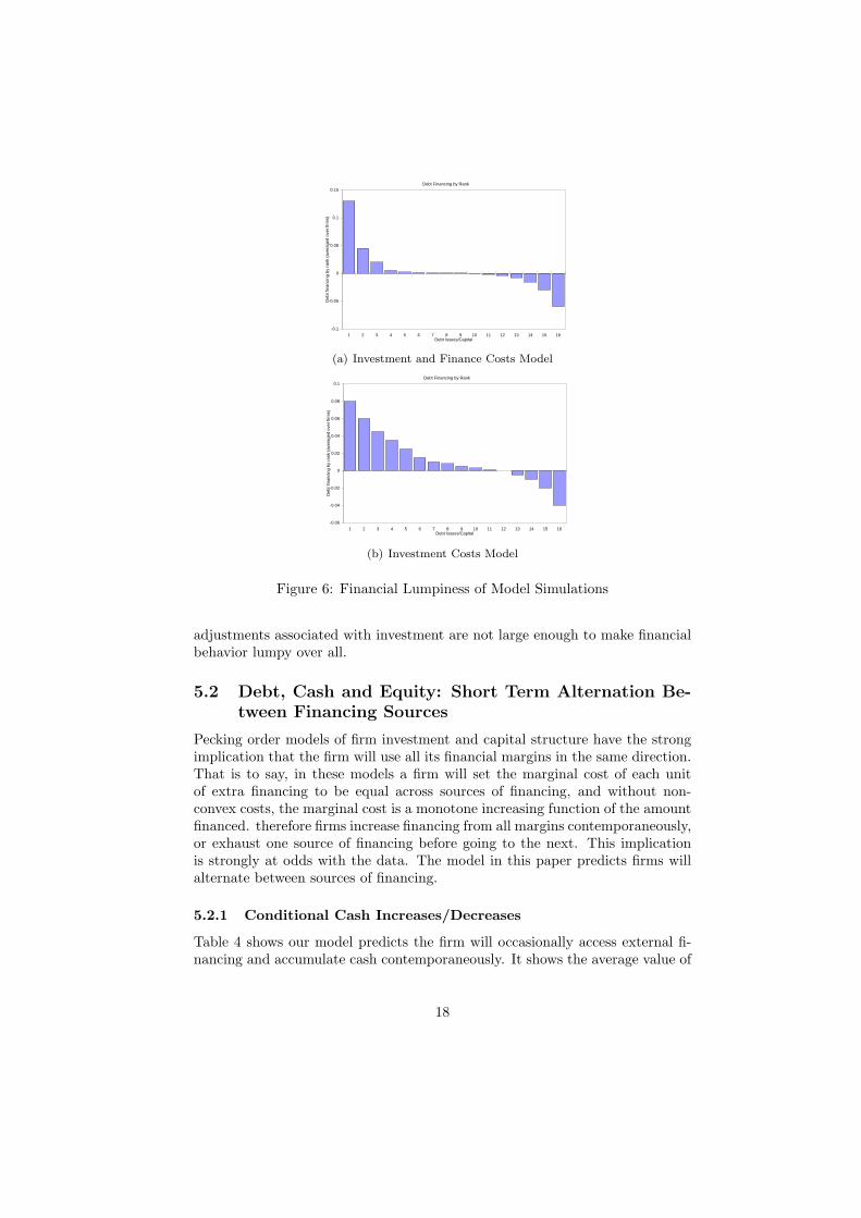
The model described above is able to rationalize the debt issuing pattern de-scribed in section 2. The two panels of figure 6 compare the issuing patternspredicted by the model with and without financial non-convex costs of adjust-ment. Each panel shows the result of simulating the behavior of 2000 firms for
16
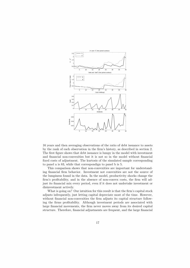
Figure 5: Model Simulation: Capital and Target Capital
5 10 15 20 25 30 35 40
0.5
1
1.5
2
2.5
( K and K* (One period costless)
K ,
K
*
K
K*
5 10 15 20 25 30 35 40
0.5
1
1.5
2
Debt and Debt* (One period costless)
Fac
e V
alue
of
Deb
t
B
B*
5 10 15 20 25 30 35 400
0.2
0.4
0.6
0.8
Cash Holdings)
Cas
h
5 10 15 20 25 30 35 40
0.02
0.04
0.06
Dividends
Div
iden
ds
16 years and then averaging observations of the ratio of debt issuance to assetsby the rank of each observation in the firm’s history, as described in section 2.The first figure shows that debt issuance is lumpy in the model with investmentand financial non-convexities but it is not so in the model without financialfixed costs of adjustment. The kurtosis of the simulated sample correspondingto panel a is 83, while that correspondign to panel b is 5.
This comparison shows that non-convexities are important for understand-ing financial firm behavior. Investment not convexities are not the source ofthe lumpiness found in the data. In the model, productivity shocks change thefirm’s profitability, and in the absence of non-convex costs, the firm will ad-just its financial mix every period, even if it does not undertake investment ordisinvestment actively.
What is going on? Our intuition for this result is that the firm’s capital stockadjusts infrequently, just letting capital depreciate most of the time. However,without financial non-convexities the firm adjusts its capital structure follow-ing the firms profitability. Although investment periods are associated withlarge financial movements, the firm never moves away from its desired capitalstructure. Therefore, financial adjustments are frequent, and the large financial
17
Debt Financing by Rank
-0.1
-0.05
0
0.05
0.1
0.15
1 2 3 4 5 6 7 8 9 10 11 12 13 14 15 16Debt Issues/Capital
Deb
t fin
anci
ng b
y ra
nk (
aver
aged
ove
r fir
ms)
(a) Investment and Finance Costs Model
Debt Financing by Rank
-0.06
-0.04
-0.02
0
0.02
0.04
0.06
0.08
0.1
1 2 3 4 5 6 7 8 9 10 11 12 13 14 15 16Debt Issues/Capital
Deb
t fin
anci
ng b
y ra
nk (
aver
aged
ove
r fir
ms)
(b) Investment Costs Model
Figure 6: Financial Lumpiness of Model Simulations
adjustments associated with investment are not large enough to make financialbehavior lumpy over all.
5.2 Debt, Cash and Equity: Short Term Alternation Be-tween Financing Sources
Pecking order models of firm investment and capital structure have the strongimplication that the firm will use all its financial margins in the same direction.That is to say, in these models a firm will set the marginal cost of each unitof extra financing to be equal across sources of financing, and without non-convex costs, the marginal cost is a monotone increasing function of the amountfinanced. therefore firms increase financing from all margins contemporaneously,or exhaust one source of financing before going to the next. This implicationis strongly at odds with the data. The model in this paper predicts firms willalternate between sources of financing.
5.2.1 Conditional Cash Increases/Decreases
Table 4 shows our model predicts the firm will occasionally access external fi-nancing and accumulate cash contemporaneously. It shows the average value of
18
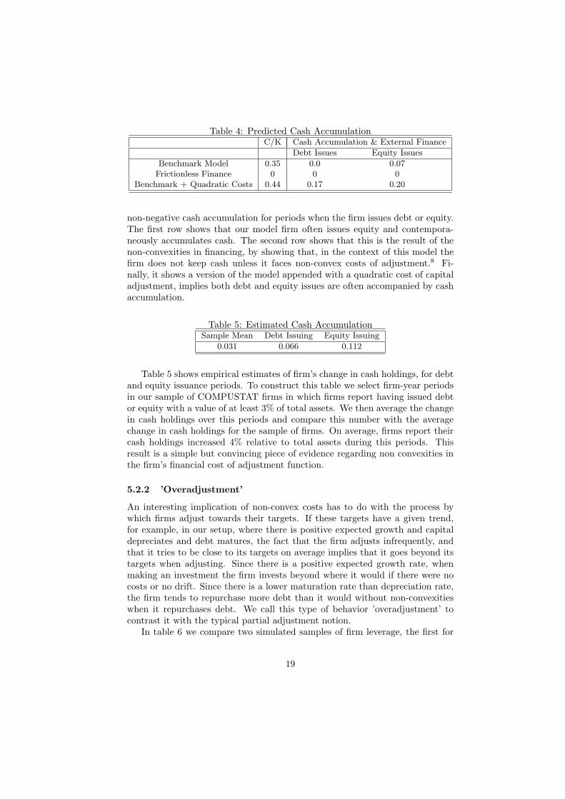
Table 4: Predicted Cash AccumulationC/K Cash Accumulation & External Finance
Debt Issues Equity Issues
Benchmark Model 0.35 0.0 0.07Frictionless Finance 0 0 0
Benchmark + Quadratic Costs 0.44 0.17 0.20
non-negative cash accumulation for periods when the firm issues debt or equity.The first row shows that our model firm often issues equity and contempora-neously accumulates cash. The second row shows that this is the result of thenon-convexities in financing, by showing that, in the context of this model thefirm does not keep cash unless it faces non-convex costs of adjustment.8 Fi-nally, it shows a version of the model appended with a quadratic cost of capitaladjustment, implies both debt and equity issues are often accompanied by cashaccumulation.
Table 5: Estimated Cash AccumulationSample Mean Debt Issuing Equity Issuing
0.031 0.066 0.112
Table 5 shows empirical estimates of firm’s change in cash holdings, for debtand equity issuance periods. To construct this table we select firm-year periodsin our sample of COMPUSTAT firms in which firms report having issued debtor equity with a value of at least 3% of total assets. We then average the changein cash holdings over this periods and compare this number with the averagechange in cash holdings for the sample of firms. On average, firms report theircash holdings increased 4% relative to total assets during this periods. Thisresult is a simple but convincing piece of evidence regarding non convexities inthe firm’s financial cost of adjustment function.
5.2.2 ’Overadjustment’
An interesting implication of non-convex costs has to do with the process bywhich firms adjust towards their targets. If these targets have a given trend,for example, in our setup, where there is positive expected growth and capitaldepreciates and debt matures, the fact that the firm adjusts infrequently, andthat it tries to be close to its targets on average implies that it goes beyond itstargets when adjusting. Since there is a positive expected growth rate, whenmaking an investment the firm invests beyond where it would if there were nocosts or no drift. Since there is a lower maturation rate than depreciation rate,the firm tends to repurchase more debt than it would without non-convexitieswhen it repurchases debt. We call this type of behavior ’overadjustment’ tocontrast it with the typical partial adjustment notion.
In table 6 we compare two simulated samples of firm leverage, the first for
19
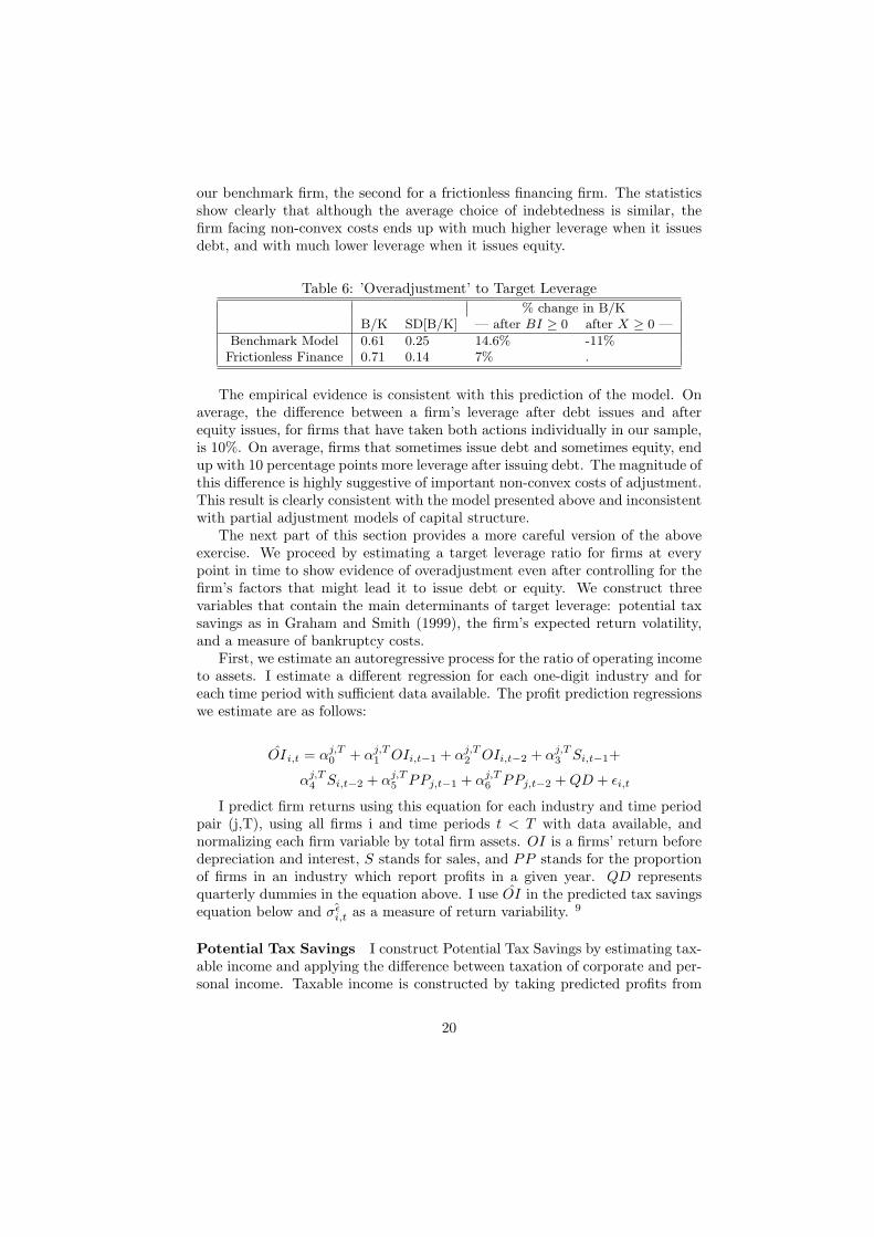
our benchmark firm, the second for a frictionless financing firm. The statisticsshow clearly that although the average choice of indebtedness is similar, thefirm facing non-convex costs ends up with much higher leverage when it issuesdebt, and with much lower leverage when it issues equity.
Table 6: ’Overadjustment’ to Target Leverage% change in B/K
B/K SD[B/K] — after BI ≥ 0 after X ≥ 0 —
Benchmark Model 0.61 0.25 14.6% -11%Frictionless Finance 0.71 0.14 7% .
The empirical evidence is consistent with this prediction of the model. Onaverage, the difference between a firm’s leverage after debt issues and afterequity issues, for firms that have taken both actions individually in our sample,is 10%. On average, firms that sometimes issue debt and sometimes equity, endup with 10 percentage points more leverage after issuing debt. The magnitude ofthis difference is highly suggestive of important non-convex costs of adjustment.This result is clearly consistent with the model presented above and inconsistentwith partial adjustment models of capital structure.
The next part of this section provides a more careful version of the aboveexercise. We proceed by estimating a target leverage ratio for firms at everypoint in time to show evidence of overadjustment even after controlling for thefirm’s factors that might lead it to issue debt or equity. We construct threevariables that contain the main determinants of target leverage: potential taxsavings as in Graham and Smith (1999), the firm’s expected return volatility,and a measure of bankruptcy costs.
First, we estimate an autoregressive process for the ratio of operating incometo assets. I estimate a different regression for each one-digit industry and foreach time period with sufficient data available. The profit prediction regressionswe estimate are as follows:
OIi,t = αj,T0 + αj,T
1 OIi,t−1 + αj,T2 OIi,t−2 + αj,T
3 Si,t−1+
αj,T4 Si,t−2 + αj,T
5 PPj,t−1 + αj,T6 PPj,t−2 + QD + εi,t
I predict firm returns using this equation for each industry and time periodpair (j,T), using all firms i and time periods t < T with data available, andnormalizing each firm variable by total firm assets. OI is a firms’ return beforedepreciation and interest, S stands for sales, and PP stands for the proportionof firms in an industry which report profits in a given year. QD representsquarterly dummies in the equation above. I use OI in the predicted tax savingsequation below and σε
i,t as a measure of return variability. 9
Potential Tax Savings I construct Potential Tax Savings by estimating tax-able income and applying the difference between taxation of corporate and per-sonal income. Taxable income is constructed by taking predicted profits from
20
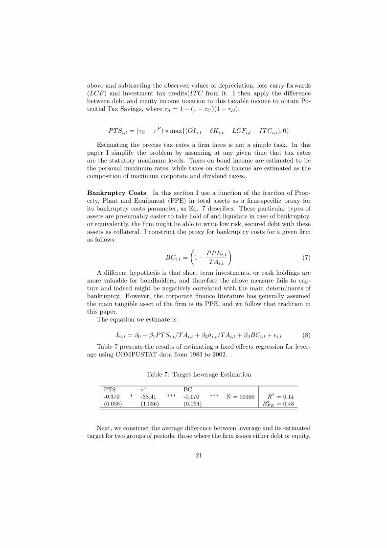
above and subtracting the observed values of depreciation, loss carry-forwards(LCF ) and investment tax credits(ITC from it. I then apply the differencebetween debt and equity income taxation to this taxable income to obtain Po-tential Tax Savings, where τS = 1− (1− τC)(1− τD).
PTSi,t = (τS − τP ) ∗max{(OIi,t − δKi,t − LCFi,t − ITCi,t), 0}
Estimating the precise tax rates a firm faces is not a simple task. In thispaper I simplify the problem by assuming at any given time that tax ratesare the statutory maximum levels. Taxes on bond income are estimated to bethe personal maximum rates, while taxes on stock income are estimated as thecomposition of maximum corporate and dividend taxes.
Bankruptcy Costs In this section I use a function of the fraction of Prop-erty, Plant and Equipment (PPE) in total assets as a firm-specific proxy forits bankruptcy costs parameter, as Eq. 7 describes. These particular types ofassets are presumably easier to take hold of and liquidate in case of bankruptcy,or equivalently, the firm might be able to write low risk, secured debt with theseassets as collateral. I construct the proxy for bankruptcy costs for a given firmas follows:
BCi,t =(
1− PPEi,t
TAi,t
)(7)
A different hypothesis is that short term investments, or cash holdings aremore valuable for bondholders, and therefore the above measure fails to cap-ture and indeed might be negatively correlated with the main determinants ofbankruptcy. However, the corporate finance literature has generally assumedthe main tangible asset of the firm is its PPE, and we follow that tradition inthis paper.
The equation we estimate is:
Li,t = β0 + β1PTSi,t/TAi,t + β2σi,t/TAi,t + β3BCi,t + εi,t (8)
Table 7 presents the results of estimating a fixed effects regression for lever-age using COMPUSTAT data from 1983 to 2002. .
Table 7: Target Leverage Estimation
PTS σε BC-0.370 * -38.41 *** -0.170 *** N = 90100 R2 = 0.14(0.038) (1.036) (0.054) R2
FE = 0.48
Next, we construct the average difference between leverage and its estimatedtarget for two groups of periods, those where the firm issues either debt or equity,
21

LDDiff and LE
Diff . We find LEDiff is -0.07 and LD
Diff 0.03, consistent with themodel prediction of over adjustment.
Table 8: Distance from Estimated Target Leverage
Debt Issues Equity Issues
Before After (LBDiff ) Before After (LE
Diff )-0.02 0.03 -0.03 -0.07
6 Investment with Non-Convex Costs of Financ-ing
6.1 Investment Hazard Function
Despite the success of non-convex cost specifications for modeling firm invest-ment, empirical estimations of firm’s rate of investment as a function of thedistance from their mandated or target capital are not exactly consistent withnon-convex costs of adjustment. Caballero and Engel (1999) (CE), for examplefind a region where average investment is positive, but is only a proportion ofmandated investment, while fixed costs imply the firm adjusts all the way or itdoes not adjust at all. In their paper, CE rationalize this fact with fixed cost ofrandom magnitude ωt. With this stochastic costs, firms don’t have a particularpoint at which they adjust, rather, their decision depends on both mandated in-vestment and the observed fixed cost. They then argue that averaging smoothsover these random observations to create a ’partial adjustment’ region whenestimating the relationship between mandated and actual investment.
The model in this paper provides a partial rationalization for the behaviorof investment which does not rely on random fixed costs. In the model the firmoccasionally finds itself willing to pay the investment cost and not willing to paythe financing fixed cost, so that investment is undertaken but it does not coverall of mandated investment. Figure 7 presents the optimal investment policy ofa firm. It consists of cross sections of the investment policy function for differentlevels of debt assuming the firm holds cash worth 4% of the firm’s capital. Thefigure shows that there is a region of the state space where the firm pays theinvestment fixed cost but not the financing fixed costs, and therefore it investsonly from current internal resources. Then another region where it issues debt,up to a limit and finally a point after which investment grows linearly withmandated investment.
Figure 8 presents the average investment behavior of the firm as a functionof the difference between current and target capital. Although for any givenlevel of debt and cash, the investment function is a step function of mandatedinvestment like those in figure 7, the average level of investment seems to reflect
22
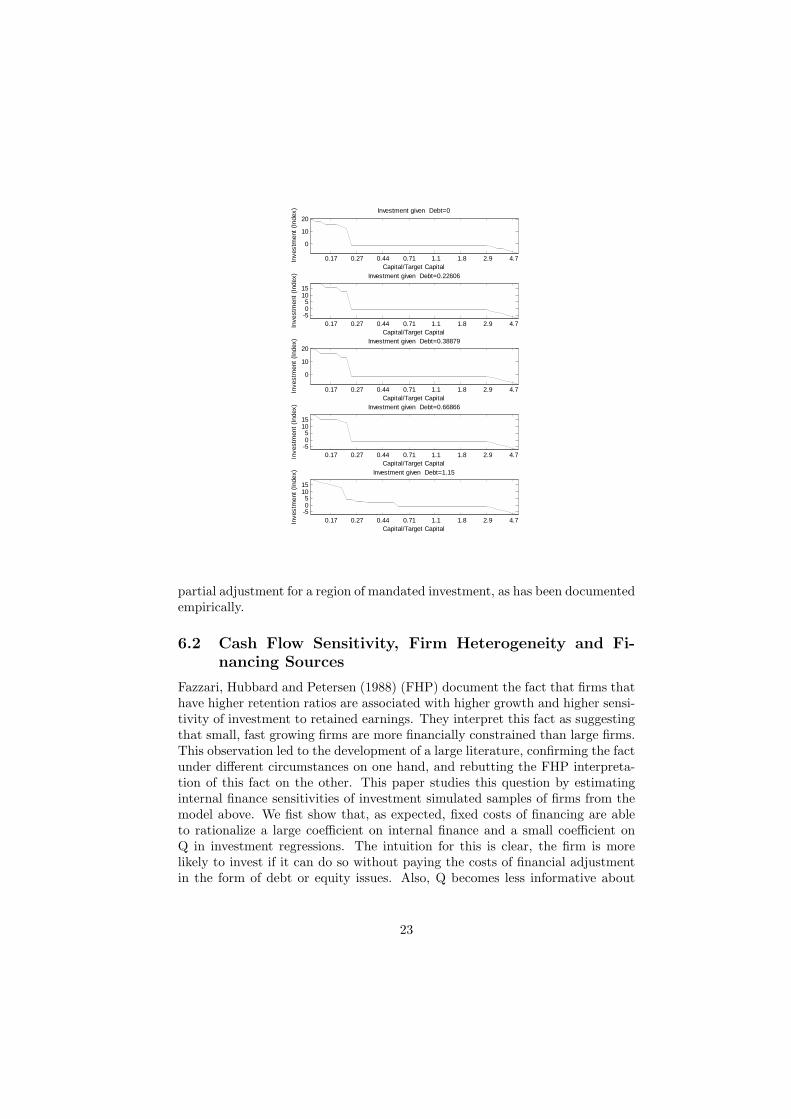
Figure 7: Investment to Mandated Investment Policies
0.17 0.27 0.44 0.71 1.1 1.8 2.9 4.7
0
10
20
Capital/Target Capital
Inve
stm
ent
(Ind
ex) Investment given Debt=0
0.17 0.27 0.44 0.71 1.1 1.8 2.9 4.7-505
1015
Capital/Target Capital
Inve
stm
ent
(Ind
ex) Investment given Debt=0.22606
0.17 0.27 0.44 0.71 1.1 1.8 2.9 4.7
0
10
20
Capital/Target Capital
Inve
stm
ent
(Ind
ex) Investment given Debt=0.38879
0.17 0.27 0.44 0.71 1.1 1.8 2.9 4.7-505
1015
Capital/Target Capital
Inve
stm
ent
(Ind
ex) Investment given Debt=0.66866
0.17 0.27 0.44 0.71 1.1 1.8 2.9 4.7-505
1015
Inve
stm
ent
(Ind
ex)
Capital/Target Capital
Investment given Debt=1.15
partial adjustment for a region of mandated investment, as has been documentedempirically.
6.2 Cash Flow Sensitivity, Firm Heterogeneity and Fi-nancing Sources
Fazzari, Hubbard and Petersen (1988) (FHP) document the fact that firms thathave higher retention ratios are associated with higher growth and higher sensi-tivity of investment to retained earnings. They interpret this fact as suggestingthat small, fast growing firms are more financially constrained than large firms.This observation led to the development of a large literature, confirming the factunder different circumstances on one hand, and rebutting the FHP interpreta-tion of this fact on the other. This paper studies this question by estimatinginternal finance sensitivities of investment simulated samples of firms from themodel above. We fist show that, as expected, fixed costs of financing are ableto rationalize a large coefficient on internal finance and a small coefficient onQ in investment regressions. The intuition for this is clear, the firm is morelikely to invest if it can do so without paying the costs of financial adjustmentin the form of debt or equity issues. Also, Q becomes less informative about
23
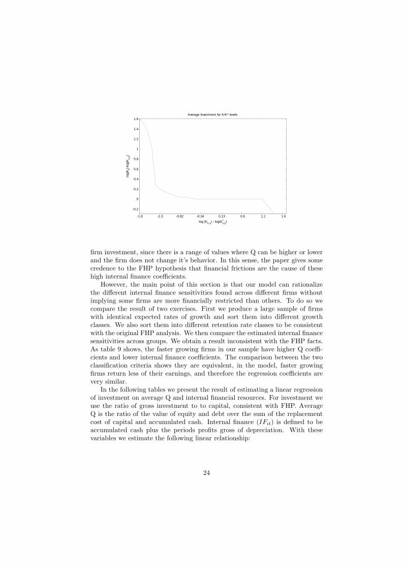
Figure 8: Average Investment to Mandated Investment
-1.8 -1.3 -0.82 -0.34 0.13 0.6 1.1 1.6
-0.2
0
0.2
0.4
0.6
0.8
1
1.2
1.4
1.6Average Investment for K/K* levels
log (Kt-1) - log(K*t-1)
log(
Kt)-
log(
Kt-
1)
firm investment, since there is a range of values where Q can be higher or lowerand the firm does not change it’s behavior. In this sense, the paper gives somecredence to the FHP hypothesis that financial frictions are the cause of thesehigh internal finance coefficients.
However, the main point of this section is that our model can rationalizethe different internal finance sensitivities found across different firms withoutimplying some firms are more financially restricted than others. To do so wecompare the result of two exercises. First we produce a large sample of firmswith identical expected rates of growth and sort them into different growthclasses. We also sort them into different retention rate classes to be consistentwith the original FHP analysis. We then compare the estimated internal financesensitivities across groups. We obtain a result inconsistent with the FHP facts.As table 9 shows, the faster growing firms in our sample have higher Q coeffi-cients and lower internal finance coefficients. The comparison between the twoclassification criteria shows they are equivalent, in the model, faster growingfirms return less of their earnings, and therefore the regression coefficients arevery similar.
In the following tables we present the result of estimating a linear regressionof investment on average Q and internal financial resources. For investment weuse the ratio of gross investment to to capital, consistent with FHP. AverageQ is the ratio of the value of equity and debt over the sum of the replacementcost of capital and accumulated cash. Internal finance (IFit) is defined to beaccumulated cash plus the periods profits gross of depreciation. With thesevariables we estimate the following linear relationship:
24
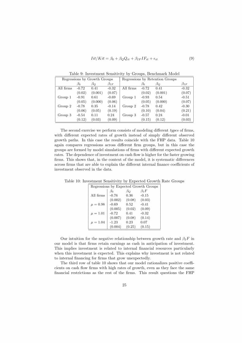
Iit/Kit = β0 + βQQit + βIF IFit + εit (9)
Table 9: Investment Sensitivity by Groups, Benchmark ModelRegressions by Growth Groups Regressions by Retention Groups
β0 βQ βIF β0 βQ βIF
All firms -0.72 0.41 -0.32 All firms -0.72 0.41 -0.32(0.02) (0.001) (0.07) (0.02) (0.001) (0.07)
Group 1 -0.91 0.61 -0.69 Group 1 -0.93 0.54 -0.51(0.05) (0.000) (0.06) (0.05) (0.000) (0.07)
Group 2 -0.78 0.35 -0.14 Group 2 -0.78 0.42 -0.30(0.06) (0.05) (0.19) (0.10) (0.04) (0.21)
Group 3 -0.54 0.11 0.24 Group 3 -0.57 0.24 -0.01(0.12) (0.03) (0.09) (0.15) (0.12) (0.03)
The second exercise we perform consists of modeling different types of firms,with different expected rates of growth instead of simply different observedgrowth paths. In this case the results coincide with the FHP data. Table 10again compares regressions across different firm groups, but in this case thegroups are formed by model simulations of firms with different expected growthrates. The dependence of investment on cash flow is higher for the faster growingfirms. This shows that, in the context of the model, it is systematic differencesacross firms that are able to explain the different internal finance coefficients ofinvestment observed in the data.
Table 10: Investment Sensitivity by Expected Growth Rate GroupsRegressions by Expected Growth Groups
β0 βQ βIFAll firms -0.76 0.36 -0.15
(0.002) (0.08) (0.03)µ = 0.98 -0.69 0.52 -0.41
(0.005) (0.02) (0.09)µ = 1.01 -0.72 0.41 -0.32
(0.007) (0.08) (0.14)µ = 1.04 -1.23 0.23 0.07
(0.004) (0.25) (0.15)
Our intuition for the negative relationship between growth rate and βIF inour model is that firms retain earnings as cash in anticipation of investment.This implies investment is related to internal financial resources particularlywhen this investment is expected. This explains why investment is not relatedto internal financing for firms that grow unexpectedly.
The third row of table 10 shows that our model rationalizes positive coeffi-cients on cash flow firms with high rates of growth, even as they face the samefinancial restrictions as the rest of the firms. This result questions the FHP
25
interpretation of the magnitude of internal finance coefficients in investmentregressions as a measure of the degree of financial restrictions facing a firm.
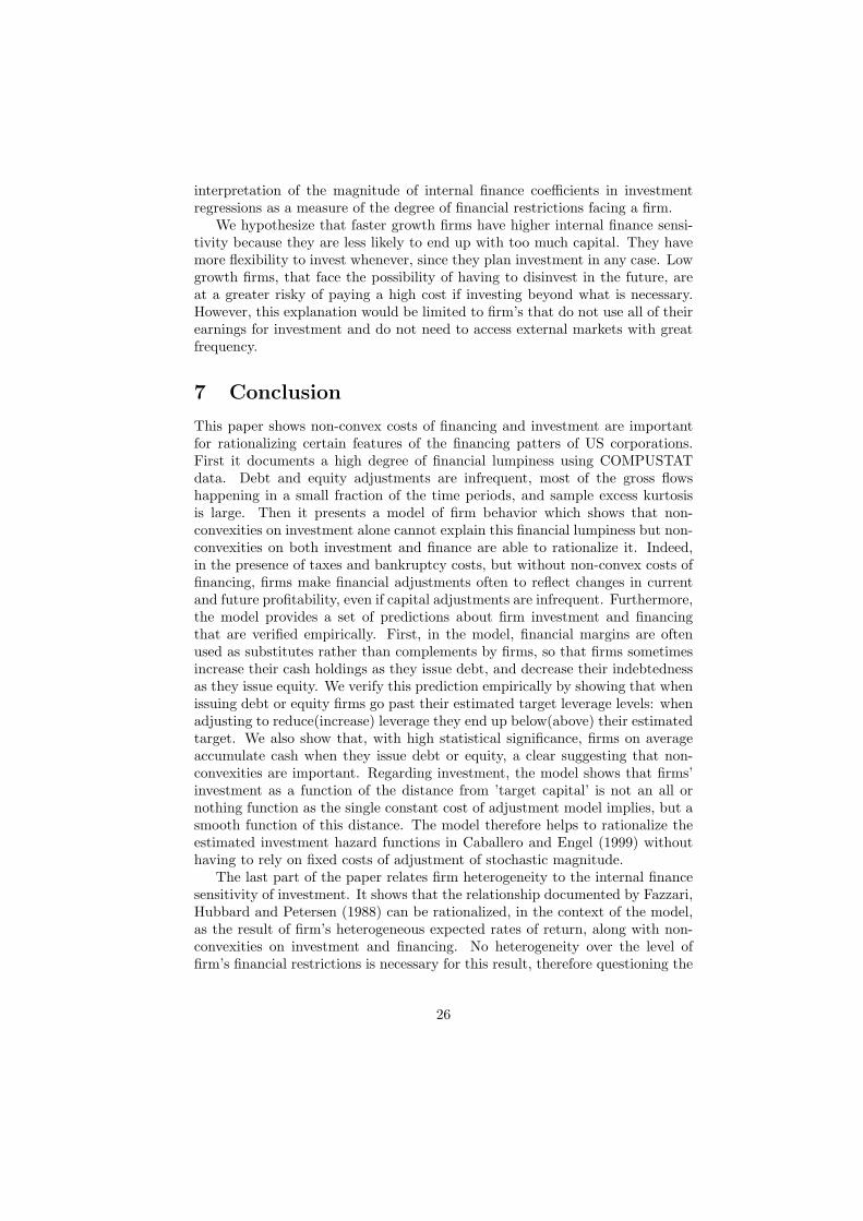
We hypothesize that faster growth firms have higher internal finance sensi-tivity because they are less likely to end up with too much capital. They havemore flexibility to invest whenever, since they plan investment in any case. Lowgrowth firms, that face the possibility of having to disinvest in the future, areat a greater risky of paying a high cost if investing beyond what is necessary.However, this explanation would be limited to firm’s that do not use all of theirearnings for investment and do not need to access external markets with greatfrequency.
7 Conclusion
This paper shows non-convex costs of financing and investment are importantfor rationalizing certain features of the financing patters of US corporations.First it documents a high degree of financial lumpiness using COMPUSTATdata. Debt and equity adjustments are infrequent, most of the gross flowshappening in a small fraction of the time periods, and sample excess kurtosisis large. Then it presents a model of firm behavior which shows that non-convexities on investment alone cannot explain this financial lumpiness but non-convexities on both investment and finance are able to rationalize it. Indeed,in the presence of taxes and bankruptcy costs, but without non-convex costs offinancing, firms make financial adjustments often to reflect changes in currentand future profitability, even if capital adjustments are infrequent. Furthermore,the model provides a set of predictions about firm investment and financingthat are verified empirically. First, in the model, financial margins are oftenused as substitutes rather than complements by firms, so that firms sometimesincrease their cash holdings as they issue debt, and decrease their indebtednessas they issue equity. We verify this prediction empirically by showing that whenissuing debt or equity firms go past their estimated target leverage levels: whenadjusting to reduce(increase) leverage they end up below(above) their estimatedtarget. We also show that, with high statistical significance, firms on averageaccumulate cash when they issue debt or equity, a clear suggesting that non-convexities are important. Regarding investment, the model shows that firms’investment as a function of the distance from ’target capital’ is not an all ornothing function as the single constant cost of adjustment model implies, but asmooth function of this distance. The model therefore helps to rationalize theestimated investment hazard functions in Caballero and Engel (1999) withouthaving to rely on fixed costs of adjustment of stochastic magnitude.
The last part of the paper relates firm heterogeneity to the internal financesensitivity of investment. It shows that the relationship documented by Fazzari,Hubbard and Petersen (1988) can be rationalized, in the context of the model,as the result of firm’s heterogeneous expected rates of return, along with non-convexities on investment and financing. No heterogeneity over the level offirm’s financial restrictions is necessary for this result, therefore questioning the
26

validity of interpreting internal finance sensitivities of investment as measuresof financial restrictions. Finally the paper shows heterogeneity in firm growththat is unexpected, the result of different growth paths for firms with the sameexpected growth rates, does not result in estimated internal finance sensitivitieslike those found empirically, suggesting heterogeneity in firms expected rates ofgrowth is important for understanding firm’s investment financing decisions.
27

Appendix
A ’Distance from target’variables
This section shows how the model above can be expressed in more condensedform, taking advantage of the homogeneity properties of the assumed functionalforms. In that way the problem’s state space is reduced from 5 to 4 dimensionsand can then be solved numerically with a reasonably fine grid. The problem isrewritten in variables and a value functions as a proportion of ‘target capital’.The key variable is now z = K/K∗and the value function V is expressed as vK∗.
First, define the target capital level K∗as the solution to the frictionlessproblem with discount rate ρ:
K∗ = arg max(AK)α − δK − rK
=(
αAα
δ + ρ
) 11−α
Then express the productivity coefficient in terms of target capital and elim-inate actual capital from the production function:
Aα = (K∗)1−α
(ρ + δ
α
)
(AK)α = (K∗)1−α
(ρ + δ
α
)Kα = K∗
(ρ + δ
α
)zα
Equation 3 can then be expressed using the ratio variables z, z, i and e:
it + dt − xt − bit − ct
− zt
{ΓIId{it>0} + ΓXId{xt>0} + ΓBIId{bit>0}
}− (1− φ)itId(it < 0)
= szαt − τC
{szα
t − δzt − rt−1bt−1
}− λbt−1 + (1 + rF )ct−1
where s =(
ρ+δα
), i = I/K∗, d = D/K∗, x = X/K∗, b = B/K∗ ct−1 =
K∗t−1/K∗
t ct−1 and bt−1 = K∗t−1/K∗
t bt−1.Therefore the Bellman equation for the problem can be written as follows:
V
K∗ = v = max
{max
i,L′,C′
[(1− τD)div − x +
(ξ′)1
1−α
1 + ρE[v′(z′, L′, C ′)]
vt
vt + xt
], 0
}
Where the forward variables z′ is constructed as follows:
z′ = (z + i) ∗K∗/(K∗′) =z + i
ξ′(1
1−α )
28

B Model Solution
This section describes the numerical procedure to find a solution to the problemabove. This solution consists of a value function V , a set of optimal policies H, and a set of interest rates r, consistent with each other:
1. V is the value of the firm derived from H and r,
2. Interest rates reflect risk neutral pricing given V and H and,
3. H is the optimal firm policy given V and r and
I solve for an approximate solution to the firm’s problem above computa-tionally. To set up the problem I construct a grid G of in the state space of the’distance from targets’ problem: GS = {St = (zt, bt, ct, ξt)|zt ∈ {z1...znz}, bt ∈{b1...bnb
}, ct ∈ {c1...cnc}, ξt ∈ {ξ1...ξnξ
}}; and one in the control space: GC ={Ct = (zt, bt, ct)|(zt, bt, ct, ξt) ∈ St}. Then I define an initial interest rate r0 :Ct− > <+ and an external equity flow function E(St, Ct|ri) : GS ×GC− > <,which denotes current income as a function of state and choice variables, givenan bond pricing schedule r.
The Bellman equation is then:
V (St) = max{
maxCt∈GC
E(St, Ct) + βE[ξ′V (S′t)], 0}
(10)
where S′t = (Ct, ξ′), V coincides with the definition above, and the expecta-
tion is over the productivity shock ξ′:
E[ξ′ ˆV (S′t)] =∑
ξ′∈ξ1...ξnξ
ξ ˆV ((Ct, ξ))r(ξ = ξ′)
Equation 10 defines a functional V(V, ri) which produces a limit value func-tion V ∗(ri), the fixed point of the functional given ri, that is V(V ∗(ri), ri) =V ∗(ri). The model however, has bond prices being a function of the firm’sexpected value, and therefore, once I obtain V ∗(ri), I construct ri+1(V ∗(ri))following equation 6.
29
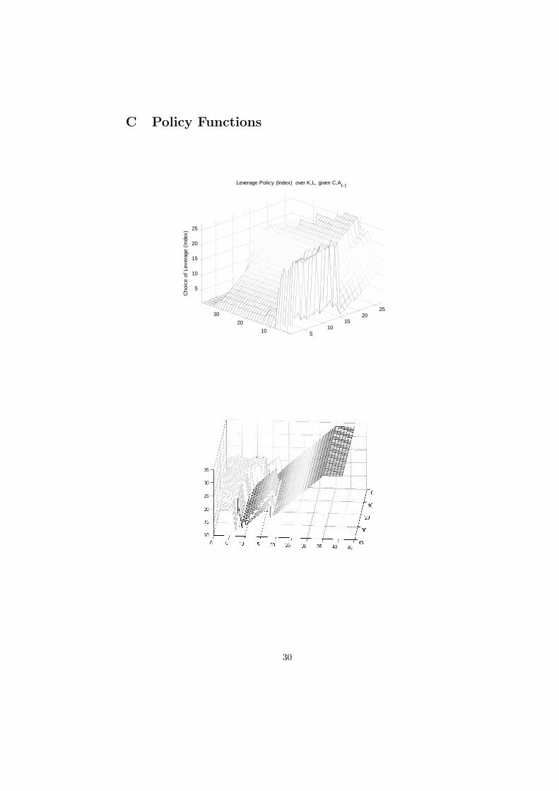
C Policy Functions
Figure 9: Leverage Policy
510
1520
25
10
20
30
5
10
15
20
25
Original Leverage (Index)
Leverage Policy (Index) over K,L, given C,At-1
Original Capital (Index)
Cho
ice
of L
ever
age
(Ind
ex)
Figure 10: Capital Policy
30

References
[1] Abel, Andrew and Janice Eberly,(2004). “Q Theory Without AdjustmentCosts & Cash Flow Effects Without Financing Constraints,” Papers of the2004 Meetings of the Society for Economic Dynamics, No. 205.
[2] Auerbach, Alan J., (2002). “Taxation and Corporate Financial Policy”, inAlan J. Auerbach and Martin Feldstein (eds.) Handbook of Public Eco-nomics Volume III, 1251-1292.
[3] Caballero, Ricardo J., (1997). “Aggregate investment: A 90s view,”, Chap-ter 12 in Handbook of Macroeconomics, John Taylor and Michael Wood-ford, Eds., North Holland, Amsterdam.
[4] Caballero Ricardo J. and Eduardo Engel, (1993). “Microeconomics adjust-ment hazards and aggregate dynamics,” Quarterly Journal of Economics108, 359-384.
[5] Caballero, Ricardo J. and Eduardo Engel, (1999). “Explaining InvestmentDynamics in U.S. Manufacturing: A Generalized (S,s) Approach,” Econo-metrica 67, No. 4, 783-826.
[6] Caballero, Ricardo J. and Leahy, John V., “Fixed Costs: The Demise ofMarginal q”, NBER Working Paper No. W5508 x
[7] Cooley, Thomas.F. and Vincenzo Quadrini, (2001). Financial markets andfirm dynamics. American Economic Review 91(5), 12861310.
[8] Cooper, Rusell and Joao Ejarque, (2001)“Exhuming Q: Market Powervs.Capital Market Imperfections,” NBER Working Paper No. W8182.
[9] Cummins, Jason and Ingmar Nyman, (2004). “Optimal Investment withFixed Financing Costs,” Finance and Economics Discussion Series No.2001-40, Federal Reserve Board.
[10] Dixit, Avinash K. and Robert S. Pindyck, (1994).Investment under Uncertainty, Princeton University Press, Princeton,N.J.
[11] Dons, Mark and Timothy Dunne, (1994). “Capital Adjustment Patterns inManufacturing,” Review of Economic Dynamics 1, 409-429.
[12] Fazzari, Steven M., R. Glenn Hubbard and Brunce C. Petersen, (1988).“Financing Constraints and Corporate Investment,” Brookings Papers onEconomic Activity 1, 14195.
[13] Froot, Kenneth A., David S. Scharfstein and Jeremy C. Stein, (1993). “RiskManagement: Coordinating Corporate Investment and Financing Policies,”The Journal of Finance 48, No. 5.
31
[14] Gomes, Joao, (2001). “Financing Investment,” American Economic Review91, No. 5, 1263-1285.
[15] Gross, David, (1995). “The Investment and Financial Decisions of LiquidityConstrained Firms” Chapters 1-3, Doctoral Dissertation, MIT.
[16] Hennessy, Christopher and Tony Whited, (2005) ”Debt Dynamics”, TheJournal of Finance 60, No. 3.
[17] Graham, John R., Clifford W. Smith Jr., (1999). “Tax Incentives to Hedge,”Journal of Finance 54, 2241-2262.
[18] Jorgenson, Dale W. (1996)“Empirical Studies of Depreciation,” EconomicInquiry 34, Vol. 1, 24-42.
[19] Nadiri, M. Ishaq and Ingmar R. Prucha ,(1997). “Estimation of the Depre-ciation Rate of Physical and R&D Capital in the U.S. Total ManufacturingSector,” NBER Working Paper No. W4591.
[20] Kwan, Simon, Willard Carleton, (1998). “Financial Contracting and theChoice Between Private Placement and Publicly Offered Bonds,” FederalReserve Bank of San Francisco working paper.
[21] Myers, Stewart C., (1984). “The Capital Structure Puzzle,” Journal ofFinance 39, 575-592.
[22] Ramey, Valerie and Matthew D. Shapiro (2001)“Displaced Capital: AStudy of Aerospace Closings,” Journal of Political Economy 10, 958-992.
[23] Roberts, Michael and Mark T. Leary (2004) “Do Firms Rebalance theirCapital Structures?”, 14th Annual Utah Winter Finance Conference Vol-ume.
[24] Shyam-Sunder, Lakshmi Stweart C. Myers, (1999). “Testing Static Trade-Off Against Pecking Order Models of Capital Structure,” Journal of Finan-cial Economics 51, 219-244.
[25] Welch, Ivo, (2004). “Capital Structure and Stock Returns,” Journal ofPolitical Economy 112, 106-31.
32
Notes
1Caballero and Engel (1999) show the changing elasticity of aggregate invest-ment to underlying fundamentals can be traced to the changing distribution offirm’s distances from desired capital stock, in a model with stochastic fixedcosts of adjustment. Caballero and Leahy (1996) show traditional investmentequations break down in the presence of non-convex costs.
2This graph is the financing analogous of figure 1 in Doms and Dunne (1998)which is constructed from manufacturing investment data.
3The normal distribution is a good benchmark. In a model with normalshocks to productivity and no costs of adjustment or other frictions, capitaland debt would both always be proportional to each other and to productivitymaking them normally distributed as well.
4We can think of this specification reflecting a firm that uses capital Kt
, labor Nt and technology At to produce Yt = f(At, Kt, Nt) units of outputand then sells each unit at a price of P (Yt). Assuming a constant returnsto scale Cobb-Douglas production function f(At,Kt, Nt) = AtK
βt N1−β
t andletting the firm adjust labor freely, output can be written in terms of capital asf(At,Kt) = KtAt,where
At = A1−β
β
t
(β − 1Wt
) 1−ββ
and Wt is the wage rate. Finally, assuming the firm faces an isoelastic de-mand function with price elasticity of −η we obtain a convex revenue functionR(At,Kt, Nt) = Yt · P (Yt) = (AtKt)α, with α = (η − 1)/η.
5Although other economists have explored capital depreciation issues by al-lowing for different depreciation rates for different capital vintages or by dis-tinguishing between depreciation and capital obsolescence, these issues are notpart of the present model. A discussion of depreciation in the context of the USincome and product accounts appears in Jorgenson (1996)
6This novel feature of our model is consistent with the fact that long termdebt issues often impose recovery fund requirements that imply the firm mustallocate funds for principal repayment. Kwan and Carrelton (2004) documentthat this is particularly the case for private issues.
7Ramey and Shapiro (2001) document high capital specificity and discountsof between 40% and 85% on the sale of displaced capital for the aerospaceindustry.
8This is a generic feature of our model. As Cummins and Nyman (1999)show, introducing a cost of external financing is in principle sufficient to make
33

the firm hedge by retaining earnings in the form of cash. In our model withoutnon-convex costs there is no extra cost of external financing.
9Details of regression estimates for a group of firms are presented in AppendixB
34