Financial intermediaries, credit Shocks and business cycles · Munich Personal RePEc Archive Financial intermediaries, credit Shocks and business cycles Mimir, Yasin University of

Munich Personal RePEc Archive

Financial intermediaries, credit Shocks

and business cycles

Mimir, Yasin

University of Maryland, College Park, Department of Economics

May 2012

Online at https://mpra.ub.uni-muenchen.de/39648/

MPRA Paper No. 39648, posted 25 Jun 2012 18:49 UTC

Financial Intermediaries, Credit Shocks and

Business Cycles∗

Yasin MimirUniversity of Maryland

May 2012

Abstract

This paper conducts a quantitative analysis of the role of financial shocks and creditfrictions affecting the banking sector in driving U.S. business cycles. I first document threekey business cycle stylized facts of aggregate financial variables in the U.S. banking sector:(i) Bank credit, deposits and loan spread are less volatile than output, while net worthand leverage ratio are more volatile, (ii) bank credit and net worth are procyclical, whiledeposits, leverage ratio and loan spread are countercyclical, and (iii) financial variables leadthe output fluctuations by one to three quarters. I then present an equilibrium businesscycle model with a financial sector, featuring a moral hazard problem between banks and itsdepositors, which leads to endogenous capital constraints for banks in obtaining funds fromhouseholds. The model incorporates empirically-disciplined shocks to bank net worth (i.e.“financial shocks”) that alter the ability of banks to borrow and to extend credit to non-financial businesses. I show that the benchmark model is able to deliver most of the abovestylized facts. Financial shocks and credit frictions in banking sector are important notonly for explaining the dynamics of financial variables but also for the dynamics of standardmacroeconomic variables. Financial shocks play a major role in driving real fluctuations dueto their impact on the tightness of bank capital constraint and the credit spread.

Keywords: Banks, Financial Fluctuations, Credit Frictions, Bank Equity, Real Fluctuations

JEL Classification: E10, E20, E32, E44

∗I thank seminar participants at the Board of Governors of the Federal Reserve System, Bank of Canada,Bank of England, Uppsala University, New Economic School, Koc University, Ozyegin University, TOBB-ETU,METU-NCC, 2011 Annual Meeting of the Society for Economic Dynamics, 2011 International Conference onComputing in Economics and Finance, 2011 Eastern Economic Association Conference, University of Maryland,2010 Midwest Macroeconomics Meetings, Bilkent University, Central Bank of the Republic of Turkey, 2010International Conference of Middle East Economic Association, 2010 International Conference on EconomicModeling for helpful comments. I am also grateful to the Federal Reserve Board for their hospitality. I alsowould like to thank S. Boragan Aruoba, Sanjay K. Chugh, Pablo N. D’Erasmo, Anton Korinek, Enrique G.Mendoza, John Shea, and Enes Sunel for very constructive suggestions. All remaining errors are mine. ContactDetails: Department of Economics, University of Maryland, 3105 Tydings Hall, College Park MD 20742. E-mail:[email protected].

1

1 Introduction

What are the cyclical properties of financial flows in the U.S. banking sector? How important

are financial shocks relative standard productivity shocks in driving real and financial business

cycles in the U.S.? To address these questions, this paper proposes an equilibrium business cycle

model with a financial sector, that is capable of matching both real and financial fluctuations

observed in the U.S. data. Although the relevance of financial shocks together with an explicit

modeling of frictions in financial sector has received attention recently, the behavior of aggregate

financial variables in the U.S. banking sector and how they interact with real variables over the

business cycle have not been fully explored in the literature.1 Most previous studies have not

tried to match fluctuations in both standard macro variables and aggregate financial variables

simultaneously. In this paper, I show that financial shocks to banking sector contribute signifi-

cantly to explaining the observed dynamics of real and financial variables. Financial shocks play

a major role in driving real fluctuations due to their impact on the tightness of bank capital

constraint and credit spread.

I first systematically document the business cycle properties of aggregate financial variables,

using the data on U.S. commercial banks from the Federal Reserve Board.2 The following

empirical facts emerge from the analysis: (i) Bank credit, deposits, and loan spread are less

volatile than output, while net worth and leverage ratio are more volatile, (ii) bank assets and

net worth are procyclical, while deposits, leverage ratio, and loan spread are countercyclical,

and (iii) financial variables lead the output fluctuations by one to three quarters.

I then assess the quantitative performance of a theoretical model by its ability to match

these empirical facts. In particular, there are two main departures from an otherwise standard

real business cycle framework in order to have balance sheet fluctuations of financial sector

matter for real fluctuations. The first departure is that I introduce an active banking sector

with financial frictions into the model, which are modeled as in Gertler and Karadi (2011).

Financial frictions require that banks borrow funds from households and their ability to borrow

is limited due to a moral hazard (costly enforcement) problem, leading to an endogenous capital

constraint for banks in obtaining deposits.3 The second departure is that the model incorporates

1See Christiano et. al. (2010), Dib (2010), Meh and Moran (2010), Gertler and Kiyotaki (2010), Gertler andKaradi (2011), Kollman et al. (2011).

2I also document the business cycle properties of aggregate financial variables of the whole U.S. financial sectorfrom 1952 to 2009, using the Flow of Funds data. Interested readers may look at Appendix D.

3Hellmann, Murdock and Stiglitz (2000) argue that moral hazard in banking sector plays a crucial role in mostof the U.S. economic downturns in the last century. Moreover, the presence of the agency problem makes thebalance sheet structure of financial sector matter for real fluctuations, invalidating the application of Modigliani-Miller theorem to the model economy presented below.

2

shocks to bank net worth (i.e.“financial shocks”) that alter the ability of banks to borrow and

to extend loans to non-financial businesses.4 This shock can be interpreted as a redistribution

shock, which transfers some portion of the wealth from financial intermediaries to households.5

However, because of the moral hazard problem between households and bankers, it distorts

intermediaries’ role of allocating resources between households and firms, inducing large real

effects.

I construct the time series of financial shocks as the residuals from the law of motion for

bank net worth, using empirical data for credit spread, leverage ratio, deposit rate and net

worth. This approach is similar to the standard method for constructing productivity shocks

as Solow residuals from the production function using empirical series for output, capital and

labor. 6 The shock series show that U.S. economy is severely hit by negative financial shocks

in the Great Recession. Finally, in order to elucidate the underlying mechanism as clearly as

possible, I abstract from various real and nominal rigidities that are generally considered in

medium scale DSGE models such as Christiano et. al. (2005) and Smets and Wouters (2007).

In the theoretical model, there are three main results. First, the benchmark model driven by

both standard productivity and financial shocks is able to deliver most of the stylized cyclical

facts about real and financial variables simultaneously. Second, financial shocks to banking

sector are important not only for explaining the dynamics of financial variables but also for the

dynamics of standard macroeconomic variables. In particular, the model simulations show that

the benchmark model driven by both shocks has better predictions about investment, hours and

output than the frictionless version of the model (which is standard RBC model with capital

4Hancock, Laing and Wilcox (1995), Peek and Rosengren (1997, 2000) empirically show that adverse shocksto bank capital contributed significantly to the U.S. economic downturns of the late 1980s and early 1990s. The-oretically, Meh and Moran (2010) consider shocks that originate within the banking sector and produce suddenshortages in bank capital. They suggest that these shocks reflect periods of financial distress and weakness infinancial markets. Brunnermeier and Pedersen (2009) introduce shocks to bank capital and interpret them asindependent shocks arising from other activities like investment banking. Curdia and Woodford (2010) introduceexogenous increases in the fraction of loans that are not repaid and exogenous increases in real financial inter-mediation costs, both of which reduce net worth of financial intermediaries exogenously. Mendoza and Quadrini(2010) study the effect of net worth shocks on asset prices and interpret these shocks as unexpected loan lossesdue to producers’ default on their debt. A complete model of the determination of the fluctuations in net worthof banks is beyond the scope of this paper, because my goal is to analyze the quantitative effects of movementsin net worth of financial sector on business cycle fluctuations of real and financial variables.

5This interpretation is suggested by Iacoviello (2010). He argues that 1990-91 and 2007-09 recessions canbe characterized by situations in which some borrowers pay less than contractually agreed upon and financialinstitutions that extend loans to these borrowers suffer from loan losses, resulting in some sort of a redistributionof wealth between borrowers (households and firms) and lenders (banks).

6I also consider some alternative measures of financial shocks, including the one constructed based on loanlosses incurred by U.S. commercial banks (using the charge-off and delinquency rates data compiled by theFederal Reserve Board). The construction of these alternative measures and their simulation results can befound in Appendix E. The main results of the paper do not change under these alternative measures.

3

adjustment costs) and the model driven only by productivity shocks. The benchmark model

also performs better than the model with only productivity shocks in terms of its predictions

about aggregate financial variables.7 Third, the tightness of bank capital constraint given by

the Lagrange multiplier in the theoretical model (which determines the banks’ ability to extend

credit to non-financial firms) tracks the index of tightening credit standards (which shows the

adverse changes in banks’ lending) constructed by the Federal Reserve Board quite well.

The economic intuition for why financial shocks matter a lot for real fluctuations in the model

lies in the effect of these shocks on the tightness of bank capital constraint and credit spread.

When financial shocks move the economy around the steady state, they lead to large fluctuations

in the tightness of bank capital constraint as evidenced by the big swings in the Lagrange

multiplier of the constraint. Since credit spread is a function of this Lagrange multiplier,

fluctuations in the latter translate into variations in the former. Credit spread appears as a

positive wedge in the intertemporal Euler equation, which determines how households’ deposits

(savings in the economy) are transformed into bank credit to non-financial firms. Fluctuations

in this wedge move the amount of deposits, therefore the amount of bank credit that can be

extended to firms. Since productive firms finance their capital expenditures via bank credit,

movements in the latter translate into the fluctuations in capital stock. Because hours worked is

complementary to capital stock in a standard Cobb-Douglas production function, empirically-

relevant fluctuations in capital stock lead to empirically-observed fluctuations in hours, which

eventually generate observed fluctuations in output.

This paper contributes to recently growing empirical and theoretical literature studying

the role of financial sector on business cycle fluctuations. On the empirical side, Adrian and

Shin (2008, 2009) provide evidence on the time series behavior of balance sheet items of some

financial intermediaries using the Flow of Funds data.8 However, they do not present standard

business cycle statistics of financial flows.9 On the theoretical side, the current paper differs

from the existing literature on financial accelerator effects on demand for credit, arising from

the movements in the strength of borrowers’ balance sheets.10 I focus on fluctuations in supply

7The RBC model with capital adjustment costs has no predictions about financial variables since balancesheets of banks in that model are indeterminate.

8They argue that to the extent that balance sheet fluctuations affect the supply of credit, they have thepotential to explain real fluctuations, and they empirically show that bank equity has a significant forecastingpower for GDP growth.

9The notion of “procyclical” in their papers is with respect to total assets of financial intermediaries, not withrespect to GDP as in the current paper. In that sense, this paper undertakes a more standard business cycleaccounting exercise.

10For example, see Kiyotaki and Moore (1997), Carlstrom and Fuerst (1998), Bernanke, Gertler, and Gilchrist(1999)

4

of credit driven by movements in the strength of lenders’ balance sheets. Meh and Moran (2010)

investigate the role of bank capital in transmission of technology, bank capital and monetary

policy shocks in a medium-scale New Keynesian, double moral hazard framework. Jermann and

Quadrini (2010) study the importance of credit shocks in non-financial sector in explaining the

cyclical properties of equity and debt payouts of U.S. non-financial firms in a model without a

banking sector.

An independent paper that is closely related and complementary to our work is Iacoviello

(2011). In a DSGE framework with households, banks, and entrepreneurs each facing endoge-

nous borrowing constraints, he studies how repayment shocks undermine the flow of funds

between savers and borrowers in the recent recession. My work is different from his paper

in terms of both empirical and theoretical contributions. First, in terms of empirical work, I

systemically document the business cycle properties of aggregate financial variables in the U.S.

banking sector from 1987 to 2010, which I then use to judge the quantitative performance of the

theoretical model, while his paper particularly focuses on the 2007-09 recession. Second, in the

theoretical model presented below, only the banking sector faces endogenous capital constraints,

which gives me the ability to isolate the role of banks in the transmission of financial shocks

from the role of household and production sectors. Finally, I employ a different methodology of

constructing the series of financial shocks from the data. In terms of normative policy, Angeloni

and Faia (2010) examine the role of banks in the interaction between monetary policy and

macroprudential regulations in a New Keynesian model with bank runs, while Gertler & Kiy-

otaki (2010), and Gertler & Karadi (2011) investigate the effects of central bank’s credit policy

aimed at troubled banks.11 Finally, in an open-economy framework, Kollmann (2011) studies

how a bank capital constraint affects the international business cycles driven by productivity

and loan default shocks in a two-country RBC model with a global bank.

The rest of the paper is structured as follows: In Section 2, I document evidence on the

real and financial fluctuations in U.S. data. Section 3 describes the theoretical model. Section

4 presents the model parametrization and calibration together with the quantitative results of

the model. Section 5 concludes.

2 Real and Financial Fluctuations in the U.S. economy

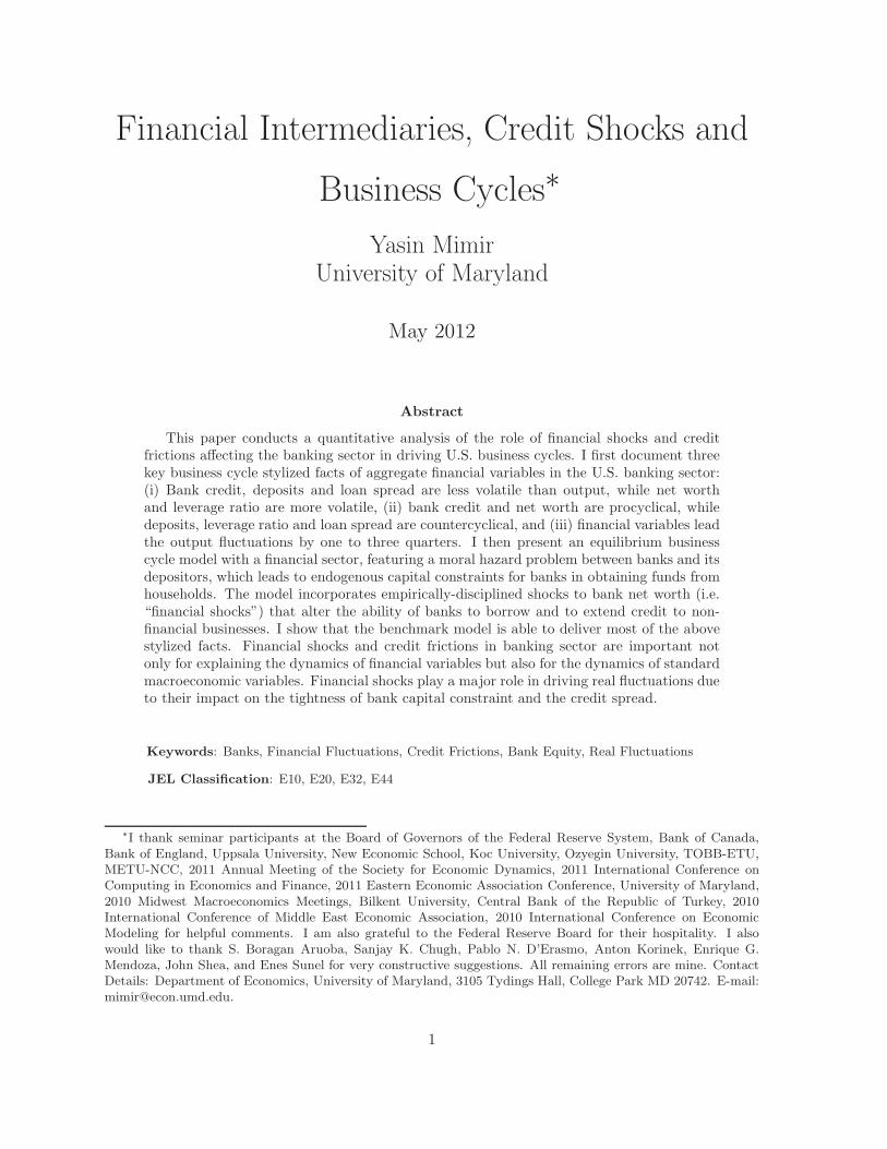
This section documents some key empirical features of financial cycles in the U.S. economy. The

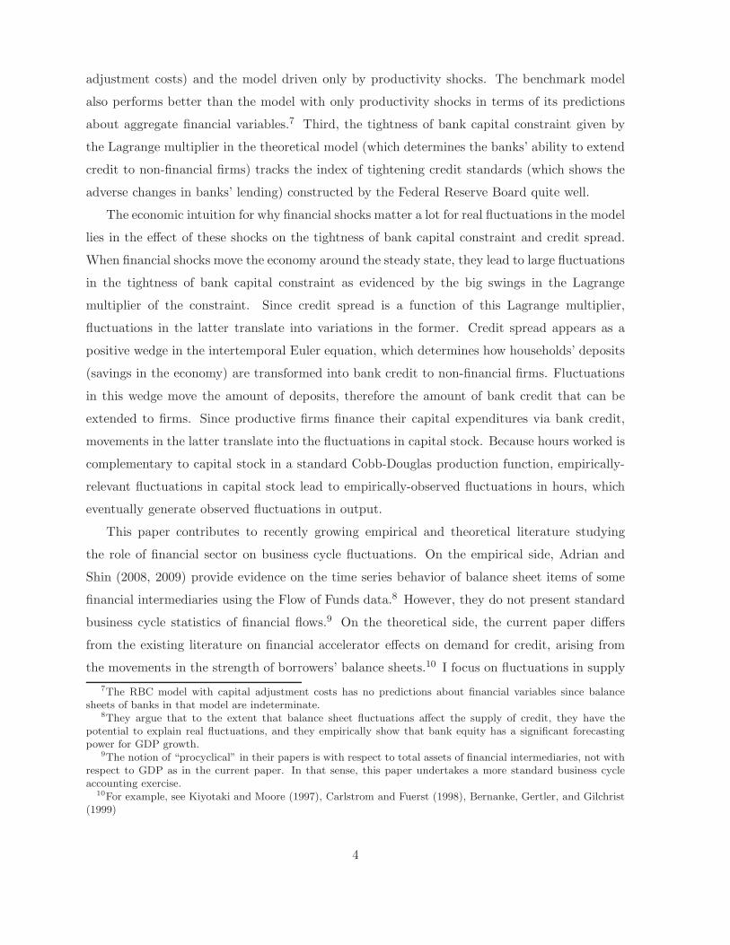
upper left panel of Figure 1 displays quarterly time series for loan losses of U.S. commercial

11The latter also features the interbank market.

5

banks from 1987 to 2010. The loan loss rates are expressed as annualized percentages of GDP.

The figure shows that loan loss rates increased in last three recessions of the U.S. economy.

The loss rates peaked in both 1990-91 and 2007-09 recessions, reaching its highest level of 5%

in the latter. The upper right panel of Figure 1 plots daily time series for Dow Jones Bank

Index from 1992 to 2010. The figure suggests that the market value of banks’ shares declined

substantially in the recent recession. Finally, the middle left panel of Figure 1 displays real

net worth growth of U.S. commercial banks (year-on-year). The figure suggests that banks’

net worth shrank in last three recessions of the U.S. economy, with a reduction of 40% in the

2007-09 recession. These three plots convey a common message: substantial loan losses incurred

by banks together with the fall in their equity prices typically cause large declines in banks’ net

worth, which might lead to persistent and mounting pressures on bank balance sheets, worsening

the aggregate credit conditions, and thus causing the observed decline in real economic activity,

which is much more pronounced in the Great Recession.

The middle left panel of Figure 1 plots commercial and industrial loan spreads over federal

funds rate (annualized). The figure shows that bank lending spreads sky-rocketed in the recent

crisis, reaching a 3.2% per annum towards the end of the recession and they keep rising although

the recession was officially announced to be over. The bottom left panel displays real bank credit

growth rates (year-on-year). The figure indicates that bank credit growth fell significantly in

the recent economic downturn. Taken together, these figures suggest that the U.S. economy

has experienced a significant deterioration in aggregate credit conditions as total bank lending

to non-financial sector declined sharply and the cost of funds for non-financial firms increased

substantially. Finally, the bottom right panel of Figure 1 plots real deposit growth rates (year-

on-year). The figure shows that growth rate of deposits began to fall substantially right after

the recent recession.

I will assess the performance of the model below by its ability to match empirical cyclical

properties of real and financial variables in the U.S data. Table 1 presents the business cycle

properties of aggregate financial variables in U.S. commercial banking sector together with

standard macro aggregates for the period 1987-2010.12 The correlation coefficients in bold

font are the maximum ones in their respective rows, which indicate the lead-lag relationship of

variables with output. The aggregate financial variables I consider are U.S. commercial banks’

12I focus on the period that begins in 1987 for two reasons. First, U.S. banking sector witnessed a significanttransformation starting from 1987 such as deregulation of deposit rates, increases in financial flexibility. Second,it also corresponds to a structural break in the volatility of many standard macro variables, which is so-calledGreat Moderation.

6

0

1

2

3

4

5

88 90 92 94 96 98 00 02 04 06 08 10

Loan losses to GDP ratio

0

100

200

300

400

500

600

92 94 96 98 00 02 04 06 08 10

Dow Jones bank index

-60

-40

-20

0

20

40

60

88 90 92 94 96 98 00 02 04 06 08 10

Net worth growth

1.5

2.0

2.5

3.0

3.5

88 90 92 94 96 98 00 02 04 06 08 10

Interest rate spreads

-8

-4

0

4

8

12

88 90 92 94 96 98 00 02 04 06 08 10

Bank credit

-2

0

2

4

6

8

10

88 90 92 94 96 98 00 02 04 06 08 10

Deposit growth

Figure 1: Financial Flows in the U.S. Economy

7

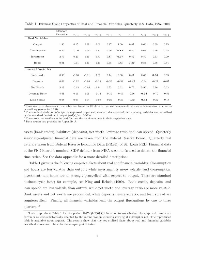
Table 1: Business Cycle Properties of Real and Financial Variables, Quarterly U.S. Data, 1987- 2010

Standard

Deviation xt−4 xt−3 xt−2 xt−1 xt xt+1 xt+2 xt+3 xt+4

Real Variables

Output 1.80 0.15 0.39 0.66 0.87 1.00 0.87 0.66 0.39 0.15

Consumption 0.45 -0.20 0.06 0.37 0.66 0.82 0.80 0.67 0.46 0.25

Investment 2.73 0.27 0.49 0.71 0.87 0.97 0.82 0.59 0.33 0.09

Hours 0.91 -0.01 0.19 0.43 0.65 0.83 0.89 0.83 0.68 0.44

Financial Variables

Bank credit 0.93 -0.20 -0.11 0.02 0.14 0.30 0.47 0.63 0.68 0.63

Deposits 0.69 -0.02 -0.08 -0.18 -0.30 -0.39 -0.42 -0.34 -0.22 -0.07

Net Worth 5.17 -0.15 -0.03 0.14 0.32 0.52 0.70 0.80 0.76 0.63

Leverage Ratio 5.61 0.16 0.05 -0.12 -0.30 -0.49 -0.66 -0.74 -0.70 -0.55

Loan Spread 0.08 0.05 0.04 -0.08 -0.21 -0.39 -0.42 -0.43 -0.32 -0.18

a Business cycle statistics in the table are based on HP-filtered cyclical components of quarterly empirical time series(smoothing parameter:1600).b The standard deviation of output is expressed in percent; standard deviations of the remaining variables are normalizedby the standard deviation of output (std(x)/std(GDP)).c The correlation coefficients in bold font are the maximum ones in their respective rows.d Data sources are provided in Appendix A.

assets (bank credit), liabilities (deposits), net worth, leverage ratio and loan spread. Quarterly

seasonally-adjusted financial data are taken from the Federal Reserve Board. Quarterly real

data are taken from Federal Reserve Economic Data (FRED) of St. Louis FED. Financial data

at the FED Board is nominal. GDP deflator from NIPA accounts is used to deflate the financial

time series. See the data appendix for a more detailed description.

Table 1 gives us the following empirical facts about real and financial variables. Consumption

and hours are less volatile than output, while investment is more volatile; and consumption,

investment, and hours are all strongly procyclical with respect to output. These are standard

business-cycle facts; for example, see King and Rebelo (1999). Bank credit, deposits, and

loan spread are less volatile than output, while net worth and leverage ratio are more volatile.

Bank assets and net worth are procyclical, while deposits, leverage ratio, and loan spread are

countercyclical. Finally, all financial variables lead the output fluctuations by one to three

quarters.13

13I also reproduce Table 1 for the period 1987:Q1-2007:Q1 in order to see whether the empirical results aredriven or at least substantially affected by the recent economic events starting at 2007:Q3 or not. The reproducedtable is available upon request. The results show that the key stylized facts about real and financial variablesdescribed above are robust to the sample period taken.

8

Table 2: The Sequence of Events in a Given Time Period

1. Productivity zt is realized.2. Firms hire labor Ht and use capital Kt they purchased in period t− 1, which are used for production, Yt = ztF(Kt, Ht).3. Firms make their wage payments wtHt and dividend payments to shareholders (banks) from period t-1.4. Banks make their interest payments on deposits of households from period t-1 and bankers exit with probability (1-θ).5. Recovery rate ωt is realized.6. Households make their consumption and saving decisions and deposit their resources at banks.7. Firms sell their depreciated capital to capital producers. These agents make investment and produce new capital Kt+1.8. Firms issue shares [st = Kt+1] and sell these shares to banks to finance their capital expenditures.9. Banks purchase firms’ shares and their incentive constraints bind.10. Firms purchase capital Kt+1 from capital producers at the price of qt with borrowed funds.

3 A Business Cycle Model with Financial Sector

The model is an otherwise standard real business cycle model with a financial sector. Credit

frictions in financial sector are modeled as in Gertler and Karadi (2011). I introduce shocks to

bank net worth on top of the standard productivity shocks. The model economy consists of four

types of agents: households, financial intermediaries, firms, and capital producers. The ability

of financial intermediaries to borrow from households is limited due to a moral hazard (costly

enforcement) problem, which will be described below. Firms acquire capital in each period by

selling shares to financial intermediaries. Finally, capital producers are incorporated into the

model in order to introduce capital adjustment costs in a tractable way. Table 2 shows the

sequence of events in a given time period in the theoretical model described below. The section

below will clarify this timeline.

3.1 Households

There is a continuum of identical households of measure unity. Households are infinitely-lived

with preferences over consumption (ct) and leisure (1 − Lt) given by

E0

∞∑

t=0

βtU(ct, 1 − Lt) (1)

Each household consumes and supplies labor to firms at the market clearing real wage wt.

In addition, they save by holding deposits at a riskless real return rt at competitive financial

intermediaries.

There are two types of members within each household: workers and bankers. Workers

supply labor and return the wages they earn to the household while each banker administers a

financial intermediary and transfers any earnings back to the household. Hence, the household

owns the financial intermediaries that its bankers administer. However, the deposits that the

9

household holds are put in financial intermediaries that it doesn’t own.14 Moreover, there is

perfect consumption insurance within each household.

At any point in time the fraction 1 − ζ of the household members are workers and the re-

maining fraction ζ are bankers. An individual household member can switch randomly between

these two jobs over time. A banker this period remains a banker next period with probability θ,

which is independent of the banker’s history. Therefore, the average survival time for a banker

in any given period is 1/(1− θ). The bankers are not infinitely-lived in order to make sure that

they don’t reach a point where they can finance all equity investment from their own net worth.

Hence, every period (1 − θ)ζ bankers exit and become workers while the same mass of workers

randomly become bankers, keeping the relative proportion of workers and bankers constant.

Period t bankers learn about survival and exit at the beginning of period t + 1. Bankers who

exit from the financial sector transfer their accumulated earnings to their respective household.

Furthermore, the household provides its new bankers with some start-up funds.15

The household budget constraint is given by

ct + bt+1 = wtLt + (1 + rt)bt + Πt (2)

The household’s subjective discount factor is β ∈ (0,1), ct denotes the household’s consump-

tion, bt+1 is the total amount of deposits that the household gives to the financial intermediary,

rt is the non-contingent real return on the deposits from t− 1 to t, wt is the real wage rate, and

Πt is the profits to the household from owning capital producers and banks net of the transfer

that it gives to its new bankers plus (minus) the amount of wealth redistributed from banks

(households) to households (banks).

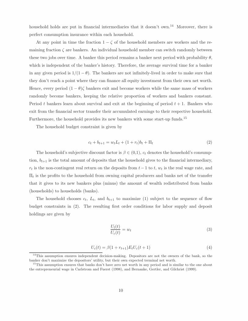
The household chooses ct, Lt, and bt+1 to maximize (1) subject to the sequence of flow

budget constraints in (2). The resulting first order conditions for labor supply and deposit

holdings are given by

Ul(t)

Uc(t)= wt (3)

Uc(t) = β(1 + rt+1)EtUc(t + 1) (4)

14This assumption ensures independent decision-making. Depositors are not the owners of the bank, so thebanker don’t maximize the depositors’ utility, but their own expected terminal net worth.

15This assumption ensures that banks don’t have zero net worth in any period and is similar to the one aboutthe entrepreneurial wage in Carlstrom and Fuerst (1998), and Bernanke, Gertler, and Gilchrist (1999).

10

The first condition states that the marginal rate of substitution between consumption and

leisure is equal to the wage rate. The second condition is the standard consumption-savings

Euler equation, which equates the marginal cost of not consuming and saving today to the

expected discounted marginal benefit of consuming tomorrow.

3.2 Financial Intermediaries

3.2.1 Balance Sheets

Financial intermediaries transfer the funds that they obtain from households to firms. They

acquire firm shares and finance these assets with household deposits and their own equity.

At the beginning of period t, before banks collect deposits, an aggregate net worth shock hits

banks’ balance sheets. Let’s denote ωt as the time-varying recovery rate of loans as a percentage

of bank net worth. Innovations to ωt are shocks to bank net worth. Therefore, ωtnjt is the

effective net worth of the financial intermediary. For notational convenience, I denote ωtnjt by

njt. Hence, njt is the net worth of financial firm j at the beginning of period t after the net

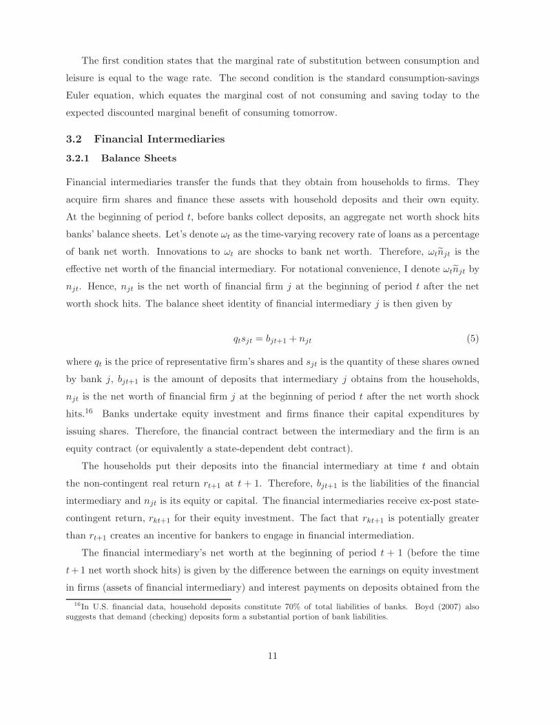
worth shock hits. The balance sheet identity of financial intermediary j is then given by

qtsjt = bjt+1 + njt (5)

where qt is the price of representative firm’s shares and sjt is the quantity of these shares owned

by bank j, bjt+1 is the amount of deposits that intermediary j obtains from the households,

njt is the net worth of financial firm j at the beginning of period t after the net worth shock

hits.16 Banks undertake equity investment and firms finance their capital expenditures by

issuing shares. Therefore, the financial contract between the intermediary and the firm is an

equity contract (or equivalently a state-dependent debt contract).

The households put their deposits into the financial intermediary at time t and obtain

the non-contingent real return rt+1 at t + 1. Therefore, bjt+1 is the liabilities of the financial

intermediary and njt is its equity or capital. The financial intermediaries receive ex-post state-

contingent return, rkt+1 for their equity investment. The fact that rkt+1 is potentially greater

than rt+1 creates an incentive for bankers to engage in financial intermediation.

The financial intermediary’s net worth at the beginning of period t + 1 (before the time

t+ 1 net worth shock hits) is given by the difference between the earnings on equity investment

in firms (assets of financial intermediary) and interest payments on deposits obtained from the

16In U.S. financial data, household deposits constitute 70% of total liabilities of banks. Boyd (2007) alsosuggests that demand (checking) deposits form a substantial portion of bank liabilities.

11

households (liabilities of financial intermediary). Thus the law of motion for bank net worth is

given by

njt+1 = (1 + rkt+1)qtsjt − (1 + rt+1)bjt+1 (6)

Using the balance sheet of the financial firm given by (5), we can re-write (6) as follows:

njt+1 = (rkt+1 − rt+1)qtsjt + (1 + rt+1)njt (7)

The financial intermediary’s net worth at time t+ 1 depends on the premium rkt+1 − rt+1 that

it earns on shares purchased as well as the total value of these shares, qtsjt.

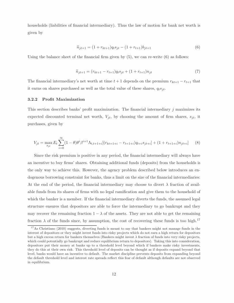
3.2.2 Profit Maximization

This section describes banks’ profit maximization. The financial intermediary j maximizes its

expected discounted terminal net worth, Vjt, by choosing the amount of firm shares, sjt, it

purchases, given by

Vjt = maxsjt

Et

∞∑

i=0

(1 − θ)θiβi+1Λt,t+1+i[(rkt+1+i − rt+1+i)qt+isjt+i] + (1 + rt+1+i)njt+i] (8)

Since the risk premium is positive in any period, the financial intermediary will always have

an incentive to buy firms’ shares. Obtaining additional funds (deposits) from the households is

the only way to achieve this. However, the agency problem described below introduces an en-

dogenous borrowing constraint for banks, thus a limit on the size of the financial intermediaries:

At the end of the period, the financial intermediary may choose to divert λ fraction of avail-

able funds from its shares of firms with no legal ramification and give them to the household of

which the banker is a member. If the financial intermediary diverts the funds, the assumed legal

structure ensures that depositors are able to force the intermediary to go bankrupt and they

may recover the remaining fraction 1 − λ of the assets. They are not able to get the remaining

fraction λ of the funds since, by assumption, the cost of recovering these funds is too high.17

17As Christiano (2010) suggests, diverting funds is meant to say that bankers might not manage funds in theinterest of depositors or they might invest funds into risky projects which do not earn a high return for depositorsbut a high excess return for bankers themselves (Bankers might invest λ fraction of funds into very risky projects,which could potentially go bankrupt and reduce equilibrium return to depositors). Taking this into consideration,depositors put their money at banks up to a threshold level beyond which if bankers make risky investments,they do this at their own risk. This threshold level of deposits can be thought as if deposits expand beyond thatlevel, banks would have an incentive to default. The market discipline prevents deposits from expanding beyondthe default threshold level and interest rate spreads reflect this fear of default although defaults are not observedin equilibrium.

12

Therefore, for the banks not to have an incentive to divert the funds, the following incentive

compatibility constraint must be satisfied at the end of period t:

Vjt ≥ λqtsjt (9)

The left-hand side of (9) is the value of operating for the bank (or equivalently cost of

diverting funds) while the right-hand side is the gain from diverting λ fraction of assets. The

intuition for this constraint is that in order for the financial intermediary not to divert the funds

and for the households to put their deposits into the bank, the value of operating in financial

sector must be greater than or equal to the gain from diverting assets.

A financial intermediary’s objective is to maximize the expected return to its portfolio

consisting of firms’ shares and its capital subject to the incentive compatibility constraint.

Then its demand for shares is fully determined by its net worth position, since as long as the

expected return from the portfolio is strictly positive, it will expand its lending (its size) until

the incentive compatibility constraint binds.

3.2.3 Leverage Ratio and Net Worth Evolution

Proposition 1 The expected discounted terminal net worth of a bank can be expressed as the sum

of expected discounted total return to its equity investment into firms and expected discounted

total return to its existing net worth.

Proof : See Appendix B.1

Proposition 1 states that that Vjt can be expressed as follows:

Vjt = νtqtsjt + ηtnjt (10)

where

νt = Et[(1 − θ)βΛt,t+1(rkt+1 − rt+1) + βΛt,t+1θqt+1sjt+1

qtsjtνt+1] (11)

ηt = Et[(1 − θ)βΛt,t+1(1 + rt+1) + βΛt,t+1θnjt+1

njtηt+1] (12)

νt can be interpreted as the expected discounted marginal gain to the bank of buying one

more unit of firms’ shares, holding its net worth njt constant. The first term is the discounted

value of the net return on shares to the bank if it exits the financial sector tomorrow. The

second term is the continuation value of its increased assets if it survives. Meanwhile, ηt can be

13

interpreted as the expected discounted marginal benefit of having one more unit of net worth,

holding qtsjt constant. The first term is the discounted value of the return on net worth to the

bank if it exits the financial sector tomorrow. The second term is the continuation value of its

increased net worth if it survives.

Therefore, we can write the incentive compatibility constraint as follows:

νtqtsjt + ηtnjt ≥ λqtsjt (13)

Proposition 2 The incentive compatibility constraint binds as long as 0 < νt < λ.

Proof : I prove this by contradiction. Assume that νt ≥ λ. Then the left-hand side of (13) is

always greater than the right-hand side of (13) since ηtnjt > 0 as can be seen from (12). The

franchise value of the bank is always higher than the gain from diverting funds. Therefore, the

constraint is always slack. Moreover, assume that νt ≤ 0. Since νt is the expected discounted

marginal gain to the bank of increasing its assets, the intermediary does not have the incentive

to expand its assets when νt ≤ 0. In this case, the constraint does not bind because the

intermediary does not collect any deposits from households.

The profits of the financial intermediary will be affected by the premium rkt+1− rt+1 . That

is, the banker will not have any incentive to buy firms’ shares if the discounted return on these

shares is less than the discounted cost of deposits. Thus the financial firm will continue to

operate in period t + i if the following inequality is satisfied:

Et+iβΛt,t+1+i(rkt+1+i − rt+1+i) ≥ 0 ∀i ≥ 0 (14)

where βΛt,t+1+i is the stochastic discount factor that the financial firm applies to its earnings

at t + 1 + i. The moral hazard problem between households and banks described above limits

banks’ ability to obtain deposits from the households, leading to a positive premium. The

following proposition establishes this fact.

Proposition 3 Risk premium is positive as long as the incentive compatibility constraint binds.

Proof : See Appendix B.2

When this constraint binds, the financial intermediary’s assets are limited by its net worth.

That is, if this constraint binds, the funds that the intermediary can obtain from households

will depend positively on its equity capital:

qtsjt =ηt

λ− νtnjt (15)

14

The constraint (15) limits the leverage of the financial intermediary to the point where

its incentive to divert funds is exactly balanced by its loss from doing so. Thus, the costly

enforcement problem leads to an endogenous borrowing constraint on the bank’s ability to

acquire assets. When bank’s leverage ratio and/or bank equity is high, it can extend more

credit to non-financial firms. Conversely, de-leveraging or the deterioration in net worth in bad

times will limit the bank’s ability to extend credit. Note that by manipulating this expression

using the balance sheet, I can obtain the bank’s leverage ratio as follows:

bjt+1

njt=

ηtλ− νt

− 1 (16)

The leverage ratio increases in the expected marginal benefit of buying one more unit of

firm share, and in the expected marginal gain of having one more unit of net worth. Intuitively,

increases in ηt or νt mean that financial intermediation is expected to be more lucrative going

forward, which makes it less attractive to divert funds today and thus increases the amount of

funds depositors are willing to entrust to the financial intermediary.18

Using (15), I can re-write the law of motion for the banker’s net worth as follows:

njt+1 = [(rkt+1 − rt+1)ηt

λ− νt+ (1 + rt+1)]njt (17)

The sensitivity of net worth of the financial intermediary j at t+1 to the ex-post realization

of the premium rkt+1 − rt+1 increases in the leverage ratio.

Proposition 4 Banks have an identical leverage ratio as none of its components depends on

bank-specific factors.

Proof : From (17), one can obtain the following:

njt+1

njt= [(rkt+1 − rt+1)

ηtλ− νt

+ (1 + rt+1)] (18)

qt+1sjt+1

qtsjt=

ηt+1

λ−νt+1

ηtλ−νt

njt+1

njt(19)

The expressions above show that banks have identical expected growth rates of assets and

18The amount of deposits at banks does directly depend on banks’ net worth. In good times banks’ net worthis relatively high and depositors believe that bankers do not misbehave in terms of managing their funds properly.In these times, credit spreads can be fully explained by observed bankruptcies and intermediation costs. However,in bad times, banks experience substantial declines in their net worth and depositors are hesitant about puttingtheir money in banks. In these times, the financial sector operates at a less efficient level and a smaller numberof investment projects are funded. Large credit spread observed in these times can be explained by the abovefactors plus the inefficiency in the banking system.

15

net worth, thus have identical leverage ratios.19

By using Proposition 4, we can sum demand for assets across j to obtain the total interme-

diary demand for assets:

qtst =ηt

λ− νtnt (20)

where st is the aggregate amount of assets held by financial intermediaries and nt is the aggregate

intermediary net worth. In the equilibrium of the model, movements in the leverage ratio of

financial firms and/or in their net worth will generate fluctuations in total intermediary assets.

The aggregate intermediary net worth at the beginning of period t + 1 (before the net

worth shock hits but after exit and entry), nt+1, is the sum of the net worth of surviving

financial intermediaries from the previous period, net+1, and the net worth of entering financial

intermediaries, nnt+1. Thus, we have

nt+1 = net+1 + nnt+1 (21)

Since the fraction θ of the financial intermediaries at time t will survive until time t + 1,

their net worth, net+1, is given by

net+1 = θ[(rkt+1 − rt+1)ηt

λ− νt+ (1 + rt+1)]nt (22)

Newly entering financial intermediaries receive start-up funds from their respective house-

holds. The start-up funds are assumed to be a transfer equal to a fraction of the net worth

of exiting bankers. The total final period net worth of exiting bankers at time t is equal to

(1 − θ)nt. The household is assumed to transfer the fraction ǫ(1−θ) of the total final period net

worth to its newly entering financial intermediaries. Therefore, we have

nnt+1 = ǫnt (23)

Using (21), (22), and (23), we obtain the following law of motion for nt+1:

nt+1 = θ[(rkt+1 − rt+1)ηt

λ− νt+ (1 + rt+1)]nt + ǫnt (24)

19This immediately implies that ηt and νt are independent of j. In Appendix B.1, I use this result in explicitderivation of ηt and νt.

16

3.3 Firms

There is a continuum of unit mass of firms that produce the final output in the economy. The

production technology at time t is described by the constant returns to scale function:

Yt = ztF (Kt,Ht) = ztKαt H

1−αt (25)

where Kt is the firm’s capital stock, Ht is the firm’s hiring of labor and zt is an aggregate TFP

realization.

Firms acquire capital Kt+1 at the end of period t to produce the final output in the next

period. After producing at time t + 1, the firm can sell the capital on the open market.

Firms finance their capital expenditures in each period by issuing equities and selling them

to financial intermediaries. Firms issue st units of state-contingent claims (equity), which is

equal to the number of units of capital acquired Kt+1. The financial contract between a financial

intermediary and a firm is an equity contract (or equivalently, a state contingent debt contract).

The firm pays a state-contingent interest rate equal to the ex-post return on capital rkt+1 to

the financial intermediary. The firms set their capital demand Kt+1 taking this stochastic

repayment into consideration. At the beginning of period t+1 (after shocks are realized), when

output becomes available, firms obtain resources Yt+1 and use them to make repayments to

shareholders (or financial intermediaries). The firm prices each financial claim at the price of a

unit of capital, qt. Thus, we have

qtst = qtKt+1 (26)

There are no frictions for firms in obtaining funds from financial intermediaries. The bank

has perfect information about the firm and there is perfect enforcement. Therefore, in the

current model, only banks face endogenous borrowing constraints in obtaining funds. These

constraints directly affect the supply of funds to the firms.

Firms choose the labor demand at time t as follows:

wt = ztFH(Kt,Ht) (27)

Then firms pay out the ex-post return to capital to the banks given that they earn zero

profit state by state. Therefore, ex-post return to capital is given by

rkt+1 =zt+1FK(Kt+1,Ht+1) + qt+1(1 − δ)

qt− 1 (28)

17

Labor demand condition (27) simply states that the wage rate is equal to the marginal

product of labor. Moreover, condition (28) states that the ex-post real rate of return on capital

is equal to the marginal product of capital plus the capital gain from changed prices.

3.4 Capital Producers

Following the literature on financial accelerator, I incorporate capital producers into the model

in order to introduce capital adjustment costs in a tractable way. Capital adjustment costs are

needed to introduce some variation in the price of capital; otherwise the price of capital will

not respond to the changes in capital stock and will always be equal to 1.20

I assume that households own capital producers and receive any profits. At the end of period

t, competitive capital producers buy capital from firms to repair the depreciated capital and to

build new capital. Then they sell both the new and repaired capital. The cost of replacing the

depreciated capital is unity; thus the price of a unit of new capital or repaired capital is qt. The

profit maximization problem of the capital producers is given by:

maxIt

qtKt+1 − qt(1 − δ)Kt − It (29)

s.t. Kt+1 = (1 − δ)Kt + Φ

(ItKt

)Kt (30)

where It) is the total investment by capital producing firms and Φ(

ItKt

)is the capital adjustment

cost function. The resulting optimality condition gives the following “Q” relation for investment:

qt =

[Φ

′

(ItKt

)]−1

(31)

where Φ′

(ItKt

)is the partial derivative of the capital adjustment cost function with respect

to investment-capital ratio at time t. The fluctuations in investment expenditures will create

variation in the price of capital. A fall in investment at time t (ceteris paribus) will reduce the

price of capital in the same period.

I leave the definition of the competitive equilibrium of the model to Appendix C.

20There will be no financial accelerator between households and banks if there is no variation in the price ofcapital.

18

4 Quantitative Analysis

This section studies the quantitative predictions of the model by examining the results of nu-

merical simulations of an economy calibrated to quarterly U.S. data. In order to investigate the

dynamics of the model, I compute a second-order approximation to the equilibrium conditions

using Dynare.

4.1 Functional Forms, Parametrization and Calibration

The quantitative analysis uses the following functional forms for preferences, production tech-

nology and capital adjustment costs:21

U(c, 1 − L) = log(c) + υ(1 − L) (32)

F (K,H) = KαH1−α (33)

Φ

(I

K

)=

I

K−

ϕ

2

[I

K− δ

]2(34)

Table 4 lists the parameter values for the model economy. The preference and production

parameters are standard in business cycle literature. I take the quarterly discount factor, β as

0.9942 to match the 2.37% average annualized real deposit rate in the U.S. I pick the relative

utility weight of labor υ as 1.72 to fix hours worked in steady state, L, at one third of the

available time. The share of capital in the production function is set to 0.36 to match the

labor share of income in the U.S. data. The capital adjustment cost parameter is taken so as

to match the relative volatility of price of investment goods with respect to output in the U.S.

data.22 The quarterly depreciation rate of capital is set to 2.25% to match the average annual

investment to capital ratio.

The non-standard parameters in our model are the financial sector parameters: the fraction

of the revenues that can be diverted, λ, the proportional transfer to newly entering bankers,

ǫ, and the survival probability of bankers, θ. I set ǫ to 0.001 so that the proportional trans-

fer to newly entering bankers is 0.1% of aggregate net worth.23 I pick other two parameters

21I choose the functional form of the capital adjustment cost following Bernanke, Gertler and Gilchrist (1999),Gertler, Gilchrist, and Natalucci (2007) etc.

22The volatility of price of investment goods is taken from Gomme et al. (2011).23I keep the proportional transfer to newly entering bankers small, so that it does not have significant impact

on the results.

19

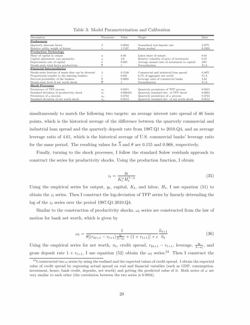
Table 3: Model Parameterization and Calibration

Description Parameter Value Target Data

Preferences

Quarterly discount factor β 0.9942 Annualized real deposit rate 2.37%Relative utility weight of leisure υ 1.7167 Hours worked 0.3333Production Technology

Share of capital in output α 0.36 Labor share of output 0.64Capital adjustment cost parameter ϕ 3.6 Relative volatility of price of investment 0.37Depreciation rate of capital δ 0.025 Average annual ratio of investment to capital 10%Steady-state total factor productivity z 1 Normalization N/AFinancial Intermediaries

Steady-state fraction of assets that can be diverted λ 0.1548 Commercial and industrial loan spread 0.46%Proportional transfer to the entering bankers ǫ 0.001 0.1% of aggregate net worth N/ASurvival probability of the bankers θ 0.9685 Leverage ratio of commercial banks 4.62Steady-state level of net worth shock ω 1 Normalization N/AShock Processes

Persistence of TFP process ρz 0.9315 Quarterly persistence of TFP process 0.9315Standard deviation of productivity shock σz 0.006424 Quarterly standard dev. of TFP shock 0.0064Persistence of ω process ρω 0.3744 Quarterly persistence of ω process 0.3744Standard deviation of net worth shock σω 0.0512 Quarterly standard dev. of net worth shock 0.0512

simultaneously to match the following two targets: an average interest rate spread of 46 basis

points, which is the historical average of the difference between the quarterly commercial and

industrial loan spread and the quarterly deposit rate from 1987.Q1 to 2010.Q4, and an average

leverage ratio of 4.61, which is the historical average of U.S. commercial banks’ leverage ratio

for the same period. The resulting values for λ and θ are 0.155 and 0.968, respectively.

Finally, turning to the shock processes, I follow the standard Solow residuals approach to

construct the series for productivity shocks. Using the production function, I obtain

zt =yt

Kαt H

1−αt

(35)

Using the empirical series for output, yt, capital, Kt, and labor, Ht, I use equation (51) to

obtain the zt series. Then I construct the log-deviation of TFP series by linearly detrending the

log of the zt series over the period 1987.Q1-2010.Q4.

Similar to the construction of productivity shocks, ωt series are constructed from the law of

motion for bank net worth, which is given by

ωt =1

θ[(rkt+1 − rt+1) ηtλ−νt

+ (1 + rt+1)] + ǫ

nt+1

nt(36)

Using the empirical series for net worth, nt, credit spread, rkt+1 − rt+1, leverage, ηtλ−νt

, and

gross deposit rate 1 + rt+1, I use equation (52) obtain the ωt series.24 Then I construct the

24I constructed two ω series by using the realized and the expected values of credit spread. I obtain the expectedvalue of credit spread by regressing actual spread on real and financial variables (such as GDP, consumption,investment, hours, bank credit, deposits, net worth) and getting the predicted value of it. Both series of ω arevery similar to each other (the correlation between the two series is 0.9934).

20

-.06

-.04

-.02

.00

.02

.04

88 90 92 94 96 98 00 02 04 06 08 10

Level of productivity

-.2

-.1

.0

.1

.2

.3

88 90 92 94 96 98 00 02 04 06 08 10

Level of omega

-.03

-.02

-.01

.00

.01

.02

88 90 92 94 96 98 00 02 04 06 08 10

Innovations to productivity

-.2

-.1

.0

.1

.2

.3

88 90 92 94 96 98 00 02 04 06 08 10

Innovations to omega

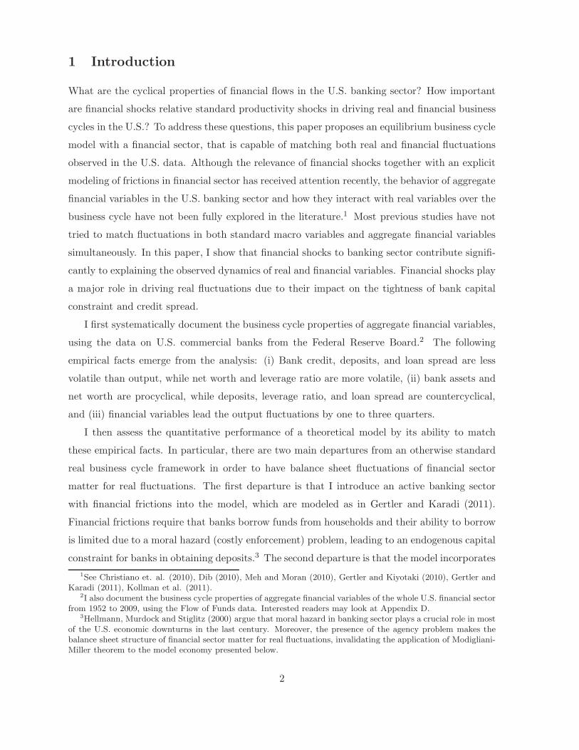
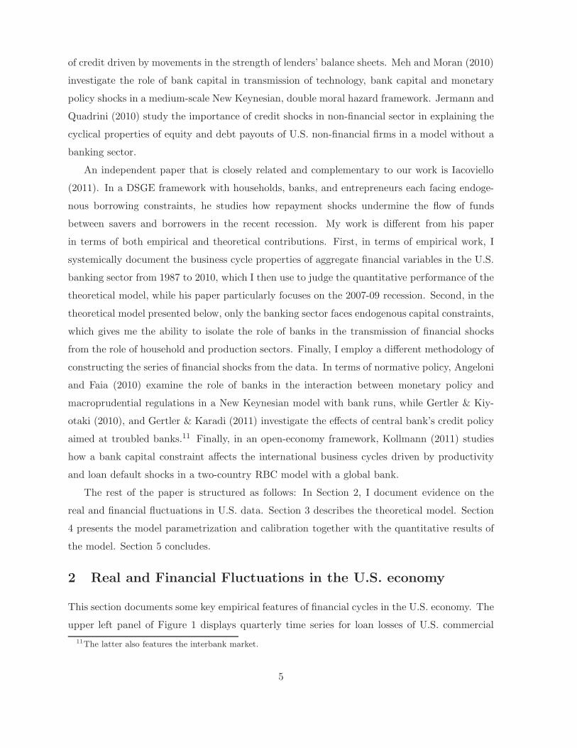
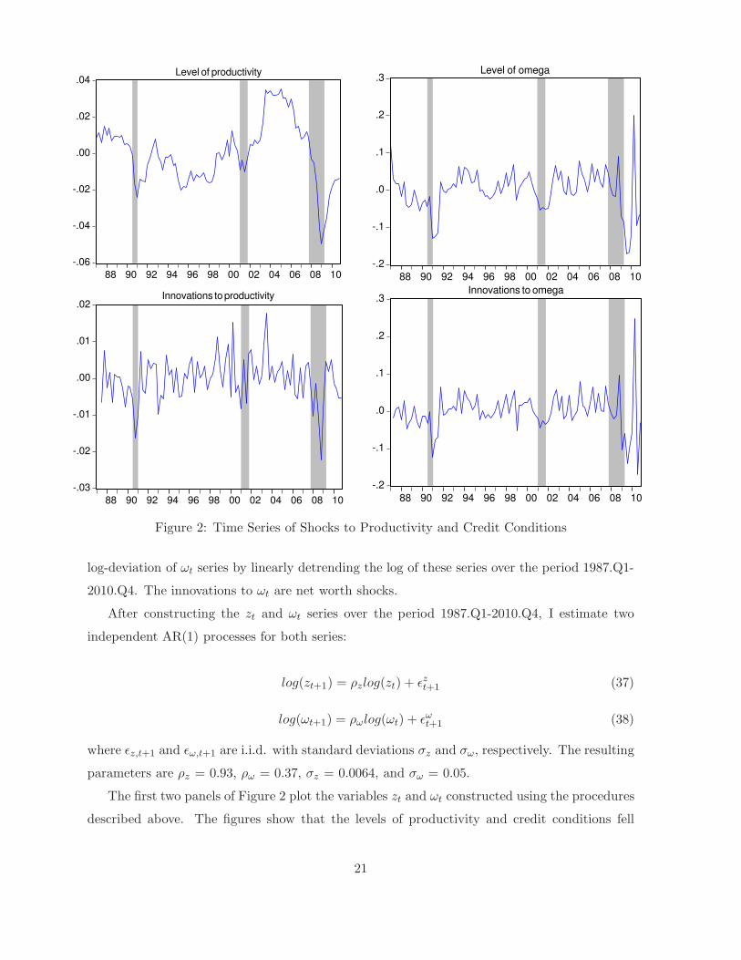
Figure 2: Time Series of Shocks to Productivity and Credit Conditions

log-deviation of ωt series by linearly detrending the log of these series over the period 1987.Q1-

2010.Q4. The innovations to ωt are net worth shocks.

After constructing the zt and ωt series over the period 1987.Q1-2010.Q4, I estimate two

independent AR(1) processes for both series:

log(zt+1) = ρzlog(zt) + ǫzt+1 (37)

log(ωt+1) = ρωlog(ωt) + ǫωt+1 (38)

where ǫz,t+1 and ǫω,t+1 are i.i.d. with standard deviations σz and σω, respectively. The resulting

parameters are ρz = 0.93, ρω = 0.37, σz = 0.0064, and σω = 0.05.

The first two panels of Figure 2 plot the variables zt and ωt constructed using the procedures

described above. The figures show that the levels of productivity and credit conditions fell

21

sharply in the recent recession. The bottom panels plot the innovations ǫz,t and ǫω,t. These

innovations are unexpected changes in the levels of productivity and financial conditions. The

plots suggest that the U.S. economy is severely hit by both negative productivity and financial

shocks in the Great Recession.

0 0.1 0.2 0.3 0.40.8

1

1.2

1.4

1.6Output

0 0.1 0.2 0.3 0.40.7

0.8

0.9

1Consumption

0 0.1 0.2 0.3 0.40.1

0.2

0.3

0.4

0.5Investment

0 0.1 0.2 0.3 0.40.3

0.32

0.34

0.36Hours

0 0.1 0.2 0.3 0.40

5

10

15Deposits

0 0.1 0.2 0.3 0.40

1

2

3Net Worth

0 0.1 0.2 0.3 0.40

5

10

15

20Leverage Ratio

0 0.1 0.2 0.3 0.40

0.5

1

1.5Credit Spread (%)

0 0.1 0.2 0.3 0.45

10

15

20Total Credit

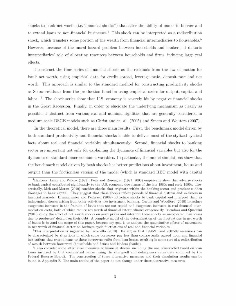
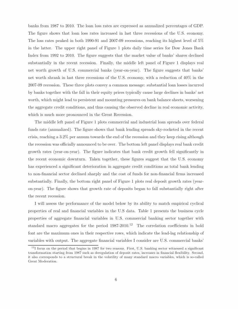
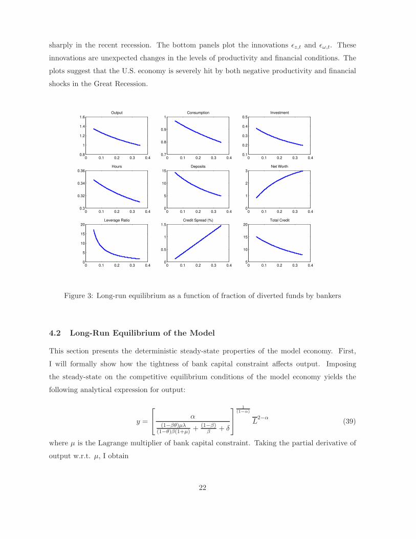
Figure 3: Long-run equilibrium as a function of fraction of diverted funds by bankers

4.2 Long-Run Equilibrium of the Model

This section presents the deterministic steady-state properties of the model economy. First,

I will formally show how the tightness of bank capital constraint affects output. Imposing

the steady-state on the competitive equilibrium conditions of the model economy yields the

following analytical expression for output:

y =

α

(1−βθ)µλ(1−θ)β(1+µ) + (1−β)

β+ δ

1(1−α)

L2−α

(39)

where µ is the Lagrange multiplier of bank capital constraint. Taking the partial derivative of

output w.r.t. µ, I obtain

22

∂y

∂µ= −

α

(1 − α)

α

(1−βθ)µλ(1−θ)β(1+µ) + (1−β)

β+ δ

α(1−α)

L2−α

[(1 − θ)β(1 − βθ)λ

[(1 − θ)β(1 + µ)]2

]−2

< 0 (40)

which unambiguously shows that the output will be lower the larger µ. The reason is simple.

As the bank capital constraint gets tighter, the credit spread will be larger, as can be seen from

the following expression.

(rk − r) =(1 − βθ)µλ

(1 − θ)β(1 + µ)(41)

The term at the right-hand side of equation (57) appears as a positive wedge in the intertemporal

Euler equation, which determines how deposits (savings) are transformed into credit to firms

in the economy. This positive wedge reduces the amount of savings that can be extended as

credit to non-financial firms, lowering their physical capital accumulation, and thus leading to a

lower steady-state output. The same mechanism is also at work when shocks move the economy

around the steady-state as they tighten or relax the bank capital constraint.

Second, I analytically show how output is affected by the severity of credit frictions in

banking sector, which is governed by the fraction of diverted funds by bankers, λ. Taking the

partial derivative of output w.r.t. λ, I get

∂y

∂λ= −

αL2−α

(1 − α)

α[(1−βθ)[(1−ǫ)β−θ](1−θ)β(1−ǫ)β

] (1−α)α

(1−βθ)[(1−ǫ)β−θ]λ(1−θ)β(1−ǫ)β + (1−β)+βδ

β

α(1−α) [

(1 − βθ)[(1 − ǫ)β − θ]λ

(1 − θ)β(1 − ǫ)β+

(1 − β) + βδ

β

]−2

< 0

(42)

which implies that the steady-state output will be lower the higher the intensity of financial

frictions in banking sector. In order to get the intuition behind this result, I display long-run

equilibria of real and financial variables as a function of the intensity of the credit friction in the

financial sector given by fraction of diverted funds by bankers, λ. All other parameter values

are set to those shown in Table 3. Figure 3 shows that the long-run dynamics of the model

economy to changes in λ is monotonic and non-linear. As λ increases, households’ incentive to

make deposits into banks falls since the bankers’ gain from diverting funds rises. Banks have

to finance their equity investment by internal financing rather than external financing. Thus,

deposits go down and net worth rises, leading to a fall in banks’ leverage ratio. The decline

in leverage ratio is sharper than the rise in net worth, inducing a drop in total credit to non-

financial firms. Credit conditions tighten for firms and their cost of funds given by credit spread

23

goes up. This leads to a reduction in investment and output falls.

4.3 Intermediary Capital and the Transmission of Shocks

I present the dynamics of the model in response to productivity and net worth shocks. In the

figures below, credit spread, return to capital, and deposit rate are expressed in percentage

points per annum. The responses of all other variables are expressed in percentage deviations

from their respective steady state values.

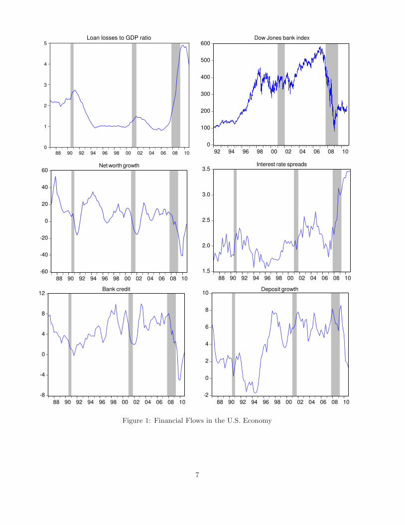
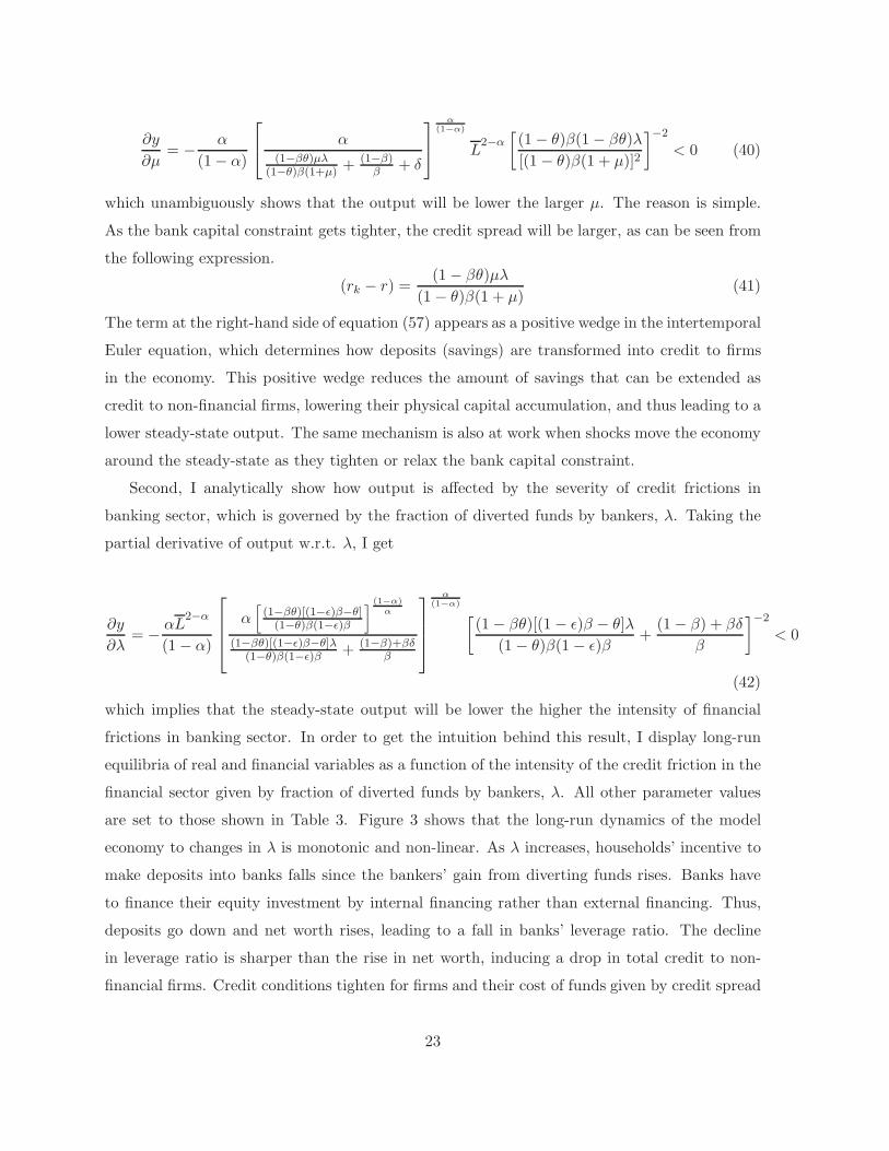
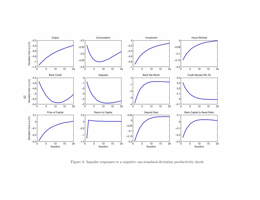
Figure 4 presents the impulse responses to a one-time, one-standard deviation negative

shock to TFP. The negative technology shock reduces the price of investment goods produced

by capital producers by 0.3% on impact, lowering the value of firms’ shares. This makes purchase

of their shares less profitable for banks, which can also be observed from the 1.2% fall in the

return to capital. Thus, banks have difficulty in obtaining deposits from households since their

equity investment becomes less attractive. This reduces the return to deposits by 0.2%, inducing

a countercyclical credit spread. The spread rises by 0.3% on impact. In order to compensate the

fall in their external financing, banks need to finance a larger share of their purchases of equities

from their net worth. However, bank net worth also falls by 4% due to lower asset prices. Since

the decline in net worth is sharper than the fall in deposits on impact, banks’ leverage ratio

rises. Hence, the model with productivity shocks generates a countercyclical leverage ratio.

Because banks cannot adjust their net worth immediately and the lower price of capital reduces

the value of their net worth, their financing conditions tighten and bank lending in the form of

equity purchases falls dramatically (by about 4.6%), inducing aggregate investment to shrink

by 0.9%. Finally, hours fall by 0.15%, and output declines by 1.2%.

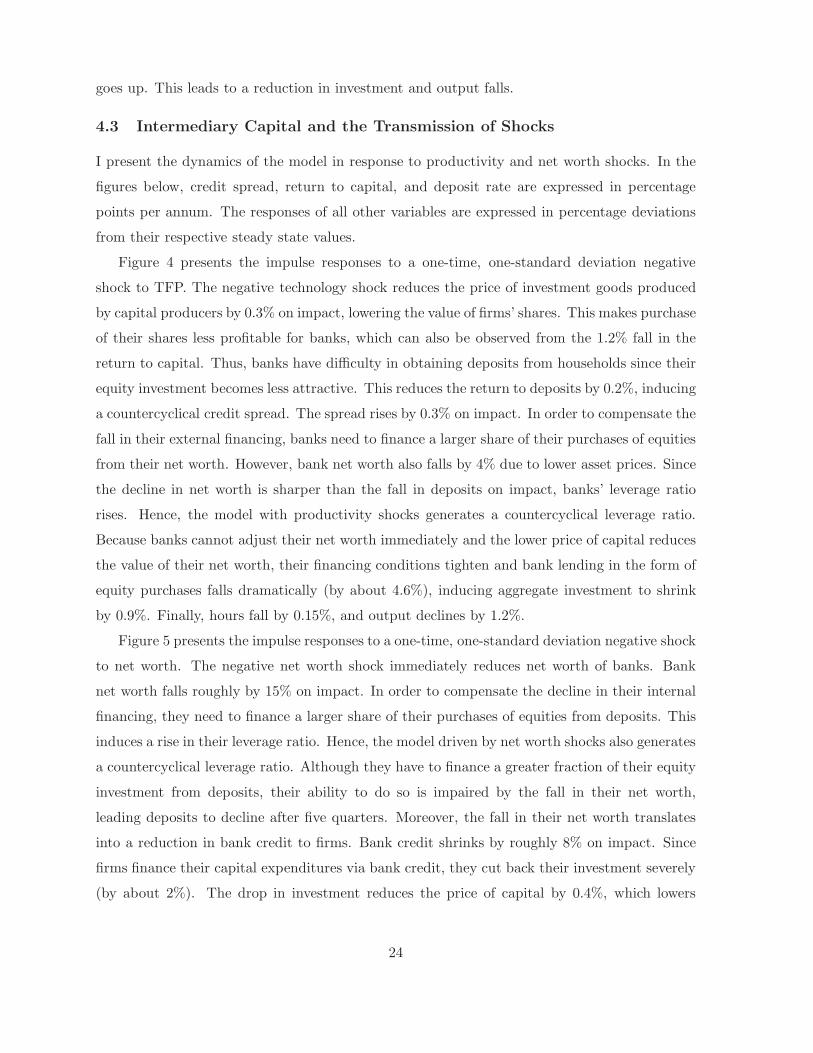
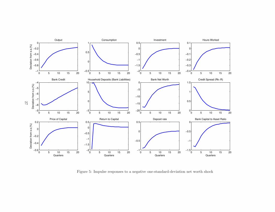
Figure 5 presents the impulse responses to a one-time, one-standard deviation negative shock

to net worth. The negative net worth shock immediately reduces net worth of banks. Bank

net worth falls roughly by 15% on impact. In order to compensate the decline in their internal

financing, they need to finance a larger share of their purchases of equities from deposits. This

induces a rise in their leverage ratio. Hence, the model driven by net worth shocks also generates

a countercyclical leverage ratio. Although they have to finance a greater fraction of their equity

investment from deposits, their ability to do so is impaired by the fall in their net worth,

leading deposits to decline after five quarters. Moreover, the fall in their net worth translates

into a reduction in bank credit to firms. Bank credit shrinks by roughly 8% on impact. Since

firms finance their capital expenditures via bank credit, they cut back their investment severely

(by about 2%). The drop in investment reduces the price of capital by 0.4%, which lowers

24

banks’ net worth further. Hours fall by 0.4% and output drops by 0.9% on impact. Finally,

consumption rises on impact after the shock hits, which is what was observed at the beginning

of the recent financial crisis. In the context of the model, this seemingly unappealing result

can be explained as follows: On the intratemporal margin, the fall in aggregate demand caused

by lower investment expenditures translates into a reduction in the demand for labor, which

eventually leads to a drop in hours worked. Since wages are flexible, the reduction in labor

demand also lowers wages, leading to a fall in households’ wage bill. However, the rise in credit

spread on impact raises banks’ profits. Since households own banks, the rise in their profits

helps households sustain their consumption after the financial shock hits. On impact, the rise

in bank profits dominates the reduction in wage bill, pushing consumption up.25

25Barro and King (1984) argue that any shock that reduces the quantity of hours worked on impact has to leada fall in consumption due to consumption-leisure optimality condition. Ajello (2010) shows that sticky wages arethe key factor in generating a positive comovement between consumption and investment after a financial shock.

25

0 5 10 15 20−1.2

−1

−0.8

−0.6

−0.4

−0.2

Devia

tion f

rom

s.s

.(%

)

Output

0 5 10 15 20−0.4

−0.35

−0.3

−0.25

−0.2Consumption

0 5 10 15 20−1

−0.8

−0.6

−0.4

−0.2

0Investment

0 5 10 15 20−0.2

−0.15

−0.1

−0.05

0Hours Worked

0 5 10 15 20−5.4

−5.2

−5

−4.8

−4.6

−4.4

Devia

tion f

rom

s.s

.(%

)

Bank Credit

0 5 10 15 20−5

−4

−3

−2

−1

0Deposits

0 5 10 15 20−4

−3

−2

−1

0Bank Net Worth

0 5 10 15 20−0.1

0

0.1

0.2

0.3

0.4Credit Spread (Rk−R)

0 5 10 15 20−0.3

−0.2

−0.1

0

0.1

Quarters

Devia

tion fro

m s

.s.(

%)

Price of Capital

0 5 10 15 20−1.5

−1

−0.5

0

0.5

Quarters

Return to Capital

0 5 10 15 20−0.2

−0.15

−0.1

−0.05

0

0.05

Quarters

Deposit Rate

0 5 10 15 20−0.3

−0.2

−0.1

0

0.1

Quarters

Bank Capital to Asset Ratio

Figure 4: Impulse responses to a negative one-standard-deviation productivity shock

26

0 5 10 15 20−1

−0.8

−0.6

−0.4

−0.2

0

Devia

tion f

rom

s.s

.(%

)

Output

0 5 10 15 20−0.5

0

0.5

1Consumption

0 5 10 15 20−2

−1.5

−1

−0.5

0

0.5Investment

0 5 10 15 20−0.4

−0.3

−0.2

−0.1

0

0.1Hours Worked

0 5 10 15 20−9

−8

−7

−6

−5

−4

Devia

tion f

rom

s.s

.(%

)

Bank Credit

0 5 10 15 20−5

0

5

10Household Deposits (Bank Liabilities)

0 5 10 15 20−20

−15

−10

−5

0Bank Net Worth

0 5 10 15 200

0.5

1

1.5Credit Spread (Rk−R)

0 5 10 15 20−0.6

−0.4

−0.2

0

0.2

Quarters

Devia

tion fro

m s

.s.(

%)

Price of Capital

0 5 10 15 20−2

−1.5

−1

−0.5

0

0.5

Quarters

Return to Capital

0 5 10 15 20−1

−0.5

0

0.5

Quarters

Deposit rate

0 5 10 15 20−1.5

−1

−0.5

0

Quarters

Bank Capital to Asset Ratio

Figure 5: Impulse responses to a negative one-standard-deviation net worth shock

27

4.4 Business Cycle Dynamics

This section presents numerical results from stochastic simulations of the benchmark economy

with productivity and net worth shocks. First, I simulate the model economy 1000 times for

1096 periods each and discard the first 1000 periods in each simulation so that each simulation

has the same length as the data sample. I then compute the standard business cycle statistics

using the cyclical components of the HP-filtered series. I also conduct the same quantitative

exercise for the frictionless version of the benchmark economy, which is essentially the standard

RBC model with capital adjustment costs, in order to compare the real fluctuations in both

models. Finally, I simulate the model economy only driven by productivity shocks to see the

contribution of net worth shocks to the observed dynamics of real and financial variables.

Table 4 presents quarterly real and financial statistics in the data and in the model economies.

In particular, it displays the relative standard deviations of real and financial variables with

respect to output and their cross-correlations with output. Column 3 of the table shows that

the standard RBC model with capital adjustment costs driven by standard productivity shocks

is able produce the key business cycle facts in the U.S. data as expected: consumption and

hours less volatile than output, while investment is more volatile, all real variables are highly

procyclical. However, this model can only explain 80% of the fluctuations in output and less

than half of the relative volatility in hours. It also generates roughly perfect positive corre-

lation between real variables and output, contrary to the data. Moreover, this model has no

predictions about financial variables.

Column 4 of the table shows the business cycle statistics of our model economy with only

productivity shocks. This model is much closer to the data in terms of real fluctuations, com-

pared to the RBC model. It now accounts for 85% of the fluctuations in output and roughly half

of the relative volatility in hours. The model is also able to replicate most of the stylized facts

about financial variables: bank assets, deposits and loan spread is less volatile than output,

while net worth and leverage ratio are more volatile; bank assets and net worth are procycli-

cal, while leverage ratio and loan spread are countercyclical. However, it generates procyclical

deposits, contrary to the data. Although the model does a good job in terms of key facts of

financial variables, it predicts lower fluctuations. For example, it can explain less than half

of the relative volatility in bank assets, roughly half of the relative volatility in deposits, less

than one third of the relative volatility in net worth and leverage ratio. The model virtually

matches the relative volatility of credit spread. Column 5 of the table shows the real and fi-

nancial statistics in the benchmark economy driven by both shocks. This model is even closer

28

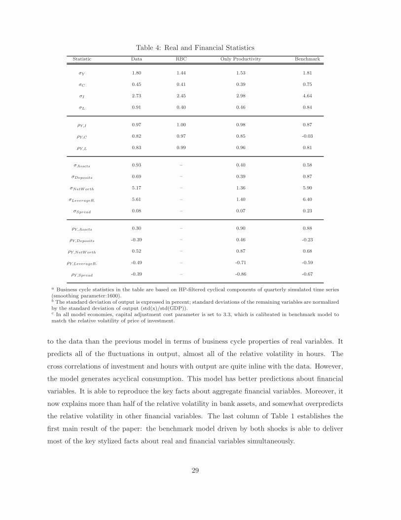
Table 4: Real and Financial Statistics

Statistic Data RBC Only Productivity Benchmark

σY 1.80 1.44 1.53 1.81

σC 0.45 0.41 0.39 0.75

σI 2.73 2.45 2.98 4.64

σL 0.91 0.40 0.46 0.84

ρY,I 0.97 1.00 0.98 0.87

ρY,C 0.82 0.97 0.85 -0.03

ρY,L 0.83 0.99 0.96 0.81

σAssets 0.93 – 0.40 0.58

σDeposits 0.69 – 0.39 0.87

σNetWorth 5.17 – 1.36 5.90

σLeverageR. 5.61 – 1.40 6.40

σSpread 0.08 – 0.07 0.23

ρY,Assets 0.30 – 0.90 0.88

ρY,Deposits -0.39 – 0.46 -0.23

ρY,NetWorth 0.52 – 0.87 0.68

ρY,LeverageR. -0.49 – -0.71 -0.59

ρY,Spread -0.39 – -0.86 -0.67

a Business cycle statistics in the table are based on HP-filtered cyclical components of quarterly simulated time series(smoothing parameter:1600).b The standard deviation of output is expressed in percent; standard deviations of the remaining variables are normalizedby the standard deviation of output (std(x)/std(GDP)).c In all model economies, capital adjustment cost parameter is set to 3.3, which is calibrated in benchmark model tomatch the relative volatility of price of investment.

to the data than the previous model in terms of business cycle properties of real variables. It

predicts all of the fluctuations in output, almost all of the relative volatility in hours. The

cross correlations of investment and hours with output are quite inline with the data. However,

the model generates acyclical consumption. This model has better predictions about financial

variables. It is able to reproduce the key facts about aggregate financial variables. Moreover, it

now explains more than half of the relative volatility in bank assets, and somewhat overpredicts

the relative volatility in other financial variables. The last column of Table 1 establishes the

first main result of the paper: the benchmark model driven by both shocks is able to deliver

most of the key stylized facts about real and financial variables simultaneously.

29

-16

-12

-8

-4

0

4

8

12

88 90 92 94 96 98 00 02 04 06 08 10

Data RBC Benchmark 1

GDP

corr(data, rbc) = 0.69

corr(data, benchmark 1) = 0.80

-50

-40

-30

-20

-10

0

10

20

30

88 90 92 94 96 98 00 02 04 06 08 10


Investment



-12

-8

-4

0

4

8

88 90 92 94 96 98 00 02 04 06 08 10


Hours



Figure 6: Real Fluctuations: Benchmark vs. RBC model

30

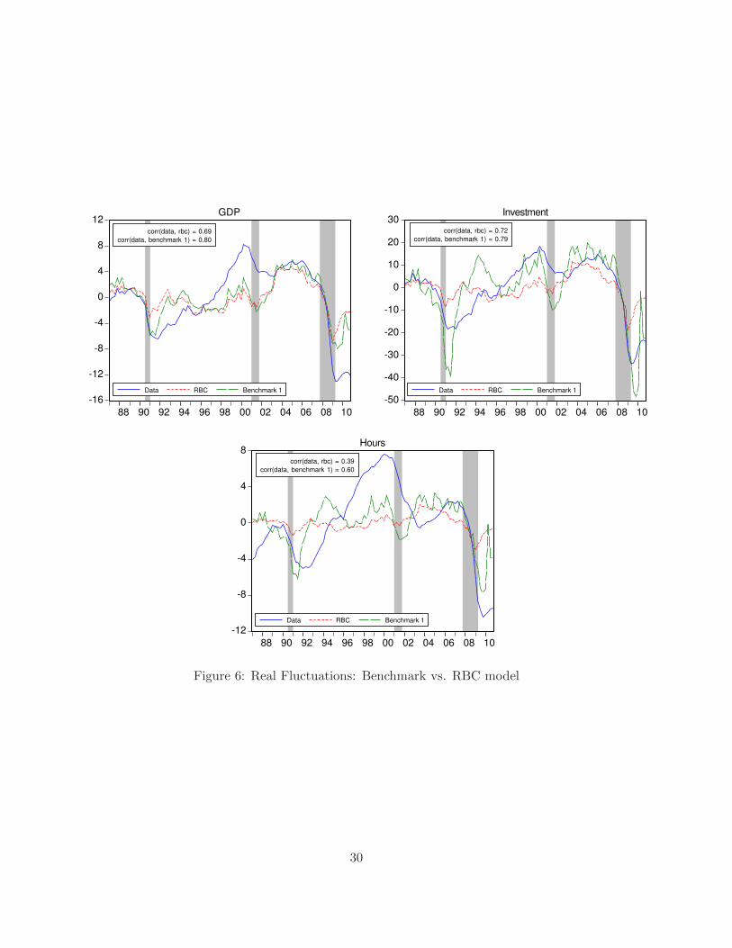
I also study the dynamics of the model in response to the actual sequence of shocks to see

whether the model is able to generate the real and financial cycles observed in the U.S. data.26

I basically feed the actual innovations to zt and ωt into the model and compute the responses

of real and financial variables over the period 1987 to 2010.

Figure 6 displays the quarterly time series of output, investment and hours in the data, in

the standard RBC model with capital adjustment costs, and in the benchmark economy. The

RBC model is driven by standard productivity shocks, while the benchmark model is driven by

both shocks. Both the quarterly times series of the variables and their model counterparts are

log-linearly detrended over the period 1987.Q1 - 2010.Q4, and plotted in percentage deviations

from their trends. The correlations between the actual and the model-simulated series are also

reported in the graphs. The figure suggests that both the RBC model and the benchmark econ-

omy generate series of real variables that closely follow their empirical counterparts. However,

the RBC model predicts lower fluctuations in all real variables. In particular, the RBC model

predicts a smaller decline in output in the 1990-91 recession. Moreover, it generates declines

in investment and hours that are smaller than the actual declines in the 1990-91 and 2007-09

recessions. On the other hand, the benchmark model generates larger fluctuations in real vari-

ables, consistent with the data. Since this model has one additional shock compared to the

RBC model, higher volatility can be expected. However, the benchmark model also improves

upon the RBC model in the sense that for all real variables, the cross-correlations between

the data and the benchmark model is much higher than those between the data and the RBC

model. Moreover, the model’s success in generating empirically-relevant fluctuations in hours

hinges on the fact that it is able to produce quantitatively reasonable fluctuations in capital.

Since labor is complementary to capital stock in a standard Cobb-Douglas production function,

empirically-relevant changes in capital stock lead to observed fluctuations in hours.

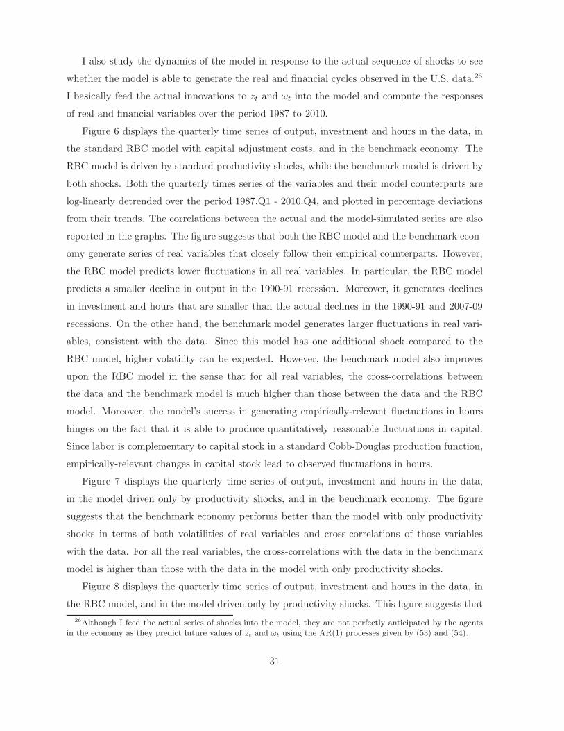
Figure 7 displays the quarterly time series of output, investment and hours in the data,

in the model driven only by productivity shocks, and in the benchmark economy. The figure

suggests that the benchmark economy performs better than the model with only productivity

shocks in terms of both volatilities of real variables and cross-correlations of those variables

with the data. For all the real variables, the cross-correlations with the data in the benchmark

model is higher than those with the data in the model with only productivity shocks.

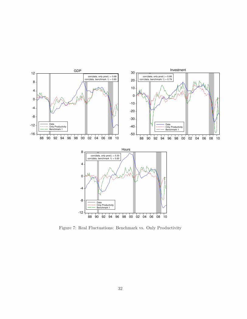
Figure 8 displays the quarterly time series of output, investment and hours in the data, in

the RBC model, and in the model driven only by productivity shocks. This figure suggests that

26Although I feed the actual series of shocks into the model, they are not perfectly anticipated by the agentsin the economy as they predict future values of zt and ωt using the AR(1) processes given by (53) and (54).

31

-16

-12

-8

-4

0

4

8

12

88 90 92 94 96 98 00 02 04 06 08 10

DataOnly ProductivityBenchmark 1

GDP

corr(data, only prod.) = 0.68


-50

-40

-30

-20

-10

0

10

20

30

88 90 92 94 96 98 00 02 04 06 08 10


Investment



-12

-8

-4

0

4

8

88 90 92 94 96 98 00 02 04 06 08 10


Hours



Figure 7: Real Fluctuations: Benchmark vs. Only Productivity

32

-16

-12

-8

-4

0

4

8

12

88 90 92 94 96 98 00 02 04 06 08 10

DataRBCOnly Productivity

GDP



-40

-30

-20

-10

0

10

20

88 90 92 94 96 98 00 02 04 06 08 10


Investment



-12

-8

-4

0

4

8

88 90 92 94 96 98 00 02 04 06 08 10


Hours



Figure 8: Real Fluctuations: RBC vs. Only Productivity

33

the model with only productivity shocks is not very different from the RBC model in terms of

its quantitative performance in real variables. Actually, the series of real variables generated by

these two models are almost the same. Therefore, we can say that credit frictions in banking

sector by themselves are not enough to improve upon the RBC model and to produce real

fluctuations consistent with the data. Financial shocks are quite important in explaining the

observed dynamics of real variables.

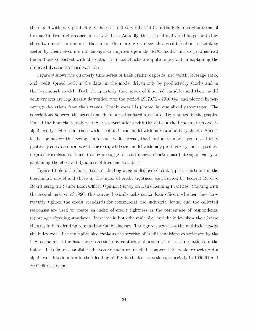
Figure 9 shows the quarterly time series of bank credit, deposits, net worth, leverage ratio,

and credit spread both in the data, in the model driven only by productivity shocks and in

the benchmark model. Both the quarterly time series of financial variables and their model

counterparts are log-linearly detrended over the period 1987.Q1 - 2010.Q4, and plotted in per-

centage deviations from their trends. Credit spread is plotted in annualized percentages. The

correlations between the actual and the model-simulated series are also reported in the graphs.

For all the financial variables, the cross-correlations with the data in the benchmark model is

significantly higher than those with the data in the model with only productivity shocks. Specif-

ically, for net worth, leverage ratio and credit spread, the benchmark model produces highly

positively correlated series with the data, while the model with only productivity shocks predicts

negative correlations. Thus, this figure suggests that financial shocks contribute significantly to

explaining the observed dynamics of financial variables.

Figure 10 plots the fluctuations in the Lagrange multiplier of bank capital constraint in the

benchmark model and those in the index of credit tightness constructed by Federal Reserve

Board using the Senior Loan Officer Opinion Survey on Bank Lending Practices. Starting with

the second quarter of 1990, this survey basically asks senior loan officers whether they have

recently tighten the credit standards for commercial and industrial loans, and the collected

responses are used to create an index of credit tightness as the percentage of respondents,

reporting tightening standards. Increases in both the multiplier and the index show the adverse

changes in bank lending to non-financial businesses. The figure shows that the multiplier tracks

the index well. The multiplier also explains the severity of credit conditions experienced by the

U.S. economy in the last three recessions by capturing almost most of the fluctuations in the

index. This figure establishes the second main result of the paper: U.S. banks experienced a

significant deterioration in their lending ability in the last recessions, especially in 1990-91 and

2007-09 recessions.

34

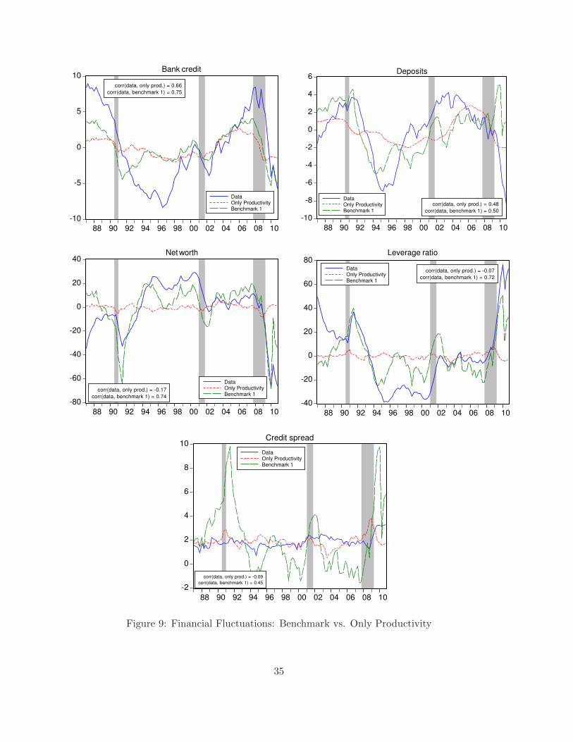
-10

-5

0

5

10

88 90 92 94 96 98 00 02 04 06 08 10


Bank credit



-10

-8

-6

-4

-2

0

2

4

6

88 90 92 94 96 98 00 02 04 06 08 10


Deposits



-80

-60

-40

-20

0

20

40

88 90 92 94 96 98 00 02 04 06 08 10


Net worth

corr(data, only prod.) = -0.17


-40

-20

0

20

40

60

80

88 90 92 94 96 98 00 02 04 06 08 10


Leverage ratio



-2

0

2

4

6

8

10

88 90 92 94 96 98 00 02 04 06 08 10


Credit spread



Figure 9: Financial Fluctuations: Benchmark vs. Only Productivity

35

-60

-40

-20

0

20

40

60

80

100

88 90 92 94 96 98 00 02 04 06 08 10

Survey of senior officersLagrange multiplier

Index of tightening credit standards

Figure 10: Tightness of Credit Conditions in the Benchmark Model

5 Conclusion

This paper quantitatively investigates the joint role of financial shocks and credit frictions

affecting banking sector in driving the real and financial fluctuations in the data. To this end, I

first characterize the empirical cyclical behavior of aggregate financial variables of U.S. banking

sector. I then use an otherwise standard real business cycle model with a simple financial sector,

which features an agency problem between banks and their depositors, leading to endogenous

borrowing constraints for banks in obtaining funds from households. I incorporate empirically-

disciplined shocks to bank net worth (i.e. “financial shocks”) which affect the ability of banks

to obtain funds from households and to extend credit to non-financial sector.The time series

of financial shocks are constructed from the data. The resulting shock series show that credit

conditions in the U.S. economy deteriorated significantly in the recent recession.

Several key findings emerge from the quantitative analysis. First, the benchmark model

driven by both productivity and financial shocks is able to explain most of the empirical facts

about real and financial variables simultaneously. Second, financial shocks to banking sector

contribute significantly not only to the observed dynamics of aggregate financial variables but

also to the observed dynamics of standard macroeconomic variables. In particular, the bench-

mark model has better predictions about real and financial variables than the model driven

only by productivity shocks. Third, the simulation of the benchmark model points a significant

36

worsening in banks’ lending ability in 1990-91 and 2007-09 recessions. The main transmission

mechanism of financial shocks is through bank capital channel. In particular, financial shocks

are transmitted to the real economy through tightening bank capital constraint, which eventu-

ally leads to rising credit spread. Non-financial firms perceive this rise in credit spread as an

increase in their cost of borrowing from banks, leading to a decline in their external finance

for investment expenditures. Falling aggregate demand caused by lower investment reduces the

demand for labor, which brings a drop in hours worked, and hence output.

For further research, one can investigate the normative implications of the model in the light

of the recent financial crisis, as U.S. government has assisted many financial firms in order to

raise their franchise value, and hence to support real economic activity. In order to start thinking

about how different policy tools can be implemented in an environment in which the financial

sector is crucial for business cycle fluctuations and what the welfare implications of these policies

are, I need a model capable of matching real and financial fluctuations simultaneously. I think

that the model proposed in this paper is quite successful in this dimension.

37

References

[1] Adrian, T., Shin, H.S., 2008. “Liquidity and Leverage.” Journal of Financial Intermedia-

tion, Vol.19 (3), pp. 418-437.

[2] Adrian, T., Shin, H.S., 2009. “Financial Intermediaries and Monetary Economics.” Federal

Reserve Bank of New York Staff Reports, No. 398.

[3] Ajello, A. 2010. “Financial Intermediation, Investment Dynamics and Business Cycle Fluc-

tuations.” Unpublished manuscript, Northwestern University.

[4] Angeloni, I., Faia, E., 2010. “Capital Regulation and Monetary Policy with Fragile Banks.”

Unpublished manuscript, European Central Bank.

[5] Barro, R., King, R., 1984. “Time-Separable Preferences and Intertemporal-Substitution

Models of Business Cycles.” The Quarterly Journal of Economics, pp. 817-839.

[6] Bernanke, B.S., Gertler M., Gilchrist, S., 1999. “The Financial Accelerator in a Quanti-

tative Business Cycle Framework.” In Handbook of Macroeconomics, edited by John B.

Taylor and Michael Woodford, Vol. 1C. Elsevier.

[7] Boyd, J.H., 2007. “Financial Intermediation.” The New Palgrave Dictionary of Economics

Online.

[8] Brunnermeier, M.K. and Pedersen, L.H., 2009. “Market Liquidity and Funding Liquidity.”

The Review of Financial Studies Vol. 22 (6), pp. 2201-2238.

[9] Carlson, M.A., King, T.B., Lewis, K.F., 2008. “Distress in the Financial Sector and Eco-

nomic Activity.” Finance and Economics Discussion Series, Federal Reserve Board, Wash-

ington, D.C., 2008-43.

[10] Carlstrom, C.T., Fuerst, T.S., 1998. “Agency Costs, Net Worth, and Business Fluctuations:

A Computable General Equilibrium Analysis.” American Economic Review, Vol.87, pp.

893-910.

38

[11] Carlstrom, C.T., Fuerst, T.S., 1998. “Agency Costs and Business Cycles.” Economic The-

ory, Vol.12, pp. 583-597.

[12] Christiano, L.J., Eichenbaum M. and Evans, C.L., 2005. “Nominal Rigidities and the Dy-

namic Effects of a Shock to Monetary Policy.” Journal of Political Economy Vol. 113 (1),

pp. 1-45.

[13] Christiano, L., 2010. “Remarks on Unconventional Monetary Policy.” IJCB Conference,

Bank of Japan.

[14] Chugh, S., 2010. “Firm Risk and Leverage Based Business Cycles.” Unpublished

manuscript, University of Maryland.

[15] Covas, F., Den Haan, W.J., 2011. “The Cyclical Behavior of Debt and Equity Finance.”

American Economic Review, forthcoming.

[16] Gertler, M., Gilchrist, S., Natalucci, F.M., 2007. “External Constraints on Monetary Policy

and the Financial Accelerator.” Journal of Money, Credit, and Banking, Vol. 39(2-3), pp.

295-330.

[17] Gertler, M., Karadi, P., 2011. “A Model of Unconventional Monetary Policy.” Journal of

Monetary Economics. forthcoming.

[18] Gertler, M., Kiyotaki, N. 2010. “Financial Intermediation and Credit Policy in Business

Cycle Analysis.” Unpublished manuscript, Princeton University.

[19] Gertler, M., Kiyotaki, N., Queralto, A. 2011. “Financial Crisis, Bank Risk Exposure and

Government Financial Policy.” Unpublished manuscript, New York University and Prince-

ton University.

[20] Gilchrist, S., Yankov V., Zakrajsek, E., 2010. “Credit Market Shocks and Economic Fluc-

tuations: Evidence from Corporate Bond and Stock Markets.” Journal of Monetary Eco-

nomics, forthcoming.

[21] Gilchrist, S., Zakrajsek, E., 2011. “Monetary Policy and Credit Supply Shocks.” IMF

Economic Review, forthcoming.

39

[22] Gomme, P., Ravikumar, B., Rupert, P., 2011. “The Return to Capital and the Business

Cycle.” Review of Economic Dynamics, Vol.14, pp. 262-278.

[23] Hancock, D., Laing, A.J. and Wilcox, J.A., 1995. “Bank Capital Shocks: Dynamics Effects

on Securities, Loans and Capital.” Journal of Banking & Finance Vol. 19 (3-4), pp. 661-677.

[24] Hellmann, T.F., Murdock, K.C., Stiglitz, J.E., 2000. “Liberalization, Moral Hazard in

Banking, and Prudential Regulation: Are Capital Requirements Enough?.” American Eco-

nomic Review, Vol.90(1), pp. 147-165.

[25] Holmstrom B., Tirole, J., 1997. “Financial Intermediation, Loanable Funds and the Real

Sector.” Quarterly Journal of Economics, Vol.112, pp. 663-691.

[26] Iacoviello, M., 2010. “Financial Business Cycles.” Unpublished manuscript, Federal Reserve

Board.

[27] IMF, 2010. “Global Financial Stability Report (April 2010).” International Monetary Fund.

[28] Jeanne, O., Korinek, A., 2009. “Managing Credit Booms and Busts: A Pigouvian Taxation

Approach.” Unpublished manuscript, University of Maryland.

[29] Jermann, U., Quadrini, V., 2010. “Macroeconomic Effects of Financial Shocks.” American

Economic Review, forthcoming.

[30] Kiyotaki, N., Moore, J., 1997. “Credit Cycles.” Journal of Political Economy, Vol.105, pp.

211-248.

[31] Kollmann, R., Enders, Z., Muller, G.J., 2011. “Global Banking and International Business

Cycles.” European Economic Review, Vol.55, pp. 407-426.

[32] Korajczyk, R.A., Levy, A., 2003. “Capital Structure Choice: Macroeconomic Conditions

and Financial Constraints.” Journal of Financial Economics, Vol.68, pp. 75-109.

[33] Levin, A.T., Natalucci, F.M., Zakrajsek, E., 2004. “The Magnitude and Cyclical Behavior

of Financial Market Frictions.” Finance and Discussion Series, Federal Reserve Board of

Governors, No.70.

40

[34] Meh, C., Moran, K., 2010. “The Role of Bank Capital in the Propagation of Shocks.”

Journal of Economic Dynamics and Control, Vol.34, pp. 555-576.

[35] Mendoza, E.G., Quadrini, V., 2010. “Financial Globalization, Financial Crises and Conta-

gion.” Journal of Monetary Economics, Vol.57, pp. 24-39.

[36] Schmitt-Grohe, S., Uribe, M., 2004. “Solving Dynamic General Equilibrium Models Using

a Second-Order Approximation to the Policy Function.” Journal of Economic Dynamics

and Control, Vol.28, pp. 755-775.

[37] Smets, F. and Wouters, R., 2007. “Shocks and Frictions in US Business Cycles: A Bayesian

DSGE Approach.” American Economic Review, Vol.97 (3), pp. 586-606.

[38] Woodford, M., Curdia, V., 2010. “Credit Spreads and Monetary Policy.” Journal of Money,

Credit and Banking, forthcoming.

41

Appendix A: Data Appendix

Quarterly seasonally-adjusted data on standard macroeconomic variables except Hours are

taken from the Federal Reserve Economic Data (FRED) of St. Louis FED. Hours data are

taken from Current Employment Statistics survey published by the Bureau of Labor Statis-

tics. GDP deflator from NIPA accounts is used to deflate the time series of the nominal macro

aggregates. Consumption is the sum of “Personal consumption expenditures on nondurables”

(PCND) and “Personal consumption expenditures on services”. Investment is the sum of “Per-

sonal consumption expenditures on durables” (PCDG) and “Gross private domestic investment”

(GPDI). GDP is the sum of Consumption and Investment. Hours is computed as the multipli-

cation of “average weekly hours in private sector” with “average number of workers in private

sector”. Quarterly time series of capital stock to obtain zt series are constructed using the

approach described in the online appendix of Jermann and Quadrini (2010).

Quarterly financial time series of Bank assets and Bank liabilities are constructed using the

monthly data on Assets and Liabilities of Commercial Banks in the U.S. from Data Download

Program of Statistical & Historical Database of the Federal Reserve Board. Financial data

at the FED board are seasonally-adjusted but nominal. GDP deflator from NIPA accounts

is used to deflate the financial time series. Bank assets are bank credit at the asset side of

the balance sheet of the U.S. commercial banks. Bank liabilities are deposits held at the U.S.

commercial banks. Quarterly time series of Loan spread are taken from Survey of Terms of

Business Lending from Statistical & Historical Database of the FED Board. Loan spread is

commercial and industrial loan spread over intended federal funds rate. Quarterly deposit rates

are constructed using monthly data on 3-month certificate of deposit secondary market rate

from FRED. The inflation rate computed from GDP deflator is used to make nominal deposit

rate data real.

42

Appendix B

B.1. Proof of Proposition 1

Let’s conjecture that the bank’s franchise value is given by

Vjt = νtqtsjt + ηtnt (43)

Comparing the conjectured solution for Vjt to the expected discounted terminal net worth yields

the following expressions,

νtqtsjt = Et

∞∑

i=0

(1 − θ)θiβi+1Λt,t+1+i[(rkt+1+i − rt+1+i)qt+isjt+i] (44)

ηtnjt = Et

∞∑

i=0

(1 − θ)θiβi+1Λt,t+1+i(1 + rt+1+i)njt+i (45)

I write νt and ηt recursively using the expression above. Let’s begin with νt. To ease the

notation, let’s drop expectations for now.

νt =

∞∑

i=0

(1 − θ)θiβi+1Λt,t+1+i [(rkt+1+i − rt+1+i)xt,t+i] (46)

where xt,t+i =qt+isjt+i

qtsjt.

νt = (1 − θ)βΛt,t+1(rkt+1 − rt+1) +

∞∑

i=1

(1 − θ)θiβi+1Λt,t+1+i [(rkt+1+i − rt+1+i)xt,t+i] (47)

νt = (1−θ)βΛt,t+1(rkt+1−rt+1)+βΛt,t+1θxt,t+1

∞∑

i=0

(1−θ)θi+1βi+1Λt+1,t+2+i [(rkt+2+i − rt+2+i)xt+1,t+1+i]

(48)

The infinite sum at the right-hand side of equation (64) is one period updated version of equation

(62), given by

νt+1 =

∞∑

i=0

(1 − θ)θi+1βi+1Λt+1,t+2+i [(rkt+2+i − rt+2+i)xt+1,t+1+i] (49)

where xt+1,t+1+i =qt+1+isjt+1+i

qt+1sjt+1.

Hence, we can re-write (64) with the expectations as follows:

νt = Et[(1 − θ)βΛt,t+1(rkt+1 − rt+1) + βΛt,t+1θxt,t+1νt+1] (50)

43

Let’s continue with ηt. To ease the notation, let’s drop expectations for now.

ηt =

∞∑

i=0

(1 − θ)θiβi+1Λt,t+1+i(1 + rt+1+i)zt,t+i (51)

where zt,t+i =njt+i

njt

ηt = (1 − θ)βΛt,t+1(1 + rt+1) +

∞∑

i=1

(1 − θ)θiβi+1Λt,t+1+i(1 + rt+1+i)zt,t+i (52)

ηt = (1− θ)βΛt,t+1(1 + rt+1) + βΛt,t+1θzt,t+1

∞∑

i=0

(1− θ)θi+1βi+1Λt+1,t+2+i(1 + rt+2+i)zt+1,t+1+i

(53)

The infinite sum at the right-hand size of equation (69) is one period updated version of equation

(67), given by

ηt+1 =∞∑

i=1

(1 − θ)θi+1βi+1Λt+1,t+2+i(1 + rt+2+i)zt+1,t+1+i (54)

where zt+1,t+1+i =njt+1+i

njt+1

Hence, we can re-write equation (69) with the expectations as follows:

ηt = Et[(1 − θ)βΛt,t+1(1 + rt+1) + βΛt,t+1θzt,t+1ηt+1] (55)

B.2. Proof of Proposition 2

The profit maximization problem by a representative bank is given by

Vjt = maxsjt

Et

∞∑

i=0

(1 − θ)θiβi+1Λt,t+1+i[(rkt+1+i − rt+1+i)qt+isjt+i + (1 + rt+1+i)njt+i] (56)

s.t. Vjt ≥ λqtsjt (µt) (57)

where µt is the Lagrange multiplier associated with the incentive compatibility constraint. Using

the solution for Vjt in Proposition 2, I can re-write the intermediary’s maximization problem

using the Lagrangian,

L = νtqtsjt + ηtnjt + µt[νtqtsjt + ηtnjt − λqtsjt] (58)

44

The first order conditions w.r.t. sjt and µt are given respectively by

(1 + µt)νtqt = µtλqt (59)

Vjt − λqtsjt = 0 (60)

Rearranging (75) gives us the following expression,

νt =µtλ

(1 + µt)(61)

Therefore, we establish that the incentive compatibility constraint binds (µt > 0) as long as

expected discounted marginal gain of increasing bank assets is positive. Replacing the definition

of νt, we obtain

Et[(1 − θ)βΛt,t+1(rkt+1 − rt+1) + βΛt,t+1θqt+1sjt+1

qtsjtνt+1] =

µtλ

(1 + µt)(62)

Imposing the steady-state, we get the following expression,

(1 − θ)β(rk − r)

(1 − βθ)=

µλ

(1 + µ)(63)

Rearranging gives us

(rk − r) =(1 − βθ)µλ

(1 − θ)β(1 + µ)(64)

As long as µ is positive, i.e. the incentive compatibility constraint binds, risk premium is

positive. Since I solve the model using linear approximation around the steady-state and the

shocks are sufficiently small, the premium is always positive in numerical simulations.

45

Appendix C: Competitive Equilibrium

A competitive equilibrium of this model economy consists of sequences of allocations {ct, Lt,

Kt+1, st, nt, nt, It, ηt, νt,Ht}∞

t=0, of prices {wt, rkt+1, rt+1, qt}∞

t=0 and of exogenous processes {zt, ωt}∞

t=0

such that (i) the allocations solve the household’s, the firm’s and the financial intermediary’s

problems at the equilibrium prices and (ii) markets for factor inputs clear. The following equi-

librium conditions must be satisfied:

Ul(t)

Uc(t)= wt (65)

Uc(t) = β(1 + rt+1)EtUc(t + 1) (66)

rkt+1 =zt+1FK(Kt+1,Ht+1) + qt+1(1 − δ)

qt− 1 (67)

wt = ztFH(Kt,Ht) (68)

nt = ωtnt (69)

qtst =ηt

λ− νtnt (70)

νt = Et[(1 − θ)βΛt,t+1(rkt+1 − rt+1) + βΛt,t+1θqt+1st+1

qtstνt+1] (71)

ηt = Et[(1 − θ)βΛt,t+1(1 + rt+1) + βΛt,t+1θnt+1

ntηt+1] (72)

nt+1 = θ[(rkt+1 − rt+1)ηt

λ− νt+ (1 + rt+1)]nt + ǫnt (73)

qtst = qtKt+1 (74)

Kt+1 = (1 − δ)Kt + Φ

(ItKt

)Kt (75)

46

qt =

[Φ

′

(ItKt

)]−1

(76)

Lt = Ht (77)

Ct + It = ztF (Kt,Ht) (78)

log(zt+1) = ρzlog(zt) + ǫzt+1 (79)

log(ωt+1) = ρωlog(ωt) + ǫωt+1 (80)

47

Appendix D: Business Cycle Statistics of Aggregate Financial

Variables of the whole U.S. Financial Sector

For interested readers, this section documents empirical cyclical properties of aggregate mea-

sures of the leverage ratio, debt and equity of U.S. financial firms and of the credit spread using

quarterly data for the period 1952-2009. In particular, I compute standard business cycle statis-

tics of the aggregate financial variables, such as their standard deviations, cross-correlations with

output.

I use quarterly balance sheet data from the Flow of Funds Accounts of the Federal Reserve

Board.27 The theoretical model described below treats the entire financial intermediary sector as

a group of identical institutions although there is a considerable amount of heterogeneity among

financial institutions in terms of both their functions and balance sheet structures. For example,

some financial intermediaries such as private pension funds, mutual funds, retirement funds,

are financed only by equity while some others such as banks, security-brokers and dealers use

leverage extensively. In order to be consistent with the model, I only select financial institutions

that always carry some leverage.

I focus on both depository and non-depository financial institutions. The depository in-

stitutions are U.S. chartered commercial banks, savings institutions, and credit unions. The

non-depository institutions are issuers of asset-backed securities, bank holding companies, se-

curity brokers and dealers, finance companies, insurance companies, funding corporations, and

real estate investment trusts. These institutions perform the majority of activity in the U.S.

financial sector as measured by their total assets.28 Liabilities are defined as the sum of “Total

liabilities” of each of the aforementioned depository and non-depository financial institutions

in the U.S. financial system, while Net Worth is defined as the sum of “Total financial assets”

minus the sum of “Total liabilities” of the same institutions. Leverage ratio is the ratio of

Liabilities to Net Worth. Credit spread measure I use is the difference between quarterly real

return to capital and quarterly real deposit rate. Quarterly real return to capital data are taken

from Gomme et.al. (2011). Quarterly deposit rate data is taken from Federal Reserve Economic

27Total financial assets and total liabilities in the Flow of Funds Accounts are partly measured at book valuesand may be different from market values. The differences between book values and market values are more likelyto disappear when the balance sheet of a particular financial institution is marked to market and/or when totalfinancial assets or liabilities are short-term.

28The total assets of these institutions is 90% of the total assets of the U.S. financial sector. Moreover,our definition of U.S. financial sector includes important marked based financial institutions such as securitybroker&dealers, finance companies, asset backed security (ABS) issuers, and commercial banks as Adrian and Shin(2009) suggest. They argue that the balance sheet fluctuations of these institutions are important determinantsof real fluctuations.

48

Data (FRED) of St. Louis FED. I use quarterly inflation rate computed using GDP deflator to

make nominal deposit rates real.

Quarterly financial data are taken from the Flow of Funds Accounts (FFA) of the Federal

Reserve Board. Quarterly real data except Hours and deposit rate data are taken from Federal

Reserve Economic Data (FRED) of St. Louis FED. Hours data are taken from Current Em-

ployment Statistics survey published by the Bureau of Labor Statistics. The return to capital

data are taken from Gomme et al. (2011). This paper constructs an empirical measure of

the return to capital for the U.S., which directly corresponds to the definition of the return to

capital in this paper. The balance sheet data in the level tables of FFA are nominal and are

not seasonally adjusted. All financial data are seasonally adjusted using Census X12 and are

deflated using GDP deflator. I use FFA coded level tables released on March 10, 2011 when I

refer to the balance sheet items of financial sector. Financial and real data sources for figures

1 and 2, and tables 1 and 2 are given below.

Liabilities are the sum of “Total liabilities” of each of the following financial institutions:

U.S. chartered commercial banks (Table L.110, Line 23), savings institutions (Table L.114, Line

23), credit unions (Table L.115, Line 16), issuers of asset-backed securities (Table L.126, Line

11), bank holding companies (Table L.112, Line 11), security brokers and dealers (Table L.129,

Line 13), finance companies (Table L.127, Line 10), property-casualty insurance companies

(Table L.116, Line 16), life insurance companies (Table L.117, Line 16), funding corporations

(Table L.130, Line 12), and real estate investment trusts (Table L.128, Line 11).

Net Worth is the sum of “Total financial assets” minus the sum of “Total liabilities” of each

of the following financial institutions: U.S. chartered commercial banks (Table L.110, Line 1

minus Line 23), savings institutions (Table L.114, Line 1 minus Line 23), credit unions (Table

L.115, Line 1 minus Line 16), issuers of asset-backed securities (Table L.126, Line 1 minus

Line 11), bank holding companies (Table L.112, Line 1 minus Line 11), security brokers and

dealers (Table L.129, Line 1 minus Line 13), finance companies (Table L.127, Line 1 minus Line

10), property-casualty insurance companies (Table L.116, Line 1 minus Line 16), life insurance

companies (Table L.117, Line 1 minus Line 16), funding corporations (Table L.130, Line 1 minus

Line 12), and real estate investment trusts (Table L.128, Line 1 minus Line 11).

Leverage Ratio is is the ratio of Liabilities to Net Worth. Finally, Credit Spread is computed

as the difference between the quarterly return to capital and the quarterly deposit rate.

Consumption is the sum of “Personal consumption expenditures on nondurables” (PCND)

and “Personal consumption expenditures on services”. Investment is the sum of “Personal con-

49

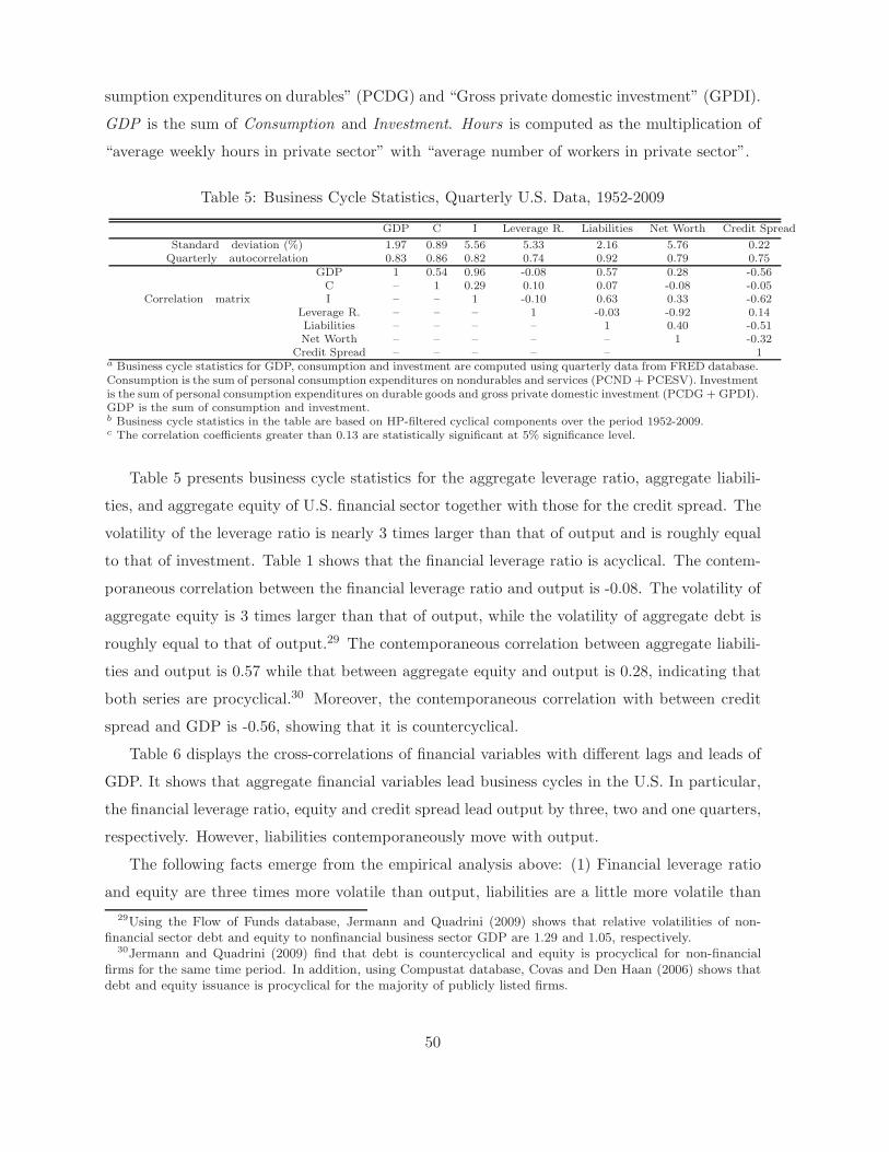
sumption expenditures on durables” (PCDG) and “Gross private domestic investment” (GPDI).

GDP is the sum of Consumption and Investment. Hours is computed as the multiplication of

“average weekly hours in private sector” with “average number of workers in private sector”.

Table 5: Business Cycle Statistics, Quarterly U.S. Data, 1952-2009

GDP C I Leverage R. Liabilities Net Worth Credit Spread

Standard deviation (%) 1.97 0.89 5.56 5.33 2.16 5.76 0.22Quarterly autocorrelation 0.83 0.86 0.82 0.74 0.92 0.79 0.75

GDP 1 0.54 0.96 -0.08 0.57 0.28 -0.56C – 1 0.29 0.10 0.07 -0.08 -0.05

Correlation matrix I – – 1 -0.10 0.63 0.33 -0.62Leverage R. – – – 1 -0.03 -0.92 0.14Liabilities – – – – 1 0.40 -0.51Net Worth – – – – – 1 -0.32

Credit Spread – – – – – 1a Business cycle statistics for GDP, consumption and investment are computed using quarterly data from FRED database.Consumption is the sum of personal consumption expenditures on nondurables and services (PCND + PCESV). Investmentis the sum of personal consumption expenditures on durable goods and gross private domestic investment (PCDG+ GPDI).GDP is the sum of consumption and investment.b Business cycle statistics in the table are based on HP-filtered cyclical components over the period 1952-2009.c The correlation coefficients greater than 0.13 are statistically significant at 5% significance level.

Table 5 presents business cycle statistics for the aggregate leverage ratio, aggregate liabili-

ties, and aggregate equity of U.S. financial sector together with those for the credit spread. The

volatility of the leverage ratio is nearly 3 times larger than that of output and is roughly equal

to that of investment. Table 1 shows that the financial leverage ratio is acyclical. The contem-

poraneous correlation between the financial leverage ratio and output is -0.08. The volatility of

aggregate equity is 3 times larger than that of output, while the volatility of aggregate debt is

roughly equal to that of output.29 The contemporaneous correlation between aggregate liabili-

ties and output is 0.57 while that between aggregate equity and output is 0.28, indicating that

both series are procyclical.30 Moreover, the contemporaneous correlation with between credit

spread and GDP is -0.56, showing that it is countercyclical.

Table 6 displays the cross-correlations of financial variables with different lags and leads of

GDP. It shows that aggregate financial variables lead business cycles in the U.S. In particular,

the financial leverage ratio, equity and credit spread lead output by three, two and one quarters,

respectively. However, liabilities contemporaneously move with output.

The following facts emerge from the empirical analysis above: (1) Financial leverage ratio

and equity are three times more volatile than output, liabilities are a little more volatile than

29Using the Flow of Funds database, Jermann and Quadrini (2009) shows that relative volatilities of non-financial sector debt and equity to nonfinancial business sector GDP are 1.29 and 1.05, respectively.

30Jermann and Quadrini (2009) find that debt is countercyclical and equity is procyclical for non-financialfirms for the same time period. In addition, using Compustat database, Covas and Den Haan (2006) shows thatdebt and equity issuance is procyclical for the majority of publicly listed firms.

50

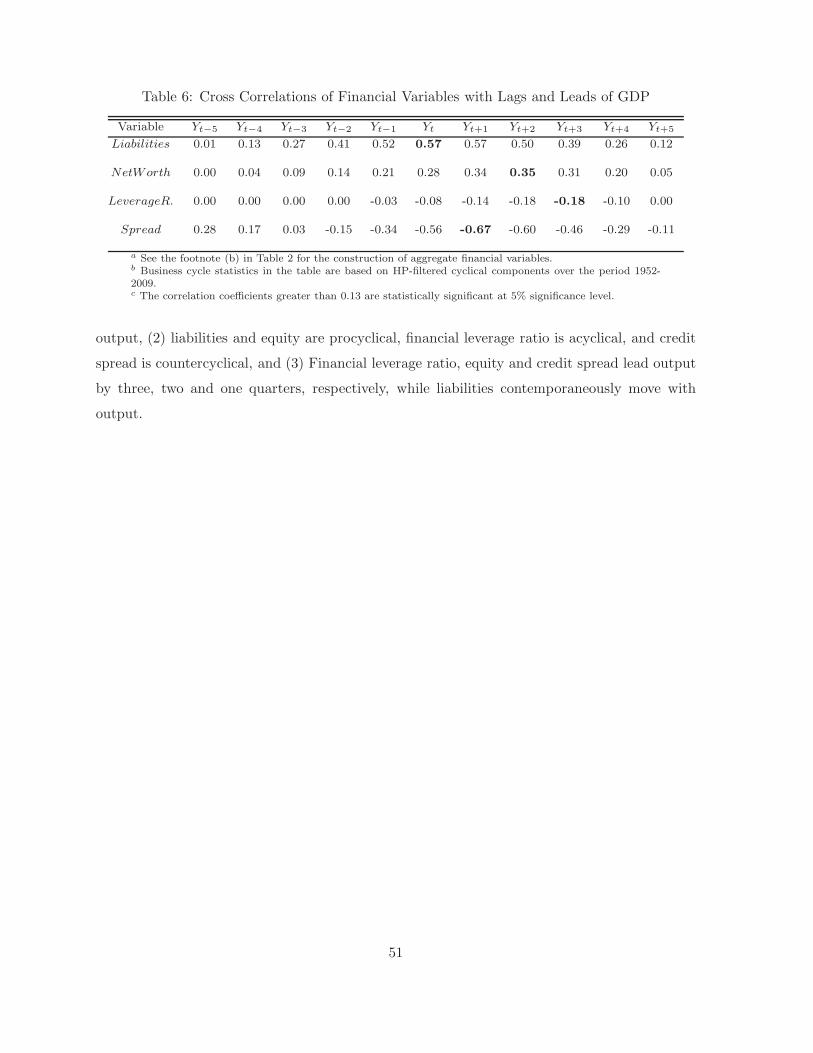
Table 6: Cross Correlations of Financial Variables with Lags and Leads of GDP

Variable Yt−5 Yt−4 Yt−3 Yt−2 Yt−1 Yt Yt+1 Yt+2 Yt+3 Yt+4 Yt+5

Liabilities 0.01 0.13 0.27 0.41 0.52 0.57 0.57 0.50 0.39 0.26 0.12

NetWorth 0.00 0.04 0.09 0.14 0.21 0.28 0.34 0.35 0.31 0.20 0.05

LeverageR. 0.00 0.00 0.00 0.00 -0.03 -0.08 -0.14 -0.18 -0.18 -0.10 0.00

Spread 0.28 0.17 0.03 -0.15 -0.34 -0.56 -0.67 -0.60 -0.46 -0.29 -0.11

a See the footnote (b) in Table 2 for the construction of aggregate financial variables.b Business cycle statistics in the table are based on HP-filtered cyclical components over the period 1952-2009.c The correlation coefficients greater than 0.13 are statistically significant at 5% significance level.

output, (2) liabilities and equity are procyclical, financial leverage ratio is acyclical, and credit

spread is countercyclical, and (3) Financial leverage ratio, equity and credit spread lead output

by three, two and one quarters, respectively, while liabilities contemporaneously move with

output.

51

Appendix E: Alternative Financial Shocks

This section presents alternative measures of financial shocks and the simulation results of the

benchmark models under these alternative measures. I label the benchmark model presented

in the text as Benchmark 1.

The first alternative measure for ωt series is constructed using the charge-off and delinquency

rates of all loans, the level of outstanding loans, and net worth of U.S. commercial banks from

the Federal Reserve Board:

ωt =(1 − Loanlossrates) ∗Outstandingloans

Networth(81)

Then I construct the log-deviation of ωt series by linearly detrending the log of these series

over the period 1987.Q1-2010.Q4. The ωt series can be interpreted as the level of recovery rates

of loans as a percentage of net worth. These recovery rates determine the level of credit con-

ditions in the economy since banks’ ability to extend loans to non-financial businesses depends

on their level of net worth, which can be seen from equation (20). Therefore, the innovations

to ωt are shocks to the recovery rates, hence to the level of financial conditions in the economy.

First, I estimate a VAR(1) for both TFP series and this alternative measure of ω. However,

the cross-terms in the VAR coefficient matrix are not statistically significant at 5% significance

level. Then I estimate two independent AR(1) processes for both series. The resulting persis-

tence of the ω series is ρω = 0.9690 and the standard deviation of the shock is σω = 0.003111.

The levels of zt and ωt series and the innovations to those series are plotted in Figure 11. I label

the model driven by both standard productivity shock and this alternative measure of financial

shock as Benchmark 2.

The second alternative measure for ωt series is constructed by calibrating the persistence,

ρω, and the standard deviation of the shock, σω, to match the persistence and the volatility

of net worth in the data. The resulting persistence is ρω = 0.55, and the resulting standard

deviation of the shock is σω = 0.04. I label the model driven by both standard productivity

shock and this alternative measure of financial shock as Benchmark 3.

Finally, the third alternative measure for ωt series is constructed as in the main text. How-

ever, this time I estimate a VAR(1) for both TFP and ω series instead of estimating two

independent AR(1) processes as follows:

52

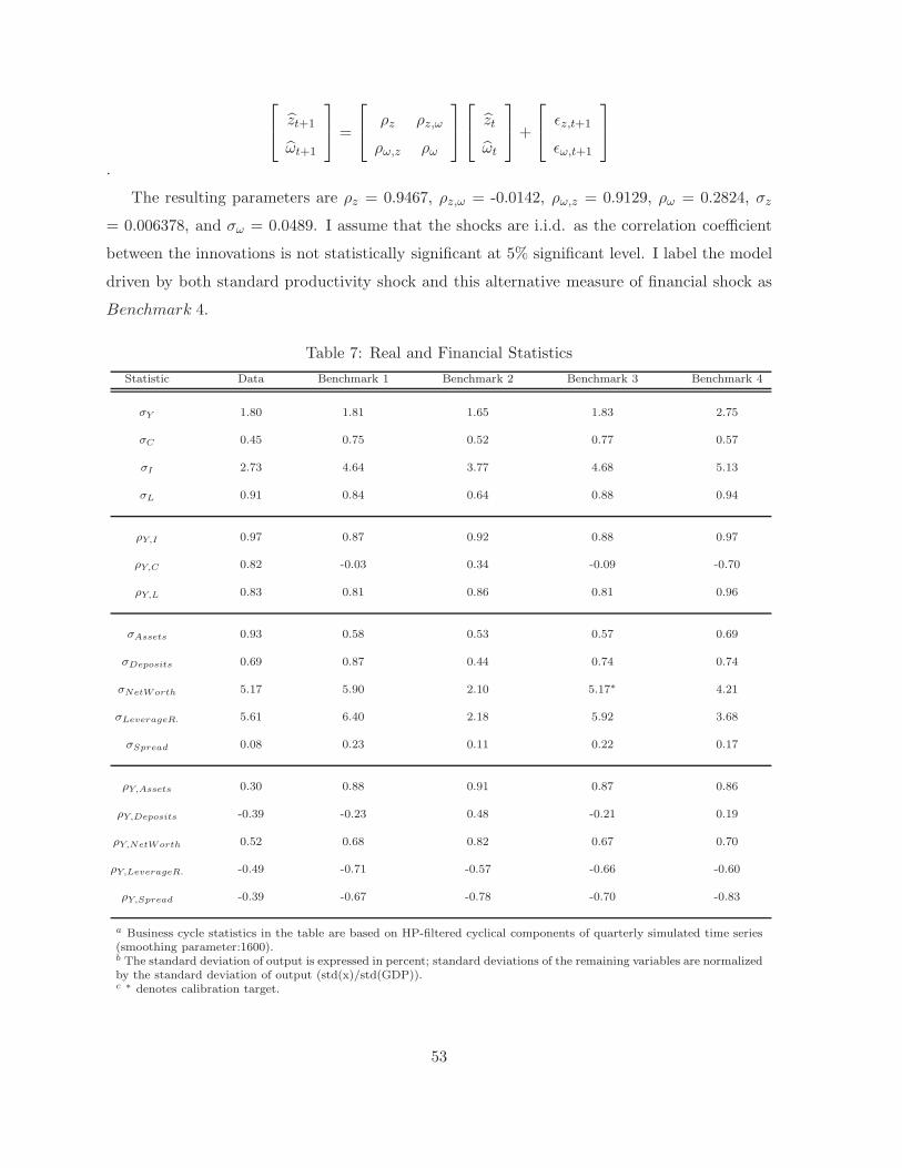
zt+1

ωt+1

=

ρz ρz,ω

ρω,z ρω

zt

ωt

+

ǫz,t+1

ǫω,t+1

.

The resulting parameters are ρz = 0.9467, ρz,ω = -0.0142, ρω,z = 0.9129, ρω = 0.2824, σz

= 0.006378, and σω = 0.0489. I assume that the shocks are i.i.d. as the correlation coefficient

between the innovations is not statistically significant at 5% significant level. I label the model

driven by both standard productivity shock and this alternative measure of financial shock as

Benchmark 4.

Table 7: Real and Financial Statistics

Statistic Data Benchmark 1 Benchmark 2 Benchmark 3 Benchmark 4

σY 1.80 1.81 1.65 1.83 2.75

σC 0.45 0.75 0.52 0.77 0.57

σI 2.73 4.64 3.77 4.68 5.13

σL 0.91 0.84 0.64 0.88 0.94

ρY,I 0.97 0.87 0.92 0.88 0.97

ρY,C 0.82 -0.03 0.34 -0.09 -0.70

ρY,L 0.83 0.81 0.86 0.81 0.96

σAssets 0.93 0.58 0.53 0.57 0.69

σDeposits 0.69 0.87 0.44 0.74 0.74

σNetWorth 5.17 5.90 2.10 5.17∗ 4.21

σLeverageR. 5.61 6.40 2.18 5.92 3.68

σSpread 0.08 0.23 0.11 0.22 0.17

ρY,Assets 0.30 0.88 0.91 0.87 0.86

ρY,Deposits -0.39 -0.23 0.48 -0.21 0.19

ρY,NetWorth 0.52 0.68 0.82 0.67 0.70

ρY,LeverageR. -0.49 -0.71 -0.57 -0.66 -0.60

ρY,Spread -0.39 -0.67 -0.78 -0.70 -0.83

a Business cycle statistics in the table are based on HP-filtered cyclical components of quarterly simulated time series(smoothing parameter:1600).b The standard deviation of output is expressed in percent; standard deviations of the remaining variables are normalizedby the standard deviation of output (std(x)/std(GDP)).c ∗ denotes calibration target.

53

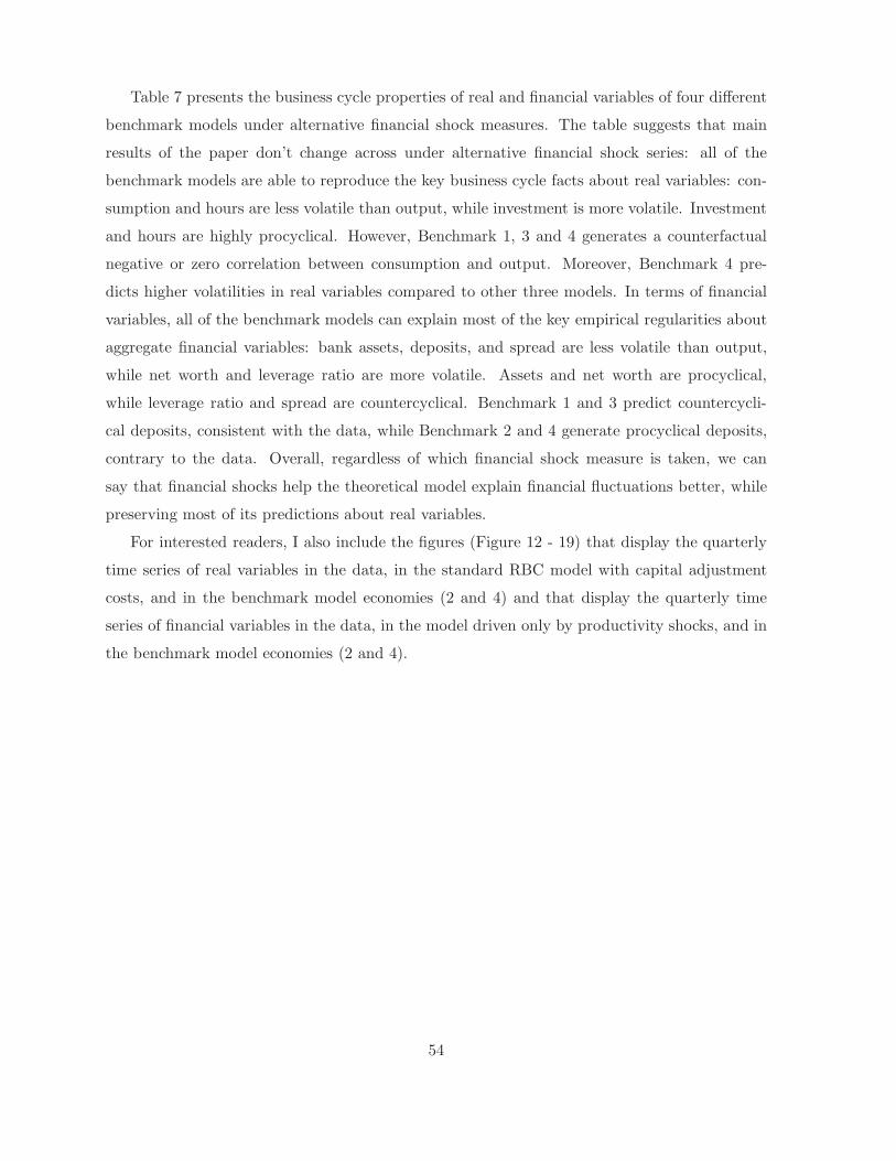
Table 7 presents the business cycle properties of real and financial variables of four different

benchmark models under alternative financial shock measures. The table suggests that main

results of the paper don’t change across under alternative financial shock series: all of the

benchmark models are able to reproduce the key business cycle facts about real variables: con-

sumption and hours are less volatile than output, while investment is more volatile. Investment

and hours are highly procyclical. However, Benchmark 1, 3 and 4 generates a counterfactual

negative or zero correlation between consumption and output. Moreover, Benchmark 4 pre-

dicts higher volatilities in real variables compared to other three models. In terms of financial

variables, all of the benchmark models can explain most of the key empirical regularities about

aggregate financial variables: bank assets, deposits, and spread are less volatile than output,

while net worth and leverage ratio are more volatile. Assets and net worth are procyclical,

while leverage ratio and spread are countercyclical. Benchmark 1 and 3 predict countercycli-

cal deposits, consistent with the data, while Benchmark 2 and 4 generate procyclical deposits,

contrary to the data. Overall, regardless of which financial shock measure is taken, we can

say that financial shocks help the theoretical model explain financial fluctuations better, while

preserving most of its predictions about real variables.

For interested readers, I also include the figures (Figure 12 - 19) that display the quarterly

time series of real variables in the data, in the standard RBC model with capital adjustment

costs, and in the benchmark model economies (2 and 4) and that display the quarterly time

series of financial variables in the data, in the model driven only by productivity shocks, and in

the benchmark model economies (2 and 4).

54

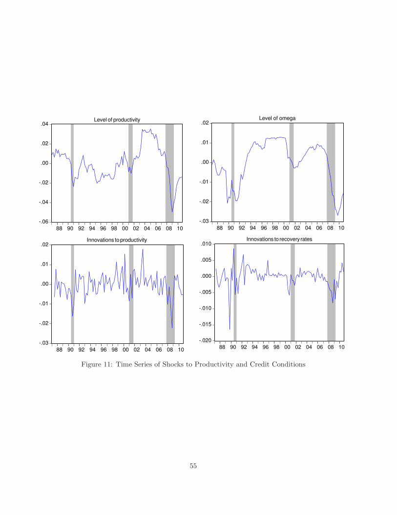
-.06

-.04

-.02

.00

.02

.04

88 90 92 94 96 98 00 02 04 06 08 10

Level of productivity

-.03

-.02

-.01

.00

.01

.02

88 90 92 94 96 98 00 02 04 06 08 10

Level of omega

-.03

-.02

-.01

.00

.01

.02

88 90 92 94 96 98 00 02 04 06 08 10

Innovations to productivity

-.020

-.015

-.010

-.005

.000

.005

.010

88 90 92 94 96 98 00 02 04 06 08 10

Innovations to recovery rates

Figure 11: Time Series of Shocks to Productivity and Credit Conditions

55

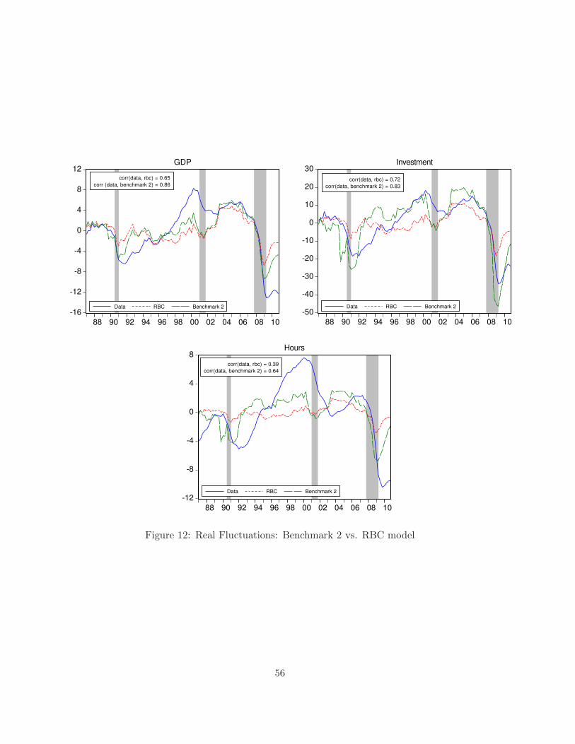
-16

-12

-8

-4

0

4

8

12

88 90 92 94 96 98 00 02 04 06 08 10


GDP


corr (data, benchmark 2) = 0.86

-50

-40

-30

-20

-10

0

10

20

30

88 90 92 94 96 98 00 02 04 06 08 10




Investment

-12

-8

-4

0

4

8

88 90 92 94 96 98 00 02 04 06 08 10




Hours

Figure 12: Real Fluctuations: Benchmark 2 vs. RBC model

56

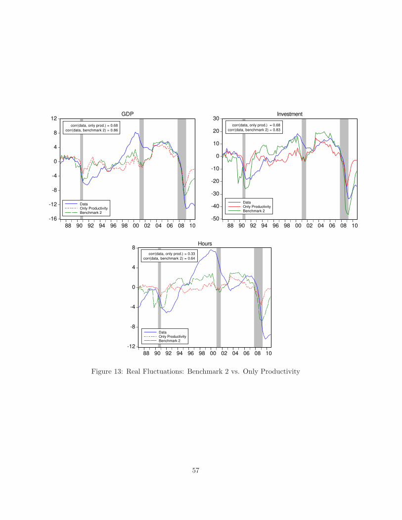
-16

-12

-8

-4

0

4

8

12

88 90 92 94 96 98 00 02 04 06 08 10




GDP

-50

-40

-30

-20

-10

0

10

20

30

88 90 92 94 96 98 00 02 04 06 08 10


Investment



-12

-8

-4

0

4

8

88 90 92 94 96 98 00 02 04 06 08 10


Hours



Figure 13: Real Fluctuations: Benchmark 2 vs. Only Productivity

57

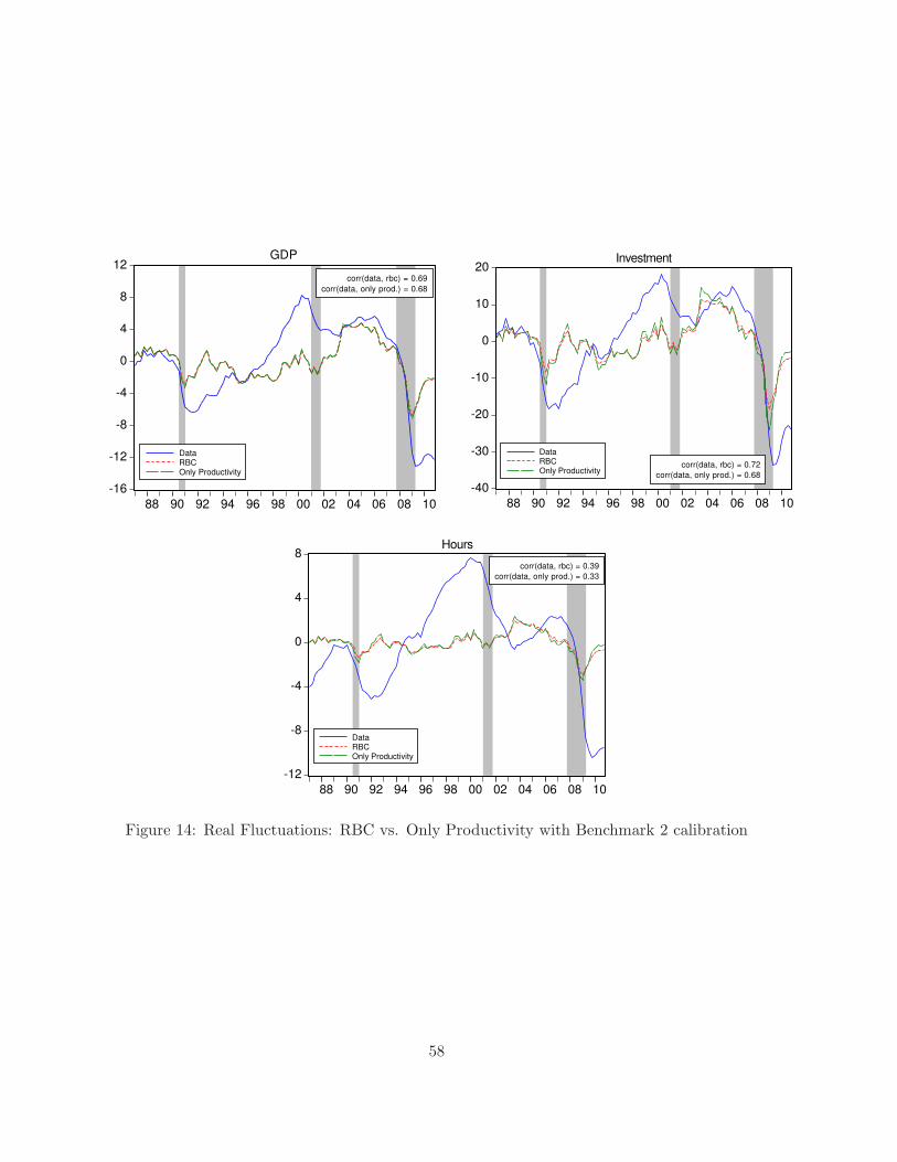
-16

-12

-8

-4

0

4

8

12

88 90 92 94 96 98 00 02 04 06 08 10


GDP



-40

-30

-20

-10

0

10

20

88 90 92 94 96 98 00 02 04 06 08 10


Investment



-12

-8

-4

0

4

8

88 90 92 94 96 98 00 02 04 06 08 10




Hours

Figure 14: Real Fluctuations: RBC vs. Only Productivity with Benchmark 2 calibration

58

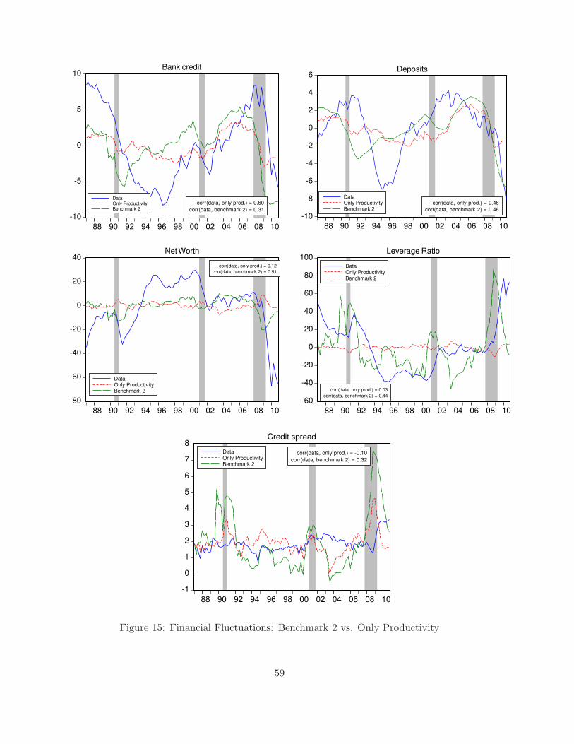
-10

-5

0

5

10

88 90 92 94 96 98 00 02 04 06 08 10


Bank credit



-10

-8

-6

-4

-2

0

2

4

6

88 90 92 94 96 98 00 02 04 06 08 10


Deposits



-80

-60

-40

-20

0

20

40

88 90 92 94 96 98 00 02 04 06 08 10




Net Worth

-60

-40

-20

0

20

40

60

80

100

88 90 92 94 96 98 00 02 04 06 08 10


Leverage Ratio



-1

0

1

2

3

4

5

6

7

8

88 90 92 94 96 98 00 02 04 06 08 10


Credit spread



Figure 15: Financial Fluctuations: Benchmark 2 vs. Only Productivity

59

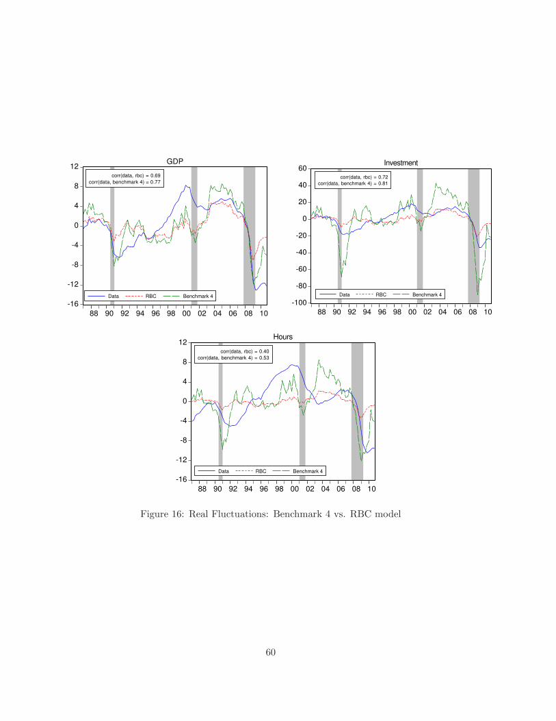
-16

-12

-8

-4

0

4

8

12

88 90 92 94 96 98 00 02 04 06 08 10


GDP



-100

-80

-60

-40

-20

0

20

40

60

88 90 92 94 96 98 00 02 04 06 08 10


Investment



-16

-12

-8

-4

0

4

8

12

88 90 92 94 96 98 00 02 04 06 08 10


Hours



Figure 16: Real Fluctuations: Benchmark 4 vs. RBC model

60

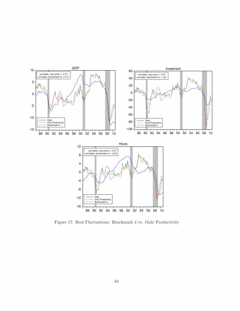
-15

-10

-5

0

5

10

88 90 92 94 96 98 00 02 04 06 08 10


GDP



-100

-80

-60

-40

-20

0

20

40

60

88 90 92 94 96 98 00 02 04 06 08 10


Investment



-16

-12

-8

-4

0

4

8

12

88 90 92 94 96 98 00 02 04 06 08 10


Hours



Figure 17: Real Fluctuations: Benchmark 4 vs. Only Productivity

61

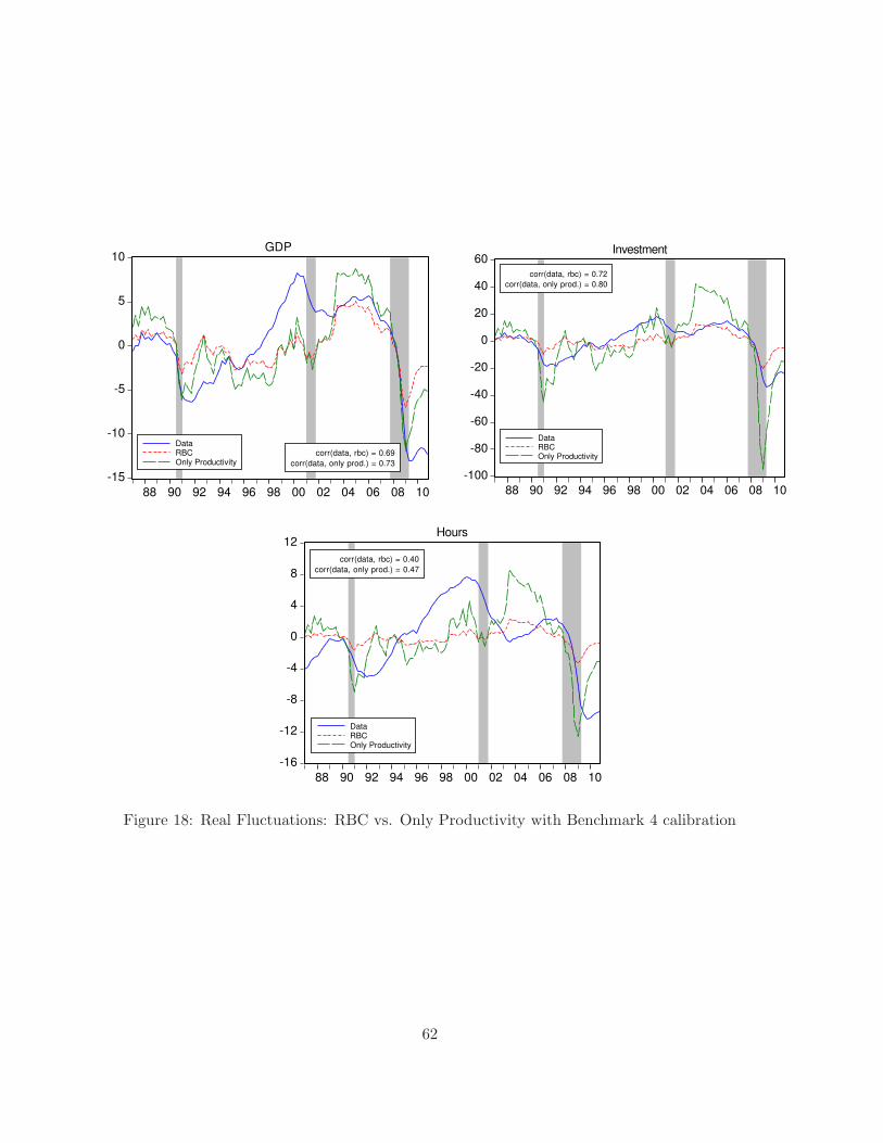
-15

-10

-5

0

5

10

88 90 92 94 96 98 00 02 04 06 08 10


GDP



-100

-80

-60

-40

-20

0

20

40

60

88 90 92 94 96 98 00 02 04 06 08 10


Investment



-16

-12

-8

-4

0

4

8

12

88 90 92 94 96 98 00 02 04 06 08 10


Hours



Figure 18: Real Fluctuations: RBC vs. Only Productivity with Benchmark 4 calibration

62

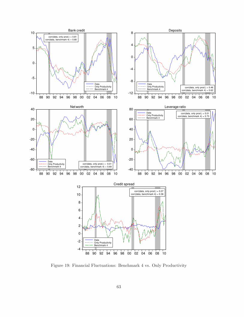
-10

-5

0

5

10

88 90 92 94 96 98 00 02 04 06 08 10


Bank credit



-12

-8

-4

0

4

8

88 90 92 94 96 98 00 02 04 06 08 10


Deposits



-80

-60

-40

-20

0

20

40

88 90 92 94 96 98 00 02 04 06 08 10


Net worth



-40

-20

0

20

40

60

80

88 90 92 94 96 98 00 02 04 06 08 10


Leverage ratio



-4

-2

0

2

4

6

8

10

12

88 90 92 94 96 98 00 02 04 06 08 10


Credit spread



Figure 19: Financial Fluctuations: Benchmark 4 vs. Only Productivity

63

Documents

Financial intermediaries, credit Shocks and business cycles · Munich Personal RePEc Archive Financial intermediaries, credit Shocks and business cycles Mimir, Yasin University of