ROLE OF INVESTMENT SHOCKS IN EXPLAINING BUSINESS CYCLES IN TURKEY

A THESIS SUBMITTED TO THE GRADUATE SCHOOL OF SOCIAL SCIENCES

OF MIDDLE EAST TECHNICAL UNIVERSITY

BY

CANAN YÜKSEL

IN PARTIAL FULFILLMENT OF THE REQUIREMENTS FOR

THE DEGREE OF MASTER OF SCIENCE IN

THE DEPARTMENT OF ECONOMICS

FEBRUARY 2012

iii

I hereby declare that all information in this document has been obtained and presented in accordance with academic rules and ethical conduct. I also declare that, as required by these rules and conduct, I have fully cited and referenced all material and results that are not original to this work. Name, Last Name: Canan Yüksel Signature:

iv

ABSTRACT

ROLE OF INVESTMENT SHOCKS IN EXPLAINING BUSİNESS CYCLES IN TURKEY

Yüksel, Canan

M. S., Department of Economics

Supervisor: Assoc. Prof. Dr. Ebru Voyvoda

February 2012, 87 pages

This thesis aims to understand the sources of business cycles observed in Turkish

economy. In particular the thesis investigates the role of investment shocks in

explaining fluctuations in output. For this purpose a small open economy DSGE

model is estimated on Turkish data for 2002-2011 period by Bayesian methods.

Variance decomposition analysis shows that permanent technology shock is the key

driving force of business cycles in Turkish economy and the role of investment

shock is less spelled.

Keywords: Open economy, Bayesian estimation, Business cycle

v

ÖZ

TÜRKİYE İŞ ÇEVRİMLERİNİN AÇIKLANMASINDA YATIRIM ŞOKLARININ ROLÜ

Yüksel, Canan

Yüksek Lisans, İktisat Bölümü

Tez Yöneticisi: Doç. Dr. Ebru Voyvoda

Şubat 2012, 87 sayfa

Bu tez, Türkiye ekonomisinde gözlenen iş çevrimlerinin kaynaklarını araştırmayı

amaçlamaktadır. Özellikle, üretimde gözlenen dalgalanmaları açıklamada yatırım

şoklarının rolü incelenmektedir. Bu amaçla Türkiye için 2002-2011 dönemi verileri

kullanılarak bir küçük açık ekonomi dinamik stokastik genel denge modeli, Bayesçil

yöntemlerle tahmin edilmektedir. Varyans ayrıştırma analizleri, kalıcı teknoloji

şoklarının Türkiye ekonomisinde gözlenen iş çevrimlerinin en önemli kaynağı

olduğunu, yatırım şoklarının rolünün ise daha sınırlı olduğunu göstermektedir.

Anahtar Kelimeler: Açık Ekonomi, Bayesçil Tahmin, İş Çevrimleri

vi

To My Family

vii

ACKNOWLEDGEMENTS

I would like to express my deepest gratitude to my thesis supervisor Assoc. Prof. Dr.

Ebru Voyvoda for her guidance and effort throughout this study. I would also like to

thank the examining committee members for their valuable comments and critiques.

I owe special thanks to The Scientific and Technological Research Council of

Turkey for the financial support they provided throughout my graduate study.

I would like to express genuine appreciation to Ali Rıza Yücel for his help, tolerance

and motivation. Without his invaluable company, this thesis could not be completed.

I also want to sincerely thank Harun Alp and Hande Küçük for their support and

helpful suggestions.

Finally, I am deeply indebted to my family, especially my mother Yasemin Yüksel,

for their unconditional love, care and encouragement throughout my entire life.

viii

TABLE OF CONTENTS

PLAGIARISM ........................................................................................................... iii

ABSTRACT .............................................................................................................. iv

ÖZ ............................................................................................................................... v

DEDICATION .......................................................................................................... vi

ACKNOWLEDGEMENTS ..................................................................................... vii

TABLE OF CONTENTS ........................................................................................ viii

LIST OF TABLES ..................................................................................................... x

LIST OF FIGURES ................................................................................................... xi

CHAPTER

1. INTRODUCTION ................................................................................................ 1

2. SYNOPSIS OF THE LITERATURE ON DSGE MODELING, BAYESIAN

ESTIMATION AND INVESTMENT SHOCKS .................................................. 6

2.1. Literature on DSGE Modeling ....................................................................... 6

2.2. Literature on Bayesian Estimation of DSGE Models .................................... 8

2.3. Literature on Investment Shocks .................................................................. 12

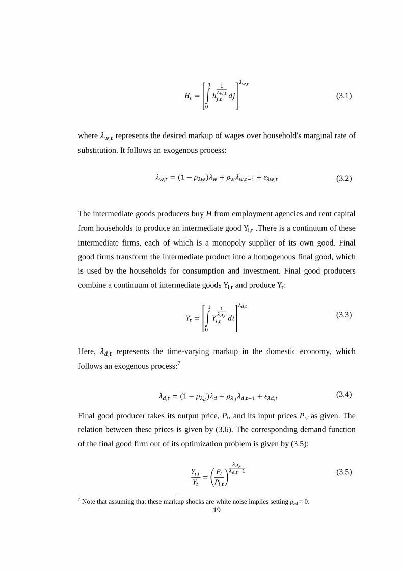
3. THE OPEN ECONOMY DSGE MODEL .......................................................... 17

3.1. Firms ............................................................................................................. 18

3.1.1. Domestic Firms ................................................................................ 18

3.1.2. Importing Firms ................................................................................. 22

3.1.3. Exporting firms .................................................................................. 24

3.2. Households ................................................................................................... 24

3.2.1. Wage Setting ..................................................................................... 30

3.3. The Government .......................................................................................... 30

3.4. The Central Bank ........................................................................................ 31

3.5. Foreign Economy ......................................................................................... 31

3.6. Market Clearing Conditions ......................................................................... 32

ix

3.7. Relative Prices .............................................................................................. 32

3.8. Model Solution ............................................................................................ 33

4. DATA AND METHOD ...................................................................................... 35

4.1. Data ............................................................................................................. 35

4.2. Method .......................................................................................................... 36

5. ESTIMATION ..................................................................................................... 40

5.1. Model Parameters ......................................................................................... 41

5.2. Model Fit ...................................................................................................... 45

5.3. Shocks and Business Cycles ........................................................................ 46

5.4. Model Dynamics and Shock Identification .................................................. 50

5.5. Discussion: The role of technology and investment shocks ........................ 51

6. CONCLUSION ................................................................................................... 56

REFERENCES ......................................................................................................... 58

APPENDICES ........................................................................................................... 64

A. The Log-linearized Model ............................................................................ 64

B. Tables and Graphs ........................................................................................ 66

x

LIST OF TABLES

TABLES

Table 5.1 Calibrated Parameters .............................................................................. 66

Table 5.2 Prior and Posterior Distributions .............................................................. 67

Table 5.3 Posterior variance decomposition in the model ........................................ 69

xi

LIST OF FIGURES

FIGURES

Figure 5.1a Prior and posterior distributions (Parameters) ...................................... 70

Figure 5.1b Prior and posterior distributions (Monetary policy parameters) ........... 71

Figure 5.1c Prior and posterior distributions (Shock processes parameter) ............. 71

Figure 5.2 Data and one-sided predicted values from the model ............................. 72

Figure 5.3 Historical decomposition of output ......................................................... 73

Figure 5.4 Impulse response to a unit-root technology shock .................................. 74

Figure 5.5 Impulse response to an investment shock ............................................... 74

Figure 5.6 Relative price of investment in Turkey ................................................... 75

Figure 5.7 Relative price of investment in U.S. ....................................................... 75

1

CHAPTER 1

INTRODUCTION

Explaining business cycles has been central in the public and academic debates for

long periods. Different methods have been used to understand fluctuations in

aggregate variables. On the one hand, the question is approached from the

perspective of general equilibrium models. Analyses based on general equilibrium

theory have claimed a central role for exogenous movements in total factor

productivity, i.e. neutral technology shocks (Kydland and Prescott, 1982, King and

Rebelo, 1999). On the other hand, the empirical approach to account for the business

cycle questioned the standard predictions of RBC model that productivity shocks are

the main source of business cycles. Moreover as discussed in Gali (1999), response

of hours to technology shocks is found to be hard to reconcile with data. This line of

research pointed at other disturbances such as labor supply shocks and oil prices

(Shapiro and Watson, 1988).

In the last two decades a new generation of micro-founded general equilibrium

models enriched with various nominal and real frictions gained popularity in many

fields of macroeconomic analysis, including business cycle analysis. The

developments on theory and estimation techniques of the so-called New Keynesian

models stimulated emergence of a new literature that examines business cycles from

a structural perspective. This approach involves estimation of Dynamic Stochastic

General Equilibrium (DSGE) models utilizing Bayesian techniques, focusing on the

historical and variance decomposition of main macroeconomic variables to explain

business cycles. Leading examples of this line of research are those examining

developed economies in closed economy settings (Smets and Wouters, 2003 and

Justiniano et al., 2010). However, besides a host of research in closed economy

2

models, open economy literature has not been far behind in utilizing Bayesian

techniques (Bergin, 2003, Dib, 2003, Del Negro et al., 2004, Adolfson et al., 2007).

This thesis aims to understand the main sources of output fluctuations in Turkish

economy in the last ten years within a general equilibrium framework. In particular

this thesis investigates the role of investment shocks in explaining business cycles,

whose contribution to macroeconomic fluctuations has been found to be significant

for developed economies (Justiniano et al., 2010, Smets and Wouters, 2007). Also

the importance of investment shock relative to other supply shocks such as stationary

and unit-root productivity shocks, which have been found to be important for

emerging market economies (Aguiar and Gopinath, 2007 and Alp and Elekdağ,

2011) is investigated. Understanding sources of business cycles is important for both

market participants and policy makers. Understanding the cyclical patterns is also

crucial for predicting and avoiding recessions and for policy design. For instance if

investment shock turns to be the most important driving force in the economy, a

policy advice to decrease output volatility would be decreasing the volatility of

investment shock. Since the investment shock is related to financing conditions than

taking measures to maintain financial stability may help to decrease volatilities of

both investment shock and economic activity. Therefore for policy design it is

important to know sources of business cycles. To this end, I develop a medium-scale

open economy DSGE model for Turkish economy and estimate it on quarterly data

using Bayesian estimation techniques. The model is buffeted by fourteen orthogonal

shocks, including permanent and stationary shocks to total factor productivity, an

investment shock, domestic and import mark-up shocks and a shock to labor supply.

Using data on fourteen macroeconomic variables including output, inflation, interest

rate, the real exchange rate, imports, exports and foreign economy variables for

2002:2-2011:3 period, key model parameters are estimated. The estimated model is

then used to address a number of key business cycle issues such as computing

variance decomposition of the observed variables and identifying the historical

evolution of underlying shocks that explain business cycles fluctuations.

3

The structural model used in this thesis generally follows the framework set by

Smets and Wouters (2003, 2007) and specifically extends the closed economy DSGE

model of Justiniano et al., (2010) by incorporating the open economy aspects. The

open economy features are in line with Adolfson et al. (2007). The theoretical model

also integrates a number of nominal and real frictions including sticky prices, sticky

wages, variable capital utilization, capital and investment adjustment costs and habit

persistence in consumption. There is incomplete exchange rate pass-through in the

import sector due to nominal price rigidities (i.e., local currency price stickiness)

whereas law of one price is assumed to hold in the export sector. Consistent with

small open economy perspective, foreign inflation, output and interest rate are

assumed to be exogenously given.

In particular, this thesis gives a special focus on the role of investment shocks in

understanding Turkish business cycles. Following the seminal work by Justiniano et

al. (2010), who find that a shock to the marginal efficiency of investment1 (MEI) is

the key driver of business cycles observed in U.S. economy, investment shocks

started to be one of the much debated driving forces in understanding

macroeconomic fluctuations. Prior to Greenwood et al. (1988), investment shocks

were considered as unlikely candidates to generate business cycles in a general

equilibrium environment. Justiniano et al. (2010) is the first study to attribute

investment shocks a key role in a DSGE setting. Among the studies examining

sources of business cycles (Smets and Wouters, 2003 and 2007; Adolfson et al.,

2007), permanent technology shocks and mark-up shocks have been the most

pronounced disturbances, whereas contributions of investment shocks were found to

be non-negligible, but less important. Especially for developing economies,

permanent technology shock was proposed to be the key driving force of

1 This shock affects the yield of a foregone unit of consumption in terms of future capital input. The literature often refers to this shock as investment specific technology shock, since the shock is equivalent to a productivity shock specific to the capital goods producing sector in a simple two-sector economy (Greenwood et al. 1997). Throughout the thesis I use the terms “MEI shock” and “investment shock” interchangeably.

4

macroeconomic fluctuations (Aguiar and Gopinath, 2007; Medina and Soto, 2007

and Alp and Elekdağ, 2011).

Role of various technology shocks including stationary, unit-root and investment

specific technology shock as a key source of business cycles is a debated issue in

macroeconomic analysis (Sims, 2011, Ravn and Simonelli, 2008). In general most of

the studies including Smets and Wouters (2003, 2007), Justiniano et al. (2010) show

that the three technology shocks combine to explain bulk of the cyclical variation in

output, where the stationary technology shock has the smallest contribution. Hence

the literature seems to agree on the overall importance of technology shocks relative

to non-technology shocks. However, the literature is far from a consensus on the

relative role of investment and permanent technology shocks. This thesis fits in this

lively part of the literature and tries to answer what role investment shocks play in

generating business cycles in Turkish economy.

The estimation results and variance decomposition analyses show that unit-root

technology, investment and exogenous spending shocks account for a large share of

output fluctuations in Turkish economy in the last ten years. In particular, the unit

root technology shock seems to be the most important of the technology shocks.

Such an outcome echoes the results of Aguiar and Gopinath (2007) which concludes

that this kind of trend shock is an important determinant of business cycle

fluctuations across emerging markets. There also seems to be an important

contribution by the exogenous spending shock. However in comparison to studies on

developed economies (e.g. Smets and Wouters, 2003, Adolfson et al. 2007), there

seems to be a limited role for the mark-up and stationary technology shocks. These

results are consistent with the findings of Alp and Elekdağ (2011), which is, to the

best of my knowledge, the only other study utilizing Bayesian methods for a small

open economy DSGE model tailored for Turkish economy.

The main contribution of this thesis is its provision of an analysis of Turkish

business cycles from the perspective of a fully articulated DSGE model. The Turkish

case often enforces an environment of working with short time series if the utilized

5

model does not account for structural break or policy switch since there is a policy

change and a set of structural reforms in post 2001 period, which should be taken

into account. Estimating the model by Bayesian methods enables one to take the

advantage of using prior information which is valuable while working with short

data samples. Moreover this thesis addresses a relevant question in the literature on

the relative importance of technology shocks in generating business cycles, by

incorporating stationary and unit root technology shocks and an investment specific

technology shock into the model.

The remainder of the thesis is organized as follows. Chapter 2 gives a brief review of

the related literature. In Chapter 3 the theoretical model is described. Chapter 4

contains a short description of the data and a review of Bayesian methods. In

Chapter 5, I first discuss the choice of parameters to calibrate, and the prior

distributions for the estimated parameters. Then, I report the estimation results and

compare the empirical properties of the estimated DSGE model with the actual data

to validate the model fit. In this Chapter, I also discuss the role of various shocks in

explaining Turkish business cycles. Finally, Chapter 6 concludes.

6

CHAPTER 2

SYNOPSIS OF THE LITERATURE ON DSGE MODELING, BAYESI AN ESTIMATION AND INVESTMENT SHOCKS

This chapter presents a review of the literature that is relevant for this thesis in three

parts. The first section provides a summary of the literature on DSGE modeling with

a special focus on the part of the literature which examines the sources of business

cycles. Section 2.2 reviews the empirical literature on the estimation of DSGE

models by the use of Bayesian techniques. This section discusses briefly the main

studies applying such methods and their findings2. Lastly, Section 2.3 summarizes

the literature investigating investment shocks and their findings. This section also

provides some inference on the meaning and propagation of shocks to marginal

efficiency of investment which is the main addressed disturbance in this thesis.

2.1. Literature on DSGE Modeling

This section provides an overview of the literature on theory of DSGE modeling, the

main reference framework for the analysis of economic fluctuations in modern

macroeconomic theory. In principle, DSGE models can help to identify sources of

fluctuations, answer questions about structural shifts, forecast and predict the effect

of policy changes, and perform counterfactual experiments. As a result of the ability

of DSGE models to address such policy-relevant questions, these models have also

been used by many policy-making institutions as a modeling framework.

Understanding the methodology of DSGE modeling requires a review of the

transition from traditional quantitative macroeconomic models towards the so-called

New Keynesian (NK) framework. The traditional macro models consist of a set of

2 A detailed description of the method is presented in Chapter 4.

7

ad-hoc equations mimicking the behavior of key aggregate macroeconomic variables

instead of an optimization-based approach. Failure of these models to predict the

stagflation observed during the 1970s led to weakening of their popularity. This

breakdown in the performance of these macroeconometric models together with the

rational expectations revolution inspired by the Lucas critique gave way to the

emergence of real business cycle (RBC) theory introduced by Kydland and Prescott

(1982)3. For the first time, this paper proposed a small and coherent dynamic model

of the economy, built from first principles with optimizing agents, rational

expectations, and market clearing, that could match stylized facts in the data at a

remarkable degree. The RBC models consider business cycles as efficient responses

of a frictionless economy to exogenous movements in total factor productivity.

Although these models were criticized on many aspects (such as assumption of

frictionless, perfectly competitive markets, inability to match data on movement of

hours and wage), methods of RBC approach have still been employed and the

general structure of the RBC models with its “optimizing agents in a general

equilibrium setting” is preserved in DSGE models.

Emergence of the New Keynesian (NK) paradigm is considered as an attempt to

provide micro-foundations for resuscitating basic Keynesian concepts such as market

imperfections, the inefficiency of aggregate fluctuations and rationale for policy

making, as opposed to the RBC approach. Hence most of the work in NK literature,

including Calvo (1983), Bernanke et al. (1999), Clarida et al. (1999), aimed to

provide microfoundations such as nominal and real rigidities, financial market

imperfections, and to incorporate these into general equilibrium models. DSGE

models were developed by feeding of these mechanisms into the stochastic

neoclassical growth model of Kydland and Prescott (1982).

The literature on open economy DSGE models was engendered by the contribution

of Obstfeld and Rogoff (1995). Closed economy setting in the early works of DSGE

models had problems in matching some facts in the data. To overcome such

3 King and Rebelo (1999) provides a detailed review of RBC models.

8

problems, open economy models incorporated the possibility that international trade

in final goods and financial assets affects the evolution of the domestic economy

giving rise to richer dynamics. Prominent studies on this line are Gali and Monacelli

(2002) and Monacelli (2003). The former develops a small open economy model

(SOEM) incorporating many of the microfoundations appearing in the closed

economy NK framework, summarized in Woodford (2003). Monacelli (2003) on the

other hand allows for local currency pricing of traded goods and presents a

mechanism for limited pass-through of exchange rate movements to consumer

prices. The SOEM in Adolfson et al. (2007) incorporates all the features of closed

economy models, summarized in Christiano et al. (2005), and adds up some open

economy features such as consumption and investment of foreign goods, saving in

foreign bonds and incomplete exchange rate pass-through to both import and export

prices. Their work provides an elegant example that nests most of the developments

in the literature.

To sum up, over the past 25 years DSGE models, with their coherent frameworks,

have become increasingly popular in both academia and in non-academic circles.

Policy makers have become increasingly interested in usefulness of DSGE models

for policy analysis and forecasting. This type of modeling approach seems to

continue to be the reference framework for macroeconomic analysis.

2.2. Literature on Bayesian estimation of DSGE models4

Regarding the application of Bayesian techniques, this thesis is related to the large

literature using estimated micro-founded models to understand the main sources of

business cycle fluctuations (Smets and Wouters, 2003, Adolfson et al., 2007,

Justiniano et al., 2010). With the explosion of research using Bayesian methods, the

formal estimation of DSGE models has become one of the cornerstones of modern

macroeconomics. This section presents the evolution of the literature towards use of

4This section is based on An and Schorfheide (2006), Lubik and Schorfheide (2007) and Fernández-Villaverde (2009), as main references that present detailed reviews of Bayesian methods in macroeconomic analyses.

9

Bayesian techniques in DSGE analysis. Moreover, the findings of leading examples

of the Bayesian DSGE literature, related to business cycle analysis, are presented in

this subsection.

Although DSGE models provide a complete multivariate stochastic process

representation for the data, for a long time they were in many cases rejected against

less restrictive specifications such as vector autoregressions (VAR). That was

because the quantitative evaluation of DSGE models was conducted without formal

statistical methods and the models constituted a framework that is more restrictive

than VARs. Subsequently with the improvement of the structural models and the

amendment of some misspecified restrictions, more traditional econometric

techniques have become applicable such as generalized method of moments (GMM)

estimation of equilibrium relationships, minimum distance estimation based on the

discrepancy among VAR and DSGE model impulse response functions, (Christiano

et al., 2005). However, as discussed in An and Schorfheide (2007), the econometric

analysis of DSGE models has to cope with several challenges, including potential

model misspecification and identification problems5. In recent years, to address these

challenges, methods that are built around a likelihood function derived from the

model, such as a Bayesian framework, have been developed for empirical work with

DSGE models.

Bayesian estimation of DSGE models has three main advantages. First, instead of an

estimation based on equilibrium relationships, the Bayesian analysis is system-based

and it fits the solved DSGE model to a vector of aggregate time series. Second, the

estimation is based on the likelihood function generated by the DSGE model itself

rather than, for instance, the discrepancy between DSGE model responses and VAR

impulse responses. Third, the use of priors enables the researcher to include

additional information which helps to sharpen inference and provides a useful device

5 DSGE model misspecification can take many forms including omitted non-linearities, misspecified structural relationships, or misspecification due to wrongly-specified exogenous processes. The identification problems may arise due to omitting a relevant observation or from a case where probability model implies different values of parameters lead to same joint distribution for the observable variables (Lubik and Schorfheide, 2007).

10

for incorporating micro-level information in the estimation of aggregate time series

model. Prior distributions can be used to incorporate additional information into the

parameter estimation and to re-weight the likelihood function so that the peak

appears in a region of the parameter space that is consistent with extraneous

information. This helps especially when data do not include information that’s

needed for identification of parameters. For example, estimates of the discount factor

should be consistent with the average magnitude of real interest rates, even if the

estimation sample does not include observations on interest rates. Moreover, use of

prior information in Bayesian analysis provides a further advantage to cope with

identification problems. In such a case even a weakly informative prior helps to

update the likelihood function in directions of the parameter space in which it is not

flat. This way the prior can introduce curvature into the posterior density surface that

facilitates numerical maximization. Hence, Bayesian analysis provides a powerful

framework for DSGE model estimation and inference.

The literature on likelihood-based Bayesian estimation of DSGE models is generally

based on the studies by Landon-Lane (1998), DeJong et al. (2000), Schorfheide

(2000) and Otrok (2001). The abovementioned superiorities of Bayesian estimation

methods and the improvement in computational tools stimulated the use of Bayesian

techniques in formal estimation and evaluation of DSGE models. A prominent

example towards such a target is Smets and Wouters (2003). This paper estimates a

medium-scale closed economy DSGE model for Euro area for 1980:2-1999:4 period

and finds that the productivity and wage mark-up shocks are the main driving forces

of output in medium to long run. Smets and Wouters (2003) also concludes that

investment specific technology shock accounts for a significant, but much less

important fraction of output developments at business cycle frequency. In a similar

model estimated for U.S. economy, covering the period 1966:1-2004:4, Smets and

Wouters (2007) finds that the identified sources of business cycle fluctuations and

the effects of various shocks are similar to their findings for Euro Area. In another

study for U.S. economy using 1954:3-2004:4 data, Justiniano et al. (2010) proposes

that shocks to marginal efficiency of investment (MEI) is the main source of

11

business cycles and this shock can explain more than half of the volatility in output.

Justiniano et al. (2011) arrives at a similar conclusion based on estimating a

medium-scale DSGE model for the U.S. economy by using the additional

information in relative investment prices. This paper introduces two different types

of investment shocks: first is the MEI shock which hits the capital good producer

sector affecting the production of installed capital from investment goods and is

related to factors other than price movements. The second is the investment specific

technology (IST) shock that hits the investment good producing sector. This shock

affects the transformation of consumption into investment goods and is identified

with the relative price of investment. In this setting, Justiniano et al. (2011)

concludes that the MEI shock remains to be the main source of business cycles while

the role of IST shocks is negligible. On the other hand, Christiano et al. (2010)

suggests a negligible role for MEI shocks and proposes a different source of

variation (the risk shock) that governs the investment returns. Estimating a closed

economy model, enriched with financial frictions and a banking sector, they

conclude that the main source of fluctuations in both U.S. and Euro area is the risk

shock.

Besides such closed economy studies, the question of “what is the main source of

macroeconomic fluctuations” is also discussed in the open economy context by

using Bayesian estimation techniques. For example, Justiniano and Preston (2004)

considers the situations of imperfect exchange rate pass-through. Similarly Lubik

and Schorfheide (2007) examines whether the central banks respond to exchange

rates in open economies such as Australia and Canada. The distinguishing study by

Adolfson et al. (2007) analyzes an open economy model that includes variable

capital utilization as well as numerous real and nominal frictions and examines

sources of business cycles in Euro Area in 1970:1-2002:4 period. According to their

results, technology and mark-up shocks (especially in the Philips curves for import

and export goods) appear to be of importance.

12

For Turkey, Alp and Elekdağ (2011) estimates a SOEM with financial accelerator

channel. They find that the unit-root and investment-specific technology shocks are

the two prominent supply shocks in explaining output fluctuations, whereas mark-up

and stationary technology shocks play a limited role as a source of economic

fluctuations.

2.3. Literature on Investment Shocks

This section gives a brief review of the literature that discusses the role of shocks to

marginal efficiency of investment (MEI) in macroeconomic fluctuations.

The MEI shock is either introduced as a shock to investment cost function as shown

in (2.1) (Smets and Wouters, 2003) or as a source of exogenous variation in the

efficiency with which the final good is transformed into physical capital as shown in

(2.2) (JPT 2010 and 2011). In the latter specification, MEI shock affects the yield of

a foregone unit of consumption in terms of next period’s capital input.

����� = �1 − ����� + ���1 − ������/������ (2.1)

����� = �1 − ����� + �����1 − ����/������ (2.2)

Until late 1990’s, investment shocks have been considered as unlikely candidates to

generate business cycles in standard neoclassical environments, because they cannot

generate the co-movement of key macroeconomic variables. Consider a case where a

positive shock to the MEI hits the economy leading to an increase in the rate of

return on existing capital. This leads households to save more, consume less, but also

to work harder. Since capital remains fixed in the short run, labor productivity and

real wage are expected to fall. Hence a positive MEI shock creates a situation where

working hours and output rise but consumption moves in opposite direction and

falls, which is not a recognizable business cycle fact. This premise can be understood

better from the efficiency condition which has to hold in a frictionless closed

economy:

13

( ) ( )LMPLLCMRS ≡, (2.3)

Note that marginal rate of substitution (MRS) between consumption and hours

depends positively on its arguments, whereas marginal product of labor (MPL) is

decreasing in hours worked. As Barro and King (1984) points out, any shock that

rises hours, without shifting the marginal product of labor, leads the right hand side

(RHS) of (2.3) to fall. For condition (2.3) to hold at the new equilibrium,

consumption should be falling so that the left hand side (LHS) of (2.3) falls down as

well. Indeed, this is the way how investment shock transmits into the economy and

creates an opposite movement in consumption and hours. Therefore the literature did

not give much credit to MEI shocks as a driving force of business cycles.

Greenwood et al. (1988) was the first to suggest investment shocks as a viable

alternative to neutral technology shocks in a general equilibrium framework. This

paper investigated the role of investment-specific technological change in generating

postwar U.S. growth. In their model, there are two types of capital one of whose

evolution is subject to a specific technology change. This paper concluded that IST

change accounts for the major part of growth in the post-war U.S. In a later study

Greenwood et al. (2000) strengthens the previous conclusion by showing that this

form of technological change can explain about 30% of postwar U.S. output

fluctuations. In another study examining U.S. economy by a structural VAR

analysis, Fisher (2006) shows that investment shocks have a prominent role in

business cycles and changes in the relative price of investment accounts for a large

part of the fluctuations in output and hours. Moreover Canova et al. (2006) finds

similar results. These studies were motivated by the observed fall in price of

investment relative to consumption in the post-war U.S. and assume that the

production of capital goods becomes increasingly efficient with the passage of time.

They identified investment disturbances with the trend fall in relative price of

investment.

14

With the increasing feasibility and popularity of Bayesian methods in

macroeconomic analysis, the importance of investment shocks for business cycles is

also analyzed by Bayesian estimation of DSGE models. Justiniano, Primiceri and

Tambalotti (JPT) (2010, 2011) address this issue in a New Neoclassical Synthesis

model of the US economy6. They treat the investment shock as an unobservable

process and identify it through its dynamic effects on the variables included in the

estimation. They find that a MEI shock, which determines the efficiency of newly

produced investment goods, is the key driver of U.S. business cycles explaining

more than 50 percent of the observed volatility in output. On contrary to the

aforementioned problems related to MEI shocks in generating co-movement of key

macroeconomic series, this paper shows that consumption, hours and output move in

the same direction as a response to MEI shock. This finding owes to the newly

introduced channels, which were absent in a standard neoclassical model. JPT (2010)

highlights that the existence of nominal and real rigidities along with endogenous

capital utilization and internal habit formation (in consumption) operate to make the

transmission of investment shocks more conformable with the typical pattern of

business cycles. These three features of the model break the equilibrium condition

(2.3) and help generating movement of the main macroeconomic variables in same

direction. First, internal habit formation limits the adjustments in consumption in

response to a MEI shock and consumption becomes less likely to fall when a

positive shock hits the economy. On the other hand, endogenous capital utilization

works through MPL. In response to a positive MEI shock, utilization of existing

capital increases as new investment becomes more efficient. Higher capital

utilization, in turn, implies an increase in the marginal product of labor affecting the

RHS of (2.3). In addition, price and wage stickiness create a wedge between MPL

and MRS such that equilibrium condition becomes:

( ) ( ) ( )LMPLLCMRSL ≡,ω (2.4)

6 The question and the main techniques applied in this thesis are largely based upon JPT (2010).

15

In (2.4), ω(L) can be treated as the sum of price and wage mark-up. When this

wedge is countercyclical, i.e. ω(L) is decreasing in hours, one can observe a rise in

both consumption and hours in response to a positive MEI shock since the required

fall in LHS now takes place through ω(L). JPT (2010) points that the existence of

price and wage rigidities is the main channel that leads MEI shock to be the most

important driving force of business cycles and concludes that the role of MEI shocks

becomes negligible in a flexible price and wage economy.

JPT (2010) is the first to find such a high explanatory power of MEI shock in an

estimated DSGE model. In a quite similar model Smets and Wouters (2007) finds a

smaller contribution of MEI shocks to volatility of output. JPT (2010) concludes that

the main reason for this divergence of the results of the two related papers is the

difference in definitions of consumption and investment variables.

The ultimate origin of MEI shocks is another debated issue in this part of the

literature. JPT (2011) points out that MEI shock can be treated as a proxy for the

effectiveness of financial intermediation in channelling household savings into

productive capital since the transformation of investment goods into productive

capital is closely related to financial conditions and access to credit plays an

important role in this process. For instance JPT (2011) shows that the estimated

series of MEI shock displays a strong negative relation with a spread measure (i.e.

the spread between high-yield and AAA corporate bonds). Although absent in JPT

(2010, 2011) and, also in this thesis, introducing financial accelerator mechanism

could motivate a similar propagation endogenously. In such a model, part of the new

capital would be destroyed because of the agency cost (��) associated with

monitoring costs and would constitute a drain on the capital formation process:

����� = �1 − ����� + ���1 − ��� (2.5)

Equation (2.5) is quite comparable to (2.2). As JPT (2011) points out, this

mechanism would be similar to a MEI shock in the sense that it also introduces a

randomness and interruption in the capital formation process.

16

To capture the link between MEI shock and financial sector, JPT (2011) presents an

additional version of their baseline model which is estimated by adding spread data

among observables. In that version MEI shocks still explain an important, but lower,

part (around 40 percent) of output fluctuations compared to the baseline model. On

the other hand, in a recent paper Chrisitano et al. (2010) investigates the sources of

business cycles in a DSGE model enriched with financial factors and introduces a

shock to risk, which emanates from the financial sector. They show that this risk

shock turns out to be the most important source of fluctuations and it crowds out

some of the role of the MEI shocks. This fact also hints a close relation between the

MEI shocks and financial conditions in the economy.

17

CHAPTER 3

THE OPEN ECONOMY DSGE MODEL

This chapter gives an overview of the model economy and presents the key

equations in the theoretical model. It is a small open economy DSGE model quite

similar to the one developed in Adolfson, Laséen, Linde and Villani (ALLV) (2007)

and shares its basic closed economy features with many recent new Keynesian

models, including the models of Christiano et al. (2005), Smets and Wouters (2003)

and Justiniano et al. (2010). The model incorporates several open economy features,

as well as a number of nominal and real frictions such as sticky prices, sticky wages,

variable capital utilization, capital and investment adjustment costs and internal habit

persistence that are proved to be important for the empirical fit of the models. The

model used in this thesis has also similarities with that of Alp and Elekdağ (2011)

except the financial accelerator mechanism in the latter. On the contrary, there is no

explicit role for financial intermediation in this thesis.

The model economy is populated by households, domestic firms, importing and

exporting firms, a government, a central bank, and an exogenous foreign economy.

The households consume a basket of domestically produced goods and imported

goods, which are supplied by importing firms. The model allows the imported goods

to enter the aggregate investment as well as aggregate consumption, considering the

significantly high share of imports in total investment in Turkey. Households can

save in domestic and/or foreign bonds. The choice between domestic and foreign

bonds balances into an arbitrage condition (i.e., an uncovered interest rate parity

condition) which is a key equation of this model. Households rent capital to the

domestic firms and decide how much to invest in their stock of capital given the

investment adjustment costs. The model introduces wage stickiness through an

indexation variant of the Calvo (1983) model.

18

Domestic production is exposed to a stationary and a stochastic unit root technology

growth. The domestic and importing firms produce differentiated goods and set

prices a la Calvo model. By including nominal rigidities in the importing sector, the

model allows for short-run incomplete exchange rate pass-through to import prices.

On the other hand, following Gertler et al. (2007), I assume that foreign demand for

the home tradable good (i.e. the demand for home country exports) is exogenously

given and the law of one price holds for the exporting sector.

Monetary policy is approximated with a Taylor-type interest rate rule whereas

government spending is assumed to be an exogenous AR(1) process. Adopting a

small open economy perspective, the foreign economy is taken to be exogenous.

Accordingly the foreign inflation, output and interest rate are assumed to be given by

exogenous AR(1) processes. The following section provides the optimization

problems of the different firms and the households, and describes the behavior of the

central bank and the government.

3.1. Firms

There are three categories of firms operating in this economy: domestic, importing

and exporting firms. The intermediate domestic firms produce a differentiated good,

using capital and labor inputs, which they sell to a final good producer who

transforms a continuum of these intermediate goods into a homogenous final good.

The importing firms, in turn, buy a homogenous good in the world market, and sell it

to the domestic households after transforming into a differentiated import good. The

exporting firms buy the domestic final good and sell it in the world market.

3.1.1. Domestic Firms

There are three types of domestic firms. First type is the employment agencies. They

operate competitively and combine the specialized labor of each household j into a

homogenous labor input H and sell to the intermediate goods producers:

19

�� = ��ℎ�,����,��

!"#��,�

(3.1)

where $%,� represents the desired markup of wages over household's marginal rate of

substitution. It follows an exogenous process:

$%,� = �1 − &�%�$% + &%$%,��� + '�%,� (3.2)

The intermediate goods producers buy H from employment agencies and rent capital

from households to produce an intermediate good Y),* .There is a continuum of these

intermediate firms, each of which is a monopoly supplier of its own good. Final

good firms transform the intermediate product into a homogenous final good, which

is used by the households for consumption and investment. Final good producers

combine a continuum of intermediate goods Y),* and produce Y*: +� = ��+,,���-,�

�

!.#�-,�

(3.3)

Here, $/,� represents the time-varying markup in the domestic economy, which

follows an exogenous process:7

$/,� = �1 − &�-�$/ + &�-$/,��� + '�/,� (3.4)

Final good producer takes its output price, Pt, and its input prices Pi,t as given. The

relation between these prices is given by (3.6). The corresponding demand function

of the final good firm out of its optimization problem is given by (3.5):

+,,�+� = 0 1�1,,�2�-,��-,���

(3.5)

7 Note that assuming that these markup shocks are white noise implies setting ρλd = 0.

20

1� = ��1,,� ����-,��

!.#���-,�

(3.6)

The production function of the intermediate firm i is given by:

+,,� = 3��,,�4 �5��,,����4 − 5�6 (3.7)

where Ki,t and Hi,t are the capital services and labor inputs used by firm i,

respectively. 6 is a fixed cost of production. This parameter is chosen such that zero

profit condition holds at steady state. Moreover it is assumed to grow at the same

rate as output do in steady state. Otherwise, the fixed cost would become irrelevant

and profits would tend to be systematically positive as a result of monopoly power of

the firms. 3� is a covariance stationary technology shock and 5� is a permanent

technology shock. Level of permanent technology is non-stationary and its growth

rate, (µz,t = log (zt / zt-1) follows an AR(1) process:

μ8,� = �1 − &9:�μ8 + &9:μ8,��� + '8,� (3.8)

The stationary shock has the following representation:

3� = &<3��� + '<,� (3.9)

To ease notation, throughout the thesis, a variable with a hat denotes the log-

deviations from steady-state values.

Given Pi,t, the intermediate firm that is constrained to produce Yi,t faces the following

cost minimization problem:

21

=.>?@��,,� + A�B�,,� + $�1,,�C+,,� − 3��,,�4 �5��,,����4 + 5�6DE (3.9)

Rk is the gross nominal rental rate per unit of capital services and Wt is the nominal

wage rate per unit of labor Hi,t..

The first order conditions for the optimization (3.10) with respect to H and K are:

@� = �1 − F�$�1,,�3�5���4��,,����,,��4 (3.11)

A�B = F$�1,,�3�5���4��,,����,,����4 (3.12)

The price rigidity is introduced a la Calvo (1983). The intermediate firms are

allowed to change their price only when they receive a random price change signal.

Every period there is a random probability G/ that intermediate firms cannot readjust

price optimally but choose according to the indexation rule:

1��� = 1� H�I- �H���J ���I- (3.13)

where H� is the gross inflation rate H� = �1�/P���� and HJ is the inflation target.

With probability �1 − G/�, the firm can choose its price optimally by maximizing the

present discounted value of future profits as follows :

L� MN�G/O�P�P R1ST%,� UVH��B��I- �H��BJ ���I-P

BW�X+,,��PY

PW −Z[,,��P\+,,��P + 5��P6]^_

(3.14)

ν is the household's marginal utility of income and existence of that in the price

setting makes profits conditional on utility. Pnew is the re-optimized price and MC is

the firm’s nominal marginal cost. Consequently, the average price in period t is:

1� = `G/\1��� H���I- �H�J���I-] ����-,� + �1 − G/�\1ST%,�] ����-,�a���-,� (3.15)

22

Log-linearizing this condition gives the domestic price Philips curve:

Hb� − Hb�J = O1 + Oc/ �L�Hb��� − &dHb�J�+ c/1 + Oc/ �Hb��� − Hb�J� − c/O�1 − &d�1 + Oc/ Hb�J+ �1 − G/��1 − OG/�G/�1 + Oc/� \=ef � + $g/,�]

(3.16)

3.1.2. Importing Firms

The importing firms buy a homogenous good in the world market at price P* and

transform it into a differentiated good under “brand naming”. There is a continuum

of importing firms which sell their differentiated goods to the households. The

model allows for incomplete exchange rate pass-through to import prices by the

assumption of local currency price stickiness. Price setting process of importing

firms is similar to that of intermediate goods producers. Each importing firm can re-

optimize its price in any period with a random probability (1−ξm). Importing firms

cannot reset their price optimally with probability ξm but choose according to the

indexation rule:

1���h = 1�h�H�h�Ii �H���J ���Ii (3.17)

H�h = �1�h/1���h � is the import price inflation. The importing firm i who sells Mi

amount of imported goods, maximizes the following discounted profits:

L� MN�GhO�Pν��PC1ST%,�h Z,,��P�H�h…H��P��h �Ii �H���J …H��PJ ���Ii

YPW

− ���P1��P∗ \Z,,��P + 5��P6h]D_ (3.18)

Φm is the fixed cost of the imported good firm and it is introduced to make import

profits zero in steady state. The final import good is a CES aggregate of a continuum

of i differentiated imported goods as follows:

23

Z� = ��\Z,,�] ��i,��

!.#�i,�

(3.19)

The cost minimization problem implies that each importer faces an isoelastic

demand for her product given by (3.20):

Z,,� = 01,,�h1�h2��i,��i,���Z� (3.20)

1�h = ��\1,,�h] ����i,��

!.#���i,�

(3.21)

where 1,,�his the price of the importing firm i and 1�h is the corresponding price of

the composite final imported good. $h,�is a stochastic process determining the time-

varying markup for importing good firms. It is assumed to follow:

$h,� = �1 − &�i�$h + &�i$h,��� + '�i,� (3.22)

Aggregate import price is be given by:

1�h = `Gh�1���h �H���h �Ii �H�J���Ii� ����i,�

+ �1 − Gh�\1ST%,�h ] ����i,�a���i,�

(3.23)

Log-linearizing the pricing equations will give the Philips curve for the imported

good:

Hb�h − Hb�J = O1 + Och �L�Hb���h − &dHb�J� + ch1 + Och �Hb���h − Hb�J�− chO�1 − &d�1 + Och Hb�J+ �1 − Gh��1 − OGh�Gh�1 + Och� \=ef �h + $gh,�]

(3.24)

24

where, =ef �h = \1l�∗ + m� − 1l�h] and S is the nominal exchange rate.

The mark-up shocks are observationally equivalent to shocks to the elasticity of

substitution among imported goods with an opposite sign (i.e. a positive substitution

elasticity shock is a negative markup shock). Such mark-up shocks can thus either

originate in variations of importing firms’ price setting behavior or households’

willingness to substitute between different goods (Adolfson et al., 2005).

3.1.3. Exporting Firms

The exporting firms sell the final domestic good to the households in the foreign

market. The model allows for perfect exchange rate pass-through in export prices

and assumes exporters do not have pricing power. The price and the foreign demand

for domestic tradable good are given by:

no� = 01�p1�∗2�qr +�∗ (3.25)

1�p = 1� ��⁄ (3.26)

3.2. Households

There is a continuum of households, indexed by j ∈ (0, 1). They consume foreign

and domestic goods and save in domestic and foreign bonds. Households own the

physical capital; choose the utilization rate (ut) and investment level (It). As such,

households can increase their capital stock by investing in additional physical capital

or by directly increasing the utilization rate of the existing capital. The assumption of

complete domestic financial markets in this economy allows the model to preserve

the representative agent framework.

The representative household attains utility from consumption and leisure. The

utility of a representative household is given by:

L �NO� Ru�vw>\[�,� − x[�,���] − u�yz{ ℎ�,���|}1 + ~{^Y�W

(3.27)

25

In Equation (3.27), u�v and u�y are preference shocks and b is the internal habit

persistence parameter. AL is calibrated to match steady state level of hours. The

preference shocks evolve according to:

u�v = &��u���v + '��� (3.28)

u�y = &��u���y + '��� (3.29)

Households consume a basket of imported (Cm) and domestically produced

consumption goods (Cd). The aggregate consumption is given as a CES aggregate of

these:

[� = ��1 − �v� �q� �[�/�q���q� + ��v� �q� �[�h�q���q� � q�q��� (3.30)

where ωc is the share of imports in consumption and ηc is the elasticity of

substitution between domestic and imported consumption goods. Consumption

demand functions and consumer price index (CPI) are given by:

[�/ = �1 − �v� 01�1�v2�q� [� (3.31)

[�h = �v 01�h1�v 2�q� [� (3.32)

1�v = ��1 − �v��1����q� +�v �1�h���q�� ���q� (3.33)

Similarly aggregate investment is a CES aggregate of imported (Im) and domestically

produced goods (Id):

�� = `�1 − �,� �q� ���/�q���q� + ��,� �q� ���h�q���q� a q�q��� (3.34)

26

where ωi is the share of imports in investment, and ηi is the elasticity of substitution

between domestic and imported investment goods. Investment demand functions and

aggregate investment price are given by:

��/ = �1 − �,� 01�1�,2�q� �� (3.35)

��h = �, 01�h1�, 2�q� �� (3.36)

1�, = ��1 − �,��1����q� +�, �1�h���q�� ���q� (3.37)

Note that the prices of domestically produced consumption and investment goods are

assumed to be same and equal to Pt.

The law of motion for the physical capital stock is

����� = �1 − ����� + ��Υ��1 − ����/������ + ∆� (3.38)

The variable, ∆t, reflects that households have access to a market where they can

purchase new, installed physical capital �����. In this market, households wishing to

sell �����are the only suppliers, while households wishing to buy �����are the only

source of demand. Since all households are identical, in equilibrium ∆t = 0. This

variable is introduced to define the price of capital, Pk’,t (See Christiano et al., 2005

for further details). δ is the depreciation rate. The term in square brackets reflects the

presence of costs of adjusting the flow of investment. As argued in Christiano et al.,

(2005), to enable the model to account for the hump-shaped response of investment

to a monetary policy shock, adjustment costs are placed on the change of investment.

I assume that S and its derivative are zero along a steady state growth path for the

economy: S=S’=0 and S”>08. The second derivative of this function in steady state,

S”, is a parameter that will be estimated. Υ� represents a shock to marginal efficiency

8 Lucca (2005) shows that this formulation of the adjustment cost function is equivalent to a generalization of the time to build assumption.

27

of investment which affects the transformation of investment into physical capital.

Time series representation of Υ�� = �Υ� − 1�/1 is given by

�� = &����� + '�,* (3.39)

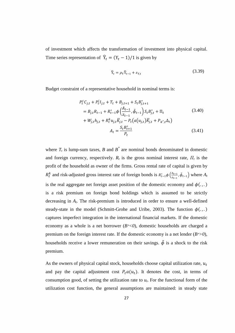
Budget constraint of a representative household in nominal terms is:

1�v[�,� + 1�,��,� + �� + ��,��� + ����,���∗= ��,�A��� + A���∗ 6�z���5��� , 6����� ����,�∗ + Π�+@�,�ℎ�,� + A�B��,����,� − 1�\�\��,�]���,� + 1B�,�∆�]

(3.40)

z� = ������∗1� (3.41)

where Tt is lump-sum taxes, B and B* are nominal bonds denominated in domestic

and foreign currency, respectively. Rt is the gross nominal interest rate, Πt is the

profit of the household as owner of the firms. Gross rental rate of capital is given by

A�B and risk-adjusted gross interest rate of foreign bonds is A���∗ 6 �����8��� , 6����� where At

is the real aggregate net foreign asset position of the domestic economy and 6�. , . � is a risk premium on foreign bond holdings which is assumed to be strictly

decreasing in At. The risk-premium is introduced in order to ensure a well-defined

steady-state in the model (Schmitt-Grohe and Uribe, 2003). The function 6�. , . � captures imperfect integration in the international financial markets. If the domestic

economy as a whole is a net borrower (B∗<0), domestic households are charged a

premium on the foreign interest rate. If the domestic economy is a net lender (B∗>0),

households receive a lower remuneration on their savings. 6� is a shock to the risk

premium.

As the owners of physical capital stock, households choose capital utilization rate, �� and pay the capital adjustment cost 1������. It denotes the cost, in terms of

consumption good, of setting the utilization rate to ut. For the functional form of the

utilization cost function, the general assumptions are maintained: in steady state

28

a(1)=0, u=1 and a’=rk. In production, Kt is used which is transformed from physical

capital ��� according to

�� = ����� (3.42)

Households solve the following maximization problem and choose ?[�,�, ��,���, ���,���, ��,�, ��,�, ��,���∗ , ℎ�,�, ∆�E:

NO� Mu�vw>\[�,� − x[�,���] − u�yz{ ℎ�,���|}1 + ~{Y�W + ν� �A�����,� + A���∗ 6 �z���5��� , 6����� ����,�∗ + Π� +@�,�ℎ�,�

+ A�B��,����,� − 1�\�\��,�]���,� + 1B�,�∆�] − 1�v[�,� − 1�,��,�− �� − ��,��� − ����,���∗ �+ ω� ��1 − �����,� + ��,�Υ� �1 − � � �������� + ∆� − ���,����_

(3.43)

There is unit-root technology in the model, so the solution requires stationarizing the

variables with the technology level such that all real variables are divided by zt and

the multipliers are multiplied by zt. The stationarized variables are written in small

letters (as shown in (3.73), for any real variable X, xt=Xt/zt). Moreover, there exists

unit-root in the price level and some of the variables (e.g. aggregate nominal wage,

rental rate of capital) contain a nominal trend as well. To remove this nominal trend,

those variables are divided by the price level.

The first order conditions for the household’s optimization problem are as follows:

w.r.t. ct:

���v������� �:,�⁄ − Ox �����v����:,������� − �8,� ����� = 0 (3.44)

w.r.t. bt+1:

−�8,� +�8,��� 8,��� A�Π��� = 0 (3.45)

w.r.t. kt+1:

−�8,�1B�� + O�8,��� 8,��� ��1 − ��1B���� + ¡���B ���� − �������� = 0 (3.46)

29

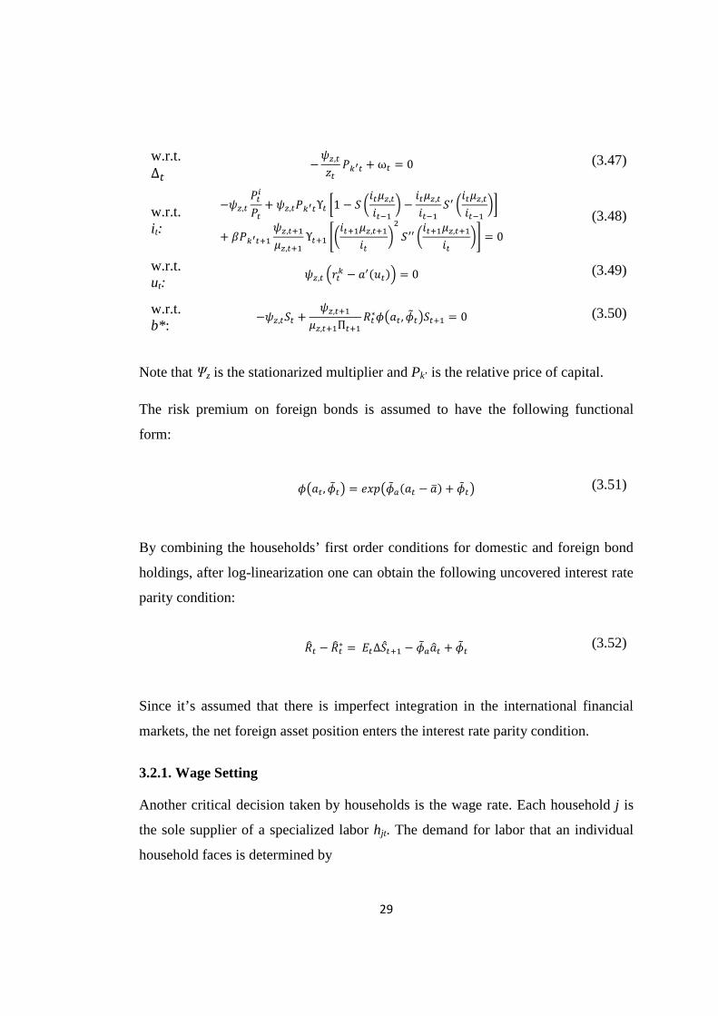
w.r.t. ∆� −�8,�5� 1B�� + ω� = 0 (3.47)

w.r.t. i t:

−�8,� 1�,1� + �8,�1B��Υ� �1 − � �.� 8,�.��� � − .� 8,�.��� �¢ �.� 8,�.��� ��+ O1B�����8,��� 8,��� Υ��� `�.��� 8,���.� �£ �¢¢ �.��� 8,���.� �a = 0

(3.48)

w.r.t. ut:

�8,� �¡�B − �¢����� = 0 (3.49)

w.r.t. b*:

−�8,��� + �8,��� 8,���Π��� A�∗6\�� , 6��]���� = 0 (3.50)

Note that Ψz is the stationarized multiplier and Pk’ is the relative price of capital.

The risk premium on foreign bonds is assumed to have the following functional

form:

6\�� , 6��] = ¤¥¦\6�§��� − �� + 6��] (3.51)

By combining the households’ first order conditions for domestic and foreign bond

holdings, after log-linearization one can obtain the following uncovered interest rate

parity condition:

Al� − Al�∗ = L�∆�g��� − 6�§�b� + 6�� (3.52)

Since it’s assumed that there is imperfect integration in the international financial

markets, the net foreign asset position enters the interest rate parity condition.

3.2.1. Wage Setting

Another critical decision taken by households is the wage rate. Each household j is

the sole supplier of a specialized labor hjt. The demand for labor that an individual

household faces is determined by

30

ℎ�,� = �@�,�@� ���,�����,� �� (3.53)

The model incorporates real rigidities and allows for wage stickiness. Every period

with G% probability, households cannot set their wage optimally but index it to last

period’s CPI inflation rate H�v, the current inflation target H���J , an adds a technology

growth factor to their wage:

@�,��� =  8,���@�,��H�v�I� �H���J ���I� (3.54)

Remaining �1 − G%� fraction of the households set their wage optimally by

maximizing

L�N�G%O�P©ªªª« −u��Py z{ ℎ�,��P��|}

1 + ~{+ℎ�,��Pυ��P�H�v …H��P��v �I��H���J …H��PJ ���I�\ 8,���… 8,��P]@ST%�,�­®®®Y

�W (3.55)

The log-linearized real wage equation is given by:

°���±� +°�����± +°�����±£ + ±²�Hb�/ − Hb�J� + ±²�Hb���/ − &dHb�J�+ ±³�Hb���v − Hb�J� + ±´�Hb�v − &dHb�J� + ±µ�l8,�J+ ±¶��� + ±��·g�y = 0

(3.56)

3.3. The Government

The model assumes that government expenditures are given exogenously as an

AR(1) process:

¸� = &¹¸��� + '¹,� (3.57)

31

3.4. The Central Bank

Monetary policy follows the following instrument rule (in log-linear form):

Al� = &ºAl��� + �1 − &º�\Hb�J + ¡d�Hb���v − Hb�J� + ¡»¼b���+ ¡p¥b���] + ¡½dΔHb�v + ¡½»Δ¼b� + 'º,� (3.58)

where Al� is the short-term interest rate, Hb�v is the CPI inflation rate and ¼b� is the

output gap. The output gap is measured as the deviation from the trend value of

output in the economy as in ALLV (2007), and thus not as the deviation from the

flexible price level as in Smets and Wouters (2003) or JPT (2010).

¥b� is the log-linearized real exchange rate, which is given by

¥b� = �g� + 1l�∗ − 1l�v (3.59)

Hb�v is the model-consistent measure of the CPI inflation rate index:

Hb�v = R�1 − �v�01�1�v2��q� Hb�/ + �v 01�h1�v 2

��q� Hb�h^ (3.60)

Hb�J is the time-varying inflation target which can be referred as inflation target

shock:

Hb�J = &dHb���J + 'd¿�À (3.61)

3.5. Foreign Economy

The foreign inflation, output and interest rate are exogenously described by the

following equations:

Hb�∗ = &d∗Hb���∗ + 'd∗,� (3.62)

32

¼�∗ = &»∗¼���∗ + '»∗,� (3.63)

A�∗ = &º∗A���∗ + 'º∗,� (3.64)

3.6. Market Clearing Conditions

To close the model, equilibrium in good market requires that the production of the

final good be equal to the sum of total spending and the capital utilization adjustment

cost:

[�/ + ��/ + Á� + no� + �������� ≤ 3��,,�4 �5��,,����4 − 5�6 (3.65)

In stationary form the resource constraint is:

�1 − �v�01�v1�2

q� e� + �1 − �,�01�,1�2q� .� + ¸� + 01�p1�∗2

�qr ¼�∗≤ 3�Ã�4 0 1 8,�2

4 ������4 − 6 − ����� Ã� 8,� (3.66)

Foreign bond market clears such that net foreign assets evolve according to:

������∗ = ��1�pno� − ��1�∗�[�h + ��h� + A���∗ 6\����, 6����]����∗ (3.67)

3.7. Relative Prices

Various stationary relative prices enter the model. First is defined in terms of the

imported good. That is, the relative prices between domestically produced goods and

imported goods perceived by the domestic agents. Contrary to ALLV (2007) model,

there is only one domestic relative price since the domestic agents face same price

on the imported consumption goods and the imported investment goods:

33

�h,/ = 1�h1� (3.68)

In addition, the following relative prices are important for households when

determining their consumption and investment baskets:

�v,/ = 1�v1� (3.69)

�,,/ = 1�,1� (3.70)

The relative price between the domestically produced goods (home exports) and the

foreign goods governs the export demand:

Ä�p,∗ = 1�p1�∗ (3.71)

Consequently marginal cost function for the importing firm can be written as:

=e�h = ��1�∗1�h = 1Ä�h,/Ä�p,∗ (3.72)

3.8. Model Solution

In the model, consumption, investment, capital, real wages and output fluctuate

around a stochastic balanced growth path, since the level of technology zt has a unit

root. Because of the permanent technology shock and the unit-root in the price level,

a number of variables are non-stationary as they contain a nominal and real

stochastic trend. Therefore, the solution involves the following steps. First, to render

stationarity of all variables, one needs to divide all quantities with the trend level of

technology zt. and multiply the Lagrangian multiplier with it. Kt and ��� are

34

stationarized with zt-1 whereas the other real variables with zt.. Following Adolfson et

al. (2005) the variables are stationarized in the following way9:

e� ≡ [�5� , ¡�B ≡ A�B1� , °�� ≡ @�1�5� , Ã��� ≡ ����5� , Ã��� ≡ �����5� , ¼�∗ ≡ +�∗5� (3.73)

This way, the model is written in terms of stationary variables. Second, the non-

stochastic steady state of the transformed model is computed and the model is log-

linearly approximated around this steady state10. By linearly approximating the

model, a state-space representation is obtained so that the DSGE model can be

analyzed with the utilization of the Kalman filter. That’s why linear approximation

methods are very popular in the context of likelihood-based DSGE model

estimation. The model is completed by defining a set of measurement equations that

relate the endogenous variables of the model to a set of observables.

9 The domestic and foreign variables stationarized with same level of technology. By doing so, it’s aimed to avoid adding the asymmetric technology shock since variables in our data set cannot pin down this shock and this may lead to under-identification problem. 10 See Appendix A for the linear system of equations.

35

CHAPTER 4

DATA AND METHOD

The DSGE model in this thesis is estimated for Turkish economy with Bayesian

econometric techniques. This chapter presents a review of Bayesian estimation

techniques and presents a description of the data used in the estimation process.

4.1. Data

There exist fourteen exogenous shocks in the model economy. The estimation is

done with fourteen observable variables so that there exist as many observed

variables as shocks to avoid stochastic singularity and identification problems11.

In line with the existing literature, the following key macroeconomic data series are

tried to match: the growth rates of Gross Domestic Product (GDP), consumption,

investment, imports, exports, foreign GDP, and the real exchange rate as well as the

levels of the domestic policy and foreign interest rates; the inflation rates of domestic

GDP deflator, core consumer price (the H-index defined by TURKSTAT) and

import and export prices together with foreign consumer price indices. Regarding the

foreign variables, for real GDP, Euro area GDP is used since the Euro area is

Turkey’s largest trading partner. For interest rate, and inflation rate, U.S. data are

used.

To align the data with the model-based definitions, standard transformations are

applied. For example, all interest rates are divided by four so that the periodic rates

are consistent with the quarterly time series. In addition, in order to make observable

11 Stochastic singularity is the problem of having a case when number of shocks is less than that of the observables. Similarly having less number of observable variables than that of the shocks is not desired since this leads to weak identification of the shocks.

36

variables consistent with the corresponding model variables, the data are demeaned

by removing their sample mean, with the exception of inflation and interest rates,

which are demeaned by subtracting their steady-state values.

The baseline estimation covers the period 2002:2-2011:3. Although the data set

could be extended up to 1987, I chose to start the estimation from 2002 to capture

the episode when the Central Bank of Turkey (CBRT) began to implement an

inflation targeting regime (initially implicitly, and explicitly starting in 2006). This

way, I tried to avoid spurious inference by excluding the periods where regime

changes and structural breaks were observed.

4.2. Method

The method followed for the solution and estimation of the model discussed in

Chapter 3 briefly involves two steps: first the model is solved and written in state-

space form. Then the log-linear system is estimated by Bayesian techniques.

Solving the model means writing the whole system in terms of lagged variables and

current shocks. The coefficients in the DSGE model are structural and are often

complicated functions of underlying preferences and technology. Therefore there is a

high degree of nonlinearity in solution of the model with respect to the parameters.

Hence solving the model requires linearization around a well-defined steady state.

As a second step, the log-linear system is estimated by Bayesian techniques.

The reduced form of the model is given by the following state-space form:

¥� = Á�Æ�¥��� +Z�Æ�'� (4.1)

¼� = ��Æ�¥� (4.2)

Here xt is the vector of endogenous variables written as log deviations from the

corresponding steady state values, εt is the vector of structural shocks and θ is the

vector of parameters. Equation (4.1) is the state/transition equation which describes

37

the evolution of model’s endogenous variables. Equation (4.2) is the observation

equation where yt represents the set of observable variables.

Advantage of working with a log-linear model is that it allows one to simulate the

dynamic response of the model variables to exogenous shocks and calculate

descriptive statistics for all the variables in the model. Moreover, once written in

linear state-space form, there are various ways of estimating or calibrating the

parameters of a DSGE model. Geweke (1999) distinguishes between the weak and

the strong econometric interpretation of DSGE models. The weak interpretation is

built upon calibration and matching data moments or more generally aims to

minimize the distance between empirical and theoretical impulse response functions.

In this approach, the parameters of a DSGE model are calibrated in such a way that

selected theoretical moments given by the model match as closely as possible those

observed in the data.

The strong econometric interpretation on the other hand, attempts to provide a full

characterization of the observed data series. Following Sargent (1989), a number of

authors have estimated the structural parameters of DSGE models using classical

maximum likelihood method. As discussed in detail by Smets and Wouters (2003),

the classical maximum likelihood methods involve using the Kalman filter to form

the likelihood function after writing the model in its state-space form and the

parameters are estimated by maximizing the likelihood function. Alternatively

within this strong interpretation, a Bayesian approach can be followed to estimate

and evaluate DSGE models by combining the likelihood function with prior

distributions for the parameters of the model, to form the posterior density function.

Leading examples of such a Bayesian approach are Otrok (2001), Fernandez-

Villaverde and Rubio-Ramirez (2004), and Schorfheide (2000), Smets and Wouters

(2003).

Following the literature, this thesis uses Bayesian estimation techniques for

estimating the developed DSGE model with the aim of analyzing the sources of

business cycle movements in Turkey. This approach is chosen to include additional

38

information to the estimation process by using prior information over the structural

parameters so that the highly nonlinear optimization algorithm becomes more stable.

This is particularly valuable when only relatively small samples of data are available

(Smets and Wouters, 2003), as is the case with Turkish time series.

To implement rules resulting from agents’ optimization problems, there is need to

determine objects including mean or variance of the parameters -E(θ) or Var(θ). In

particular in Bayesian analysis, the interest is to obtain the entire distribution of θ

conditional on the available data, p(θ│Y). The existence of p(θ│Y) reflects the basic

assumption of Bayesian approach that parameters are random variables with a

probability distribution, whereas classical econometric analysis treats parameters as

fixed, but unknown quantities.

The likelihood function of the observed data series, p(Y│θ), is evaluated with the

Kalman filter. Bayesian approach involves combining this likelihood function, with

prior distributions for the structural parameters of the model, θ. The prior

distribution p(θ) describes the available information prior to observing the data and

summarizes information from other datasets not included in the estimation sample or

economic theory. The observed data, Y, is then used to update the prior, via Bayes

theorem, to the posterior distribution of the model’s parameters, p(θ│Y). Hence one

can think of Bayesian inference as an update of beliefs (Primiceri, 2011). The

posterior is proportional to the product of the likelihood and the prior:

¦�Æ|¼� ∝ ¦�¼|Æ�¦�Æ) (4.3)

The posterior is then optimized with respect to the model parameters either directly

or through Monte-Carlo Markov-Chain (MCMC) sampling methods12. The objective

of MCMC methods is describing the distribution of the posterior by taking draws

from it. In general, the Metropolis–Hastings algorithm, which is a MCMC method, is

used for obtaining a sequence of random samples from a probability distribution for

12 Before posterior simulation, the posterior is maximized numerically with respect to θ, to find the maximum for initializing MCMC.

39

which direct sampling is difficult. This sequence is then used to approximate the

posterior distribution. Main aim of Metropolis-Hasting algorithm is to sample from

the region with highest probability but also to visit the parameter space as much as

possible. The procedure assumes an initial draw from the posterior and as a first step

a candidate value is drawn. Then kernel of posterior is computed at the initial point

and at the draw. If the jump is uphill, draw is always accepted. If it is downhill, the

draw is kept with some nonzero probability. Then the procedure is repeated from the

first step. To monitor the convergence to an invariant distribution, best thing is to run

multiple chains starting from disperse initial conditions (Primiceri, 2011). The

advantage of MCMC algorithm is that MCMC approximating density changes as

iterations progress so that if mistakes are made at some point, they are not carried to

the next iteration.

In summary, Bayesian inference starts out from a prior distribution that describes the

available information prior to observing the data. The observed data is used to

update the prior to the posterior distribution of the model's parameters, which

combines the prior information on the parameters with the likelihood of the data.

Then, mode of the posterior distribution is estimated by maximizing the log posterior

function. In a second step, the Metropolis-Hastings algorithm is used by generating

draws to get a complete picture of the posterior distribution and to evaluate the

marginal likelihood of the model13.

13 Chib and Greenberg (1995) provide details of Metropolis-Hastings algorithm and Schorfheide (2000) present further details about Bayesian estimation.

40

CHAPTER 5

ESTIMATION This chapter presents the main results in terms of parameter estimates, impulse

responses and business cycle variance decomposition14. Moreover a discussion of

how these results fit in the literature is given by comparing parameter estimates

across studies. It is important to note that although such comparison is potentially

useful, two critical issues should be kept in mind. First, various studies consider

distinct countries and sample periods and the structural features of the economies

investigated are different. For example, estimation sample of this thesis includes the

periods of the recent global financial crisis, while most other studies (except Alp and

Elekdağ, 2011) do not. Second, while most of the models build upon a common

core, important differences between models specifications still remain. In sum,

modeling, sample period, and data differences should be recognized when

comparing posterior estimates across various studies.

Section 5.1 discusses which parameters are calibrated and presents the prior and

posterior values of the estimated parameters. Section 5.2 discusses the empirical fit

of the model and presents an evaluation of the model in terms of data fit. The

variance decomposition results are presented in section 5.3. In this section I will

discuss which shocks are found to be important for business cycle fluctuations in

Turkey. Based on the variance decomposition results, the most relevant shocks are

discussed in detail in Section 5.4 giving a brief intuition for how they propagate in

the economy. Since unit-root and investment-specific technology shocks turn out to

govern most business cycle fluctuations, Section 5.5 focuses on technology shocks

14 To carry out the numerical procedure, the software called Dynare is used in this thesis. Dynare is a collection of Matlab and GNU Octave routines (freely available http://www.dynare.org) which basically solve, simulate and estimate the models with forward looking variables.

41

discussing which of the technology shocks are found likely to matter for business

cycles in the related literature with a particular focus on emerging market economies.

5.1. Model Parameters

In this thesis a combination of calibration and estimation strategy is followed as is

common in the literature. A selected set of parameters are kept fixed from the start of

the estimation15. Most of these parameters can be directly related to the steady-state

values of the state variables and are chosen to pin down key steady state ratios, while

the remaining parameters are borrowed from the related literature. Table 5.1 reports

the calibrated parameters.

The discount factor, β, is calibrated to be 0.9928, which implies an annual steady-

state real interest rate around 3 percent. The depreciation rate, δ, is set equal to 0.035

per quarter, which indicates an annual depreciation on capital equal to 14 percent.

Similarly, α is set to 0.40, which roughly implies a 60 percent steady-state share of

labor income in total output. To match the sample average of the import-output ratio

and the ratios of domestic consumption (and investment) over imported consumption

(and investment), the parameters representing the share of imports in consumption

(ωc) and investment (ωi) are set to 0.25 and 0.23, respectively. This calibration

ensures that the shares of steady-state investment and consumption in total output are

roughly 0.2 and 0.7, which corresponds to the average ratios observed over the

estimation period. The (steady state) government expenditure-output ratio is set

equal to its sample mean of 0.1. The constant in the labor disutility function AL is set

to 7, implying that the agents devote around 30 percent of their time to work in

steady state. Following Christiano et al. (2005) and Alp and Elekdağ (2011), the

labor supply elasticity σL is set to 1. In addition, the parameters capturing the markup

rates in wage setting and price setting for domestically produced goods and for

imported goods are calibrated since these parameters are weakly identified by the

15 This can be considered as giving infinitely strict priors.

42

variables included in the data set. Consistent with Alp and Elekdağ (2011), the

steady state price and wage markups are chosen to be 15 percent, which lies in the 10

to 20 percent range utilized in many other studies. The remaining parameters

including various elasticities of substitution are based on Alp and Elekdağ (2011)

and are also summarized in Table 5.1.

The remaining 39 parameters, which mostly pertain to the nominal and real frictions

in the model, the monetary policy stance, as well as the exogenous shock processes,

are estimated. Table 5.2 shows the assumptions for the prior distribution of the

estimated parameters. The location of the prior distribution of the estimated

parameters corresponds to a large extent to those in Alp and Elekdağ (2011).

General principles guiding the prior distributions are as follows: For all parameters

bounded between 0 and 1, the beta distribution is assumed. This consequently

applies to the nominal stickiness parameters ξ, the indexation parameters κ, the habit

persistence b, and the persistence parameters of the shock processes ρ. For all the

shocks, the prior mean of the autoregressive coefficient is set to 0.8. For parameters

assumed to be positive, such as the standard deviations of the shocks σ, the inverse

gamma distribution is proposed. For the unbounded parameters, the normal

distribution is assumed. This applies for instance to capital utilization cost (σa) and

investment adjustment cost parameters (S”).

In Bayesian analysis of DSGE models, it is challenging to formulate beliefs about

the parameters that govern the law of motion of latent exogenous shock processes.

Therefore to let the data determine the size of the shocks as freely as possible, the

degree of freedom for these parameters are set to 2 as in Adolfson, Laséen, Linde

and Villani (2007), (ALLV, hereafter). While determining the mean of the shock

volatilities, the prior means of the mark-up shocks in domestic and import goods are

set to 0.05. This choice is based on the fact that Turkey is a small economy and is

expected to be subject to large mark-up shocks (ALLV, 2008). Moreover,

considering the low volatility in foreign variables, for the size of the foreign shocks I

43

chose a smaller value of 0.01. For all other shocks prior means are set to 0.03 in line

with Alp and Elekdağ (2011).

The results are reported in Table 5.2. The Table shows the means along with the 5th

and 95th percentiles of the posterior distribution of the estimated parameters obtained

through the Metropolis-Hastings sampling algorithm. The results are based on a total

of 300,000 draws and two independent chains, and the Brooks and Gelman (1998)

convergence criteria are achieved. The parameter draws are converted into variance

decompositions to obtain the results presented in Table 5.3. Additional information

on the estimation results is presented in Figure 5.1a through Figure 5.1d, which plot

the prior and the posterior distributions for the estimated parameters. A direct

comparison of priors and posteriors can provide valuable insights about the extent to

which data provide information about the parameters of interest. These figures

provide a visual summary indicating that the data are quite informative regarding

most of the estimated parameters.

The Calvo parameter for domestic goods is found around 0.66 which implies

domestic prices are adjusted on average every 3 quarters. The degree of domestic

price stickiness is higher than the value found in Alp and Elekdağ (2011) and lower

than ALLV (2008). But as Özmen and Sevinç (2011) points out price stickiness in

Turkey is time and state dependent and there is great heterogeneity across groups,

which makes comparison of the findings of different studies difficult. The degree of

wage stickiness parameter is around 0.75, implying wages are adjusted every 4

quarters, on average. The degree of stickiness in import sector is higher than that of

domestically produced goods which is consistent with the findings of Alp and

Elekdağ (2011). But the ALLV (2008) finds a reverse order suggesting import good

prices are less sticky than domestic good prices. The indexation parameters (i.e. the

κ’s) are around 0.5 which implies the Philips curve has significant backward looking

components. Regarding the history of high inflation periods in Turkey, importance

of backward looking behavior is meaningful. These indexation parameter values are

higher than those found in ALLV (2008), suggesting that the estimated Phillips

44

curves for Sweden are relatively more forward-looking, as expected. The results

indicate that the unconditional variance of the markup shocks in the import sector is

considerably higher than in the domestic sector.

Comparison of estimated policy rules turns to be challenging since various studies

focus on different specifications. The specification in this thesis is similar to that of

ALLV (2007). The interest rate smoothing parameter, which is found to be 0.7, is in

line with many other studies. As for the responsiveness of inflation deviation from

target, the estimated value of 1.42 is close to the values of 1.5 and 1.6 found by Alp

and Elekdağ (2011) and ALLV (2007), respectively. The responsiveness to the real

exchange rate depreciation is smaller echoing the findings of Alp and Elekdağ

(2011). The responsiveness of policy rates to the output gap takes on a lower value

of 0.08. This value should not be misleading. Although the interest rate rule

coefficient implies a small systematic response of policy rate to output gap, it is

known that Central Bank of Turkey responded to the large output drops during the

crisis through discretionary departures from the rule. Hence the importance given to

output gap deviations may not be properly captured with these parameters (ry and

rdy).

Turning to exogenous shocks, I start off by discussing persistence parameters. The

estimated persistence parameters lie within the range of 0.3 for the foreign inflation

shock, and 0.93 for the foreign interest rate shock. A caveat should be made here. As

will be discussed in model fit section, the model does not perform persuasively

enough at fitting the foreign variables, hence these parameter values should be

interpreted with highest caution.

The posterior mode of the persistence parameter in the unit-root technology process

is estimated to be 0.55. In addition, the persistence coefficient for the stationary

technology shock is estimated to be around 0.77. These values compare quite

favorably to the estimates in Alp and Elekdağ (2011). As for standard deviations, the

foreign interest rate shock is the least volatile, whereas the variability of the

preference, exogenous spending and import mark-up shocks are noteworthy. It may

45

also be useful to point out that as in other studies (Alp and Elekdağ, 2011, ALLV,

2007), the unit-root technology shock is more volatile than the stationary technology

shock. As will be discussed in further detail in Section 5.3, in terms of driving the

business cycle, it’s expected to see that the unit-root technology shocks plays a much

more prominent role. This finding is consistent with the theoretical predictions of

Aguiar and Gopinath (2007) which emphasizes the fact that shocks to trend growth

are the primary source of fluctuations in developing countries rather than transitory

fluctuations around a stable trend.

5.2. Model Fit

Model evaluation is an important part of the empirical work that is based on DSGE

modeling. Figure 5.2 reports the model’s one-sided Kalman filter estimates of the

observed variables along with the actual variables. Such a comparison is informative

in terms of assessing the fit of the model.

As is evident from Figure 5.2, the in-sample fit of the model is satisfactory.

However, the model is not good at capturing exports and other foreign variables. In

this thesis, the foreign variables are modeled as exogenous AR(1) processes. Such a

specification does not incorporate the fact that these foreign variables (i.e. foreign

demand and foreign interest rate) are highly correlated with each other. An

alternative to the modeling approach here would be modeling the foreign economy

as a VAR model as in ALLV (2007), because the assumed structure does not capture

the evolution of foreign economy as properly16. As a consequence, the model falls

somewhat short in capturing the export dynamics, which is closely related to the

modeling assumptions of the foreign economy. This in turn weakens the fit of output

to a certain extent. As is clear in Figure 5.2, the model is quite good in capturing

main components of output including consumption, investment and imports.

16 However, since the main question of this thesis does not focus on foreign variables (or related shocks), this does not constitute a serious problem.

46

5.3. Shocks and Business Cycles

This section analyzes the driving forces of fluctuations by looking at the variance

decomposition of the main macroeconomic variables implied by the estimated

model. To make a formal assessment of the contribution of each shock to the

fluctuations of the endogenous observable variables, Table 5.3 reports the variance

decompositions.

The “unit root technology” row of Table 5.3 makes clear that unit-root technology

shocks account for 60 percent of the fluctuations in output, almost 35 percent of

those in consumption and around 47 percent of those in investment; these are by far

the largest shares. Also Figure 5.3 shows that unit-root technology shock accounts

for the bulk of the fluctuations in output. On the basis of this outcome, one can

conclude that unit-root technology shock of the model serves as the leading source of

the Turkish business cycles. This finding is consistent with Aguiar and Gopinath

(2007) which argues that emerging markets are characterized by volatile trend

growth rates and shocks to trend growth constitute the primary source of fluctuations

in emerging markets.

The model in this thesis has two productivity processes, a transitory shock around

the trend growth rate of productivity (Ɛt) and a stochastic trend growth rate (zt). The

intuition for the model’s dynamics is as follows. A positive shock to stationary

technology makes agents increase their consumption and investment spending as

they observe the economy entering a period of high growth. However, a positive

disturbance to unit-root technology implies a boost to current output, but an even

larger boost to future output. This implies that consumption responds more than

income, reducing savings. The literature provides evidence that if growth shocks

dominate transitory income shocks, the economy resembles a typical emerging

market with its volatile consumption process and countercyclical current account.

Conversely, an economy with a relatively stable growth process will be dominated

by standard, transitory productivity shocks (Aguiar and Gopinath, 2007).

47

Motivated by the observed frequent policy regime switches in emerging markets,

Aguiar and Gopinath (2007) argues that these economies are subject to substantial

volatility in the trend growth rate relative to developed markets. The unit-root

technology shock could therefore be considered as associated with changes in

government policy, including changes in monetary, fiscal, and trade policies because

dramatic changes in productivity are observed following reforms and the undoing of

reforms. Consequently, shocks to trend growth are the primary source of fluctuations

in these markets rather than transitory fluctuations around a stable trend. Moreover

the observed predominance of permanent shocks relative to transitory shocks for

emerging markets explains differences in key features of their business cycles

stylized facts. It is well-shown that trend shocks increase the ability of the models to

capture some data facts specific to emerging market economies such as

countercyclicality of net exports and higher volatility of consumption compared to

output (Aguiar and Gopinath, 2007, Akkoyun et al. 2011). Being an emerging

market economy subject to policy changes, one can observe similar business cycle

stylized facts in Turkish economy. As shown in Alp et al. (2012), volatility of

consumption relative to GDP is quite high and net exports show a countercyclical

pattern in Turkey. Moreover Alp et al. (2012) also shows that business cycle

properties of some key macroeconomic variables change in pre- and post-2001

period due to a change in monetary policy and a set of structural reforms which

points to importance of structural changes in Turkish economy17. Therefore finding

unit-root technology shocks, which affect the trend growth rate, as the leading source

of macroeconomic fluctuations in Turkish economy is in line with the suggestions of

the literature.

Looking at the other shocks and variables, two results stand out. First, the investment

shock appears to be fairly important. Together with the exogenous spending shock

they stand as the next set of important shocks in explaining output fluctuations.

Shocks to marginal efficiency of investment (MEI) are important in explaining

output fluctuations. Investment is one of the most volatile components of output 17 See Alp et al. (2012) for a detailed survey of Turkish economy business cycle stylized facts.

48

(volatility of investment relative to output is around 3) in Turkey. Explaining such a

volatile variable requires a high role for the shock that is closely related to

investment. Moreover, this shock is also closely related to financing conditions. As

suggested in Chrisitano et al. (2010) and Justiniano et al. (2011), investment shocks

might proxy for more fundamental disturbances to the intermediation ability of the

financial system since access to credit and financial intermediation are important

determinants of investment. Regarding the high volatility in financing conditions in

Turkey (mainly due to the close relation of domestic credit to the highly volatile

variables such as risk premium and capital flows) investment shock is naturally

expected to play an important role in Turkish business cycles. However, the MEI

shock is found to contribute less than expected and it accounts only for 10 percent of

the fluctuations in output. Compared to the findings of JPT (2010), the role of

investment shocks in explaining business cycles turns out to be less spelled. As

discussed in JPT (2010), part of this conclusion may be related to the measurement

of the observable variables. JPT (2010) argues that main reason why the studies that

find less significant role of investment shocks in business cycles, is the difference in

measurement of investment and consumption series18. In JPT (2010), investment

series includes durable consumption and change in inventories. However, in Turkish

data, there is no explicit time series for durable and non-durable consumption. Hence

consumption series used in the estimation includes purchases of consumer durables

in consumption, whereas JPT (2010) includes durable consumption in investment.

This increases (decreases) the volatility of investment (of consumption) in JPT data

set, compared to a case where durable consumption is included in consumption.

Since Turkish data do not allow for such a differentiation, the way variables are

measured may be resulting in a less volatile investment series than it should be.

Although investment is a highly volatile component of GDP in Turkey, it may be the

case that including durable consumption in investment may help to have a higher

role for investment shocks as such inclusion would add up to the existing volatility

18 Smets and Wouters (2003), for instance is one study that reports a lower effect for investment shocks in business cycles.

49

of investment. For model dynamics relative volatility of the variables does also

matter. Such measurement of investment would add up to the volatility of

investment relative to that of GDP as well. Hence, a higher volatility of investment

might be necessary to have a higher role for investment shocks since the Turkish real

GDP series is also volatile. As Guerron-Quintana (2010) points out the estimation

results are quite sensitive to the used data. Another reason why investment shocks

turn to play a minor role can be related to the impulse response analysis. As evident

in Figure 5.5, investment shock leads output and consumption to move in opposite

directions. Although model incorporates all the mechanisms that are proposed to be

important for transmission of investment shocks, the estimated model does not

generate the comovement of output and consumption. Given the strongly positive

correlation of output and consumption over the business cycle in Turkey (Alp et al.,

2012, this implies that investment shocks cannot play a leading role in the business

cycles as given by the variance decomposition analysis.

Another outcome that needs to be focused is the leading role of preference shocks in

explaining consumption path. The preference shock is an intertemporal disturbance,

which perturbs the agents’ intertemporal first order conditions. This can be

considered as a shock to the stochastic discount factor, which captures exogenous

fluctuations in preferences, as well as unmodelled distortions in consumption

choices. The leading role of this shock in explaining consumption is a symptom of

the well-known failure of standard consumption Euler equations to capture the

empirical relationship between consumption and interest rates, as argued in Primiceri

et al. (2005). Intuitively, large exogenous variations in the stochastic discount factor

are necessary to repair the poor performance of the standard Euler equation.

Therefore, a large taste shock bt is necessary to reconcile the interest rates with the

growth rate of consumption. Especially in case of Turkey where the volatility of

consumption is quite high (even as high as that of output, as discussed in Alp et al.,

2012), there is need for a large preference shock to explain the observed

consumption volatility. That’s why the estimation results indicate such a big role for

preference shocks.

50

5.4 Model dynamics and shock identification

The variance decomposition analysis identifies that permanent technology and

investment shocks explain bulk of the variation in output observed in Turkey.

Therefore, the results of this thesis suggest that to understand business cycles in

Turkish economy, one must understand permanent technology shocks and

investment shocks, since these shocks are the largest contributors to fluctuations in

several key macroeconomic variables. This section provides some intuition for how

this identification is achieved, by studying the impulse responses of several key

variables to some of the shocks. In particular, I focus on the two shocks that are

responsible for the bulk of fluctuations according to estimation results: the

investment shock and the unit-root technology shock. Figures 5.4 and 5.5 report the

impulse responses to these shocks.

Figure 5.4 reports the impulse responses to unit root technology shock. Following a

positive impulse, output, consumption and investment all rise. The reaction in

investment is contemporaneous and roughly proportional to that in output, but larger.

Real wages are also procyclical. The response of hours is very similar to that of

output.

Figure 5.5 reports the impulse responses to investment shock. As evident in Figure

5.5, investment shocks trigger procyclical movements in all key macroeconomic

variables. Following a positive impulse, output, hours and investment all rise. But

the movement of consumption reminds the Barro-King (1984) critique. It shows a

drop and remains flat, and rises after a long time. Finally, inflation and the nominal

interest rate, both rise in response to a positive investment shock. The investment

shock leads to a situation where output and investment moves in opposite directions

and cannot create the comovement of consumption and output. In terms of

comovement, the Barro-King (1984) critique applies.

51

5.5 Discussion: The role of technology and investment shocks

A central question in macroeconomics concerns the role of technology shocks in

driving business cycle fluctuations. The evidence generated by the literature does not

speak with a single voice and conclusions do vary. The first line of research (the

early RBC literature) argues that technology shocks are the primary drivers of

business cycles. A second line of literature pioneered by Gali (1999) questions the

view of technological change as a central force behind cyclical fluctuations and

concludes that technology shocks are largely irrelevant. Finally a relatively recent

line of research including much of the estimated DSGE literature arrives at

conclusions somewhere in between these two extremes (Fisher, 2006, and Smets and

Wouters, 2007).

In this section I will discuss how the main findings of this thesis fit in this part of the

literature, which discusses the relative importance of technology and non-technology

shocks. While doing this, I will focus on role of three different technology shocks:

First is the covariance stationary technology shock which does not affect long-run

trend of productivity. The second is the permanent (or unit root) technology shock

which does matter for long-run productivity level. The third is the investment shock

which is either specified as a shock that affects transformation of consumption goods

into investment goods (i.e. the investment-specific technology shock popularized by

Greenwood et al., 1988) or as a shock that affects the transformation of investment

goods into effective capital stock (i.e. the marginal efficiency of investment shock).

Neutral technology shocks are classified into two: First type is a transitory

technology shock that can potentially capture a variety of driving forces behind

output and labor input fluctuations that would not be expected to have permanent

effects on labor productivity. This is the benchmark supply shock which has been

attributed a central role in the RBC literature as an important source of business

cycle fluctuations. Second is a particular type of shock to trend growth, which has a

permanent impact on labor productivity. This shock is also referred to as a unit-root

technology shock. Pioneered by Aguiar and Gopinath (2007), this type of trend

52

shock is considered as a key determinant of business cycle fluctuations across

emerging markets.

Stationary and permanent technology shocks affect the aggregate production level

whereas the third technology shock (i.e. investment shock) affects only

transformation of investment goods. However, the channels these technology shocks

affect the economy are similar. A positive shock to either of these leads to a rise in

productivity and in output. But owing to the permanent nature of the shock, unit-root

technology shock affects the long-run trend of productivity and its transmission is

stronger. All real variables are affected strongly by the unit-root technology shock

(Table 5.3). The effect of the stationary technology (ST) shock on output appears to

be weaker compared to its unit-root counterpart. Moreover the fact that hours falls in

response to a positive stationary technology shock is found to be problematic (Gali,

1999). Therefore as consistent with the findings in the literature, I find a negligible

role for ST shock in explaining output fluctuations in Turkey. For example ALLV

(2005), finds that at small frequencies (20 quarters) unit root technology shock

explains 25 percent of the variations in output whereas the role of ST shock is

limited (4 percent). In JPT (2010) ST shock is not even considered in the model and

the unit-root technology shock is assumed to be the sole source of neutral technology

shock which explains 25 percent of the U.S. output fluctuations at business cycle

frequencies. One can conclude that the findings in the literature agree regarding the

negligible explanatory role of ST shocks in business cycles. Rather, a lively debated

issue in the literature is the relative role of unit-root technology and investment

shocks in explaining output fluctuations.

The identification of investment specific technology shock, which hits the

transformation of investment goods into capital goods, is an important part of the

discussion. Some existing studies try to identify this shock by equating it to the

relative price of investment (e.g. Altig et al., 2005). JPT (2011) argues that in

addition to this identification, the investment shock has another source related to

marginal efficiency of investment (MEI) which is not related to relative prices.

53

Therefore they point out that two sources of investment shock should be

distinguished. But as is done in this thesis, most other studies, including Smets and

Wouters (2007), ALLV (2007) and JPT (2010), treat the two disturbances as a

unique unobservable shock19. Specified in this way, I find that main driving force of

business cycles in Turkey is the unit-root shock whereas contribution of investment

shock is also significant, but limited. Regarding the relative importance of unit-root

technology and investment shocks, this finding is different from JPT (2010), which

concludes MEI shock explains around 50 percent of output fluctuations. In an open

economy setting, ALLV (2007) finds that in explaining output variations, unit-root

technology shock has a higher explanatory role (25 percent) than that of investment

shock (12 percent) which is quite comparable to the findings of this thesis. Similarly,

Alp and Elekdağ (2011) finds that unit root technology shock is the most important

supply shock in terms of output growth contributions in Turkey which is consistent

with the findings of this thesis. Therefore, modeling the economy as an open

economy seems to affect the importance of MEI shock.

One could also compare the results of this thesis with that of similar studies on

developing small open economies. It is important to discuss how and why the

importance of the three types of technology shocks, as sources of business cycles in

developing economies, changes compared to the developed economies.

Emerging market economies have different business cycle stylized facts summarized

by countercyclical net exports and highly volatile consumption. These features

contrast with developed economies and constitute a unique case of emerging

markets. Trying to capture these unique patterns in a dynamic stochastic small open

economy model, Aguiar and Gopinath (2007) highlights the fact that these

economies are subject to substantial volatility in the trend growth rate relative to

developed markets and concludes shocks to trend growth are the primary source of

19 Investment disturbance in this thesis refers to MEI shock. Such specification is still appropriate as Justiniano et al. (2011) finds that, contribution of IST shock identified with relative price of investment, is negligible whereas MEI shock remains to play a key role in U.S. business cycles as previously shown in Justiniano et al. (2010).

54

fluctuations in developing countries rather than transitory fluctuations around a

stable trend. The findings of the studies examining sources of business cycles in

developing economies within a DSGE setting are in line with the suggestions in

Aguiar and Gopinath (2007). For instance Medina and Soto (2007) finds that unit

root technology and investment shocks explain around 50 percent of output

variations in Chile. Moreover there are various studies which show that modeling

emerging market economies as an economy subject to trend shocks helps to better

capture the data facts of these countries20.

The above-mentioned findings of the literature suggest that although relative

contributions are different, unit-root technology and investment shocks play a key

role in business cycles. Moreover these two shocks create a similar movement in

endogenous variables except consumption (Figures 5.4 and 5.5). Comparing the

cumulative effects of the three types of technology shocks may give a better picture

regarding the role of technology in explaining business cycles. JPT (2010) finds the

total effect of technology (unit-root technology and MEI shocks) in variations of

U.S. output as 70 percent. I find that technology shocks (unit-root technology, ST

and MEI shocks) explain around 75 percent of the output fluctuations. Adding an

asymmetric technology shock ALLV (2007) concludes that technology shocks

explain around half of output fluctuations in Euro area. Such a comparison shows

that the results of this thesis regarding the high role of technology shocks are

consistent with the literature.

Finally, comparing the findings of this thesis with the results of other estimated

models of the Turkish economy is also informative. To the best of my knowledge,

Alp and Elekdağ (2011) is the only study that estimates a DSGE model for Turkey

with Bayesian estimation methods for a similar sample period. Their model

incorporates a richer set-up with financial accelerator mechanism. Throughout the

estimation, I use this study as a benchmark while determining priors and analyzing

estimation results. Turning to the business cycle implications of Alp and Elekdağ

20 See Akkoyun et al. (2011) and Arslan et al. (2012).

55

(2011), they do not provide the variance decomposition but presents historical

decomposition to understand the contributions of the structural shocks to output

growth. They find that two prominent supply shocks are the unit-root and

investment-specific technology shocks. Although they find investment shocks to be

important, they emphasize that the unit root technology shock seems to be the most

effective supply shock in output growth echoing the findings of this thesis. Similar to

this thesis, they find limited role for the cost push (markup) and stationary

technology shocks.

Turning to data may give some clue about why role of investment shocks in

explaining business cycles in Turkey are found to be limited in this thesis compared

to findings for U.S. (JPT, 2010 and 2011). Figure 5.6 shows the relative price of

investment together with GDP, consumption and investment price deflator. Figure

5.7 shows relative price of investment in U.S. as given in JPT (2011). In this thesis

investment shock can be considered as a combination of investment specific

technology shock, which is identified through relative price of investment and

marginal efficiency of investment shock, which is related to financing conditions

(JPT, 2011). Hence this figure can give some idea about the total role of investment

shocks (JPT, 2011).

As evident from Figure 5.6, investment price deflator stays below GDP deflator for

the whole sample and relative price of investment shows a downward pattern. But

relative investment price seems to oscillate within 0.8- 1.1 range rather than showing

a clear downturn as observed in U.S (Figure 5.7). Since part of the investment shock

is related to the inverse of relative investment price, one would expect to see a more

clear downward pattern if investment shocks were dominant in the sample period.

Hence this figure does not give much hint about importance of investment shock in

Turkey as is found in U.S.

56

CHAPTER 6

CONCLUSION

Understanding sources of business cycles has been has been central in the public and

academic debates for long periods. For different countries, different sources emerge

to be important for explaining output fluctuations. In emerging market economies

unit-root technology shocks are found to be the driving force of macroeconomic

fluctuations whereas for developed economies in addition to such productivity

shocks investment and mark-up shocks are found to matter. Inspired by this line of

research, this thesis investigates sources of output fluctuations and conducts a test

for the role of various shocks in Turkish economy by looking at variance

decomposition results obtained by estimating a small open economy DSGE model

by Bayesian methods. Employing this method not only allows the data speak but

also enables to take the advantage of using prior information about the economy

which is valuable while working with short data samples.

The results show that unit root technology, investment and exogenous spending

shocks explain around 75 percent of output fluctuations in Turkish economy for the

period 2002:2-2011:3. The unit root technology shock appears to be the key driving

force of business cycles as this shock accounts for more than half of the

macroeconomic fluctuations. The result that unit-root technology shock, which

affects trend growth rate, is the key driver of business cycles indicates the

importance of permanent shocks such as policy changes and structural reforms in

Turkish economy.

This thesis uses state-of-art modeling and estimation techniques, which are proven to

be useful in the literature. However, there are a number of dimensions in which the

model can be improved. First, the foreign economy is assumed to be exogenously

57

determined and all foreign variables are assumed to follow an AR(1) process. The

weakness of the model to capture movement of foreign economy variables observed

in the data indicates the need of a more structural modeling of foreign economy as is

done in Adoolfson et al. (2007). Second, the treatment of fiscal policy in the model

is very simplistic. Enriching the fiscal part of the model would be interesting as it

would allow studying the interaction between monetary and fiscal policy in an

empirical model. Third, the model does not include a well-developed financial

sector. Including a banking sector and financial accelerator channel can generate

interesting dynamics in the economy and affect the empirical performance of the

model.

58

REFERENCE

Adolfson, M., S. Laseen, J. Linde and M. Villani (2005) Bayesian Estimation of an Open Economy DSGE Model with Incomplete Pass-Through, Working Paper Series, No. 179, Sveriges Riksbank. Adolfson, M., S. Laseen, J. Linde and M. Villani (2007) Bayesian Estimation of an Open Economy DSGE Model with Incomplete Pass-Through, Journal of International Economics, Vol. 72, 481–511. Adolfson, M., S. Laseen, J. Linde and M.Villani (2008) Evaluating an Estimated New Keynesian Small Open Economy Model, Journal of Economic Dynamics and Control, Vol. 32, 2690–2721. Aguilar, M. and G. Gopinath (2007) Emerging Market Business Cycles: The Cycle is the Trend, Journal of Political Economy, 115(1), 69-102. Akkoyun, H. Ç., Y. Arslan and M. Kılınç, (2011) Trend Shocks, Non-tradables and Real Exchange Rates, mimeo, Central Bank of Turkey. Alp, H. and S. Elekdağ (2011) The Role of Monetary Policy in Turkey during the Global Financial Crisis, Working Paper Series, No.11/10, Central Bank of Turkey. Alp, H., Y.S. Başkaya, M. Kılınç and C. Yüksel (2012) Stylized facts for Business Cycles in Turkey, Working Paper Series, No.12/02, Central Bank of Turkey. An, S. and F. Schorfheide (2007) Bayesian Analysis of DSGE Models, Econometric Reviews, Vol. 26, 113-172. Altig, D., L. J. Christiano, M. Eichenbaum and J. Linde (2005) Firm-Specific Capital, Nominal Rigidities and The Business Cycle, Working Paper Series, No. 11034, NBER.

59

Arslan, Y., G. Keleş and M. Kılınç (2012) Trend Shocks, Risk Sharing and Cross-Country Portfolio Holdings, Working Paper Series, No.12/05, Central Bank of Turkey. Barro, R. J., and R. G. King (1984) Time-Separable Preference and Intertemporal-Substitution Models of Business Cycles, Quarterly Journal of Economics, 99(4), 817-839. Bergin, P. R. (2003) Putting the New Open Economy Macroeconomics to a Test, Journal of International Economics, Vol. 60, 3-34. Bernanke, B. S., M. Gertler and S. Gilchrist (1999) The Financial Accelerator in a Quantitative Business Cycle Framework, Handbook of Macroeconomics, in: J. B. Taylor and M. Woodford (ed.), Edition 1, volume 1, chapter 21, 1341-1393. Brooks, S. P. and A. Gelman (1998) Alternative Methods for Monitoring Convergence of Iterative Simulations, Journal of Computational and Graphical Statistics, 7, 434-455. Calvo, G. (1983) Staggered Prices in a Utility Maximizing Framework, Journal of Monetary Economics, 12, 383-398. Chib S. and E. Greenberg (1995) Understanding the Metropolis-Hastings Algorithm, American Statistician, 49 (4), 327-335. Christiano, L. J., M. Eichenbaum, and R. Vigfusson (2004) What Happens After a Technology Shock?, mimeo, Northwestern University. Christiano, L., M. Eichenbaum, and C. Evans (2005) Nominal Rigidities and the Dynamic Effects of a Shock to Monetary Policy, Journal of Political Economy, Vol. 113, 1-45. Christiano, L. J., R. Motto, and M. Rostagno (2010) Financial Factors in Economic Fluctuations, Working Paper Series, No.1192, European Central Bank.

60

Clarida, R., J. Gali and M. Gertler (1999) The Science of Monetary Policy: A New Keynesian Perspective, Journal of Economic Literature, Vol. 37(4), 1661-1707. DeJong, D. N., B. F. Ingram and C. H. Whiteman (2000) A Bayesian Approach to Dynamic Macroeconomics, Journal of Econometrics, 98 (2), pp. 203-223. Dib, A. (2003) Monetary Policy in Estimated Models of Small Open and Closed Economies, Working Paper Series, No. 2003-27, Bank of Canada. Fernández-Villaverde, J. (2009) The Econometrics of DSGE Models, Working Paper Series, No. 14677, NBER. Fisher, J. D. M. (2006) The Dynamic Effect of Neutral and Investment-Specific Technology Shocks, Journal of Political Economy, 114(3), 413-451. Gali, J. (1999) Technology, Employment, and the Business Cycle: Do Technology Shocks Explain Aggregate Fluctuations?, American Economic Review, 89(1), 249-271. Gali, J., and T. Monacelli (2002) Monetary Policy and Exchange Rate Volatility in a Small Open Economy, Working Paper Series, No. 8905, NBER. Gertler, M., S. Gilchrist, F. Natalucci (2007) External Constraints on Monetary Policy and the Financial Accelerator, Journal of Money, Credit and Banking, Vol. 39(2-3), 295-330. Geweke, J. (1998) Using Simulation Methods for Bayesian Econometrics Models: Inference, Development and Communication, mimeo, Federal Reserve Bank of Minneapolis. Greenwood, J., Z. Hercowitz, and G. W. Huffman (1988) Investment, Capacity Utilization and the Real Business Cycle, American Economic Review, 78(3), 402-417. Greenwood, J., Z. Hercowitz, and P. Krusell (1997)“Long Run Implications of Investment-Specific Technological Change, American Economic Review, 87(3), 342-362.

61

Greenwood, J., Z. Hercowitz, and P. Krusell (2000) The Role of Investment-Specific Technological Change in the Business Cycle, European Economic Review, 44(1), 91-115. Guerron-Quintana, P. A. (2010) What You Match Does Matter: The Effects of Data On DSGE Estimation, Journal of Applied Econometrics, Vol. 25, 774-840. Justiniano, A., G. E. Primiceri and A. Tambalotti (2010) Investment Shocks and Business Cycles, Journal of Monetary Economics, 57(2), 132–145. Justiniano, G. E. Primiceri and A. Tambalotti (2011) Investment Shocks and the Relative Price of Investment, Review of Economic Dynamics, 14(1), 101-121. King, R. G., and S. T. Rebelo (1999) Resuscitating Real Business Cycles, Handbook of Macroeconomics, in: J. B. Taylor and M. Woodford (ed.), Amsterdam. North-Holland. Kydland, F. E., and E. C. Prescott (1982) Time to Build and Aggregate Fluctuations, Econometrica, 50(6), 1345-70. Lane, P. (2001) The New Open Macroeconomics: A Survey, Journal of International Economics, Vol. 54, 235-266. Lubik, T. A., and F. Schorfheide (2007) Do Central Banks Respond to Exchange Rate Movements? A Structural Investigation, Journal of Monetary Economics, Vol. 54, 1069-1087. Lucca, D. O. (2005) Resuscitating Time to Build, mimeo, Board of Governors of the Federal Reserve System. Medina, J. P. and C. Soto (2007) The Chilean Business Cycles Through The Lens Of A Stochastic General Equilibrium Model, Working Paper Series, No.457, Central Bank of Chile.

62

Monacelli, T. (2003) Monetary Policy in a Low Pass-through Environment, Working Paper Series, No.227, European Central Bank. Obstfeld, M. and K. Rogoff (1995) Exchange Rate Dynamics Redux, Journal of Political Economy, Vol. 103, 624-660. Otrok, C. (2001) On Measuring the Welfare Cost of Business Cycles, Journal of Monetary Economics, 47(1), 61-92. Özmen, M. U. and O. Sevinç (2011) Price Rigidity in Turkey: Evidence from Micro Data, Working Paper Series, No.11/25, Central Bank of Turkey. Primiceri, G. E., E. Schaumburg, and A. Tambalotti (2005) Intertemporal Disturbances, mimeo, Northwestern University. Primiceri, G. E. (2011) A Short Course on Bayesian Inference in Macroeconomics, 27-29 June, Central Bank of Turkey. Ravn, M. O. and S. Simonelli (2007) Labor Market Dynamics and the Business Cycle: Structural Evidence for the United States, Scandinavian Journal of Economics, 109(4), 743-777. Sargent, T. J. (1989) Two Models of Measurements and the Investment Accelerator, Journal of Political Economy, 97(2), 251-87. Schmitt-Grohe, S. and M. Uribe (2003) Closing Small Open Economy Models, Journal of International Economics, 61(1), 163-185. Schorfheide, F. (2000) Loss Function-Based Evaluation of DSGE Models, Journal of Applied Econometrics, Vol. 15, 645-670. Shapiro, M. D., and M. Watson (1988) Sources of Business Cycle Fluctuations. NBER Macroeconomics Annual, 111-148, MIT Press, Cambridge, Massachusetts.

63

Sims, E. R. (2011) Permanent and Transitory Technology Shocks and the Behavior of Hours: A Challenge for DSGE Models, mimeo, Stanford University. Smets, F., and R. Wouters (2003) An Estimated Stochastic Dynamic General Equilibrium Model of the Euro Area, Journal of the European Economic Association, 1(5), 1123-1175. Smets, F., and R. Wouters (2007) Shocks and Frictions in US Business Cycles: A Bayesian Approach, American Economic Review, 97(3), 586-606. Woodford, M. (2003) Interest and Prices, Princeton N.J, Princeton University Press.

64

APPENDIX

A. The log-linearized model

In this part of the Appendix, the log-linearized equations in the model are presented.

First, the domestic Phillips curve and the log-linearized marginal costs are given by:

Hb� − Hb�J = O1 + Oc/ �L�Hb��� − &dHb�J� + c/1 + Oc/ �Hb���h − Hb�J�

− c/O�1 − &d�1 + Oc/ Hb�J + �1 − G/��1 − OG/�G/�1 + Oc/� \=ef � + $g/,�] (A1)

=ef � = F¡�B + �1 − F�°��� − 3� (A2)

¡�B =  8,� + °��� + ��� − Ãl� (A3)

The Phillips curves for the imported good is:

Hb�h − Hb�J = O1 + Och �L�Hb���h − &dHb�J� + ch1 + O= �Hb���h − Hb�J�− chO�1 − &d�1 + Och Hb�J+ �1 − Gh��1 − OGh�Gh�1 + Och� \=ef �h + $gh,�]

(A4)

=ef �h = \1l�∗ + m� − 1l�h]

The log-linearized real wage equation can be written

°���±� + °�����± + °�����±£ + ±²�Hb�/ − Hb�J� + ±É�Hb���/ − &dHb�J�+ ±³�Hb���v − Hb�J� + ±´�Hb�v − &dHb�J� + ±µ�l8,�J + ±¶���+ ±��·g�y = 0

(A5)

Investment equation is given by

1B��+Υ�� − γb�,,/ −  8£�¢¢C�Ë� − Ë���� − O�Ë��� − Ë��+μb8,�D − Oμb8,��� = 0 (A6)

65

The log-linearized UIP condition is given by

Al� − Al�∗ = L�∆�g��� − 6�§�b� + 6l� (A7)

The aggregate resource constraint is given by

�1 − �v��Äv,/�q� e¼ �e� + ±vÄb�v,/� + �1 − �,��Ä,,/�q� .¼ �Ë� + ±,Äb�,,/�+ ¼ b� + ¥¼ \¼�∗−±ÌÄb�p,∗]= $/ �\3� + FÃl� − F 8,�] + �1 − F�����− ¡B ü 1 8 �Ãl� − Ãl��

(A8)

Evolution of capital stock gives

Ãl��� = �1 − �� 8  8,� + \Υ��+Ë�] 01 − �1 − �� 8 2 (A9)

In the model, there are the following log-linearized relative prices

Äb�h,/ = Äb���h,/ + Hb�h − Hb�/ (A10)

Äb�p,∗ = Äb���p,∗ + Hb�p − Hb�∗ (A11)

The log-linearized interest rate rule is given by (A12)

Al� = &ºAl��� + �1 − &º�\Hb�J + ¡d�Hb���v − Hb�J� + ¡»¼b���+ ¡p¥b���] + ¡½dΔHb�v + ¡½»Δ¼b� + 'º,� (A12)

Hb�v = \�1 − �v��Äv,/�q�]Hb�/\�v �Äh,v����q��]Hb�h (A13)

¥b� = −Äb�p,∗ − �v �Äv,h�����q��Äb�h,/ (A14)

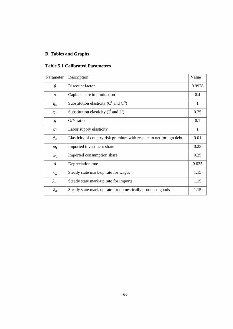
66

B. Tables and Graphs

Table 5.1 Calibrated Parameters Parameter Description Value

O Discount factor 0.9928

F Capital share in production 0.4

±v Substitution elasticity (Cd and Cm) 1

±, Substitution elasticity (Id and Im) 0.25

¸ G/Y ratio 0.1

~Í Labor supply elasticity 1

6§ Elasticity of country risk premium with respect to net foreign debt 0.01

�, Imported investment share 0.23

�v Imported consumption share 0.25

� Depreciation rate 0.035

$% Steady state mark-up rate for wages 1.15

$h Steady state mark-up rate for imports 1.15

$/ Steady state mark-up rate for domestically produced goods 1.15

67

Table 5.2 Prior and Posterior Distributions Prior Posterior

Description Parameter Type Mean Standard Deviation

Mean Confidence

Interval

Calvo wages G% Beta 0.75 0.10 0.746 0.585 0.914

Calvo domestic prices G/ Beta 0.75 0.10 0.669 0.549 0.801

Calvo import prices Gh Beta 0.75 0.10 0.738 0.649 0.812

Indexation wages c% Beta 0.5 0.10 0.501 0.337 0.669

Indexation prices c/ Beta 0.5 0.10 0.495 0.333 0.658

Investment adj cost �ΠNormal 5 1.00 4.962 3.405 6.486

Capital adj. cost ~§ Normal 0.05 0.50 1.190 0.637 1.715

Export demand elasticity

±Ì Normal 1 0.20 0.897 0.668 1.120

Habit formation b Beta 0.7 0.10 0.881 0.806 0.968

Shock persistence

Unit root tech. &Ï,8 Beta 0.8 0.10 0.549 0.456 0.648

Stationary tech. &Ï,Ð Beta 0.8 0.10 0.768 0.610 0.917

Investment &Ï,� Beta 0.8 0.10 0.904 0.846 0.965

Preference &Ñ,v Beta 0.8 0.10 0.691 0.494 0.952

Labor supply &Ñ,y Beta 0.8 0.10 0.791 0.631 0.954

Risk premium &Ò Beta 0.8 0.10 0.868 0.814 0.929

Inflation target &d� Beta 0.8 0.10 0.791 0.649 0.941

Foreign interest rate &º∗ Beta 0.8 0.10 0.928 0.883 0.973

Foreign demand &»∗ Beta 0.8 0.10 0.887 0.804 0.973

Foreign inflation &d∗ Beta 0.8 0.10 0.271 0.188 0.360

Monetary policy rule

Smoothing parameter &º Beta 0.7 0.10 0.706 0.646 0.766

Inflation response ¡d Normal 1.4 0.10 1.422 1.343 1.497

Diff. inflation response ¡½d Normal 0.12 0.05 0.144 0.070 0.221 Exchange rate response ¡p Normal 0.0 0.05 -0.046 -0.083 -0.009

Output response ¡» Normal 0.12 0.05 0.076 0.028 0.120

Diff. output response ¡½Ó Normal 0.05 0.05 0.034 0.004 0.062

68

Table 5.2 Prior and Posterior Distributions (continued) Prior Posterior

Description Parameter Type Mean Standard Deviation

Mean Confidence

Interval

Shock volatility

Unit root technology ~Ï,8 Inverse gamma

0.03 2.00 0.066 0.055 0.080

Stationary technology

~Ï,Ð Inverse gamma

0.03 2.00 0.025 0.009 0.041

Marginal efficiency of investment ~�

Inverse gamma

0.03 2.00 0.131 0.089 0.174

Preference 'Ñ,v Inverse gamma

0.03 2.00 0.362 0.158 0.545

Labor supply 'Ñ,y Inverse gamma

0.03 2.00 0.034 0.006 0.074

Risk premium 'Ò Inverse gamma

0.03 2.00 0.011 0.007 0.015

Monetary policy 'º Inverse gamma

0.03 2.00 0.006 0.005 0.007

Inflation target 'dÀ Inverse gamma

0.03 2.00 0.011 0.007 0.016

Domestic mark-up '�,/ Inverse gamma

0.05 2.00 0.065 0.012 0.148

Import mark-up '�,h Inverse gamma

0.05 2.00 0.539 0.245 0.808

Exogenous spending '�,/ Inverse gamma

0.03 2.00 0.215 0.172 0.258

Foreign demand '»∗ Inverse gamma

0.01 2.00 0.092 0.073 0.111

Foreign interest rate 'º∗ Inverse gamma

0.01 2.00 0.002 0.001 0.002

Foreign inflation 'd∗ Inverse gamma

0.01 2.00 0.065 0.054 0.077

69

Table 5.3 Posterior variance decomposition in the model

Shock/ Series Output Consumption Investment

Stationary technology 1.78 0.02 1.2

Unit root technology 62.62 34.53 47.64 Preference 4.97 63.61 3.87

Labor supply 0.03 0.00 0.03

Domestic mark-up 0.32 0.00 0.03

Import mark-up 0.03 0.01 0.44

Risk premium 4.30 0.02 1.32

Marginal efficiency of investment 10.22 1.59 43.6 Monetary policy 0.78 0.00 0.17

Foreign inflation 1.00 0.00 0.00

Foreign demand 1.66 0.19 0.94

Foreign interest rate 0.29 0.00 0.16

Exogenous spending 11.64 0.02 0.51

Inflation target 0.34 0.00 0.09

70

Figure 5.1a Prior and posterior distributions (Parameters)

71

Figure 5.1b Prior and posterior distributions (Monetary policy parameters)

Figure 5.1c Prior and posterior distributions (Shock processes parameter)

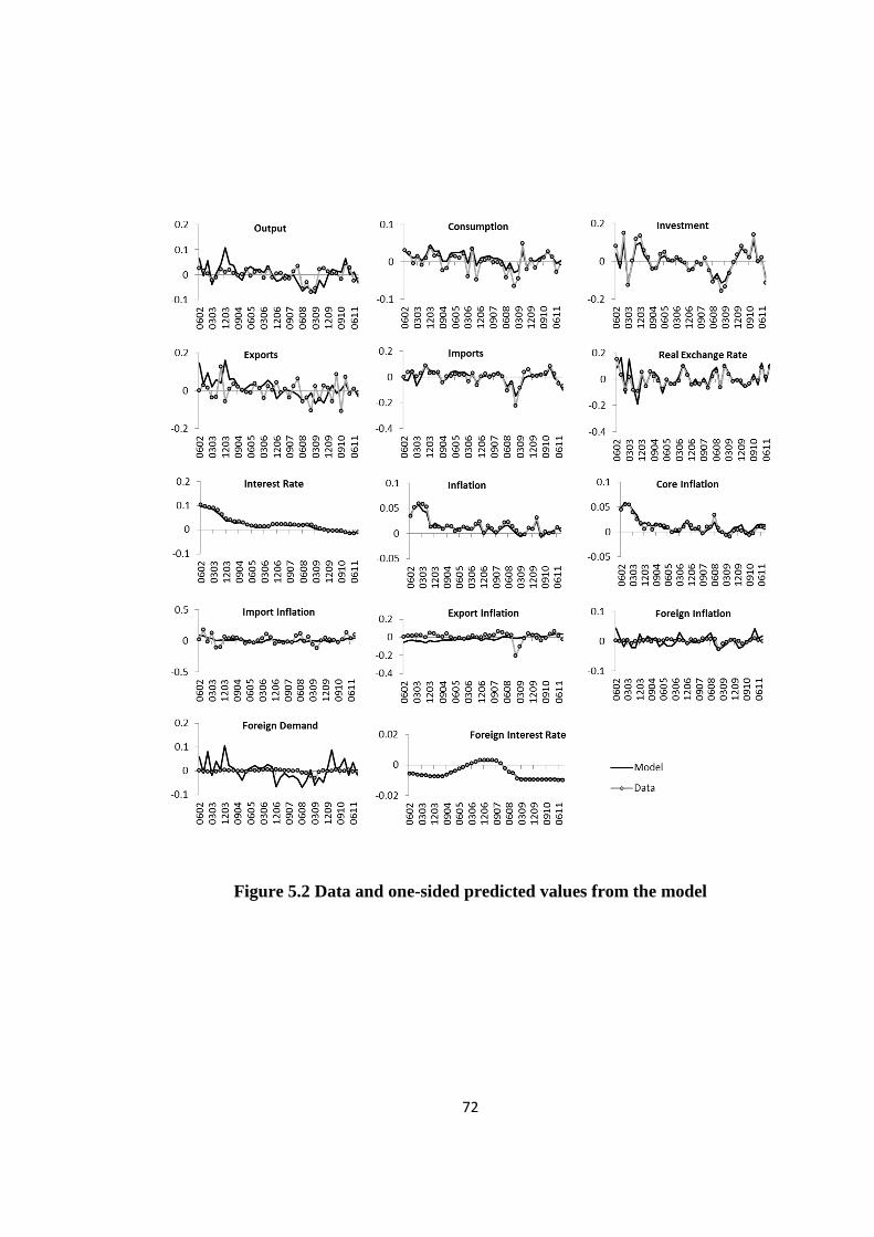
72

Figure 5.2 Data and one-sided predicted values from the model

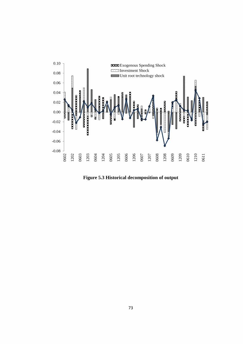
73

Figure 5.3 Historical decomposition of output

-0.08

-0.06

-0.04

-0.02

0.00

0.02

0.04

0.06

0.08

0.100

602

120

2

060

3

120

3

060

4

120

4

060

5

120

5

060

6

120

6

060

7

120

7

060

8

120

8

060

9

120

9

061

0

121

0

061

1

Exogenous Spending ShockInvestment ShockUnit root technology shock

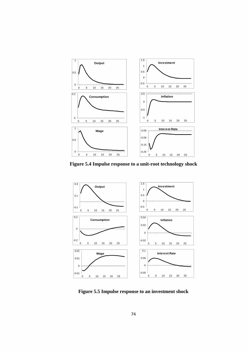
74

Figure 5.4 Impulse response to a unit-root technology shock

Figure 5.5 Impulse response to an investment shock

0

0.5

1

0 5 10 15 20 25

Output

0

0.2

0 5 10 15 20 25

Consumption

-0.5

0

0.5

1

1.5

0 5 10 15 20 25

Investment

-1

-0.5

0

0.5

0 5 10 15 20 25

Inflation

0

0.5

1

0 5 10 15 20 25

Wage

-0.25

-0.15

-0.05

0.05

0 5 10 15 20 25

Interest Rate

-0.1

0.1

0.3

0 5 10 15 20 25

Output

-0.2

0

0.2

0 5 10 15 20 25

Consumption

-0.5

0

0.5

1

1.5

0 5 10 15 20 25

Investment

-0.02

0

0.02

0.04

0 5 10 15 20 25

Inflation

-0.01

0

0.01

0.02

0 5 10 15 20 25

Wage

-0.05

0

0.05

0.1

0 5 10 15 20 25

Interest Rate

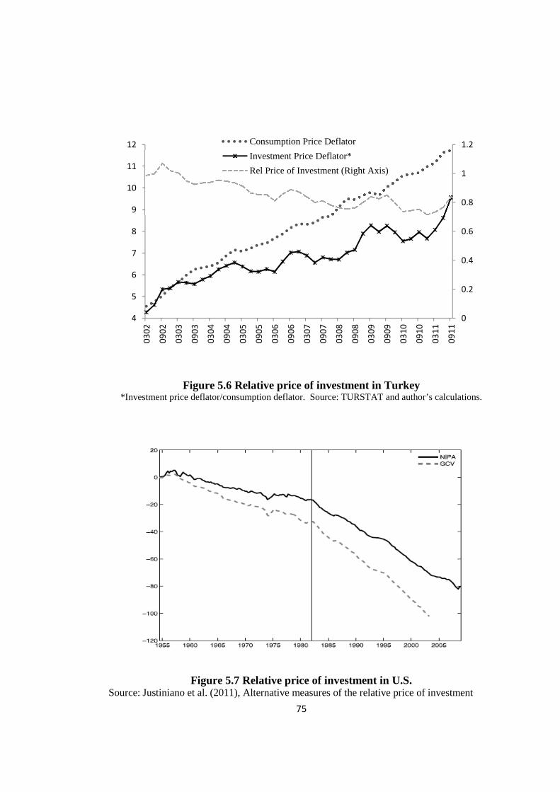
75

Figure 5.6 Relative price of investment in Turkey

*Investment price deflator/consumption deflator. Source: TURSTAT and author’s calculations.

Figure 5.7 Relative price of investment in U.S.

Source: Justiniano et al. (2011), Alternative measures of the relative price of investment

0

0.2

0.4

0.6

0.8

1

1.2

4

5

6

7

8

9

10

11

120

30

2

09

02

03

03

09

03

03

04

09

04

03

05

09

05

03

06

09

06

03

07

09

07

03

08

09

08

03

09

09

09

03

10

09

10

03

11

09

11

Consumption Price Deflator

Investment Price Deflator*

Rel Price of Investment (Right Axis)

76

TEZ FOTOKOP İSİ İZİN FORMU

ENSTİTÜ Fen Bilimleri Enstitüsü

Sosyal Bilimler Enstitüsü Uygulamalı Matematik Enstitüsü Enformatik Enstitüsü Deniz Bilimleri Enstitüsü YAZARIN Soyadı : Yüksel Adı : Canan Bölümü : İktisat TEZİN ADI (İngilizce) : Role of Investment Shocks in Explaining Business Cycles in Turkey TEZİN TÜRÜ : Yüksek Lisans Doktora 1. Tezimin tamamından kaynak gösterilmek şartıyla fotokopi alınabilir. 2. Tezimin içindekiler sayfası, özet, indeks sayfalarından ve/veya bir bölümünden kaynak gösterilmek şartıyla fotokopi alınabilir. 3. Tezimden bir (1) yıl süreyle fotokopi alınamaz. TEZİN KÜTÜPHANEYE TESL İM TAR İHİ: